High Speed Ground Penetrating Radar for Road Pavement and

Bridge Structural Inspection and Maintenance

Final Report

Project Number: SPR-RSCH017-738

Project Investigators

Tian Xia (PI), Associate Professor

School of Engineering

University of Vermont

Dryver Huston (Co-PI), Professor

School of Engineering

University of Vermont

Report Submitted on: 06/30/2016

DISCLAIMER

This research was funded by the Vermont Transportation Agency. The contents of this

report reflect the views of the authors, who are responsible for the facts and the accuracy of the

information presented herein. The contents do not necessarily reflect the official views or policies

of Vermont Transportation Agency. Neither does this report constitute a standard, specification, or

regulation. Also, mention of trade names or commercial products does not constitute endorsement

or recommendation for use.

Chapter 1. Introduction

In March 2014, ASCE (American Society of Civil Engineering) published the America’s

Infrastructure Report Card to provide a comprehensive assessment of current infrastructure

conditions and needs in U.S. The report card adopts a simple school report card format by assigning

A to F grades and making recommendations for how to raise the grades. According to the report

card, the accumulated GPA for America’s infrastructure is rated as D+, which indicates that “the

infrastructure is in poor to fair condition and mostly below standard, with many elements

approaching the end of their services life. A large portion of the system exhibits significant

deterioration. Condition and capacity are of significant concern with strong risk of failure”. The

report card also provides infrastructure grades of each state. For Vermont, its roads grade is C- and

the bridges grade is C. Vermont has 14,291 public road miles. 14% of them are in poor condition.

Among 2,731 Vermont bridges, 30% are considered structurally deficient, and 643 or 23.6% are

considered functionally obsolete. A deficient or obsolete road or bridge, when left open to traffic,

requires significant maintenance and repair to remain in service and eventual rehabilitation or

replacement, which necessitates a huge amount of capital investments. For instance, the Federal

Highway Administration (FHWA) estimates that to eliminate the nation’s bridge deficient backlog

by 2028, it would need to invest $20.5 billion annually, while only $12.8 billion is being spent

currently. For roads improvements, $170 billion in capital investment would be needed on an

annual basis, while the current level is only $91 billion. Therefore, to effectively allocate and utilize

the tight resources for road and bridge maintenance and condition improvements are vital.

To leverage roadway and bridge structural reliability and extend their usable lifetime, it is

important to closely monitor their structural conditions effectively and efficiently. Early and

accurate detection, localization and assessment of damages or defect in pavement and bridge deck

are of great values for scheduling maintenance and rehabilitation activities, and can significantly

reduce the damage progression and maintenance costs. To achieve these goals, developing and

applying appropriate tools and measurement methodologies are indispensable.

Bridge decks can suffer from various defects, such as cracks, spalling, scaling, honeycomb,

voids, delamination, insufficient cover, corrosion of rebar, etc. Corrosion of rebar is one of the

dominant damage types in terms of overall bridge maintenance costs. One major cause of rebar

corrosion is due to the use of deicing salts, where the ingress of chloride ions causes corrosion,

which causes cracking and then a positive feedback situation where the cracking enables more

chloride intrusion. This effect can be critical in Vermont since deicing salt is widely applied

throughout the long winter season.

Conventional techniques for bridge deck condition assessment, including core sampling,

corrosion (half-cell) potentials, and chloride ion measurements are slow, labor intensive, intrusive

to traffic, and do not produce an accurate estimate of the quantity of deteriorated concrete.

Corrosion potentials and chloride ion measurements infer corrosion, but do not address unseen

freeze/thaw damage. A more reliable technique, the chain drag, does not work with either asphalt

overlays or in heavy traffic conditions with high ambient noise.

For roadway asphalt pavement, the in-situ density is regarded as one of the most important

controls to ensure that a pavement being placed is of high quality because it is a good indicator of

future performance. In-situ density is frequently assessed utilizing three methods: cores, nuclear

density gauge measurements or non-nuclear density gauge measurements. However, these

methods are destructive; only provide density readings at discrete sampling locations. Moreover,

they are slow and may cause disturbance to road traffic. These drawbacks limit their applications

for pavement profile assessment during the roadway construction and lifetime maintenance.

Presently, innovative nondestructive testing (NDT) technologies are increasingly adopted

by many transportation agencies. In a recent SHRP 2 (Strategic Highway Research Program)

project, a team of industry and academia collaborators are investigating different NDT methods to

detect deterioration in concrete bridge decks in Haymarket, Virginia [1]. Among all NDT

techniques, GPR is one of the most important tools enabling subsurface structural

characterizations. In its operation, the GPR transmitter antenna radiates the electromagnetic (EM)

wave into the subsurface structure under test. The EM wave traveling velocity in the structure is

determined primarily by the permittivity or dielectric constant of the subsurface material. When

the EM wave hits features or objects that have electrical properties differing from the surrounding

medium, it will be reflected and received by the receiver antennas. The dependence of signal

traveling velocity and amplitude on the material electrical properties will result in different

reflection waveforms. By performing data analysis of the reflection signals, the subsurface

structural features can be effectively characterized.

Although the strength of GPR has been demonstrated in various case studies, there are still

many challenging factors needing further investigations. Moreover, in Vermont, since the

experience of applying GPR is very limited, many issues require intensive studies. For instance,

how to use GPR to accurately measure pavement and bridge deck structural parameters, how to

characterize the effects of harsh weather conditions and the usage of deicing salt on roadway and

bridge deck, and how to best utilize GPR test data to facilitate decision makings for maintenance,

prioritizing resource allocations, determining the scope of required repairs and rehabilitation, etc,

are not well understood. In addition, existing GPR systems still have performance limitations.

According to Uddin [2], it is reported that the scan rates of most commercial highway speed (i.e.

60 mph) GPRs are low, i.e. 50 scans/second. When GPR vehicle’s speed is 60 mph, over 0.6

meters spatial offset occurs between two adjacent scans, which produces large “blind spots”

missing for characterizations. One simple solution is to reduce the GPR vehicle speed. For

instance, by moving a handcart GPR at 1 mph, the inspection range resolution can research 1 cm,

which is compatible with most bridge deck rebar diameters. However, such a low survey speed

will cause significant interruption of normal traffic and may require shutdown of the roadway or

bridge.

1.1 Project Objectives:

The overarching objective of this research is the development of a systematic methodology

of employing GPR, including instruments, subsequent data processing and interpretation that can

be used regularly as part of a roadway pavement and bridge evaluation program. Test

methodologies and procedures that are suitable for Vermont environmental and infrastructural

conditions are explored and evaluated. Moreover, we implement and improve a high speed GPR

system that allows driving speed roadway and bridge deck inspection with leveraged inspection

resolution.

We investigate the strengths and limitations of GPR to determination the correct

implementation both in terms of operation and data assessment, and the range of road conditions

for which usage is worthwhile. The ultimate goal is to make GPR a suitable tool to facilitate

transportation infrastructure survey, maintenance, repair and rehabilitation in Vermont and

beyond. The research objectives are:

1.2 Research Methodologies:

To achieve the above objectives, the research is carried out with three major parts: 1). GPR

system hardware design and improvement; 2). GPR signal processing algorithms investigation and

development; 3). Field test for GPR performance validation and function exploration.

Chapter 2. GPR System Hardware Design and Improvement

2.1 Impulse GPR Design:

The development of new impulse ground penetrating radar is of great value for evaluating the

structural conditions of transportation infrastructure. For such particular applications, the key

factors to consider include the scanning speed and the inspection accuracy. Various factors, such

as the relatively low signal sampling rate, bulky mechanical structure, and ground coupled

antennas installed in close proximity to the detection surface, are critical in determining GPR

scanning speeds and scanning performance. Many of these limitations arise from speed processing

restrictions and the need to comply with the United States Federal Communications Commission

(FCC)’s radiated electromagnetic emission restrictions. The research in this project aims at

overcoming these drawbacks and constraints by developing a new and small air-launched UWB

GPR system that can be installed on the vehicle to operate at the normal driving speed.

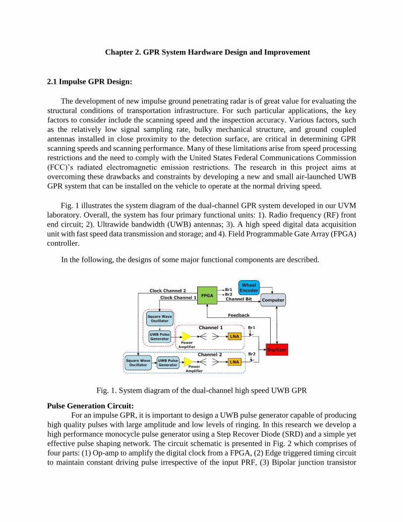
Fig. 1 illustrates the system diagram of the dual-channel GPR system developed in our UVM

laboratory. Overall, the system has four primary functional units: 1). Radio frequency (RF) front

end circuit; 2). Ultrawide bandwidth (UWB) antennas; 3). A high speed digital data acquisition

unit with fast speed data transmission and storage; and 4). Field Programmable Gate Array (FPGA)

controller.

In the following, the designs of some major functional components are described.

Fig. 1. System diagram of the dual-channel high speed UWB GPR

Pulse Generation Circuit:

For an impulse GPR, it is important to design a UWB pulse generator capable of producing

high quality pulses with large amplitude and low levels of ringing. In this research we develop a

high performance monocycle pulse generator using a Step Recover Diode (SRD) and a simple yet

effective pulse shaping network. The circuit schematic is presented in Fig. 2 which comprises of

four parts: (1) Op-amp to amplify the digital clock from a FPGA, (2) Edge triggered timing circuit

to maintain constant driving pulse irrespective of the input PRF, (3) Bipolar junction transistor

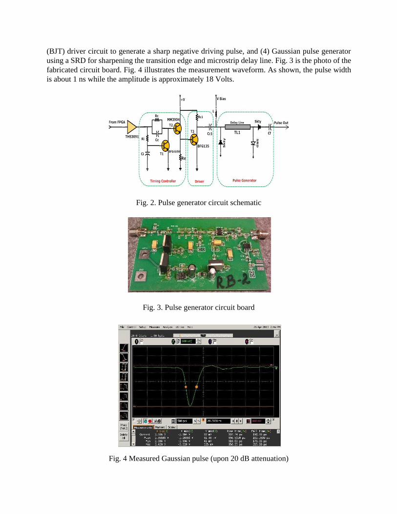
(BJT) driver circuit to generate a sharp negative driving pulse, and (4) Gaussian pulse generator

using a SRD for sharpening the transition edge and microstrip delay line. Fig. 3 is the photo of the

fabricated circuit board. Fig. 4 illustrates the measurement waveform. As shown, the pulse width

is about 1 ns while the amplitude is approximately 18 Volts.

Fig. 2. Pulse generator circuit schematic

Fig. 3. Pulse generator circuit board

Fig. 4 Measured Gaussian pulse (upon 20 dB attenuation)

UWB Antenna:

A TEM horn antenna is designed with the focus to improve impedance matching spanning

the whole ultra-wide frequency band. EM simulation and structure optimization are performed to

smooth out EM signal propagation. Experimental results show that the antennas can achieve very

low ringing effects and good signal fidelity.

For impulse GPR antenna design, one critical challenge is to achieve impedance matching

across ultra-wide frequency band. There are two main structural points needing intensive

considerations, one is the feed port, and the other is the interface at the antenna aperture. For the

air coupled GPR antenna, the characteristic impedance at aperture is 377 Ohm, while the feed line

impedance is 50 Ohms. Design measures need to resolve this mismatch by gradually

accomplishing impedance transition to minimize reflections.

Fig.5 illustrates our developed UWB antenna. As shown, the antenna structure consists of

three sections: feed line, waveguide taper segment and a rounded shaped aperture. The feed line

and the taper section can be modeled as a series of N parallel-plate transmission line segments.

Each segment consists of two metal plates that are separated by a dielectric media with varying

width.

In order to characterize the parallel plate structure, an analytical model is developed to

study the effect of feed point length L0 on feed line input impedance across wide frequency band.

The model assumes 50 ohms output impedance, which is replaced by the actual input impedance

of the taper section later in the full model. The feed line width is W0, feed line height is d0.

Simulations show that when L0 = 6mm, d0 = 3mm and W0 = 12mm, the feed line demonstrates

minimal impedance variations across the frequency band ranging from 600 MHz to 6 GHz.

Fig. 5– Top view and side view of the horn antenna

Fig. 5– Top view and side view of the horn antenna

To further improve antenna performance, extra structure optimization measures are taken.

One structure change is rounding the edges at the feed point. Fig. 6a and Fig. 6b illustrate the

traditional sharp edges versus the edge rounding at feed point respectively. Results in Fig. 6c

demonstrates that the rounded corners structure leads to the improved S11 performance. The

second structure optimization measure is rounding the flare edges. Fig. 7a and Fig. 7b illustrate

two flare edges. Fig. 7c is the simulation resulting validating the performance improvement.

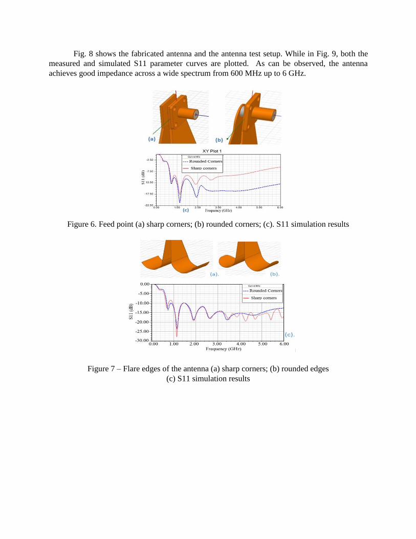
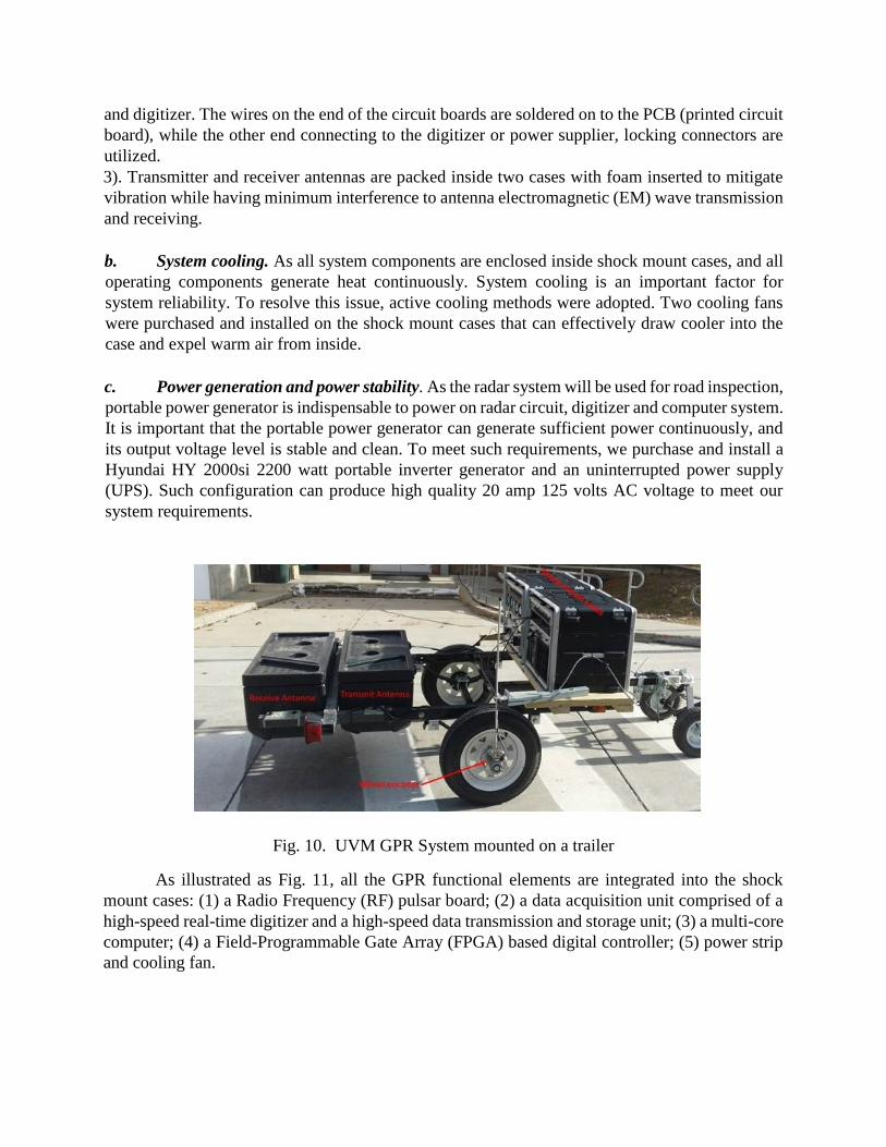
Fig. 8 shows the fabricated antenna and the antenna test setup. While in Fig. 9, both the

measured and simulated S11 parameter curves are plotted. As can be observed, the antenna

achieves good impedance across a wide spectrum from 600 MHz up to 6 GHz.

Figure 6. Feed point (a) sharp corners; (b) rounded corners; (c). S11 simulation results

Figure 7 – Flare edges of the antenna (a) sharp corners; (b) rounded edges

(c) S11 simulation results

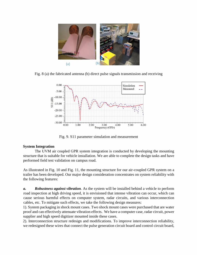
Fig. 8 (a) the fabricated antenna (b) direct pulse signals transmission and receiving

Fig. 9. S11 parameter simulation and measurement

System Integration

The UVM air coupled GPR system integration is conducted by developing the mounting

structure that is suitable for vehicle installation. We are able to complete the design tasks and have

performed field test validation on campus road.

As illustrated in Fig. 10 and Fig. 11, the mounting structure for our air-coupled GPR system on a

trailer has been developed. Our major design consideration concentrates on system reliability with

the following features:

a. Robustness against vibration. As the system will be installed behind a vehicle to perform

road inspection at high driving speed, it is envisioned that intense vibration can occur, which can

cause serious harmful effects on computer system, radar circuits, and various interconnection

cables, etc. To mitigate such effects, we take the following design measures:

1). System packaging in shock mount cases. Two shock mount cases were purchased that are water

proof and can effectively attenuate vibration effects. We have a computer case, radar circuit, power

supplier and high speed digitizer mounted inside these cases.

2). Interconnection structure redesign and modifications. To improve interconnection reliability,

we redesigned these wires that connect the pulse generation circuit board and control circuit board,

and digitizer. The wires on the end of the circuit boards are soldered on to the PCB (printed circuit

board), while the other end connecting to the digitizer or power supplier, locking connectors are

utilized.

3). Transmitter and receiver antennas are packed inside two cases with foam inserted to mitigate

vibration while having minimum interference to antenna electromagnetic (EM) wave transmission

and receiving.

b. System cooling. As all system components are enclosed inside shock mount cases, and all

operating components generate heat continuously. System cooling is an important factor for

system reliability. To resolve this issue, active cooling methods were adopted. Two cooling fans

were purchased and installed on the shock mount cases that can effectively draw cooler into the

case and expel warm air from inside.

c. Power generation and power stability. As the radar system will be used for road inspection,

portable power generator is indispensable to power on radar circuit, digitizer and computer system.

It is important that the portable power generator can generate sufficient power continuously, and

its output voltage level is stable and clean. To meet such requirements, we purchase and install a

Hyundai HY 2000si 2200 watt portable inverter generator and an uninterrupted power supply

(UPS). Such configuration can produce high quality 20 amp 125 volts AC voltage to meet our

system requirements.

Fig. 10. UVM GPR System mounted on a trailer

As illustrated as Fig. 11, all the GPR functional elements are integrated into the shock

mount cases: (1) a Radio Frequency (RF) pulsar board; (2) a data acquisition unit comprised of a

high-speed real-time digitizer and a high-speed data transmission and storage unit; (3) a multi-core

computer; (4) a Field-Programmable Gate Array (FPGA) based digital controller; (5) power strip

and cooling fan.

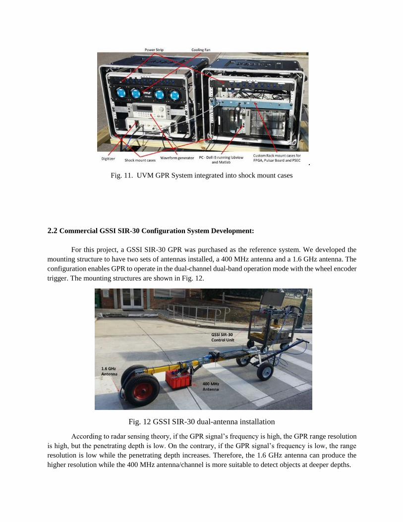
Fig. 11. UVM GPR System integrated into shock mount cases

2.2 Commercial GSSI SIR-30 Configuration System Development:

For this project, a GSSI SIR-30 GPR was purchased as the reference system. We developed the

mounting structure to have two sets of antennas installed, a 400 MHz antenna and a 1.6 GHz antenna. The

configuration enables GPR to operate in the dual-channel dual-band operation mode with the wheel encoder

trigger. The mounting structures are shown in Fig. 12.

Fig. 12 GSSI SIR-30 dual-antenna installation

According to radar sensing theory, if the GPR signal’s frequency is high, the GPR range resolution

is high, but the penetrating depth is low. On the contrary, if the GPR signal’s frequency is low, the range

resolution is low while the penetrating depth increases. Therefore, the 1.6 GHz antenna can produce the

higher resolution while the 400 MHz antenna/channel is more suitable to detect objects at deeper depths.

Chapter 3. GPR Signal Processing

In the project, great efforts were invested investigating and exploring GPR signal

processing algorithms to leverage GPR sensing performance. In the following sections, these

algorithms are described.

3.1 Asphalt Pavement Thickness Estimation Method:

Asphalt pavement thickness measurement is important for pavement quality evaluation.

Traditional destructive measurement methods are slow, expensive and inefficient. In this project,

a GPR based non-destructive measurement method was developed. Specifically, a 3-step signal

processing method was implemented as described below:

Step 1: Stack every 5 GPR A-Scan traces to calculate average value to increase the signal to noise

ratio.

Step 2: Remove the DC offset in A-Scan trace.

Step 3: Top and bottom surface of asphalt pavement identification using Hilbert Transform.

In our GPR system, the Hilbert Transform was implemented to extract the pulse envelope that

measures the signal power. The Hilbert Transform of signal 𝑠(𝑡) can be considered as the

convolution of 𝑠(𝑡) with the function , which can be expressed as

(1)

To eliminate the singularities, such as 𝜏 = 𝑡 and 𝜏 = ±∞, the Hilbert Transform is defined using

the Cauchy principal value. Correspondingly, the Hilbert Transform of 𝑠(𝑡) is given by

(2)

Applying the Hilbert transform to GPR signal 𝑠(𝑡), the analytic signal is obtained as

𝑠𝑎(𝑡) = 𝑠(𝑡) + 𝑖𝑠 (𝑡) (3)

where 𝑠 (𝑡) is the direct output of the Hilbert Transform of 𝑠(𝑡). The magnitude of 𝑠𝑎(𝑡) equals

|𝑠𝑎(𝑡)| = √𝑠(𝑡)2 + 𝑠 (𝑡)2 (4)

|𝑠𝑎(𝑡)| is the envelope of 𝑠(𝑡), which facilitates the signal power characterization.

Fig. 13 demonstrates signal power characterization using the Hilbert transform. The signal in Fig.

13(a) is a GPR A-Scan waveform produced from two scatters. In the A-Scan waveform, the first

pulse is the antennas’ direct coupling, while the second and third pulses are the reflection signal

from the 1st and 2nd scatters correspondingly. The transmitting pulse signal is the Ricker wavelet

(the second order derivatives of Gaussian function), the backscattering pulse from each object or

layer interface shows three peaks. Fig. 13(b) shows the waveform produced by the Hilbert

transform where the three peaks become much more discernible.

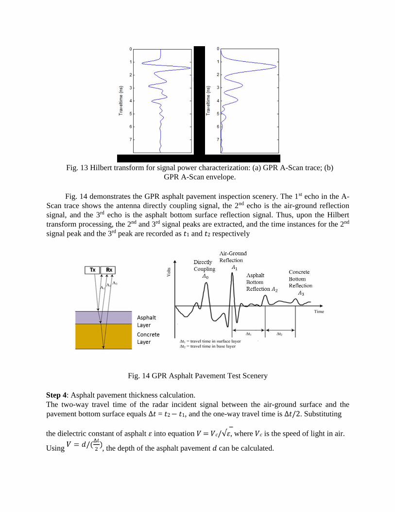
Fig. 13 Hilbert transform for signal power characterization: (a) GPR A-Scan trace; (b)

GPR A-Scan envelope.

Fig. 14 demonstrates the GPR asphalt pavement inspection scenery. The 1st echo in the A-

Scan trace shows the antenna directly coupling signal, the 2nd echo is the air-ground reflection

signal, and the 3rd echo is the asphalt bottom surface reflection signal. Thus, upon the Hilbert

transform processing, the 2nd and 3rd signal peaks are extracted, and the time instances for the 2nd

signal peak and the 3rd peak are recorded as 𝑡1 and 𝑡2 respectively

Fig. 14 GPR Asphalt Pavement Test Scenery

Step 4: Asphalt pavement thickness calculation.

The two-way travel time of the radar incident signal between the air-ground surface and the

pavement bottom surface equals Δ𝑡 = 𝑡2 − 𝑡1, and the one-way travel time is Δ𝑡/2. Substituting

the dielectric constant of asphalt 𝜀 into equation 𝑉 = 𝑉𝑐/√𝜀, where 𝑉𝑐 is the speed of light in air.

Using , the depth of the asphalt pavement 𝑑 can be calculated.

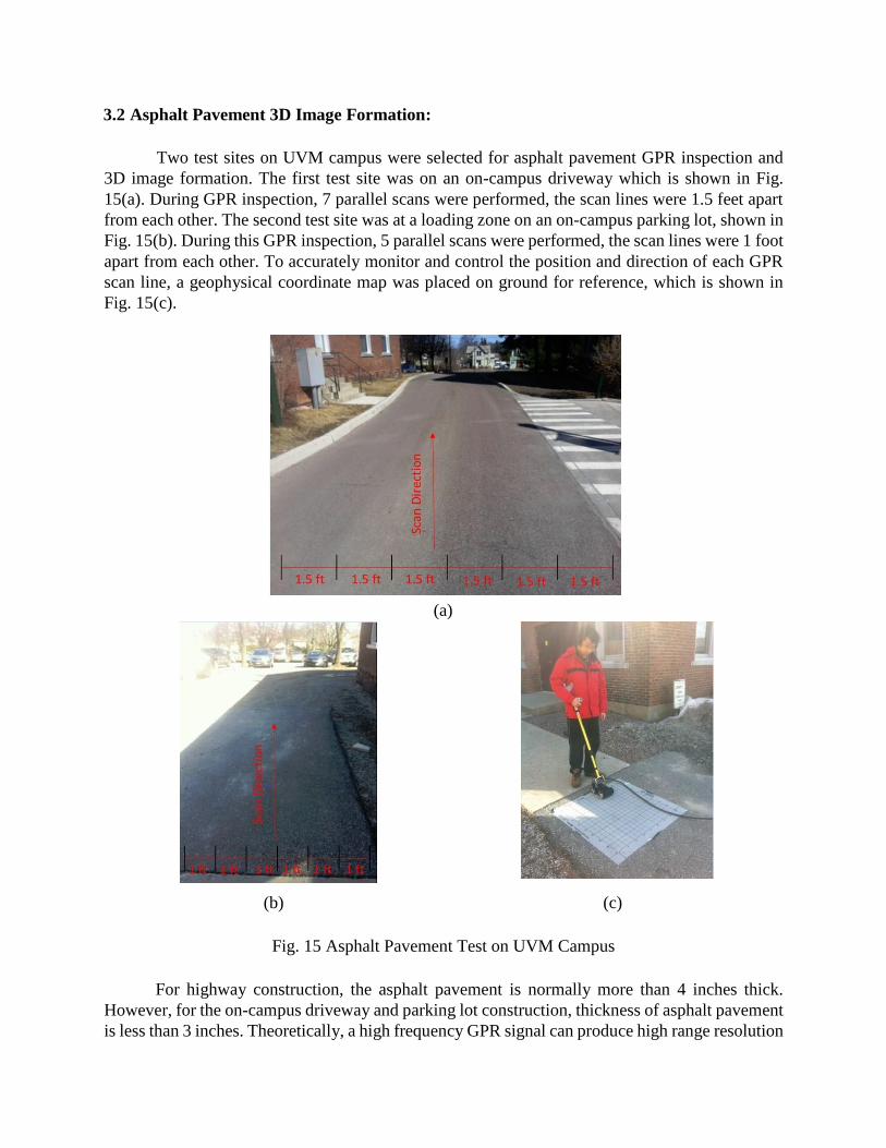
3.2 Asphalt Pavement 3D Image Formation:

Two test sites on UVM campus were selected for asphalt pavement GPR inspection and

3D image formation. The first test site was on an on-campus driveway which is shown in Fig.

15(a). During GPR inspection, 7 parallel scans were performed, the scan lines were 1.5 feet apart

from each other. The second test site was at a loading zone on an on-campus parking lot, shown in

Fig. 15(b). During this GPR inspection, 5 parallel scans were performed, the scan lines were 1 foot

apart from each other. To accurately monitor and control the position and direction of each GPR

scan line, a geophysical coordinate map was placed on ground for reference, which is shown in

Fig. 15(c).

(a)

(b) (c)

Fig. 15 Asphalt Pavement Test on UVM Campus

For highway construction, the asphalt pavement is normally more than 4 inches thick.

However, for the on-campus driveway and parking lot construction, thickness of asphalt pavement

is less than 3 inches. Theoretically, a high frequency GPR signal can produce high range resolution

while having a low penetrating depth, while a low frequency GPR signal has deeper penetrating

depth but at the cost of a lower range resolution. In this experiment, in order to achieve a high

range resolution for thin asphalt layer measurement, the high frequency 2.3 GHz Mala CX GPR

system in our lab was utilized as the test device.

Fig. 16 plots the B-Scan image for one scan line at the first test site. In the image, the air-

ground interface and asphalt pavement bottom surface are marked respectively. The thickness of

the asphalt pavement on this scan line is relatively even and smooth. Combining all 7 scan lines,

the thickness map for the first test site is plotted in Fig. 17. The horizontal axis in this figure

specifies GPR travel distance in the scan direction, while the vertical axis specifies the width of

the scanning area. The color-to-thickness mapping is shown on the right. From the thickness map,

it is observed that at the center portion of this on-campus driveway, the asphalt pavement thickness

is smaller than that the border portion. We think it is because this driveway has a single lane, most

traffic loads utilize the center portion of the road, which causes the center portion of the pavement

to be thinner.

Fig. 16 B-Scan Image for One Scan Line on the 1st Test Site

Fig. 17 Asphalt Pavement Thickness Map for the 1st Test Site

Fig.18 plots the B-Scan image for the 2nd GPR scan line on the second test site. The air-

ground interface and asphalt pavement bottom surface are marked in the B-Scan image

respectively. The thickness of the asphalt pavement on this scan line decreases from the starting

point to the ending point. Combining all 5 scan lines, the thickness map is plotted in Fig. 19.

Fig. 18 B-Scan Image for One Scan Line on the 2nd Test Site

Fig. 19 Asphalt Pavement Thickness Map for the 2nd Test Site

3.3 Asphalt Pavement Dielectric Constant Monitoring:

The winter in Vermont is quite long and cold, so the snow and ice accumulates on the

asphalt pavement during the winter. Also, water sinks under the asphalt pavement after raining.

When pavement moisture changes, the dielectric constant of the asphalt pavement will be different.

In this study, we explore GPR’s capability to measure the dielectric constant of the asphalt

pavement which can be utilized to assess asphalt moisture condition and proper road water

drainage.

In the experiment, three spots on a 2nd on-campus test sites were marked and selected for

measurement, which are depicted in Fig. 20. The 1st test spot was located at the border of the road

pavement. The 2nd test spot was located at the center portion of the road. This spot has a pit where

water was accumulated. The 3rd test spot was also located at the center portion of the asphalt

pavement. Two weeks of successive GPR tests on these 3 spots are performed. The dielectric

constant for these 3 spots were calculated and recorded after each test. Note, the dielectric constant

of water is much higher than the pavement, therefore a higher dielectric constant indicates a higher

degree moisture.

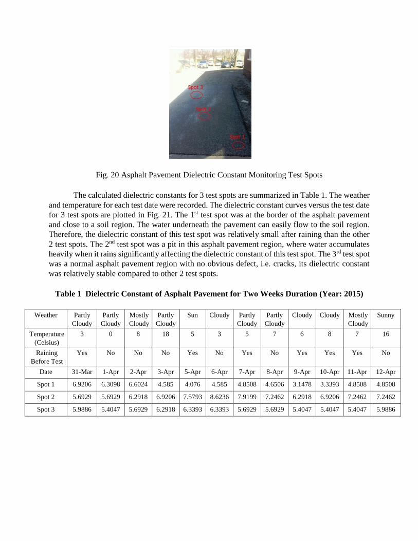
Fig. 20 Asphalt Pavement Dielectric Constant Monitoring Test Spots

The calculated dielectric constants for 3 test spots are summarized in Table 1. The weather

and temperature for each test date were recorded. The dielectric constant curves versus the test date

for 3 test spots are plotted in Fig. 21. The 1st test spot was at the border of the asphalt pavement

and close to a soil region. The water underneath the pavement can easily flow to the soil region.

Therefore, the dielectric constant of this test spot was relatively small after raining than the other

2 test spots. The 2nd test spot was a pit in this asphalt pavement region, where water accumulates

heavily when it rains significantly affecting the dielectric constant of this test spot. The 3rd test spot

was a normal asphalt pavement region with no obvious defect, i.e. cracks, its dielectric constant

was relatively stable compared to other 2 test spots.

Table 1 Dielectric Constant of Asphalt Pavement for Two Weeks Duration (Year: 2015)

Weather Partly Cloudy

Partly Cloudy

Mostly

Cloudy Partly

Cloudy Sun Cloudy Partly

Cloudy Partly

Cloudy Cloudy Cloudy Mostly

Cloudy Sunny

Temperature

(Celsius) 3 0 8 18 5 3 5 7 6 8 7 16

Raining

Before Test Yes No No No Yes No Yes No Yes Yes Yes No

Date 31-Mar 1-Apr 2-Apr 3-Apr 5-Apr 6-Apr 7-Apr 8-Apr 9-Apr 10-Apr 11-Apr 12-Apr

Spot 1 6.9206 6.3098 6.6024 4.585 4.076 4.585 4.8508 4.6506 3.1478 3.3393 4.8508 4.8508

Spot 2 5.6929 5.6929 6.2918 6.9206 7.5793 8.6236 7.9199 7.2462 6.2918 6.9206 7.2462 7.2462

Spot 3 5.9886 5.4047 5.6929 6.2918 6.3393 6.3393 5.6929 5.6929 5.4047 5.4047 5.4047 5.9886

Fig. 21 Dielectric Constant of 3 Test Spots

3.4 Design of Compressive OFDM GPR:

In this project quarter, compressive sensing (CS) coupled with OFDM technique was

investigated to develop a low-cost and high-efficiency GPR system. In this system, OFDM spread

spectrum technique was adopted for multi-tone signal radiation and receiving to leverage sensing

efficiency. By making different frequency tones orthogonal among each other, the inter-tone cross

interferences were minimized, which ensure the signal integrity. When sensing, multiple frequency

tones were employed to synthesize the narrow width pulse signal of an extremely low duty cycle.

In other words, the synthesized pulse signal was sparse in the time domain. Therefore, compressive

sensing technology was applicable to reduce the required number of frequency tones for pulse

signal synthesis while not compromising the sensing accuracy.

The compressive OFDM GPR operates in the frequency domain, where a reduced set of

frequency tones are emitted concurrently. By collecting the corresponding frequency responses

from the scatter and performing CS reconstruction, the full spectrum response can be recovered.

Using inverse Fourier transform, the scatter’s time domain response signals are then computed,

which allows for the formulation and characterization of the GPR image.

According to the principle of CS, the signal reconstruction accuracy for compressive

OFDM GPR is highly dependent on the sparsity of the synthesized object signal in the time domain.

If the object signal is highly sparse, less frequency tones are needed for reconstruction. However,

the signal sparsity in compressive sensing OFDM GPR suffers from the impact of clutter. Clutter

is the unwanted echoes in the radar system, which are typically generated by transmitter and

receiver antennas’ direct coupling and ground surface reflection. It is relatively easy to remove

antennas direct coupling due to the time separation between the direct coupling signal and other

backscattering. While for the ground surface reflection, it is difficult to be removed as it typically

overlaps with the backscattering signals from the shallowly buried objects. The presence of strong

ground reflection decreases the sparsity of the response signal synthesized in the time domain,

0

2

4

6

8

10

Test Date

Spot 1 Spot 2 Spot 3

which can dramatically degrade CS signal recovery accuracy. As the compressive OFDM GPR

performs sensing directly in frequency mode, a frequency domain clutter removal technique to

suppress ground surface reflection signal before CS reconstruction is highly desirable. A clutter

removal (CR) technique was also developed that can directly remove the interfering ground surface

reflection in the frequency domain so that high sensing accuracy and compression ratio can be

accomplished.

Fig. 22 depicts the operating mechanism of the compressive sensing OFDM GPR. In the

operation, a set of randomly selected frequency tones were radiated concurrently using an OFDM

modulation scheme, and the echoes from the object were received. By analyzing the transmission

and receiving OFDM signals, the compressed frequency responses of the scatters, including the

gain and phase variations, were calculated. A frequency domain clutter removal was applied on

the compressed frequency response spectrum. The CS reconstruction was then performed on the

compressed frequency response data matrix to recover and synthesize the time domain response of

the full spectrum. Finally, a synthetic aperture radar (SAR) focusing algorithm was employed to

mitigate the hyperbolic distortion in the GPR B-Scan image.

Fig. 22. Compressive OFDM GPR system

For design validation, an experimental study was performed using the GPR field data

collected from scanning a 1.8 meters long on-campus concrete walkway where six reinforcing bars

are buried.

In the experiment, the OFDM signal bandwidth was set to 2 GHz to synthesize a 500 ps

wide pulse. For uncompressed OFDM GPR signal generation, 2048 frequency tones were

generated and radiated. While for the compressive OFDM implementation, 2,048 ∗ 𝑝 (0 < 𝑝 < 1)

frequency tones were randomly selected.

In the A-Scan test, the transceiver antennas were placed right above a buried rebar and 20%

of the 2048 frequency tones were randomly selected to sense and synthesize the response pulse

OFDM Transmitting

Signal

Tx Rx

OFDM Receiving

Signal

Channel

Compressive Tones

Compressive Tones

Frequency Response

Calculation

CR on Compressive

Frequency Measurements

CS Reconstruction

SAR Focusing B - Scan Image

signal. The compressed OFDM spectrum is plotted in Fig. 23(a). The compressed OFDM spectrum

after performing clutter removal processing is depicted in Fig. 23(b), and the corresponding

reconstructed A-Scan waveform is displayed in Fig. 23 (c), where the reflection signal component

corresponding to rebar reflection is pronounced.

(a) (b) (c)

Fig. 23 Reconstructed A-Scan with p=20%: (a) Compressed frequency spectrum; (b)

Compressed frequency spectrum after clutter removal; (c) Recovered A-Scan trace

Selected B-Scan images are displayed in Fig. 24. In the experiment setup, six rebars buried

in the concrete walkway were expected to be detected. When 𝑝 is higher than 30%, the

reconstructed B-Scan image was obtained with a good fidelity. When 𝑝 is reduced to 5%, the

reconstructed image becomes fuzzy, however, the signature patterns corresponding to six rebars

are still recognizable.

(a) (b)

(c) (d)

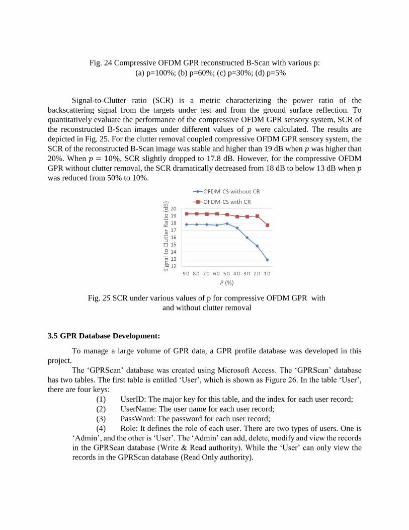
Fig. 24 Compressive OFDM GPR reconstructed B-Scan with various p:

(a) p=100%; (b) p=60%; (c) p=30%; (d) p=5%

Signal-to-Clutter ratio (SCR) is a metric characterizing the power ratio of the

backscattering signal from the targets under test and from the ground surface reflection. To

quantitatively evaluate the performance of the compressive OFDM GPR sensory system, SCR of

the reconstructed B-Scan images under different values of 𝑝 were calculated. The results are

depicted in Fig. 25. For the clutter removal coupled compressive OFDM GPR sensory system, the

SCR of the reconstructed B-Scan image was stable and higher than 19 dB when 𝑝 was higher than

20%. When 𝑝 = 10%, SCR slightly dropped to 17.8 dB. However, for the compressive OFDM

GPR without clutter removal, the SCR dramatically decreased from 18 dB to below 13 dB when 𝑝

was reduced from 50% to 10%.

Fig. 25 SCR under various values of p for compressive OFDM GPR with

and without clutter removal

3.5 GPR Database Development:

To manage a large volume of GPR data, a GPR profile database was developed in this

project.

The ‘GPRScan’ database was created using Microsoft Access. The ‘GPRScan’ database

has two tables. The first table is entitled ‘User’, which is shown as Figure 26. In the table ‘User’,

there are four keys:

(1) UserID: The major key for this table, and the index for each user record;

(2) UserName: The user name for each user record;

(3) PassWord: The password for each user record;

(4) Role: It defines the role of each user. There are two types of users. One is

‘Admin’, and the other is ‘User’. The ‘Admin’ can add, delete, modify and view the records

in the GPRScan database (Write & Read authority). While the ‘User’ can only view the

records in the GPRScan database (Read Only authority).

Figure 26 Table 'User' in the GPRScan Database

The second table is entitled ‘B-Scan’ which is shown as Figure 27. In the table ‘B-Scan’,

there are currently five keys (More keys can be added if needed):

(1) ScanID: The major key of this table, and the index for each B-Scan record;

(2) ScanTitle: The filename for this B-Scan image record;

(3) GPS: The GPS coordinate for each B-Scan image record (currently

unavailable for lab and on-campus GPR tests);

(4) Date: The date when this B-Scan data was collected;

(5) Image: The B-Scan image for each record. Figure 28 shows the B-Scan

image stored for the 2nd record whose ‘ScanTitle’ is Sidewalk Ch2.

Figure 27 Table 'B-Scan' in the GPRScan Database

Database connection and operation was implemented by MATLAB Database Toolbox.

MATLAB can use the SQL to communicate with the database. An initial database user interface

was developed using MATLAB. Based on project requirements, more sophisticated and specific

user interfaces can be developed and implemented. Figure 29 shows the current user interface that

connects to the GPRScan database via the MATLAB Database Toolbox. After connecting to the

database, users can access the GPR B-Scan data in the ‘B-Scan’ table, which is shown in Figure

30a.

To enable GPR engineers to add new database operation functions in the GPRScan

database, a MATLAB code frame was built as shown in Figure 30b. GPR engineers can insert new

SQL code into this frame to enable further data display operations, as well as insert new signal

processing code into to enable further GPR data interpretation operations.

Figure 28 B-Scan Image Stored in Each Record

Figure 29 Connect to GPRScan Database via the MATLAB Database Toolbox

Figure 30 a). Table 'B-Scan' Accessed in MATLAB; b). MATLAB Sample Code Frame

Chapter 4. GPR Field Test Applications

During the project duration, a series of field tests were conducted to verify GPR functions, explore

GPR potentials and capabilities under real world application scenarios.

4.1 GPR Field Road Test at St. Paul Street:

In September 2015, a GPR road test was conducted at St. Paul Street, downtown Burlington

where there was a road construction project between Pearl St. and Cherry St. With the assistance

of Peterson Consulting, Inc., we accessed the construction site and conducted GPR field

inspections on both the concrete sidewalk and asphalt pavement road.

The physical GPR test site picture is shown in Figure 31, and the whole test route displayed

on Google Map is shown in Figure 32. During the GPR test, a parallel bi-directional (south-to-

north and north-to-south) inspections were performed. The GPR scan direction is illustrated in

Figure 33.

Figure 31 Test Site at St. Paul Street

Figure 32 Map of the Test Site at St. Paul Street

Figure 33 Road Scan Directions

Data Processing Approaches:

The following signal processing steps were performed to enhance the GPR B-Scan images

for all the data demonstrated in this report:

Step 1: Zero-offset;

Step 2: Stack every 5 A-scan traces to calculate the average so as to increase the signal-to-

noise ratio (SNR);

Step 3: Band pass filter to remove low frequency and high frequency noise; Step

4: Signal loss compensation by amplitude rescaling along the depth axis; Step 5:

Clutter removal to remove the background signal.

Test Results Demonstration:

The processed GPR results from the parallel inspection scans were combined and plotted

in one B-Scan image. Detected objects and regions of interest are marked by the white outlined

rectangles in the B-Scan image. In the image, the horizontal axis specifies the distance from the

starting location of the scan, while the vertical axis shows the depth of the object. Figure 34 shows

the processed B-Scan image corresponding to a segment with a horizontal range between 0 and 65

feet. A pipe shown as a hyperbola in the figure was detected at a depth of 12 inch. Another region

of interest was buried at a depth of 60 inches.

Figure 34 Processed B-Scan image: 0-65 feet horizontal range

Figure 35 shows the processed B-Scan image corresponding to the segment with a

horizontal range between 65 and 125 feet. A pipe at the 78th ft mark and at a depth of 12 inches is

shown as a hyperbola in the figure below. Another pipe at the 116th ft mark and at a depth of 40

inches was also detected. Those two pipes are marked by white outlined rectangles. Two layers

were also detected and marked by white lines.

Figure 35 Processed B-Scan image: 65 -125 feet horizontal range

Figure 36 illustrates the processed B-Scan image of the segment with a horizontal range

between 125 and 185 feet. Five pipes were detected and marked by the white outlined rectangles.

One layer was detected from 133 ft to 165 ft at a 60 inch depth.

Figure 36 Processed B-Scan image: 125-185 feet horizontal range

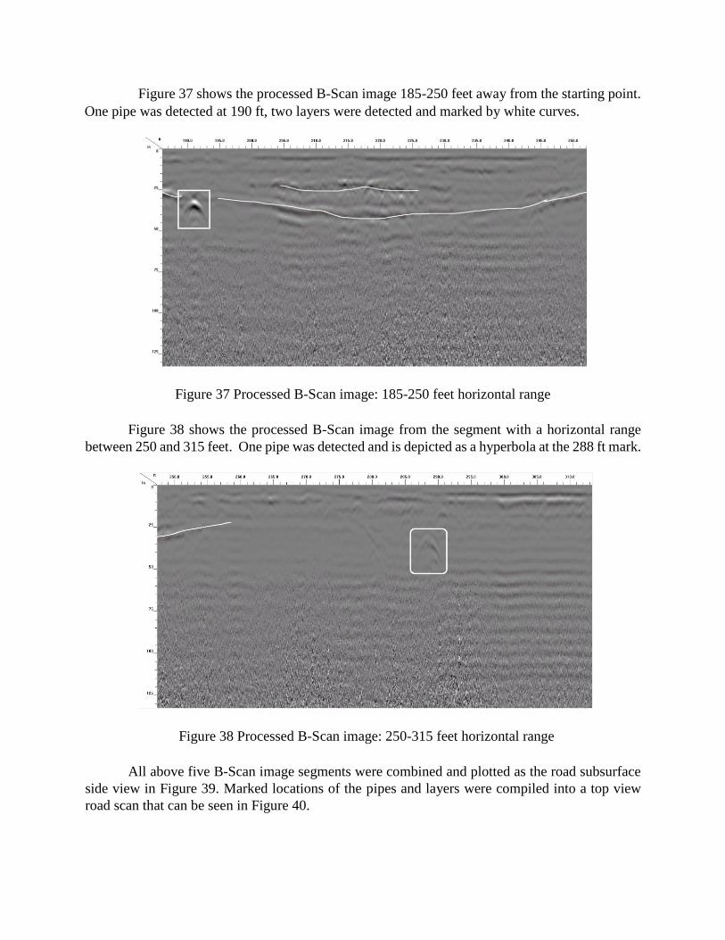
Figure 37 shows the processed B-Scan image 185-250 feet away from the starting point.

One pipe was detected at 190 ft, two layers were detected and marked by white curves.

Figure 37 Processed B-Scan image: 185-250 feet horizontal range

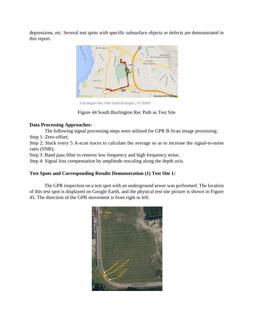
Figure 38 shows the processed B-Scan image from the segment with a horizontal range

between 250 and 315 feet. One pipe was detected and is depicted as a hyperbola at the 288 ft mark.

Figure 38 Processed B-Scan image: 250-315 feet horizontal range

All above five B-Scan image segments were combined and plotted as the road subsurface

side view in Figure 39. Marked locations of the pipes and layers were compiled into a top view

road scan that can be seen in Figure 40.

Figure 39 GPR road scan result - side view

Figure 40 GPR road scan result - top view

Ground Truths Verification:

On Oct 8, 2015, we visited the road project site at St. Paul St. to collect some ground truths

for our GPR test verification. As shown in Figure 41, a 100-foot long road section from the south

end of the test site had been excavated.

Figure 41 Road project site under excavation work

Checking the excavation site, a layer buried about 60 inches deep was detected, marked in

Figure 42. This layer’s burying depth and horizontal location agree well with our GPR inspection

results that are shown in Figure 35.

Figure 42 A layer is observed which is consistent with the GPR result in Figure 35

A metal pipe, as shown in Figure 43, was also excavated from a depth of about 12 inches.

The diameter of this metal pipe was 3 inches. This excavation result agrees with our GPR test result

shown in Figure 34.

Figure 43 An excavated pipe which was consistent with the GPR result in Figure 34

During our inspection, the road construction was on going and only part of the ground

truths were obtainable. By checking the exposed 100-foot underground structure, the GRP

inspection accuracy is well verified.

4.2 GPR Bicycle Trail Inspection:

In this test, the bicycle trail on the South Burlington Recreation Path was chosen as another

test site for GPR inspection. The test route displayed on Google Map is shown in Figure 44. The

400 MHz antenna set aims at detecting the deeper (> 3ft) objects, such as drainage pipes, sewers,

etc. The 1.6 GHz antenna set and 2.3 GHz antenna set aims at detecting small subsurface features

at shallow depth, such as pavement cracks, pavement bottom surfaces, asphalt patches and

depressions, etc. Several test spots with specific subsurface objects or defects are demonstrated in

this report.

Figure 44 South Burlington Rec Path as Test Site

Data Processing Approaches:

The following signal processing steps were utilized for GPR B-Scan image processing:

Step 1: Zero-offset;

Step 2: Stack every 5 A-scan traces to calculate the average so as to increase the signal-to-noise

ratio (SNR);

Step 3: Band pass filter to remove low frequency and high frequency noise;

Step 4: Signal loss compensation by amplitude rescaling along the depth axis.

Test Spots and Corresponding Results Demonstration (1) Test Site 1:

The GPR inspection on a test spot with an underground sewer was performed. The location

of this test spot is displayed on Google Earth, and the physical test site picture is shown in Figure

45. The direction of the GPR movement is from right to left.

Figure 45 The photo of the test site with underground sewer

The B-Scan images obtained with the 400 MHz and 1.6 GHz antenna sets are displayed in

Figure 46. The 400 MHz B-Scan image shows the underground object at a deep depth (> 3 feet or

36 inches). In the B-Scan image, a cylinder object shows hyperbolic signature. The hyperbola

representing the sewer can be observed at a 70 inch depth in the 400 MHz B-Scan image. Also,

the subsurface concrete-soil interface was observed at a 37 inch depth.

Figure 46 B-Scan Image of Sewer from 400 MHz (Top) and 1.6 GHz (Bottom) Antenna Sets

Figure 47 displays a B-Scan image obtained using the 2.3 GHz antenna set. The B-Scan

image derived from a high frequency antenna set shows small objects or features at a shallow depth

(< 3 feet or 36 inches). In this B-Scan image, the curve representing the asphalt pavement’s bottom

surface was detected.

Figure 47 B-Scan Image of Sewer from 2.3 GHz Antenna Set

(2) Test Site 2:

A GPR inspection on a test spot with a medium size asphalt patch on the surface was

performed. The physical test site picture is shown in Figure 48. The medium size asphalt patch is

marked with a yellow circle.

Figure 48 Test Spot with Medium Asphalt Patch and Small Asphalt Depression

The B-Scan images from the 400 MHz and 1.6 GHz antenna sets are displayed in Figure

49. In 400 MHz B-Scan image (the top image), the subsurface concrete-soil interface was detected

at a 26 inch depth. In the 1.6 GHz B-Scan image (the bottom image), the medium asphalt patch

was detected and is marked by a red rectangle in Figure 49.

Figure 49 B-Scan Image of Medium Asphalt Patch from 400 MHz (Top) and 1.6 GHz

(Bottom) Antenna Sets

Figure 50 displays the B-Scan image obtained with the 2.3 GHz antenna set. In this B-Scan

image, the medium asphalt patch can be detected, which is marked by a red rectangle in the figure.

Figure 50 B-Scan Image of Medium Asphalt Patch from 2.3 GHz Antenna Set

(3) Test Site 3:

A GPR inspection of a test spot with small asphalt depression on the surface was performed.

The B-Scan images obtained using the 400 MHz and 1.6 GHz antenna sets are displayed in Figure

51. In 400 MHz B-Scan image (the top image), the subsurface concrete-soil interface was detected

at a 26 inch depth. In the 1.6 GHz B-Scan image (the bottom image), the small asphalt depression

was detected and marked by a red rectangle in the figure.

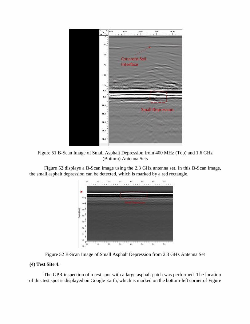
Figure 51 B-Scan Image of Small Asphalt Depression from 400 MHz (Top) and 1.6 GHz

(Bottom) Antenna Sets

Figure 52 displays a B-Scan image using the 2.3 GHz antenna set. In this B-Scan image,

the small asphalt depression can be detected, which is marked by a red rectangle.

Figure 52 B-Scan Image of Small Asphalt Depression from 2.3 GHz Antenna Set

(4) Test Site 4:

The GPR inspection of a test spot with a large asphalt patch was performed. The location

of this test spot is displayed on Google Earth, which is marked on the bottom-left corner of Figure

45. The physical test site picture is shown in Figure 53. The large asphalt patch is marked with a

red curve.

Figure 53 Test Spot with Large Asphalt Patch

The B-Scan images are displayed in Figure 54. In the 400 MHz B-Scan image (the top

image), the subsurface concrete-soil interface was detected at a 26 inch depth. In the 1.6 GHz B-

Scan image (the bottom image), the large asphalt patch was detected, which is marked by a red

rectangle.

Figure 54 B-Scan Image of Large Asphalt Patch from 400 MHz (Top) and 1.6 GHz (Bottom)

Antenna Sets

Figure 55 displays the B-Scan image derived from the 2.3 GHz antenna set. In this B-Scan

image, the large asphalt patch can be detected, which is marked by a red rectangle.

Figure 55 B-Scan Image of Large Asphalt Patch from 2.3 GHz Antenna Set

(5) Test Site 5:

A GPR inspection of a test spot plugged with a concrete drain pipe was performed. The

location of this test spot is marked in red in Figure 56. The physical test site picture is shown in

Figure 57. The asphalt pavement also had small cracks on the surface which can be observed in

Figure 57 (b).

Figure 56 Test Site on Google Earth

Figure 57 (a) Test Spot Plugged with Concrete Drain Pipe;

(b) Asphalt Pavement Crack on the Surface

The B-Scan images are displayed in Figure 58. The hyperbola representing the underground

concrete drain pipe was detected at a 26 inch depth in the 400 MHz B-Scan image (the top image).

Also the subsurface concrete-soil interface can be detected at a 40 inch depth. In the 1.6 GHz B-

Scan image (the bottom image), the cracks on the asphalt pavement surface was detected and

marked by a red rectangle.

Figure 58 B-Scan Image of Underground Concrete Pipe and Surface Asphalt Crack from 400

MHz (Top) and 1.6 GHz (Bottom) Antenna Sets

Figure 59 displays the B-Scan image from the 2.3 GHz antenna set. In this B-Scan image,

the cracks on the asphalt pavement surface can be detected, which is marked by a red rectangle.

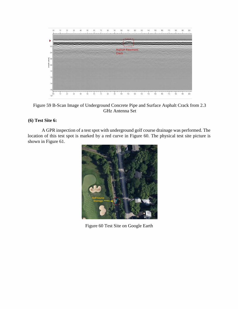
Figure 59 B-Scan Image of Underground Concrete Pipe and Surface Asphalt Crack from 2.3

GHz Antenna Set

(6) Test Site 6:

A GPR inspection of a test spot with underground golf course drainage was performed. The

location of this test spot is marked by a red curve in Figure 60. The physical test site picture is

shown in Figure 61.

Figure 60 Test Site on Google Earth

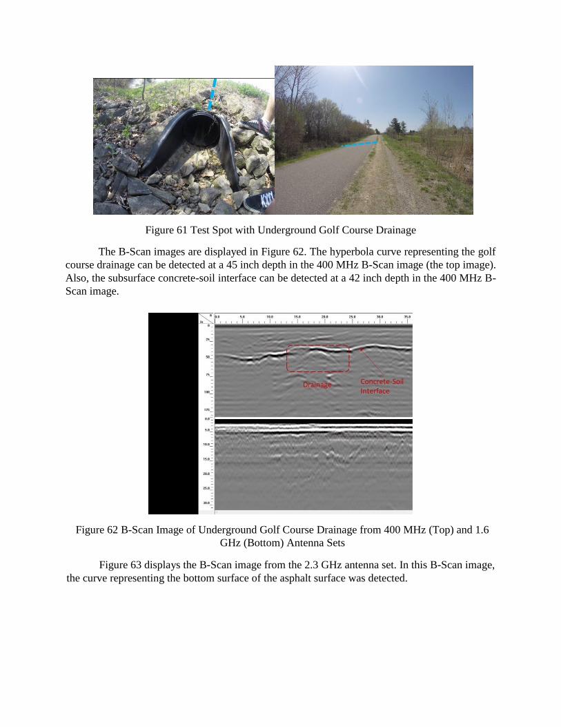
Figure 61 Test Spot with Underground Golf Course Drainage

The B-Scan images are displayed in Figure 62. The hyperbola curve representing the golf

course drainage can be detected at a 45 inch depth in the 400 MHz B-Scan image (the top image).

Also, the subsurface concrete-soil interface can be detected at a 42 inch depth in the 400 MHz B-

Scan image.

Figure 62 B-Scan Image of Underground Golf Course Drainage from 400 MHz (Top) and 1.6

GHz (Bottom) Antenna Sets

Figure 63 displays the B-Scan image from the 2.3 GHz antenna set. In this B-Scan image,

the curve representing the bottom surface of the asphalt surface was detected.

Figure 63 B-Scan Image of Underground Golf Course Drainage from the 2.3 GHz Antenna Set

Chapter 5 Conclusions:

In this project, ground penetrating radar for transportation infrastructure structural

inspections were investigated. The research consisted of three major parts: GPR hardware design

including electronic circuit and mechanical structure; GPR signal processing algorithm and

database design; Field test for function validation and inspection performance assessment.

From a GRP hardware perspective, we are able to complete the high speed GPR circuit and

mechanical design, which is currently ready to be implemented for field inspections. In addition,

a commercial GPR system (GSSI SIR30) was obtained. Design modification has been done to

achieve a dual-band system operable at 400 MHz and 1.6 GHz, which enables the system to have

an inspection depth of over 120 inches.

From a GPR signal processing perspective, algorithms have been developed to extract the

features of interests. Experiments on road pavement inspection were conducted. Also, a GPR data

management database was designed.

A series of field tests were performed, including a road test at St. Paul Street, Burlington,

a road test at the bicycle trail of South Burlington Recreation Path, and many other small scale

tests on the UVM campus. These tests provided valuable information that was used to assess GPR

functions and performance, which was then used to improve our GPR hardware and algorithm

design. With these tests, we are able to develop systematic methodologies that are suitable for large

scale road inspections.

This study has fulfilled the overarching research objective by developing the systematic

methodology of employing GPR, including instruments, subsequent data processing and

interpretation applicable for roadway pavement and bridge inspections. The test methodologies

and the complete set of procedures for applying GPR for surveying the transportation

infrastructural conditions are very well explored and validated. This research has deepen our

understandings of GPR sensing capabilities, and improved our skills of operating GPR systems

and processing GPR data for underground structure sensing. We have a good confidence and strong

wiliness to further our collaborations with VTrans to employ GPR to facilitate transportation

infrastructure survey, maintenance, repair and rehabilitation in Vermont and beyond.

The research has led to several paper publications:

• Ahmed, Y. Zhang, D. Burns, D. Huston, T. Xia, "Design of UWB Antenna for Air Coupled

Impulse Ground Penetrating Radar," IEEE Geoscience and Remote Sensing Letters. Vol. 13,

No. 1. Jan. 2016. pp 92-96.

• Y. Zhang, D. Huston, T. Xia, "Underground Object Characterization based on Neural

Networks for Ground Penetrating Radar Data," in Proceedings of SPIE Smart Structure/NDE

Conference 2016.

• M. Matwally, N. Esperance, T. Xia, "Ground Penetrating Radar Utilizing Compressive

Sampling and OFDM Techniques," in Proceedings of IEEE International Symposium on

Circuits and Systems (ISCAS), 2015.

• Y, Zhang, D. Burns, D. Huston, T. Xia, "Sand Moisture Assessment using Instantaneous Phase

Information in Ground Penetrating Radar Data", in Proceedings of SPIE Smart

Structures/NDE Conference 2015.