Embed Size (px)
Citation preview

Hindawi Publishing CorporationEURASIP Journal on Advances in Signal ProcessingVolume 2010, Article ID 205095, 13 pagesdoi:10.1155/2010/205095
Review Article
High-Resolution Sonars: What Resolution DoWeNeed forTarget Recognition?
Yan Pailhas, Yvan Petillot, and Chris Capus
School of Electrical and Physical Science, Oceans Systems Laboratory, Heriot Watt University, Edinburgh EH14 4AS, Scotland, UK
Correspondence should be addressed to Yan Pailhas, [email protected]
Received 23 December 2009; Revised 28 July 2010; Accepted 1 December 2010
Academic Editor: Yingzi Du
Copyright © 2010 Yan Pailhas et al. This is an open access article distributed under the Creative Commons Attribution License,which permits unrestricted use, distribution, and reproduction in any medium, provided the original work is properly cited.
Target recognition in sonar imagery has long been an active research area in the maritime domain, especially in the mine-countermeasure context. Recently it has received even more attention as new sensors with increased resolution have been developed;new threats to critical maritime assets and a new paradigm for target recognition based on autonomous platforms have emerged.With the recent introduction of Synthetic Aperture Sonar systems and high-frequency sonars, sonar resolution has dramaticallyincreased and noise levels decreased. Sonar images are distance images but at high resolution they tend to appear visually as opticalimages. Traditionally algorithms have been developed specifically for imaging sonars because of their limited resolution and highnoise levels. With high-resolution sonars, algorithms developed in the image processing field for natural images become applicable.However, the lack of large datasets has hampered the development of such algorithms. Here we present a fast and realistic sonarsimulator enabling development and evaluation of such algorithms. We develop a classifier and then analyse its performancesusing our simulated synthetic sonar images. Finally, we discuss sensor resolution requirements to achieve effective classification ofvarious targets and demonstrate that with high resolution sonars target highlight analysis is the key for target recognition.
1. Introduction
Target recognition in sonar imagery has long been an activeresearch area in the maritime domain. Recently, however,it has received increased attention, in part due to thedevelopment of new generations of sensors with increasedresolution and in part due to the emergence of new threatsto critical maritime assets and a new paradigm for targetrecognition based on autonomous platforms. The recentintroduction of operational Synthetic Aperture Sonar (SAS)systems [1, 2] and the development of ultrahigh resolutionacoustic cameras [3] have increased tenfold the resolution ofthe images available for target recognition as demonstratedin Figure 1. In parallel, traditional dedicated ships arebeing replaced by small, low cost, autonomous platformseasily deployable by any vessel of opportunity. This createsnew sensing and processing challenges, as the classificationalgorithms need to be fully automatic and run in real timeon the platforms. The platforms’ behaviours also requireto be autonomously adapted online, to guarantee appro-priate detection performance is met, sometimes on very
challenging terrains. This creates a direct link between sens-ing and mission planning, sometimes called active percep-tion, where the data acquisition is directly controlled by thescene interpretation.
Detection and identification techniques have tended tofocus on saliency (global rarity or local contrast) [4–6],model-based detection [7–15] or supervised learning [16–22]. Alternative approaches to investigate the internal struc-ture of objects using wideband acoustics [23, 24] are showingsome promises, but it is now widely acknowledged thatcurrent techniques are reaching their limits. Yet, their perfor-mances do not enable rapid and effective mine clearance andfalse alarm rates remain prohibitively high [4–22]. This is nota critical problem when operators can validate the outputs ofthe algorithms directly, as they still enable a very high datacompression rate by dramatically reducing the amount ofinformation that an operator has to review. The increasinguse of autonomous platforms raises fundamentally differentchallenges. Underwater communication is very poor due tothe very low bandwidth of the medium (the data transfer rateis typically around 300 bits/s) and it does not permit online

2 EURASIP Journal on Advances in Signal Processing
(a)
3.5 3.5
3 3
2.5 2.5
(b)
Figure 1: Example of Target in Synthetic Aperture Sonar (a) and Acoustic Camera (b). Images are courtesy of the NATO Undersea ResearchCentre (a) and Soundmetrics Ltd (b).
(a) (b)
(c) (d)
Figure 2: Snapshots of four different types of seabed: (a) flat seabed, (b) sand ripples, (c) rocky seabed and (d) cluttered environment.
operator visualisation or intervention. For this reason theuse of collaborating multiple platforms requires robust andaccurate on-board decision making.
The question of resolution has been raised again bythe advent of very high resolution sidescan, forward-lookand SAS systems. These change the quality of the imagesmarkedly producing near-optical images. This paper looks atwhether the resolution is now high enough to apply opticalimage processing techniques to take advantage of advancesmade in other fields.
In order to improve these performances, the MCM(Mine and Counter Measures) community has focused onimproving the resolution of the sensors and high resolutionsonars are now a reality. However, these sensors are veryexpensive and very limited data (if any) are available to theresearch community. This has hampered the development ofnew algorithms for effective on-board decision making.
In this paper, we present tools and algorithms to ad-dress the challenges for the development of improved target
detection algorithms using high resolution sensors. We focuson two key challenges.
(i) The development of fast simulation tools for highresolution sensors: this will enable us to tackle thecurrent lack of real datasets to develop and evaluatenew algorithms including generative models fortarget identification. It will also provide a ground-truth simulation environment to evaluate potentialactive perception strategies.
(ii) What resolution do we need? The development ofnew sensors has been driven by the need for increasedresolution.
The remainder of the paper is organized as follows: InSection 2, a fast and realistic sonar simulator is described.In Sections 3 and 4, the simulator is used to explore theresolution issue. Its flexibility enables the generation of real-istic sonar images at various resolutions and the exploration

EURASIP Journal on Advances in Signal Processing 3
Figure 3: Decomposition of the 3D representation of the seafloorin 3 layers: partition between the different types of seabed, globalelevation, roughness and texture.
Manta Rockam Cuboid
Hemisphere Cylinder Standing cylinder
Figure 4: 3D models of the different targets and minelike objects.
of the effects of resolution on classification performance.Extensive simulations provide a database of synthetic imageson various seabed types. Algorithms can be developed andevaluated using the database. The importance of the pixelresolution for image-based algorithms is analysed as well asthe amount of information contained in the target shadow.
2. Sidescan Simulator
Sonar images are difficult and expensive to obtain. A realisticsimulator offers an alternative to develop and test MCMalgorithms. High-frequency sonars and SAS increase theresolution of the sonar image from tens of cm to a few cm (3to 5 cm). The resulting sonar images become closer to opticalimages. By increasing the resolution of the image the objectsbecome sharper. Our objective here is to produce a simulatorthat can realistically reproduce such images in real time.
There is an existing body of research into sonarsimulation[25, 26]. The simulators are generally based onray-tracing techniques [27] or on a solution to the full waveequation [28]. SAS simulation takes into account the SAS
SoNaR
d
Bottom
r
dΦ
θ
cτ
2
dA
dA = cτ
2rdΦ
Figure 5: Definitions for surface reverberation modeling.
Startingpoint
Seafloor
Sidescansonar
Finishpoint
Insonified area
Figure 6: The trajectory of the sonar platform can be placed intothe 3D environment.
processing and is, in general, highly complex [26]. Critically,in all cases, the algorithms are extremely slow (one hourto several days to compute a synthetic sidescan image witha desktop computer). When high frequencies are used, thepath of the acoustic waves can be approximated by straightlines. In this case, classical ray-tracing techniques combinedwith a careful and detailed modeling of the energy-basedsonar equation can be used. The results obtained are verysimilar to those obtained using more complex propagationmodels. Yet they are much faster and produce very realisticimages.
Note that this simulator is a high-precision sidescansimulator, which can be equally well applied to forwardlooking sonar. SAS images differ from sidescan images inmainly two points: a constant pixel resolution at all rangesand a blur in the object shadows [29]. The simulator cancope with the constant range resolution so synthetic targethighlights will appear similar. A fully representative SAS

4 EURASIP Journal on Advances in Signal Processing
50
40
30
20
10
0
Cro
ssra
nge
(m)
0 20 40
Range (m)
(a)
50
40
30
20
10
0
Cro
ssra
nge
(m)
0 20 40
Range (m)
(b)
Figure 7: Display of the resulting sidescan images ((a) and (b)) of the same scene with different trajectory. The seafloor is composed with twosand ripples phenomena at different frequencies and different sediments (VeryFineSand for the high frequency ripples and VeryCoarseSandfor the low frequency ripples). A manta object has been put in the centre of the map.
shadow model remains to be implemented, but the analysesare still relevant for identification of targets from highlightsin SAS imagery.
The simulator presented here first generates a realisticsynthetic 3D environment. The 3D environment is dividedinto three layers: a partition layer which assigns a seabed typeto each area, an elevation profile corresponding to the generalvariation of the seabed, and a 3D texture that models eachseabed structure. Figure 2 displays snapshots of four differenttypes of seabed (flat sediment, sand ripples, rocky seabedand a cluttered environment) that can be generated by thesimulator. All these natural structures can be well modeledusing fractal representations. The simulator can also takeinto account various compositions of the seabed in termsof scattering strengths. The boundaries between each seabedtype are also modeled using fractals.
Objects of different shapes and different materials canbe inserted into the environment. For MCM algorithms,several types of mines have been modeled such as the Manta(truncated cone shape), Rockan and cylindrical mines.
The resulting 3D environment is an heightmap, meaningthat to one location corresponds one unique elevation. Soobjects floating in midwater for example cannot be modelledhere.
The sonar images are produced from this 3D environ-ment, taking into account a particular trajectory of thesensor (mounted on a vessel or an autonomous platforms).The seabed reflectivity is computed thanks to state-of-the-art models developed by APL-UW in the High-FrequencyOcean Environmental Acoustic Models Handbook [30] andthe reflectivity of the targets is based on a Lambertianmodel. A pseudo ray-tracing algorithm is performed andthe sonar equation is solved for each insonified area giving
the backscattered energy. Note that the shadows are auto-matically taken into account thanks to the pseudo ray-tracingalgorithm. The processing time required to compute a sonarimage of 50 m by 50 m using a 2 GHz Intel Core 2 Duo with2 GB of memory is approximately 7 seconds. The remainderof the section details each of the modules required to performthe simulation.
2.1. 3D Digital Terrain Model Generator. The aim of thismodule is to generate realistic 3D seabed environments. Itshould be able to handle several types of seabed, to generatea realistic model for each seabed type, and to synthesizea realistic 3D elevation. For these reasons, the final 3Dstructure is built by superposition of three different layers: apartition layer, an elevation layer and a texture layer. Figure 3shows an example of the three different layers which form thefinal 3D environment.
In the late seventies, mathematicians such as Mandelbrot[31] linked the symmetry patterns and self-similarity foundin nature to mathematical objects called fractals [32–35].Fractals have been used to model realistic textures andheightmap terrains [33]. A quick way to generate realistic 3Dfractal heightmap terrains is by using a pink noise generator[33]. A pink noise is characterized by its power spectraldensity decreasing as 1/ f β, where 1 < β < 2.
2.1.1. The Partition Layer. In the simulator, various types ofseabeds can be chosen (up to three for a given image). Theboundaries between the seabed types are computed usingfractal borders.
2.1.2. Elevation Layer. This layer contains two types of pos-sible elevation: a linear slope characterizing coastal seabeds

EURASIP Journal on Advances in Signal Processing 5
50
40
30
20
10
0
Cro
ssra
nge
(m)
0 20 40
Range (m)
(a)
50
40
30
20
10
0
Cro
ssra
nge
(m)
0 20 40
Range (m)
(b)
50
40
30
20
10
0
Cro
ssra
nge
(m)
0 20 40
Range (m)
(c)
Figure 8: Examples of simulated sonar images for different seabed types (clutter, flat, ripples), 3D elevation and scattering strength. (a)represents a smooth seabed with some small variations, (b) represents a mixture of flat and cluttered seabed and (c) represents a rippledseabed.
and a random 3D elevation. The random elevation is asmoothing of a pink noise process. The β parameter is usedto tune the roughness of the seabed.
2.1.3. Texture Layer. Four different textures have been cre-ated to model four kinds of seabed. Once again the texturesare synthesized by fractal models derived from pink noisemodels.
(a) Flat Seabed. A simple flat floor is used for the flat seabed.No texture is needed in this case. Differences in reflectivityand scattering between sediment types are handled by theImage Generator module.
(b) Sand Ripples. The sand ripples are characterized by theperiodicity and the direction of the ripples. A modifiedpink noise is used here. In this case the frequency decay isanisotropic. The amplitude of the magnitude of the Fouriertransform follows (1). The frequency of the ripples is given
by Fripples =√f 2xpeak + f 2
ypeak and the direction is given by
θ = tan−1( fxpeak/ fypeak). The phase is modeled by a uniformdistribution
F(fx, fy
)= 1(fx − fxpeak
)β1
(fy − fypeak
)β . (1)
(c) Rocky Seabed. The magnitude of the Fourier transformof the the rocky seabed is modeled by (2). The factor α

6 EURASIP Journal on Advances in Signal Processing
0
0.2
0.4
0.6
0.8
1
1.2
1.4Comparison of leading side-scan sonars for MCM
Cov
erag
era
te(n
M/h
)
0 0.2 0.4 0.6 0.8 1
Along track resolution of the sonar (m)
EdgeTech 4200 MPXKlein 5000-455Klein 3000-500EdgeTech 4200-600Typical SASMilitary SAS
Identification rangeDetection rangeKlein 5000-455
Figure 9: Ability to detect and identify targets as a function ofresolution and coverage rate (Nm/h: nautical mile per hour) for thebest sidescan and synthetic aperture sonars. The SAS sonars hereare a typical 100–300 kHz sonar in optimal conditions for syntheticaperture.
models the anisotropic erosion of the rock due to underwatercurrents
F(fx, fy
)= 1(√
α · f 2x + f 2
y
)β ,(2)
(d) Cluttered Environment. The cluttered environment ischaracterized by a random distribution of small rocks.A poisson distribution has been chosen for the spatialdistribution of the rocks on the seabed as the mean numberof occurrences is relatively small.
2.2. Targets. A separate module is provided for adding targetsinto the environment. Figure 4 displays the 3D models of 6different targets. Location, size and material composition canbe adjusted by the user. The resulting sidescan images offer alarge data base for detection and classification algorithms.
Nonmine targets can also be generated by varyingparameters in this module. Several are used to test thealgorithms with results presented in Section 4.1.2.
2.3. The Sonar Image Generator. The sonar module computesthe sidescan image from a given 3D environment. Thesimulator is ray-tracing-based and solves the sonar equation[36] (given in (3)). Because (3) is an energetic equation,phenomena such as multipaths are not taken into account.
For a monostatic sonar system, the sound propagation canbe expressed from an energetic point of view as
XS = SL− 2TL + TS + DI−NL− RL, (3)
where XS is the excess level, that is, the backscattering energy,SL is the Source Level of the projector, DI is the DirectivityIndex, TL is the Transmission Loss, NL is the Noise Level, RLis the Reverberation Level and TS is the Target Strength. Allthe parameters are measured in decibels (dB) relative to thestandard reference intensity of a 1 μPa plane wave.
In a wide range of cases, a good approximation totransmission loss TL can be made by considering the processas a combination of free field spherical spreading and anadded absorption loss. This working rule can be expressedas
TL = 20 log r + αr, (4)
where r is the transmission range and α is an attenuationcoefficient expressed in dB/m. The attenuation coefficientcan be expressed as the sum of two chemical relaxation pro-cesses and the absorption of pure water. It can be computednumerically thanks to the Francois-Garrison formula [37].
Reverberation Level is an important restricting factor inthe detection process, especially in the context of MCM. Atshort ranges, it represents the most significant noise factor.The surface reverberation can be developed as drawn inFigure 5, where dA defines the elementary surface subtendedby horizontal angle dφ and is dependent on the pulse lengthτ and range. Returns from the front and rear ends of thepulse determine the size of the elementary surface element,dA. So, for the seabed contribution to reverberation level, wecan write
RL = SL− 2TL + Ss + 10 logcτ
2φr, (5)
where d is the altitude of the sonar, r is the range to theseabed along the main axis of the transducer beam and t istime.
Three types of seabed have been implemented: RoughRock, Sandy Gravel and Very Fine Sand. A theoretical BottomScattering Strength (Ss in (5)) can be computed thanks to[30].
The source level SL is the power of the transmitter. It is aconstant and given by the sonar manufacturer. For sidescanthe SL is typically between 200 and 230 dB.
The Directivity Index (DI) is a sonar-dependent factorassociated with directionality of the transducer system. Thesimulator includes a simple beam pattern derived from acontinuous line array model of length l. The beam patternfunction can be computed thanks to the following:
B(θ) =[
sin(πl/λ) sin θ(πl/λ) sin θ
]. (6)
Also any transducer beam pattern can be integrated intothe simulator.
In our model, the targets form part of the 3D envi-ronment. The Target Scattering Strength (TS) is computed
EURASIP Journal on Advances in Signal Processing 7
3
2
1
0
(Met
ers)
0 1 2 3
(Meters)
(a)
3
2
1
0
(Met
ers)
0 1 2 3
(Meters)
(b)
3
2
1
0
(Met
ers)
0 1 2 3
(Meters)
(c)
3
2
1
0
(Met
ers)
0 1 2 3
(Meters)
(d)
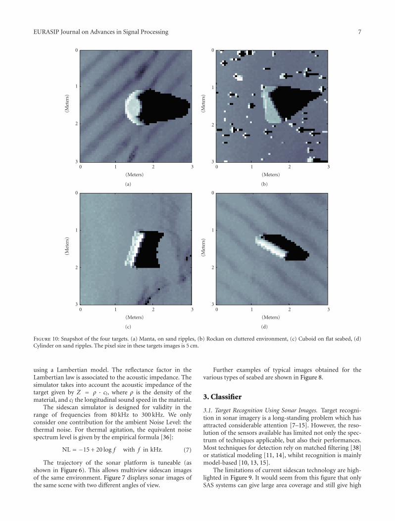
Figure 10: Snapshot of the four targets. (a) Manta, on sand ripples, (b) Rockan on cluttered environment, (c) Cuboid on flat seabed, (d)Cylinder on sand ripples. The pixel size in these targets images is 5 cm.
using a Lambertian model. The reflectance factor in theLambertian law is associated to the acoustic impedance. Thesimulator takes into account the acoustic impedance of thetarget given by Z = ρ · cl, where ρ is the density of thematerial, and cl the longitudinal sound speed in the material.
The sidescan simulator is designed for validity in therange of frequencies from 80 kHz to 300 kHz. We onlyconsider one contribution for the ambient Noise Level: thethermal noise. For thermal agitation, the equivalent noisespectrum level is given by the empirical formula [36]:
NL = −15 + 20 log f with f in kHz. (7)
The trajectory of the sonar platform is tuneable (asshown in Figure 6). This allows multiview sidescan imagesof the same environment. Figure 7 displays sonar images ofthe same scene with two different angles of view.
Further examples of typical images obtained for thevarious types of seabed are shown in Figure 8.
3. Classifier
3.1. Target Recognition Using Sonar Images. Target recogni-tion in sonar imagery is a long-standing problem which hasattracted considerable attention [7–15]. However, the reso-lution of the sensors available has limited not only the spec-trum of techniques applicable, but also their performances.Most techniques for detection rely on matched filtering [38]or statistical modeling [11, 14], whilst recognition is mainlymodel-based [10, 13, 15].
The limitations of current sidescan technology are high-lighted in Figure 9. It would seem from this figure that onlySAS systems can give large area coverage and still give high
8 EURASIP Journal on Advances in Signal Processing
0
10
20
30
40
50
60
70
Mis
iden
tifi
cati
on(%
)
5 10 15 20 25 30
Pixel resolution (cm)
MantaRockan
CylinderCube
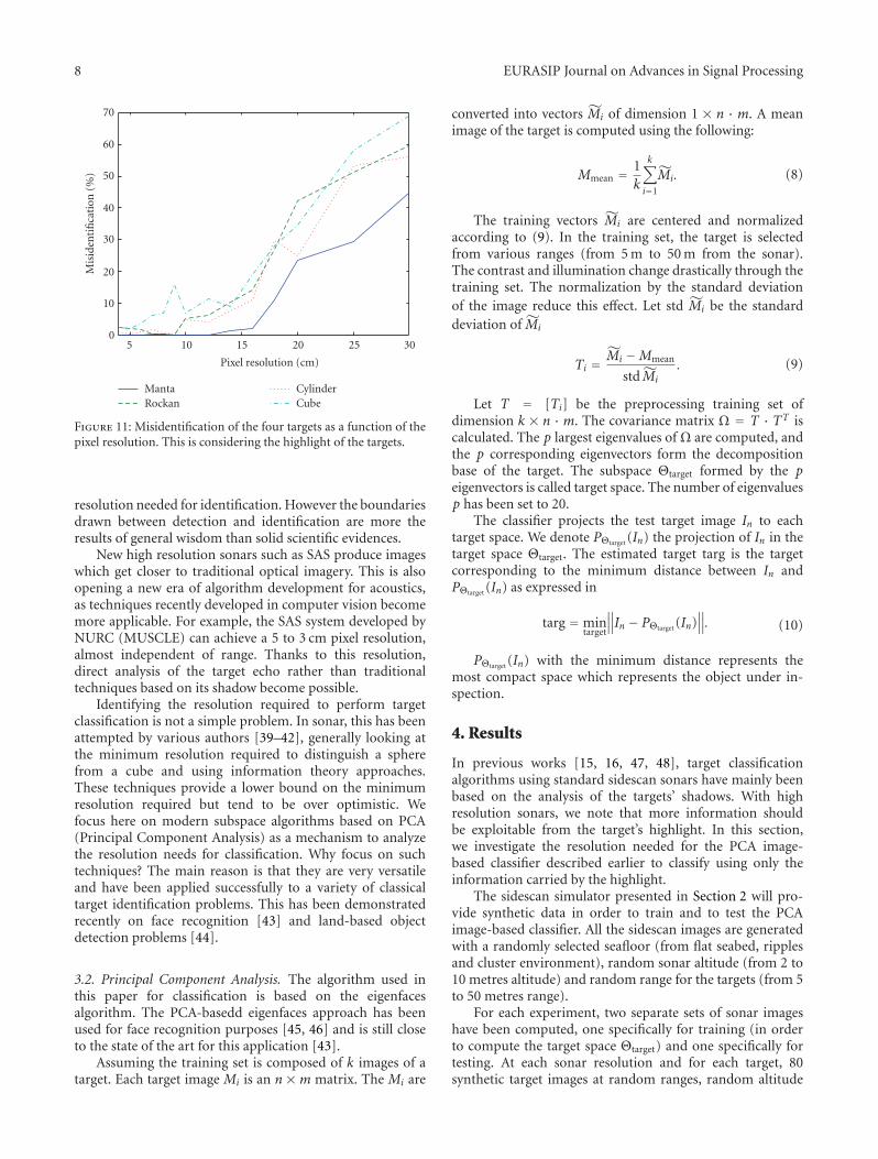
Figure 11: Misidentification of the four targets as a function of thepixel resolution. This is considering the highlight of the targets.
resolution needed for identification. However the boundariesdrawn between detection and identification are more theresults of general wisdom than solid scientific evidences.
New high resolution sonars such as SAS produce imageswhich get closer to traditional optical imagery. This is alsoopening a new era of algorithm development for acoustics,as techniques recently developed in computer vision becomemore applicable. For example, the SAS system developed byNURC (MUSCLE) can achieve a 5 to 3 cm pixel resolution,almost independent of range. Thanks to this resolution,direct analysis of the target echo rather than traditionaltechniques based on its shadow become possible.
Identifying the resolution required to perform targetclassification is not a simple problem. In sonar, this has beenattempted by various authors [39–42], generally looking atthe minimum resolution required to distinguish a spherefrom a cube and using information theory approaches.These techniques provide a lower bound on the minimumresolution required but tend to be over optimistic. Wefocus here on modern subspace algorithms based on PCA(Principal Component Analysis) as a mechanism to analyzethe resolution needs for classification. Why focus on suchtechniques? The main reason is that they are very versatileand have been applied successfully to a variety of classicaltarget identification problems. This has been demonstratedrecently on face recognition [43] and land-based objectdetection problems [44].
3.2. Principal Component Analysis. The algorithm used inthis paper for classification is based on the eigenfacesalgorithm. The PCA-basedd eigenfaces approach has beenused for face recognition purposes [45, 46] and is still closeto the state of the art for this application [43].
Assuming the training set is composed of k images of atarget. Each target image Mi is an n ×m matrix. The Mi are
converted into vectors Mi of dimension 1 × n · m. A meanimage of the target is computed using the following:
Mmean = 1k
k∑
i=1
Mi. (8)
The training vectors Mi are centered and normalizedaccording to (9). In the training set, the target is selectedfrom various ranges (from 5 m to 50 m from the sonar).The contrast and illumination change drastically through thetraining set. The normalization by the standard deviationof the image reduce this effect. Let std Mi be the standarddeviation of Mi
Ti = Mi −Mmean
std Mi
. (9)
Let T = [Ti] be the preprocessing training set ofdimension k × n · m. The covariance matrix Ω = T · TT iscalculated. The p largest eigenvalues of Ω are computed, andthe p corresponding eigenvectors form the decompositionbase of the target. The subspace Θtarget formed by the peigenvectors is called target space. The number of eigenvaluesp has been set to 20.
The classifier projects the test target image In to eachtarget space. We denote PΘtarget (In) the projection of In in thetarget space Θtarget. The estimated target targ is the targetcorresponding to the minimum distance between In andPΘtarget (In) as expressed in
targ = mintarget
∥∥∥In − PΘtarget (In)∥∥∥. (10)
PΘtarget (In) with the minimum distance represents themost compact space which represents the object under in-spection.
4. Results
In previous works [15, 16, 47, 48], target classificationalgorithms using standard sidescan sonars have mainly beenbased on the analysis of the targets’ shadows. With highresolution sonars, we note that more information shouldbe exploitable from the target’s highlight. In this section,we investigate the resolution needed for the PCA image-based classifier described earlier to classify using only theinformation carried by the highlight.
The sidescan simulator presented in Section 2 will pro-vide synthetic data in order to train and to test the PCAimage-based classifier. All the sidescan images are generatedwith a randomly selected seafloor (from flat seabed, ripplesand cluster environment), random sonar altitude (from 2 to10 metres altitude) and random range for the targets (from 5to 50 metres range).
For each experiment, two separate sets of sonar imageshave been computed, one specifically for training (in orderto compute the target space Θtarget) and one specifically fortesting. At each sonar resolution and for each target, 80synthetic target images at random ranges, random altitude

EURASIP Journal on Advances in Signal Processing 9
1.2
1
0.8
0.6
0.4
0.2(M
eter
s)
0.2 0.4 0.6 0.8 1 1.2
(Meters)
Manta
(a)
1.2
1
0.8
0.6
0.4
0.2
0.2 0.4 0.6 0.8 1 1.2
(Meters)
Rockan
(b)
1.2
1
0.8
0.6
0.4
0.2
0.2 0.4 0.6 0.8 1 1.2
(Meters)
Cylinder
(c)
1.2
1
0.8
0.6
0.4
0.2
(Met
ers)
0.2 0.4 0.6 0.8 1 1.2
(Meters)
Cuboid
(d)
1.2
1
0.8
0.6
0.4
0.2
0.2 0.4 0.6 0.8 1 1.2
(Meters)
Big hemisphere
(e)
1.2
1
0.8
0.6
0.4
0.2
0.2 0.4 0.6 0.8 1 1.2
(Meters)
Hemisphere
(f)
1.2
1
0.8
0.6
0.4
0.2
0.2 0.4 0.6 0.8 1 1.2
(Meters)
Box
(g)
Figure 12: Snapshot of the targets used for classification. On the first line, the minelike targets with the Manta, the Rockan and the cylinder.On the second line, the nonmine targets with the cube, the two hemispheres, and the box shape target. The pixel size in these targets imagesis 5 cm.
0
0.2
0.4
0.6
0.8
1
0.05 0.1 0.15 0.2 0.25 0.3
Mis
iden
tifi
cati
on(%
)
Pixel resolution (m)
BoxCubeCylinderHemisphere
Small hemisphereMantaRockan
(a)
0
0.2
0.4
0.6
0.8
1
0.05 0.1 0.15 0.2 0.25 0.3
Mis
clas
sifi
cati
on(%
)
Pixel resolution (m)
Mine-like objectNon mine object
(b)
Figure 13: (a) Misidentification of the seven targets as a function of the pixel resolution. (b) Misclassification of the target as function of thepixel resolution.

10 EURASIP Journal on Advances in Signal Processing
Figure 14: Snapshot of the shadow of the four targets (from left toright: Manta, Rockan, Cube and Cylinder) to classify with differentorientations and backgrounds. The pixel size is these target imagesis 5 cm. The size of each snapshot is 1.25 m × 2.75 m.
0
10
20
30
40
50
0.05 0.1 0.15 0.2 0.25 0.3
Mis
iden
tifi
cati
on(%
)
Pixel resolution (cm)
MantaRockan
CylinderCube
Figure 15: Percentage of misidentification versus the pixel resolu-tion for various target types. This considers the shadow of the targetand not its echo.
and with a randomly selected seafloor have been used fortraining. A larger set of 40000 synthetic target images areused to test the classifier. The classifier is trained and testedaccording to the algorithm described in Section 3.2.
4.1. What Precision Is Needed?
4.1.1. Identification. In this first experiment the PCA clas-sifier is train for identification. Assuming a minelike objecthas been detected and classified as a mine, the algorithmidentifies the kind of mine the target Four targets have beenchosen: a Manta mine (truncated cone with dimensions98 cm lower diameter; 49 cm upper diameter; 47 cm height),a Rockan mine (L × W × H: 100 cm × 50 cm × 40 cm),a cuboid with dimensions 100 cm × 30 cm × 30 cm and acylinder 100 cm long and 30 cm in diameter.
Figure 10 displays snapshots of the four different targetsfor a 5 cm sonar resolution.
The pixel resolution is tunable in the simulator. Sidescansimulation/classification processes have been run for 15different pixel resolutions from 3 cm (high resolution sonar)to 30 cm (low resolution sonar) covering the detection andclassification range of side looking sonars. Figure 11 displaysthe misidentification % of the four targets against the pixelresolution.
As expected, the image-based classifier fails at low resolu-tions. Between 15 and 20 cm resolution, which correspondsto the majority of standard sonar systems, classification basedon the highlights is poor (between 50% and 80% correctclassification). The results stabilize at around 5 cm resolutionto reach around 95% correct classification.
In previous work involving face recognition where ithas been shown that PCA techniques are not very robustto rotation [49]. The algorithm can be optimized usingmultiple subspaces for each nonsymmetric target, each of thesubspaces covering a limited angular range.
4.1.2. Classification. In this section we extend the PCAclassifier for underwater object classification purposes. Alarger set of seven targets have been chosen with threeminelike objects: the Manta, the Rockan, a cylinder 100 cmlong and 30 cm diameter and four nonmine objects: a cuboidwith dimension 100 cm × 50 cm × 40 cm, two hemisphereswith diameters, respectively, 100 cm and 50 cm and a boxwith dimension 70 cm × 70 cm × 40 cm. Note that thenonmine targets have been chosen such as the dimensionof the big hemisphere matches with the dimension of theManta, and the dimension of the box matches with thedimension of the Rockan. Figure 12 provides snapshots ofthe different targets.
As described in Section 4.1.1, two data sets for trainingand testing have been produced. The target classificationrelies on two steps: at first the target is identify followingthe same process as Section 4.1.1 and then classified into twoclasses minelike and nonmine
Figure 13(a) displays the results of the identification step.the curves of misidentification for each target follow thegeneral pattern described earlier in Section 4.1.1 with a lowmisidentification (below 5%) for a pixel resolution lowerthan 5 cm. In Figure 13(b), the results of the classificationbetween minelike and nonmine is showed. Contrary to theidentification process, the classification curves stabilise athigher pixel resolution (around 10 cm) to 2-3% misclassifi-cation.
In these examples we show that the identification taskneeds a higher pixel resolution that the classification taskto match the same performances 95% correct identifica-tion/classification.
4.2. Identification with Shadow. As mentioned earlier, cur-rent sidescan ATR algorithms depend strongly on thetarget shadow for detection and classification. The usualassumption made is: at low resolution the information relativeto the target is mostly contained in its shadow. In this sectionwe aim to confirm this statement by using the classifierdescribed in Section 3.2 directly on the target shadows.

EURASIP Journal on Advances in Signal Processing 11
We study here the quantity of information containedinto the shape of the shadow, and how this information isretrievable depending on the pixel resolution.
Shadows are the result of the directional acoustic illumi-nation of a 3D target. They are therefore range dependent.For the purposes of this experiment, in order to remove theeffect of the range dependence of the shadows, the targetsare positioned at a fixed range of 25 m from the sensor.Image segments containing the target shadows are extractedfrom the data. Figure 14 displays snapshots of target shadowswith different orientations and backgrounds for a 5 cm pixelresolution. We process the target shadow images in exactlyin the same way as we did for the target highlight imagesin the previous sections. For each sonar resolution, 80 targetshadows per object are used for training the classifier, and aset of 40000 shadow images is used for testing.
In total 15 training/classification simulations have beendone for 15 sonar pixel resolutions (from 5 cm to 30 cm).Figure 15 shows the percentage of misclassification versus thepixel resolution for various target types.
Concerning the Cylinder and Cuboid targets, their shad-ows are very similar due the similar geometry. In Figure 14it is almost impossible to distinguish visually between thetwo objects looking only at their shadows. In broadside forexample, the two shadows have exactly the same rectangularshape, explaining why the confusion between these twoobjects is high.
For the Manta and Rockan targets, the misidentificationcurves stabilize near 0% misidentification below 20 cm sonarresolution. Therefore, for standard sidescan systems with aresolution in the 10–30 cm range, the target information canbe extracted from the shadow with an excellent probability ofcorrect identification. In comparison, correct identificationusing the target highlights at 20 cm resolution is about 50%(cf. Figure 11)
5. Conclusions and FutureWork
In this paper, a new real-time realistic sidescan simulator hasbeen presented. Thanks to the flexibility of this numericaltool, realistic synthetic data can be generated at different pixelresolutions. A subspace target identification technique basedon PCA has been developed and used to evaluate the abilityof modern sonar systems to identify a variety of targets.
The results processing shadow images back up the widelyaccepted idea that identification from current sonars at10–20 cm resolution is reaching its performance limit. Theadvent of much higher resolution sonars has now made itpossible to bring in and apply techniques new to the fieldfrom optical image processing. The PCA analyses presentedhere, operating on highlight as opposed solely to shadow,show that these can give a significant improvement in targetidentification and classification performance opening theway for reinvigorated effort in this area.
The emergence of very high resolution sonar systemssuch as SAS and acoustic cameras will enable more advancedtarget identification techniques to be used very soon. Thenext phase of this work will be to validate and confirm these
using real SAS data. We are currently undertaking this phasein collaboration with the NATO Undersea Research Centreand DSTL under the UK Defense Research Centre program.
Acknowledgments
This work was supported by EPSRC and DSTL underresearch contracts EP/H012354/1 and EP/F068956/1. Theauthors also acknowledge support from the Scottish FundingCouncil for the Joint Research Institute in Signal and ImageProcessing between the University of Edinburgh and Heriot-Watt University which is a part of the Edinburgh ResearchPartnership in Engineering and Mathematics (ERPem).
References
[1] A. Bellettini, “Design and experimental results of a 300-kHz synthetic aperture sonar optimized for shallow-wateroperations,” IEEE Journal of Oceanic Engineering, vol. 34, no.3, pp. 285–293, 2009.
[2] B. G. Ferguson and R. J. Wyber, “Generalized frameworkfor real aperture, synthetic aperture, and tomographic sonarimaging,” IEEE Journal of Oceanic Engineering, vol. 34, no. 3,pp. 225–238, 2009.
[3] E. O. Belcher, D. C. Lynn, H. Q. Dinh, and T. J. Laughlin,“Beamforming and imaging with acoustic lenses in small,high-frequency sonars,” in Proceedings of the Oceans Confer-ence, pp. 1495–1499, September 1999.
[4] A. Goldman and I. Cohen, “Anomaly subspace detectionbased on a multi-scale Markov random field model,” SignalProcessing, vol. 85, no. 3, pp. 463–479, 2005.
[5] F. Maussang, J. Chanussot, A. Hetet, and M. Amate, “Higher-order statistics for the detection of small objects in a noisybackground application on sonar imaging,” EURASIP Journalon Advances in Signal Processing, vol. 2007, Article ID 47039,17 pages, 2007.
[6] B. R. Calder, L. M. Linnett, and D. R. Carmichael, “Spatialstochastic models for seabed object detection,” in Detectionand Remediation Technologies for Mines and Minelike TargetsII, Proceeding of SPIE, pp. 172–182, April 1997.
[7] M. Mignotte, C. Collet, P. Perez, and P. Bouthemy, “Hybridgenetic optimization and statistical model-based approach forthe classification of shadow shapes in sonar imagery,” IEEETransactions on Pattern Analysis and Machine Intelligence, vol.22, no. 2, pp. 129–141, 2000.
[8] B. Calder, Bayesian spatial models for sonar image interpre-tation, Ph.D. dissertation, Heriot-Watt University, September1997.
[9] G. J. Dobeck, J. C. Hyland, and LE. D. Smedley, “Automateddetection and classification of sea mines in sonar imagery,” inDetection and Remediation Technologies for Mines andMinelikeTargets II, Proceedings of SPIE, pp. 90–110, April 1997.
[10] I. Quidu, J. PH. Malkasse, G. Burel, and P. Vilbe, “Mineclassification based on raw sonar data: an approach combiningFourier descriptors, statistical models and genetic algorithms,”in Proceedings of the Oceans Conference, pp. 285–290, Septem-ber 2000.
[11] B. R. Calder, L. M. Linnett, and D. R. Carmichael, “Bayesianapproach to object detection in sidescan sonar,” IEE Proceed-ings: Vision, Image and Signal Processing, vol. 145, no. 3, pp.221–228, 1998.

12 EURASIP Journal on Advances in Signal Processing
[12] R. Balasubramanian and M. Stevenson, “Pattern recogni-tion for underwater mine detection,” in Proceedings of theComputer-Aided Classification/Computer-Aided Design Confer-ence, Halifax, Canada, November 2001.
[13] S. Reed, Y. Petillot, and J. Bell, “Automated approach toclassification of mine-like objects in sidescan sonar usinghighlight and shadow information,” IEE Proceedings: Radar,Sonar and Navigation, vol. 151, no. 1, pp. 48–56, 2004.
[14] S. Reed, Y. Petillot, and J. Bell, “Model-based approach tothe detection and classification of mines in sidescan sonar,”Applied Optics, vol. 43, no. 2, pp. 237–246, 2004.
[15] E. Dura, J. Bell, and D. Lane, “Superellipse fitting for therecovery and classification of mine-like shapes in sidescansonar images,” IEEE Journal of Oceanic Engineering, vol. 33,no. 4, pp. 434–444, 2008.
[16] B. Zerr, E. Bovio, and B. Stage, “Automatic mine classi-fication approach based on auv manoeuverability and thecots side scan sonar,” in Proceedings of the AutonomousUnderwater Vehicle and Ocean Modelling Networks Conference(GOATS ’00), pp. 315–322, 2001.
[17] M. Azimi-Sadjadi, A. Jamshidi, and G. Dobeck, “Adaptiveunderwater target classification with multi-aspect decisionfeedback,” in Proceedings of the Computer-Aided Classification/Computer-Aided Design Conference, Halifax, Canada, Novem-ber 2001.
[18] I. Quidu, J. PH. Malkasse, G. Burel, and P. Vilbe, “Mineclassification using a hybrid set of descriptors,” in Proceedingsof the Oceans Conference, pp. 291–297, September 2000.
[19] J. Fawcett, “Image-based classification of side-scan sonardetections,” in Proceedings of the Computer-Aided Classifi-cation/Computer-Aided Design Conference, Halifax, Canada,November 2001.
[20] S. Perry and L. Guan, “Detection of small man-made objectsin multiple range sector scan imagery using neural networks,”in Proceedings of the Computer-Aided Classification/Computer-Aided Design Conference, Halifax, Canada, November 2001.
[21] C. Ciany and W. Zurawski, “Performance of computer aideddetection/computer aided classification and data fusionalgorithms for automated detection and classification ofunderwater mines,” in Proceedings of the Computer-AidedClassification/Computer-Aided Design Conference, Halifax,Canada, November 2001.
[22] C. M. Ciany and J. Huang, “Computer aided detec-tion/computer aided classification and data fusion algorithmsfor automated detection and classification of underwatermines,” in Proceedings of the Oceans Conference, pp. 277–284,September 2000.
[23] Y. Pailhas, C. Capus, K. Brown, and P. Moore, “Analysis andclassification of broadband echoes using bio-inspired dolphinpulses,” Journal of the Acoustical Society of America, vol. 127,no. 6, pp. 3809–3820, 2010.
[24] C. Capus, Y. Pailhas, and K. Brown, “Classification of bottom-set targets from wideband echo responses to bio-inspiredsonar pulses,” in Proceedings of the 4th International Conferenceon Bio-acoustics, 2007.
[25] J. Bell, A model for the simulation of sidescan sonar, Ph.D.dissertation, Heriot-Watt University, August 1995.
[26] A. J. Hunter, M. P. Hayes, and P. T. Gough, “Simulation ofmultiple-receiver, broadband interferometric SAS imagery,”in Proceeding of IEEE Oceans Conference, pp. 2629–2634,September 2003.
[27] J. M. Bell, “Application of optical ray tracing techniques to thesimulation of sonar images,” Optical Engineering, vol. 36, no.6, pp. 1806–1813, 1997.
[28] G. R. Elston and J. M. Bell, “Pseudospectral time-domainmodeling of non-Rayleigh reverberation: synthesis and statis-tical analysis of a sidescan sonar image of sand ripples,” IEEEJournal of Oceanic Engineering, vol. 29, no. 2, pp. 317–329,2004.
[29] M. Pinto, “Design of synthetic aperture sonar systems forhigh-resolution seabed imaging,” in Proceedings of MTS/IEEEOceans Conference, Boston, Mass, USA, 2006.
[30] A. P. L. at the University of Washington, “High-FrequencyOcean Environmental Acoustic Models Handbook,” Tech.Rep. APLUW TR 9407, October 1994.
[31] B. Mandelbrot, The Fractal Geometry of Nature, W. H. Free-man, 1982.
[32] A. P. Pentland, “Fractal-based description of natural scenes,”IEEE Transactions on Pattern Analysis andMachine Intelligence,vol. 6, no. 6, pp. 661–674, 1984.
[33] R. F. Voss, Random Fractal Forgeries in Fundamental Algo-rithms for Computer Graphics, R. A. Earnshaw, Ed., Springer,Berlin, Germany, 1985.
[34] P. A. Burrough, “Fractal dimensions of landscapes and otherenvironmental data,” Nature, vol. 294, no. 5838, pp. 240–242,1981.
[35] S. Lovejoy, “Area-perimeter relation for rain and cloud areas,”Science, vol. 216, no. 4542, pp. 185–187, 1982.
[36] R. J. Urick, Principles of Underwater Sound, McGraw-Hill, NewYork, NY, USA, 3rd edition, 1975.
[37] R. E. Francois, “Sound absorption based on ocean measure-ments: Part I: pure water and magnesium sulfate contribu-tions,” The Journal of the Acoustical Society of America, vol. 72,no. 3, pp. 896–907, 1982.
[38] T. Aridgides, M. F. Fernandez, and G. J. Dobeck, “Adaptivethree-dimensional range-crossrange-frequency filter process-ing string for sea mine classification in side scan sonarimagery,” in Detection and Remediation Technologies for Minesand Minelike Targets II, Proceedings of SPIE, pp. 111–122,April 1997.
[39] M. Pinto, “Performance index for shadow classification inminehunting sonar,” in Proceedings of the UDT Conference,1997.
[40] V. Myers and M. Pinto, “Bounding the performance ofsidescan sonar automatic target recognition algorithms usinginformation theory,” IET Radar, Sonar and Navigation, vol. 1,no. 4, pp. 266–273, 2007.
[41] R. T. Kessel, “Estimating the limitations that image resolutionand contrast place on target recognition,” in Automatic TargetRecognition XII, Proceedings of SPIE, pp. 316–327, usa, April2002.
[42] F. Florin, F. Van Zeebroeck, I. Quidu, and N. Le Bouffant,“Classification performance of minehunting sonar: theory,practical, results and operational applications,” in Proceeedingsof the UDT Conference, 2003.
[43] J. Wright, A. Y. Yang, A. Ganesh, S. S. Sastry, and YI. Ma,“Robust face recognition via sparse representation,” IEEETransactions on Pattern Analysis and Machine Intelligence, vol.31, no. 2, pp. 210–227, 2009.
[44] A. Nayak, E. Trucco, A. Ahmad, and A. M. Wallace, “Sim-BIL: appearance-based simulation of burst-illumination lasersequences,” IET Image Processing, vol. 2, no. 3, pp. 165–174,2008.
[45] L. Sirovich and M. Kirby, “Low-dimensional procedure for thecharacterization of human faces,” Journal of the Optical Societyof America A, vol. 4, no. 3, pp. 519–524, 1987.

EURASIP Journal on Advances in Signal Processing 13
[46] K. Etemad and R. Chellappa, “Discriminant analysis forrecognition of human face images,” Journal of the OpticalSociety of America A, vol. 14, no. 8, pp. 1724–1733, 1997.
[47] S. Reed, Y. Petillot, and J. Bell, “An automatic approach to thedetection and extraction of mine features in sidescan sonar,”IEEE Journal of Oceanic Engineering, vol. 28, no. 1, pp. 90–105,2003.
[48] V. L. Myers, “Image segmentation using iteration and fuzzylogic,” in Proceedings of the Computer-Aided Classification/Computer-Aided Design Conference, 2001.
[49] M. Turk and A. Pentland, “Face recognition using eigenfaces,”in Proceedings of IEEE Conference on Computer Vision andPattern Recognition, pp. 586–591, 1991.