High-resolution simulations of the final assembly of Earth-like planets 1

8/14/2019 High-resolution simulations of the final assembly of Earth-like planets 1

http://slidepdf.com/reader/full/high-resolution-simulations-of-the-final-assembly-of-earth-like-planets-1 1/25

a r X i v : a s t

r o - p h / 0 5 1 0 2 8 4 v 1

1 0 O c t 2 0 0 5

DRAFT VERSION FEBRUARY 5, 2008

Preprint typeset using LATEX style emulateapj

HIGH-RESOLUTION SIMULATIONS OF THE FINAL ASSEMBLY OF EARTH-LIKE PLANETS 1: TERRESTRIALACCRETION AND DYNAMICS

SEA N N. RAYMOND1,2, THOMAS QUINN

1, & JONATHAN I. LUNINE3

Draft version February 5, 2008

ABSTRACT

The final stage in the formation of terrestrial planets consists of the accumulation of ∼ 1000-km “planetaryembryos” and a swarm of billions of 1-10 km “planetesimals.” During this process, water-rich material is accretedby the terrestrial planets via impacts of water-rich bodies from beyond roughly 2.5 AU. We present results fromfive high-resolution dynamical simulations. These start from 1000-2000 embryos and planetesimals, roughly 5-10times more particles than in previous simulations.

Each simulation formed 2-4 terrestrial planets with masses between 0.4 and 2.6 Earth masses. The eccentricitiesof most planets were ∼ 0.05, lower than in previous simulations, but still higher than for Venus, Earth and Mars.Each planet accreted at least the Earth’s current water budget.

We demonstrate several new aspects of the accretion process: 1) The feeding zones of terrestrial planets changein time, widening and moving outward. Even in the presence of Jupiter, water-rich material from beyond 2.5 AU isnot accreted for several millions of years. 2) Even in the absence of secular resonances, the asteroid belt is cleared

of >99% of its original mass by self-scattering of bodies into resonances with Jupiter. 3) If planetary embryosform relatively slowly, following the models of Kokubo & Ida, then the formation of embryos in the asteroid beltmay have been stunted by the presence of Jupiter. 4) Self-interacting planetesimals feel dynamical friction fromother small bodies, which has important effects on the eccentricity evolution and outcome of a simulation.

Subject headings: planetary formation – extrasolar planets – cosmochemistry – exobiology

1. INTRODUCTION

The final stages of the formation of terrestrial planets con-sist of the agglomeration of a swarm of trillions of km-sizedplanetesimals into a few massive planets (see Lissauer, 1993,for a review). Two distinct stages in this process are usuallyenvisioned: the formation of planetary embryos, and their sub-sequent accretion into full-sized terrestrial planets.

Runaway growth leads to the formation of Moon-to Mars-sized planetary embryos in the inner Solar System, in a processknown as “oligarchic growth”. The total number of embryosis uncertain, and may range from ∼ 30-50 if these are rela-tively massive to perhaps 500-1000 if embryos average only alunar mass. The timescale for embryo formation is thought toincrease with orbital radius, and decrease with the local sur-face density (Kokubo & Ida 2000, 2002). Thus, embryos formquickly at small orbital radii, and slower farther from the cen-tral star. Kokubo & Ida (2000) found that the timescale for em-bryo formation at 2.5 AU is roughly 10 million years. However,Goldreich et al. (2004) calculated a much shorter timescale forembryo formation in the inner disk, ∼ 105 years.

A jump in the local density may drastically reduce thetimescale for embryo formation. Such a jump is expected im-mediately beyond the “snow line”, where the temperature dropsbelow the condensation point of water (e.g., Stevenson & Lu-nine 1988). Beyond this jump, the isolation masses of embryosincrease, yet their formation timescales decrease. These mas-sive icy embryos are thought to be the building blocks of giantplanet cores, following the “core-accretion” scenario for giantplanet formation (Pollack et al. 1996). Thus, embryo formationis different interior to and exterior to the snow line – the longest

embryo formation timescales may lie in the outer regions of theinner disk (Kokubo & Ida 2002).

The stage of oligarchic growth is thought to end whenroughly half of the total disk mass is in the form of embryos,and half in the form of planetesimals (Lissauer 1993). The finalassembly of terrestrial planets consists of accretional growth of large bodies from this swarm, on timescales of about 50 million

years (e.g., Wetherill 1996).Several authors have simulated the late-stage accretion of

terrestrial planets (e.g. Wetherill 1996; Agnor et al. 1999;Morbidelli et al. 2000; Chambers 2001; Raymond et al. 2004,2005a, 2005b). Because of computational limitations, mostsimulations started from only ∼20-200 particles. These sim-ulations only included embryos in the terrestrial region, andcould not probe the full mass range of embryos. In addition,they inevitably neglected the planetesimal component.

A significant physical process that requires a large numberof bodies to model is dynamical friction. This is a damp-ing force felt by a large body (e.g., a planetary embryo) in aswarm of smaller bodies (such as planetesimals). This effectcertainly plays an important role in the final assembly of ter-

restrial planets (Goldreich et al. , 2004). Indeed, several setsof dynamical simulations have formed terrestrial planets withmuch higher orbital eccentricities and inclinations than thosein the Solar System (Agnor et al. 1999; Chambers 2001; Ray-mond et al. 2004 – hereafter RQL04). Dynamical friction couldpossibly reconcile this discrepancy.

Here we present results of five high-resolution simulations,containing between 1000 and 2000 initial particles. For the firsttime, we can directly simulate a realistic number of embryosaccording to various models of their formation (see section 2).

1Department of Astronomy, University of Washington, Box 351580, Seattle, WA 98195 ([email protected])2Current address: Laboratory for Atmospheric and Space Physics, University of Colorado, Boulder, CO 803093Lunar and Planetary Laboratory, The University of Arizona, Tucson, AZ 85287.

1

http://arxiv.org/abs/astro-ph/0510284v1




































2

Our simulations are designed to examine the accretion and wa-ter delivery processes in more detail, and also to explore thedynamical effects of a larger number of particles. We focus ourstudy on 1) the mass and 2) the orbital evolution of terrestrialplanets. In addition to the accretion of terrestrial planets, wewant to understand the source of their compositions, in partic-ular their water contents and potential habitability. We addressthese issues in a companion paper (Raymond et al. 2006; here-after Paper 2).

Section 2 discusses our initial conditions, i.e. our startingdistributions of planetary embryos and planetesimals. Section3 explains our numerical methods. Sections 4, 5, and 6 presentthe detailed evolution of each simulation. Section 7 concludesthe paper.

2. INITIAL CONDITIONS

We choose three different sets of initial conditions for ourhigh resolution simulations, shown in Figure 1 and summarizedin Table 1. In all cases we follow an r −3/2 surface density pro-file with total mass in solid bodies between 8.5 and 10 M⊕. Allprotoplanets are given small initial eccentricities (

≤0.02) and

inclinations (≤ 1◦). (Note that we use the term “protoplanets”to encompass both planetary embryos and planetesimals. Thisdiffers from certain previous uses of the term.)

The initial water content of protoplanets is designed to re-produce the water content of chondritic classes of meteorites(see Fig. 2 from RQL04): inside 2 AU bodies are initially dry;outside of 2.5 AU the have an initial water content of 5% bymass; and between 2 and 2.5 AU they contain 0.1% water bymass. The source of the water distribution in the Solar Systemis a combination of heating from the Sun (which determinesthe location of the snow line – e.g. Sasselov & Lecar 2002)and from radioactive nuclides, which may have been obtainedfrom a nearby supernova early in the Sun’s history (Hester et

al. 2004). These processes are complex and not fully under-stood; indeed, the location of the condensation point of watermay not even track the innermost water-rich material (Cyr et al. 1998; Kornet et al. 2004). It is therefore unclear whether theSolar System’s initial water distribution is typical of protoplan-etary disks in the Galaxy.

The starting iron contents of protoplanetsare interpolated be-tween the values for the planets (neglecting Mercury) and chon-dritic classes of meteorites, with values taken from Lodders &Fegley (1998), as in Raymond et al. (2005a, 2005b). To spanour range of initial conditions, we extrapolate to values of 0.5at 0.2 AU and 0.15 at 5 AU.

We begin simulation 0 in the late stages of oligarchic growth,when planetary embryos were not yet fully formed. The sepa-

ration between embryos is randomly chosen to lie between 0.3and 0.6 mutual Hill radii. The total number of protoplanets inthe simulation is 1885, which is a factor of 5-10 more particlesthan previous simulations. The surface density at 1 AU is 10g cm−2, and the total mass in embryos is 9.9 M⊕, extending to5 AU. A Jupiter-mass giant planet on a circular orbit is presentat 5.5 AU.

In simulation 1, we follow the results of Kokubo& Ida (2000,2002), who suggest that the timescale for the formation of plan-etary embryos is a function of heliocentric distance. Interiorto the 3:1 resonance with Jupiter at 2.5 AU we include em-bryos. Exterior to the 3:1 resonance, we divide the total massinto 1000 “planetesimals” with masses of 0.006 M⊕. We at-tempt to probe the dynamical effects of a swarm of planetesi-

mals, although these are still many orders of magnitude moremassive than realistic planetesimals. The total mass in plan-etesimals and planetary embryos is 9.4 M⊕, with roughly twothirds of the mass in planetesimals in the outer disk. The dif-ference in total solid mass between simulations 0, 1 and 2 isnot significant, and is simply the result of random spacing of bodies. Jupiter is included on a circular orbit at 5.2 AU – again,this is different than simulation 0, but not enough to cause anoticeable effect. We perform two simulations with the sameinitial conditions: a) In simulation 1a all bodies interact witheach other, b) in simulation 1b the “planetesimals” past 2.5 AUare not self-interacting. They gravitationally interact with theembryos and Jupiter, but not with each other. This allows forsignificant computational speedup.

In Simulation 2, we assume that planetary embryos formedall the way out to 5 AU. However, a significant component of the total mass is still contained in a swarm of planetesimalswhich are littered throughout the region (between 0.5 and 5AU). We include a total of 5.6 M⊕ in 54 embryos and 3 M⊕ in1000 planetesimals, which are distributed with radial distance r as r −1/2 (the annular mass in our r −3/2 surface density profile).A Jupiter-mass giant planet is included at 5.2 AU on a circularorbit. As with simulation 1, we have run two cases – a) one inwhich planetesimals are treated in the same way as all massivebodies (simulation 2a) and b) one in which planetesimals donot interact with each other, but only with embryos and giantplanets (simulation 2b).

Our three sets of initial conditions correspond to either dif-ferent timescales for the formation of Jupiter, or differenttimescales for embryo formation. Jupiter is constrained to haveformed in the few Myr lifetime of the gaseous component of the Solar Nebula (Briceño et al 2001). According to Kokubo &Ida (2000, 2002), the timescale for planetary embryos to formout to 2.5 AU is∼ 10 Myr, and even longer in the outer asteroidregion (Goldreich et al. 2004 find a timescale of ∼ 105 years).

Simulation 0 contains no embryo-sized bodies, and thereforerepresents a very fast timescale for Jupiter’s formation. Sim-ulations 1a and 1b assume embryos to have formed out to 2.5AU, and therefore represent a late formation for Jupiter (in theKokubo & Ida model). Simulations 2a and 2b contain embryosout to 5 AU, and therefore represent either a very late formationtime for Jupiter, or a much faster formation time for embryos.Previous simulations have generally assumed embryos to existthroughout the terrestrial zone, which is consistent with mod-els predicting fast growth of embryos (Goldreich et al. 2004)but not with models predicting slower growth (Kokubo & Ida2000, 2002).

The most important distinction between these and previousinitial conditions is simply the scale: in the simulations from

RQL04, planetary embryo masses ranged from about 0.03 to0.2 M⊕. In these simulations, we include bodies as small as10−3 M⊕ (and some even less massive ones in the inner edgeof simulation 0). The protoplanetary disks we are modelingare similar to previous simulations, but the number of particlesis larger by roughly a factor of ten. As shown below, our in-creased resolution shows several new and interesting aspects of terrestrial accretion and water delivery.

3. NUMERICAL METHOD

In our simulations, we include roughly 5-10 times moreparticles than in previous simulations. The difficulty in in-cluding so many particles is that the number of operations



3

TABLE 1

INITIAL CONDITIONS FOR 5 HIG H RESOLUTION SIMULATIONS

Simulation N(massive)1 N(non-int)2 M TOT ( M⊕)3 a Jup( AU ) 4

0 1885 – 9.9 5.51a 1038 – 9.3 5.21b 38 1000 9.3 5.22a 1054 – 8.6 5.2

2b 54 1000 8.6 5.2

1Number of massive, self-interacting particles.

2Number of non self-interacting particles.

3Total solid mass in planetary embryos and planetesimals.

4Orbital radius of Jupiter-mass giant planet.

scales strongly with the number of particles N . The compu-tational time required for serial algorithms such as Mercury(Chambers 1999) scales as N 2, whereas parallel codes such aspkdgrav (Stadel 2001) can improve the scaling to Nlog( N ).One can overcome this issue in two ways: 1) simply allow sim-ulations to run for a longer time with a serial code such asMercury, or 2) use parallel machines to run alternative al-gorithms such as pkdgrav to speed up the calculations. Herewe have followed (1), and simply run simulations for a longertime than before (we have also optimized pkdgrav for suchcalculations, which are in progress).

All simulations were evolved for at least 200 Myr, and wereperformed on 2.7 GHz desktop PCs using Mercury (Cham-bers 1999). Simulation 0 required 16 consecutive months of integration time. Simulation 1a and 2a took 4-5 months each.Simulations 1b and 2b took only 2-3 months of CPU time be-cause most particles were not self-interacting, thereby greatlyspeeding upMercury’s N 2 force algorithm. We use a timestepof 6 days, to sample the innermost body in our simulationtwenty times per orbit. Collisions are treated as inelastic merg-ers. Energy is conserved to better than 1 part in 103 in all cases.

4. SIMULATION 0: 1885 INITIAL PARTICLES

Figure 2 shows six snapshots in time in the evolution of simu-lation 0. Embryos quickly become excited by their own mutualgravitation as well as that of the Jupiter-mass planet at 5.5 AU(not shown in plot). Objects in several distinct mean motionresonances have been excited by the 0.1 Myr snapshot and canbe seen in Fig. 2: the 3:1 resonance at 2.64 AU, 2:1 resonanceat 3.46 AU, and the 5:3 resonance at 3.91 AU. All material ex-terior to the 3:2 resonance at 4.2 AU is quickly removed fromthe system via collisions with and ejections by the giant planet,

which we refer to as Jupiter, for simplicity. Once eccentricitiesare large enough for particles’ orbits to cross, bodies begin togrow via accretionary collisions. This has started to happen inthe inner disk by 1 Myr. These large bodies tend to have smalleccentricities and inclinations, due to the dissipative effects of dynamical friction (equipartition of energy causes the smallerbodies to be more dynamically heated).

Accretion proceeds fastest in the the inner disk and movesoutward, as can be seen by the presence of several large bod-ies inside 2 AU after 10 Myr. In the outer disk, collisions aremuch less frequent because of the slower dynamical timescalesand decreasing density of material due to Jupiter clearing theregion via ejections. However, the mean eccentricity of bod-ies in the outer disk is quite high, enabling those which are not

ejected by Jupiter to have their orbits move inward in time. Af-ter 30 Myr, the inner disk is composed primarily of a few largebodies, which have begun to accrete water-rich material fromthe outer disk. Larger bodies have started to form out to 2.5-3AU, but their eccentricities are large. In time, several of theseouter large bodies are incorporated into the three final terrestrialplanets. We name the surviving planets a, b, and c (innermostto outermost). The properties of all the planets formed in ourfive high-resolution simulations are listed in Table 2. Plots likeFig. 2 of the evolution of each simulation are shown later in thepaper.

4.1. Mass Evolution of simulation 0 planets

In RQL04, the number of constituent particles that ended upin a given Earth-mass planet was typically 30-50. The threeplanets in simulation 0 formed from a much larger number of bodies: planet a (0.55 AU) from 500 protoplanets via 87 accre-tionary collisions, planet b (0.98 AU) from 457 protoplanetsvia

98 collisions, and planet c (1.93 AU) from 174 protoplanets via47 collisions.Figure 3 shows the “feeding zone” of each planet, the starting

location of all bodies which were incorporated into that planet.Planet a contains 8% (5%) of material from past 2 AU (2.5AU), planet b contains 25% (17%) from past 2 AU (2.5 AU),and planet c contains 37% (18%) from past 2 AU (2.5 AU).The feeding zone of planet a is much narrower than those of planets b and c, and is concentrated in the inner terrestrial zone.However, the feeding zones of the planets change in time.

Figure 4 shows the mass of each of the three final planets asa function of time. Planets a and b start to grow quickly, butplanet c starts later because of the longer dynamical timescalesin the outer terrestrial zone. We expect planet a to start grow-

ing faster than planet b for the same reason, but this is not thecase. This is because the accretion seed of planet b originatedvery close to the seed of planet a, and was in the same region of rapid accretion at early times. Each planet grows quickly in thefirst few million years by accreting local material, but this rateflattens off within 20-30 million years. This happens fastestfor planet a because the accretion in the inner disk is short-est, and most available material has been consumed within thattime. The later stages of growth are characterized by a step-wise pattern representing a smaller number of larger-scale col-lisions with other “oligarchs”, which have also cleared out allbodies in their feeding zones. Such large, late impacts are rem-iniscent of the Moon-forming impact (e.g., Canup & Asphaug,2001), which is thought to have occurred at low relative veloc-



4

TABLE 2

PROPERTIES OF (potentially habitable) PLANETS FORMED1

Simulation Planet a( AU ) e2 i(◦)3 M( M⊕) W.M.F. N(oceans)4 Fe M.F.

0 a 0.55 0.05 2.8 1.54 2.6× 10−3 15 0.32b 0.98 0.04 2.4 2.04 8.4× 10−3 66 0.28c 1.93 0.06 4.6 0.95 9.1× 10−3 33 0.28

1a a 0.58 0.05 2.7 0.93 8.3× 10−3 30 0.31b 1.09 0.07 4.1 0.78 5.5× 10−3 17 0.30c 1.54 0.04 2.6 1.62 1.2× 10−2 75 0.26

1b a 0.52 0.06 8.9 0.60 7.2× 10−3 17 0.31b 1.12 0.05 3.5 2.29 6.7× 10−3 60 0.29c 1.95 0.09 9.7 0.41 3.8× 10−3 6 0.28

2a a 0.55 0.08 2.6 1.31 9.3× 10−4 5 0.33b 0.94 0.13 3.4 0.87 8.6× 10−3 29 0.29c 1.39 0.11 2.4 1.46 6× 10−3 34 0.29d 2.19 0.08 8.8 1.08 1.8× 10−2 75 0.24

2b a 0.61 0.18 13.1 2.60 7.1× 10−3 71 0.30b 1.72 0.17 0.5 1.63 2.0× 10−2 126 0.22

Mercury5 0.39 0.19 7.0 0.06 1× 10−5 0 0.68Venus 0.72 0.03 3.4 0.82 5× 10−4 1.5 0.33Earth 1.0 0.03 0.0 1.0 1× 10−3 4 0.34Mars 1.52 0.08 1.9 0.11 2× 10−4 0.1 0.29

1Planets are defined to be > 0.2 M⊕. Shown in bold are bodies in the habitable zone, defined to be between

0.9 and 1.4 AU. This is slightly wider than the habitable zone of Kasting et al. (1993).2Mean eccentricity averaged during the last 50 Myr of the simulation.

3Mean inclination averaged during the last 50 Myr of the simulation.

4Amount of planetary water in units of Earth oceans, where 1 ocean = 1 .5× 1024 (≈ 2.6× 10−4 M⊕).

5Orbital values for the Solar system planets are 3 Myr averaged values from Quinn et al. (1991). Water con-tents are from Morbidelli et al. (2000). Iron values are from Lodders & Fegley (1998). The Earth’s water contentlies between 1 and 10 oceans – here we assume a value of 4 oceans. See text for discussion.

ity and an oblique impact angle.There exists a constraint from measured Hf-W ratios that

both the Moon and the Earth’s core were formed by t ≈ 30Myr (Kleine et al. , 2002; Yin et al. , 2002), suggesting that the

Earth was at least 50% of its final mass by that time. Each of the three planets in simulation 0 reached half of its final masswithin 10-20 Myr.

Figure 5 shows the bodies accreted by each of the survivingplanets from simulation 0 (planet a in green, planet b in blue,planet c in red) as a function of time. The y axis represents thestarting semimajor axis of each body, or in the case of objectswhich had accreted other bodies, the mass-weighted startingsemimajor axis of the agglomeration. The relative sizes of ac-creted objects is also depicted. In the early stages of accretion,each planet accretes material from the inner disk, and the feed-ing zones of planets a and b overlap. In time, the planets cleartheir feeding zones of available bodies, and increase their massand gravitational focusing factors.

Bodies in the outer terrestrial region and asteroid belt havetheir eccentricities pumped up via resonant excitation and secu-lar forcing by Jupiter, as well as mutual close encounters. Manyof these bodies are accreted by the planets. Until there ex-ist large bodies with sufficient mass to scatter smaller bodies,eccentricities in a given region remain low and the region isdynamically isolated. The accretion of more distant bodies atlater times reflects the dynamical change in these regions, fromisolated groups composed of many small bodies to interactinggroups dominated by a few large bodies. In effect, this changemarks the end of oligarchic growth in a given region. The val-ues from Fig. 5 are slightly longer than for simulations of oli-garchic growth (Kokubo & Ida 2000). This is because we are

measuring the time for a body to grow and be accreted by plan-ets at large distances rather than the formation time of planetaryembryos, though the dynamical consequences are similar. Forexample, planets a, b, and c began accreting material from 2.5

AU and beyond after ∼ 10 Myr, as compared with a 10 Myroligarchic growth timescale from Kokubo & Ida (2000).

Figure 5 shows that it is not until after about 107 years thatwater-rich bodies are accreted by the planets. At this late time,the feeding zones of all three planets are the same, and extendbeyond the snow line. The vast majority of the water content of each planet originates between 2.5 and 4 AU. Material between2-2.5 AU does not contain enough water, and the dynamicallifetimes of bodies past 3.5-4 AU are very short. This is dis-cussed in more detail in Paper 2.

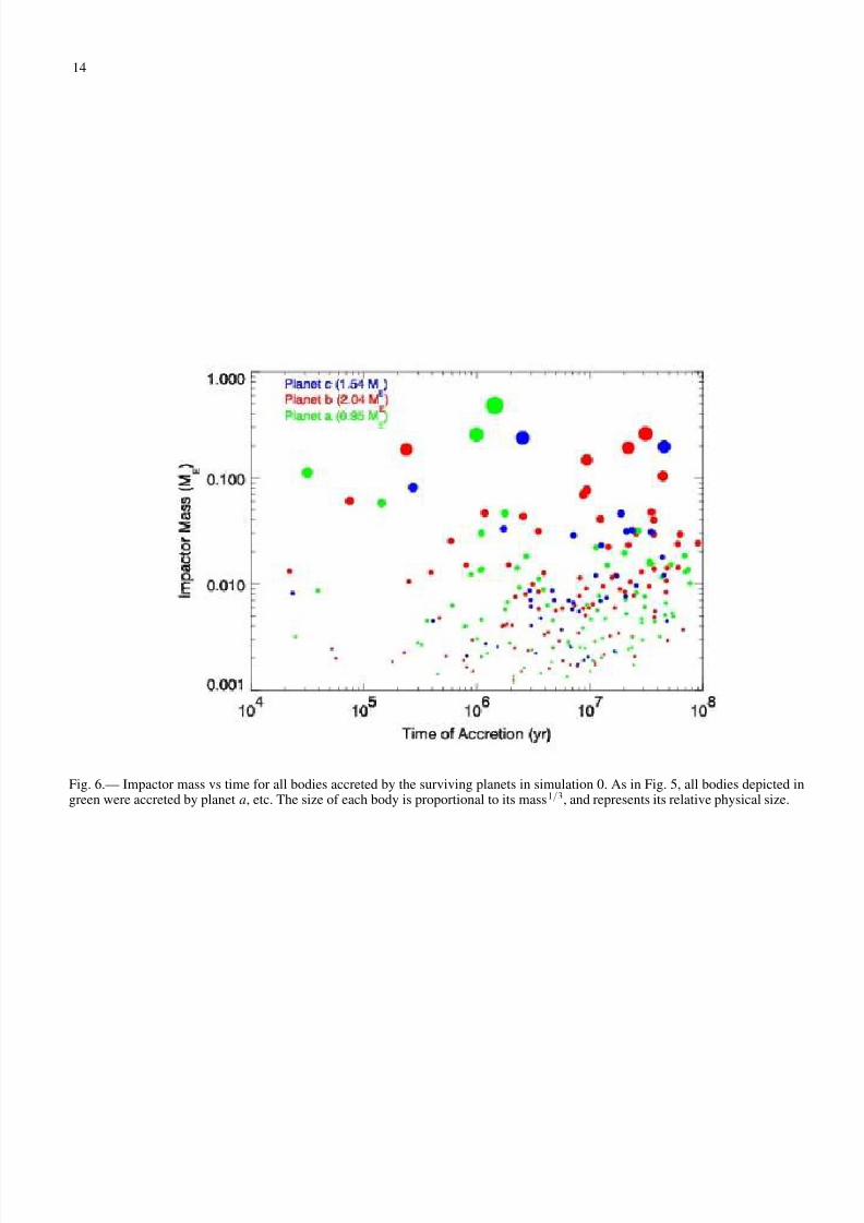
Figure 6 shows the mass of bodies accreted by each of thesurviving planets from simulation 0 as a function of time. Thesize of each body is proportional to its mass1/3, and thereforerepresents its relative physical size. Bodies of a range of sizes

are accreted by each planet throughout the simulation, althoughlarge impacts tend to happen later in the simulation. Some of these large impacts may form large satellites (moons). This isdiscussed in detail in Paper 2.

The radial time dependence of accretion seen in Fig. 5 is re-flected in the positions of ejected bodies. Figure 7 shows thestarting semimajor axes as a function of time of all bodies thatwere either ejected (blue) or accreted (red) by Jupiter. Thesebodies have had their eccentricities increased and had close en-counters with Jupiter, which has either devoured them or scat-tered them from the system. During the first part of the sim-ulation, only bodies past 4 AU are destroyed by Jupiter. Butafter∼ 107 years, the initial location of ejected bodies is a scat-



5

ter plot, signaling the end of the isolation of accretion zones.Bodies from throughout the terrestrial region are scattered intointerstellar space via close approaches to Jupiter.

In a disk of purely massless or non self-interacting particles,there would be no change in the trend like the one in Fig. 7at 107 years. Rather, through secular forcing, bodies from theouter asteroid belt would have close encounters with Jupiter andbe ejected. The zone cleared out by Jupiter would slowly widenin time, asymptotically reaching the point where the forced ec-centricity could not induce a close enough approach to Jupiter.Additional zones would be cleared out via mean motion res-onances. However, there would be no abrupt changes in thezones from which particles are ejected or accreted. This illus-trates an important effect of the self-gravity of the protoplane-tary disk.

4.2. Eccentricity Evolution

Previous simulations of terrestrial accretion have not suc-ceeded in reproducing the very low eccentricities of Earth,Mars, and Venus (Agnor et al. 1999; Chambers 2001; RQL04).The final eccentricities of the three planets at the end of the in-tegration are 0.03, 0.09, and 0.07 for planets a, b, and c, respec-tively. However, these are instantaneous values not necessarilyrepresentative of the long-term evolution of the system. Themean eccentricities for planets a, b, and c from 100-200 Myrare 0.048, 0.039, and 0.057.

Figure 8 shows the eccentricity evolution of each planet fromsimulation 0 through time. During the first 20 Myr, while theseplanets were accreting material at a very high rate, their ec-centricities remain relatively low, below 0.05-0.10. Collisionstend to circularize orbits, because they are most likely to happenwhen one body is at aphelion and the other at perihelion. In theperiod from 20-80 Myr, the planets’ eccentricities increase andfluctuate wildly due to numerous close encounters with othermassive bodies, which may increase eccentricities, but a slower

rate of collisions. After this time, the planets’ eccentricities aredamped through interactions with the remaining small bodiesin the system. The planets’ eccentricities reach very low valuesat t ∼ 150 Myr. The mean eccentricities of the three planetsfrom 150-170 Myr are 0.033 for planet a, 0.026 for planet b,and 0.057 for planet c.

At about 173 Myr, there is a jump in the eccentricities of the two inner planets, from about 0.03 to 0.05. This occurreddue to the scattering of a Moon-sized (0.02 M⊕) body fromthe asteroid belt into the inner terrestrial zone. Figure 9 showsthe semimajor axes vs time of all surviving bodies for the last50 Myr of the integration. Jupiter and the terrestrial planetsare labeled by their final masses. Several bodies are ejected be-tween 150-170 Myr, shown as verticalspikes as their semimajor

axes increase to infinity. Beginning at t ≈ 160 Myr, two bodiesin the asteroid belt begin to interact strongly and have severalclose encounters. At t = 173 Myr, the smaller, roughly lunar-mass body is scattered by the larger, Mars-sized body into theterrestrial region. Its eccentricity is large enough that over thenext twenty million years, this body has several close encoun-ters with all three of the terrestrial planets, causing a large jumpin their eccentricities. In time, the bodyis scattered outward andcollides with Jupiter at t = 193 Myr. Incidentally, the roughlyMars-mass scattering body is the largest object in the asteroidbelt at this time, but is ejected from the system at t = 198 Myr.

It is interesting to note in Fig. 8 how closely the eccentricityof the inner two planets track each other in time. Throughoutthe simulation, most sharp jumps are seen in the eccentricity

evolution of both bodies, and sometimes in the outer planet aswell. By examining the planets’ longitudes of perihelion, wehave determined that planets a and b are in a secular resonance.Figure 10 shows a histogram of the relative orientation of thetwo planets’ orbits. The relative orientation is measured by thequantityΛ, the difference in the two planets’ longitudes of per-ihelion, normalized to lie between 0 and 180 degrees (Barnes& Quinn 2004). The sharp spike seen at Λ

≈120◦ with the

tail to higher Λ values is the signature of secular resonance. Itindicates that the orbits of planets a and b are librating aboutanti-alignment, with an amplitude of about 60◦. The two plan-ets’ eccentricities are out of phase – planet a’s eccentricity islow when planet b’s is high, and vice versa. An interesting casefrom simulation 2a involving habitability will be discussed insection 8.

We explore two measures of the total dynamical excitementof the system as a function of time. The mass weighted eccen-tricity of all bodies is simply

MWE =

j m j e j

j m j

, (1)

where we sum over all surviving bodies j (excluding Jupiter).The angular momentum deficit measures the deviation of a setof orbits from perfect, coplanar circular orbits. This makes in-tuitive sense because the orbital angular momentum correlatesroughly with the perihelion distance, so a circular orbit has themaximum angular momentum for a given semimajor axis. Theangular momentum deficit includes both the inclination and ec-centricity of bodies in its formulation, and is defined by Laskar(1997) as

Sd =

j m j

√a j

1− cos(i j)

1− e2

j

j m j√

a j

, (2)

where, in this case, i j refers to a body’s inclination with respectto the plane of Jupiter.Figure 11 plots the mass-weighted eccentricity and angular

momentum deficit of all bodies through the course of the sim-ulation. The two measures of dynamical excitement track eachother fairly well through the simulation, although the angularmomentum deficit contains many more rapid fluctuations intime. This is because Sd is more sensitive than the MW E tosmall bodies, which may attain very high eccentricities and in-clinations through close encounters. Each spike in Sd is due toa single, high-eccentricity (or high-inclination) particle whichdoes not persist in this excited state. Rather, such a particlequickly falls into the Sun or is ejected from the system. Forexample, the four ejection events between 150-170 Myr seen in

Fig. 9 can be correlated with small spikes in the angular mo-mentum deficit in Fig. 11. Short term variations in the mass-weighted eccentricity are due to a combination of close encoun-ters which pump up eccentricities, and destruction of high-ebodies via ejections or collisions, which decreases the mean ec-centricity. In addition, both the mass weighted eccentricity andangular momentum deficit exhibit the jump at 173 Myr associ-ated with the close encounter shown in Fig 9.

The mass weighted eccentricity of the four terrestrial planetsin the Solar System and the largest asteroid, Ceres, is 0.037.The mean for the final 20 Myr of simulation 0 is 0.069, butfor the low eccentricity period between 150 and 170 Myr, itis 0.046. The terrestrial planets in this simulation have signif-icantly lower eccentricities than in most previous simulations



6

(e.g. Chambers 2001; RQL04). However, they are still largerthan those in the Solar System.

Using 3 million year average values from Quinn et al. (1991),the angular momentum deficit of the Solar System terrestrialplanets and Ceres is 0.0017, much smaller than Sd in Fig. 11.However, the value from simulation 0 is dominated by the fewsmall bodies that remain in the asteroid belt on relatively higheccentricity and inclination orbits. If we restrict ourselves toonly the three massive terrestrial planets, the value of Sd de-creases sharply to roughly 0.0037 for the last 20 Myr of thesimulation. In the period of very low eccentricities, from about150-170 Myr, Sd averaged 0.0026, only 50% higher than for therecent, time-averaged Solar System. If we include only the ter-restrial planets in the calculation, then Sd remains unchanged at0.0017. However, if we include only Venus, Earth, and Mars,Sd drops to 0.0013. This indicates that the planets in simulation0 are slightly more dynamically excited than the Solar System,but not by a large amount.

4.3. Evolution of the asteroid belt

The evolution of orbits in the asteroid belt, defined to be exte-rior to 2.2 AU (roughly the 4:1 resonance with Jupiter), differsfrom that in the terrestrial region, as no large bodies remainafter 200 Myr. The top panel of Figure 12 shows the most mas-sive body in the asteroid belt from simulation 0 through time.Bodies up to 0.26 M⊕ may exist in the asteroid belt. However,these bodies are not able to survive in this region, and are re-moved by scattering from either Jupiter or other asteroid beltbodies. Many embryo-sized bodies did not accrete in the aster-oid belt, but rather formed closer to the Sun and were scatteredoutward, where their eccentricities were damped causing themto remain on orbits in the asteroid belt. Accretion did take placein the asteroid region in simulation 0, but only to a limited ex-tent. Nine bodies originating in the region reached masses of 0.05 M⊕, and four reached 0.1 M⊕. The most massive locally-

formed body has 0.2 M⊕. Accretion was primarily confined tothe inner belt, as no bodies larger than 0.1 M⊕ formed past 3AU.

Many previous authors (e.g. Agnor et al. , 1999; Morbidelliet al. , 2000; Chambers 2001) assumed that all of the mass inthe asteroid belt was in the form of ≥Mars-sized planetary em-bryos. If these embryos form via oligarchic growth, separatedby 5-10 mutual Hill radii, these would have masses in the as-teroid belt between about 0.08 and 0.17 M⊕. By starting oursimulation from smaller bodies, we see that only a handful of such objects could actually form in the region on the relevanttimescales (although we have not included the effects of verysmall bodies, which may be significant – Goldreich et al. 2004).Our results suggest that initial conditions containing embryos

throughout the asteroid belt may not be realistic. This has im-portant implications for the water delivery process, and is dis-cussed in Paper 2.

The middle panel of Fig. 12 shows the evolution of the to-tal mass in the asteroid belt. Our initial conditions includedobjects out to 5 AU. Virtually all particles exterior to the 3:2Jupiter resonance at 4.2 AU were removed in the first few thou-sand years, causing the immediate steep drop from 4.9 M⊕ to4.2 M⊕ in the first 10 thousand years. After the initial drop,mass is continuously lost from the asteroid belt. Most objectsare either scattered into the terrestrial region to be incorporatedinto the terrestrial planets, or undergo a close encounter withJupiter and are ejected from the system. The total mass ejectedover the course of the simulation is 3.08 M⊕ out of 9.9 M⊕

of total solid mass. In addition, 0.66 M⊕ collided with Jupiter,and 0.02 M⊕ hit the Sun.

The asteroid belt is almost completely cleared of material,even though Jupiter is on a circular orbit. After 200 Myr, onlyfive bodies remain in the asteroid belt, four of which are clus-tered around 3.1 AU (see Fig. 2), corresponding to the outermain belt in our Solar System, which is dominated by C-typeasteroids. The total mass of these five surviving bodies in sim-ulation 0’s asteroid belt is 0.07 M⊕, roughly 1.5% of the totalmass. We continued the simulation to 1 Gyr, at which time onlyone 0.03 M⊕ body remained in the asteroid belt, comprisingonly 0.6% of the initial mass. Models of the primordial surfacedensity of the asteroid belt suggest that the asteroid belt in ourSolar System has been depleted by a factor of 102

− 103 (e.g.,Weidenschilling 1977). Our results imply that such clearing isa natural byproduct of the evolution of the disk. As suggestedby Morbidelli et al. (2000), the asteroid belt may be clearedsimply by self-scattering of bodies onto unstable orbits such asresonances with Jupiter. We show that this can occur even witha very calm dynamical environment, with Jupiter on a circularorbit. In this situation, Jupiter’s orbit does not precess (indeed,precession is meaningless with a circular orbit), so there areno secular resonances in the asteroid belt (such as the ν 6 res-onance with Saturn at 2.1 AU). Tsiganis et al. (2005) suggestthat the giant planets did not acquire appreciable eccentricitiesuntil about 600 Myr after the start of planet formation. Thus,even in this framework, the asteroid belt may have been rapidlycleared by the self-gravity of the disk.

The bottom panel of Fig. 12 shows the mass-weighted eccen-tricity through time of all bodies in the asteroid belt. A com-parison with Fig. 11 shows that bodies in the asteroid belt havesignificantly higher eccentricities than those in the inner terres-trial region throughout the simulation. This is simply becausebodies in the asteroid belt feel stronger perturbations than bod-ies closer to the Sun, due to Jupiter’s proximity. In other words,

the magnitude of the forced eccentricity for any particle in theasteroid belt is higher than for one in the terrestrial region. Intime, the amplitude of short term oscillations in the MWE in-creases as the number of bodies decreases.

5. SIMULATIONS 1A AND 1B: 1038 INITIAL PARTICLES

Simulations 1a and 1b both start with 38 planetary embryosto 2.5 AU, and 1000 0.006 M⊕ “planetesimals” between 2.5and 5 AU (see Fig. 1). The starting positions of all embryosand planetesimals are identical in simulations 1a and 1b. Theonly difference between the two simulations is how planetesi-mals are treated. In simulation 1a, planetesimals are massivebodies which interact gravitationally with all other bodies in

the simulation. In simulation 1b, however, planetesimals feelthe gravitational presence of the embryos and Jupiter, but noteach other’s presence. In addition, these non-interacting plan-etesimals may not collide with each other. Any differences inthe outcome of the two simulations therefore has to do with theproperties of these particles.

The reasons for running a simulation which includes nonself-interacting particles are several. Physically, we chose torun simulation 1b to test the importance of the self-gravityamong small bodies in the protoplanetary disk (included in sim-ulation 1a, but not in 1b). The effects are surprisingly impor-tant, as described below. In addition, the computational expenseof including test particles is much less than for self-interactingparticles, and scales with the number of particles N as N instead



7

of N 2. Therefore, many more such particles may be included ina simulation. However, the limitations of such simulations mustbe understood.

Figures 13 and 14 show six snapshots in the evolution of simulations 1a and 1b, respectively. One difference betweenthe two simulations that is immediately evident is the shapeof mean-motion resonances with Jupiter in the asteroid belt.In simulation 1a, the vertical structure of these resonances iswashed out within 1 Myr, as resonant planetesimals excitedby Jupiter excite other planetesimals in turn, and effectivelyspread out the resonance. In simulation 1b, however, the reso-nant structure is more confined and lasts longer, because of thelack of planetesimal-planetesimal encounters. The shape of the3:2 resonance with Jupiter in simulation 1b is still intact after 1Myr, and can be seen in Fig. 14. In both simulations, a swarmof surviving planetesimals appears to sweep into the terrestrialregion at between 10 and 30 Myr, damping the eccentricities of large bodies. These planetesimals also deliver water to the sur-viving planets. In time, the numbers of planetesimals dwindle,but at different rates for the two simulations. This has importanteffects on the final eccentricities of the surviving planets, and isdiscussed below.

There are several similarities in the final planetary systemsfrom simulations 1a and 1b. The positions of the two innerplanets in each simulation are comparable (see Table 2 for de-tails), although the masses of these planets differ significantly.The total mass in the three surviving planets from each simu-lation is nearly identical, 3.3 M⊕. The total water content of these planets is also similar, although the planets in simulation1a are slightly more water-rich, containing a total of 132 oceansof water as compared with 83 oceans contained in the planetsof simulation 1b.

There exist significant differences between simulations 1aand 1b. Figure 15 shows the growth of the surviving terrestrialplanets in simulations 1a (top panel) and 1b (bottompanel). It is

clear that planets form faster in simulation 1a – they reach a sig-nificant fraction of their final mass at shorter times. In addition,the final large accretion event for each planet in simulation 1aoccurs before t ≈ 60 Myr, while in simulation 1b this happensbetween roughly 70-90 Myr.

The main difference between the two simulations is the tim-ing of the destruction of particles. Gravitational self-scatteringof planetesimals in simulation 1a decreases the residence timeof these bodies in the asteroid region compared with simula-tion 1b, and scatters them onto unstable orbits. Eventually,these bodies either have a close encounter with Jupiter and areejected, or collide with a larger protoplanet. In addition, plan-etesimal collisions may occur, further decreasing the number of particles, although this effect is relatively minor.

The overall effects of this self-gravity are similar to those of the mass of asteroid region planetesimals explored in RQL04.In RQL04, we showed that more massive planetesimals causethe terrestrial planets to be more massive, more water-rich, toform more quickly, and to be fewer in number. Here we seethat the self-gravity of planetesimals accelerates planet forma-tion and moderately increases the water content of the terrestrialplanets. The final planets from simulations 1a and 1b both con-tain roughly the same amount of mass. We can apply this to ourresult from RQL04, that a larger planetesimal mass causes theformation of a smaller number of more massive planets. Thateffect must be due to the amount of mass in the asteroid regionin the “case (i)” simulations from RQL04, and not just dynam-

ical self-stirring.The top panel of Figure 16 shows the evolution of the num-

ber of surviving particles in simulations 1a (blue) and 1b (red).The number of planetesimals drops much more rapidly in sim-ulation 1a, and all are destroyed by t ≈ 140 Myr. The total massin each simulation that either collides with Jupiter or is ejectedis very similar, roughly 6 M⊕ of the 9.3 starting M⊕. Mostof this is in the form of planetesimals, although some embryosare ejected. The evolution of the embryos is similar for the twocases. This is not surprising as embryos reflect the evolution of the inner disk, which starts with no planetesimals.

The bottom panel of Fig. 16 shows the mass-weighted ec-centricity of all surviving particles from simulations 1a and 1bas a function of time. Eccentricities in both simulations growrapidly at the start. Simulation 1b reaches higher eccentricitiesin the heavy accretion phase before 50 Myr. This is becauseplanetesimals cannot damp their own eccentricities, which areelevated from a distance by secular and resonant perturbationsfrom the embryos and Jupiter. In simulation 1a, collisions anddynamical stirring among planetesimals damp these eccentric-ities. In time, the eccentricities of both systems decrease, andflatten off at similar levels, with mass-weighted eccentricities of 0.05-0.07. Eccentricities are barely damped at all in either sim-ulation after 100 Myr, as the number of total bodies has beenreduced to just a few.

We may have run into a resolution limit, as no planetesi-mals remain at the end of simulation 1a or 1b. The only refugeof such bodies is the asteroid region, separated from both theterrestrial planets and Jupiter. The dynamical effects of smallbodies on the planets are important in terms of damping eccen-tricities and inclinations. It is not clear from our simulationswhether the vast majority of small bodies are necessarily de-stroyed within 200 Myr, meaning that even higher-resolutionsimulations are useless. A more complex treatment of terres-trial accretion could generate additional particles during each

collision. This remains as an avenue for future study.It is clear from the 10 Myr and 30 Myr panels of Figs. 13and 14 that planetary embryos do exist in the asteroid region inboth simulations 1a and 1b, even though the planetesimals insimulation 1b cannot accrete. These embryos did not form insitu, but were fully formed at the start of the simulation, interiorto 2.5 AU, and were scattered into the asteroid belt in a pro-cess similar to “orbital repulsion” (Kokubo & Ida 1995). Theembryos’ eccentricities were increased by gravitational stirring,and they were scattered beyond 2.5 AU. Dynamical frictionacting on the large bodies damped their eccentricities withoutgreatly altering their semimajor axes, thereby moving them outinto the asteroid region. In this area, the orbits of embryos canbe stable on 100 Myr timescales. Indeed, in simulation 1a, one

embryo formed at 1.8 AU, quickly grew to 0.35 M⊕, and wasscattered into the asteroid region. It survived there for 200 Myruntil being ejected at 211 Myr.

Few embryos formed in the asteroid belt in simulation 1a.Although accretion in the asteroid region did occur, only ahandful of bodies accreted multiple other planetesimals, andonly five accumulations contained four or more planetesimals.Indeed, the largest accumulation contained 8 planetesimals to-taling only 0.05 M⊕, comparable in size to the smallest em-bryos in the inner part of the disk. Embryos in the 2-2.5 AUregion, separated by 5-10 mutual Hill radii, are typically 0.1-0.2 M⊕. So, even the largest planetesimal accumulation wasa factor of 2-3 smaller than its isolation mass. No large em-



8

bryos formed in the asteroid belt in simulation 1a, although afew embryos did form in the asteroid region in simulation 0,as discussed above. We conclude that accretion can happen inthe asteroid belt, but only to a limited degree, forming a smallernumber of less massive embryos than assumed in most previousaccretion simulations (e.g. Morbidelli et al. , 2000).

6. SIMULATIONS 2A AND 2B: 1054 INITIAL PARTICLES

In simulations 1a and 1b we assumed that embryos formedonly out to 2.5 AU, but in simulations 2a and 2b we assumethat they formed all the way out to 5 AU. This corresponds toeither a fast growth of embryos, as advocated by Goldreich et al. (2004), or perhaps a very slow growth of Jupiter. Simula-tions 2a and 2b have identical starting conditions (see Fig. 1),with 54 planetary embryos throughout the terrestrial region,embedded in a disk of 1000 “planetesimals” of 0.003 M⊕ each.Roughly two thirds of the mass is in the form of embryos, andone third in planetesimals. The only difference between sim-ulations 2a and 2b is the way in which the planetesimals aretreated: in simulation 2b the planetesimals do not feel eachother’s presence, but in simulation 2a all particles are fully self-interacting.

Interestingly, the initial conditions for simulations 1a and 1bare reasonable if embryos form via the Goldreich et al. (2004)model, but are unrealistic if they follow the results of Kokubo& Ida (2000, 2002). The oligarchic growth phase is thoughtto end when the total mass in planetesimals and embryos iscomparable (e.g., Lissauer 1993). Our initial conditions there-fore represent a time after the completion of oligarchic growth.However, Kokubo & Ida’s model of oligarchic growth suggeststhat there may not be enough time for embryos to form in theouter terrestrial zone, in the asteroid region beyond 2-2.5 AU.Indeed, analysis of simulations 0 and 1a suggests that, if Jupiterwas fully formed before embryos formed in the asteroid region,

then perhaps five to ten embryos could have formed in this re-gion. These would be sub-isolation mass objects, with massesof ∼ 0.05 M⊕ rather than the 0.1−0.2 M⊕ embryos in Fig. 1. InKokubo & Ida (2000)’s model, embryos at 2.5 AU take roughly10 Myr to form. The lifetime of gaseous disks around otherstars is ≤ 10 Myr (Briceño et al. 2001), constraining the for-mation time of gas giant planets. Embryos form more slowly atlarger orbital radii, so this model predicts that oligarchic growthin the asteroid region must have occurred in the presence of thegiant planet, stunting the formation of embryos.

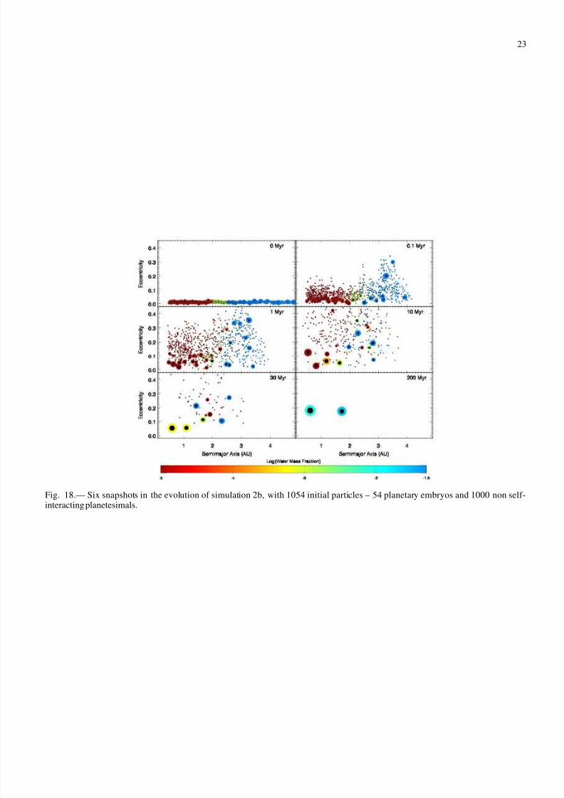
Figures 17 and 18 show snapshots in time of simulations 2aand 2b, respectively. The evolution of the two simulations isqualitatively similar in the first few Myr, but the outcomes aredrastically different. Simulation 2a forms four terrestrial plan-

ets, including two in the habitable zone. Simulation 2b, in con-trast, forms only two planets, one interior to and one exterior tothe habitable zone.

Interactions among planetesimals appear to be very impor-tant to the dynamics of the system. The outcome of simulation2b is very surprising in that the final terrestrial planets have veryhigh eccentricities (e∼ 0.2), not expected for a >1000 particlesimulation. Eccentricities in simulation 2a are slightly higherthan in simulations 0, 1a and 1b, but are only about half of those in simulation 2b (e ∼ 0.1). The final angular momentumdeficit of the planets in simulation 2a is one third of that forsimulation 2b.

The early evolution of the simulations is not surprising –bodies are excited by resonances and mutual encounters. The

shapes of resonances are quickly washed out by the interactionsamong embryos. Dynamical friction between the embryos andplanetesimals damps the eccentricities of the embryos and in-creases that of the planetesimals. This process appears to bestronger in simulation 2a than in simulation 2b. In each of thefinal three panels of Figs. 17 and 18, large bodies in simulation2a have significantly smaller eccentricities than those in sim-ulation 2b. The feeding zone of each planet is affected by itseccentricity; a larger eccentricity implies a larger radial varia-tion during a body’s orbit, causing it to intercept more materialthan for a circular orbit (Levison & Agnor 2003). Indeed, thefinal planets in simulation 2b have high eccentricities and largemasses.

Figures 19 and 20 show the time evolution of several aspectsof simulations 2a and 2b, respectively. The top panels show thegrowth of the two final planets. The middle panels show thenumber of surviving bodies, both embryos and planetesimals,through time. The bottom panels show the mass-weighted ec-centricity of all surviving bodies as a function of time. Notethat the scale of the y axis for the bottom panels is different inthe two figures.

The formation timescales are similar in simulations 2a and2b. In both cases most accretion takes place in the first 30 Myr.The planets reach a significant fraction of their final masses bythe end of rapid accretion. After this time, the planets accrete(often water-rich) planetesimals as well as possibly undergoinga large impact with another embryo.

In both simulations, the evolution of the mass-weighted ec-centricity begins with the same rapid increase and bumpy pro-file seen in simulation 0 (Fig. 11). The eccentricities in sim-ulation 1a in this early stage are slightly lower than those insimulation 2b. Eccentricities decrease in both simulations aftert ≈ 40 Myr, after which their evolutions diverge. In both simu-lations, the decrease is followed by a sharp increase. However,the magnitude and duration of the increase are drastically dif-

ferent. In simulation 1a, the mass-weighted eccentricity reaches0.2 at t = 50 Myr, then begins a slow decline for the rest of thesimulation. In simulation 2b, the eccentricity reaches values of almost 0.4 at t ≈ 60 Myr, and does not flatten out until 100 Myr.When it does flatten out, it does so at a much higher level thanin the other simulations, about 0.2. The middle panel of Fig 20shows that the increase in eccentricity at 50 Myr correspondsto the time when only a very few large bodies remain in thesystem, at the end of the rapid accretion phase. Indeed, onlyfour embryo-sized bodies survive to t = 45 Myr. As seen in theupper panel of Fig 20, two of these bodies are accreted by thesurviving planets at 76 Myr and 127 Myr. However, the num-ber of embryos at this time in simulation 2a is comparable. Thedifferences lie in the evolution of the planetesimals.

During the time of very high eccentricities in simulation 2b,between roughly 50 and 100 Myr, only a few large bodies re-main. Less than 100 planetesimals remain at the beginning of this period, and their destruction rate is accelerated at t ∼ 50Myr, such that all are ejected by t ≈ 75 Myr. The increase ineccentricities is due to the lack of dissipative forces, i.e. nosmall bodies remain to provide dynamical friction. The sameacceleration in the destruction rate of planetesimals is seen insimulation 1a at t ∼ 55 Myr. However, the curve flattens out,and several tens of planetesimals remain after the sharp increasein eccentricities at 50 Myr. Thus, large bodies in simulation 1acontinue to feel dynamical friction, while those in simulation1b do not.



9

Why do self-interacting planetesimals provide more dissipa-tion than non self-interacting ones? In simulation 2a, eccentric-ities reached by the planetesimals are much smaller than in sim-ulation 2b. This implies that interactions among planetesimalsdamp their eccentricities, i.e. planetesimals can feel dynami-cal friction from other planetesimals. By damping planetesi-mals’ excitations, more are on low-inclination orbits likely tobe encountered by embryos, increasing the damping. In addi-tion, by staying on lower-excitation orbits, the lifetime of self-interacting planetesimals is longer. Unfortunately, the compu-tational time needed to integrate the orbits of N self-interactingbodies scales as N 2, while non self-interacting bodies only scaleas N .

It is interesting that self-interacting planetesimals survivelonger in simulation 2a than simulation 2b, but non self-interacting planetesimals survive longer in simulation 1b thansimulation 1a. In simulations 1a, planetesimals are primarilydestroyed by ejection after being scattered by other planetesi-mals onto unstable resonances with Jupiter in the asteroid re-gion. Non self-interacting particles in unstable resonances arecleared out quickly, but nearby orbits are not perturbed into in-stability. In contrast, the main destruction mechanism of plan-etesimals in simulations 2a and 2b is scattering by embryos ontounstable orbits. The eccentricities of non self-interacting plan-etesimals increase more rapidly than self-interacting planetesi-mals, so they are destroyed more quickly.

When all the planetesimals are destroyed, simulations pro-ceed in the same fashion as previous, low resolution simula-tions which formed planets with relatively large eccentricities(e.g. Chambers 2001; RQL04). Secular perturbations and closeencounters among the few remaining bodies excite their eccen-tricities. The feeding zones of these eccentric embryos are en-larged, and bodies are accreted until the system stabilizes with asmall number of relatively massive, eccentric terrestrial planets.This occurs in simulation 2b, as planetesimals are destroyed

before the end of accretion. In simulation 2a, however, someplanetesimals survive through the end of accretion, keeping ec-centricities low and planetary feeding zones narrow. The sur-viving planets in simulations 2a and 2b reflect this importantdifference in the evolution of their planetesimal populations.

A problem with our simulations is that the number of parti-cles can only decrease. Realistic collisions between large bod-ies create a swarm of debris, the details of which depend on thecollision velocity and angle (Agnor & Asphaug, 2004). Inter-actions between large bodies and this collisional debris tendsto circularize the orbits of large bodies via dynamical friction(Goldreich et al. 2004). The reason for the high eccentricitiesin simulation 2b is the rapid destruction of all the small bod-ies. We included enough planetesimals to “resolve” the early

parts of the simulation, but the planetesimals were all destroyedquickly. This problem may be solved in two ways, by eitherstarting the simulation with even more particles than includedhere, by using self-interacting planetesimals (as in simulation2a), or by creating debris particles during collisions. It wouldbe very interesting to self-consistently create debris particlesduring oblique or high-velocity collisions, but this is left to fu-ture work.

7. CONCLUSIONS

We have run five simulations of terrestrial accretion with un-precedented resolution. The planets that formed were qualita-tively similar to those formed in previous simulations, such as

RQL04. The mean eccentricities of our planets are smaller thanin previous simulations, averaging about 0.05 vs. 0.1, but theyremain larger than those of Venus, Earth, and Mars. This maybe due to the resolution of our simulations, as the number of small bodies dwindles at late times. Perhaps a higher resolu-tion simulation will further damp the terrestrial planet eccen-tricities. Future simulations may also include additional dissi-pative effects, such as accounting for dynamical friction fromcollisional debris.

We have uncovered several significant, previously unrecog-nized aspects of the accretion process:

1. The feeding zones of the terrestrial planets widen andmove outward in time, as shown in Fig. 5. While themass in a given annulus is dominated by small bodies,the damping effects effectively isolate that region by sup-pressing eccentricity growth. In time, large bodies formand material is scattered out of the region, ending its iso-lation period. The isolation time corresponds roughly tothe oligarchic growth phase, and proceeds rapidly in theinner disk and moves outward in time. Assuming thatembryos form slowly (as in Kokubo & Ida 2000), planets

do not accrete water-rich material until at least 10 Myrafter the start of a simulation, at which time most planetsare a sizable fraction of their final mass.

2. The growth of planetary embryos in the asteroid belt mayhave been stunted by the presence of a giant planet. If embryos formed relatively slowly, following the resultsof Kokubo & Ida (2000), then perhaps ten or so smallish,∼ 0.05 M⊕ embryos could form in the inner belt, out toabout 3-3.5 AU. Beyond this, Jupiter’s gravitational ef-fects, as well as intrusion from embryos formed closer tothe Sun, prevented their accretion. This result is indepen-dent of Jupiter’s time of formation, because the 10 Myrtimescale for embryos to form out to 2.5 AU (Kokubo &

Ida 2000) corresponds to the upper limit on the formationtime of Jupiter (Briceño et al 2001). Embryos can forminterior to 2.5 AU, be scattered into the asteroid belt andreside there for long periods of time, but are unlikely toform in situ. However, this result is model-dependent:Goldreich et al. (2004) calculate much shorter embryoformation timescales. In their model, embryos wouldcertainly have formed before the giant planets, assumingthese to form via core-accretion (Pollack et al. 1996) on atimescale of millions of years. The speed of embryo for-mation has important implications for the robustness of water delivery: if embryos form quickly, then the numberof bodies involved in water delivery is relatively small,and the process is relatively stochastic (although less than

in previous models – Morbidelli et al. 2004, RQL04).

3. Dynamical friction is a significant phenomenon for thegrowth of terrestrial planets. Indeed, even mall bod-ies feel dynamical friction from a swarm of other smallbodies. The high computational cost of fully-interactingsimulations is therefore necessary to ensure a realisticoutcome. The dynamics and outcome of simulations inwhich all particles interacted with each other were differ-ent than simulations in which our “planetesimals” werenot self-interacting. Most severe was the case of simula-tions 2a and 2b. In simulation 2a, more planets formedthan in simulation 2b (4 planets vs. 2) and the eccen-tricities of the final planets were far lower (e ≈ 0.1 vs.



10

e ≈ 0.2). The lifetime of planetesimals was much longerin simulation 2a, because of dynamical friction due othersmall bodies. The consequences of are important: thefraction of water delivered to terrestrial planets in theform of small bodies was twice as high in simulation 2a,and the timing of the delivery of water-rich embryos andplanetesimals also varied among the two simulations.

4. The asteroid belt is cleared of >99% of its mass as a nat-ural result of terrestrial accretion. Embryos and planetes-imals scatter each other onto unstable orbits such as meanmotion resonances with Jupiter. In time these bodies are

removed via ejections, or by colliding with bodies closerto the Sun. After ∼ 1 billion years, none of our simula-tions had more than 0.4% of their initial mass remainingin the asteroid belt. This result was also shown by Mor-bidelli et al. (2000) in the context of the current orbits of Jupiter and Saturn. In that case, many resonances exist inthe asteroid belt, including the important ν 6 secular res-onance with Saturn at 2.1 AU. Here we have shown thatthe asteroid belt is cleared even in a much calmer dynam-ical environment, with only one giant planet on a circularorbit.

REFERENCES

Agnor, C. B., Canup, R. M., & Levison, H. F. 1999. On the Character and Con-sequences of Large Impacts in the Late Stage of Terrestrial Planet Formation.Icarus, 142, 219.

Agnor, C., & Asphaug, E. 2004. Accretion Efficiency during Planetary Colli-sions. ApJ, 613, L157.

Barnes, R. & Quinn, T., 2004. The (In)stability of Planetary Systems. ApJ 611,494-516.

Briceño, C., Vivas, A. K., Calvet, N., Hartmann, L., Pacheco, R., Herrera, D.,Romero, L., Berlind, P., Sanchez, G., Snyder, J. A., Andrews, P., 2001. TheCIDA-QUEST Large-Scale Survey of Orion OB1: Evidence for Rapid Disk Dissipation in a Dispersed Stellar Population. Science 291, 93-97.

Canup, Robin M., Asphaug, Erik 2001. Origin of the Moon in a giant impactnear the end of the Earth’s formation. Nature, 412, 708-712.

Chambers, J. E., 1999. A Hybrid Symplectic Integrator that Permits Close En-counters between Massive Bodies. MNRAS, 304, 793-799.

Chambers, J. E. 2001. Making More Terrestrial Planets. Icarus, 152, 205-224.Chambers, J. E. & Cassen, P., 2002. The effects of nebula surface density pro-

file and giant-planet eccentricities on planetary accretion in the inner Solarsystem. Meteoritics and Planetary Science, 37, 1523-1540.

Cyr, K. E., Sears, W. D., & Lunine, J. I. 1998. Distribution and Evolution of Water Ice in the Solar Nebula: Implications for Solar System Body Forma-tion. Icarus, 135, 537

Drake, M. J. and Righter, K., 2002. What is the Earth made of? Nature 416,39-44.

Goldreich, P., Lithwick, Y., & Sari, R. 2004. Final Stages of Planet Formation.ApJ, 614, 497

Gomes, R., Levison, H. F., Tsiganis, K., & Morbidelli, A. 2005. Origin of the cataclysmic Late Heavy Bombardment period of the terrestrial planets.Nature, 435, 466

Hayashi, C. 1981. Structure of the solar nebula, growth and decay of magneticfields and effects of magnetic and turbulent viscosities on the nebula. Prog.Theor. Phys. Suppl., 70, 35-53.

Hester, J. J., Desch, S. J., Healy, K. R., & Leshin, L. A. 2004. The Cradle of the Solar System. Science, 304, 1116

Kasting, J. F., Whitmire, D. P., and Reynolds, R. T., 1993. Habitable zonesaround main sequence stars. Icarus 101, 108-128.

Kleine, T., Munker, C., Mezger, K., Palme, H., 2002. Rapid accretion and earlycore formation on asteroids and the terrestrial planets from Hf-W chronom-etry. Nature 418, 952-955.

Kokubo, E., & Ida, S. 1995. Orbital evolution of protoplanets embedded in aswarm of planetesimals. Icarus, 114, 247

Kokubo, E. & Ida, S., 2000. Formation of Protoplanets from Planetesimals inthe Solar Nebula. Icarus 143, 15-27.

Kokubo, E. & Ida, S., 2002. Formation of Protoplanet Systems and Diversityof Planetary Systems. ApJ 581, 666.

Kornet, K., Rózyczka, M., & Stepinski, T. F. 2004. An alternative look at thesnowline in protoplanetary disks. A&A, 417, 151

Laskar, J. 1997. Large scale chaos and the spacing of the inner planets. A&A,

317, L75

Levison, H. F. & Agnor, C., 2003. The Role of Giant Planets in TerrestrialPlanet Formation. AJ, 125, 2692-2713.

Lissauer, J. J. 1993. Planet Formation. ARAA, 31, 129.Lissauer, J. J. 1999. How common are habitable planets? Nature 402, C11-

C14.Lodders, K., & Fegley, B. 1998, The planetary scientist’s companion. Oxford

University Press, 1998.Morbidelli, A., Chambers, J., Lunine, J. I., Petit, J. M., Robert, F., Valsecchi,

G. B., and Cyr, K. E., 2000. Source regions and timescales for the deliveryof water on Earth. Meteoritics and Planetary Science 35, 1309-1320.

Pollack, J. B., Hubickyj, O., Bodenheimer, P., Lissauer, J. J., Podolak, M., &Greenzweig, Y., 1996. Formation of the Giant Planets by Concurrent Accre-tion of Solids and Gas. Icarus, 124, 62-85.

Quinn, Thomas R., Tremaine, Scott, & Duncan, Martin, 1991. A three millionyear integration of the earth’s orbit. AJ 101, 2287-2305.

Raymond, S. N., Quinn, T., & Lunine, J. I., 2004. (RQL04) Making otherearths: dynamical simulations of terrestrial planet formation and water de-livery. Icarus, 168, 1-17.

Raymond, S. N., Quinn, T., & Lunine, J. I. 2005a. The formation and habit-ability of terrestrial planets in the presence of close-in giant planets. Icarus,177, 256-263.

Raymond, S. N., Quinn, T., & Lunine, J. I. 2005b. Terrestrial Planet Formationin Disks with Varying Surface Density Profiles. ApJ, 632, 670-676.

Raymond, S. N., Quinn, T., & Lunine, J. I. 2006. (Paper 2) High-resolutionsimulations of the final assembly of Earth-like planets 2: water delivery andplanetary habitability. Astrobiology, submitted, astro-ph/

Regenauer-Lieb, K., Yuen, D. A., & Branlund, J. 2001. The initiation of sub-duction: Criticality by addition of water? Science 294(5542): 578-580.

Sasselov, D. D. & Lecar, M. 2000. On the Snow Line in Dusty ProtoplanetaryDisks. ApJ, 528, 995

Stevenson, D.J. & Lunine, J.I., 1988. Rapid formation of Jupiter by diffusiveredistribution of water vapor in the solar nebula. Icarus 75, 146-155.

Stadel, Joachim Gerhard 2001. Cosmological N-body simulations and theiranalysis. PhD Dissertation, University of Washington, Seattle.

Tsiganis, K., Gomes, R., Morbidelli, A., & Levison, H. F. 2005. Origin of theorbital architecture of the giant planets of the Solar System. Nature, 435, 459

Weidenschilling, S. J. 1977. The distribution of mass in the planetary systemand solar nebula. Ap&SS, 51, 153

Wetherill, G. W., 1996. The Formation and Habitability of Extra-Solar Planets.Icarus, 119, 219-238.

Williams, D. M., Kasting, J. F., & Wade, R. A. 1997. Habitable moons aroundextrasolar giant planets. Nature, 385, 234-236.

Williams, D. M., & Pollard, D. 2002. Extraordinary climates of Earth-likeplanets: three-dimensional climate simulations at extreme obliquity. Inter-national Journal of Astrobiology, 1, 1

Yin, Qingzhu, Jacobsen, S. B., Yamashita, K., Blichert-Toft, J., Telouk, P.,Albarede, F., 2002. A short timescale for terrestrial planet formation fromHf-W chronometry of meteorites. Nature 418, 949-952.



11

Fig. 1.— Our three sets of initial conditions for high-resolution simulations. The large circles at 5.5 and 5.2 AU are Jupiter-massgiant planets. The horizontal lines in simulations 1 and 2 represent 1000 planetesimals, which are distributed with orbital radius r asr −1/2, corresponding to the annular mass in a disk with an r −3/2 surface density profile.



12

Fig. 2.— Six snapshots in time from simulation 0, with 1885 initial particles. The size of each body corresponds to its relativephysical size (i.e. its mass M 1/3), but is not to scale on the x axis. The color of each particle represents its water content, and the dark inner circle represents the relative size of its iron core. There is a Jupiter-mass planet at 5.5 AU on a circular orbit (not shown).

Fig. 3.— The feeding zones of the three surviving massive planets from simulation 0 (see Table 2). The y axis represent the fractionof each planet’s final mass that started the simulation in a given 0.45 AU wide bin. The final configuration of the planets is shownat top of the figure (as in the 200 Myr panel from Fig. 2). The color of each curve refers to the horizontal colored line below eachplanet.



13

Fig. 4.— Mass vs time for the three surviving planets from simulation 0.

Fig. 5.— The timing of accretion of bodies from different initial locations for simulation 0. All bodies depicted in green wereaccreted by planet a, all blue bodies were accreted by planet b, and all red bodies were accreted by planet c. The relative size of eachcircle indicates its actual relative size. Impactors which had accreted other bodies are given their mass-weighted starting positions.



14

Fig. 6.— Impactor mass vs time for all bodies accreted by the surviving planets in simulation 0. As in Fig. 5, all bodies depicted ingreen were accreted by planet a, etc. The size of each body is proportional to its mass1/3, and represents its relative physical size.



15

Fig. 7.— The timing of the ejection and accretion by Jupiter of bodies from different starting locations. Note the change in the“ejection zone” at t ≈ 10 Myr .



16

Fig. 8.— Eccentricity vs time for the three surviving massive planets. See Table 2 for details.



17

Fig. 9.— Semimajor axes of all bodies from simulation 0 for the time period from 150-200 Myr. The three surviving terrestrialplanets and Jupiter are in bold and are labeled. Vertical spikes indicate a particle’s ejection from the system. Notice the encounterbetween a stray body and the terrestrial planets from about 173 to 193 Myr, which had a large effect on the eccentricities of thesurviving planets (see Fig. 8). The body’s eccentricity was large enough (> 0.4) that its orbit crossed that of planet a.

Fig. 10.— Normalized histogram of the relative orientation of the orbits of planets a and b from simulation 0 over one billion years.Λ represents the difference in the two planets’ longitudes of perihelion, normalized to lie between 0 and 180 degrees (Barnes &Quinn 2004). The spike at Λ ≈ 120◦ and tail to higher Λ values is reminiscent of a harmonic oscillator. It indicates that the twoplanets are locked in secular resonance, librating about anti-alignment with an amplitude of about 60 degrees.



18

Fig. 11.— Top panel – Mass weighted eccentricity vs time for all bodies from simulation 0, excluding Jupiter. Bottom Panel –Angular momentum deficit vs time for all bodies from simulation 0, also excluding Jupiter. These quantities are defined in Eqs. 1and 2.



19

Fig. 12.— Evolution of the asteroid belt (defined as 2.2 < a < 5.2 AU) in time for simulation 0. Top – the most massive body in theasteroid belt through time. Middle – total mass in the asteroid belt as a function of time. Bottom – Mass-weighted eccentricity of allbodies in the asteroid belt over time.



20

Fig. 13.— Six snapshots in the evolution of simulation 1a, with 1038 initial particles, all self-interacting.

Fig. 14.— Six snapshots in the evolution of simulation 1b, with 1038 initial particles – 38 planetary embryos and 1000 non self-interacting planetesimals.



21

Fig. 15.— The masses of all surviving bodies from simulations 1a (top panel) and 1b (bottom panel) as a function of time. Theinnermost planet in each case (planet a) is shown in green, the middle planet (planet b) in blue, and the outer planet (planet c) in red.



22

Fig. 16.— A comparison of the evolution of physical properties of simulations 1a (shown in blue) and 1b (red). Top: The number of surviving bodies, both planetesimals and planetary embryos. Bottom: The mass-weighted eccentricity of all surviving bodies.

Fig. 17.— Six snapshots in the evolution of simulation 2a, with 1054 initial particles, all self-interacting.



23

Fig. 18.— Six snapshots in the evolution of simulation 2b, with 1054 initial particles – 54 planetary embryos and 1000 non self-interacting planetesimals.



24

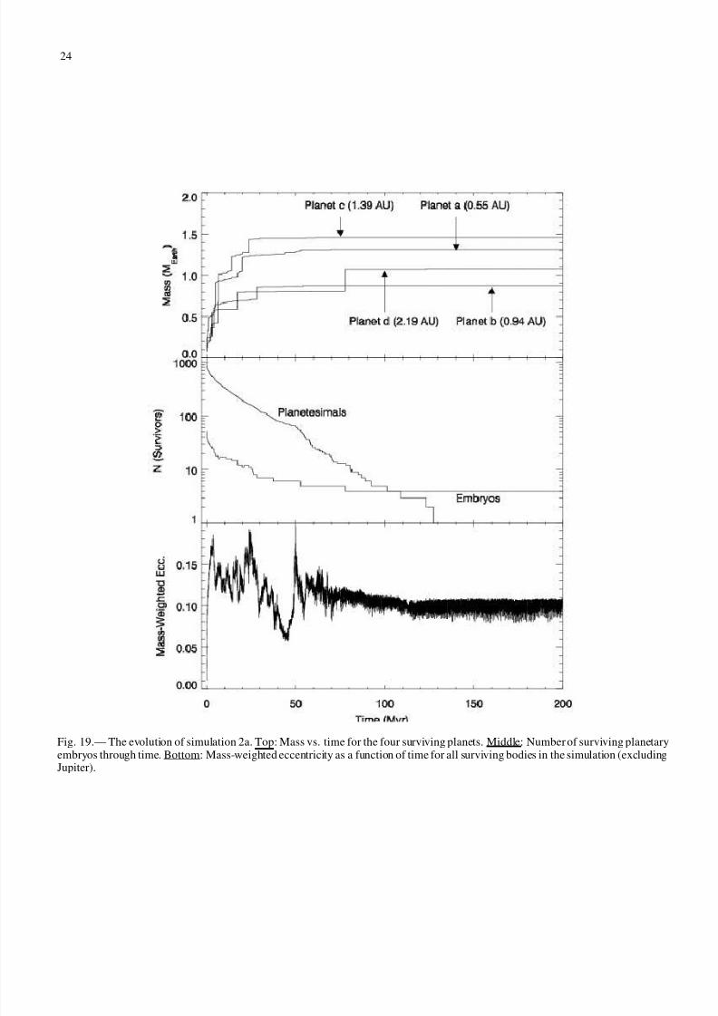
Fig. 19.— The evolution of simulation 2a. Top: Mass vs. time for the four surviving planets. Middle: Number of surviving planetaryembryos through time. Bottom: Mass-weighted eccentricity as a function of time for all surviving bodies in the simulation (excludingJupiter).



25

Fig. 20.— The evolution of simulation 2b. Top: Mass vs. time for the two surviving planets. Middle: Number of surviving planetaryembryos through time. Bottom: Mass-weighted eccentricity as a function of time for all surviving bodies in the simulation (excludingJupiter).

Documents

High-resolution simulations of the final assembly of Earth-like planets 1