HIGH-RESOLUTION FINITE VOLUME METHODS FOR DUSTY …faculty.washington.edu/rjl/pubs/dustyjet/sisc063501.pdfHIGH-RESOLUTION FINITE VOLUME METHODS FOR DUSTY GAS JETS AND PLUMES MARICA

HIGH-RESOLUTION FINITE VOLUME METHODS FOR DUSTY GAS JETS ANDPLUMES∗

MARICA PELANTI† AND RANDALL J. LEVEQUE‡

Abstract. We consider a model for dusty gas flow that consists of the compressible Euler equations for the gascoupled to a similar (but pressureless) system of equations for the mass, momentum, and energy of the dust. These setsof equations are coupled via drag terms and heat transfer. A high-resolution wave-propagation algorithm is used to solvethe equations numerically. The one-dimensional algorithm is shown to give agreement with a shock tube test problemin the literature. The two-dimensional algorithm has been applied to model expolsive volcanic eruptions in which anaxisymmetric jet of hot dusty gas is injected into the atmosphere and the expected behavior is observed at two differentvent velocities. The methodology described here, with extensions to three dimensions and adaptive mesh refinement, isbeing used for more detailed studies of volcanic jet processes.

Key words. Finite volume methods, high-resolution methods, volcanic flows, dusty gas, plumes, jets, shocks

AMS subject classifications. 65M06, 76T15

1. Introduction. We study compressible gas dynamics coupled with a suspended particulatephase having small volume fraction but possibly large density per unit volume relative to the gas. Werefer to the particulate phase as “dust” (though in some contexts it could represent liquid droplets) andthe mixture as a “dusty gas”. Dusty gas flows arise in many applications, from industrial processes togeophysical flows. One particular application, which was the original motivation for our work, is thestudy of volcanic ash plumes and pyroclastic flows. The numerical approach developed and tested hereshould be directly applicable in other contexts as well.

We ignore viscosity in the present work and use the compressible Euler equations to model theconservation of mass, momentum, and energy in the gas phase, using an ideal gas equation of state. Theparticulate phase is modeled by a similar system of equations for the conservation of mass, momentum,and energy of the dust. We ignore inter-particle collisions and assume there is no pressure componentin the momentum equations, using the so-called “pressureless dust” or “sticky particle” equations forthis flow (see Section 2). These two sets of conservation laws are coupled together through source termsthat model drag and heat transfer between the phases.

In the absence of coupling terms, we would have two decoupled sets of hyperbolic conservation laws.The pressureless dust equations are nonstrictly hyperbolic (since the sound speed is zero in the absenceof pressure) and have a degenerate structure in which delta shocks can arise, shocks at which deltafunction singularities form in this mathematical idealization. The source term coupling smooths outsingularities in the solution. The speed of sound in the dusty gas is lower than the sound speed of thepure gas phase, and can be substantially lower at high dust densities if there is sufficient coupling, i.e.,if the relaxation times of the momentum and heat transfer processes are sufficiently fast (see Section2.2). One effect of this is that dusty gas jets can be supersonic at relatively low velocities, and so theshock wave structures typically seen in supersonic jets are often observed at lower velocities than mightbe expected. In particular, jets of ash in volcanic eruptions can exhibit such structures, see e.g. [20].

The effect of gravity on both the gas and dust phase can also be included in the model when needed,as for example in the case of volcanic plumes where gravity plays a substantial role. One question ofparticular interest in this context is whether an eruption column rises high into the atmosphere as a“Plinian column” and slowly disperses downwind, or whether the column collapses with the heavierdust phase flowing along the surface. This depends on the balance between the downward force ofgravity and the upward momentum and buoyancy of the hot dense jet.

∗This work was supported in part by DOE grant DE-FG03-96ER25292 and NSF grant DMS-9803442. To appear inSIAM J. Sci. Comput. Version of February, 2006.

† Department of Applied Mathematics, University of Washington, Box 352420, Seattle, WA [email protected]

‡ Department of Applied Mathematics and Department of Mathematics, University of Washington, Box 352420, Seattle,WA 98195-2420. [email protected]

1

2 M. PELANTI AND R. J. LEVEQUE

Applications to volcanic jets will be explored in more detail in a forthcoming paper [37], in whichnumerical results obtained with our approach will be compared with results from a similar model anddifferent numerical method developed in the work of Neri, Esposti Ongaro, and co-workers [32, 34].Here we present the details of our numerical algorithm and several test problems.

The model is presented in more detail in Section 2 and the numerical algorithm is developed inSection 3. We use the wave-propagation algorithm as implemented in the clawpack software [24].This is a high-resolution finite volume algorithm for the hyperbolic conservation law portion of theequations, based on solving Riemann problems at each cell interface at every time step. The “f-waveformulation” [2], [27] of the algorithm is used in which the flux difference between neighboring cells isdecomposed into waves that are then used to update the cell averages in each cell. This formulationis preferable for the pressureless dust portion of the hyperbolic system, where we use the algorithmdeveloped in [28]. This formulation also allows us to incorporate the source term due to gravity in thegas dynamics portion of the hyperbolic system into the Riemann solver in such a way that hydrostaticbalance in the atmosphere is well maintained in the absence of flow or dust (with the pressure gradientbalancing the gravitational force on the gas). This is discussed in more detail in Section 6, where gravityis introduced. The gravitational force in the dust equations and the source terms modeling inter-phasedrag and heat transfer are all handled by a fractional step procedure, as described in Section 5.

Our goal is to keep the physical model as simple as possible while still allowing simulation of somefundamental features of hot dilute dusty flows in the presence of gravity. In particular, we ignoreviscosity within the gas phase and effects of turbulence. In modeling the structure of dusty gas jets asconsidered here this is a reasonable approximation.

Ultimately we hope that this approach will also be useful for modeling some aspects of volcaniceruptions in three dimensions over large domains to better understand hazards associated with activevolcanos. For this it is desirable to have a simple model that is applicable on mapped grids that followrealistic terrain and to which adaptive mesh refinement can also be applied. The present model hasbeen implemented on quadrilateral and hexahedral grids and adaptive mesh refinement has been appliedusing both the amrclaw package included in clawpack and the recently-developed chombo-claw

package [5].

Extensive work has been done on dusty gas and related flows. The formulation that we adopt todescribe the dynamics of this two-phase flow under the above assumptions follows especially the workof Harlow and Amsden [15], Sainsaulieu [40, 42, 41] and Saito [43]. In particular, the physical andnumerical model in [15] has been widely used in the field of geophysics to study the particle-laden flowsejected during volcanic eruptions, e.g. [46, 44, 10, 30, 34, 9]. A technique to obtain the macroscopicsystem of the presented model is the procedure described e.g. in [17, 11], and applied by Sainsaulieu in[40], which consists in averaging the equations governing each single phase at the microscopic scale.

2. The equations for a dusty gas. We consider a two-phase flow composed of a gaseous carrierphase and a dispersed phase that can consist of either solid particles (dust) or liquid droplets, though weconcentrate on the case of dust. In the following, the subscripts g and d will refer to the gas and the dust(or droplets), respectively. Each phase is modeled as a continuum described by macroscopic quantities,with the gas phase being compressible, and the dispersed phase incompressible at a microscopic level(with microscopic density ρd = constant within each particle or droplet). Moreover, we assume thecarried phase is dilute, that is its volume fraction ϑd 1.

2.1. One-dimensional equations. We first consider the one-dimensional equations in slightlymore generality than we ultimately use computationally in order to discuss some of the physical andmathematical issues. In Section 3 we discuss the numerical algorithms used in the context of theone-dimensional equations. In Section 4 we present the relevant portion of these equations in threedimensions and discuss the multi-dimensional generalization of the numerical algorithm. Initially weignore gravity and consider 1-dimensional flow in the x-direction. In Section 6 we discuss the mannerin which gravity is incorporated into the algorithm.

FINITE VOLUME METHODS FOR DUSTY GAS JETS AND PLUMES 3

In one space dimension the equations take the form

∂

∂t(ϑgρg) +

∂

∂x(ϑgρgug) = 0 , (2.1a)

∂

∂t(ϑgρgug) +

∂

∂x

(

ϑgρgu2g + ϑgpg

)

= pg∂ϑg

∂x−D(ug − ud) , (2.1b)

∂

∂t(ϑgρgeg) +

∂

∂x((ϑgρgeg + ϑgpg)ug) (2.1c)

= −pg∂

∂x((1 − ϑg)ud) −D(ug − ud)ud −Q(Tg − Td) ,

∂

∂t(ϑdρd) +

∂

∂x(ϑdρdud) = 0 , (2.1d)

∂

∂t(ϑdρdud) +

∂

∂x

(

ϑdρdu2d + ϕ

)

= −ϑd∂pg

∂x+D(ug − ud) , (2.1e)

∂

∂t(ϑdρded) +

∂

∂x((ϑdρded + ϕ)ud) (2.1f)

= −ϑdud∂pg

∂x+D(ug − ud)ud + Q(Tg − Td) .

Here ρg, ρd are the microscopic material densities, ϑg, ϑd the volume fractions, ug, ud the velocitiesalong the x axis, eg, ed the specific total energies, and Tg, Td the temperatures. Moreover, pg denotesthe gas pressure, and ϕ a pressure correction for the dispersed phase that will be set to zero below.Finally, D and Q express a drag and heat transfer function, respectively. To complete the descriptionwe need closure relations and specific expressions for D and Q.

The specific total energies are related to the specific internal energies εg, εd through:

eg = εg +1

2|ug|2 and ed = εd +

1

2|ud|2 . (2.2)

The gaseous phase is assumed to follow the ideal polytropic gas thermodynamic relations:

pg = (γ − 1)ρgεg , γ = constant , (2.3a)

εg = cvgTg , cvg = constant . (2.3b)

The pressure ϕ associated to the dispersed phase is small in comparison to the gas pressure pg, andconsidering negligible interaction between particles (droplets), it can be assumed zero, as in [15, 43].However, a nonzero ϕ plays an important role from a mathematical point of view, since the homogeneousequations of the dispersed phase lose strict hyperbolicity under the the hypothesis ϕ ≡ 0. Following [41],here a nonzero ϕ is viewed as a pressure correction that allows one to maintain the strict hyperbolicityof the dispersed phase system. We will consider ϕ a function of the macroscopic density only:

ϕ = ϕ(β) , β ≡ ϑdρd . (2.4)

For instance, we can define ϕ based on the pressure law of the isothermal flow equations:

ϕ(β) = a2dβ , (2.5)

with ad small. In [40, 41], where in particular the suspended phase is considered made of droplets, ϕ isexpressed in the form

ϕ = ϕ0ϑδd = ϕ0

(

β

ρd

)δ

, (2.6)


where ϕ0 is a constant proportional to the rest pressure of the gas flow on the droplets, and δ = 4

3.

Note that mathematically we recover (2.5) from (2.6) taking ϕ0 = ρda2d and δ = 1.

The specific internal energy of the dispersed phase is related to the temperature through a constantspecific heat cvd :

εd = cvdTd , cvd = constant . (2.7)

System (2.1) is closed by the equations (2.2), (2.3), (2.4), (2.7), together with the algebraic constraintϑg + ϑd = 1, and definitions for the drag and heat transfer functions D and Q.

The drag function D has the form (e.g. [29])

D =3

4Cd

βρ

ρdd|ug − ud| , (2.8)

where d is the dust particle diameter, and Cd is the drag coefficient, which we express as in [10]:

Cd =

24

Re

(

1 + 0.15Re0.687)

if Re < 1000 ,

0.44 if Re ≥ 1000 .(2.9)

Above Re =ρ d|ug−ud|

µ is the Reynolds number and µ the dynamic viscosity of the gas.

The heat transfer function is (see e.g. [21])

Q =Nu 6κgβ

ρdd2, (2.10)

where Nu = 2 + 0.65Re1/2Pr1/3 is the Nusselt number. Here Pr =cpgµκg

is the Prandtl number, κg the

gas thermal conductivity, and cpg the gas specific heat at constant pressure. In general, µ and κg willbe assumed constant.

The momentum equations (2.1b), (2.1e) and the energy equations (2.1c), (2.1f) include nonconser-vative terms modeling exchange of momentum and energy related to the gas pressure gradient, namelypg

∂ϑg

∂x , pg∂∂x ((1 − ϑg)ud), ϑd

∂pg

∂x , and ϑd∂pg

∂x ud. Under the hypothesis ϑd 1, these are small and givea weak coupling. They can be neglected, as in [43]. These nonconservative terms pose a mathematicaldifficulty when we wish to allow for discontinuous solutions of the two-phase system. An extensivemathematical analysis of the nonconservative system (2.1) without drag and heat transfer terms hasbeen performed by Sainsaulieu in [42, 41], who gives a definition of shock wave solutions for the two-phase nonconservative system and derives explicit approximate jump conditions for these discontinuoussolutions, showing that they are perturbations of order ε = 1

ρd 1 of the decoupled jump conditions

of the homogeneous system. Other work on nonconservative terms in nonlinear problems can be foundfor example in [1], [4], [8], [23].

In this work we drop these nonconservative terms, so that only drag and heat conduction sourceterms appear on the right hand side of equations (2.1). We can then simplify the notation by introducing

ρ = ϑgρg , p = ϑgpg , E = ϑgρgeg , β = ϑdρd , Ω = ϑdρded . (2.11)

The reduced equations can then be written as

qt + f(q)x = ψ(q), (2.12)

where q is the solution vector, which we partition into qg, containing the mass, momentum, and energyof the gas, and qd containing these quantities for the dust. Then (2.12) is partitioned as

∂

∂t

[

qg

qd

]

+∂

∂x

[

fg(qg)

fd(qd)

]

=

[

ψg(q)

ψd(q)

]

, (2.13)


with

qg =

ρ

ρug

E

, fg(qg) =

ρug

ρu2g + p

(E + p)ug

, ψg =

0

−D(ug − ud)

−D(ug − ud)ud −Q(Tg − Td)

, (2.14a)

qd =

β

βud

Ω

, fd(qd) =

βud

βu2d + ϕ

(Ω + ϕ)ug

, ψd =

0

D(ug − ud)

D(ug − ud)ud + Q(Tg − Td)

. (2.14b)

Numerically we solve system (2.13) using a fractional step procedure in which we alternate betweena time step on the homogeneous hyperbolic system qt + f(q)x = 0 and a time step on the source terms,the system of ODEs qt = ψ(q) in each grid cell. (The source term for gravity in the gas will be treateddifferently in Section 6).

Notice that qg and qd are coupled only through the source terms and so the hyperbolic part decouplesinto two smaller systems for the gas and dust separately. For the gas phase,

∂qg∂t

+∂fg(qg)

∂x= 0 (2.15)

we have the standard Euler equations for gas dynamics for an ideal gas. This system has three distinctcharacteristic speeds ug, ug ± cg given by the eigenvalues of the Jacobian matrix f ′

g(qg), where cg is the

sound speed of the gas, cg =√

γpg/ρ for an ideal gas.The equations for the dust phase are similar,

∂qd∂t

+∂fd(qd)

∂x= 0 . (2.16)

If we assume that the pressure correction ϕ depends only on β (e.g., (2.5)), then the energy equationsimply models advection of energy at velocity ud. This equation is coupled in, however, when the sourceterms are added due to energy transfer between the phases.

Dropping the energy equation from the hyperbolic system for the dust, we obtain the reducedsystem

∂

∂t

[

β

βud

]

+∂

∂x

[

βud

βu2d + ϕ

]

=

[

0

0

]

, (2.17)

The Jacobian matrix for this sytem has eigenvalues ud ± cd where cd =√

ϕ′(β). For example, if we usethe isothermal relation (2.5), ϕ(β) = a2

dβ, then cd = ad. If we ignore inter-particle collisions then wewant to consider the “pressureless” limit ad → 0, in which case the system (2.17) becomes nonstrictlyhyperbolic with both eigenvalues equal to ud, and the system (2.16) has all three eigenvalues equal toud. The Jacobian matrix lacks a complete set of eigenvectors in this case and weak solutions to theequations can contain delta shocks — shock waves at which a delta function singularity of accumulateddust also arises [28].

The term “pressureless” is something of a misnomer when the limiting process described above isreally intended, as we are considering the limit where inter-particle collision effects play a role, butonly when the density becomes very large. When the particulate phase is sufficiently dilute, the detailsof this interaction are unimportant and we can set ad = 0. The drag coupling of these equations tothe gas dynamics equations might be expected to yield a regularization effect preventing the formationof delta function singularities in the coupled system. We do not know of any theoretical work in thisdirection and believe that it would be an interesting topic to pursue. Numerically we do not observedelta shocks in the coupled system, although numerical viscosity is also playing a role and at any rateexact singularities could not arise in the numerical solution. More importantly, in practice the dustdensities do not grow to levels that cause any difficulties near shocks.


2.2. The mixture speed of sound. Gas flows carrying a particulate phase may exhibit a soundspeed that is much lower than the sound speed of the pure gas. Here we informally derive an expressionfor the speed of sound of the mixture of gas and particles, based on the model (2.1) with ϕ ≡ 0, underthe assumption that momentum and energy exchange between the gas and dust occurs rapidly enoughso that they are in mechanical and thermal equilibrium (homogeneous flow hypothesis). For example,this is often approximately satisfied in vast regions of the physical domain where volcanic processesoccur. Note that we will not assume in general equilibrium between the two phases in our numericalmethod, but the expression of the mixture sound speed derived in this special case can be useful toestimate a posteriori the flow regime (subsonic/supersonic). Moreover we employ this expression in[38] to show that solving the coupled system handling the source terms by a fractional step approachis successful even in this equilibrium limit.

We consider the propagation of small amplitude pressure waves (acoustic waves) against a steadybackground with constant velocities ug0 = ud0 = 0, constant densities ρ0 = ϑg0ρg0, β0 = ϑd0ρd =(1− ϑg0)ρd (recall that ρd = const.), and constant gas pressure. We also assume that cvdβ0 cvgρ0 sothat the dust contains much more thermal energy than the gas. Since we are assuming the temperatureequilibrates rapidly between the gas and dust and we are considering small perturbations about aconstant state, it is then reasonable to assume that the dust acts as a heat reservoir that keeps the gasat a constant temperature as the acoustic wave propagates. We can then drop the corresponding sourceterm and simply consider isothermal behavior. The effective equation of state is then

pg = a2gρg , a2

g = R Tg , (2.18)

where ag represents the isothermal sound speed of the pure gaseous phase and Tg denotes the constanttemperature of the two-phase mixture. Under the above assumption of isothermal flow, and using(2.18), equations (2.1) give the reduced system

∂

∂t(ϑgρg) +

∂

∂x(ϑgρgug) = 0 , (2.19a)

∂

∂t(ϑgρgug) +

∂

∂x

(

ϑgρgu2g

)

+ a2gϑg

∂ρg

∂x= −D(ug − ud) , (2.19b)

∂

∂t((1 − ϑg)ρd) +

∂

∂x((1 − ϑg)ρdud) = 0 , (2.19c)

∂

∂t((1 − ϑg)ρdud) +

∂

∂x

(

(1 − ϑg)ρdu2d

)

+ a2g(1 − ϑg)

∂ρg

∂x+D(ug − ud) , (2.19d)

where we have also used the algebraic constraint ϑg + ϑd = 1. Considering small perturbations withrespect to background variables, we write

ρg = ρg0 + ρg and ϑg = ϑg0 + ϑg . (2.20)

Linearizing (2.19), and dividing the resulting continuity equations of the two phases by the correspondingbackground microscopic densities, we obtain

ϑg0

ρg0

∂ρg

∂t+∂ϑg

∂t+ ϑg0

∂ug

∂x= 0 , (2.21a)

ϑg0ρg0

∂ug

∂t+ a2

gϑg0

∂ρg

∂x= −D(ug − ud) , (2.21b)

−∂ϑg

∂t+ (1 − ϑg0)

∂ud

∂x= 0 , (2.21c)

(1 − ϑg0)ρd∂ud

∂t+ a2

g(1 − ϑg0)∂ρg

∂x= D(ug − ud) . (2.21d)


Adding now (2.21b) and (2.21d) eliminates the drag source term, and if we assume that this actssufficiently fast that velocity perturbations satisfy ug = ud ≡ u, then the resulting equation along withthe sum of (2.21a) and (2.21c) gives a reduced system of two equations for ρg and u:

ϑg0

ρg0

∂ρg

∂t+∂u

∂x= 0 , (2.22a)

(ϑg0ρg0 + (1 − ϑg0)ρd)∂u

∂t+ a2

g

∂ρg

∂x= 0 . (2.22b)

This system has wave speeds ±cm where

cm = ag

√

ρg0

ϑg0(ϑg0ρg0 + ϑd0ρd)(2.23)

is the mixture sound speed in the considered case of equilibrium flow. This expression can be derivedmore generally for the case in which the suspended phase is also compressible and governed by a nonzero pressure law, see for example [45, 11].

Under the assumption of a dilute dust phase, we can approximate ϑg0 ≈ 1, and hence ρg0 ≈ ρ0.

Therefore, cm ≈ ag

√

ρ0

ρ0+β0. This expression can also be obtained directly with an analogous procedure

to the one described above by neglecting in (2.1) the terms modeling momentum exchange due to the gaspressure gradient, which is again valid if ϑg0 ≈ 1. This in particular suggests that neglecting pressuregradient terms in the hypothesis ϑd 1 still allows us to correctly model the propagation of acousticwaves.

Note that cm < ag < cg =√

γRTg, where cg is the isentropic pure gas sound speed (at same Tg),and, moreover, cm can be significantly lower than ag and cg if β0 is large compared to ρ0.

It is interesting that this mixture sound speed arises only from the source terms coupling the gasand dust equations, and can be significantly lower than the wave speeds given by the hyperbolic part ofthe system of equations. Numerical results presented in [38] show that using a fractional step approachin which the source terms are decoupled from the hyperbolic system, as described below, does give thecorrect behavior of the coupled system and the correct sound speed.

3. The numerical algorithm for the hyperbolic portion. To solve the homogeneous hyper-bolic portion of the system (2.1) we use the wave-propagation algorithm described in [25], [27]. This isa Godunov-type finite volume method in which we first solve the Riemann problem at each interfacebetween grid cells, i.e., the conservation law with piecewise constant initial data given by the current cellaverages Qn

i−1 and Qni at time tn. The waves arising from this Riemann solution are used to update the

cell average on either side. These waves are also used to define second-order correction terms based onTaylor series expansion. Near discontinuities such as shocks, however, these corrections do not improvethe accuracy but instead lead to nonphysical oscillations in the numerical approximation. Hence limitersmust be applied to the waves before using them in the correction terms in order to avoid oscillationsand obtain high-resolution results. We use the “f-wave” formulation of these methods discussed in [2],[27]. With this approach the Riemann solution is represented by a decomposition of the flux differencef(Qi) − f(Qi−1) as a linear combination of eigenvectors of an approximate Jacobian matrix. Both thefirst order Godunov updates and the second-order correction terms can be defined in terms of thesef-waves, and the limiters are now applied to these f-waves before computing the correction terms. Thisformulation of the algorithm for the gas phase will be advantageous when we add gravity in Section 6.For the dust phase it helps to simplify the treatment of the nonstrictly hyperbolic Riemann solution.

Recall that the hyperbolic equations decouple into separate systems (2.15) for the gas phase and(2.16) for the dust phase. To approximately solve the Riemann problem in the gas phase between statesQL

g and QR

g in adjacent grid cells, we use the Roe linearization [27], [39] to define eigenvectors r1, r2, r3

based on Roe averages of the solution quantities. We decompose

f(QR

g ) − f(QL

g) =3

∑

p=1

Zpg (3.1)


where each f-wave Zpg is a scalar multiple of rp.

For the dust pahse we use the algorithm presented in [28]. For the pressureless dust equations thesolution to the Riemann problem consists of either a single delta shock if uL

d > uR

d or a pair of waveswith vacuum between if uL

d < uR

d . With the f-wave formulation we generally use only a single wave ineither case with magnitude Zd = f(QR

d ) − f(QL

d) and speed

ud =

√βL uL

d +√βR uR

d√βL +

√βR

. (3.2)

This is the usual Roe average for the dust velocity, based on the dust density, and can also be shown tobe the correct delta-shock propagation speed in the pressureless equations [28]. The only time we usetwo waves is if uL

d < 0 < uR

d , in which case they are spreading out with a vacuum state at the interface.Then we take

Z1d = −fd(Q

L

d), s1i−1/2 = uL

d,

Z2d = fd(Q

R

d ), s2i−1/2 = uR

d .(3.3)

For more details, see [28].

4. The multidimensional equations and algorithm. The multidmensional equations we usehave the form

∂ρ

∂t+ ∇ · (ρVg) = 0 , (4.1a)

∂

∂t(ρVg) + ∇ · (ρVg ⊗ Vg + pI) = D(Vg − Vd) , (4.1b)

∂E

∂t+ ∇ · ((E + p)Vg) = D(Vg − Vd) · Vd −Q(Tg − Td) , (4.1c)

∂β

∂t+ ∇ · (βVd) = 0 , (4.1d)

∂

∂t(βVd) + ∇ · (βVd ⊗ Vd) = D(Vg − Vd) , (4.1e)

∂Ω

∂t+ ∇ · (ΩVd) = D(Vg − Vd) · Vd + Q(Tg − Td) . (4.1f)

Here Vg = (ug, vg, wg)T and Vd = (ud, vd, wd)

T are the velocity vectors (in the three-dimensional case).The closure relations are the same as those presented in Section 2 and the drag and heat transfer termsare also unchanged except that now

D =3

4Cd

βρ

ρdd|Vg − Vd| (4.2)

depends on the Euclidean norm of the velocity difference, as does the Reynolds number Re = (ρ d|Vg −Vd|)/µ. See Table 4.1 for a summary of the nomenclature used.

The finite volume method is extended to multidimensions using the wave-propagation approachdescribed in [22], [25], [27] and implemented in clawpack. We assume the grid is logically rectangularbut a grid mapping can be incorporated so that a general quadrilateral (in two dimensions) or hexahedral(in three dimensions) grid is used. The two dimensional case is discussed in detail in [27].

In each time step, one-dimensional Riemann problems are solved normal to each cell interface andthe resulting waves are used to update the cell averages on either side. For the dusty gas equations,the one-dimensional Riemann problem in an arbitrary direction takes the same form as the Riemannproblem in the x-direction discussed in Section 3, using the normal component of the gas and dust


ϑg, ϑd = volume fractions, ϑg + ϑd = 1, ϑd 1;ρg, ρd = material microscopic mass densities (ρd = constant);ρ = ϑgρg = gas macroscopic density;β = ϑdρd = dust macroscopic density (concentration);pg = gas pressure, p = ϑgpg;Vg = (ug, vg, wg)

T, Vd = (ud, vd, wd)T = vectorial velocities;

εg, εd = specific internal energies;eg = εg + 1

2|Vg|2, ed = εd + 1

2|Vd|2 = specific total energies;

E = ϑgρgeg, Ω = ϑdρded = total energies per unit volume;Tg, Td = temperatures;R = gas constant;γ = cpg/cvg = gas specific heats ratio;cvd = dust specific heat;µ = gas dynamic viscosity;κg = gas thermal conductivity;g = (0, 0,−g)T = gravity acceleration (z direction);D = drag function;d = dust particle diameter;Cd = drag coefficient;Q = heat transfer function;Re = Reynolds number;Nu = Nusselt number;Pr = Prandtl number.

Table 4.1

Nomenclature

velocity in each grid cell to define the data. Jumps in transverse velocities advect with the flow, at thevelocity of the contact discontinuity in the gas equations or of the delta shock in the dust phase. Thewaves resulting from these normal Riemann solves are also used in second-order correction terms, justas in one dimension, after suitable limiters have been applied to avoid nonphysical oscillations.

A “transverse Riemann solver” is also incorporated that takes the information propagating intoeach grid cell and splits this into eigenvectors of the flux Jacobian matrix (evaluated in the cell) inthe direction orthogonal to each of the adjacent cell faces (for a non-orthogonal mapped grid thismust be done separately for each adjacent face). Use of these transverse Riemann solvers increases theaccuracy of the multidimensional method by modeling cross derivative terms needed in the Taylor seriesexpansion, and also improves stability so that a Courant number close to 1 can typically be used (see[22] for a detailed discussion of accuracy and stability issues in three dimensions).

5. Source terms for drag and heat transfer. We use a fractional step approach also in applyingthe source terms for drag and heat transfer, first solving the ODEs arising from the drag terms over atime step ∆t and then solving the ODEs for heat transfer. For the drag terms we have the system of


ODEs

∂ρ

∂t= 0 , (5.1a)

∂

∂t(ρVg) = −A|Vg − Vd|(Vg − Vd) , (5.1b)

∂E

∂t= −A|Vg − Vd|(Vg − Vd) · Vd , (5.1c)

∂β

∂t= 0 , (5.1d)

∂

∂t(βVd) = A|Vg − Vd|(Vg − Vd) , (5.1e)

∂Ω

∂t= A|Vg − Vd|(Vg − Vd) · Vd , (5.1f)

with initial data ρ0, (ρVg)0, E0, β0, (βVd)

0, Ω0 at the beginning of the time step that come from thehyperbolic solver.

The densities ρ and β are constant in this step. We also assume that the Reynolds number isconstant in time, so that the drag coefficient is equal to its initial value, Cd = C0

d. Then A is constantin time and equal to

A0 =3

4C0

d

β0ρ0

ρdd. (5.2)

Then we can write the equations (5.1b), (5.1e) for the momentum of the two phases as

∂ρ0Vg

∂t= −A0|Vg − Vd|(Vg − Vd) , (5.3a)

∂β0Vd

∂t= A0|Vg − Vd|(Vg − Vd) . (5.3b)

These equations can be solved exactly to obtain

(ρVg)(∆t) = (ρVg)0 +

V 0g − V 0

d

ξ0D

[

1

A0ξ0D|V 0

g − V 0d |∆t+ 1

− 1

]

, (5.4a)

(βVd)(∆t) = (βVd)0 −

V 0g − V 0

d

ξ0D

[

1

A0ξ0D|V 0

g − V 0d |∆t+ 1

− 1

]

, (5.4b)

where we have introduced

ξD =1

ρ+

1

β. (5.5)

Once the momentum equations have been solved, we can use the form of the energy equations tocalculate the corresponding changes in energy of each phase. The right hand side of (5.1f) correspondsexactly to the change in kinetic energy of the dust corresponding to the change in momentum, and hencethe internal energy of the dust remains constant in this step. The dust energy Ω is simply updated bythe change in kinetic energy resulting from the momentum update.

The right hand side of the gas energy equation (5.1c) is just the negative of the right hand side of(5.1f), as required by conservation of total energy. Hence the gas energy E is updated by the negativeof the update to Ω calculated above in order to leave the total energy unchanged. This energy changemodels both the change in kinetic energy in the gas and also a change in internal energy due to dragdissipation and the resulting heating of the gas.


Note that if the time step is large relative to the drag relaxation time, then the gas and dustvelocites determined by the momentum updates (5.4) both approach the common equilibrium value

Veq =ρ0V 0

g + V 0d β

0

ρ0 + β0. (5.6)

The source terms for heat transfer have the form

∂ρ

∂t= 0 , (5.7a)

∂

∂t(ρVg) = 0 , (5.7b)

∂E

∂t= −Q(Tg − Td) , (5.7c)

∂β

∂t= 0 , (5.7d)

∂

∂t(βVd) = 0 , (5.7e)

∂Ω

∂t= Q(Tg − Td) , (5.7f)

with initial data ρ0, β0, (ρVg)0, (ρVd)

0, E0, Ω0 coming from the result of applying the drag terms, asdescribed above. In this step the densities and momenta remain constant and only the energies changedue to heat transfer between the dust and gas. It follows that the Reynolds and Nusselt number areconstant, hence Q is constant and equal to its initial value Q0:

Q0 =Nu0 6κgβ

0

ρdd2, (5.8)

By using εg = cvgTg, εd = cvdTd, where cvg, cvd are the specific heats at constant volume, we obtain asystem of two ODEs for the temperature of each phase,

∂Tg

∂t= − 1

ρ0cvgQ0(Tg − Td) , (5.9a)

∂Td

∂t=

1

β0cvdQ0(Tg − Td) . (5.9b)

These can be solved and used to compute the energy updates:

E(∆t) = E 0 +T 0

g − T 0d

ξ0Q

[

e−Q0ξ0Q∆t − 1

]

, (5.10a)

Ω(∆t) = Ω 0 −T 0

g − T 0d

ξ0Q

[

e−Q0ξ0Q∆t − 1

]

, (5.10b)

where

ξQ =1

ρcvg+

1

βcvd. (5.11)

If the time step is long compared to the relaxation time for heat transfer, the two gases reach thecommon equilibrium temperature

Teq =ρ0cvgT

0g + β0cvdT

0d

ρ0cvg + β0cvd. (5.12)


6. Source terms for gravity. With gravity, the equations (4.1) take the form

∂ρ

∂t+ ∇ · (ρVg) = 0 , (6.1a)

∂

∂t(ρVg) + ∇ · (ρVg ⊗ Vg + pI) = ρg −D(Vg − Vd) , (6.1b)

∂E

∂t+ ∇ · ((E + p)Vg) = ρVg · g −D(Vg − Vd) · Vd −Q(Tg − Td) , (6.1c)

∂β

∂t+ ∇ · (βVd) = 0 , (6.1d)

∂

∂t(βVd) + ∇ · (βVd ⊗ Vd) = βg +D(Vg − Vd) , (6.1e)

∂Ω

∂t+ ∇ · (ΩVd) = βVd · g +D(Vg − Vd) · Vd + Q(Tg − Td) . (6.1f)

where g = (0, 0,−g)T is the gravitational acceleration in the vertical direction. The gravity term forthe dust equations is handled in the fractional step procedure along with the source terms for dragand heat transfer. Since the mass is constant over a time step in solving these ODEs, the equation formomentum is easily solved by modifying the vertical velocity by −gβ∆t and then adjusting the energyto reflect this change in kinetic energy.

The gravity source term for the gas could be handled in the same way. However, the gas also haspressure. In hydrostatic equilibrium (as in a stationary atmosphere) there is a pressure gradient thatexactly balances the gravity source term. With a fractional step approach, the jump in pressure leadsto nontrivial waves in the Riemann solution computed across each cell interface, which in turn causesa change in the cell averages during the hyperbolic step. The gravitational source term then leads to acompensating change in the cell averages that ideally would exactly cancel out the changes generated bythe Riemann solution. In practice this will not happen and the numerical algorithm will not maintaina steady state. In fact the errors generated can be quite significant.

Instead we use an approach that does a much better job of maintaining hydrostatic balance andthat applies the second order correction terms and limiters in the hyperbolic solver to deviations fromthe steady state rather than to waves that arise artificially from the pressure gradient.

We take advantage of the f-wave formulation described in Section 3 and incorporate an appropriatecomponent of the gravity source term into the jump in flux across each interface before splitting thisjump into waves. In place of (3.1), we split

fg(QR

g ) − fg(QL

g) − Ψ =

3∑

p=1

Zp (6.2)

into f-waves Zp. In solving this Riemann problem we have left and right states given by the cell averagesin the cells on the two sides of the interface, with the velocities uL

g and uR

g taken to be the gas velocitynormal to the interface from each side. On the left side, for example, we have

QL

g =

ρL

ρLuL

g

EL

, f(QL

g) =

ρLuL

g

ρL(uL

g)2 + pL

uL(EL + pL)

. (6.3)

The source term for this Riemann problem that we use in (6.2) is then

Ψ = ∆z

0−g(ρL + ρR)/2

−g(ρLuL

g + ρRuR

g )/2

. (6.4)


Fig. 6.1. A two dimensional mapped grid fitted to surface topography.

Here ∆z = zR − zL is the difference in the vertical coordinate of the centroids of the two cells adjacentto this interface. In the hydrostatic case uL = uR = 0 and we expect the jump in pressure between thecell averages to approximately equal −∆z g(ρL + ρR)/2, and this cancellation occurs before the wavesare generated for use in the hyperbolic solver.

This approach to incorporating the gravitational source term into the Riemann solver is relatedto other so-called well-balanced methods for solving conservation laws with source terms in which thesource term balances the flux gradient in a nontrivial steady state. See for example [3], [6], [12], [13],[14], [18], [19], [26] for some other approaches. We note that the other source terms in our equations(drag, heat transfer, and the geometric source terms for axisymmetry) are nonzero only in transientregions of the flow and so we do not need to worry about maintaining steady states and the fractionalstep approach we have adopted for these terms seems to work well in general. (In other applicationsthere can exist steady states with nonzero velocities and then balancing these against the drag and heattransfer sources may be important as well.)

For applications to volcanic flows we will use a mapped grid that conforms to the ground surface, ofthe type shown in Figure 6.1 in two dimensions (blown up near the surface). A quadrilateral logicallyrectangular grid is used in which the horizontal grid lines are interpolated between the surface topog-raphy and a fixed upper elevation, while the vertical grid lines are still vertical. It is important to notethat the gravitational source term will generally come into every Riemann solve on such a grid, eventhose in the x-direction that are normal to a vertical cell interface (e.g., between the two cells whosecentroids are marked by dots in the figure). Since gravity does not act normal to this interface, onemight be tempted to drop the source term in this normal Riemann solve. However, the difference inelevation of the cell centroids means that there will be a pressure difference in the steady state solutionthat must be cancelled by the source term. The expression (6.4) can be more formally justified by not-ing that the gravitational source is the gradient of the gravitational potential, and hence is a covarianttensor. The directional derivative of this tensor in the coordinate direction comes into the Riemannproblem across this interface, along with the normal components of the contravariant velocity.

7. Numerical Experiments. We present numerical results of some test problems obtained byapplying the presented dusty gas model. Second order corrections are performed in the solution of thehyperbolic portion of the system by using the MC limiter for the gas equations, and the minmod limiterfor the dust equations.

In Section 7.1 we consider a one dimensional test with no gravity taken from [43].

In Section 7.2 we report results of two-dimensional computations including gravity effects in thecontext of simulation of volcanic processes. Results on different bottom topography and preliminary


three-dimensional computations can be found in [38].

7.1. Shock Tube Experiment. We simulate a shock tube experiment that has been studiednumerically by Saito in [43], and was originally considered in [29]. It involves high-pressure and high-density pure air (γ = 1.4) in the driver section, and air laden with solid particles at room conditionsin the driven section. As in [43], an extremely small amount of dust is assumed here in the driversection for numerical reasons. Dimensionless initial data are reported in Table 7.1. Flow variables arenormalized by using as reference density ρref, reference pressure pref, and reference temperature Tref the

values for air at room conditions. Moreover, the reference velocity is defined as uref =√

pref

ρref.

variable driver section driven sectionp/pref 10.0 1.0ρ/ρref 10.0 1.0β/ρref 0.0001 1.0ug/uref 0.0 0.0ud/uref 0.0 0.0Tg/Tref 1.0 1.0Td/Tref 1.0 1.0

Table 7.1

Initial data for Saito’s experiment.

Only for this experiment we adopt the constitutive relations for drag and heat transfer that areused in [43]. These slightly differ from the relations reported in Section 2.1 that we normally employ.Here, instead of (2.9),

Cd = 0.46 + 28Re−0.85 . (7.1)

Moreover, in (2.10) κg is computed as κg = µcpgPr−1, where the Prandtl number is assumed to be a

constant, Pr = 0.75, while the gas dynamic viscosity µ varies with the temperature T (see [7]):

µ = 1.71 × 10−5

(

T

273

)0.77

. (7.2)

The algorithm for the source terms described in Section 5 is adapted to allow for this temperaturedependent expression of µ by assuming this variable frozen at each time step in the ODEs solution.

Finally, the dust particle diameter needed to compute the Reynolds number is d = 10µm, and thedust and gas heat coefficients at constant volume are assumed to be equal, with a dimensionless valuegiven by 1/(γ − 1).

Following [43], we solve dimensionless equations, which are normalized by using ` = 4ρdd3ρref

as a

characteristic length, and τ = `uref

as a characteristic time. The computational domain is the interval

[0, 100], and the diaphragm is located at x = 50 units. We use 1000 cells (as in [43]) and CFL = 0.9.Results of the computations at normalized time units = 5, 10, and 30 are displayed in figures 7.1,

7.2, 7.3, respectively, together with results corresponding to the case of pure gas in both the driver anddriven sections for comparison.

The structure of the solution of this shock tube problem involves a left-going rarefaction wave, acontact discontinuity, and a right-going shock wave. In particular, the presence of the particulate phaseleads to the development of a partially dispersed shock wave, characterized by a frozen shock in the gasfollowed by a relaxation region. This is formed since dust particles cannot follow any abrupt change inthe gas due to their large inertia. With respect to the pure gas case, as descibed in [43], the dusty gassolution exhibits a decelaration of the shock front, and a consequent higher compression behind it.

As time progresses, the structure of the solution tends to a stationary configuration characterizedby an equilibrium region around the contact surface, and relaxation regions of constant width behind


the rarefaction and shock wave. This stationary state can be observed in Figure 7.3, where in particularwe can notice the equilibrium zones from the velocity and temperature profiles.

The results presented here agree well with those reported by Saito in [43], which are validated bythe author by comparison with pseudo-stationary solutions obtained through numerical integration ofthe steady conservation equations. The numerical method of Saito is based on an operator splittingtechnique that uses the Harten [16] and Yee [48] scheme for the gas phase and a semi-analytical approachfor the dust phase. An inaccuracy in our results, not observed in [43], is the appearance of oscillations inthe computed dust temperature in correspondence of the contact surface. These arise only when secondorder corrections are performed, and they decrease with mesh refinement. We remark that oscillationsare generated in the process of deriving the dust temperature from the internal energy per unit volume,dividing this by the computed dust density. No oscillations appear in the dust energy (or in otherconserved variables), as shown in Figure 7.4. Note also that this type of inaccuracy does not affect thecomputation process in our algorithm described in Section 5. In fact, in the updating of the energiesthrough (5.10) we actually don’t need the dust temperature itself, but the product βTd, as we can see

by rewriting the termT 0

g −T 0d

ξ0Q

asρcvgcvd

ρcvg+βcvd(βT 0

g − βT 0d ). This is also consistent with the form of the

heat transfer source term, which can be rewritten as Q(Tg − Td) = Q′(βTg − βTd), where Q′ =Nu 6κg

ρdd2 .The fact that in the results of Saito this difficulty does not arise can be explained by considering thathis algorithm for the dust phase uses the dust temperature as a primary variable, whereas in our casethe dust temperature is derived from the conserved variables.

0 20 40 60 80 1000

1

2

3

4

5

6

7

8

9

10

x

Densities at t = 5

pure gasdusty gasdust

0 20 40 60 80 1000

0.5

1

x

Velocities at t = 5


0 20 40 60 80 1000.6

0.7

0.8

0.9

1

1.1

1.2

1.3

1.4

x

Temperatures at t = 5


0 20 40 60 80 1000

1

2

3

4

5

6

7

8

9

10

x

Pressure at t = 5

pure gasdusty gas

Fig. 7.1. Saito’s experiment. Densities, velocities, temperatures, and pressure at t = 5.


0 20 40 60 80 1000

1

2

3

4

5

6

7

8

9

10

x

Densities at t = 10


0 20 40 60 80 1000

0.5

1

x

Velocities at t = 10


0 20 40 60 80 1000.6

0.7

0.8

0.9

1

1.1

1.2

1.3

1.4

x



0 20 40 60 80 1000

1

2

3

4

5

6

7

8

9

10

x

Pressure at t = 10

pure gasdusty gas



0 20 40 60 80 1000

1

2

3

4

5

6

7

8

9

10

x

Densities at t = 30


0 20 40 60 80 1000

0.5

1

x

Velocities at t = 30


0 20 40 60 80 1000.6

0.7

0.8

0.9

1

1.1

1.2

1.3

1.4

x



0 20 40 60 80 1000

1

2

3

4

5

6

7

8

9

10

x

Pressure at t = 30

pure gasdusty gas


0 20 40 60 80 1000

1

2

3

4

5

6

7

8

9

x

Dust internal energy at t = 5

0 20 40 60 80 1000

1

2

3

4

5

6

7

8

9

x


0 20 40 60 80 1000

1

2

3

4

5

6

7

8

9

x


Fig. 7.4. Saito’s experiment. Dust internal energy per unit volume at t = 5, 10, 30.


Quantity Value UnitR 287.0 J/(kg K)γ 1.4cvd 1.3 · 103 J/(kg K)µ µ = 10−5 Pa sκg 0.05 W/(m K)

Table 7.2

Physical parameters for the two phases.

7.2. Explosive Volcanic Eruptions. We employ the dusty gas flow model presented above tosimulate some of the processes that characterize explosive volcanic events. Indeed, as mentioned inthe Introduction, the original motivation for the development of the two-phase flow model (4.1) wasthe numerical study of volcanic phenomena. The eruption mixture in this framework is described as atwo-phase flow made of gas and solid particles of a single size. In particular, the gas phase is assumedto be dry air (no water vapor content). Some of the the physical parameters adopted for the two phasesare reported in Table 7.2.

We report results of two problems from a set of simulations that we have performed with data takenfrom the work of Neri and Dobran [30]. The aim was to test the performance of our model in describingthe dynamics of pyroclastic dispersion in the atmosphere and pyroclastic flows on the ground, and thesensitivity to the variation of some eruption parameters that influence such processes.

The physical model assumed in [30] is more complex than ours, and takes into account severaleffects that we neglect. Among these, viscosity of the gas, turbulence, water vapor content, exchangeof momentum and energy between the two phases related to the gas pressure gradient, and the denseregime for the particulate phase. Despite the simplifications of our model, we observe that we are ableto capture some of the relevant features of the various eruption styles that have been described in [30],at least in the first stages of the eruption that we study here.

Additional results on the simulation of volcanic processes, including modeling of overpressured jetson different crater morphology can be found in [38].

Initial and Boundary Conditions. We consider the injection of a hot supersonic particle-ladengas from a volcanic vent into a cooler atmosphere (e.g. [47, 10, 30, 31, 33, 35, 34]). Initially, a standardatmosphere vertically stratified in pressure and temperature is set all over the domain. At the vent, thegas pressure, the velocities and temperatures of the two phases, and the dust volumetric fraction areassumed to be fixed and constant.

The ground boundary is modeled as a free-slip reflector. For two-dimensional experiments, anaxisymmetric configuration of the flow is used, and system (6.1) is rewritten in cylindrical coordinates.We obtain a new set of equations with the same form of (6.1) on the left-hand side, but with an additionalgeometric source term on the right-hand side. This additional source term is treated numerically withan operator splitting technique and by employing a Runge–Kutta solver for the corresponding systemof ODEs to be solved in time. In this two-dimensional axisymmetric configuration, half of the volcanicvent, of diameterDv, is located in the lower left-hand corner of the computational domain, the symmetryaxis is modeled as a free-slip reflector, while the upper and right-hand edges of the domain are free flowboundaries and all the variables gradients are set to zero.

Vent Conditions. The gas and dust phase are assumed to be in thermal and mechanical equilib-rium at the vent, that is, they have the same temperature Tv and the same exit velocity vv. Data forthe two numerical tests are summarized in Table 7.3 (subscript v refers to the vent), together with thephysical properties assumed for the dust. The nomenclature of the two simulations is borrowed from[30]. The only difference with the set of data of this work is that we do not consider the water vaporcontent.

Note that the data sets of these two simulations differ only in the values of the vent velocitiesvv, while the other variables describing the vent conditions are the same. The results for these data


presented in [30] show that the eruption column evolves with a different style depending on the exitvelocity: it is collapsing for vv = 80 m/s, and transitional/Plinian for vv = 200 m/s. As discussed below,the same behavior is described by our simulations. In these two experiments omitting the water vaporcontent does not seem to influence the column style, at least in the the first minutes of the process.However, some difference can be seen, see [38] for related discussion.

Note finally that for this set of experiments the vent pressure is balanced with the atmosphericpressure at the vent exit. Vent conditions are supersonic relative to the eruptive mixture, as can beverified by using the expression of the mixture sound speed in (2.23), and they are representative of jetconditions after its decompression in the volcanic crater [30].

Simulation Dv vv pg,v Tv ϑd,v d ρd

[m] [m/s] [MPa] [K] [µm] [kg/m3]A2 100 80 0.1 1200 0.01 10 2300A6 100 200 0.1 1200 0.01 10 2300

Table 7.3

Vent conditions for the two numerical experiments.

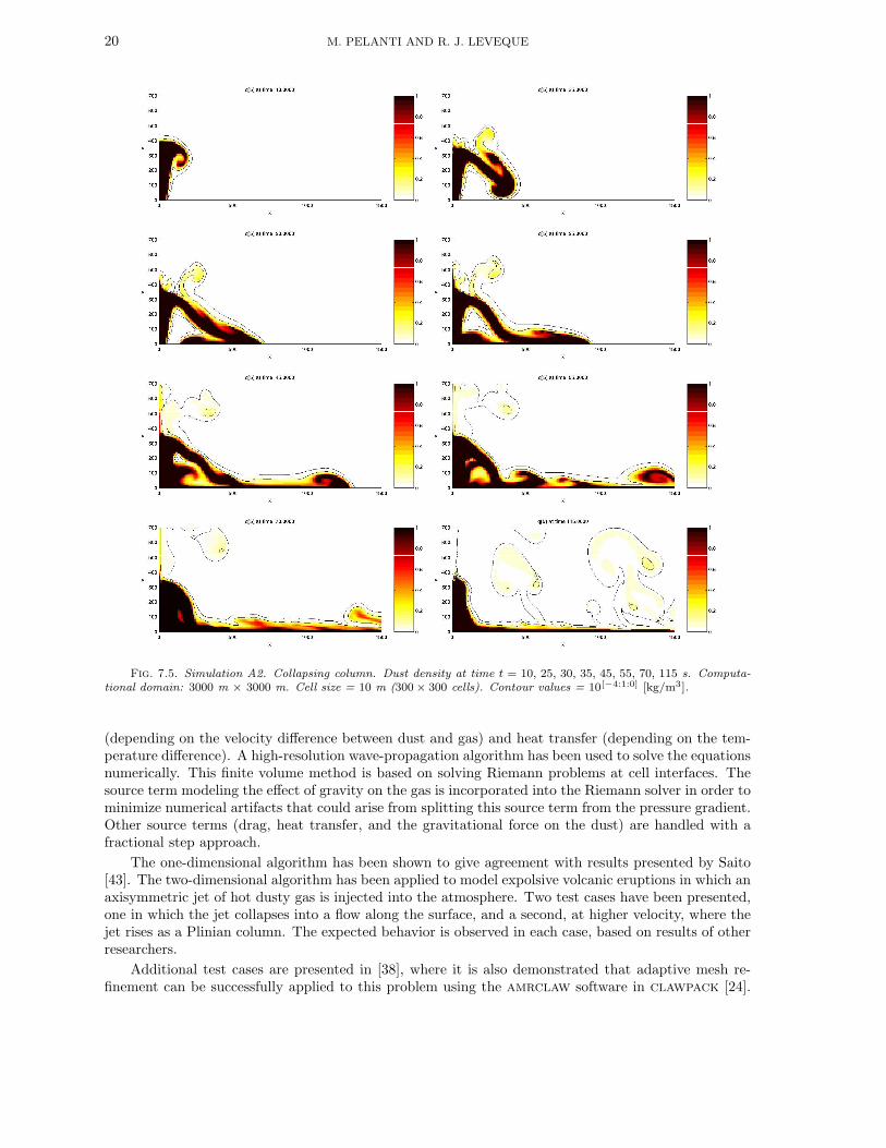
7.2.1. Simulation A2: Stationary Collapsing Column.. Figure 7.5 shows the evolution ofthe eruptive mixture as computed for simulation A2, characterized by Dv = 100m and vv = 80m/s.In agreement with [30], we can recognize the typical features of a collapsing volcanic column, that is,fountain building above the volcanic vent, radially spreading pyroclastic flow, material recycling fromthe collapsed column back into the fountain, and rising of ash plumes from the pyroclastic flow. Atabout 10 s and 400m above the vent the two-phase flow jet loses its vertical thrust, and begins to forma collapsing column. After the collapsed column has hit the ground, material starts being recycled intothe fountain. As the time evolves the impact distance from the vent decreases and the column tends tostabilize with a steady narrow shape (as observed in [30]).

In Figure 7.6 we display results computed on two different grid resolutions (cell size = 10 m on theleft, and cell size = 5 m on the right). We can see that a smaller cell size produces a longer runout ofthe pyroclastic flow and a smaller thickness, but there is no notable difference in the fountain heightand in the dynamics of the collapse. The significant difference in the location of the flow head on theground can be in part related to the type of free-slip boundary condition used, though the same effectof the grid resolution has been observed also in [10], where a no slip boundary condition is employed.

In Figure 7.7 we highlight the features of the recirculation region displaying a contour plot of thedust density together with the gas velocity vector field, as computed on the finest grid.

Relating our results with those in [30], we see good agreement between plots of physical quantities.In particular, the column height and the column impact distance are comparable. There is a differencein the length of the runout of the pyroclastic flow, which is larger in our computations. This is notsurprising, since we use a free slip boundary condition on the ground, whereas in [30] a no slip conditionis used (consistent with the fact that their model contains viscous terms).

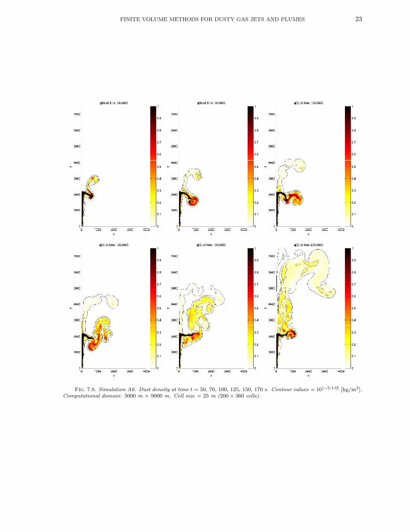
7.2.2. Simulation A6: Transitional/Plinian Column.. Figure 7.8 shows the results for Simu-lation A6, which has the same vent diameterDv = 100m as A2, but a greater exit velocity, vv = 200m/s.The increase in the jet velocity (keeping Dv fixed) generates a much more buoyant column, which inthis case appears of transitional/Plinian type, consistently with the observations in [30]. This columnreaches a height of about 2200m, and then begins to form a radially suspended flow with some materialrising buoyantly on the top of it, and other material attempting instead to collapse. The eruptive mix-ture later develops as a buoyant column. Our plots show qualitative agreement with those displayed in[30], and in particular the column height is about the same.

8. Conclusions and extensions. We have considered a model for dusty gas flow that consists ofthe compressible Euler equations for the gas coupled to a similar (but pressureless) system of equationsfor the mass, momentum, and energy of the dust. These sets of equations are coupled via drag terms


Fig. 7.5. Simulation A2. Collapsing column. Dust density at time t = 10, 25, 30, 35, 45, 55, 70, 115 s. Computa-tional domain: 3000 m × 3000 m. Cell size = 10 m (300× 300 cells). Contour values = 10[−4:1:0] [kg/m3].

(depending on the velocity difference between dust and gas) and heat transfer (depending on the tem-perature difference). A high-resolution wave-propagation algorithm has been used to solve the equationsnumerically. This finite volume method is based on solving Riemann problems at cell interfaces. Thesource term modeling the effect of gravity on the gas is incorporated into the Riemann solver in order tominimize numerical artifacts that could arise from splitting this source term from the pressure gradient.Other source terms (drag, heat transfer, and the gravitational force on the dust) are handled with afractional step approach.

The one-dimensional algorithm has been shown to give agreement with results presented by Saito[43]. The two-dimensional algorithm has been applied to model expolsive volcanic eruptions in which anaxisymmetric jet of hot dusty gas is injected into the atmosphere. Two test cases have been presented,one in which the jet collapses into a flow along the surface, and a second, at higher velocity, where thejet rises as a Plinian column. The expected behavior is observed in each case, based on results of otherresearchers.

Additional test cases are presented in [38], where it is also demonstrated that adaptive mesh re-finement can be successfully applied to this problem using the amrclaw software in clawpack [24].


Fig. 7.6. Simulation A2. Comparison between two different grid resolutions. Dust density at time t = 10, 30, 40, 50s. Left: ∆x = 10 m, Right: ∆x = 5 m. Contour values = 10[−5:.5:2] [kg/m3].

Some preliminary computations in three space dimensions are also presented in [38] and compared tothe two-dimensional axisymmetric results. Three dimensional modeling over realistic topography suchas Mount St. Helens is currently being investigated with an extension of this code.


Fig. 7.7. Simulation A2. Dust density contours and gas velocity vector field at t = 30 s. Contour values = 10[−5:.4:2]

[kg/m3]. Computational domain: 2000 m × 1000 m. Cell size = 5 m (400× 200 cells).

Because the speed of sound in a dusty gas is much lower than in a pure gas (see Section 2.2),volcanic jets can easily be supersonic and hence the jet can exhibit complex internal shock structures[20]. Some numerical study of this structure is presented in [38], and compared with some examplesconsidered in the work of Ongaro and Neri [36]. In a joint research project with these researchers, weare continuing our study of volcanic jets using the methodology described in this paper. Further resultswill be presented elsewhere [37].


Fig. 7.8. Simulation A6. Dust density at time t = 50, 70, 100, 125, 150, 170 s. Contour values = 10[−5:1:0] [kg/m3].Computational domain: 5000 m × 9000 m. Cell size = 25 m (200× 360 cells).


REFERENCES

[1] N. Andrianov and G. Warnecke. The riemann problem for the baer-nunziato two-phase flow model. J. Comput.Phys., 195:434–464, 2004.

[2] D. Bale, R. J. LeVeque, S. Mitran, and J. A. Rossmanith. A wave-propagation method for conservation laws andbalance laws with spatially varying flux functions. SIAM J. Sci. Comput., 24:955–978, 2002.

[3] N. Botta, R. Klein, S. Langenberg, and S. Ltzenkirchen. Well balanced finite volume methods for nearly hydrostaticflows. J. Comput. Phys., 196:539–565, 2004.

[4] F. Bouchut and F. James. Duality solutions for pressureless gases, monotone scalar conservation laws, and unique-ness. Commun. Math. Phys., 24:2173–2189, 1999.

[5] D. A. Calhoun, P. Colella, and R. J. LeVeque. chombo-claw software.http://www.amath.washington.edu/ calhoun/demos/ChomboClaw.

[6] P. Cargo and A.-Y. LeRoux. Un schema equilibre adapte au modele d’atmosphere avec termes de gravite. C. R.Acad. Sci. Paris Sr. I Math., 318:73–76, 1994.

[7] S. Chapman and T. G. Cowling. The Mathematical Theory of Nonuniform Gases. Cambridge University Press,1970.

[8] G. Dal Maso, P. G. LeFloch, and F. Murat. Definition and weak stablity of nonconservative products. J. Math.Pures Appl., 74:483–548, 1995.

[9] S. Dartevelle, W. I. Rose, J. Stix, K. Kelfoun, and J. W. Vallance. Numerical modeling of geophysical granularflows: 2. Computer simulations of plinian clouds and pyroclastic flows and surges. Geochem. Geophys. Geosyst.,5(8), 2004. doi:10:1029/2003GC000637.

[10] F. Dobran, A. Neri, and G. Macedonio. Numerical simulation of collapsing volcanic columns. J. Geophys. Res.,98:4231–4259, 1993.

[11] D. A. Drew and S. L. Passman. Theory of Multicomponent Fluids. Springer, 1998.[12] L. Gosse. A well-balanced flux-vector splitting scheme designed for hyperbolic systems of conservation laws with

source terms. Comput. Math. Appl., 39:135–159, 2000.[13] L. Gosse. A well-balanced scheme using non-conservative products designed for hyperbolic systems of conservation

laws with source terms. Math. Models Meth. Appl. Sci., 11:339–365, 2001.[14] J. M. Greenberg and A. Y. LeRoux. A well-balanced scheme for the numerical processing of source terms in

hyperbolic equations. SIAM J. Numer. Anal., 33:1–16, 1996.[15] F. H. Harlow and A. A. Amsden. Numerical calculation of multiphase fluid flow. J. Comput. Phys., 17:19–52, 1975.[16] A. Harten. High resolution schemes for hyperbolic conservation laws. J. Comput. Phys., 49:357–393, 1983.[17] M. Ishii. Thermo-fluid Dynamic Theory of Two-phase flow. Eyrolles, Paris, 1975.[18] S. Jin. A steady-state capturing method for hyperbolic systems with geometrical source terms. Math. Model Num.

Anal., 35:631–645, 2001.[19] B. Khouider and A. J. Majda. A high resolution balanced scheme for an idealized tropical climate model. preprint,

2004.[20] S. W. Kieffer and B. Sturtevant. Laboratory studies of volcanic jets. J. Geophys. Res., B10(89):8253–8268, 1984.[21] J. G. Knudsen and D. L. Katz. Fluid Mechanics and Heat Transfer. McGraw-Hill, New York, 1958.[22] J. O. Langseth and R. J. LeVeque. A wave-propagation method for three-dimensional hyperbolic conservation laws.

J. Comput. Phys., 165:126–166, 2000.[23] P. G. LeFloch and A. E. Tzavaras. Representation of weak limits and definition of non-conservative products. SIAM

J. Math. Anal., 30:1309–1342, 1999.[24] R. J. LeVeque. clawpack software. http://www.amath.washington.edu/~claw.[25] R. J. LeVeque. Wave propagation algorithms for multi-dimensional hyperbolic systems. J. Comput. Phys., 131:327–

353, 1997.[26] R. J. LeVeque. Balancing source terms and flux gradients in high-resolution Godunov methods: The quasi-steady

wave-propagation algorithm. J. Comput. Phys., 146:346–365, 1998.[27] R. J. LeVeque. Finite Volume Methods for Hyperbolic Problems. Cambridge University Press, 2002.[28] R. J. LeVeque. The dynamics of pressureless dust clouds and delta waves. J. Hyperbolic Diff. Eq., 1:315–327, 2004.[29] H. Miura and I. I. Glass. On a dusty-gas shock-tube. In Proceedings of the Royal Society of London. Series A,

Mathematical and Physical Sciences, volume 382, pages 373–388, 1982.[30] A. Neri and F. Dobran. Influence of eruption parameters on the thermofluid dynamics of collapsing volcanic columns.

J. Geophys. Res., 99:11833–11857, 1994.[31] A. Neri and G. Macedonio. Numerical simulation of collapsing volcanic columns with particles of two sizes. J.

Geophys. Res., 101:8153–8174, 1996.[32] A. Neri, G. Macedonio, D. Gidaspow, and T. Esposti Ongaro. Multiparticle simulation of collapsing volcanic columns

and pyroclastic flows. VSG Report No. 2001-2, Volcano Simulation Group, Istituto Nazionale di Geofisica eVulcanologia, 2001.

[33] A. Neri, A. Di Muro, and M. Rosi. Mass partition during collapsing and transitional columns by using numericalsimulations. J. Volcanol. Geotherm. Res., 115:1–18, 2002.

[34] A. Neri, T. Esposti Ongaro, G. Macedonio, and D. Gidaspow. Multiparticle simulation of collapsing volcanic columnsand pyroclastic flows. J. Geophys. Res., B4(108):1–22, 2003.

[35] A. Neri, P. Papale, and G. Macedonio. The role of magma composition and water content in explosive eruptions, 2.Pyroclastic dispersion dynamics. J. Volcanol. Geotherm. Res., 87:95–115, 1998.


[36] T. Esposti Ongaro and A. Neri. Flow patterns of overpressured volcanic jets. European Geophysical Society, XXIVGeneral Assembly, The Hague, 19-23 April 1999.

[37] T. Esposti Ongaro, M. Pelanti, A. Neri, and R. J. LeVeque. Structure and dynamics of underexpanded volcanicjets: a comparative study using two numerical multiphase flow models. in preparation.

[38] M. Pelanti. Wave Propagation Algorithms for Multicomponent Compressible Flows with Applications to VolcanicJets. PhD thesis, University of Washington, 2005.

[39] P. L. Roe. Approximate Riemann solvers, parameter vectors, and difference schemes. J. Comput. Phys., 43:357–372,1981.

[40] L. Sainsaulieu. An Euler system modeling vaporizing sprays. In A. L. Kuhl, J.-C. Leger, A. A. Borisov, andW. A. Sirignano, editors, Dynamics of Heterogeneous Combustion and Reacting Systems (Progress Series inAeronautics and Astronautics), volume 152, pages 280–305. American Institute of Aeronautics and Astronautics,Washington DC, 1993.

[41] L. Sainsaulieu. Finite volume approximation of two-phase fluid flows based on an approximate Roe-type Riemannsolver. J. Comput. Phys., 121:1–28, 1995.

[42] L. Sainsaulieu. Traveling waves solution of convection-diffusion systems whose convection terms are weakly noncon-servative: application to the modeling of two-phase fluid flows. SIAM J. Appl. Math., 55:1552–1576, 1995.

[43] T. Saito. Numerical analysis of dusty-gas flows. J. Comput. Phys., 176:129–144, 2002.[44] G. A. Valentine and K. H. Wohletz. Numerical models of Plinian eruption columns and pyroclastic flows. J. Geophys.

Res., 94:1867–1887, 1989.[45] G. B. Wallis. One-Dimensional Two-Phase Flow. McGraw-Hill, New York, 1969.[46] K. H. Wohletz, T. R. McGetchin, M. T. Sanford II, and E. M. Jones. Hydrodynamic forming of caldera-forming

eruptions: numerical models. J. Geophys. Res., 89:8269–8285, 1984.[47] K. H. Wohletz and G. A. Valentine. Computer simulations of explosive volcanic eruption. In M. P. Ryan, editor,

Magma transport and storage, pages 113–135, New York, 1990. John Wiley.[48] H. C. Yee. Upwind and symmetric shock-capturing schemes. NASA Ames Technical Memorandum 89464, 1987.

Documents

HIGH-RESOLUTION FINITE VOLUME METHODS FOR DUSTY …faculty.washington.edu/rjl/pubs/dustyjet/sisc063501.pdfHIGH-RESOLUTION FINITE VOLUME METHODS FOR DUSTY GAS JETS AND PLUMES MARICA