High Performance Commercial Building Systems

William L. Carroll Ernest Orlando Lawrence Berkeley National Laboratory June 2004

RESEM-CA Final Project Report Element 2 – Life Cycle Tools Project 2.2 – Retrofit Tools Task 2

HPBCS E2P2.2T3LBNL - 57775

California Energy Commission Public Interest Energy Research Program

Acknowledgement This work was supported by the California Energy Commission, Public Interest Energy Research Program, under Contract No. 400-99-012 and by the Assistant Secretary for Energy Efficiency and Renewable Energy, Building Technologies Program of the U.S. Department of Energy under Contract No. DE-AC03-76SF00098.

DISCLAIMER This document was prepared as an account of work sponsored by the United States Government. While this document is believed to contain correct information, neither the United States Government nor any agency thereof, nor The Regents of the University of California, nor any of their employees, makes any warranty, express or implied, or assumes any legal responsibility for the accuracy, completeness, or usefulness of any information, apparatus, product, or process disclosed, or represents that its use would not infringe privately owned rights. Reference herein to any specific commercial product, process, or service by its trade name, trademark, manufacturer, or otherwise, does not necessarily constitute or imply its endorsement, recommendation, or favoring by the United States Government or any agency thereof, or The Regents of the University of California. The views and opinions of authors expressed herein do not necessarily state or reflect those of the United States Government or any agency thereof, or The Regents of the University of California. This report was prepared as a result of work sponsored by the California Energy Commission (Commission). It does not necessarily represent the views of the Commission, its employees, or the State of California. The Commission, the State of California, its employees, contractors, and subcontractors make no warranty, express or implied, and assume no legal liability for the information in this report; nor does any party represent that the use of this information will not infringe upon privately owned rights. This report has not been approved or disapproved by the Commission nor has the Commission passed upon the accuracy or adequacy of the information in this report.

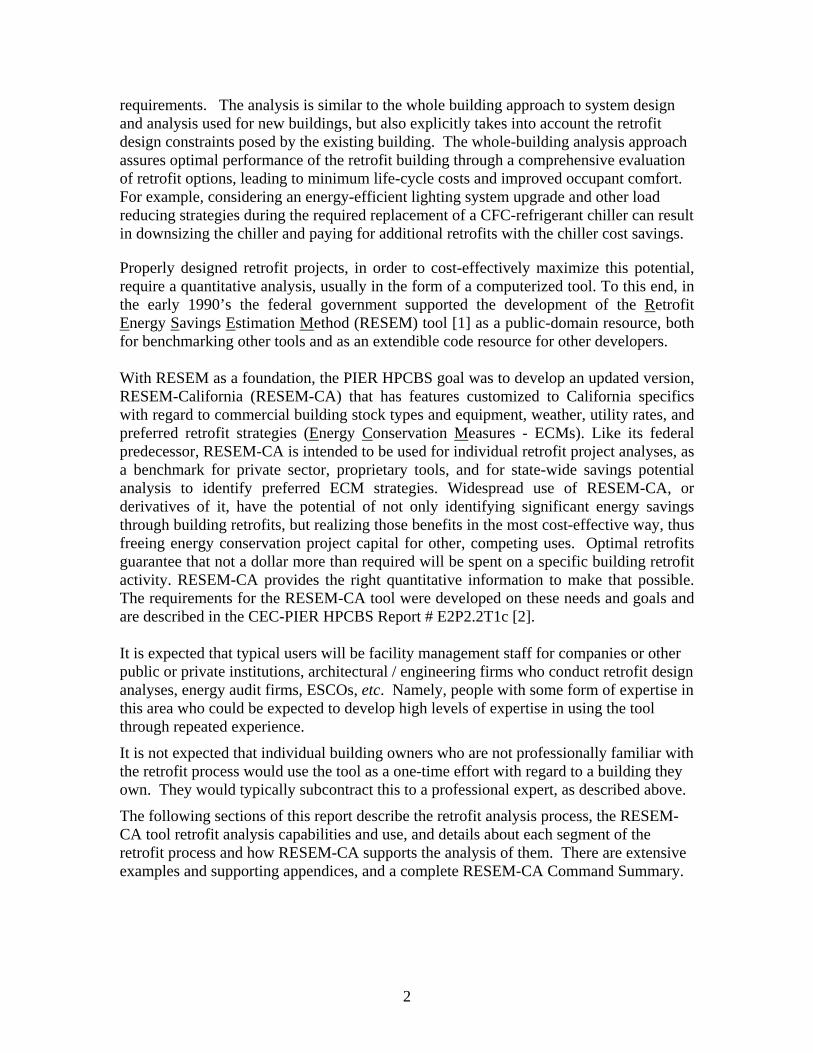
Table of Contents 1. Abstract ....................................................................................................................... 1 2. Introduction................................................................................................................. 1 3. Conceptual Model of the Retrofit Analysis Process ................................................... 3 4. The RESEM-CA Tool .................................................................................................. 3

4.1. Major Features .................................................................................................... 3 4.2. Running the RESEM-CA Program..................................................................... 4 4.3. Components Library ........................................................................................... 6 4.4. ECM Descriptions and Retrofit Analysis ........................................................... 6 4.5. Utility Cost Calculations..................................................................................... 7 4.6. Life-Cycle Cost Analysis - Economic Assumptions .......................................... 8 4.7. Weather data ....................................................................................................... 8 4.8. The RESegy Simulation Engine ......................................................................... 8 4.9. Prototype Buildings ............................................................................................ 9

5. Example Retrofit Analysis: Energy and Economic Savings ..................................... 10 6. Conclusions and recommendations .......................................................................... 12

6.1. Conclusions....................................................................................................... 12 6.2. Commercialization Potential............................................................................. 12 6.3. Recommendations............................................................................................. 13

7. References ................................................................................................................. 14 Appendix A: Milestones and Deliverables........................................................................ 15 Appendix B: Building Components Library...................................................................... 16 Appendix C: Typical Base Case Building Input ............................................................... 19 Appendix D: Retrofit Savings Analysis ............................................................................. 22 Appendix E: Utility Rates and Cost Calculations............................................................. 25 Appendix F: Life-Cycle Cost Analysis and Economic Assumptions................................. 27 Appendix G: Weather data................................................................................................ 30 Appendix H: RESegy Validation....................................................................................... 31 Appendix I: RESEM-CA Command Summary .................................................................. 33 Appendix J: List of Acronyms ........................................................................................... 44

1. Abstract This document is the final deliverable for Project 2.2 - Retrofit Tools, in the California Energy Commission Public Interest Energy Research Program for High Performance Commercial Building Systems (PIER-HPCBS). The objective of Project 2.2 is to deliver an updated and California-Customized retrofit analysis tool based on the earlier federally funded RESEM (Retrofit Energy Savings Estimation Method) tool [1]. Specific tasks to accomplish this were identified in PIER HPCBS Report # E2P2.2T1c [see references], and addressed (a) modernization, (b) enhancement of basic analysis methods and capabilities, (c) adding, modifying, or updating databases for California building types, systems, components, utility rate structures, and weather.

2. Introduction No matter what energy conservation gains can be made in new building design and operation, energy-efficient retrofits of even a part of the large size of the existing building stock will always provide a large savings potential. This is true even if the energy savings potential for a single retrofitted building is smaller than the energy savings potential of a single newly designed building. Given a useful life of 30 to 50 years or more, it is inevitable that a constructed building will undergo a variety of changes over that time. These changes are motivated by numerous circumstances including changes in occupancy and use, renovation, maintenance, newly available technologies, mandated equipment changes (e.g., removing CFC-refrigerant chillers), and the desire to improve the overall performance of an existing building. Aside from routine maintenance and simple modifications, these changes generally involve considerable effort in renovation or retrofit activities. Non-residential building retrofits offer an enormous potential for energy savings in existing buildings.

A major development in the retrofit market in recent years has been the provision of project analysis, design, and even financing through energy services providers such as utilities and Energy Service Companies (ESCOs). This is perceived as a major business opportunity, and the ESCO world is growing rapidly. ESCOs typically conduct their own analysis to both maximize their competitiveness in project bidding, and to maximize their share of the savings revenue stream. Such analyses with ESCO "biases" can lead to sub-optimal projects. Clients, whether public or private, can be at a disadvantage in project negotiations if they do not have the ability to conduct their own independent, unbiased analysis. There is thus an important role for the state of California to play to help achieve the most of the retrofit market potential in a fair and economically optimal way, with flexible, understandable, accepted methods and processes, and cost-effective tools. This will help to level the playing field between the client and the Service providers and / or ESCOs.

A renovation/retrofit project requires, analogous to the design and construction of a new building, a process of planning, design, construction, and commissioning. However, since renovation/retrofit is for an existing building, supporting analysis processes and tools tailored to this specific process would more effectively support its unique analysis

1

requirements. The analysis is similar to the whole building approach to system design and analysis used for new buildings, but also explicitly takes into account the retrofit design constraints posed by the existing building. The whole-building analysis approach assures optimal performance of the retrofit building through a comprehensive evaluation of retrofit options, leading to minimum life-cycle costs and improved occupant comfort. For example, considering an energy-efficient lighting system upgrade and other load reducing strategies during the required replacement of a CFC-refrigerant chiller can result in downsizing the chiller and paying for additional retrofits with the chiller cost savings.

Properly designed retrofit projects, in order to cost-effectively maximize this potential, require a quantitative analysis, usually in the form of a computerized tool. To this end, in the early 1990’s the federal government supported the development of the Retrofit Energy Savings Estimation Method (RESEM) tool [1] as a public-domain resource, both for benchmarking other tools and as an extendible code resource for other developers. With RESEM as a foundation, the PIER HPCBS goal was to develop an updated version, RESEM-California (RESEM-CA) that has features customized to California specifics with regard to commercial building stock types and equipment, weather, utility rates, and preferred retrofit strategies (Energy Conservation Measures - ECMs). Like its federal predecessor, RESEM-CA is intended to be used for individual retrofit project analyses, as a benchmark for private sector, proprietary tools, and for state-wide savings potential analysis to identify preferred ECM strategies. Widespread use of RESEM-CA, or derivatives of it, have the potential of not only identifying significant energy savings through building retrofits, but realizing those benefits in the most cost-effective way, thus freeing energy conservation project capital for other, competing uses. Optimal retrofits guarantee that not a dollar more than required will be spent on a specific building retrofit activity. RESEM-CA provides the right quantitative information to make that possible. The requirements for the RESEM-CA tool were developed on these needs and goals and are described in the CEC-PIER HPCBS Report # E2P2.2T1c [2]. It is expected that typical users will be facility management staff for companies or other public or private institutions, architectural / engineering firms who conduct retrofit design analyses, energy audit firms, ESCOs, etc. Namely, people with some form of expertise in this area who could be expected to develop high levels of expertise in using the tool through repeated experience.

It is not expected that individual building owners who are not professionally familiar with the retrofit process would use the tool as a one-time effort with regard to a building they own. They would typically subcontract this to a professional expert, as described above.

The following sections of this report describe the retrofit analysis process, the RESEM-CA tool retrofit analysis capabilities and use, and details about each segment of the retrofit process and how RESEM-CA supports the analysis of them. There are extensive examples and supporting appendices, and a complete RESEM-CA Command Summary.

2

3. Conceptual Model of the Retrofit Analysis Process RESEM is not simply a building energy simulation engine, but a broad-based analysis environment with components that provide all capabilities needed for a complete retrofit analysis, including default building prototype generation, base line building specification, energy simulations, retrofit specification and selection for creating a modified building, and comparative LCC savings analysis.

This conceptual model for the RESEM analysis process can be expanded into the following sequence of specific steps that the user must go through to complete a savings analysis:

• Define a base building • Conduct base building analysis:

• Simulate energy • Calculate annual operating cost (utility + O&M + other annual recurring costs,

see Appendix E.) • Select ECMs (or ECM-bundles) (see definitions for ECM and ECM-bundle

objects below, see Appendix D) • Apply ECMs or ECM-bundles to a copy of the base building to produce a

Modified building • Calculate aggregated 1st and annual recurring cost(s) for Modified building

• Conduct Modified building analysis: • Simulate energy • Calculate annual operating cost (utility + O&M + other annual recurring costs,

see Appendix E.) • Perform differential Life-Cycle Cost (ΔLCC) Analysis based on user inputs for

the Base Case and Modified buildings for (1) component first costs, and (2) LCC economic scenario assumptions (see Appendix F).

Subsequent sections in the main body of this report define the specific terms used above and summarize RESEM capabilities that support these steps. Many of those sections in turn have supporting appendices that describe the analysis methodology in even greater detail.

4. The RESEM-CA Tool

4.1. Major Features RESEM-CA has characteristics that make it well suited to the different use scenarios discussed above, and appear to be unique among known tools that are claimed to have some kind of retrofit analysis capability: • A batch analysis process approach based on the iterative paradigm: prepare input file

-> run analysis -> examine output -> refine input -> rerun. This sequence is fast and flexible using ASCII text input and output files.

3

• There is a very rich command set that is described in the “Command Summary” Appendix I. Examples throughout this report will demonstrate how these commands can be used to define objects: components, buildings, composite ECMs of any complexity, utility rate tariffs, economic scenarios, and to direct retrofit analysis sequences of any length using these objects.

• The object implementation is one of hierarchical containment: All objects of a particular type each have a unique name. All higher-level container object types are described in terms of named, pre-defined lower-level component types. The lowest-level components are defined in the Component Library object where they can be referenced. This object reference approach is a major strategy that provides great flexibility and allows for the easy definition and modification of higher-level objects – which is directly designed to support ECM definition and analysis.

• Objects can be easily defined and saved in and accessed from multiple input files and re-loaded from them, and thus can evolve to become “storage libraries” for those objects that can be selected reused for any analysis project. No object definitions are internal to the program. All object storage is in the input files.Utility rate schedules are a good example.

• The input and output files provide complete documentation of an analysis, which can be extracted and put into spreadsheets, other reports, etc. For a single, simple analysis, a single input file could suffice. However, there can be multiple, nested input files, thus individual parts of an analysis (e.g., a component library set can be separated out and be reused to become its own storage module. This file nesting capability is a powerful feature for modularizing and managing complex projects. It is illustrated in the input examples that follow below.

• The file descriptions are all in simple ASCII text so they can be easily viewed and edited. The only support tool needed is a text editor to examine and modify inputs and access results.

• A very fast simulation engine which makes even long, involved analysis sequences execute quickly.

4.2. Running the RESEM-CA Program RESEM-CA operates on personal computers under the Microsoft Windows environment. RESEM-CA is a stand-alone tool. RESEM-CA comes bundled into a self-contained download package that is a self-extracting .EXE file with the RESEM-CA executable and supporting files, and other documentation. Further details are contained in the README file.

RESEM-CA runs in a single-batch analysis mode that reads a simple ASCII input text file. The input file contains commands that either load appropriate data, allow the definition of components and buildings, and ECMs, or that conduct parts of the analysis process. The analysis results are written to both the command window and to a .LOG file that can be accessed afterward. Other output files with error messages and extra debug information are also produced under appropriate circumstances. Since they are ASCII text files, the content of the input file(s) and the output file(s) can be edited as desired, thus altering, evolving, or expanding an analysis sequence at will. This interface approach is extremely flexible.

4

• The batch analysis process is started either with a RUN command or at the prompt in a COMMAND window (MS-Windows), or by double-clicking on the .EXE file in a Windows Explorer window. The command is the executable name:

RESEMCAv20.exe • A single primary Run Control file named “resemca00.rsm” is always loaded and

must be present (a simple example is shown below; a more complex example is provided with the distribution as a starting template for real user projects). It contains commands and object definitions that are required to perform an analysis. This file is processed sequentially, producing outputs of analysis steps, and executes until the end of the file. Most importantly, additional input files can be loaded from this primary file. Thus, as discussed above, multiple projects can be defined and stored (and thus documented) in separate input files that can be loaded as desired.

• During the analysis run the command sequence is echoed together with analysis results, to the command window and to the “resemca00.log” file. After an analysis run has been completed the .log file can be opened in a text editor and examined or further processed.

• The input file(s) can then be re-modified and this process can then be conducted iteratively as described above.

A simple example, based on object descriptions described in other sections in the body of this report is shown here: loadfile BaseBldg0.rsm wx wx\\ca\\sacramen.rmy energy BaseBldg SacramentoAP cost1 BaseBldg ucost BaseBldg > PG&E-E-A10 > PG&E-G-NR1 end ecmapply NewBldg2 BaseBldg ecmBundle1 energy NewBldg2 SacramentoAP cost1 NewBldg2 ucost NewBldg2 > PG&E-E-A10 > PG&E-G-NR1 end costlcc lcc30-01 BaseBldg NewBldg2 Each line typically consists of a command and related arguments. This example consists of the following analysis: • Load a building description file which contains a building object named “BaseBldg0”

(which is in turn read and its commands processed at this point in the input processing).

• Load a weather data file named “SacramentoAP”. • Simulate the energy use for BaseBldg0 using SacramentoAP weather. • Conduct a first cost analysis for the base building.

5

• Compute the annual utility costs for the base building using the rate schedules shown. The rate schedules are defined in files loaded lower down in the base building description file. (The “> … end” syntax allows the input of multiple objects as an argument.)

• Modify the base building using retrofit ecm’s defined in a subsidiary file to construct “NewBldg2”.

• Simulate the energy use, and determine the first cost and annual utility costs for NewBldg2.

• Conduct a ΔLCC analysis for the base and modified buildings. At each step of the analysis, results are output to the “.log” file as described above. The details for defining commands, building component, weather, and economic objects are all described in sections below. See Appendix I (Command Summary) for a complete list of commands, objects, and their arguments.

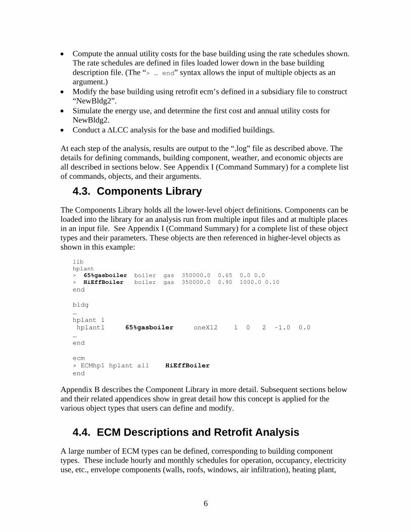
4.3. Components Library The Components Library holds all the lower-level object definitions. Components can be loaded into the library for an analysis run from multiple input files and at multiple places in an input file. See Appendix I (Command Summary) for a complete list of these object types and their parameters. These objects are then referenced in higher-level objects as shown in this example:

lib hplant > 65%gasboiler boiler gas 350000.0 0.65 0.0 0.0 > HiEffBoiler boiler gas 350000.0 0.90 1000.0 0.10 end bldg … hplant 1 hplant1 65%gasboiler oneX12 1 0 2 -1.0 0.0 … end ecm > ECMhp1 hplant all HiEffBoiler end

Appendix B describes the Component Library in more detail. Subsequent sections below and their related appendices show in great detail how this concept is applied for the various object types that users can define and modify.

4.4. ECM Descriptions and Retrofit Analysis A large number of ECM types can be defined, corresponding to building component types. These include hourly and monthly schedules for operation, occupancy, electricity use, etc., envelope components (walls, roofs, windows, air infiltration), heating plant,

6

cooling plant, and hvac systems parameters, thermal zone characterization parameters, component first costs, and others. ECM descriptions can be defined, grouped, nested, and stored in an external database file for reuse. Existing ECMs can be edited and new ECMs can be added by users. The distribution includes a small number of typical ECMs that can be used as a basis for basic studies, and as templates for the development of others by users. The retrofit analysis process was described conceptually in Section 3 above. More details on the form of ECM descriptions and the analysis process are described in Appendix D. Information sources for development of comprehensive California-specific lists of ECMs are quite varied, and include public and proprietary sources. Some are appropriate for characterizing ECM performance and cost for actual, specific products that would replace old ones in an actual retrofit project, others are statistical in nature and would be appropriate for potentials studies, etc. A useful example is: • The CEC DEER Database for Energy Efficient Resources Database for Energy

Efficient Resources (DEER) is a computer software package and an associated database which contains extensive information on selected energy-efficient technologies and measures. The DEER provides estimates of the average cost, market saturation and energy-savings potential for these technologies in residential and nonresidential applications. Specific data for each technology include size, efficiency, energy savings, saturation by climate area and by utility area, and useful life. (Available for Purchase)

• Reference: http://www.energy.ca.gov/deer/index.html The utility cost and LCC analyses that are part of the overall retrofit savings analysis process are described in more detail in subsections below and in their related appendices.

4.5. Utility Cost Calculations Utility costs are calculated from utility rate data and simulated building energy use and peak demand, analogous to calculating a utility bill. The monthly simulated consumption and peak demand for each purchased fuel type in the building are used with the rate schedule to calculate the cost. Utility rate schedules are collected in an external database with a uniform structure of billing components, which is in turn developed from other data sources that have been identified. The utility rate schedule specification capabilities are very general, and can describe complex tariffs, including Time-Of-Use (TOU) rates. More details on the analysis method and the related analysis commands are described in Appendix E.

7

4.6. Life-Cycle Cost Analysis - Economic Assumptions

The ECM life-cycle cost (LCC) savings are calculated from the ECM 1st cost(s) and discounted operation (utility) cost. It is based on a differential (Δ LCC) method which compares the ECM-modified bldg to the base case as reference. It is the LCC analysis that properly quantifies the economic tradeoff between investing in retrofitted ECMs and the time stream of savings they produce, providing the right balance. The balance point is affected both by the ratio of 1st costs to annual utility and operating costs and by the long-term economic assumptions. Economic assumptions needed for the LCC analysis include projections for energy cost increases and discount rates over a future time stream (typically 25 years, updated by NIST annually) that is relevant for the particular project being analyzed. The econimic life of an ECM is assumed to be the same as the project analysis lifetime. More details on the analysis method including information sources and references, and specification of LCC scenario parameters are contained in Appendix F.

4.7. Weather data A set of RESEM-CA weather data for the 16 standard CZ2 locations (developed for use in California Title 24 Building Performance Standards analyses) have been processed into RESEM format bin data and are provided as part of the RESEM-CA distribution. These are stored in a standard location relative to the RESEM-CA executable program on the computer hard disk. More details on the analysis method are described in Appendix G.

4.8. The RESegy Simulation Engine At the heart of the RESEM-CA analysis capability is the RESegy building energy simulation engine which models the energy use of a specified building for a specified climate. This engine was developed for the original federal RESEM project, and enhanced during this effort. It is based on a bin-method approach which represents a reasonable tradeoff between speed and accuracy that is designed to be fast, flexible, and to support the component-based approach to building specification developed during this project and described throughout this report. The next major section of this report will show typical out reports generated by RESegy.

RESegy Validation

A part of this development effort was a validation exercise of RESegy. The CEC-PIER HPCBS Report # E2P2.2T2b [3] documents the validation of RESEM-CA electrical and gas energy consumption calculations to determine the effectiveness of this tool for retrofit

8

design and analysis. The analysis compares patterns of monthly and annual energy consumption as calculated by RESEM-CA and by DOE2.1E and tries to explore and/or explain the differences, if any. A spreadsheet-based tool was developed to facilitate and document the results of the extensive comparison analysis.

In most cases there is substantial agreement in the results of RESEM-CA and DOE2.1E. In cases where there are differences, there is potential to improve agreement with minor algorithmic changes without compromising the speed of the RESEM-CA tool that is necessary for extensive parametric retrofit analysis. On the whole, this validation study indicates that RESEM is a suitable tool for retrofit analysis.

As a result of this study some factors (incident solar radiation, outside air film coefficient, IR radiation) have been identified where there is a possibility of algorithmic improvements. These would have to be made in a way that does not sacrifice the speed of the tool, which is necessary for extensive parametric search of optimum ECM measures.

Appendix H describes the validation study and results in more detail.

4.9. Prototype Buildings Building Prototypes can be developed manually using the very flexible building description syntax. The typical building presented in Appendix C is an example. It is possible to very quickly modify descriptions as in the example to describe other buildings based on a specification. A prototype specification then is an actual BLDG description. It can be fully described in the input, or it can be loaded from a saved external file.

Potential California building prototypes information sources include:

• NEOS Corporation. 1993. Technology Energy Savings: Summary of Building Prototype Descriptions and Detailed Measures Tables. Prepared for the California Conservation Inventory Group by NEOS Corporation, Sacramento, CA.

• Huang, J., H. Akbari, L. Rainer, R. Ritschard. 1991. 481 Commercial Building Prototypes for 20 Urban Market Areas. GRI-90/0326, LBL-29798, Prepared for the Gas Research Institute by Lawrence Berkeley National Laboratory, Berkeley, CA.

• California Energy Commission Comprehensive End-Use Survey (CEUS). CEUS is a comprehensive buildings characteristics survey sponsored by the CEC. This survey has been contracted out to major California electric utilities for their service territories. The most recent characteristics are in the PG&E “1999 Commercial Building Survey Report,”

http://www.pge.com/docs/pdfs/biz/energy_tools_resources/ building_survey/CEUS_1999.pdf

• The LBNL CEC-PIER Project Cal Arch has incorporated the CEUS characteristics into a WWW-based benchmarking tool: http://poet.lbl.gov/cal-arch/

9

5. Example Retrofit Analysis: Energy and Economic Savings

This section provides example results of ECM and LCC analyses for the simple base case building described in Appendix C, using the components described in Appendix B and the example ECMs described in Appendix D. This is a simple example. It is possible to build up input files to conduct very complex and / or extensive retrofit analysis projects. All of these results are output to the file “resemca00.log”. That file has to be renamed by the user before any subsequent analyses to avoid it being over-written. • Sacramento: Base Case Energy Consumption and Utility costs energy BaseBldg SacramentoAP RESEM Version 2.01 - Report Date: 06/08/04-14:43:50 Project: BaseBldg Month elec elec gas gas Kwhrs demand therms demand 1/-1 44035.7 134.78 3146.1 6.29 2/-1 41434.1 141.92 2767.4 6.33 3/-1 47890.3 157.35 3038.6 6.38 4/-1 48999.1 165.66 2794.3 6.39 5/-1 55196.4 196.71 2810.7 6.38 6/-1 57240.9 203.13 2646.9 6.35 7/-1 66205.2 211.55 2692.9 6.34 8/-1 63840.1 203.56 2715.9 6.35 9/-1 57137.3 208.49 2680.2 6.36 10/-1 54123.8 183.92 2853.3 6.41 11/-1 46664.6 157.46 2898.7 6.45 12/-1 44290.3 134.77 3125.9 6.30 Total 627058.0 211.55 34170.9 6.45 ucost BaseBldg UtilRate: PG&E-E-A10 99815.18 UtilRate: PG&E-G-NR1 34400.75 total: 134215.93

• Sacramento: 1 ECM at a time; LCC-ranked The results show Simple Payback (SPB), Savings to Investment ratio (SIR), Conservation Index (CI: ratio of retrofit First Cost net present value to the fuel savings net present value, and Δ LCC). Note that negative Δ LCC values are not only valid, but desirable. It means that the ECM-modified building configuration has a lower LCC than the base case, which is what is desired. The best ECMs have the largest negative Δ LCC valaues and are at the bottom of the list. These results should not be considered definitive; they depend in a complex way on all of the assumptions about retrofit costs and life-cycle cost scenarios, and can change for different assumptions. Procedurally, these results were obtained from a single batch run where all analyses were specified, in Appendix D and the “BaseBldg0.rsm” example input file.

10

The results for each analysis include Simple Payback and Savings to Investment Ratio (both independent of long-term economic assumptions), echo of user-specified long-term economic assumptions object name, and Conservation Index and Δ LCC. Terms are defined in Appendix F. ecmapply NewBldg1 BaseBldg ECMwall1 costlcc BaseBldg NewBldg1: SPB: 17.55 years; SIR: 0.06; lcc30-01: CI: 15.54; LCC: -2365.09 ecmapply NewBldg1 BaseBldg ECMroof1 costlcc BaseBldg NewBldg1: SPB: 12.74 years; SIR: 0.08; lcc30-01: CI: 15.49; LCC: -25811.80 ecmapply NewBldg1 BaseBldg ECMwind1 costlcc BaseBldg NewBldg1: SPB: 3.38 years; SIR: 0.30; lcc30-01: CI: 15.41; LCC: -100211.87 ecmapply NewBldg1 BaseBldg ECMzlgts0 costlcc BaseBldg NewBldg1: SPB: 1.28 years; SIR: 0.78; lcc30-01: CI: 15.82; LCC: -222770.81 ecmapply NewBldg1 BaseBldg ECMhp1 costlcc BaseBldg NewBldg1: SPB: 3.78 years; SIR: 0.26; lcc30-01: CI: 14.75; LCC: -532545.22 ecmapply costlcc BaseBldg NewBldg1: SPB: 1.42 years; SIR: 0.71; lcc30-01: CI: 16.23; LCC: -559204.37 ecmapply NewBldg1 BaseBldg ECMsyst1 costlcc BaseBldg NewBldg1: SPB: 5.30 years; SIR: 0.19; lcc30-01: CI: 16.76; LCC: -1221973.23

• Sacramento: Bundle of all ECMs Note in these results that the electricity and gas consumption and utility costs are drastically reduced by the ECMs, far outweighing their initial installation costs. ecmapply NewBldg2 BaseBldg ecmBundle1 ECMapply: ecmBundle1 ecmbundle ECMapply: ECMzlgts0 zonelgts

11

ECMapply: ECMwind1 window ECMapply: ECMhp1 hplant ECMapply: ECMcp1 cplant ECMapply: ECMsyst1 system cost1 NewBldg2 383000.00 energy NewBldg2 SacramentoAP Month elec elec gas gas Kwhrs demand therms demand Total 184560.0 71.8 18905.6 4.2 ucost NewBldg2 UtilRate: PG&E-E-A10 31213.01 UtilRate: PG&E-G-NR1 19179.70 total: 50392.71 costlcc BaseBldg NewBldg2: SPB: 4.57 years; SIR: 0.22; lcc30-01: CI: 17.31; LCC: -2092196.50 6. Conclusions and recommendations

6.1. Conclusions

The RESEM-CA tool technical capabilities have been demonstrated to be able to quantitatively analyze the cost and energy impacts of different candidate ECM options and to identify the effects of multiple ECM combination packages for a project. This is its core intended function.

6.2. Commercialization Potential RESEM-CA commercialization potential has a number of facets, including:

• RESEM-CA could serve as a public-domain benchmark for other tools or for broad potential studies intended to develop general retrofit design guidelines by either public entities or utilities.

• In addition to providing the tool as a complete packaged single-entity executable program, making the various functionalities (e.g. core simulation engine, ECM identification and ranking, etc.) available as individual modules could expand the usefulness of the analysis methods by incorporation into yet other tools from other developers (see Cal-Arch opportunity discussed below).

• The migration of RESEM-CA to the web services environment is an attractive possible approach to accomplishing that end. The recommendations immediately following also address this issue.

• As an example, service and energy providers, ESCOs are major players, profit motivated and competitive: they want to maximize both their competitive advantage in winning a project bid and at the same time their negotiating advantage with the client. They will (and already are) developing their own proprietary analysis

12

techniques and procedures. However, in a competitive environment, they would probably not only accept and support standardized, public domain procedures such as RESEM-CA because of the known quality and underlying uniformity (and to calibrate their proprietary variations), but even beyond that, ESCOs have the potential to be collaborators in future work, even in the public sector, for reasons described above.

6.3. Recommendations Identifying data sources (building prototypes, ECM characteristics, performance, and

cost, weather, utility rate schedules) necessary for linking to RESEM-CA to complete a retrofit analysis is a challenging issue. While a number of sources were identified, they are scattered, in different formats, and may even be private. It may not be feasible for an entity such as the CEC or a utility to try to collect this information and package and distribute it for use with the tool. A better approach would be to publish the object data schema developed for RESEM-CA. It is hoped that dissemination of these schema will motivate the owners of such data to develop data files based on the specifications and make them available for other RESEM-CA users, based on their potential commercial value to such users. If the use of the tool is desirable enough to create a market for the information in this specific form, user demand should stimulate this response.

Opportunities should be explored to integrate RESEM-CA with other tools and analysis processes. The highly integrated nature of analysis descriptions, fast analysis, and results logging makes it fast and easy to use in conjunction with Cal-Arch or other analysis tools. Specifically, with respect to Cal-Arch: (1) Cal-Arch could serve as the interface and access mechanism for the CEUS [see section 4.9 above] prototypical building templates that RESEM-CA could then analyze in real time. (2) RESEM-CA could produce an LCC-optimal ECM retrofit package and related quantitative prediction of the expected energy performance improvement and economic savings from the for a building a user was benchmarking in Cal-Arch. Even further – RESEM-CA could also compare the improvements expected from the retrofit package for the specific building to the average and / or 90% range of expected improvements for the aggregated class of cohort buildings in the Cal-Arch database.

Another opportunity is the integration of RESEM into M&V analysis processes used either by ESCOs or building owner clients to bring quantitative estimation rigor to savings verification. The predicted "back end" post-retrofit analyses could form the basis for a monitoring and savings verification tool based on ongoing comparison with actual measured post-retrofit data.

.

13

7. References The citations here are for references in the body of the report. Appendices each have separate reference citations where needed. 1. Hitchcock, R., W.L. Carroll, and B.E. Birdsall, RESEM Reference Manual, Version

1.0, LBNL-51874, July 1991.

2. “RESEM-CA: Software Specifications Document,” CEC-PIER HPCBS Report # E2P2.2T1c W. L. Carroll, and R. J. Hitchcock http://buildings.lbl.gov/hpcbs/pubs/E2P22T1c.pdf

3. “RESEM-CA: Validation and Testing,” V. Pal, W. L. Carroll, and N. Bourasssa, Lawrence Berkeley Report LBNL-52003, 2004. http://buildings.lbl.gov/hpcbs/pubs/E2P22T2b-LBNL-52003.pdf

14

Appendix A: Milestones and Deliverables

Description Start Date

Due Date

Planned Actual Planned Actual Specifications for the software modifications that will be made to the RESEM tool

7/15/00 7/15/00 2/10/01 2/10/01

RESEM model diagrams 7/15/00 7/15/00 7/12/01 8/10/01

Operational RESEM retrofit tool/testbed, including sample inputfiles and underlying databases

7/15/00 7/15/00 7/12/01 7/31/01

Enhanced RESEM Tool

Enhanced retrofit tool/tested 7/15/01 9/1/01 7/14/02 7/28/02

Report on calibration of RESEM calculation engine against DOE2.1E

1/15/02 9/30/02

9/30/02

Final RESEM Capabilities

Enhanced retrofit tool/tested 7/15/02 7/30/02 7/14/03 6/1/04

15

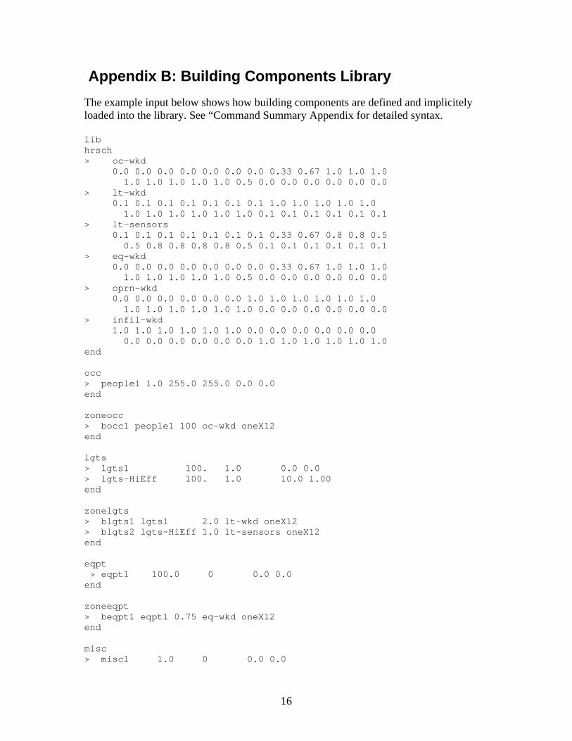
Appendix B: Building Components Library The example input below shows how building components are defined and implicitely loaded into the library. See “Command Summary Appendix for detailed syntax. lib hrsch > oc-wkd 0.0 0.0 0.0 0.0 0.0 0.0 0.0 0.33 0.67 1.0 1.0 1.0 1.0 1.0 1.0 1.0 1.0 0.5 0.0 0.0 0.0 0.0 0.0 0.0 > lt-wkd 0.1 0.1 0.1 0.1 0.1 0.1 0.1 1.0 1.0 1.0 1.0 1.0 1.0 1.0 1.0 1.0 1.0 1.0 0.1 0.1 0.1 0.1 0.1 0.1 > lt-sensors 0.1 0.1 0.1 0.1 0.1 0.1 0.1 0.33 0.67 0.8 0.8 0.5 0.5 0.8 0.8 0.8 0.8 0.5 0.1 0.1 0.1 0.1 0.1 0.1 > eq-wkd 0.0 0.0 0.0 0.0 0.0 0.0 0.0 0.33 0.67 1.0 1.0 1.0 1.0 1.0 1.0 1.0 1.0 0.5 0.0 0.0 0.0 0.0 0.0 0.0 > oprn-wkd 0.0 0.0 0.0 0.0 0.0 0.0 1.0 1.0 1.0 1.0 1.0 1.0 1.0 1.0 1.0 1.0 1.0 1.0 0.0 0.0 0.0 0.0 0.0 0.0 > infil-wkd 1.0 1.0 1.0 1.0 1.0 1.0 0.0 0.0 0.0 0.0 0.0 0.0 0.0 0.0 0.0 0.0 0.0 0.0 1.0 1.0 1.0 1.0 1.0 1.0 end occ > people1 1.0 255.0 255.0 0.0 0.0 end zoneocc > bocc1 people1 100 oc-wkd oneX12 end lgts > lgts1 100. 1.0 0.0 0.0 > lgts-HiEff 100. 1.0 10.0 1.00 end zonelgts > blgts1 lgts1 2.0 lt-wkd oneX12 > blgts2 lgts-HiEff 1.0 lt-sensors oneX12 end eqpt > eqpt1 100.0 0 0.0 0.0 end zoneeqpt > beqpt1 eqpt1 0.75 eq-wkd oneX12 end misc > misc1 1.0 0 0.0 0.0

16

> misc2 1.0 0 1.0 1.0 end zonemisc > bmisc1 misc2 1.0 eq-wkd oneX12 end dhw > dhw1 1.0 0.0 0.0 > dhw2 1.0 1.0 1.0 end zonedhw > bdhw1 dhw1 1.0000 oneX24 oneX12 end infil > infil1 0.5 0.0 1.0 end tstat end wall > wall-R11 0.09 E 0.7 0.9 0.0 0.0 > WallCons 0.05 E 0.7 0.7 0.0 1.0 end roof > roof-R11 0.09 12 0.7 0.9 0 0.0 0.0 > RoofCons 0.04 12 0.4 0.9 0 0.0 1.0 end window > wind-1pane 500. 1.1 0.84 1.0 0.0 0.0 > WindCons 500. 0.5 0.40 1.0 0.0 3.0 end hplant > 65%gasboiler boiler gas 350000.0 0.65 0.0 0.0 > HiEffBoiler boiler gas 350000.0 0.90 1000.0 0.10 > #2oilboiler boiler #2oil 350000.0 0.65 0.0 0.0 end cplant > COP2.8centrifugal centr elec 125.0 2.80 0.0 0.0 > COP4.0centrifugal centr elec 100.0 4.00 10000.0 200.0 end system > cvct0 cvct 10000.0 0.40 0 0.0 0 0.3 0.4 1 0.0 55.0 0 70.0 40.0 55.0 105.0 0.0 0.0 > vav1 vav 10000.0 0.25 1 70.0 0 0.3 0.4 1 0.0 55.0 1 70.0 40.0 55.0 105.0 10000.0 5.0 end bldgmischt

17

> radianthtr 10000. 1000.0 1.0 end bldgmiscel > ParkingLotLights 0.1 1000.0 100.0 > Parking0 0.0 0.0 0.0 end end

18

Appendix C: Typical Base Case Building Input The example below defines a typical five-zone 10,000 square foot one story building. It refers by name to components defined in the library (Appendix B). See “RESEM-CA Command Summary” Appendix I for detailed syntax. bldg BaseBldg bldgsch oprn-wkd oprn-wkd oprn-wkd hplant 1 hplant1 65%gasboiler oneX12 1 0 2 -1.0 0.0 cplant 1 cplant1 COP2.8centrifugal hplant1 oneX12 1 0 2 -1.0 0.0 system 5 hvac1 cvct0 cplant1 oneX12 hplant1 oneX12 hvac2 cvct0 cplant1 oneX12 hplant1 oneX12 hvac3 cvct0 cplant1 oneX12 hplant1 oneX12 hvac4 cvct0 cplant1 oneX12 hplant1 oneX12 hvac5 cvct0 cplant1 oneX12 hplant1 oneX12 mischt 0 miscel 0 zone zNorth 1250.0 10.0000 system hvac1 3500.0 15.0 nocc 1 bocc1 1.0 nlgts 1 blgts1 1.0 neqpt 1 beqpt1 1.0 nmisc 0 ndhw 1 hplant1 bdhw1 1.0 tstat tstat0 infil infil0 infil-wkd mass 2.0 nwall 1 wall-R11 1000.0 0.0 90.0 nwind 1 wind-1pane 1 0.0 nroof 1 roof-R11 1250.0 0.0 0.0 nwind 0 end zone zEast 1250.0 10.0000 system hvac2 8000.0 15.0 nocc 1 bocc1 1.0 nlgts 1 blgts1 1.0

19

neqpt 1 beqpt1 1.0 nmisc 0 ndhw 1 hplant1 bdhw1 1.0 tstat tstat0 infil infil0 infil-wkd mass 2.0 nwall 1 wall-R11 1000.0 90.0 90.0 nwind 1 wind-1pane 1 0.0 nroof 1 roof-R11 1250.0 0.0 0.0 nwind 0 end zone zSouth 1250.0 10.0000 system hvac3 6200.0 15.0 nocc 1 bocc1 1.0 nlgts 1 blgts1 1.0 neqpt 1 beqpt1 1.0 nmisc 0 ndhw 1 hplant1 bdhw1 1.0 tstat tstat0 infil infil0 infil-wkd mass 2.0 nwall 1 wall-R11 1000.0 180.0 90.0 nwind 1 wind-1pane 1 0.0 nroof 1 roof-R11 1250.0 0.0 0.0 nwind 0 end zone zWest 1250.0 10.0000 system hvac4 7500.0 15.0 nocc 1 bocc1 1.0 nlgts 1 blgts1 1.0 neqpt 1 beqpt1 1.0 nmisc 0 ndhw 1 hplant1 bdhw1 1.0 tstat tstat0

20

infil infil0 infil-wkd mass 2.0 nwall 1 wall-R11 1000.0 270.0 90.0 nwind 1 wind-1pane 1 0.0 nroof 1 roof-R11 1250.0 0.0 0.0 nwind 0 end zone zCore 5000.0 10.0 system hvac5 6200.0 15.0 nocc 1 bocc1 1.0 nlgts 1 blgts1 1.0 neqpt 1 beqpt1 1.0 nmisc 0 ndhw 1 hplant1 bdhw1 1.0 tstat tstat0 infil infil0 infil-wkd mass 2.0 nwall 0 nroof 1 roof-R11 5000.0 0.0 0.0 nwind 0 end end

21

Appendix D: Retrofit Savings Analysis

Specifying ECMs Single-ECM objects: • Contain specific ECM characteristics used to instantiate a single actual ECM • Can be loaded from and saved into external DataBase files. • Reference(s) by Name to component / construction objects that are used to

characterize the BLDG modifications due to applying the ECM (and are in LIB / BLDG Object lists. • This object reference approach is a major strategy: ALL ECMs are

described in terms of pre-defined component types. • 1st Cost of retrofit components: materials, labor, rebates are defined in the library

component specifications • Examples (see “Command Summary Appendix for detailed syntax)

ecm > ECMzlgts0 zonelgts all blgts2 > ECMwall1 wall all WallCons > ECMwind1 window all WindCons > ECMroof1 roof all RoofCons > ECMinfil infil all infil1 > ECMtstat tstat all tstat_dbsch > ECMhp1 hplant all HiEffBoiler > ECMcp1 cplant all COP4.0centrifugal > ECMsyst1 system all vav1 end

The ECM “Bundle” object: • A specified list of defined ECMs or ECMBundles • Bundles can be nested. The idea is to build up complex retrofits from simpler 1-type

ECM descriptions. May also work for “building up” a complex ECM of a SINGLE MajorType out of simpler pieces, e.g. schedule change + capacity change + …

• Example (see “Command Summary Appendix for detailed syntax) ecmbundle ecmBundle1 > ECMzlgts0 > ECMwind1 > ECMhp1 > ECMcp1 > ECMsyst1

end The Savings Analysis Process

• Define a Base BLDG • Base BLDG analysis

• Simulate energy • Calculate annual operating cost (utility + O&M + other annual recurring costs,

see Appendix E.)

22

• Calculate building First Cost • Select a defined ECM or ECM_bundle (or bundles) (see definitions for ECM and

ECM-bundle objects below) • Apply ECMs / ECMbundles to Base BLDG to produce Modified BLDG • Modified BLDG analysis

• Simulate energy • Calculate annual operating cost (utility + O&M + other annual recurring costs,

see Appendix E.) • Calculate building First Cost

• Calculate differential Aggregated 1st cost (the cost of the retrofits) and annual recurring cost(s) (utility bills, maintenance, etc. ) between Modified BLDG and Base BLDG

• Perform Life-Cycle Cost (LCC) Analysis based on all cost components for both Base BLDG and Modified BLDG, and on LCC economic scenario assumptions (see Appendix F).

• ECM Apply method

• Modify a copy of BLDG description: • Modify Action: replace all targeted (by name) objects) with replacement

object. • Action Modifiers

• “all”: • Specified target object Name

• Bundle Apply • LOOP through bundle list of single-ECMs

• Recursively evaluate nested bundles • BLDG modifications are sequentially accumulated.

• ECM precedence ordering isw managed manually by the way the user constructs ECM and ECMBundle lists.

• Complete ECM analysis example (see “Command Summary Appendix for detailed

syntax). The ucost, cost1, and costlcc analysis commands are described in more detail in appropriate Appendices.

energy BaseBldg SacramentoAP ucost BaseBldg > PG&E-E-A10 > PG&E-G-NR1 end cost1 BaseBldg ecmapply NewBldg2 BaseBldg ecmBundle1 cost1 NewBldg2 energy NewBldg2 SacramentoAP ucost NewBldg2 > PG&E-E-A10 > PG&E-G-NR1 end

23

costlcc lcc30-00 BaseBldg NewBldg2 costlcc lcc30-01 BaseBldg NewBldg2 costlcc lcc30-DOE2003 BaseBldg NewBldg2

Possible future enhancements to the ECM savings analysis process include: • A repeating process that can identify the best bundle out of a large number of

automatically selected of ECM bundles from comprehensive ECM databases. This would be useful for generating predefined regional- and building-type specific LCC-optimal bundles for widespread application, or for conducting broad policy analysis studies. This would produce a ranked / LCC-Minimum retrofit list. The sequenced could be built up using existing definition and analysis Command sequences.

24

Appendix E: Utility Rates and Cost Calculations Utility costs are calculated from utility rate data and simulated building energy use and peak demand, analogous to calculating a utility bill. Utility rate schedules are collected in an external database, which is in turn developed from other data sources that have been identified. There are two important challenges:

• In general, rate structures can be very complex. • They tend to have a wide range of component data structures and / or algorithmic

calculation procedures. • They change regularly, and need to be updated. • The only true authoritative sources are the utilities that issue them.

Utility rate schedule object Typical examples in the RESEM syntax are shown below. These were extracted directly from published tariffs from the respective utilities. These definitions reference library names that are provided in a separate input file. See “Command Summary” Appendix for detailed syntax. urate name PG&E-E-A10 ftype elec kWh kW consblocks 1 0 –1 WinterCons1 WinterCons1 WinterCons1 SummerCons1 SummerCons1 SummerCons1 SummerCons1 SummerCons1 SummerCons1 SummerCons1 WinterCons1 WinterCons1 dmdblocks 1 0 -1 PGE-E-A10-DmdBlk1 ratchet 0 0 0 fixedchg PGE-E-A10-Fixed1 minchg 0 taxrate 0 end urate name PG&E-E-A10TOU ftype elec kWh kW consblocks 1 0 –1 PGE-E-A10TOUWinter1 PGE-E-A10TOUWinter1 PGE-E-A10TOUWinter1 PGE-E-A10TOUWinter1 PGE-E-A10TOUSummer1 PGE-E-A10TOUSummer1 PGE-E-A10TOUSummer1 PGE-E-A10TOUSummer1 PGE-E-A10TOUSummer1 PGE-E-A10TOUSummer1 PGE-E-A10TOUWinter1 PGE-E-A10TOUWinter1 dmdblocks 1 0 -1 PGE-E-A10-DmdBlk1 ratchet 0 0 0 fixedchg PGE-E-A10-Fixed2 minchg 0 taxrate 0 end urate name PG&E-G-NR1 ftype gas therm Btu/hr consblocks 2 0 4000 PGE-G-NR1WinterCons1 PGE-G-NR1WinterCons1 PGE-G-NR1WinterCons1 PGE-G-NR1SummerCons1

25

PGE-G-NR1SummerCons1 PGE-G-NR1SummerCons1 PGE-G-NR1SummerCons1 PGE-G-NR1SummerCons1 PGE-G-NR1SummerCons1 PGE-G-NR1SummerCons1 PGE-G-NR1WinterCons1 PGE-G-NR1WinterCons1 4000 –1 PGE-G-NR1WinterCons2 PGE-G-NR1WinterCons2 PGE-G-NR1WinterCons2 PGE-G-NR1SummerCons2 PGE-G-NR1SummerCons2 PGE-G-NR1SummerCons2 PGE-G-NR1SummerCons2 PGE-G-NR1SummerCons2 PGE-G-NR1SummerCons2 PGE-G-NR1SummerCons2 PGE-G-NR1WinterCons2 PGE-G-NR1WinterCons2 dmdblocks 0 ratchet 0 0 0 fixedchg PGE-G-NR1-Fixed1 minchg 0 taxrate 0 end

California utility rate schedules sources: • Utilities are the only authoritative primary source. • Secondary sources may cost less, be more convenient, and be good enough for the

type of analysis to be done (e.g., real project or abstract potentials analysis). • Example Source: LBNL Tariff Analysis Project (T.A.P.). The Tariff Analysis

Project (T.A.P.), is a comprehensive data warehouse of electric combined with a variety of query and analytical tools. T.A.P. contains a growing library of hundreds of tariffs, from over a hundred utilities, for residential, commercial-industrial, agricultural and public sector customers. A generic data model has been developed to concisely represent all varieties of tariff structures, capturing seasonal charges, time-of-use rates, and complex block structures. REFERENCE: http://tariffs.lbl.gov/

26

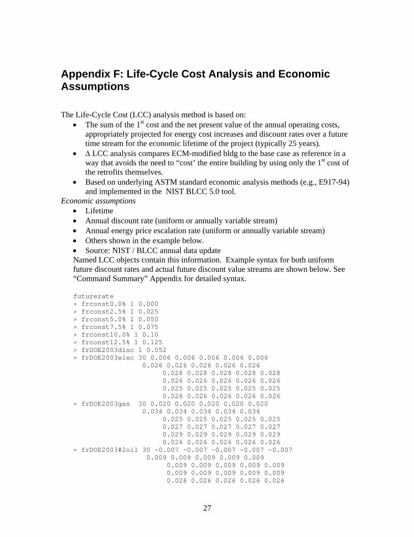
Appendix F: Life-Cycle Cost Analysis and Economic Assumptions The Life-Cycle Cost (LCC) analysis method is based on:

• The sum of the 1st cost and the net present value of the annual operating costs, appropriately projected for energy cost increases and discount rates over a future time stream for the economic lifetime of the project (typically 25 years).

• Δ LCC analysis compares ECM-modified bldg to the base case as reference in a way that avoids the need to “cost’ the entire building by using only the 1st cost of the retrofits themselves.

• Based on underlying ASTM standard economic analysis methods (e.g., E917-94) and implemented in the NIST BLCC 5.0 tool.

Economic assumptions • Lifetime • Annual discount rate (uniform or annually variable stream) • Annual energy price escalation rate (uniform or annually variable stream) • Others shown in the example below. • Source: NIST / BLCC annual data update Named LCC objects contain this information. Example syntax for both uniform future discount rates and actual future discount value streams are shown below. See “Command Summary” Appendix for detailed syntax. futurerate > frconst0.0% 1 0.000 > frconst2.5% 1 0.025 > frconst5.0% 1 0.050 > frconst7.5% 1 0.075 > frconst10.0% 1 0.10 > frconst12.5% 1 0.125 > frDOE2003disc 1 0.052 > frDOE2003elec 30 0.006 0.006 0.006 0.006 0.006 0.026 0.026 0.026 0.026 0.026 0.028 0.028 0.028 0.028 0.028 0.026 0.026 0.026 0.026 0.026 0.025 0.025 0.025 0.025 0.025 0.026 0.026 0.026 0.026 0.026 > frDOE2003gas 30 0.020 0.020 0.020 0.020 0.020 0.034 0.034 0.034 0.034 0.034 0.025 0.025 0.025 0.025 0.025 0.027 0.027 0.027 0.027 0.027 0.029 0.029 0.029 0.029 0.029 0.026 0.026 0.026 0.026 0.026 > frDOE2003#2oil 30 -0.007 -0.007 -0.007 -0.007 -0.007 0.009 0.009 0.009 0.009 0.009 0.009 0.009 0.009 0.009 0.009 0.009 0.009 0.009 0.009 0.009 0.026 0.026 0.026 0.026 0.026

27

0.025 0.025 0.025 0.025 0.025 end

lcc lcc30-01 lifetime 30 discountrate frconst7.5% loanrate 0.12 appreciationrate 0.10 financefract 0.9 maintfract 0.02 resalecredit 0.0 incometaxrate 0.3 proptaxrate 0.020 insrate 0.005 fuelincrate 3 elec frconst7.5% gas frconst12.5% #2oil frconst10.0% end lcc lcc30-DOE2003 lifetime 30 discountrate frDOE2003disc loanrate 0.12 appreciationrate 0.10 financefract 0.9 maintfract 0.02 resalecredit 0.0 incometaxrate 0.3 proptaxrate 0.020 insrate 0.000 fuelincrate 3 elec frDOE2003elec gas frDOE2003gas #2oil frDOE2003#2oil end References

• “Life-Cycle Costing Manual,” NIST Handbook 135 (1995 Edition) February 1996.

• “Energy Price Indices and Discount Factors for Life-Cycle Cost Analysis,” NISTIR 85-3273-18, Rev. 4/03, April 2003.

Possible future enhancements

• Explore generalization of the LCC analysis to include renewables / green / environmental metrics or rating systems for buildings (e.g., REEP, LEED, ATHENA, etc). Some of these attempt to calculate a quantitative scale of generalized performance that can be used to compare and rank buildings. Candidate methods include: • ISO 14040 series standards for Life Cycle Assessment (LCA)

28

• ASTM E1765-98, Standard practice for Multi-attribute decision analysis of investments related to buildings and systems.

• Multi-Criteria Decision Making Tool (MCDM-23): D. Balcomb, IEA SH&C Task 23

• Add ESPC / 3rd party financing economics analysis. • Based on NIST BLCC 5.0 methodology

29

Appendix G: Weather data A set of RESEM-CA weather data for the 16 standard CZ2 locations have been processed into RESEM format bin data and are provided as part of the RESEM-CA distribution. These are stored in a standard location relative to the RESEM-CA executable program on the computer hard disk.

Weather data files processed into the RESEM format can be loaded as follows. The double-backslash “\\” notation is required when specifying the weather file pathname. wx wx\\ca\\fresnoap.rm2 wx wx\\ca\\arcatafa.rm2 wx wx\\ca\\losangel.rm2 wx wx\\ca\\sacramen.rmy wx wx\\ca\\sandiego.rmy wx wx\\ca\\sanfranc.rm2 wx wx\\ca\\sunnyval.rmy

Weather data is only used in energy simulation analyses, and is referenced by weather city name, not weather file name. Weather city names can be found and used as shown below.

wxsummary FresnoAPS ArcataFAA LosAngelesAPS SacramentoAP SanDiegoAP SanFranciscoAP SunnyvaleMoffettNAS

energy BaseBldg SacramentoAP

30

Appendix H: RESegy Validation

This section summarizes the results of an extended comparison of simulation results of the core engine of the RESEM tool benchmarked against a widely accepted simulation tool, DOE2.1E. Reference [2] contains a complete, detailed description of the comparison.

The validation and testing of RESEM algorithms was carried out in two phases:

1. Comparison of monthly heating and cooling loads, including peak heating and cooling loads, as computed by RESEM and DOE2.1E. The comparisons were performed on a simple base-case building "Analytical Base Case" with controlled variations in it to explore the predictions of load components of each program.

2. Comparison of the changes in electrical and gas energy consumption computed by RESEM and DOE2.1E when a selected list of ECMs was applied to a typical 5-zone building design of average performance with a VAV system, a central chiller and boiler (ECM base case).

This summary focuses on the latter comparisons, which are very important because RESEM is a retrofit analysis tool and it is important to know how various ECM retrofit measures affect the energy and economic performance of the building.. The Figure below shows the comparison between the monthly electrical and gas energy use computed by RESEM and DOE2.1E for the ECM base case building in Fresno. We use the annual total electrical and gas consumption values as the predicted performance metrics to be compared The electrical energy use includes the energy consumption for cooling and direct plug loads. The gas consumption is for heating. Annual electrical energy use computed by RESEM and DOE2.1E is not significantly different, though monthly values show some difference. RESEM overestimates the annual gas consumption by 20% as compared with DOE2.1E. RESEM shows a slightly bigger monthly swing in electrical and gas energy use as compared with DOE2.1E.

El e c Ene r gy

0.0

5000.0

10000.0

15000.0

20000.0

25000.0

30000.0

35000.0

40000.0

R-Kwhr s

D-Kwhr s

Ga s- The r ms

0.0

200.0

400.0

600.0

800.0

1000.0

1200.0

1400.0

R-ther ms

D-ther ms

31

Additionally, it was found that even with differences in some of the load components, RESEM does provide similar “bottom line” results in predictions of the overall effect of ECMs on the change in the building energy performance from a baseline. This is of critical importance for correct retrofit analysis. On the whole, this validation study indicates that RESEM is a promising tool for retrofit analysis. As a result of this study some factors (incident solar radiation, outside air film coefficient, IR radiation) have been identified where there is a possibility of algorithmic improvements. These would have to be made in a way that does not sacrifice the speed of the tool. Reference “RESEM-CA: Validation and Testing,” V. Pal, W. L. Carroll, and N. Bourasssa, Lawrence Berkeley Report LBNL-52003, 2004. http://buildings.lbl.gov/hpcbs/pubs/E2P22T2b-LBNL-52003.pdf

32

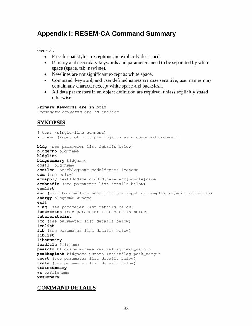
Appendix I: RESEM-CA Command Summary General:

• Free-format style – exceptions are explicitly described. • Primary and secondary keywords and parameters need to be separated by white

space (space, tab, newline). • Newlines are not significant except as white space. • Command, keyword, and user defined names are case sensitive; user names may

contain any character except white space and backslash. • All data parameters in an object definition are required, unless explicitly stated

otherwise. Primary Keywords are in bold Secondary Keywords are in italics

SYNOPSIS ! text (single-line comment) > … end (input of multiple objects as a compound argument) bldg (see parameter list details below) bldgecho bldgname bldglist bldgsummary bldgname cost1 bldgname costlcc basebldgname modbldgname lccname ecm (see below) ecmapply newBldgName oldBldgName ecm[bundle]name ecmbundle (see parameter list details below) ecmlist end (used to complete some multiple-input or complex keyword sequences) energy bldgname wxname exit flag (see parameter list details below) futurerate (see parameter list details below) futureratelist lcc (see parameter list details below) lcclist lib parameter list details below) (seeliblist libsummary loadfile filename peakcfm bldgname wxname resizeflag peak_margin peakhcplant bldgname wxname resizeflag peak_margin ucost (see parameter list details below) urate (see parameter list details below) uratesummary wx ame wxfilenwxsummary

COMMAND DETAILS

33

! (comment line text) to end of line only; cannot be embedded in the middle of most command data blocks

> … end (input of multiple objects) used for building up a compound argument of an arbitrary number of objects of the expected type. NOTE: The keywords for which this syntax is valid are shown explicitly below. bldg Note: Secondary keywords and parameter data must be specified in the order shown) bldgname bldgsch wkdayopschname satopschname sunopschname hplant nhplants [integer] hplantname libhpname monhsch nunit[integer] staged[integer] optype[integer] pumpelec[kW] pilotheat[Btu/hr] (repeat) ... cplant ncplants[integer] cplantname libcpname htgpidname moncsch nunit[integer] staged[integer] optype[integer] pumpelec[kW] ctower[kW] (repeat) ... system nsysts [integer] name libsysname clgpidname moncsch htgpidname monhsch (repeat) ... mischt nmischt [integer] libname nunit [integer] hrschid htgpidname (repeat) ... miscel nmiscel [integer] libname

34

nunit [integer] hrschidname monschidname (repeat) ... zone...end (see zone input definition below) zone...end (repeat for additional zones) ... end bldgecho bldgname bldglist (no argument) bldgsummary bldgname cost1 bldgname costlcc basebldgname modbldgname lccname ecm > ecmname1 type target replacename > ecmname2 type target replacename > ... end ecmname type: valid type name from list: bldgmiscel bldgmischt cplant ecmbundle hplant infil roof system tstat wall window zonedhw zoneeqpt zonelgts zonemisc zoneocc target: {valid target name for component type, or "all"} replacename: valid replacement name for component type ecmapply (Note: Secondary keywords and parameter data must be specified in the order shown) newBldgName oldBldgName {ecm or ecmbundle} name ecmbundle > ecmname1 > ecmname2 > ...

35

> ecmbundlename1 (can be nested to any level) > ... end ecmlist (no argument) end (used to complete some multiple-input or complex keyword sequences) energy (run RESegy energy simulation)

bldgname wxname

exit stop input processing and exit program flag /* debug, error reporting & action flags */ flagcode [letter from list] a /* */ b /* Bldg dump*/ c /* Cplant dump*/ d e /* return(-1) on Errors */ f // FirstCost g /* eGy1shot simulation EGY_REC dump*/ h /* Hplant dump*/ i /* Inputs dump */ j k l /* Loads dump */ m // ECMapply modification details n // auto ECM analysis o // base case analysis p /* Peak lds */ q r /* energy end-use Reports */ s /* Systs dump*/ t u /* Util costs */ v /* Verbose on errors */ w x y z /* Zones dump*/ flagval [0 or 1] futurerate (Note: Secondary keywords and parameter data must be specified in the order shown) fratename nyears [integer] numvalue1 numvalue2 ... numvalue-nyears futureratelist (no argument) lcc (Note: Secondary keywords and parameter data must be specified in the order shown) lccname

36

lifetime nyears [integer] discountrate futureratename loanrate numval [decimal fraction] appreciationrate numval [decimal fraction] financefract numval [decimal fraction] maintfract numval [decimal fraction] resalecredit numval [decimal fraction] incometaxrate numval [decimal fraction] proptaxrate numval [decimal fraction] insrate numval [decimal fraction] fuelincrate nrates [integer] fueltype1 futureratename1 (see urate below for valid fuel type names) fueltype2 futureratename2 ... fueltype-n futureratename-n end lcclist (no argument) lib (Note: Additional lib commands can be located wherever the user wants. Duplicate names are not allowed) typename1 > name1 parameters... > name2 parameters... > ... end typename2...end typename3...end ... end valid lib component typenames and parameters: (Note: Parameter data must be specified in the order shown) hrsch: name numval1...numval24 monsch: name numval1...numval12 occ: name parea[sqft/person] psens[Btu/hr] plat[Btu/hr] cost0[$/person] cost1[$/???] not defined zoneocc: name occidname density[sqft/person] hrschid monschid

37

lgts: name ltpwr[watt] lthtosp[decimal fraction] cost0[$/unit] cost1[$/watt] zonelgts: name lgtsidname density[watt/sqft] hrschid monschid eqpt: name eqpwr[watt] eqhood[decimal fraction] cost0[$/unit] cost1[$/watt] zoneeqpt: name eqptidname density[watt/sqft] hrschid monschid misc: name miscpwr[Btu/hr] mischood[decimal fraction] cost0[$/unit] cost1[$/Btu/hr] zonemisc: name miscidname density[Btu/hr-sqft] hrschid monschid dhw: name hwuse[gal/person-day] cost0[$/unit] cost1[$/???] (not defined) zonedhw: name dhwname density[dhwname/sqft] ?? hrschid monschid wall: name u[Btu/hr-sqft-degF] groupname

38

colcor[numval] emisIR[decimal fraction] cost0[$???] cost1[$/sqft???] roof: name u[Btu/hr-sqft-degF] code[integer] colcor[numval] emisIR[decimal fraction] plenum[integer] cost0[$] cost1[$/sqft] window: name area[sqft] u[Btu/hr-sqft-degF] emisIR[decimal fraction] shdc[decimal fraction] leakc[sqft] cost0[$] cost1[$/sqft] infil name rate0[ach] cost0[$] cost1[$/ach] tstat: name hstatsched cstatsched cost0[$] cost1[not defined] hplant: name typename (valid hplant typenames: "sum", "boiler", "furnace", "disth"}) egytype (valid egy typenames: see urate) cap[Btu/hr] eff[decimal fraction] cost0[$] cost1[$/Btu/hr] cplant: name typename (valid cplant typenames: "sum", "centr", "recip",

"screw", "absorp", "dxac", "distc"}) egytype (valid egy typenames: see urate) cap[tons] cop[numval] cost0[$] cost1[$/ton]

39

system: name systype (valid syst typenames: {"sum", "cvct", "cvvt", "vav", "sum2"}) scfm [cfm] fanpwr [watt/cfm] fanctrl [integer] econlt [degF] enth [integer] sminOA [decimal fraction] vvminair [decimal fraction] vvctrl [integer] minRH [decimal fraction] ccddt [degF] reset [integer] oahi [degF] oalo [degF] ccmdt [degF] hcddt [degF] cost0 [$] cost1 [$cfm] bldgmischt: name rate [Btu/hr] cost0 [$] cost1 [$/Btu/hr] bldgmiscel: name rate [kW] cost0 [$] cost1[$/kW] liblist (no argument) libsummary (no argument) loadfile filename [full or relative path] loadfile command can be nested in input files to any level

peakcfm (Note: Secondary keywords and parameter data must be specified in the order shown) bldgname wxname resizeflag [integer] peak_margin [decimal fraction] peakhcplant (Note: Secondary keywords and parameter data must be specified in the order shown) bldgname wxname resizeflag [integer] peak_margin [decimal fraction]

40

ucost (Note: Secondary keywords and parameter data must be specified in the order shown) bldgname nutilrates [integer] utilratename1 utilratename2 ... urate (Note: Secondary keywords and parameter data must be specified in the order shown) name ftype (valid fuel type names) {"none", "elec", "gas", "#2oil", "#6oil", "coal", "disth", "distc", "other", "hplant"} consumptionunits demandunits consblocks nblocks [integer] low-limitval hi-limitval (= -1 for last block) TOUhrsched1 ... TOUhrsched12 (12 TOU profile names, one for each month) ... next block ... last block dmdblocks nblocks [integer] low-limitval hi-limitval (= -1 for last block) TOYmonsched (1 monthly schedule name with 12 values) ... next block ... last block ratchet ratchetflag [integer] multiplier [numval] length [integer] (months) fixedchg monschedname minchg [numval] taxrate [numval] end uratesummary (no argument) wx wxfilename (full or relative path) wxsummary (no argument) zone (Note: Secondary keywords and parameter data must be specified in the order shown. Secondary keywords must be present in the input.) name area [sqft] height - floor-to-floor [ft] system systname

41

cfmrate [cfm] min_cfm_person [cfm] nocc n [integer] (for each of n:) zoneoccname (from lib) floorfraction [0 - 1.0] ... nlgts n [integer] (for each of n:) zonelgtsname (from lib) floorfraction [0 - 1.0] ... neqpt n [integer] (for each of n:) zoneeqptname (from lib) floorfraction [0 - 1.0] ... nmisc n [integer] (for each of n:) zonemiscname (from lib) floorfraction [0 - 1.0] bldghtplantname ... ndhw n [integer] (for each of n:) zonedhwname (from lib) floorfraction [0 - 1.0] bldghtplantname ... tstat tstatname (from lib) infil infilname (from lib) monschname (from lib) mass numvalue [no unit] nwall n [integer] (for each of n:) wallname (from lib) grossarea [sqft] azimuthangle [deg - CW from North] tiltangle [deg - from zenith] nwind n [integer] (for each of n:) windname (from lib) nunits leakagecoeff [sqft] ... ... nroof

42

n [integer] (for each of n:) roofname (from lib) grossarea [sqft] azimuthangle [deg - CW from North] tiltangle [deg - from zenith] nwind n [integer] (for each of n:) windname (from lib) nunits leakagecoeff [sqft] ... ... end

43

Appendix J: List of Acronyms CI Conservation Index CEUS California Commercial Building End Use Survey CZ2 California Standard Weather Zone ECM Retrofit Energy Conservation Measure ESCO Energy Service Company LCC Life-Cycle Cost ΔLCC differential life-cycle cost M&V Measurement and Verification O&M Operation and Maintenance PIER-HPCBS California Energy Commission Public Interest Energy Research

Program for High Performance Commercial Building Systems RESEM Retrofit Energy Savings Estimation Method RESEM-CA RESEM-California RESegy RESEM-CA building energy simulation engine SIR Savings to Investment ratio SPB Simple Payback

44