High-Order Accurate Methods for High-Speed Flowaero-comlab.stanford.edu/Papers/may.aiaa.05-5251.pdf · High-Order Accurate Methods for High-Speed Flow Georg May∗ and Antony Jameson†

High-Order Accurate Methods for High-Speed Flow

Georg May∗ and Antony Jameson†

This work focuses on high-order numerical schemes for conservation laws with empha-sis on problems that admit discontinuous solutions. We will investigate several enablingtechniques with the aim to construct robust methods for unstructured meshes capable ofreliably producing globally high-order accurate results even in the presence of discontinu-ities. We use spectral and pseudo-spectral schemes in connection with such techniques asGibbs-complementary reconstruction to recover high-order accuracy near discontinuities.

I. Introduction

Computational aerodynamics has been dominated by schemes which are higher than first-order accurateonly in smooth regions, where they are typically restricted to second, or perhaps third order accuracy.The presence of discontinuities in transonic aerodynamics has greatly hampered the success of high-orderaccurate methods. In the vicinity of discontinuities the typical scheme uses restrictive limiters to damp outhigh-frequency oscillatory modes. While low-order schemes have been very successful due to their robustnessand relative efficiency, many fields of research, such as aeroacoustics, large-eddy simulation (LES), andunsteady nonperiodic flow require highly accurate numerical methods. For many applications a high-orderaccurate scheme for solutions with discontinuities that retains its nominal accuracy everywhere would bequite welcome.

In this paper we will explore one possible route to such a scheme. We will start from a most promisingnew numerical scheme for unstructured meshes, namely the Spectral Difference method,1 which combineselements from finite-volume and finite-difference techniques, and is particularly attractive because of itssimple formulation and implementation.

It is well known that high-order accurate numerical schemes will produce oscillatory solutions for hyper-bolic equations with discontinuities, if these are not prevented by using nonlinear limiters. The unlimitedsolution, if stabilized by high-order diffusion, exhibits oscillations of the order of what one would expect fromGibbs’ phenomenon, if the analytical solution were to be expanded in smooth basis functions. In the absenceof instabilities and if it is not destroyed by using limiting functions, it can be conjectured that informationup to the nominal degree of accuracy is still present, in the sense established by the Gibbs-complementaryreconstruction, which has been recently developed in a different context as a means of recovering high-orderaccurate smooth representations given spectral data for discontinuous functions. We investigate the exten-sion of such methods to high-order approximations of partial differential equations. We confirm in this paperby strict measurements for nonlinear hyperbolic equations that indeed the full nominal order of accuracycan be recovered from the unlimited oscillatory solution. For the Euler equations, smooth solutions withperfect discontinuities and small absolute error are shown.

We discuss the Spectral Difference Method in section II. In section III we discuss the Gibbs complemen-tary reconstruction, and point out how the rigorous theory developed for the method relates to the contextin which it is used here. We show numerical results in section IV.

∗PhD Candidate, Department of Aeronautics and Astronautics, Stanford University, AIAA Member.†Thomas V. Jones Professor of Engineering, Department of Aeronautics and Astronautics, Stanford University, AIAA

Member.

1 of 16

American Institute of Aeronautics and Astronautics

II. The Spectral Difference Method

The spectral difference method has quite recently been proposed by Liu et al.1 and further developed byWang et al.2 We will restrict ourselves in this paper to the solution of equations of the form

∂u

∂t+∇ · F = 0 (1)

on simplices, such as triangles in two dimensions. Suppose we are given a mesh of such elements. TheSpectral Difference method uses a pseudo-spectral collocation-based reconstruction for both the dependentvariables u(x, y) and the flux function F (u) inside each element. The reconstruction for the dependentvariables can be written

u(x, y) =Nu∑j=1

Lj(x, y)uj (2)

Where L is the cardinal basis function for the given representation, and uj = u(xj , yj), where the (xj , yj)T

are collocation points. Similarly one can write for the flux function

F (x, y) =Nf∑k=1

Mk(x, y)Fk , (3)

where the Mk are the basis functions, and Fk = F (u(xk, yk)), where the (xk, yk)T are collocation points forthe fluxes. The number of collocation points, Nu and Nf , are determined by the selected accuracy. In twodimensions, for accuracy n, one needs

N =n(n + 1)

2(4)

collocation points for the reconstruction of the solution. If the solution is reconstructed to order n, the fluxnodes are interpolated to order m = n+1, because of the differentiation operation in equation 1. Figure 2 onpage 4 shows examples of one- and two-dimensional stencils.

Given the dependent variables at the collocation points uj , the solution is reconstructed in each cell andequation 2 is evaluated at flux collocation points k, i.e. with L(xk, yk). Fluxes are then evaluated usingthe reconstructed values of uk. The derivatives of these fluxes can be obtained by differentiating the basisfunction. Thus ∇ · F is obtained and evaluated at the solution collocation points using ∇Mk(xj , yj) · Fk inequation 3, and the solution can be updated via equation 1 and a time integration scheme, such as a Runge-Kutta scheme. The method is closely related to staggered grid multidomain methods, proposed by Kopriva.3

Here, in a sense, each simplex is a subdomain, and instead of tensor product forms of one-dimensional basisfunctions, we use two-dimensional collocation methods.

The key ingredient of the method is the flux evaluation of nodes located on the element boundaries,where the flux function will be multi-valued. For flux points located on edges it is necessary for discreteconservation that the normal flux component be the same for adjacent cells. This suggests the use numericalflux formulas used in standard finite-volume formulations, Fn = h(ul, ur, ν), where Fn is the normal fluxand ul and ur are the reconstructed solution variables to the left and right of the edge, and ν is the edgenormal. A schematic illustration is shown in figure 1(a) on the following page. For flux nodes on corners theoptimal treatment is still an open problem. One may compute the corner fluxes from normal fluxes on thetwo incident edges of the triangles by imposing

F · n1 = Fn1

F · n2 = Fn2 , (5)

which makes the flux unique and allows for conservation. The linear system, equation 5, can be solvedanalytically to give modified Riemann fluxes on corners that can be split into two parts, which are associated

2 of 16


(a) Flux computation for points on edges (b) Flux computation for points on corners

Figure 1. Illustration of flux computation for nodes on element boundaries.

with the two incident edges, that are used to computed the flux F . This is shown in figure 1(b). To showdiscrete conservation for the simplex in d dimensions, Td, we must show that

I =d

dt

∫Td

u dV +∫

∂Td

F · n dA = 0 (6)

is recovered in the discrete approximation based on the collocation nodes. This imposes some restrictionsas to the choice of collocation nodes. We show in the following that these restrictions can be recast in verysimple form. Suppose u can be represented by a d-dimensional polynomial of degree at most n, and F isrepresented by a d-dimensional polynomial of degree at most n + 1. We then have

I =d

dt

∫Td

u dV = −∫

Td

Nf∑k=1

∇Mk · Fk dV = −V

Nu∑j=1

wj

Nf∑k=1

∇Mk(xj) · Fk (7)

Note that all the equalities are exact by construction, provided the collocation points for u support aquadrature with weights wj , which is exact for polynomials of degree n.

Denote the elements of the differentiation matrices ∇Mk(xj) = mkj , where each mkj is a vector with dcomponents. We have

I = −V

Nf∑k=1

Nu∑j=1

wjmkj · Fk = −Nf∑k=1

w̃k · Fk (8)

We thus arrive at a modified quadrature using the flux points. The integral, however, must not depend oninterior flux points. Indeed, we can write using the definition of the new weights w̃k:

w̃k = V

Nu∑j=1

wjmkj =∫

Td

∇Mk(x) dV =∫

∂Td

Mkν dA , (9)

where ν is the outward pointing face normal on ∂Td. The second equality is exact, because ∇M is apolynomial of degree n. Suppose the collocation points of F restricted to the boundaries of the simplex

3 of 16


support a d−1-dimensional quadrature of degree n+1 for each boundary l = 1 . . . d, with weights wlm, m =

1 . . . Ne, where Ne is the number of points on the boundaries. We then have the following exact relationship:

w̃k =∫

∂Td

Mkν dA =d∑

l=1

SlNe∑

m=1

wlmMk(xm) , (10)

where Sl is the area of face l. But since Mk is an interpolation polynomial with the property Mk(xm) = δkm,this will simply pick out the weight wl

k corresponding to the flux node k. In particular it is clear that theweight w̃k for interior nodes vanish, since k 6= m for all such nodes. We finally arrive at

I = −Nf∑k=1

w̃k · Fk = −d∑

l=1

∑Ne

m=1wl

mFk(l,m) · Sl = −∫

∂Tn

F · dS (11)

In summary, then, we are free to choose any combination of collocation nodes, provided that the nodesfor u support a quadrature of the order of the interpolation n, and the restriction of the flux nodes to theboundaries supports a d − 1-dimensional quadrature of order n + 1. For the solution nodes one can chooseGauss quadrature points. Hesthaven proposed nodes based on the solution of an electrostatics problem forsimplices,4 which support both a volume and a surface integration to the required degree of accuracy. Thesenodes have been used in this work for flux collocation. Figures 2(a) and 2(b) show examples of nodeswhich use a combination of these flux nodes with Gauss nodes for the solution. Since a volume integrationis supported, we have also used staggered grids with nodes from4 for both solution and flux functions. Sucha stencil is shown in figure 2(c). For computations in one dimension Gauss and Gauss-Lobatto nodes can be

(a) Linear Triangle: (b) Quadratic Triangle (c) Cubic Triangle

Figure 2. Schematic depiction of collocation nodes for triangles.

used. No attempts have been made to optimize the choice with respect to running time. Some stencils sharepoints between flux and solution nodes, which reduces the cost of the reconstruction. One can also choose acompletely collocated set of nodes, which eliminates the reconstruction in equation 2 completely, at the costof more expensive flux scattering procedure, due to the increased number of solution nodes.

The high-order reconstruction usually allows us to use simple flux functions on element boundaries suchas a simple average with scalar dissipation. For example one can write for the normal flux component

Fn(ul, ur) =12

{(f(ul) + f(ur)

)· n− αn

(ur − ul

)}, (12)

where α is proportional to the spectral radius of the local flux Jacobian, α ∝ un +cn, where un is the velocitynormal to the edge, and cn is the local speed of sound. We have also used the CUSP construction of artificialdiffusion5 instead of the simple dissipation of equation 12, in particular for the Euler equations. Tangential

4 of 16


flux components can either be evaluated in each cell and left unchanged or averaged across cell interfacesusing an arithmetic average. For points in the interior of an element the flux function can be evaluateddirectly with the local state.

Normally limiter functions are used to promote monotonicity of numerical schemes for nonlinear con-servation laws, which can be used to prove stability and convergence. This has been done for high-ordermethods, such as the Discontinuous Galerkin method.6 As we discuss below we have explored the possibilityof recovering solutions accurate in maximum norm without the use of such limiting functions. This requiresstabilization of the numerical scheme in some appropriate fashion, certainly in the case of discontinuities.For smooth solutions, and generally for moderate orders of accuracy the high-order dissipation from thediscontinuous states at the element boundaries is usually enough to render the scheme stable. More sophisti-cated approaches such as spectral viscosity methods7 which operate explicitly on the high-frequency part ofthe spectrum could be used, and may find use in the future. For some one-dimensional results with discon-tinuities we have also used global filtering operations, such as adaptive exponential filters,8 which attenuatethe high-frequency Fourier spectrum, to stabilize the method.

III. Gibbs-Complementary Reconstruction for spectral/pseudo-spectral data

A. Basic Theory

For convenience we will present the theory for the Gibbs-complementary reconstruction for one-dimensionalfunctions. Tensor products of the relevant basis functions can be used for the multidimensional extension.Assume that N + 1 spectral coefficients bk , k = 0,. . . ,N of a piecewise-smooth function f(x), defined on aninterval, [a, b] are given, such that

fN (x) =N∑

n=0

bkφk(x) (13)

is an approximation to the original function. The functions φk represent the chosen basis, which span acertain functional space, for instance the space of polynomials of degree at most N . The coefficients bk

can be obtained by Galerkin projection or collocation. It is well known that any of these approximationswill exhibit true exponential convergence only if f is infinitely differentiable.9 For the case that f is onlypiecewise continuous, convergence in maximum norm fails completely, which is one manifestation of Gibbs’phenomenon.

In a series of papers Gottlieb and coworkers have established the possibility of recovering high-orderaccuracy in maximum norm as N →∞, i.e. the removal of Gibbs’ phenomenon associated with the spectralrepresentation of piecewise smooth functions, see10,11 and references therein. Results were obtained for bothGalerkin and Collocation types, such as the Fourier series and expansion in Chebyshev polynomials. In fact,given the first N exact spectral coefficients exponential convergence in maximum norm as N →∞ has beenproved for any subdomain [x1, x2] where the function is analytic, i.e.

maxx∈[x1,x2]

|f(x)− fN (x)| < e−αN , α > 0 , (14)

so that by juxtaposing the domains of analyticity exponential convergence can be recovered in the completeinterval. Formally the method can be summarized as follows. Suppose a projection PN (f) of the form ofequation 13 is given. For piecewise continuous functions, the maximum error of the projection will be oforder unity. Suppose now we re-project PN into another space, spanned by basis functions which we shalldenote by Ψλ

m (we anticipate here that our new basis functions will be two-parameter families). We seekconditions under which the new projection, which we denote by GM leads to an exponentially small error inmaximum norm, ||.||∞. Consider

||GMPNf − f ||∞ ≤ ||GMPNf −GMf ||∞ + ||GMf − f ||∞ (15)

5 of 16


The second term on the right-hand side measures how well the new basis is suited to approximate the originalfunction f (For the known Gibbs complementary bases one actually needs to show that this approximationconverges while both parameters of Ψλ

m are increased simultaneously). The key step is proving that the firstcomponent of the error in equation 15 on the preceding page vanishes exponentially fast. Write this term as

||GMPNf −GMf ||∞ = ||GM (PN − I)f ||∞ . (16)

In a sense we thus have a measure of the orthogonality of the new space and the part of the spectrum ofthe original projection which is not resolved. If these spaces are nearly orthogonal, or become orthogonal atan exponential rate as N is increased, meaning that the unknown high modes have very little effect on therepresentation in the new projection, the error will decrease exponentially as N →∞.

In our case, the spectral data is an approximation, obtained by a highly accurate numerical method. Thiswill affect the reconstruction in various ways. For instance stabilizing diffusion or filtering has to be addedto the spectral or pseudo-spectral method used to compute the solution, so that instead of equation 16 onehas

||GMDpPNf −GMf ||∞ = ||GM (DpPN − I)f ||∞ , (17)

where we have formally introduced a dissipation or filtering operator of order p, which will operate primarilyon the high frequency part of the original projection PN . The effect of such operators on the reconstruction isstill an open problem. Furthermore, details of the numerical implementation, such as, boundary conditions,can be expected to have a profound effect, not considered in the previous theoretical work related to theGegenbauer reconstruction.

In this work order of accuracy is most often measured by refining the mesh (h-refinement), while keepingthe spectral modes (i.e. the number of collocation points) constant in each control volume, whereas mostof the previous work has been on spectral convergence, i.e. increasing the total number of spectral modes(p-refinement). This latter point is not expected to be critical, since after all, the fixed-rate convergence ofh-refinement is a relaxation of the convergence requirement.

B. A Gibbs-Complementary Basis: The Gegenbauer Polynomials

The first basis which has been identified as Gibbs complementary to, in fact, a whole host of spectralprojections, are the Gegenbauer polynomials, Ψλ

m = Cλm, which are a subset of the Jacobi polynomials, m is

the degree of the polynomial, and λ is a second parameter. The Gegenbauer polynomials can be defined asthe polynomials, which are orthogonal on the interval [−1, 1] with the weight function w(x) = (1− x2)λ− 1

2 ,i.e. ∫ 1

−1

Cλn(x)Cλ

m(x)(1− x2)λ− 12 dx = δnmhλ

n . (18)

In the most common form the Gegenbauer polynomials are not normalized,12 and the constant hλn is given

by

hλn = 21−2λπ

Γ(n + 2λ)(n + λ)Γ2(λ)Γ(n + 1)

, (19)

where Γ(x) is the Gamma function.We will refer to the re-projection of a spectral representation onto Gegenbauer space as the Gegenbauer

reconstruction procedure. The Gegenbauer reconstruction operates on each subinterval on which the solutionis smooth. Assume for the sake of simplicity that [−1, 1] is such an interval (general intervals can be handledby appropriate scaling). It can be shown that the truncated expansion up to order M < ∞, based of theapproximation to f , i.e. the projection GMPNf

fM =M∑

n=0

g̃λmCλ

m(x) , (20)

6 of 16


where

g̃λm =

1hλ

m

∫ 1

−1

(1− x2)λ− 12 fN (x)Cλ

n(x) dx , (21)

and fN is the original projection of the general form of equation 15 on page 5, converges exponentially fastto f in maximum norm, even at discontinuities, provided the two parameters, M and λ vary linearly withN ,

M ∝ λ ∝ N , (22)

where the constants of proportionality depend on the spectral representation of fN . While the details ofthe proof are different for different spectral representations, one can roughly argue that the necessity ofvarying the parameters in this way stems from the trade-off between the obvious fact that the the order ofthe polynomials has to be increased along with the original projection to achieve spectral convergence, andthe need to maintain a reasonable degree of separation between the complement of the original projectionand the Gegenbauer space to keep the orthogonality error, equation 16, small.

C. Remarks on the Gegenbauer Basis

Despite the fact that exponential convergence can be proven there are a few well-known problems associatedwith the Gegenbauer basis, which can have a profound effect in numerical implementations. We will brieflysummarize a few points.

• The success of the reconstruction depends on the smoothness of the unknown function. More precisely,the constants of proportionality in equation 22 depend on how far the function can be extended ontothe complex plane. In the absence of such information these constants have to be estimated, and forfixed values the reconstruction might fail for certain functions.

• The Gegenbauer polynomials assume very large numerical values very quickly as the parameters areincreased. If one wishes, for example, to resolve several periods of a low-frequency oscillation, thiscan lead to large errors for intermediate orders of approximation. If a fair number of polynomials areincluded, but not enough to resolve all periods of the oscillation, the approximation will fail (just as itwould for any polynomial approximation). But because of the large amplitude of the polynomials thefailure can be catastrophic until enough modes are added to resolve the function properly. Only thenwill the error vanish exponentially fast.

• In numerical implementations the large magnitude of the Gegenbauer polynomials also amplifies theeffect of round-off errors. While the numerical values of the polynomials increase dramatically as N isincreased, the sum in equation 20, is usually of order unity, so that for large N some coefficients in thetruncated sum may need to be smaller than machine accuracy, but at the same time highly accurate torepresent the solution with small absolute errors. The shear magnitude of the Gegenbauer polynomialsagain leads to catastrophic failure for this case.

• The very nature of the Gegenbauer projection leads to difficulties, since it becomes more and moreextrapolatory as λ is increased (the weight function approaches a delta function). In the limit of λ →∞the Gegenbauer series approaches a power series, and only the function value at the midpoint of thedomain contributes to the expansion.

D. An Alternative Basis: The Freud Polynomials

Recently, the concept of robust Gibbs complements has been proposed by Tanner and Gelb.13 The additionalrequirement is that the associated weight of the new basis converge to a limit which still has an associatedset of polynomials that can serve as a basis for an exponentially convergent projection (this is not the casefor the Gegenbauer polynomials, since the weight converges to a delta function). The Freud polynomials,

7 of 16


which are orthonormal on the real line with respect to the weight w(x) = exp(−cx2n), have been proposedas an alternative to the Gegenbauer basis, and indeed in preliminary numerical experiments have provenmore benign. Unfortunately very little is known about the Freud polynomials, in particular the three-termrecurrence relation is not known analytically, which has prevented a rigorous proof that the Freud polynomialscan serve as an alternative Gibbs complementary basis. Some elements and numerical evidence, however,have been shown.13 We will use the Freud polynomials as an alternative to the Gegenbauer polynomials forcertain test problems in this work.

E. Multidimensional Extension and Edge Detection

The Gibbs-complementary reconstruction in higher dimensions is very similar to the 1D method, using atensor product form. However, since it operates on smooth subdomains, more sophisticated domain decom-position techniques and coordinate transformations will have to be used, which poses additional algorithmicchallenges. A mapping to at least quadrilateral subdomains is required, which can then be easily mapped toa square to use the tensor product basis based on Gegenbauer or Freud polynomials.

We have omitted so far the issue of identifying discontinuities. Edge detection techniques have beenproposed,14,15 and have been used as part of this work. At least in one dimension these techniques arestraight-forward and work very reliably. In essence, the edge detection mechanism used in this work is basedon the generalized Fourier conjugate sum

SσN =

N∑k=0

σ

(k

N

)(ak sin kx− bk cos kx) , (23)

where σ = 1 corresponds to the classical conjugate sum, and the coefficients ak and bk are related to thecomplex Fourier coefficients fk via fk = ak + ibk. It is known that the classical Fourier conjugate sumconverges to

− π/ log(N)SN → [f(x)] , (24)

where [f(x)] = f(x+)− f(x−). Thus it can be conveniently used to detect discontinuities, where [f(x)] 6= 0.The factors σ(x) are introduced to accelerate the convergence. Quasi one-dimensional versions of thesetechniques for higher dimensions have also been proposed. However, the best edge detection algorithm inhigher dimensions is still subject to further research.

IV. Numerical Results

A. The Spectral Difference Method for Smooth Solutions

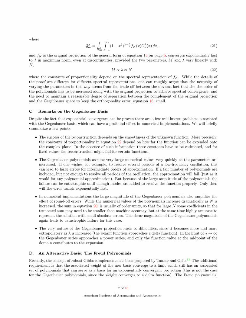
Figure 3 shows a validation of the 2D scheme on the linear advection equation

∂tu + ∂xu + ∂yu = 0 , (x, y) ∈ [0, 1]× [0, 1] (25)u(x, u, t = 0) = sin(2π(x + y)) , (26)

with periodic boundary conditions for 2nd, 3rd and 4th order accuracy. The solutions have been computedon triangular meshes, generated from structured N by N meshes by simple triangulation. The nominalaccuracy is clearly achieved for all solutions. Simple scalar diffusion for the normal fluxes has been used,while the tangential fluxes have not been averaged, but taken directly from their respective elements. Interiorflux points are evaluated directly with the reconstructed solution variables.

For validation for the Euler equations consider first the quasi-one-dimensional flow through a nozzle. Thegoverning equations are given by

∂w

∂t+

∂F

∂x+ Q = 0 , (27)

8 of 16


(a) Solution using the Spectral Difference Method on a30× 30× 2 unstructured grid

101

102

10310

−8

10−6

10−4

10−2

100

N

Err

or

3rd Order2nd Order4th Order

(b) Maximum error in mesh refinement. N is the numberof structured mesh points in each direction. There areN × N × 2 triangles .

Figure 3. Validation of the 2D Spectral Difference Method.

where

w =

ρ

ρ u

E

, F =

ρ u

ρ u2 + p

u(E + p)

, Q =1A

∂A

∂x

ρ u

ρ u2

u(E + p)

, (28)

where A is the cross-section of the domain. Figure 4 on the following page shows the steady-state entropyerror in h-refinement and p-refinement for isentropic nozzle flow as computed by the spectral differencemethod. The flow conditions have been chosen such that the nozzle exit Mach number is M = 0.3, and thenozzle geometry such that the flow is subsonic everywhere. The maximum Mach number in the throat is M ≈0.46. It can be seen that for the the 3rd order method shown in figure 4(a) the error decreases at the nominalrate in mesh refinement. For this test case no limiters have been used, and the dissipation coming from theelement boundaries is sufficient to stabilize the solution. The CUSP construction of artificial dissipation hasbeen used. For interior flux points the flux function is directly evaluated with the reconstructed solutionvariables, hence single valued.

To test the Spectral Difference Method for the 2D Euler equations, consider subsonic flow around theNACA0012 airfoil. Figure 5 shows results for a 3rd order Spectral Difference scheme at flow conditionsM = 0.3 and zero angle of attack. In figure 5(a) we show Mach number contours. We point out that thecontour plot does not use the spectral information in the solution, but merely uses a simple scattering tothe original nodes of the mesh to visualize the data. Figure 5(b) shows the distribution of entropy along theairfoil for a mesh with 2560 and 10240 triangles. For the third order scheme this corresponds to 15360 and61440 degrees of freedom (DOF), respectively, since there are six solution nodes to each triangle. Figure 5(c)compares this data with results from a finite volume scheme, which employs the CUSP scheme with a SLIPdata reconstruction,5 and uses the triangles as control volumes. Note that these are merely isolated resultsand do not represent an attempt to carry out a mesh refinement study. The mesh has not been isotropicallyrefined, but merely ”best-practice” meshes have been used. Note that the entropy error for the spectraldifference scheme with 15,360 DOF is roughly equal to the entropy error of the finite-volume scheme with

9 of 16


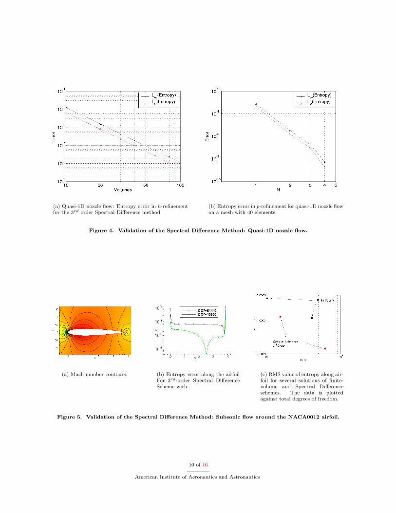
(a) Quasi-1D nozzle flow: Entropy error in h-refinementfor the 3rd order Spectral Difference method

(b) Entropy error in p-refinement for quasi-1D nozzle flowon a mesh with 40 elements.

Figure 4. Validation of the Spectral Difference Method: Quasi-1D nozzle flow.

(a) Mach number contours. (b) Entropy error along the airfoilFor 3rd-order Spectral DifferenceScheme with .

(c) RMS value of entropy along air-foil for several solutions of finite-volume and Spectral Differenceschemes. The data is plottedagainst total degrees of freedom.

Figure 5. Validation of the Spectral Difference Method: Subsonic flow around the NACA0012 airfoil.

10 of 16


approximately 40, 000 DOF. No limiters have been used for this testcase.

B. Results for Discontinuous Solutions

As a convenient model equation first consider Burgers’ equation with periodic boundary conditions

ut + uux = 0 (29)u(x, 0) = 1 + 1

2 sin(πx) , −1 ≤ x ≤ 1 . (30)

Even though the initial conditions are smooth, the solution will develop a discontinuity at finite time. Resultsfor a fifth order accurate Spectral Difference method at t = 1, at which time the solution is discontinuous,are shown in figure 6 and figure 8 on page 13. Figure 6(a) shows the solution using N = 200 spectral

−1 −0.8 −0.6 −0.4 −0.2 0 0.2 0.4 0.6 0.8 10.4

0.6

0.8

1

1.2

1.4

1.6

1.8

X

U

Analytical SolutionSpectral Difference

(a) Solution using the Spectral Difference Method with200 Spectral Elements and the Gegenbauer procedure

102 10310−8

10−7

10−6

10−5

10−4

10−3

10−2

10−1

100

Number of Spectral Volumes

Err

or

Linf

, No PostprocessingL

2, No Postprocessing

Linf

, GegenbauerL

2, Gegenbauer

Reference Slopefor 5th Order Accuracy

(b) Error with and without Gegenbauer postprocessing

Figure 6. Globally high-order accurate solutions for Burgers’ Equation using the Spectral Difference Methodand the Gegenbauer Procedure

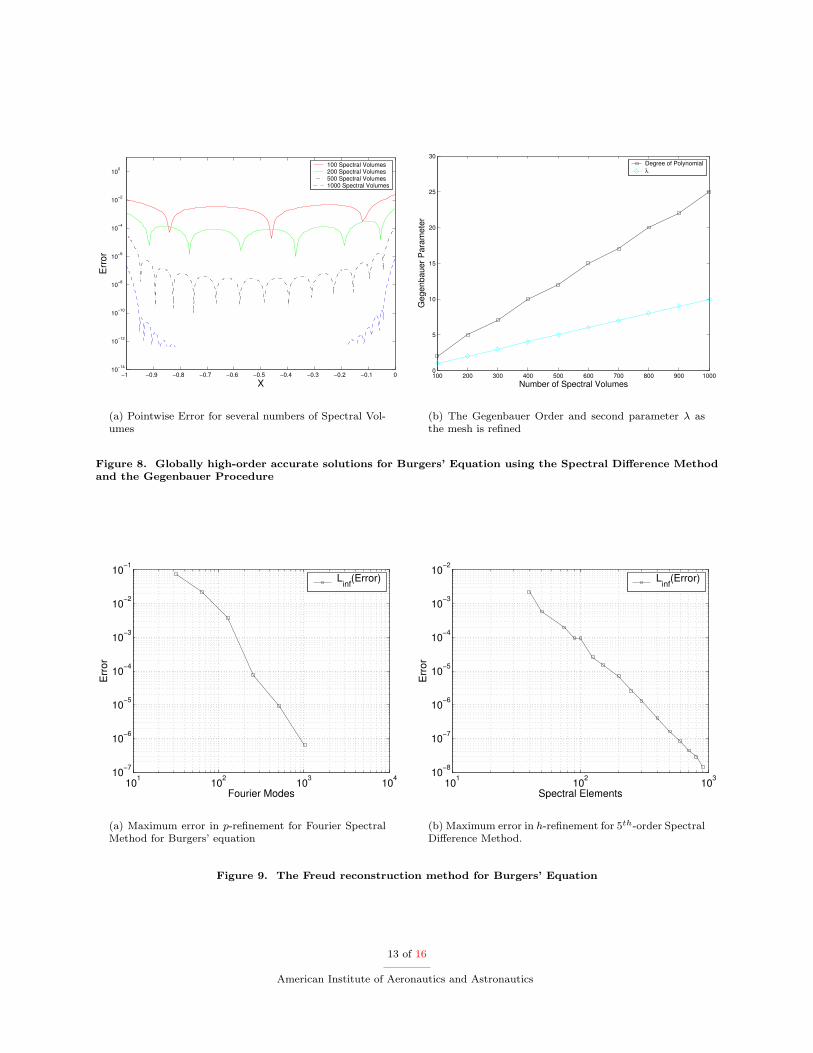
volumes after reprojection of the solution onto Gegenbauer polynomials. The effectiveness of the procedureis demonstrated by figure 7, where a comparison of the original numerical solution with the expansion inGegenbauer polynomials is shown. A grid refinement study to verify the nominal order of accuracy as Nis increased has been carried out, and is shown in figure 6(b) together with a reference slope indicatingthe required reduction in global error measures for the nominal fifth order of accuracy. It can be seen thatwhile the original solution fails to converge in maximum norm, and the L2 norm of the Error barely reachesfirst order, the re-projected solution converges in both L2 and maximum norm. It should be emphasizedthat error norms were computed using all nodes in the mesh, so that all global error measures include thediscontinuity. The slope of the errors, however, is not constant, which can be explained by the fact that theparameters of the Gegenbauer polynomials, i.e. the order and second parameter λ, have to be adjusted as themesh is refined. In theory one ought to make the number of Gegenbauer modes proportional to the number oforiginal spectral modes. These, however, remain constant here, because the order of approximation is fixed,i.e. we are carrying out h-refinement instead of p-refinement. It seems most fitting to make the parametersproportional to the total number of collocation nodes. The dependence of the parameters as a function of thenumber of spectral volumes is depicted in figure 8(b) on page 13. It should be pointed out at this point that

11 of 16


−1 −0.8 −0.6 −0.4 −0.2 0 0.2 0.4 0.6 0.8 10.4

0.6

0.8

1

1.2

1.4

1.6

1.8

2

X

U

No PostprocessingGegenbauer Procedure

(a) Solution using the Spectral Difference Method with200 Spectral Elements with and without Gegenbauerpostprocessing

(b) Close-up view of the solution near the discontinuitywith and without the Gegenbauer procedure


the parameters are not optimized in any way, but merely represent “best practice” values. Some suggestionsregarding their optimization have been made in the literature.17

Figure 8(a) on the following page shows the pointwise errors for the smooth subdomain −1 ≤ x ≤ 0. Itcan be seen that the error decreases according to the nominal order of accuracy up to the endpoints of thedomain, the right endpoint being the discontinuity at x = 0.

A further reduction of the maximum error, i.e. below roughly 1. · 10−8 could not be achieved, due tothe inherent numerical problems mentioned in section III. In fact, if the mesh is further refined the errorincreases and diverges in the limit N → ∞ if the Gegenbauer parameters are further increased, althoughthis can be prevented if the parameters are frozen. For the case of 1000 spectral volumes the order of thepolynomials is m = 25 and λ = 10. The value of the corresponding Gegenbauer polynomial at x = 1 isC10

25 (1) = 1.4 ·10+12 . Further refinement increases these numbers, and it becomes clear how it is increasinglydifficult to achieve an absolute precision of at least twenty orders of magnitude below the computed valuesof the Gegenbauer polynomials.

No limiters have been used for these computations, which means that we have relied solely on thedissipation from the fluxes at element boundaries to stabilize the solution. This approach, while acceptablefor low-order of accuracy must necessarily fail for p-refinement, i.e. as the degree of spectral approximation isincreased. We show below that alternatively a spectral adaptive filtering procedure can be used to stabilizethe solution.

As an alternative to Gegenbauer polynomials the Freud polynomials can be used to perform Gibbs-complementary reconstruction. We have carried out two tests for the Burgers’ equation. Firstly we solve theequations by a Fourier spectral method using a straight spectral differentiation along with an exponentialfilter to stabilize the solution. Secondly we use the 5th order Spectral Difference method. These twoapproaches allow us to test the Freud reconstruction procedure in p-refinement and h-refinement. Theresults of the refinement studies are shown in figure 9 on the next page. While the maximum errors canbe reduced to about the same level as for the Gegenbauer reconstruction method, the numerical behavior isgenerally more benign for the Freud reconstruction.

12 of 16


−1 −0.9 −0.8 −0.7 −0.6 −0.5 −0.4 −0.3 −0.2 −0.1 010−14

10−12

10−10

10−8

10−6

10−4

10−2

100

X

Err

or

100 Spectral Volumes200 Spectral Volumes500 Spectral Volumes1000 Spectral Volumes

(a) Pointwise Error for several numbers of Spectral Vol-umes

100 200 300 400 500 600 700 800 900 10000

5

10

15

20

25

30

Number of Spectral Volumes

Geg

enba

uer P

aram

eter

Degree of Polynomialλ

(b) The Gegenbauer Order and second parameter λ asthe mesh is refined


101

102

103

10410

−7

10−6

10−5

10−4

10−3

10−2

10−1

Fourier Modes

Err

or

Linf

(Error)

(a) Maximum error in p-refinement for Fourier SpectralMethod for Burgers’ equation

101

102

10310

−8

10−7

10−6

10−5

10−4

10−3

10−2

Spectral Elements

Err

or

Linf

(Error)

(b) Maximum error in h-refinement for 5th-order SpectralDifference Method.

Figure 9. The Freud reconstruction method for Burgers’ Equation

13 of 16


As a preliminary testcase for the Euler equations the Sod shocktube problem has been considered. Fig-ure 10 shows the solution obtained with a fourth-order spectral difference method with scalar diffusion at

0 0.1 0.2 0.3 0.4 0.5 0.6 0.7 0.8 0.9 10.1

0.2

0.3

0.4

0.5

0.6

0.7

0.8

0.9

1Sod Shocktube Test Case

x

ρ

Spectral DifferenceExact

(a) Density

0 0.1 0.2 0.3 0.4 0.5 0.6 0.7 0.8 0.9 1−0.2

0

0.2

0.4

0.6

0.8

1

Sod Shocktube Test Case

xU

Spectral DifferenceExact

(b) Velocity

Figure 10. Solution for the Sod shocktube case using 800 Elements

element boundaries, along with Butcher-Runge-Kutta time integration. It can be seen from the figure thatthe shocks and the contact discontinuity are perfectly captured. No limiter or spectral diffusion has beenused, which means that the dissipation from the element boundaries must suffice to stabilize the solution.This might be the reason that the maximum error, e.g. in density, could not be reduced beyond approx-imately L∞(ρ − ρexact) ≈ 1 · 10−3 . However, note that this level of error represents the maximum errorin the domain, including the discontinuities. The best way to stabilize the scheme will be the subject offurther research. To demonstrate the effect of the reconstruction we show the unprocessed solution alongwith the reprojected one in figure 11 on the next page. The unlimited original solution, computed by the4th order spectral difference method, exhibits oscillations of the order of what one would expect from Gibb’sphenomenon, if the analytical solution were to be expanded in smooth basis functions.

Naturally, the Spectral Difference method can also be used with conventional limiting functions. Whilethis reduces the accuracy near discontinuities such concepts are comparatively well established and under-stood. Figure 12(a) shows the solution for quasi-1D nozzle flow with a shock in terms of the density, computedwith a 4th order Spectral Difference method and a minmod limiter. Good shock capturing capabilities canbe observed. Figure 12(b) shows the Entropy error for the 3rd order and 4th order schemes. While theentropy behind the shock is constant, fixed by the shock jump conditions, the entropy in front of the shockshould decrease with increasing accuracy. Indeed it does so, with slight spikes visible at the nozzle throat.This is due to the fact that a TVD (total variation diminishing) limiter has been used, which is active atsmooth extrema. This could be removed by using a total variation bounded version of the limiter (TVB).This is planned for future work.

V. Conclusion and Future Work

First steps toward high-order accurate solutions for conservation laws with discontinuous solutions havebeen shown. The extension to higher dimensions will be a focus of research. So far only the spectral difference

14 of 16


(a) Density (b) Velocity

Figure 11. Solution for the Sod shocktube case using 800 Elements.

(a) Density distribution for the 4th order Spectral Dif-ference Scheme and 40 elements.

(b) Entropy Error for the 3rd and 4th order scheme with40 elements.

Figure 12. Solution for nozzle flow with a shock using the Spectral Difference method with a minmod limiter.

15 of 16


method has been used, but we will also consider spectral methods. The nature of the Gibbs-complementaryreconstruction seems to be well suited for use with spectral and multidomain spectral methods. The extensionto viscous fluid flow is another important issue that will be considered in the future.

VI. Acknowledgements

This work has been supported in part by Stanford University through a Stanford Graduate Fellowship(SGF).

References

1Liu, Y., Vinokur, M., and Wang, Z. J., “Discontinuous spectral difference method for conservation laws on unstructuredgrids,” Proceedings of the 3rd International Conference on Computational Fluid Dynamics, July 12-16, 2004, Toronto, Canada,Springer, 2004.

2Wang, Z. J. and Liu., Y., “The Spectral Difference Method for the 2D Euler Equations on Unstructured Grids,” Aiaapaper 2005-5112, 2005.

3Kopriva, D. A., “A Conservative Staggered-Gri Chebyshev Multidomain Method for Compressible Flows II: Semi-Structured Method,” J. Comp. Phys.., Vol. 128, 1996, pp. 475.

4Hesthaven, J. S., “From Electrostatics to Almost Optimal Nodal Sets for Polynomial Interpolation in a Simplex,” SIAMJ. Num. Anal., Vol. 35, No. 2, 1998, pp. 655–676.

5Jameson, A., “Analysis and design of numerical schemes for gas dynamcics 2: Artificial diffusion and discrete shockstructure,” Int. J. Comp. Fluid. Dyn., Vol. 5, 1995, pp. 1–38.

6Cockburn, B. and Shu, C. W., “TVB Runge-Kutta Local Projection Discontinuous Galerkin Finite Element Method forConsrvation Laws II: General Framework,” Math. Comp., Vol. 52, No. 186, 1988, pp. 411–435.

7Tadmor, E., “Convergence of Spectral Methods for Nonlinear Consrvation Laws,” SIAM J. Num. Anal., Vol. 26, No. 1,1989, pp. 30–44.

8Gottlieb, D. and Hesthaven, J. S., “Spectral Methods for Hyperbolic Problems,” J. Comp. Appl. Math, Vol. 128, 2001,pp. 83–131.

9Gottlieb, D. and Orszag, S. A., Numerical Analysis of Spectral Methods: Theory and Applications, CBMS-NSF RegionalConference Series in Applied Mathematics, 1977.

10Gottlieb, D. and Shu, C. W., “On the Gibbs Phenomenon V: Recovering exponential accuracy from collcoation pointvalues of a piecwise analytic function,” Numer. Math., Vol. 71, 1995, pp. 511–526.

11Gottlieb, D. and Shu, C. W., “On the Gibbs Phenomenon and its Resolution,” SIAM Rev., Vol. 39, No. 4, 1997, pp. 644–668.

12Bateman, H., Higher Transcendental Function, Vol 2 , McGraw Hill, 1953.13Tanner, J. and Gelb, A., “Robust reprojection methods for the resolution of Gibbs phenomenon,” Appl. Comput. Harm.

Anal. (preprint), 2004.14Gelb, A., “Detection of Edges in Spectral Data,” Appl. Comp. Harm. Anal., Vol. 7, 1999, pp. 101–135.15Gelb, A. and Tadmor, E., “Detection of Edges in Spectral Data II. Nonlinear Enhancement,” SIAM J. Numer. Anal.,

Vol. 38, No. 4, 2000, pp. 1389–1408.16Bhatnagar, P., Gross, E., and Krook, M., “A model for collision processes in gases I: Small amplitude processes in charged

and neutral one-component systems,” Phys. Rev., Vol. 94, 1954, pp. 511.17Gelb, A., “Parameter Optimization and Reduction of Round-Off Error for the Gegenbauer Reconstruction Method,” J.

Sci. Comp., Vol. 20, No. 3, 2004, pp. 433–459.

16 of 16


Documents

High-Order Accurate Methods for High-Speed Flowaero-comlab.stanford.edu/Papers/may.aiaa.05-5251.pdf · High-Order Accurate Methods for High-Speed Flow Georg May∗ and Antony Jameson†