HIGH GRADE CONTROL OF LINEAR INDUCTION MOTOR DRIVES …

HIGH GRADE CONTROL OF LINEAR INDUCTION MOTOR DRIVES

by

HAIDONG YU

Presented to the Faculty of the Graduate School of

The University of Texas at Arlington in Partial Fulfillment

of the Requirements

for the Degree of

DOCTOR OF PHILOSOPHY

THE UNIVERSITY OF TEXAS AT ARLINGTON

December 2007

Copyright © by HAIDONG YU 2007

All Rights Reserved

iii

ACKNOWLEDGEMENTS

I am sincerely grateful to my supervisor Dr. Babak Fahimi for his supervision

and support. His guidance and encouragement has been vital to my learning. I thank

him for mentoring me for completion of this dissertation.

I would like to thank Dr. Raymond R. Shoults, Dr. Wei-Jen Lee, Dr. Kai-Sing

Yeung, and Dr. Soontorn Oraintara for being in my supervising committee. Their views

and suggestions have been valuable for completeness of the dissertation.

I wish to thank all the members from the Power Electronics and Controlled

Motion (PECM) Laboratory for the support in completion of this dissertation.

I also want to thank Dr. Steven D. Pekarek and Mr. Dezheng Wu from Purdue

University for their cooperation with PECM lab.

Last but not least, my thanks are extended to my parents for their inexhaustible

love and support to me. I also want to express my appreciation to Helen Huang for her

encouragement and support.

November 14, 2007

iv

ABSTRACT

HIGH GRADE CONTROL OF LINEAR INDUCTION MOTOR DRIVES

Publication No. ______

HAIDONG YU, PhD.

The University of Texas at Arlington, 2007

Supervising Professor: Babak Fahimi

Linear induction machines (LIM) have been widely utilized in military,

transportation, and aerospace due to the impressive advantages such as simple

configuration, easy maintenance, and high acceleration/deceleration. However, the

existence of trailing eddy current effects and magnetic asymmetry effects undermines

the expected functionality of vector control even though LIM possesses similarities

from its rotary counterpart. As a result, it has been a focal research area to either

improve the performance of vector control for LIM or develop a new high grade control

strategy.

v

Therefore, the in-depth exploration of electromagnetic behavior of LIM has

been a fundamental step for investigation of LIM. From both finite element analysis

(FEA) and experiment, it is verified that the two open ends in the primary of LIM result

in the magnetic asymmetry effects. Furthermore, both the trailing eddy current effects

and magnetic asymmetry effects cause non-sinusoidal magneto-motive force (MMF).

This undermines the basic assumption of vector control that the fundamental MMF

should be sinusoidal. Moreover, FEA is a good tool for numerical-based analysis of

electrical machines. However, the computational effort is extremely intensive.

Therefore, the field reconstruction method (FRM) for LIM is proposed in this

dissertation. FRM significantly reduces the computational time, but supplies steady

state calculation in good accuracy. This dissertation also proposes a maximum

force/ampere control, which has impressive advantages such as simple implementation,

easy controllability, and maximum energy conversion ratio. The maximum

force/ampere control is validated by both simulation results and experimental

verification.

The contribution of this dissertation can be summarized as follows:

1. Systematic exploration of electromagnetic behavior of LIM;

2. Development of field reconstruction method for LIM;

3. Invention and implementation of maximum force/ampere control.

vi

TABLE OF CONTENTS

ACKNOWLEDGEMENTS....................................................................................... iii ABSTRACT .............................................................................................................. iv LIST OF ILLUSTRATIONS..................................................................................... ix Chapter 1. INTRODUCTION......................................................................................... 1 1.1 Background and Significance................................................................... 1 1.2 Motivation and Technical Objectives....................................................... 4 1.3 Contributions........................................................................................... 5 2. ELECTROMAGNETIC BEHAVIOR OF LINEAR INDUCTION MACHINES................................................................................................... 6 2.1 LIM Model in FEA.................................................................................. 6 2.2 Trailing Eddy Current Effects.................................................................. 8 2.3 Magnetic Asymmetry Effects.................................................................. 8 2.3.1 Experimental Verification of Magnetic Asymmetry Effects.... 12 2.3.2 Magnetic Asymmetry Effects on Force Characteristics of LIM.................................................... 17 2.3.3 Magnetic Asymmetry Effects on IFOC of LIM ....................... 18 2.3.4 Investigation on Magnetic Asymmetry Effects on IFOC of LIM from a Magnetic Perspective ............................. 21 2.4 Airgap Length Effect............................................................................... 24

vii

2.5 Secondary Electric Conductivity’s Effect............................................... 28 2.6 Back EMF Characteristics....................................................................... 30 3. FIELD RECONSTRUCTION METHOD OF LINEAR INDUCTION MACHINES................................................................................................... 34 3.1 Background.............................................................................................. 34 3.2 Basis Function Identification................................................................... 36 3.2.1 Primary Basis Function Derivation .......................................... 36 3.2.2 Secondary Basis Function Derivation ...................................... 38 3.3 Field Reconstruction................................................................................ 41 3.4 Verification of Field Reconstruction........................................................ 42 3.5 Saturation Effects...................................................................................... 46

4. INDIRECT FIELD ORIENTED CONTROL OF LINEAR INDUCTION MACHINES................................................................................................... 49 4.1 Fundamentals of IFOC ............................................................................ 50 4.1.1 Identification of Secondary Time Constant.............................. 51 4.1.2 Determination of Parameters in dq Axis .................................. 52 4.2 Closed Loop Speed Control Using IFOC ................................................ 53 4.2.1 Simulation Study of IFOC........................................................ 53 4.2.2 Experimental Verification of IFOC.......................................... 55

5. MAXIMUM FORCE PER AMPERE CONTROL OF LINEAR INDUCTION MACHINES............................................................ 62 5.1 Principles of Maximum Force per Ampere Control ................................ 62 5.2 Simulation Study of Maximum Force per Ampere Control .................... 65 5.3 Experimental Verification of Maximum Force per Ampere Control ...... 72

viii

5.4 Comparison between IFOC and Maximum Force per Ampere Control ..................................................... 77

6. CONCLUSIONS AND FUTURE RESEARCH............................................ 81 Appendix A. SPECIFICATIONS OF LIM......................................................................... 83 B. LIM DRIVE SYSTEM ................................................................................. 85 REFERENCES .......................................................................................................... 87 BIOGRAPHICAL INFORMATION......................................................................... 90

ix

LIST OF ILLUSTRATIONS

Figure Page 1 Imaginary Process of Obtaining Linear Electric Machines.................................... 1 2 Classification of Linear Electric Machines............................................................. 2 3 Air Train (From Wikipedia).................................................................................... 3 4 Nagahori Tsurumi-ryokuchi Line in Japan (From Wikipedia) ............................... 3 5 Cross Sectional View of LIM under Investigation ................................................. 6 6 Primary Winding Scheme ....................................................................................... 7 7 Initial 2D Mesh of LIM in FEA.............................................................................. 7 8 Trailing Eddy Current in FEA ................................................................................ 8 9 Flux Density Distribution when Phase a is Excited by a DC Current .................... 9

10 Flux Density Distribution when Phase b is Excited by a DC Current .................... 9

11 Flux Density Distribution when Phase c is Excited by a DC Current .................... 9

12 Excitation Circuit of Direct Method ....................................................................... 10

13 Normal Flux Density in the Middle of Airgap when Phase a is Excited by a DC Current ........................................................................ 11

14 Normal Flux Density in the Middle of Airgap when

Phase b is Excited by a DC Current ........................................................................ 11

15 Normal Flux Density in the Middle of Airgap when Phase c is Excited by a DC Current ........................................................................ 12

16 Indirect Excitation Method ..................................................................................... 13

17 Normal Flux Density of Three Connections in FEA .............................................. 13

x

18 Normal Flux Density of Three Connections from Experimental Testbed.............. 14

19 Prototype of LIM under Investigation .................................................................... 14

20 Flux Linkage of Phase a under a Set of Three Phase Balanced Sinusoidal Current Sources Excitation ............................... 16

21 Flux Linkage of Phase b under a Set of

Three Phase Balanced Sinusoidal Current Sources Excitation ............................... 16

22 Flux Linkage of Phase c under a Set of Three Phase Balanced Sinusoidal Current Sources Excitation ............................... 17

23 Average Force Variations with Respect to

Frequency at Linear Speed of 5 m/sec .................................................................... 18

24 Block Diagram of IFOC Functionality ................................................................... 19

25 Average Thrust Variation with Respect to Iq when Id is Fixed at 1 A................... 20

26 Average Normal Force Variation with Respect to Iq when Id is Fixed at 1 A....... 20

27 Magnetization Curve of Primary with Respect to Iq .............................................. 22

28 Magnetization Curve of Primary with Respect to Id .............................................. 22

29 Magnetization Curve of Secondary with Respect to Iq .......................................... 23

30 Magnetization Curve of Secondary with Respect to Id .......................................... 23

31 Force Variations with Respect to Airgap Length under Motoring Condition (1 m/sec)................................................................................. 25

32 Force Variations with Respect to Airgap Length under

Electromagnetic Braking Condition (1 m/sec)........................................................ 26

33 Force Variations with Respect to Airgap Length under Motoring Condition (10 m/sec)............................................................................... 26

34 Force Variations with Respect to Airgap Length under

Generating Condition (10 m/sec) ............................................................................ 27

35 Force Variations with Respect to Airgap Length under Motoring Condition (15 m/sec)............................................................................... 27

xi

36 Force Variations with Respect to Airgap Length under Generating Condition (15 m/sec) ............................................................................ 28

37 Force Variation with Secondary Electric Conductivity at

Linear Speed 1 m/sec .............................................................................................. 29

38 Force Variation with Secondary Electric Conductivity at Linear Speed 15 m/sec ............................................................................................ 30

39 Back EMF Amplitude Variation with Frequency at 1 m/sec.................................. 31

40 Back EMF Amplitude Variation with Frequency at 5 m/sec.................................. 32

41 Phase Shift between Back EMF and Phase Current at 1 m/sec .............................. 32

42 Phase Shift between Back EMF and Phase Current at 5 m/sec .............................. 33

43 Positive Directions of Normal and Tangential Components .................................. 35

44 Tangential Basis Functions of Three Phases .......................................................... 37

45 Normal Basis Functions of Three Phases ............................................................... 38

46 Two Step Procedure of Basis Function Identification ............................................ 40

47 Field Reconstruction Procedure.............................................................................. 41

48 Tangential Flux Density.......................................................................................... 43

49 Normal Flux Density............................................................................................... 43

50 Normal Flux Density in the Middle of Airgap at One Particular Position Using FRM........................................................................ 44

51 Normal Flux Density in the Middle of Airgap at the

Same Position with Figure 50 from Experiment (0.05 T/Div)................................ 44

52 Thrust Variations of Three Methods....................................................................... 45

53 Normal Force Variations of Three Methods........................................................... 46

54 Tangential Flux Density with Saturation ................................................................ 47

55 Normal Flux Density with Saturation ..................................................................... 47

xii

56 Thrust Variations of Three Methods with Saturation ............................................. 48

57 Normal Force Variations of Three Methods with Saturation ................................. 48

58 Measurement of Secondary Time Constant (Vertical Axis: Voltage, Horizontal Axis: Time).................................................... 52

59 Block Diagram of Closed Loop Speed Control with IFOC.................................... 54

60 Speed Response of IFOC in Simulation ................................................................. 55

61 Block Diagram of Hardware Set Up....................................................................... 56

62 Speed Response of IFOC from Experiment (No Load).......................................... 57

63 Phase Starting Current of IFOC (No Load) ............................................................ 57

64 Transition of Operation Mode of Phase Current in IFOC (No Load)..................... 58

65 Phase Braking Current of IFOC (No Load)............................................................ 58

66 Speed Response of IFOC from Experiment (22 lbs Load) ..................................... 60

67 Phase Starting Current of IFOC (22 lbs Load) ....................................................... 60

68 Transition of Operation Mode of Phase Current in IFOC (22 lbs Load)................ 61

69 Phase Braking Current of IFOC (22 lbs Load) ....................................................... 61

70 Average Thrust Variation with Excitation Frequency at Different Linear Speeds ................................................... 64

71 Average Normal Force Variation with

Excitation Frequency at Different Linear Speeds ................................................... 64

72 Control Block Diagram for the Maximum Force/Ampere Control ........................ 65

73 Speed Response of Maximum Force/Ampere Control ........................................... 66

74 Profile of Optimum Excitation Frequency.............................................................. 66

75 Simulated Reference Phase Current and Predicted Phase Current ......................... 67

76 Zoomed Phase Current Profile................................................................................ 67

xiii

77 Thrust Ripple Percentage with Respect to Frequency at Linear Speed 5 m/sec .............................................................................................. 68

78 Normal Force Ripple Percentage with Respect to Frequency at

Linear Speed 5 m/sec .............................................................................................. 69

79 Thrust Variations with Excitation Frequency for Two Airgap Lengths when Linear Speed is 10 m/sec............................................. 70

80 Normal Force Variations with Excitation Frequency for

Two Airgap Lengths when Linear Speed is 10 m/sec............................................. 71

81 Thrust Variations with Excitation Frequency for Two Secondary Electric Conductivity Values ........................................................ 71

82 Normal Force Variations with Excitation Frequency for

Two Secondary Electric Conductivity Values ........................................................ 72

83 Speed Response of Maximum Force/Ampere Control (No Load) ......................... 73

84 Transition Phase Current from Starting to Steady State (No Load) ....................... 73

85 Transition Phase Current from Steady State to Braking (No Load) ....................... 74

86 Zoomed Steady State Phase Current Using Maximum Force/Ampere Control (No Load)............................................... 74

87 Speed Response of Maximum Force/Ampere Control (22 lbs Load)..................... 75

88 Transition Phase Current from Starting to Steady State (22 lbs Load)................... 76

89 Transition Phase Current from Steady State to Braking (22 lbs Load) .................. 76

90 Zoomed Steady State Phase Current Using Maximum Force/Ampere Control (22 lbs Load).......................................... 77

91 Speed Response of Both Methods (No Load)......................................................... 78

92 Speed Response of Both Methods (22 lbs Load).................................................... 79

93 Speed Profile Subject to a Sudden Change of Load (22 lbs) Using IFOC ............. 79

94 Speed Profile Subject to a Sudden Change of Load (22 lbs) Using Maximum Force/Ampere Control ................................................................ 80

1

CHAPTER 1

INTRODUCTION

1.1 Background and Significance

The origin of linear electric machines can be traced back about one century ago.

However, only after 1960, due to the occurrence of the modern power electronics

technique, linear electric machines have attracted a great deal of interest. Linear electric

machines can be conceptually realized by “cutting” and “unrolling” their counterpart,

rotary electric machines. The process is illustrated by figure 1.

Figure 1 Imaginary Process of Obtaining Linear Electric Machines

From the aspect of electrical excitation, linear electric machines include linear

dc machines, linear synchronous machines, linear induction machines, and linear step

motors. With respect to geometry, linear electric machines have flat and tubular types.

2

The whole family of linear electric machines is classified in figure 2.

Linear Electric Machines

Linear Flat Machine

Geometry

Tubular Linear Electric Machine

Single Sided

Double Sided

Linear DC Machine

Linear Synchronous

Machine

Linear Induction Machine

Linear Step Motor

Electrical Synchronous

Permanent Synchronous Reluctance

Excitation

Figure 2 Classification of Linear Electric Machines

As one category of linear electric machines, linear induction machines (LIM)

have been utilized in a wide range of applications [1]-[6] such as military,

transportation, and aero space to name a few due to the impressive advantages such as

simple configuration, easy maintenance, high propulsion, and no need for the

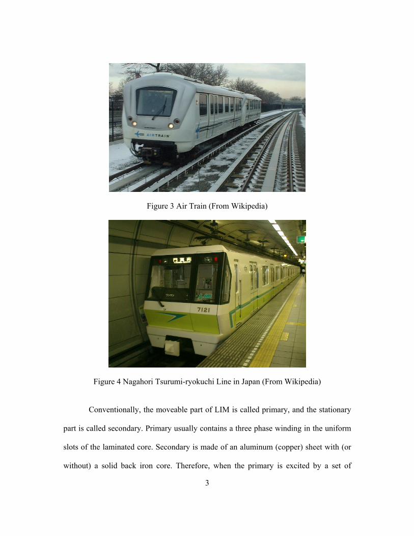
transformation systems from rotary to translational movement. Figure 3 and 4 illustrate

applications mentioned above. This dissertation will investigate single sided linear flat

induction machine.

3

Figure 3 Air Train (From Wikipedia)

Figure 4 Nagahori Tsurumi-ryokuchi Line in Japan (From Wikipedia)

Conventionally, the moveable part of LIM is called primary, and the stationary

part is called secondary. Primary usually contains a three phase winding in the uniform

slots of the laminated core. Secondary is made of an aluminum (copper) sheet with (or

without) a solid back iron core. Therefore, when the primary is excited by a set of

4

balanced sinusoidal currents, there will be eddy current inducing on the secondary

aluminum sheet. These two electromagnetic sources will react to produce

electromagnetic forces. The tangential force is called thrust. The other component of

force is called normal force.

1.2 Motivation and Technical Objectives

There are three most popular control strategies for linear induction motor drives.

They are scalar control (V/F) [7] and [8], direct torque control (DTC) [9], and vector

control [10]-[12]. Scalar control is also called Volt/Hertz control. It regulates the ratio

of voltage with frequency at a constant value. Direct torque control uses errors between

the references of primary flux and the force with their estimated values to determine the

optimal switching configuration of the three phase inverter every sample time. Vector

control includes direct field oriented control (DFOC) [11] and indirect field oriented

control (IFOC) [13]. Vector control measures or estimates the location of rotor flux

axis, and uses the flux angle to decouple the stator currents into quadrature and direct

components, i.e. qI and dI . dI is normally regulated at its rated value, and qI is

regulated to deliver commanded force. Since this family of machines possesses

similarities with their rotary counterparts, vector control scheme is the most often used

technique for LIM, and has been considered as the best control solution for LIM. Some

other control strategies [13]-[15] based on vector control incorporate advanced control

methods to improve the performance of LIM.

However, some electromagnetic behavior of LIM such as trailing eddy current

effects [16]-[19] and magnetic asymmetry effects [20] and [21] can undermine the

5

expected functionality of vector control. As a result, one can not harvest the high grade

control performance from LIM using vector control. Therefore, the motivation of this

dissertation is to develop and implement a high grade control scheme for LIM to

achieve simple implementation, fast response, and maximum energy conversion ratio.

Furthermore, the new invented control scheme, maximum force/ampere control, will be

compared with the conventional IFOC both in simulation study and experimental test to

illustrate its superior performance.

Development and implementation of a high grade control strategy for LIM has

led to exploration of the complete understanding of electromagnetic behavior of LIM.

In addition, finite element analysis (FEA) [22]-[25] is a widely used tool for numerical-

based analysis of electrical machines. However, FEA requires intensive computational

effort, which is not time efficient. Therefore, a new efficient field calculation technique,

field reconstruction method (FRM) [26] and [27], is proposed to ease the investigation

of LIM.

1.3 Contributions

The contributions of this dissertation can be summarized as:

1. Systematic exploration of electromagnetic behavior of LIM and discovery

of shortcomings of vector control method in optimal control of LIM;

2. Development of field reconstruction method for LIM;

3. Invention and implementation of maximum force/ampere control.

6

CHAPTER 2

ELECTROMAGNETIC BEHAVIOR OF LINEAR INDUCTION MACHINES

In order to develop and implement a high grade control scheme for linear

induction machine, in-depth knowledge of electromagnetic behavior is necessary. Finite

element analysis (FEA) is used in this procedure.

2.1 LIM Model in FEA

Figure 5 shows the cross sectional view of the prototype in FEA based on the

machine construction details. Commercially available package MagNet from Infolytica

is used for this investigation. The primary winding scheme is shown in figure 6. The

type of the winding is in ‘Star’ or ‘Y’ connection.

Figure 5 Cross Sectional View of LIM under Investigation

7

Figure 6 Primary Winding Scheme

Figure 7 illustrates the initial 2D mesh of LIM under investigation. The solver

method in FEA is Newton-Raphson iteration method. The maximum iteration number is

20, and the polynomial order is 1. In order to guarantee the accuracy of FEA

calculations, the maximum length of triangle sides located around the airgap, aluminum

sheet surface, and primary teeth surface is about 1 mm.

Figure 7 Initial 2D Mesh of LIM in FEA

8

2.2 Trailing Eddy Current Effects

As shown in figure 8, when linear induction machines move forward (from left

to right), there is always eddy current that is not in the overlapped region between

primary and secondary. This eddy current is called trailing eddy current. Trailing eddy

current can cause non-sinusoidal and asymmetric magneto-motive force (MMF). These

effects will undermine the proper functionality of conventional vector control of LIM.

Figure 8 Trailing Eddy Current in FEA

2.3 Magnetic Asymmetry Effects

Unlike rotary induction machine, LIM has two open ends in primary. Due to

different relative positions of phases a, b, and c in primary, the contribution of each

phase to the MMF will be unequal. Figure 9, 10, and 11 illustrate the flux density

distribution when phases a, b, and c are excited by a dc current respectively under lock

up condition (direct method). The excitation circuit is shown in figure 12. One can

notice that the peak flux densities in the primary in each case are 0.560416 T, 0.507523

T, and 0.582781 T in sequence. There is a significant difference in primary flux density

between phase b, and phases a and c.

9

Figure 9 Flux Density Distribution when Phase a is Excited by a DC Current

Figure 10 Flux Density Distribution when Phase b is Excited by a DC Current

Figure 11 Flux Density Distribution when Phase c is Excited by a DC Current

10

Coil_phase_A

T1 T2

Coi l_phase_B

T1 T2

Coi l_phase_C

T1 T2

Ia

SIN

Figure 12 Excitation Circuit of Direct Method

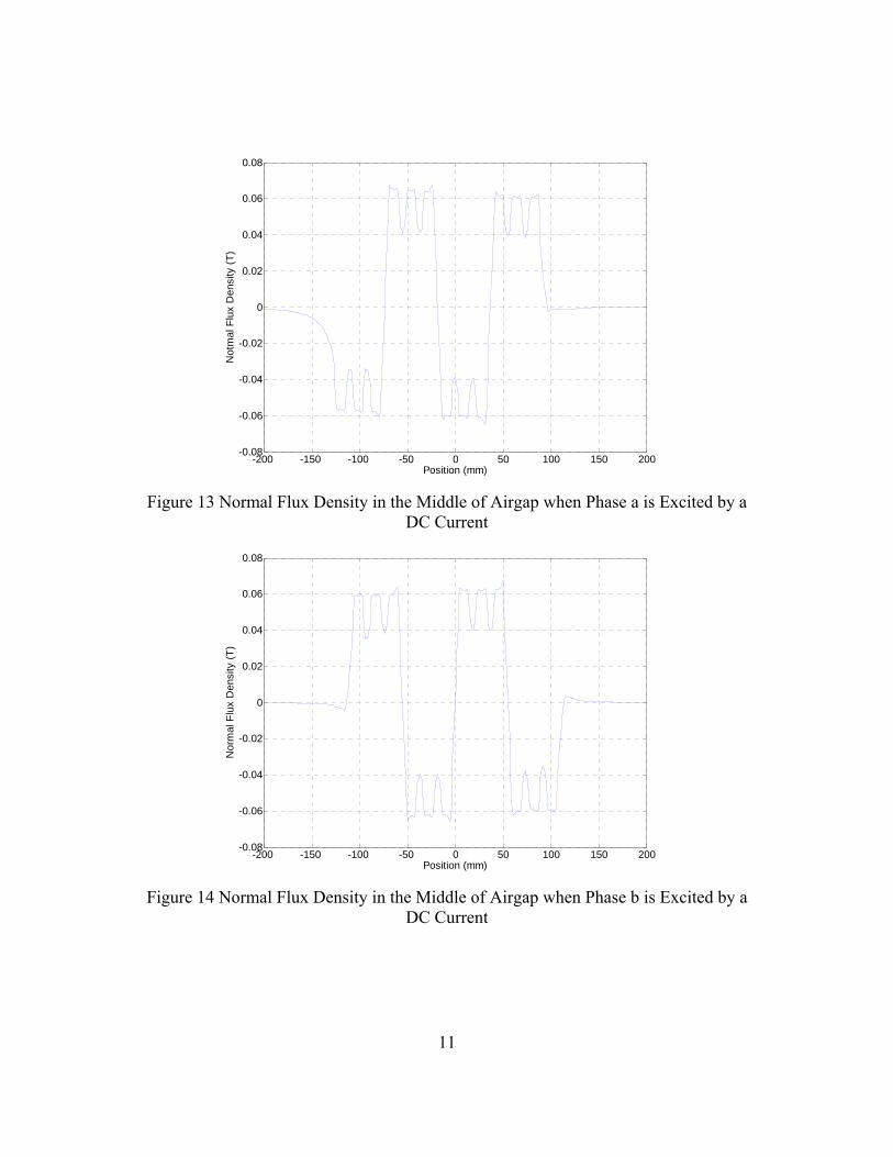
Figure 13, 14, and 15 display the normal flux density in the middle of airgap

when phases a, b, and c are excited by a dc current respectively. One can notice the

waveform of phase a is the mirror image of the waveform of phase c. However, the

waveform of phase b is antisymetric itself. This observation verifies that the structure of

two open ends on the primary contributes to the magnetic asymmetry effects of LIM.

11

-200 -150 -100 -50 0 50 100 150 200-0.08

-0.06

-0.04

-0.02

0

0.02

0.04

0.06

0.08

Position (mm)

Not

mal

Flu

x D

ensi

ty (T

)

Figure 13 Normal Flux Density in the Middle of Airgap when Phase a is Excited by a

DC Current

-200 -150 -100 -50 0 50 100 150 200-0.08

-0.06

-0.04

-0.02

0

0.02

0.04

0.06

0.08

Position (mm)

Nor

mal

Flu

x D

ensi

ty (T

)

Figure 14 Normal Flux Density in the Middle of Airgap when Phase b is Excited by a

DC Current

12

-200 -150 -100 -50 0 50 100 150 200-0.08

-0.06

-0.04

-0.02

0

0.02

0.04

0.06

0.08

Position (mm)

Nor

mal

Flu

x D

ensi

ty (T

)

Figure 15 Normal Flux Density in the Middle of Airgap when Phase c is Excited by a

DC Current

2.3.1 Experimental Verification of Magnetic Asymmetry Effects

Since the winding connection of primary is ‘Y’ connection without access to the

neutral point, in order to implement experiments, the circuit shown in figure 16 (indirect

method) has been used. In the indirect method, when one phase is excited by a dc

current, the other two phases are connected in parallel to supply the return path for the

first phase current. As a result, when phase a is excited and phase b and c are connected

in parallel, this condition is defined as A-BC. Based on the above method, figure 17

shows the normal airgap flux density of three connections in FEA.

13

Coil_phase_A

T1 T2

Coi l_phase_B

T1 T2

Coi l_phase_C

T1 T2

Ia

SIN

Figure 16 Indirect Excitation Method

0 5 10 15 20 25-0.5

-0.4

-0.3

-0.2

-0.1

0

0.1

0.2

0.3

0.4

0.5

Position (cm)

Flux

Den

sity

(kG

)

A-BCB-CAC-AB

Figure 17 Normal Flux Density of Three Connections in FEA

14

0 5 10 15 20 25-0.5

-0.4

-0.3

-0.2

-0.1

0

0.1

0.2

0.3

0.4

0.5

Position (cm)

Flux

Den

sity

(kG

)

A-BCB-CAC-AB

Figure 18 Normal Flux Density of Three Connections from Experimental Testbed

Figure 19 Prototype of LIM under Investigation

15

Figure 18 shows normal flux density of three connections of the experimental

LIM testbed shown in figure 19. Figure 19 illustrates a single sided, three phase, 4 pole

linear induction machine being investigated in this dissertation. In figure 19, the blue

part in the middle of railway is primary, and beneath that is the aluminum sheet backed

with iron core. Detailed information is given in APPENDIX A. Comparing figure 18

with figure 17, one can observe a close match between the two figures. In addition, it is

shown that the waveform of excitation connection A-BC is mirror image to that of

excitation connection C-AB. However, the waveform of excitation caused by B-CA

connection is antisymetric itself. These observations are similar with the results from

the direct method. Therefore, different relative positions of a, b, and c phases in primary

result in the magnetic asymmetry effects.

From [28], for conventional rotary induction machines, the following equation

holds:

)cos( ses tKMMF φω −= (1)

However, for LIM, due to the asymmetry between contributions of the primary phases,

the above equation will not hold any more, even though a set of three phase, balanced,

sinusoidal current sources are supplied. Figures 20-22 represent the flux linkage of each

phase under three phase balanced current excitation. One can notice phase a and c have

almost same magnitudes (about 0.27 Wb). However, phase b exhibits a flux linkage of

magnitude bigger than 0.3 Wb. The difference of the flux linkage values is beyond

10%. Therefore, the flux linkage is not equally distributed among three phases. In fact,

the resultant MMF will impact the force characteristic of the machine and will hinder

16

the application of conventional indirect field oriented control of this family of

machines.

0 10 20 30 40 50 60 70 80

-0.3

-0.2

-0.1

0

0.1

0.2

0.3

Time (msec)

Flux

Lin

kage

of P

hase

a (W

b)

Figure 20 Flux Linkage of Phase a under a Set of Three Phase Balanced Sinusoidal

Current Sources Excitation

0 10 20 30 40 50 60 70 80

-0.3

-0.2

-0.1

0

0.1

0.2

0.3

Time (msec)

Flux

Lin

kage

of P

hase

b (W

b)

Figure 21 Flux Linkage of Phase b under a Set of Three Phase Balanced Sinusoidal


17

0 10 20 30 40 50 60 70 80

-0.3

-0.2

-0.1

0

0.1

0.2

0.3

Time (msec)

Flux

Lin

kage

of P

hase

c (W

b)

Figure 22 Flux Linkage of Phase c under a Set of Three Phase Balanced Sinusoidal


2.3.2 Magnetic Asymmetry Effects on Force Characteristics of LIM

Figure 23 represents the variations of average thrust and normal force with

respect to primary excitation frequency, where the power supply is a set of three phase,

balanced current sources with an amplitude of 2 A. The linear speed is kept at 5 m/sec.

As can be seen, in figure 23 the maximum thrusts during motoring and generating

modes exhibit tangible differences. In addition, based on [20], from synchronous

frequency to positive infinity, the linear induction machine operates as a motor; from 0

Hz to synchronous frequency, LIM works as a generator; and from negative infinity to

0 Hz, LIM operates under electromagnetic braking (System has electrical and

mechanical inputs at the same time).

18

-100 -50 0 50 100 150 200 250 300 350-35

-30

-25

-20

-15

-10

-5

0

5

10

Frequency (Hz)

Forc

e (N

)

Thrust ForceNormal Force

Figure 23 Average Force Variations with Respect to Frequency at Linear Speed of 5

m/sec

2.3.3 Magnetic Asymmetry Effects on IFOC of LIM

Due to the existence of trailing eddy current effects and magnetic asymmetry

effects, the conventional indirect field oriented control may not supply its expected

functionality as for rotary induction machines. Equation (2) and (3) govern the control

strategy of indirect field oriented control. Figure 24 represents the block diagram of

IFOC.

ds

qs

rre i

iPτ

ωω 12

+= (2)

( ) ( )22dsqsrms iiI += (3)

where eω is the excitation frequency, P is No. of poles, rω is the equivalent angular

speed of primary transformed from the corresponding linear speed v , rτ is the

19

secondary time constant, qsi and dsi are the commanded quadrature axis (q axis) current

and direct axis (d axis) current respectively, and rmsI is the RMS value of phase current.

Detailed discussion of indirect field oriented control will be conducted in chapter 4.

Figure 24 Block Diagram of IFOC Functionality

Figure 25 and 26 show the force variations with respect to qI when dI is fixed

at 1 A under both motoring and generating conditions using indirect field oriented

control. It can be observed that both thrust and normal force have significant asymmetry

performance under motoring and generating conditions when indirect field oriented

control is utilized. In figure 25, a change in sign of qI represents switching between

motoring and generating modes of operation. Negative sign of figure 23 and 26 mean

that the normal force between primary and secondary is attractive.

20

-6 -4 -2 0 2 4 6-150

-100

-50

0

50

100

Iq (A)

Thru

st F

orce

(N)

Figure 25 Average Thrust Variation with Respect to Iq when Id is Fixed at 1 A

-6 -4 -2 0 2 4 6-600

-500

-400

-300

-200

-100

0

Iq (A)

Nor

mal

For

ce (N

)

Figure 26 Average Normal Force Variation with Respect to Iq when Id is Fixed at 1 A

21

2.3.4 Investigation of Magnetic Asymmetry Effects on IFOC of LIM from a Magnetic Perspective

Figure 27 illustrates the peak magnitude of flux density in the primary with

respect to qI , when dI is fixed at 1 A. Figure 28 is the similar characteristic with

respect to dI , when qI is fixed at 1 A. From both curves, one can notice that there is a

difference between motoring and generating conditions in figure 27. However, curves

representing motoring and generating conditions in figure 28 match reasonably. Figure

29 illustrates the peak magnitude of flux density in the back iron of the secondary with

respect to qI , when dI is fixed at 1 A. Figure 30 is the similar characteristic with

respect to dI , when qI is fixed at 1 A. Again, there is a difference between motoring

and generating conditions in figure 29. Curves of both motoring and generating

conditions in figure 30 match well. The above observations indicate that the effect of qI

is not symmetric between motoring and generating conditions. However, dI illustrates

a symmetric influence during motoring and generating conditions. These observations

require modification in the conventional indirect field oriented control scheme.

22

1 1.5 2 2.5 3 3.5 4 4.5 5 5.5 60.4

0.6

0.8

1

1.2

1.4

1.6

1.8

2

Iq (A)

|B| (

T)

Primary

MotorGenerator

Figure 27 Magnetization Curve of Primary with Respect to Iq

1 1.5 2 2.5 3 3.5 4 4.5 5 5.5 60.4

0.6

0.8

1

1.2

1.4

1.6

1.8

2

Id (A)

|B| (

T)

Primary

MotorGenerator

Figure 28 Magnetization Curve of Primary with Respect to Id

23

1 1.5 2 2.5 3 3.5 4 4.5 5 5.5 60.2

0.4

0.6

0.8

1

1.2

1.4

1.6

Iq (A)

|B| (

T)

Secondary

MotorGenerator

Figure 29 Magnetization Curve of Secondary with Respect to Iq

1 1.5 2 2.5 3 3.5 4 4.5 5 5.5 60.2

0.4

0.6

0.8

1

1.2

1.4

1.6

Id (A)

|B| (

T)

Secondary

MotorGenerator

Figure 30 Magnetization Curve of Secondary with Respect to Id

24

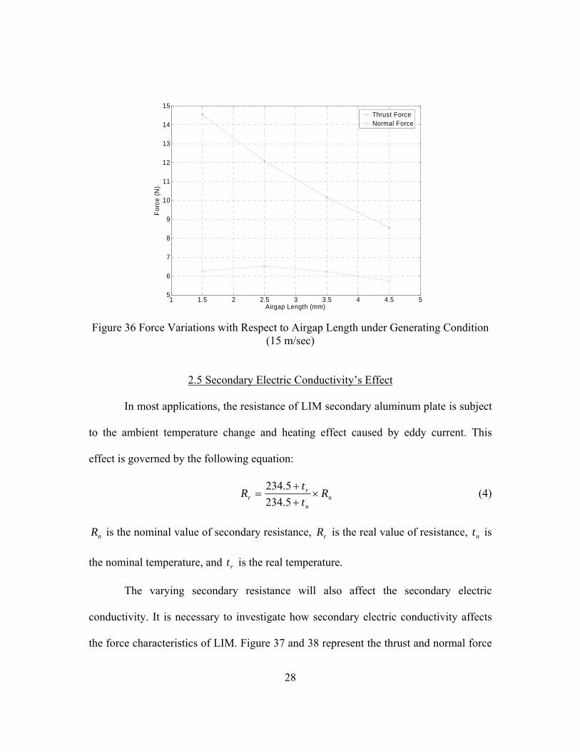
2.4 Airgap Length Effect

The effect of airgap length on the force characteristics of LIM at low linear

speeds has been explored in [1]. Since the force characteristics under high speeds are

more important in propulsion applications, it is necessary to topologies the airgap length

effects for the full speed range.

When linear speed is 1 m/sec (low speed range), and excitation frequency is

36.13 Hz (motoring), the airgap length is varied from 1.5 mm, to 2.5 mm, 3.5 mm, and

4.5 mm in sequence. Figure 31 displays the thrust and normal force variations with

airgap length. The excitation is a set of three phase balanced current sources with

amplitude of 2 A. When excitation frequency changes to 18.16 Hz (electromagnetic

braking), figure 32 represents the force variations with respect to airgap length. From

figure 31 and 32, one can observe that both thrust and normal force monotonically

decrease with airgap length. This phenomenon matches with [1]. Furthermore, linear

speed is increased to 10 m/sec to represent the high speed range. Figure 33 and 34

represent the force variations with respect to airgap length under motoring (116.98 Hz)

and generating (57.26 Hz) conditions respectively. From figure 33, one can notice that

the thrust does not change monotonically any more. The thrust reaches the peak value

when airgap length is 2.5 mm, and then drops. When machine works under generating

condition (figure 34), thrust and normal force monotonically decrease with airgap

length. However, there is a discontinuity in the normal force changing trend. When

linear speed is 15 m/sec, the force characteristics with respect to airgap length under

motoring and generating conditions are shown in figure 35 and 36 respectively. Figure

25

35 shows that the thrust has a maximum value at 3.5 mm airgap length. Compared with

value of figure 33, there is a trend that when linear speed increases the airgap length for

the maximum thrust also increases. In figure 36, the normal force has the maximum

value when airgap length is 2.5 mm. This change is different from that illustrated in

figures 32 and 34.

1 1.5 2 2.5 3 3.5 4 4.5 57

8

9

10

11

12

13

14

15

Airgap Length (mm)

Forc

es (N

)


Figure 31 Force Variations with Respect to Airgap Length under Motoring Condition (1

m/sec)

26

1 1.5 2 2.5 3 3.5 4 4.5 58

9

10

11

12

13

14

15

Airgap Length (mm)

Forc

es (N

)


Figure 32 Force Variations with Respect to Airgap Length under Electromagnetic

Braking Condition (1 m/sec)

1 1.5 2 2.5 3 3.5 4 4.5 55

6

7

8

9

10

11

Airgap Length (mm)

Forc

es (N

)


Figure 33 Force Variations with Respect to Airgap Length under Motoring Condition

(10 m/sec)

27

1 1.5 2 2.5 3 3.5 4 4.5 58

9

10

11

12

13

14

15

16

17

18

Airgap Length (mm)

Forc

es (N

)


Figure 34 Force Variations with Respect to Airgap Length under Generating Condition

(10 m/sec)

1 1.5 2 2.5 3 3.5 4 4.5 54.5

5

5.5

6

6.5

7

7.5

8

Airgap Length (mm)

Forc

es (N

)


Figure 35 Force Variations with Respect to Airgap Length under Motoring Condition

(15 m/sec)

28

1 1.5 2 2.5 3 3.5 4 4.5 55

6

7

8

9

10

11

12

13

14

15

Airgap Length (mm)

Forc

e (N

)


Figure 36 Force Variations with Respect to Airgap Length under Generating Condition

(15 m/sec)

2.5 Secondary Electric Conductivity’s Effect

In most applications, the resistance of LIM secondary aluminum plate is subject

to the ambient temperature change and heating effect caused by eddy current. This

effect is governed by the following equation:

nn

rr R

ttR ×

++

=5.2345.234 (4)

nR is the nominal value of secondary resistance, rR is the real value of resistance, nt is

the nominal temperature, and rt is the real temperature.

The varying secondary resistance will also affect the secondary electric

conductivity. It is necessary to investigate how secondary electric conductivity affects

the force characteristics of LIM. Figure 37 and 38 represent the thrust and normal force

29

variations with respect to secondary electric conductivity at 1 m/sec and 15 m/sec

respectively. One can notice the increment of secondary electric conductivity causes

significant drop of normal force. However, the variation of electric conductivity does

not affect thrust very much. These observations mean that the variation of secondary

electric conductivity can cause significant normal force ripples.

1.5 2 2.5 3 3.5 4 4.5 5 5.5 6x 107

5

10

15

20

25

Electric Conductivity (Siemens/m)

Forc

e (N

)


Figure 37 Force Variation with Secondary Electric Conductivity at Linear Speed 1

m/sec

30

1.5 2 2.5 3 3.5 4 4.5 5 5.5 6x 107

2

4

6

8

10

12

14

16

Electric Conductivity (Siemens/m)

Forc

e (N

)


Figure 38 Force Variation with Secondary Electric Conductivity at Linear Speed 15

m/sec

2.6 Back EMF Characteristics

Figure 39 and 40 are the back EMF amplitude variations with respect to

frequency when linear speed is 1 m/sec and 5 m/sec respectively. For LIM, the thrust

can be related to the electrical input by the following equations:

linear

electricalt V

PF = (5)

)cos()cos()cos( cccbbbaaaelectrical IEIEIEP φφφ ++= (6)

where tF is the thrust force, electricalP is the total electrical power, linearV is the linear

velocity of LIM, nE (n=a, b, or c) is the magnitude of back EMF, nI is the magnitude

of phase current, and nφ is the phase shift between back EMF and phase current. From

figure 39 and 40, it can be observed that when excitation is a set of three phase balanced

31

dc current sources (0 Hz), the amplitude of back EMF is very close to 0. In addition,

when increase excitation frequency to positive or negative infinity, the amplitude of

back EMF increases monotonically. This fact will cause a high stress on power

electronic components when excitation frequency is very high, which may result in

control failure of LIM drive. Based on the data from figure 39 and 40, and equation (5)

and (6), one can plot the phase shift between the back EMF and phase current shown in

figure 41 and 42. Figure 41 has hyperbolic waveforms in first and second quadrants.

Figure 42 has the minimum phase shift at 66.62 Hz, and saturates to 90 degrees in the

positive infinity frequency.

-30 -20 -10 0 10 20 30 400

10

20

30

40

50

60

70

80

Frequency (Hz)

Bac

k E

MF

(V)

Figure 39 Back EMF Amplitude Variation with Frequency at 1 m/sec

32

-100 -50 0 50 100 150 200 250 300 3500

100

200

300

400

500

600

700

800

900

Frequency (Hz)

Bac

k E

MF

(V)

Figure 40 Back EMF Amplitude Variation with Frequency at 5 m/sec

-30 -20 -10 0 10 20 30 4085

90

95

100

105

110

115

120

Frequency (Hz)

Pha

se S

hift

(ele

ctric

al d

egre

e)

Figure 41 Phase Shift between Back EMF and Phase Current at 1 m/sec

33

-100 -50 0 50 100 150 200 250 300 35088

90

92

94

96

98

100

102

Frequency (Hz)

Pha

se S

hift

(ele

ctric

al d

egre

e)

Figure 42 Phase Shift between Back EMF and Phase Current at 5 m/sec

34

CHAPTER 3

FIELD RECONSTRUCTION METHOD OF LINEAR INDUCTION MACHINES

In the last chapter, electromagnetic behavior of LIM has been investigated based

on FEA, and verified by experimental results. FEA is well known and widely used as a

tool for numerical-based analysis of electric machines. However, the computational

effort required to complete a finite element evaluation is significant. Therefore, a so-

called field reconstruction method (FRM) for LIM has been developed. FRM only

requires few number of FEA evaluations to reconstruct the fields in the middle of airgap

for any set of given excitation and positions. Based on the knowledge of fields in the

middle of airgap and Maxwell Stress Tensor (MST) method [29] and [30], one can

predict the forces acting on the primary.

3.1 Background

All force calculations throughout this chapter are based on MST method. Using

MST, the tangential and normal force densities in the middle of airgap can be expressed

as follows:

yxo

x BBfµ1

= (7)

)(2

1 22xy

oy BBf −=

µ (8)

35

where xB and yB are the tangential and normal components of the flux densities in the

middle of airgap of the machine and oµ is the permeability of the air; xf and yf are the

tangential and normal force densities in the airgap. The positive directions of normal

and tangential components are defined in figure 43.

Figure 43 Positive Directions of Normal and Tangential Components

Therefore, the thrust and normal force can be expressed by

dlfzFl

xt ∫= (9)

∫=l

yn dlfzF (10)

where z is the stack length of LIM, nF is the normal force.

36

The following assumptions have been made for the investigation of FRM. The

flux density in the axial direction is zero, which means no end effect is included. The

machine is not saturated, such that the superposition can be applicable. Hysteresis and

eddy currents in the primary and secondary back iron are neglected. The operating

temperature is assumed to be constant. In another word, the heating effect to machine

parameters can be neglected. Furthermore, the primary teeth are assumed to be rigid.

3.2 Basis Function Identification

Based on the assumption of no saturation, the normal and tangential components

of flux density in the middle of airgap can be expressed by the sum of primary and

secondary quantities.

xrxsx BBB += (11)

yrysy BBB += (12)

where xsB and xrB are tangential flux densities of primary and secondary respectively,

and ysB and yrB are normal flux densities of primary and secondary respectively. These

four quantities are also defined as ‘Basis Function’.

3.2.1 Primary Basis Function Derivation

At the first step, a static FEA evaluation is used to derive the primary basis

function of phase a. In the FEA program, primary is fixed in the middle of the

secondary railway to eliminate the railway asymmetry effect on the primary basis

function. In another word, the length of secondary railway is assumed to be infinity. In

addition, phase a current ai is set with 1 A dc current, and phases b and c are open. The

37

normal and tangential flux densities are calculated and stored as basis functions xsaB

and ysaB respectively. In order to store the basis functions, the infinite railway of

secondary is truncated into an effective and finite length. Furthermore, the effective

airgap is discretized into n equally distributed points. Hence, xsaB and ysaB are

represented as two n by 1 vectors in computer. Because of the magnetic asymmetry

effects of primary, in order to calculate the basis functions of phases b and c, the same

procedure for phase a has to be repeated in phase b and c respectively. Figure 44 and 45

illustrate the basis functions of normal and tangential flux densities respectively.

0 50 100 150 200 250 300 350 400-0.01

-0.008

-0.006

-0.004

-0.002

0

0.002

0.004

0.006

0.008

0.01

Position (mm)

Tang

entia

l Flu

x D

ensi

ty (T

)

Primary Basis Function

BxsaBxsbBxsc

Figure 44 Tangential Basis Functions of Three Phases

38

0 50 100 150 200 250 300 350 400-0.015

-0.01

-0.005

0

0.005

0.01

0.015

Position (mm)

Nor

mal

Flu

x D

ensi

ty (T

)


BysaBysbBysc

Figure 45 Normal Basis Functions of Three Phases

Using these basis functions, the flux density contributed by primary with

arbitrary three phase currents can be expressed as follows:

)()()()( lBilBilBilB xsccxsbbxsaaxs ++= (13)

)()()()( lBilBilBilB ysccysbbysaays ++= (14)

where l is the position information on the effective airgap.

3.2.2 Secondary Basis Function Derivation

Unlike xsB and ysB , xrB and yrB are not only determined by the instantaneous

primary current, they are also subject to the change of the primary current. In fact, xrB

and yrB are generated by secondary eddy current, which results from primary current

and primary motion. However, in reality, the electromagnetic forces are only

determined by the slip frequency slipω , which can be expressed as

39

reslipPωωω2

−= (15)

Therefore, slipω is the combined result of electrical and mechanical systems. In

the procedure of FR for LIM, for a given excitation frequency and linear speed, the

electrical angular frequency corresponding to the linear speed is subtracted from the

excitation frequency, and the result is the slip frequency. In order to identify secondary

basis functions, the primary speed is set at 0=v . Using a transient FEA evaluation, an

impulse current is used as phase a current input signal. The impulse input has a value of

1 A at 0t , and 0 elsewhere. A sequence of normal and tangential flux densities for 0tt ≥

is then recorded. Using previously established primary basis functions, the flux

densities generated by secondary eddy current can be represented as follows

xsaximxra BBB −= (16)

ysayimyra BBB −= (17)

where ximB and yimB are the recorded values of flux densities due to the impulse current

input, and xraB and yraB are secondary basis functions of phase a. Using the same

procedure, secondary basis functions of phase b and c can also be identified.

Furthermore, all secondary basis functions are in the format of matrices. The rows of

the matrices represent the n points along the effective airgap; the columns of matrices

describe the impulse response of these points in the time domain. Therefore, the normal

and tangential flux densities due to secondary eddy current can be summarized as

following two equations:

40

),()(),()(),()(),( tlBtitlBtitlBtitlB xrccxrbbxraaxr ∗+∗+∗= (18)

),()(),()(),()(),( tlBtitlBtitlBtitlB yrccyrbbyraayr ∗+∗+∗= (19)

where ‘∗ ’ denotes the operation of convolution.

The two step procedure of basis function identification is shown in figure 46.

Magnetostatic FEA Solution


Derivation

Transient FEA Solution

Secondary Basis Function

Derivation

In = 1 A(n = a, b, c)

Bxsa, Bxsb, Bxsc,Bysa, Bysb, Bysc

+-

Bxra, Bxrb, Bxrc,Byra, Byrb, Byrc

In = 1 A impulse current(n = a, b, c)

ν = 0

X

Step 1

Step 2

Figure 46 Two Step Procedure of Basis Function Identification

41

3.3 Field Reconstruction

Once all basis functions have been identified, the total tangential and normal

flux densities xB and yB in the middle of airgap due to arbitrary primary excitation

current can be obtained as:

),()(),()(),()(

)()()()()()(),(tlBtitlBtitlBti

lBtilBtilBtitlB

xrccxrbbxraa

xsccxsbbxsaax

∗+∗+∗+++=

(20)

),()(),()(),()(

)()()()()()(),(

tlBtitlBtitlBti

lBtilBtilBtitlB

yrccyrbbyraa

ysccysbbysaay

∗+∗+∗+

++= (21)

Since the secondary basis functions are in the discrete time domain, the

operation of convolution in equation (20) and (21) will be conducted in discrete time

domain.

∑∑∑===

−+−+−+

++=k

mmkxrcmc

k

mmkxrbmb

k

mmkxrama

xsckcxsbkbxsakakx

ttlBtittlBtittlBti

lBtilBtilBtitlB

111),()(),()(),()(

)()()()()()(),( (22)

∑∑∑===

−+−+−+

++=k

mmkyrcmc

k

mmkyrbmb

k

mmkyrama

ysckcysbkbysakaky

ttlBtittlBtittlBti

lBtilBtilBtitlB

111),()(),()(),()(

)()()()()()(),( (23)

Finally, using MST the force densities and then electromagnetic forces can be

computed. The procedure is shown in figure 47.

Figure 47 Field Reconstruction Procedure

42

3.4 Verification of Field Reconstruction

To verify the effectiveness of the proposed FR method, the constant speed

operation is simulated. Constant speed operation is useful in evaluation of LIM steady

state performance. In the following session, the comparison between direct FEA, slip

frequency FEA, and FRM will be investigated. The direct FEA is the FEA simulation

including the linear speed. Slip frequency FEA is the transient FEA program that uses

the slip frequency in the excitation instead of real frequency, and does not have linear

motion. FRM is the simulation conducted in Matlab/Simulink that utilizes the slip

frequency excitation method to reconstruct fields of the LIM. Since the experimental

test will be conducted at linear speed of 0.1 m/sec, the linear speed is also set to 0.1

m/sec in the constant speed operation for comparison. The electrical angular frequency

corresponding to 0.1 m/sec is 1 Hz. Therefore when excitation frequency is 51 Hz, the

slip frequency will be 50 Hz. At t = 0 sec, the commanded three phase current are

activated. The flux densities results from both slip frequency FEA and FRM at t = 0.1

sec are shown in figure 48 and 49 respectively. One can notice there is no visual

difference between slip frequency FEA and FRM. Figure 50 and 51 illustrate the normal

flux density variations at the same position from FRM and experiment testbed. The

output of the flux meter to oscilloscope is voltage signal. The amplitude of this voltage

signal is 1.06 V, which is corresponding to about 0.05 T. One can notice the results

from figure 50 and 51 match well.

43

-200 -150 -100 -50 0 50 100 150 200-0.05

-0.04

-0.03

-0.02

-0.01

0

0.01

0.02

0.03

0.04

0.05

Position (mm)

Tang

entia

l Flu

x D

ensi

ty (T

)

Slip Frequency FEAFRM

Figure 48 Tangential Flux Density

-200 -150 -100 -50 0 50 100 150 200-0.06

-0.04

-0.02

0

0.02

0.04

0.06

Position (mm)

Nor

mal

Flu

x D

ensi

ty (N

)


Figure 49 Normal Flux Density

44

0 20 40 60 80 100 120 140 160 180 200-0.06

-0.04

-0.02

0

0.02

0.04

0.06

Time (msec)

Nor

mal

Flu

x D

ensi

ty (T

)

Figure 50 Normal Flux Density in the Middle of Airgap at One Particular Position

Using FRM

Figure 51 Normal Flux Density in the Middle of Airgap at the Same Position with Figure 50 from Experiment (0.05 T/Div)

45

Using MST, the thrust and normal force variations with time are illustrated in

figure 52 and 53 respectively. One can notice in steady state there are small values of dc

error between these three methods. The reason of the dc error between direct FEA and

slip frequency FEA is that the slip frequency FEA has no motion; therefore, there is no

trailing eddy current effect in the slip frequency FEA. The dc error between slip

frequency FEA and FRM is caused by truncating the infinite railway into a finite

effective railway with airgap and using finite discrete time domain convolution. In

addition, one can notice due to the existence of the trailing eddy currents, the thrust

value from direct FEA is less than the value from FRM. In another word, trailing eddy

current can degrade the force performance of LIM.

10 20 30 40 50 60 70 80 90 1000

1

2

3

4

5

6

7

Time (msec)

Thru

st (N

)

Direct FEASlip Frequency FEAFRM

Figure 52 Thrust Variations of Three Methods

46

10 20 30 40 50 60 70 80 90 100-3

-2

-1

0

1

2

3

4

5

6

Time (msec)

Nor

mal

For

ce (N

)


Figure 53 Normal Force Variations of Three Methods

3.5 Saturation Effects

No saturation is one of the fundamental assumptions of FRM. However, it is

necessary to investigate the robustness of FRM to saturation effects. The comparison in

the last session is repeated here. Except the current amplitude, all the other parameters

are the same. In FEA calculation and FRM, the phase current amplitude is changed to

25 A, such that the maximum flux density in primary of LIM is about 1.49 T. This

means the machine has been saturated. Figure 54 and 55 illustrate the flux densities

from both slip frequency FEA and FRM at instant 0.1 sec. One can notice there is some

local visual difference between the results from slip frequency FEA and FRM due to the

existence of saturation effect. However, most part of the waveform matches well.

47

-200 -150 -100 -50 0 50 100 150 200-0.4

-0.3

-0.2

-0.1

0

0.1

0.2

0.3

Position (mm)

Tang

entia

l Flu

x D

ensi

ty (T

)

With Saturation


Figure 54 Tangential Flux Density with Saturation

-200 -150 -100 -50 0 50 100 150 200-0.4

-0.3

-0.2

-0.1

0

0.1

0.2

0.3

0.4

Nor

mal

Flu

x D

ensi

ty (T

)

Position (mm)

With Saturation


Figure 55 Normal Flux Density with Saturation

Figure 56 and 57 represent the resultant force profiles subject to the saturation

effects. One can notice that the steady state dc errors between the three methods

48

increase to 2.5%. FRM can still generate accurate enough results even though the

saturation is existing.

10 20 30 40 50 60 70 80 90 1000

50

100

150

200

250

Time (msec)

Thru

st (N

)With Saturation


Figure 56 Thrust Variations of Three Methods with Saturation

10 20 30 40 50 60 70 80 90 100-100

-50

0

50

100

150

200

Time (msec)

Nor

mal

For

ce (N

)

With Saturation


Figure 57 Normal Force Variations of Three Methods with Saturation

49

CHAPTER 4

INDIRECT FIELD ORIENTED CONTROL OF LINEAR INDUCTION MACHINES

Direct field oriented control directly measures the location of rotor flux axis,

and uses the flux angle to decouple the stator currents into quadrature and direct

components, i.e. qI and dI . qI and dI are also called force and magnetizing current

respectively. The concept of indirect field oriented control is similar to that of direct

field oriented control in which the position of rotor flux in the airgap is estimated. The

control core governed by equation (2) and (3) has been introduced in the chapter 2.

The following assumptions have been made for vector (field oriented) current

control. The system is three phase balanced (or symmetric in space and time). In

addition, the translational magneto-motive force is sinusoidal. Furthermore, the machine

is not saturated.

Traditionally, for rotary induction motor drives vector control can guarantee fast

response because the decoupled qI and dI are dc components and easy to be regulated

by PI controllers. Since LIM inherent similarities with their rotary counterparts, vector

control has been predominantly applied to LIM in the past. However, vector control

does not deliver the maximum force per ampere performance. On the other hand, due to

the existence of trailing eddy current effects and magnetic asymmetry effects,

50

the first two fundamental assumptions on the sinusoidal magneto-motive field and lack

of saturation have been undermined. This in turn influences the expected functionality

of vector control. In the following sessions, details of indirect field oriented control

(IFOC) will be explored.

4.1 Fundamentals of IFOC

Since IFOC does not need the two quadrature flux sensors to measure the rotor

or stator flux, it is more often used. Figure 24 illustrates the block diagram of IFOC,

which is based on equation (2) and (3) from chapter 2. These two equations are recalled

here:

ds

qs

rre i

iPτ

ωω 12

+= (2)

( ) ( )22dsqsrms iiI += (3)

In the diagram, ML is the magnetizing inductance, rrL is the secondary inductance, rr

is the secondary resistance, secondary time constant rτ in equation (2) is defined as

rrr rL / , eθ is the flux angle used to decouple three phase stator current (abc axis) into

dq axis and convert the quantities in dq axis back to abc axis. Under normal condition,

dsi will be regulated at its rated value, commanded qsi is generated through the speed

control loop. The thrust generated by the LIM drive can be expressed by the following

two equations:

qsFt iKF = (24)

lt FDvvMF ++=•

(25)

51

where tF is the thrust, FK is the force constant, M is the total mass of LIM primary

system, D is the viscous friction coefficient, •

v is the acceleration speed, v is the linear

speed.

4.1.1 Identification of Secondary Time Constant

From equation (2) it is observed that implementation of IFOC requires the

LIM’s secondary time constant rτ . The time constant is determined by applying a DC

current of 3A for a short period of time to establish a dc flux across the airgap and

measuring the voltage across one of the excited phases and the third phase. The

measured voltage when the source is removed appears due to the transient that develops

in the secondary. On the removal of the source, the voltage drops and then rises to zero.

The rising profile of the curve gives the time constant of the secondary which is about

40 msec. Figure 58 illustrates the experimental result of secondary time constant

determination.

52

Figure 58 Measurement of Secondary Time Constant (Vertical Axis: Voltage, Horizontal Axis: Time)

4.1.2 Determination of Parameters in dq Axis

In order to harvest the best performance that IFOC can supply, the accurate

information of dsi , qsi , and FK rated values needs to be identified. Equation (2) and (3)

are utilized in this procedure.

At standstill and normal condition, equation (2) and (3) will be modified as

equation (26) and (27) as follows:

rds

rqs

re i

iτ

ω 1= (26)

( ) ( )22 rds

rqs

rrms iiI += (27)

where rqsi , r

dsi , and rrmsI are the rated values of dq axis and phase currents respectively.

53

According to the specification of LIM, the rated phase current is 4 A, and rated

thrust is 7 lbs (31.14 N). In addition, from FRM the maximum standstill thrust occurs

when excitation frequency is 24.43 Hz. This frequency is the rated frequency at

standstill. Based on this information, rqsi and r

dsi can be estimated as following values:

rdsi =0.643 A, r

qsi =3.948 A.

Furthermore, FK can be identified as 8.042 N/A using equation (24).

4.2 Closed Loop Speed Control Using IFOC

In this session, closed loop speed control based on IFOC will be conducted.

This includes simulation study and experiment verification.

4.2.1 Simulation Study of IFOC

In the closed loop speed control, dsi is regulated at its rated value, qsi is

regulated such that it can develop the desired thrust to track the reference speed. Once

dsi and qsi references are generated, they will be transformed back to abc axis to

produce three phase current references. Furthermore, phase current is controlled using

hysteresis control. Figure 59 illustrates the speed control loop of IFOC in

Matlab/Simulink. It mainly comprises of PI controller, saturation block, and LIM plant.

The bandwidth of PI controller should be much less than that of current controller due

to the fact that the mechanical system time constant is much larger. Therefore, qsi

reference can be used in the diagram instead of the real qsi such that equation (24) can

be modified as:

∗= qsFt iKF (28)

54

The block ‘saturation’ is used to prevent the qsi exceeding its normal value. The

total mass M of the LIM primary system is 17 Kg, and the viscous friction coefficient

D is 0.05 N*sec/m.

Figure 59 Block Diagram of Closed Loop Speed Control with IFOC

Based on figure 59, the characteristic equation of the speed control loop is

formulated as follows:

005.017

1**)(1 =+

++

sK

sask

F (29)

k is the proportion coefficient, a is the integration coefficient, and )05.017/(1 +s is

the plant of the LIM. The bandwidth of the PI controller is selected at 20 Hz, and the

damping ratio is 0.9. Based on these parameters, k and a can be computed as 531.3

and 62.8 respectively. However, because of the non-linearity of the saturation block,

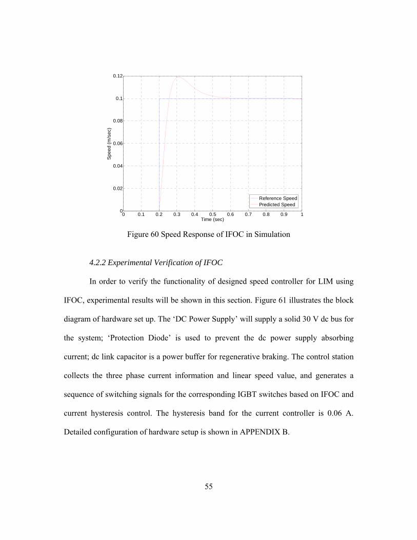
k =80, and a =10 can give best simulation results by trial & error selection. Figure 60

represents the speed response from the simulation. Reference speed steps up to 0.1

m/sec at instant 0.2 sec. The reason that linear speed reference chooses 0.1 m/sec is that

the length of the LIM secondary railway is limited. One can notice that there is an

overshoot about 20% in the speed response, and speed reaches steady state in about 0.4

sec.

55

0 0.1 0.2 0.3 0.4 0.5 0.6 0.7 0.8 0.9 10

0.02

0.04

0.06

0.08

0.1

0.12

Time (sec)

Spe

ed (m

/sec

)

Reference SpeedPredicted Speed

Figure 60 Speed Response of IFOC in Simulation

4.2.2 Experimental Verification of IFOC

In order to verify the functionality of designed speed controller for LIM using

IFOC, experimental results will be shown in this section. Figure 61 illustrates the block

diagram of hardware set up. The ‘DC Power Supply’ will supply a solid 30 V dc bus for

the system; ‘Protection Diode’ is used to prevent the dc power supply absorbing

current; dc link capacitor is a power buffer for regenerative braking. The control station

collects the three phase current information and linear speed value, and generates a

sequence of switching signals for the corresponding IGBT switches based on IFOC and

current hysteresis control. The hysteresis band for the current controller is 0.06 A.

Detailed configuration of hardware setup is shown in APPENDIX B.

56

Figure 61 Block Diagram of Hardware Set Up

Figure 62 illustrates the speed response of a rectangular speed reference at no

load condition. At instant 0 sec, speed reference steps up to 0.1 m/sec, and steps down

to 0 at instant 3.072 sec. One can notice that it takes about 1.5 sec for the speed to reach

its reference value when starting, and 1 sec when braking. This is because when starting

the thrust overcomes the friction force; however, when braking thrust and friction force

will sum together to decelerate the system. In addition, for the initial starting period 0.5

sec, the speed does not change much, that is because the period is utilized for LIM to

overcome the static friction force. Figure 63-65 represent the phase current during

starting, mode transition, and braking under no load condition. One can observe that

when LIM is starting or braking, phase current maintains amplitude of 4 A to generate

the maximum thrust to drive the system. Figure 64 illustrates that in steady state when

linear speed reaches its reference value, the commanded force current *qsi varnishes, as a

57

result, the amplitude of phase current decreases. Thereafter, the operation mode

switches.

0 0.5 1 1.5 2 2.5 3 3.5 4-0.02

0

0.02

0.04

0.06

0.08

0.1

0.12

0.14

Time (sec)

Spe

ed (m

/sec

)No Load

Measured SpeedReference Speed

Figure 62 Speed Response of IFOC from Experiment (No Load)

Figure 63 Phase Starting Current of IFOC (No Load)

58

Figure 64 Transition of Operation Mode of Phase Current in IFOC (No Load)

Figure 65 Phase Braking Current of IFOC (No Load)

59

Figure 66 illustrates the speed response of a rectangular speed reference when a

22 lbs mass is put on top of the primary to increase the friction force and time constant

of the mechanical system. One can notice that compared with no load condition both

slopes of starting and braking are reduced, because the total mass of primary is

increased. From figure 62 and 66, one can observe that in steady state there is a dc error

between the reference speed and measured speed. This is mainly because of the trailing

eddy current effects and magnetic asymmetry effects. In addition, the performance of

the speed controller is restricted by the order of the speed controller.

Figure 67-69 illustrate the phase current during starting, mode transition, and

braking when LIM is loaded by the 22 lbs mass. It can be noticed that the profiles of

phase current when the machine is loaded are very similar to those under no load

condition. In addition, there is certain amount of noise in the current waveform. This is

mainly because the excitation frequency not only depends on linear speeds, but also

relies on the qsi . However, qsi is also a function of linear speed. Therefore, the resultant

excitation frequency will suffer from two sources of noise.

60

0 0.5 1 1.5 2 2.5 3 3.5 4 4.5-0.02

0

0.02

0.04

0.06

0.08

0.1

0.12

0.14

Time (sec)

Spe

ed (m

/sec

)

Heavy Load


Figure 66 Speed Response of IFOC from Experiment (22 lbs Load)

Figure 67 Phase Starting Current of IFOC (22 lbs Load)

61

Figure 68 Transition of Operation Mode of Phase Current in IFOC (22 lbs Load)

Figure 69 Phase Braking Current of IFOC (22 lbs Load)

62

CHAPTER 5

MAXIMUM FORCE PER AMPERE CONTROL OF LINEAR INDUCTION MACHINES

Since the trailing eddy current effects and magnetic asymmetry effects have

prevented IFOC of LIM harvesting its high grade performance, a simple, easy to

implement, and fast response control strategy so called maximum force/ampere control

is proposed and implemented in this chapter.

5.1 Principles of Maximum Force per Ampere Control

Figure 70 and 71 illustrate the average thrust and normal force variations with

respect to primary frequency at different linear speeds. One can notice that at any linear

speed, there is always one pair of excitation frequencies that can produce the maximum

driving force or braking force for the LIM system. These frequencies are characterized

as optimum frequencies. If the gravity force and its by-product, friction force, are also

taken into account, one can summarize the following expression:

aMFgMF nfrictiont ×=+×− )(ξ (30)

where tF is the thrust force, nF is the normal force, frictionξ is the friction coefficient

between LIM and supporting frame, g is the gravity constant, M is total mass of the

LIM system, and a is the acceleration speed of the whole system. Using FRM, one can

always find the pair of optimum frequencies for each linear speed. For example,

63

when linear speed is 5 m/sec, the optimum frequency of motoring is 77.49 Hz, and

optimum frequency of generating is 25.9 Hz.

Based on the knowledge of the optimum frequencies for the discrete linear

speeds and interpolation method, lookup tables between linear speed and optimum

frequency under motoring and generating conditions can be set up. Furthermore, the

optimum frequency is fed into the power converter to produce a set of three phase,

balanced, current sources of optimum frequencies using hysteresis control. As a result,

at any linear speed maximum force/ampere can be guaranteed. Finally, linear speed is

regulated with the usage of hysteresis control. The complete functionality of the

maximum force/ampere control is shown in figure 72. As shown in figure 72, hysteresis

comparator in the block diagram determines whether the machine should work as a

motor or as a generator. This information will be given to the block called ‘Frequency

Selector’. Two lookup tables store the optimum frequencies at discrete linear speeds.

One of the outputs from the lookup tables will be selected based on the operation mode.

The following two expressions can explain the function of ‘Frequency Selector’ in

details:

)(__ motoringff inout = , if HysteresisSpeedSpeed outref >− __ band (31)

)(__ generatingff inout = , if HysteresisSpeedSpeed outref −<− __ band (32)

where outf _ is the output of the frequency selector, )(_ motoringf in and

)(_ generatingf in are the outputs of the two lookup tables, refSpeed _ is the reference

linear speed, and outSpeed _ is the measured linear speed.

64

-100 -50 0 50 100 150 200 250 300 350 400-20

-15

-10

-5

0

5

10

Frequency (Hz)

Thru

st F

orce

(N)

05 m/sec10 m/sec15 m/sec

Figure 70 Average Thrust Variation with Excitation Frequency at Different Linear

Speeds

-100 -50 0 50 100 150 200 250 300 350 400-35

-30

-25

-20

-15

-10

-5

0

5

10

Frequency (Hz)

Nor

mal

For

ce (N

)

05 m/sec10 m/sec15 m/sec

Figure 71 Average Normal Force Variation with Excitation Frequency at Different

Linear Speeds

65

Figure 72 Control Block Diagram for the Maximum Force/Ampere Control

5.2 Simulation Study of Maximum Force per Ampere Control

Figure 73 represents the speed response of a rectangular reference speed. At

instant 0.2 sec, speed reference steps up to 0.1 m/sec, and steps down to zero at instant

0.8 sec. The hysteresis band of the speed regulator is 0.01 m/sec. It is notable that under

accelerating condition, the friction force resists motion; however, under decelerating

condition, the friction force helps the braking. Therefore, figure 73 has larger braking

slope than the one of starting. This is very similar to the phenomenon of figure 62 and

66.

Figure 74 is the simulated optimum excitation frequency profile. It can be

observed that depending on the mode of operation, frequency switches between

motoring (positive frequency) and generating (negative frequency) conditions.

66

0 0.1 0.2 0.3 0.4 0.5 0.6 0.7 0.8 0.9 10

0.02

0.04

0.06

0.08

0.1

0.12

Time (sec)

Spe

ed (m

/sec

)

Reference SpeedPredicted Speed

Figure 73 Speed Response of Maximum Force/Ampere Control

0 0.1 0.2 0.3 0.4 0.5 0.6 0.7 0.8 0.9 1-20

-15

-10

-5

0

5

10

15

20

25

30

Time (sec)

Freq

uenc

y (H

z)

Figure 74 Profile of Optimum Excitation Frequency

Figure 75 illustrates the reference phase current and the predicted phase current

using hysteresis control. Figure 76 is the zoomed version of figure 75.

67

0 0.1 0.2 0.3 0.4 0.5 0.6 0.7 0.8 0.9 1-8

-6

-4

-2

0

2

4

6

8

Time (sec)

Pha

se C

urre

nt (A

)

Reference currentPredicted Current

Figure 75 Simulated Reference Phase Current and Predicted Phase Current

0.72 0.73 0.74 0.75 0.76 0.77 0.78 0.79 0.8-6

-4

-2

0

2

4

6

Time (sec)

Pha

se C

urre

nt (A

)

Reference currentPredicted Current

Figure 76 Zoomed Phase Current Profile

Figure 77 and 78 represent the thrust and normal force ripples with respect to

frequency at linear speed of 5 m/sec. One can notice there is one peak in figure 77. The

68

reason is that when linear speed approaches synchronous speed, the thrust approaches

zero. As a result, even a small value of ripple in the force will cause an extremely large

thrust ripple percentage. However, there are two peaks in figure 78. The reason of the

peak in the negative frequency is that when frequency approaches negative infinity or

positive infinity, normal force changes to repulsion force from attraction force [20].

When normal force is zero, the normal force ripple percentage will be infinity. The

second peak happens when thrust force ripple percentage has a minimum value. When

linear speed is 5 m/sec, the optimum frequency of motoring is 77.49 Hz, and optimum

frequency of generating is 25.9 Hz. Both of these two frequencies will generate

relatively small force ripples at this linear speed. This means that the maximum

force/ampere control has good immunity with respect to force noise.

-100 -50 0 50 100 150 200 250 300 3500

20

40

60

80

100

120

140

160

180

Frequency (Hz)

Thru

st F

orce

Rip

ple

Per

cent

age

(%)

Figure 77 Thrust Ripple Percentage with Respect to Frequency at Linear Speed 5 m/sec

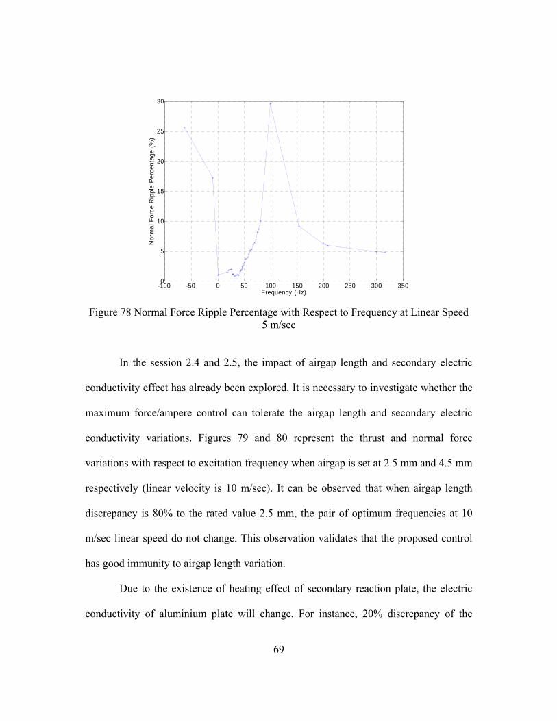
69

-100 -50 0 50 100 150 200 250 300 3500

5

10

15

20

25

30

Frequency (Hz)

Nor

mal

For

ce R

ippl

e P

erce

ntag

e (%

)

Figure 78 Normal Force Ripple Percentage with Respect to Frequency at Linear Speed

5 m/sec

In the session 2.4 and 2.5, the impact of airgap length and secondary electric

conductivity effect has already been explored. It is necessary to investigate whether the

maximum force/ampere control can tolerate the airgap length and secondary electric

conductivity variations. Figures 79 and 80 represent the thrust and normal force

variations with respect to excitation frequency when airgap is set at 2.5 mm and 4.5 mm

respectively (linear velocity is 10 m/sec). It can be observed that when airgap length

discrepancy is 80% to the rated value 2.5 mm, the pair of optimum frequencies at 10

m/sec linear speed do not change. This observation validates that the proposed control

has good immunity to airgap length variation.

Due to the existence of heating effect of secondary reaction plate, the electric

conductivity of aluminium plate will change. For instance, 20% discrepancy of the

70

electric conductivity will result in the real electric conductivity being 31000000

Siemens/m (79% of Aluminum electric conductivity). Figures 81 and 82 illustrate the

force variations with respect to excitation frequency when secondary electric

conductivity is 39000000 Siemens/m (100% of Aluminum electric conductivity) and

31000000 Siemens/m respectively. One can notice that the pair of optimum frequencies

for motoring and generating almost remains the same. Therefore, the proposed

maximum force/ampere control is verified to tolerate the secondary heating effect well.

-100 -50 0 50 100 150 200 250 300 350 400-15

-10

-5

0

5

10

Frequency (Hz)

Thru

st F

orce

(N)

2.5 mm4.5 mm

Figure 79 Thrust Variations with Excitation Frequency for Two Airgap Lengths when

Linear Speed is 10 m/sec

71

-100 -50 0 50 100 150 200 250 300 350 400-20

-15

-10

-5

0

5

10

Frequency (Hz)

Nor

mal

For

ce (N

)

2.5 mm4.5 mm

Figure 80 Normal Force Variations with Excitation Frequency for Two Airgap Lengths

when Linear Speed is 10 m/sec

-100 -50 0 50 100 150 200 250 300 350 400-15

-10

-5

0

5

10

Frequency (Hz)

Thru

st (N

)

79% Al100% Al

Figure 81 Thrust Variations with Excitation Frequency for Two Secondary Electric

Conductivity Values

72

-100 -50 0 50 100 150 200 250 300 350 400-25

-20

-15

-10

-5

0

5

10

Frequency (Hz)

Nor

mal

For

ce (N

)

79% Al100% Al

Figure 82 Normal Force Variations with Excitation Frequency for Two Secondary

Electric Conductivity Values

5.3 Experimental Verification of Maximum Force per Ampere Control

Figure 83 illustrates the speed response under no load condition using maximum

force/ampere control. One can notice that when speed reference steps up to 0.1 m/sec at

0 sec, the speed response is tracking the reference immediately. In addition, the

maximum force/ampere control has excellent speed regulation in steady state.

Furthermore, the braking slope is larger than that of starting.

Figure 84-86 illustrate the transition of phase current from starting to steady

state, from steady state to braking, and during steady state. Figure 86 verifies that

during steady state, depending on the operation mode, excitation frequency switches. In

addition, it has very similar format with the simulated waveform. Furthermore, the

current waveform has less noise than the current waveform from IFOC, because the

73

excitation frequency in maximum force/ampere control only depends on linear speed

once.

0 0.5 1 1.5 2 2.5 3 3.5 4-0.02

0

0.02

0.04

0.06

0.08

0.1

0.12

0.14

Time (sec)

Spe

ed (m

/sec

)No Load


Figure 83 Speed Response of Maximum Force/Ampere Control (No Load)

Figure 84 Transition Phase Current from Starting to Steady State (No Load)

74

Figure 85 Transition Phase Current from Steady State to Braking (No Load)

Figure 86 Zoomed Steady State Phase Current Using Maximum Force/Ampere Control (No Load)

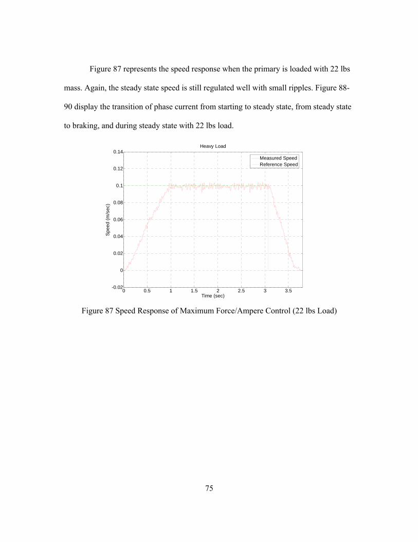
75

Figure 87 represents the speed response when the primary is loaded with 22 lbs

mass. Again, the steady state speed is still regulated well with small ripples. Figure 88-

90 display the transition of phase current from starting to steady state, from steady state

to braking, and during steady state with 22 lbs load.

0 0.5 1 1.5 2 2.5 3 3.5-0.02

0

0.02

0.04

0.06

0.08

0.1

0.12

0.14

Time (sec)

Spe

ed (m

/sec

)

Heavy Load


Figure 87 Speed Response of Maximum Force/Ampere Control (22 lbs Load)

76

Figure 88 Transition Phase Current from Starting to Steady State (22 lbs Load)

Figure 89 Transition Phase Current from Steady State to Braking (22 lbs Load)

77

Figure 90 Zoomed Steady State Phase Current Using Maximum Force/Ampere Control (22 lbs Load)

5.4 Comparison between IFOC and Maximum Force per Ampere Control

As can be seen, the speed response of both methods is plotted together in figure

91 and 92. It can be seen that maximum force/ampere control has faster response and

better regulation on the linear speed.

In addition, the current waveforms from maximum force/ampere control are

much cleaner than those from IFOC. This will result in a smaller value of THD (total

harmonic distortion).

Furthermore, it is necessary to investigate the stability and robustness of the two

methods. Figure 93 and 94 illustrate the linear speed reaction when the 22 lbs mass is

suddenly put on the moving primary in the steady state. In figure 93, at the instant about

0.1 sec, the load is put on the primary, there is a big dip in the speed profile. This is

78

because the design of the PI controller for IFOC is based on the no load LIM plant (17

Kg). The sudden change of load will change the plant immediately. In figure 94, at the

instant about 0.3 sec, the mass is put on the primary, however, the linear speed is not

affected by this disturbance much. The reason is that at any instant the maximum

force/ampere control always generates the maximum force per ampere based on the

current linear speed value.

0 0.5 1 1.5 2 2.5 3 3.5 4-0.02

0

0.02

0.04

0.06

0.08

0.1

0.12

0.14

Time (sec)

Spe

ed (m

/sec

)

No Load

Maximum Force/Ampere Control IFOC Reference

Figure 91 Speed Response of Both Methods (No Load)

79

0 0.5 1 1.5 2 2.5 3 3.5 4 4.5-0.02

0

0.02

0.04

0.06

0.08

0.1

0.12

0.14

Time (sec)

Spe

ed (m

/sec

)

Heavy Load

Maximum Force/Ampere Control IFOC Reference

Figure 92 Speed Response of Both Methods (22 lbs Load)

0.1 0.2 0.3 0.4 0.5 0.6 0.7 0.8 0.9 10

0.02

0.04

0.06

0.08

0.1

0.12

Time (sec)

Spe

ed (m

/sec

)

Disturbance

Figure 93 Speed Profile Subject to a Sudden Change of Load (22 lbs) Using IFOC

80

0.1 0.2 0.3 0.4 0.5 0.6 0.7 0.8 0.9 10

0.02

0.04

0.06

0.08

0.1

0.12

Time (sec)

Spe

ed (m

/sec

)

Disturbance

Figure 94 Speed Profile Subject to a Sudden Change of Load (22 lbs) Using Maximum

Force/Ampere Control

81

CHAPTER 6

CONCLUSIONS AND FUTURTE RESEARCH

Linear induction machine (LIM) offers advantages such as easy maintenance,

simple configuration, and high propulsive performance. Therefore, for the past few

decades linear induction machines have been widely used in transportation, aerospace,

and military. As a result, looking for a high grade control strategy has been a focal area.

Vector control has been a preferred method of control in LIM because LIM possesses

similarities from its rotary counterpart. However, some electromagnetic characteristics

such as trailing eddy current effects and magnetic asymmetry effects have been proven

to undermine the proper functionality of vector control for LIM. In addition, the

investigation on airgap length effect, secondary electric conductivity effect, and back

EMF characteristics has led to development of the in-depth knowledge of LIM

electromagnetic behavior which results in further differences in the way these machines

should be controlled. To address the need for an effective control, a new analysis

method known as field reconstruction method (FRM) has been verified and applied in

LIM. It is more computationally efficient than the traditional tool, i.e. finite element

analysis. In the meantime, FRM also guarantees excellent computational accuracy.

Thereafter, a new control scheme, maximum force/ampere control, is proposed in this

dissertation. Maximum force/ampere control is simple, easy to implement, and fast

82

technique. Both the simulation results and experimental test have validated the

effectiveness of maximum force/ampere control.

On the basis of electromagnetic behavior, field reconstruction method, and

maximum force per ampere control in the linear induction machines, the future research

target should be focused on how to use FRM to detect faults in LIM and how to adopt a

self healing mechanism that can seamlessly recover the drive in the event of a failure in

one of the phases of the machine. Furthermore, advanced magnetic design approaches

can benefit from the fast response of FRM. Finally, it will be desirable to combine the

LIM with the magnetically levitated system (MagLev) to achieve ultra fast frictionless

transportation, and optimize the design of LIM in the context of this application.

83

APPENDIX A

SPECIFICATIONS OF LIM

84

No. Parameter Description

01. Type Linear Induction Machine

02. Power supply 240V, 3 phase AC

03. Winding Configuration wye

04. Poles 4

05. Slots per pole per phase 1

06. Air Gap (mm) 2.5

07. Primary Dimensions in x, y, and z Directions (mm)

250 x 72 x 100

08. Reaction Plate

Dimensions in x, y, and z Directions (mm)

1524 x 3 x 100

09. Back iron Dimensions in

x, y, and z Directions (mm)

1524 x 6 x 100

10.

Material of Primary Lamination

M19

11. Material of Reaction Plate Aluminum: 3.8e7 Siemens/meter

12. Material of Back Iron CR10: Cold rolled 1010 steel

85

APPENDIX B

LIM DRIVE SYSTEM

86

Control Station and DC Power Supply

Interface and Protection Circuit of Linear Position Encoder

Three Phase IGBT Inverter

Control Board and ADC Circuit

87

REFERENCES

[1] I. Boldea, S. A. Nasar, “Linear Motion Electromagnetic System,” John Wiley & Sons Inc., 1995.

[2] S. A. Nasar, I. Boldea, “Linear Motion Electric Machines,” John Wiley & Sons Inc., 1976.

[3] E. R. Laithwaite, “Adapting a Linear Induction Motor for the Acceleration of Large Masses to High Velocities,” Electric Power Applications, IEE Proceedings, Volume 142, Issue 4, July 1995 Page(s): 262-268.

[4] D. J. De Groot, C. J. Heuvelman, “Tubular Linear Induction Motor for Use as a Servo Actuator,” Electric Power Applications, Volume 137, Issue 4, July 1990 Page(s): 273-280.

[5] M. I. Demsky, Yu. P. Vakhrusehin, A. E. Baranovsky, A. A. Volzhev, A. P. Luprianov, D. E. Trifonov, “Linear Induction Accelerators for Industrial Applications,” Particle Accelerator Conference, 1993., Proceedings of the 1993, 17-20 May 1993 Page(s): 682-684 vol.1.

[6] V. Di Dio, M. Montana, “State of Art of Tubular Linear Induction Motor,” Electrotechnical Conference, 1996. MELECON '96., 8th Mediterranean. Volume 1, 13-16 May 1996 Page(s): 285-288 vol.1.

[7] A. Munoz-Garcia, T. A. Lipo, D. W. Novotny, “A New Induction Motor V/F Control Method Capable of High-performance Regulation at Low Speeds,” IEEE Transactions on Industry Applications, Volume 34, Issue 4, July-Aug. 1998 Page(s): 813-821.

[8] S. Srilad, S. Tunyasrirut, T. Suksri, “Implementation of a Scalar Controlled Induction Motor Drives,” SICE-ICASE, 2006. International Joint Conference, Oct. 2006 Page(s): 3605-3610.

[9] I. Ludtke, M. G. Jayne, “Direct Torque Control of Induction Motors,” IEE Colloquium on Vector Control and Direct Torque Control of Induction Motors, 27 Oct. 1995 Page(s): 6/1-6/6.

[10] D. W. Novotny, T. A. Lipo, “Vector Control and Dynamics of AC Drives,” Oxford, U.K.: Clarendon, 1996.

[11] Byung-Il Kwon, Kyung-Il Woo, Sang-Woo Lee, Seung-Chan Park, “Experimental Investigations and Simulations Using FEM for the Direct Field Oriented Control of Linear Induction Motor,” Electric Machines and Drives Conference Record, 1997, IEEE International 18-21 May 1997 Page(s): MC1/10.1-MC1/10.3.

88

[12] E. F. Da Silva, E. B. Dos Santos, P. C. M. Machado, M. A. A. De Oliveria, “Vector Control for Linear Induction Motor,” Industrial Technology, 2003 IEEE International Conference on Volume 1, 10-12 Dec. 2003 Page(s): 518-523 Vol.1.

[13] Rong-Jong Wai, Chia-Chin Chu, “Indirect Field-Oriented Linear Induction Motor Drive with Petri Fuzzy-Neural-Network Control,” Neural Networks, 2005. IJCNN '05. Proceedings. 2005 IEEE International Joint Conference on Volume 1, 31 July-4 Aug. 2005 Page(s): 378-383 vol. 1.

[14] F.-J. Lin, C.-C. Lee, “Adaptive Backstepping Control for Linear Induction Motor Drive to Track Periodic References,” Electric Power Applications, IEE Proceedings- Volume 147, Issue 6, Nov. 2000 Page(s): 449-458.

[15] R.-J. Wai, F.-J. Lin, S.-P. Hsu, “Intelligent Backstepping Control for Linear Induction Motor Drive,” Control Theory and Applications, IEE Proceedings- Volume 148, Issue 3, May 2001 Page(s): 193-202.

[16] A. K. Rathore, S. N. Mahendra, “Simulation of Secondary Flux Oriented Control of Linear Induction Motor Considering Attraction Force & Transverse Edge Effect,” Power Electronics Congress, 2004. CIEP 2004. 9th IEEE International 17-22 Oct. 2004 Page(s): 158-163.

[17] G. Kang, K. Nam, “Field-Oriented Control Scheme for Linear Induction Motor with the End Effect,” Electric Power Applications, IEE Proceedings-Volume 152, Issue 6, 4 Nov. 2005 Page(s): 1565-1572.

[18] Jeong-Hyoun Sung, Kwanghee Nam, “A New Approach to Vector Control for a Linear Induction Motor Considering End Effects,” Industry Applications Conference, 1999. Thirty-Fourth IAS Annual Meeting. Conference Record of the 1999 IEEE Volume 4, 3-7 Oct. 1999 Page(s): 2284-2289 vol.4.

[19] S. Vaez-Zadeh, M. R. Satvati, “Vector Control of Linear Induction Motors with End Effect Compensation,” ICEMS 2005. Proceedings of the Eighth International Conference on Electrical Machines and systems, 2005. Volume 1, 27-29 Sept. 2005 Page(s): 635-638 Vol. 1.

[20] H. Yu, R. Jayabalan, M. Krishnamurthy, B. Fahimi, “Analysis of High Speed Characteristics for Linear Induction Machines,” Vehicle Power and Propulsion Conference, 2006. VPPC’06. IEEE 6-8 Sept. 2006 Page(s): 1-6.

[21] H. Yu, B. Fahimi, “An Investigation on Asymmetry Effects in Linear Induction Machines,” Applied Power Electronics Conference, APEC 2007-Twenty Second Annual IEEE Feb. 2007 Page(s): 390-395.

[22] V. Ostovic, “Computer Aided Analysis of Electric Machine,” Prentice Hall International, UK, 1994.

89

[23] K. Adamisk, J. Mizia, G. E. Dawton, A. R. Eastham, “Finite Element Force Calculation in Linear Induction Machines,” IEEE Transactions on Magnetics, Vol. 1. No. 5. Sep. 1987.

[24] G. E. Dawson, A. R. Eastham, J. F. Gieras, “Design of Linear Induction Drives by Fields Analysis and Finite-element Techniques,” IEEE Transactions, 1986, IA-22, (5), pp. 865-873.

[25] M. A. Al-Maayouf, S. R. Alwash, M. F. Bouniya, “Finite Element Analysis of Linear Induction Motors,” Proc. International Conference on Electric Machine (ICEM), Page(s): 260-266, Munchen, 1986.

[26] W. Zhu, B. Fahimi, and S. Pekarek, “A Field Reconstruction Method for Optimal Excitation of Permanent Magnet Synchronous Machines”, IEEE Transactions on Energy Conversion, vol. 21, no. 2, pp. 305-313, June 2006.

[27] D. Wu, S. D. Pekarek, B. Fahimi, “A Field Reconstruction Technique for Efficient Modeling of the Fields and Forces within Induction Machines,” IECON 2007, Taiwan.

[28] P. C. Krause, O. Wasynczuk, S. D. Sudhoff, “Analysis of Electric Machinery,” IEEE Press, 1995.

[29] I. V. Lindell, B. Jancewicz, “Maxwell Stress Dyadic in Differential-form Formalism,” IEE Proceedings - Science, Measurement and Technology, Volume 147, Issue 1, Jan. 2000 Page(s):19-26.

[30] Z. Ren, A. Rezek, “Force Calculation by Maxwell Stress Tensor in 3D Hybrid Finite Element-boundary Integral Formulation,” IEEE Transactions on Magnetics, Volume 26, Issue 5, Sep 1990 Page(s): 2774-2776.

90

BIOGRAPHICAL INFORMATION

Haidong Yu received his Bachelor of Engineering from Shandong University,

China, in 2003, and M.Sc. in Power Electronics and Motor Drives from the University

of Nottingham, UK, in 2005. He completed Ph.D. in Electrical Engineering in the

University of Texas at Arlington. His research interest includes power electronics,

motor drives, and power quality.

Documents

HIGH GRADE CONTROL OF LINEAR INDUCTION MOTOR DRIVES …