Embed Size (px)
Citation preview

High Data Volume Seismology: Surviving the Avalanche
by
Henry Philip Crotwell
Bachelor of ScienceUniversity of South Carolina, 1992
Master of ArtsUniversity of South Carolina, 1994
————————————————————–
Submitted in Partial Fulfillment of the
Requirements for the Degree of Doctor of Philosophy in the
Department of Geological Sciences
College of Arts and Sciences
University of South Carolina
2007
Major Professor
Committee Member Chairman, Examining Committee
Committee Member Dean of The Graduate School

Acknowledgments
Development of the TauP Toolkit was supported by the University of South Carolina.
Manuscript preparation and software testing were supported by NSF grant EAR-
9304657.
The development of EARS was supported by the EarthScope Program, NSF grant
EAR0346113.
The facilities of the IRIS Data Management System, and specifically the IRIS
Data Management Center, were used for access to waveform and metadata required
in this study. The IRIS DMS is funded through the National Science Foundation and
specifically the GEO Directorate through the Instrumentation and Facilities Program
of the National Science Foundation under Cooperative Agreement EAR-0004370.
ii

ABSTRACT
High Data Volume Seismology: Surviving the Avalanche
Henry Philip Crotwell
Seismic data volumes have increased in the past twenty years with the Incorporated
Research Institutes for Seismology’s Data Management Center currently archiving
upwards of 14 terabytes per year and this trend will continue (Ahern, 2006). Data
volumes are quickly reaching the point at which the individual seismologist can be
overwhelmed with the avalanche of data. We present three studies at the intersection
of seismology and software development that aim to enable more efficient use of data
by practicing seismologists. The first is the TauP Toolkit which calculates the travel
times of seismic waves through custom one dimensional earth models. TauP also
allows almost arbitrary phases to be used and is incorporated into a wide variety of
seismology software. TauP is available at http://www.seis.sc.edu/TauP. The second
is a study of the compression of seismic data, allowing more efficient storage and
transmission. We find that the predictive operator used can have a significant effect on
the compression used, and in many cases second differencing can be noticeably better
than first differencing. The last is the EarthScope Automated Receiver Survey, which
aims to calculate bulk crustal properties for all three component broadband seismic
stations available in the US in a highly automated manner. Because of the high degree
of automation, the project has been extended to calculated crustal thickness and
Vp/Vs for global stations as well. Results are available at http://www.seis.sc.edu/ears.
Dissertation Director: Dr. Thomas J. Owens
iii

Table of Contents
Acknowledgments ii
Abstract iii
List of Figures vii
1 Introduction 1
2 The TauP Toolkit 5
2.1 Introduction . . . . . . . . . . . . . . . . . . . . . . . . . . . . . . . . 5
2.2 Methodology . . . . . . . . . . . . . . . . . . . . . . . . . . . . . . . 6
2.2.1 Slowness Sampling . . . . . . . . . . . . . . . . . . . . . . . . 7
2.2.2 Branch Integration, Phase Summing and Interpolation . . . . 8
2.3 Seismic Phase Name Parsing . . . . . . . . . . . . . . . . . . . . . . . 13
2.4 Velocity Model Descriptions . . . . . . . . . . . . . . . . . . . . . . . 20
2.5 Utilities in the TauP Toolkit . . . . . . . . . . . . . . . . . . . . . . . 21
2.6 Acknowledgments . . . . . . . . . . . . . . . . . . . . . . . . . . . . . 23
3 Compression 24
3.1 Abstract . . . . . . . . . . . . . . . . . . . . . . . . . . . . . . . . . . 24
3.2 Introduction . . . . . . . . . . . . . . . . . . . . . . . . . . . . . . . . 25
3.3 Entropy . . . . . . . . . . . . . . . . . . . . . . . . . . . . . . . . . . 25
3.4 Compression . . . . . . . . . . . . . . . . . . . . . . . . . . . . . . . . 27
iv

3.4.1 Prediction . . . . . . . . . . . . . . . . . . . . . . . . . . . . . 27
3.5 Encoding . . . . . . . . . . . . . . . . . . . . . . . . . . . . . . . . . 31
3.6 Application to Seismic Data . . . . . . . . . . . . . . . . . . . . . . . 32
3.7 Conclusions . . . . . . . . . . . . . . . . . . . . . . . . . . . . . . . . 34
4 EARS 36
4.1 Introduction . . . . . . . . . . . . . . . . . . . . . . . . . . . . . . . . 36
4.1.1 Processing Overview . . . . . . . . . . . . . . . . . . . . . . . 37
4.2 Receiver Functions . . . . . . . . . . . . . . . . . . . . . . . . . . . . 40
4.3 Iterative Deconvolution . . . . . . . . . . . . . . . . . . . . . . . . . . 42
4.4 Determining Crustal Structure . . . . . . . . . . . . . . . . . . . . . . 46
4.5 Phase Weighted Stacking . . . . . . . . . . . . . . . . . . . . . . . . . 49
4.5.1 Analytic Signal . . . . . . . . . . . . . . . . . . . . . . . . . . 49
4.5.2 Phase Weight . . . . . . . . . . . . . . . . . . . . . . . . . . . 50
4.5.3 Application to Hκ Stacking . . . . . . . . . . . . . . . . . . . 51
4.6 Gaussian Width . . . . . . . . . . . . . . . . . . . . . . . . . . . . . . 53
4.7 Error bounds . . . . . . . . . . . . . . . . . . . . . . . . . . . . . . . 56
4.7.1 Curvature error bounds . . . . . . . . . . . . . . . . . . . . . . 57
4.7.2 Bootstrap error bounds . . . . . . . . . . . . . . . . . . . . . . 58
4.8 HKStack Complexity . . . . . . . . . . . . . . . . . . . . . . . . . . . 62
4.9 Comparison and Calibrations . . . . . . . . . . . . . . . . . . . . . . 68
4.9.1 MOMA . . . . . . . . . . . . . . . . . . . . . . . . . . . . . . 68
4.9.2 Zhu and Kanamori . . . . . . . . . . . . . . . . . . . . . . . . 73
4.10 Western US . . . . . . . . . . . . . . . . . . . . . . . . . . . . . . . . 77
Bibliography 83
v

List of Figures
1.1 Growth of the IRIS DMC archive. . . . . . . . . . . . . . . . . . . . . 2
1.2 The 700 stations available in near real time at the IRIS DMC. . . . . 3
2.1 P and S residual for default sampling . . . . . . . . . . . . . . . . . . 10
2.2 P and S residual for coarse sampling . . . . . . . . . . . . . . . . . . 11
2.3 Residual travel time versus ttimes . . . . . . . . . . . . . . . . . . . . 12
2.4 Stylized raypaths for interactions with the 410km discontinuity . . . . 15
2.5 Examples of output from the TauP Toolkit utilities . . . . . . . . . . 22
3.1 Comparison with existing compression ratios . . . . . . . . . . . . . . 33
4.1 EARS Processing System . . . . . . . . . . . . . . . . . . . . . . . . . 39
4.2 Ray paths for P, Ps, PpPs, PsPs and PpSs . . . . . . . . . . . . . . . 41
4.3 Synthetic receiver function . . . . . . . . . . . . . . . . . . . . . . . . 41
4.4 Location of example stations. . . . . . . . . . . . . . . . . . . . . . . 44
4.5 Record section of receiver functions for TA.S08C . . . . . . . . . . . . 45
4.6 Phase weighting versus no phase weighting. . . . . . . . . . . . . . . . 52
4.7 Hκ stack for XA.MM01 for a Gaussian width of 2.5 . . . . . . . . . . 55
4.8 Hκ stack for XA.MM01 for a Gaussian width of 1.0 . . . . . . . . . . 55
4.9 Bootstrap Hκ stacks for TA.S08C . . . . . . . . . . . . . . . . . . . . 60
4.10 Global maximum for each of 100 bootstrap iterations for TA.S08C . . 61
4.11 Hκ stack for BK.CMB . . . . . . . . . . . . . . . . . . . . . . . . . . 63
4.12 Synthetic and Residual Hκ stack for BK.CMB . . . . . . . . . . . . . 64
vi

4.13 Hκ stack for TA.S08C . . . . . . . . . . . . . . . . . . . . . . . . . . 65
4.14 Hκ stack for TA.J06A . . . . . . . . . . . . . . . . . . . . . . . . . . 65
4.15 Complexity versus Crust2.0 Residual . . . . . . . . . . . . . . . . . . 66
4.16 Station Locations within the MOMA array . . . . . . . . . . . . . . . 69
4.17 Crustal thickness comparison with Li et al. (2002) . . . . . . . . . . . 70
4.18 Hκ stacks for MM01, MM11, MM13, MM16, MM17, MM18 . . . . . 72
4.19 Stations in southern California . . . . . . . . . . . . . . . . . . . . . . 74
4.20 Crustal thickness from Zhu and Kanamori (2000) . . . . . . . . . . . 75
4.21 Crustal thickness from EARS in southern California . . . . . . . . . . 76
4.22 Crustal thickness estimates within the western US . . . . . . . . . . . 78
4.23 Cross Section of Juan de Fuca plate . . . . . . . . . . . . . . . . . . . 79
4.24 Thickness estimates for stations in the western US . . . . . . . . . . . 81
vii

Chapter 1
Introduction
The use of computers within seismology has become central within the last few
decades, and the change has enabled huge increases in our ability to learn about
the earth. Many techniques that were simply impossible with paper records have
become commonplace, and led to the increasing reliance of software specific to seis-
mology within the research community. This transition from analog to digital record-
ing has also fueled a tremendous increase in the volume of seismic data available to
researchers over the last two decades. Foremost perhaps is the centralized storage
and dissemination provided by the Incorporated Research Institutes for Seismology’s
Data Management Center, allowing much easier access to existing data. Enhance-
ments to recording systems, following the general increase in computer storage, has
allowed the migration from event-windowed to continuously recorded data, as well as
increases in sampling rates. The IRIS DMC has ingested many new networks over
the years, including regional US networks, foreign national networks and temporary
networks, making these data sets much more readily available. In addition, these
individual networks have increased the number of stations within them. All of these
factors have had a multiplicative effect on data volumes, leading to the change from
a comparative trickle at the beginning of IRIS and the digital recording age to the
veritable flood today shown in Figure 1.1.
1

IRIS DMC Archive GrowthSingle Sort
January 1, 2007
0.0
10.0
20.0
30.0
40.0
50.0
60.0
Jan-9
2
Jul-
92
Jan-9
3
Jul-
93
Jan-9
4
Jul-
94
Jan-9
5
Jul-
95
Jan-9
6
Jul-
96
Jan-9
7
Jul-
97
Jan-9
8
Jul-
98
Jan-9
9
Jul-
99
Jan-0
0
Jul-
00
Jan-0
1
Jul-
01
Jan-0
2
Jul-
02
Jan-0
3
Jul-
03
Jan-0
4
Jul-
04
Jan-0
5
Jul-
05
Jan-0
6
Jul-
06
Jan-0
7
Date
Arc
hiv
e S
ize (
tera
byte
s) EarthScope
PASSCAL
Engineering
US Regional
Other
JSP
FDSN
GSN
Figure 1.1: Growth of the archive of seismic data at the IRIS DMC over the past 25years.
While no one ever wishes for less data, many seismic analysis and processing
techniques of the past can be overwhelmed by this flood if they continue to be used
in the same way. The data volumes have grown by several orders of magnitude,
while the way that seismologists process data has not undergone a similar revolution.
Although the toolkit available to researchers has improved, in many ways the same
scripts are being run, the same manual searches, the same data retrievals and the
same manual processing steps are still employed much as they were a decade ago.
Perhaps because of the limitations of the tools available, most analysis tends to
be done by applying a technique to a given geographical region. While there are
many good reasons to focus on a single locale, in some sense the only natural data
set for seismology is the entire Earth. Except for the constraints of time, there is
2

little reason not to apply a processing system to the entire globe. Of course time is
always in short supply, at least that of the seismologist. However, if a technique can
be automated so that it can continue to process data independent of a person, then
the focus can be expanded to include all available data since computer time is rarely
in short supply. This highly automated processing notion can not only cope with the
increasing volumes of seismic data, but thrives on it, allowing greater use of stacking
and statistics to supplant the “by hand” intensive study of more traditional seismic
processing. Currently there are about 700 stations at the IRIS DMC available in near
real time, shown in Figure 1.2, and only an automated system can hope to deal with
this kind of continual new data. We present three studies at the interface of seismology
and software development: 1D global seismic travel time calculations, compression of
seismic data and automated bulk crustal properties from receiver functions.
Figure 1.2: The 700 stations currently available in near real time at the IRIS DMC.
The first is the TauP Toolkit, an implementation of a global 1D seismic wave
travel time calculator. This brings the ability to calculate travel times within a wide
3

variety of custom earth models as well as for a nearly all seismic phases. The TauP
Toolkit is very flexible and can be embedded within existing applications. Within the
past year there have been almost 500 downloads of the latest version. This chapter
was previously published as Crotwell et al. (1999).
The second is a study of the compression of seismic data, allowing more efficient
storage and transmission of waveforms. The predictive operator used can have a
large impact on the compression ratio, and we find that second differencing can be a
significant improvement over first differencing in many cases.
The last is EARS , the EarthScope Automated Receiver Survey, which demon-
strates a highly automated seismic processing system, capable of handling huge vol-
umes of waveforms. EARS uses receiver functions to calculate bulk crustal properties,
thickness and Vp/Vs , for all broadband three-component seismic stations available
from the Incorporated Research Institutes for Seismology’s Data Management Center
(IRIS DMC). EARS uses the Hκ stacking technique of Zhu and Kanamori (2000)
and to date contains over 180,000 receiver functions for over 1700 stations around the
globe.
4
Chapter 2
The TauP Toolkit
2.1 Introduction
The calculation of travel-times and ray paths of seismic phases for a specified velocity
model of the earth has always been a fundamental need of seismologists. In recent
years, the number of different phases used in analysis has been growing as has the
availability of new earth models, especially models developed from detailed regional
studies. These factors highlight the need for versatile utilities that allow the calcu-
lation of travel-times and raypaths of (ideally) any conceivable seismic phase passing
through (ideally) arbitrary velocity models. The method of Buland and Chapman
(1983) provides significant progress toward this need by allowing for the computa-
tion of times and paths of any rays passing through arbitrary spherically-symmetric
velocity models. The implementation of this method through the ttimes software
program (Kennett and Engdahl , 1991) for a limited number of velocity models and
a standard set of seismic phases has been widely used in the seismological commu-
nity. In this paper, we describe a new implementation of the method of Buland and
Chapman (1983) that easily allows for the use of arbitrary spherically-symmetric ve-
locity models and arbitrary phases. This package, the TauP Toolkit, provides for the
computation of phase travel-times, travel-time curves, raypaths through the earth,
5

and phase piercing-points in a publicly-available, machine-independent package that
should be of use to both practicing seismologists and in teaching environments.
2.2 Methodology
The method of Buland and Chapman (1983) works in the delay (or intercept) time
(τ) - ray parameter (p) domain to avoid complications of multi-valued travel-time
branches associated with working in the time-distance domain directly. Physically,
τ is the zero-distance intercept and p is the slope of the line tangent to the travel-
time curve at a given distance. The advantages of working in this domain are that
τ -branches are monotonic and single valued in all cases, thus do not suffer from the
problems of triplications as their corresponding travel-time branches may in some
circumstances. Furthermore, the ray parameters that define each τ branch are simple
and well-defined functions of the earth model. We will not describe the method in any
detail, but we will discuss the general steps necessary to implement this approach.
We used Maple (Heal et al., 1996), a symbolic mathematics utility, to help convert
the equations in Buland and Chapman (1983) to algorithmic forms for a spherical
coordinate system, avoiding the additional complication of an earth flattening trans-
form. The resulting Maple files are provided with the TauP Toolkit distribution for
those interested in a more detailed study of the methodology.
Generating travel-times using the method of Buland and Chapman (1983) consists
of four major steps. First, sampling the velocity-depth model in slowness. Next,
integrating the slowness to get distance and time increments for individual model
branches. A “branch” of a model is a depth range bounded above and below by local
slowness extrema (first-order discontinuities or reversals in slowness gradients). A sum
of these model branches along a particular path results in the corresponding branch of
the travel time curves. These first two steps are undertaken in the taup create utility
6

and need only be done once for each new velocity model. The third step involves
summing the branches along the path of a specified phase. Finally, an interpolation
between time-distance samples is required to obtain the time of the exact distance of
interest. These final steps are undertaken in various TauP Toolkit utilities, depending
on the information that is desired by the user.
2.2.1 Slowness Sampling
Creating a sufficiently dense sampling in slowness from the velocity models is the
most complicated and crucial step. There are several qualifications for a sufficiently
dense sampling. First, all critical points must be sampled exactly. These include each
side of first-order discontinuities and all reversals in slowness gradient. Less obvious
points that must be sampled exactly occur at the bottom of a low velocity zone.
This sample is the turning point for the first ray to turn below the zone. Note, it is
possible for the velocity to decrease with depth but, due to the curvature of the earth,
there may not be any of the pathological effects. For example, PREM (Dziewonski
and Anderson, 1981) contains a low velocity layer below the moho, but rays turn
throughout it. Hence, a more strictly accurate term might be “high slowness zones”.
A second sampling condition is that slowness samples must be sufficiently closely
spaced in depth. This is normally satisfied by the depth sampling interval of the ve-
locity model itself, but additional samples may need to be inserted. A third condition
is that the sampling interval must be sufficiently small in slowness. We satisfy this
condition by inserting slowness samples whenever the increment in slowness is larger
than a given tolerance, solving for the corresponding depth using the original velocity
model.
Finally, the resulting slowness sampling must not be too coarse in distance, as
measured by the resulting distance sampling for the direct P or S wave from a surface
source. Our approach to satisfying this condition is similar to that of the previous
7

condition. We insert new slowness samples whenever the difference in total distance
between adjacent direct rays from a surface source exceeds the given tolerance. Again,
the depth corresponding to the inserted slowness sample is computed from the original
velocity model. As an additional precaution against undersampling, we also check to
make sure that the curvature is not to great for linear interpolation to be reasonable.
This is accomplished by comparing the time at each sample point with the value
predicted from linear interpolation from the previous to the next point. If this exceeds
a given tolerance then additional samples are inserted before and after the point. The
last two conditions require the most computational effort, but also have the most effect
in creating a sufficiently well-sampled model. The sampling for P and S must meet
these conditions individually and, in order to allow for phase conversions, must be
compatible with each other.
2.2.2 Branch Integration, Phase Summing and Interpolation
For each region, or branch, of the model, we merely sum the distance and time contri-
butions from each slowness layer, between slowness samples, for each ray parameter.
Within each layer we use the Bullen law v(r) = ArB, which has an analytic solution.
The ray parameters used are the subset of slowness samples that correspond to turn-
ing or critically reflected rays from a surface source. Care must be taken to avoid
summing below the turning point for each slowness.
Once these “branches” have been constructed, it is straightforward to create a
real branch of the travel time curves by an appropriate summing. Of course, the
maximum and minimum allowed ray parameter must be determined as well in order
to assure that the ray can actually propagate throughout these regions. For instance,
the branch summing for a P wave turning in the mantle and for PcP are the same.
However, the ray parameter for any P phase must be larger than the slowness at the
bottom of the mantle, while that for PcP must be smaller.
8

Once the sum has been completed to create time, distance and tau as a function
of ray parameter, an interpolation between known points must be done to calculate
arrivals at intermediary distances. Currently, we use a simple linear interpolate which
is sufficient for most purposes. More advanced interpolates do provide advantages in
reducing the number of samples needed to achieve a given accuracy, but they can
have certain instability or oscillatory problems that are difficult to deal with when
the model is not known in advance.
Figure 2.1 and 2.2 summarize the effect of two choices of sampling parameters us-
ing the IASP91 model (Kennett and Engdahl , 1991). In Figure 2.1, we illustrate that
our normal sampling (model file: iasp91) produces a relatively small residual, maxi-
mum of 0.013 seconds for P and 0.016 seconds for S, relative to a highly oversampled
version of the same model generated to produce the most accurate time estimates
without regard to model size or computation time. Thus, model iasp91 is likely the
appropriate choice for travel times that will be used in further computations, for in-
stance earthquake location studies. However, the model size is 337Kb which may be
slow to load on some computer systems and does increase the computation time some-
what. A more coarsely sampled version of IASP91, which we distribute in model file
qdt (quick and dirty times), sacrifices some accuracy for a smaller model file. Figure
2.2 shows qdt residuals with respect to the same highly oversampled model. There
are larger and more noticeable peaks due to linear interpolation between the more
widely spaced samples. While this would not make a good choice for earthquake
location work, an error of 0.25 seconds is entirely satisfactory for classroom work, for
determining windows for extracting phases, and for getting quick estimates of arrival
times. Most important is the fact that the decision of how accurately the model needs
to be sampled is left up to the user. They can easily create new samplings of existing
models tailored to the requirements of the job at hand.
Figure 2.3 compares TauP results using IASP91 to output from ttimes. It would
9

Figure 2.1: First arriving P (top) and S (bottom) residual between a highly oversam-pled IASP91 model and the default sampling. The time residual is sampled everytenth of a degree and is within 0.013 seconds for P and 0.016 seconds for S overthe entire distance range. The slight trend to increasingly negative residuals withdistance is the result of using a less dense linear interpolation of the original cubicIASP91 velocity model. While the difference associated with this trend is small, about0.01 seconds at 180 degrees, adding the ability to read cubic splines directly shouldeliminate it.
10

Figure 2.2: First arriving P (top) and S (bottom) residual between a highly oversam-pled IASP91 model and a coarsely sampled model. This less well sampled versionof IASP91 is referred to as qdt and is shown to illustrate the flexibility of the modelsampling process. It has much larger errors, about + − 0.25 seconds, but is onequarter the size (83Kb) and is therefore more suitable for quick travel time estimates,classroom exercises and web based applications where size and loading speed are morecritical than accuracy. Note the factor of 10 change in scale from the previous figure.
11

Figure 2.3: Residual travel time, this code minus ttimes, of the first arriving P wave(top) and first arriving S wave (bottom). The compressional velocity model wasused throughout the core, so the first arriving S-wave beyond about 80 degrees isSKS and beyond about 130 degrees is SKIKS. The small high frequency oscillations(such as between 50 and 90 degrees) in in the differential times are the result of thelinear interpolant, while the larger offsets are believed to be primarily due to errorintroduced by the earth flattening transform into the ttimes values.
12

be desirable to compare the ttimes output with our own for a model with an easy
analytic solution over a range of distances and phases. Unfortunately, using different
models with the ttimes program has proven difficult. The residual for the direct
comparison with ttimes is shown for the first arriving P wave and S wave. The
calculations are for the IASP91 model for an event at the surface, and are sampled at
0.1 degree increments. The high frequency variations in residuals, such as are observed
between 50 and 90 degrees in the P-wave residuals, are the result of the use of the
linear interpolant in TauP. We believe that the clear trend of increasingly negative
relative residuals with increasing distance is likely related to the use of an earth
flattening transform within the ttimes package, an approximation that can become
problematical toward the center of the earth. The TauP package avoids this potential
complication by working directly in spherical coordinates. To test this assertion, we
compared ttimes and TauP results to travel-times calculated by numerical integration
of vertical rays of PcP, PKIKP, and PKiKP through the IASP91 model. In each case,
our results were closer to the numerical integration results than ttimes with the ttimes
error increasing with increasing depth of penetration. The maximum difference of 0.01
sec for TauP compared to 0.05 sec for ttimes for the vertical PKIKP ray accounts for
the relative P residual shown in Figure 2.3. Thus, we expect that our solutions have
a small, but possibly significant, increase in accuracy relative to ttimes, in spite of
the current simple linear interpolation.
2.3 Seismic Phase Name Parsing
A major feature of the TauP Toolkit is the implementation of a phase name parser
that allows the user to define essentially arbitrary phases through the earth. Thus, the
TauP Toolkit is extremely flexible in this respect since it is not limited to a pre-defined
set of phases. Phase names are not hard-coded into the software, rather the names are
13

interpreted and the appropriate propagation path and resulting times are constructed
at run time. Designing a phase-naming convention that is general enough to support
arbitrary phases and easy to understand is an essential and somewhat challenging
step. The rules that we have developed are described here. Most of phases resulting
from these conventions should be familiar to seismologists, e.g. pP, PP, PcS, PKiKP,
etc. However, the uniqueness required for parsing results in some new names for other
familiar phases.
In traditional “whole-earth” seismology, there are 3 major interfaces: the free
surface, the core-mantle boundary, and the inner-outer core boundary. Phases in-
teracting with the core-mantle boundary and the inner core boundary are easy to
describe because the symbol for the wave type changes at the boundary (i.e. the
symbol P changes to K within the outer core even though the wave type is the same).
Phase multiples for these interfaces and the free surface are also easy to describe be-
cause the symbols describe a unique path. The challenge begins with the description
of interactions with interfaces within the crust and upper mantle. We have introduced
two new symbols to existing nomenclature to provide unique descriptions of potential
paths. Phase names are constructed from a sequence of symbols and numbers (with
no spaces) that either describe the wave type, the interaction a wave makes with an
interface, or the depth to an interface involved in an interaction. Figure 2.4 shows
examples of interactions with the 410km discontinuity using our nomenclature.
14

Figure 2.4: Stylized raypaths for several possible interactions with the 410km dis-continuity to illustrate the use of the TauP phase naming convention. A). Top-sidereflections. In all cases, the upgoing phase could be either upper or lower case sincethe direction is unambiguously defined by the “v” symbol, although lower case is rec-ommended for clarity. B). Transmitted phases. In these cases, there are no alternateforms of the phase names since the symbol case defines the point of conversion fromP to S. C). Underside reflections from a surface source. The “ˆ ” symbol indicatesthat the phases reflect off the bottom of the 410. Final wavetype symbol must beupper case, since lower case wavetype symbols are strictly upgoing. D). Interactionsfor a source depth below the interface. Note that P410s converts on the receiver sidejust as it does for a surface source in B). However, for a deep source, the phase P410Sdoes not exist since a downgoing P-wave cannot generate a downgoing transmittedS-wave at an interface below the discontinuity.
15

1. Symbols that describe wave-type are:
P compressional wave, upgoing or downgoing, in the crust or mantle
p strictly upgoing P wave in the crust or mantle
S shear wave, upgoing or downgoing, in the crust or mantle
s strictly upgoing S wave in the crust or mantle
K compressional wave in the outer core
I compressional wave in the inner core
J shear wave in the inner core
2. Symbols that describe interactions with interfaces are:
m interaction with the moho
g appended to P or S to represent a ray turning in the crust
n appended to P or S to represent a head wave along the moho
c topside reflection off the core mantle boundary
i topside reflection off the inner core outer core boundary
^ underside reflection, used primarily for crustal and mantle interfaces
v topside reflection, used primarily for crustal and mantle interfaces
diff appended to P or S to represent a diffracted wave along the core mantle
boundary
kmps appended to a velocity to represent a horizontal phase velocity (see 10
below)
3. The characters p and s always represent up-going legs. An example is the
source to surface leg of the phase pP from a source at depth. P and S can be
turning waves, but always indicate downgoing waves leaving the source when
they are the first symbol in a phase name. Thus, to get near-source, direct
P-wave arrival times, you need to specify two phases p and P or use the “ttimes
compatibility phases” described below. However, P may represent a upgoing leg
in certain cases. For instance, PcP is allowed since the direction of the phase
16

is unambiguously determined by the symbol c, but would be named Pcp by a
purist using our nomenclature.
4. Numbers, except velocities for kmps phases (see 10 below), represent depths at
which interactions take place. For example, P410s represents a P-to-S conver-
sion at a discontinuity at 410km depth. Since the S-leg is given by a lower-case
symbol and no reflection indicator is included, this represents a P-wave con-
verting to an S-wave when it hits the interface from below. The numbers given
need not be the actual depth, the closest depth corresponding to a discontinuity
in the model will be used. For example, if the time for P410s is requested in a
model where the discontinuity was really located at 406.7 kilometers depth, the
time returned would actually be for P406.7s. The code “taup time” would note
that this had been done. Obviously, care should be taken to ensure that there
are no other discontinuities closer than the one of interest, but this approach
allows generic interface names like “410” and “660” to be used without knowing
the exact depth in a given model.
5. If a number appears between two phase legs, e.g. S410P, it represents a trans-
mitted phase conversion, not a reflection. Thus, S410P would be a transmitted
conversion from S to P at 410km depth. Whether the conversion occurs on the
down-going side or up-going side is determined by the upper or lower case of the
following leg. For instance, the phase S410P propagates down as an S, converts
at the 410 to a P, continues down, turns as a P-wave, and propagates back
across the 410 and to the surface. S410p on the other hand, propagates down
as a S through the 410, turns as an S, hits the 410 from the bottom, converts
to a p and then goes up to the surface. In these cases, the case of the phase
symbol (P vs. p) is critical because the direction of propagation (upgoing or
downgoing) is not unambiguously defined elsewhere in the phase name. The
17

importance is clear when you consider a source depth below 410 compared to
above 410. For a source depth greater than 410 km, S410P technically cannot
exist while S410p maintains the same path (a receiver side conversion) as it
does for a source depth above the 410.
The first letter can be lower case to indicate a conversion from an up-going ray,
e.g. p410S is a depth phase from a source at greater than 410 kilometers depth
that phase converts at the 410 discontinuity. It is strictly upgoing over its entire
path, and hence could also be labeled p410s. p410S is often used to mean a
reflection in the literature, but there are too many possible interactions for the
phase parser to allow this. If the underside reflection is desired, use the p^ 410S
notation from rule 7.
6. Due to the two previous rules, P410P and S410S are over specified, but still
legal. They are almost equivalent to P and S, respectively, but restrict the
path to phases transmitted through (turning below) the 410. This notation
is useful to limit arrivals to just those that turn deeper than a discontinuity
(thus avoiding travel time curve triplications), even though they have no real
interaction with it.
7. The characters ^ and v are new symbols introduced here to represent bottom-
side and top-side reflections, respectively. They are followed by a number to
represent the approximate depth of the reflection or a letter for standard dis-
continuities, m, c or i. Reflections from discontinuities besides the core-mantle
boundary, c; or inner-core outer-core boundary, i, must use the ^ and v no-
tation. For instance, in the TauP convention, p^ 410S is used to describe a
near-source underside reflection.
Underside reflections, except at the surface (PP, sS, etc.), core-mantle bound-
ary (PKKP, SKKKS, etc.), or outer-core-inner-core boundary (PKIIKP, SKJJKS,
18

SKIIKS, etc.), must be specified with the ^ notation. For example, P^ 410P and
P^ mP would both be underside reflections from the 410km discontinuity and the
Moho, respectively.
The phase PmP, the traditional name for a top-side reflection from the Moho
discontinuity, must change names under our new convention. The new name is
PvmP or Pvmp while PmP just describes a P-wave that turns beneath the Moho.
The reason the Moho must be handled differently from the core-mantle bound-
ary is that traditional nomenclature did not introduce a phase symbol change
at the Moho. Thus, while PcP makes sense since a P-wave in the core would be
labeled K, PmP could have several meanings. The m symbol just allows the user
to describe phases interaction with the Moho without knowing its exact depth.
In all other respects, the ^ -v nomenclature is maintained.
8. Currently, ^ and v for non-standard discontinuities are allowed only in the
crust and mantle. Thus there are no reflections off non-standard discontinuities
within the core, (reflections such as PKKP, PKiKP and PKIIKP are still fine).
There is no reason in principle to restrict reflections off discontinuities in the
core, but until there is interest expressed, these phases will not be added. Also,
a naming convention would have to be created since “p is to P” is not the same
as “i is to I”.
9. Currently there is no support for PKPab, PKPbc, or PKPdf phase names. They
lead to increased algorithmic complexity that at this point seems unwarranted.
Currently, in regions where triplications develop, the triplicated phase will have
multiple arrivals at a given distance. So, PKPab and PKPbc are both labeled just
PKP while PKPdf is called PKIKP.
10. The symbol kmps is used to get the travel time for a specific horizontal phase
velocity. For example, 2kmps represents a horizontal phase velocity of 2 kilome-
19

ters per second. While the calculations for these are trivial, it is convenient to
have them available to estimate surface wave travel times or to define windows
of interest for given paths.
11. As a convenience, a ttimes phase name compatibility mode is available. So ttp
gives you the phase list corresponding to P in ttimes. Similarly there are tts,
ttp+, tts+, ttbasic and ttall.
2.4 Velocity Model Descriptions
This version of the TauP package supports two types of velocity model files. Both are
piecewise linear between given depth points. Support of cubic spline velocity models
would be useful and may be implemented in a future release.
The first format is the “tvel” format used by the most recent ttimes code (Kennett
et al., 1995). This format has two comment lines, followed by lines composed of depth,
Vp, Vs, and density, all separated by whitespace. TauP ignores the first two lines
and reads the remaining ones.
The second format is based on the format used by Xgbm (Davis and Henson,
1993). We refer to it as a “named discontinuity” format. Its biggest advantage is
that it can specify the location of major boundaries in the earth. It is our preferred
format. The format also provides density and attenuation fields, which will more
easily accommodate the calculation of synthetic seismograms in the future.
The distribution comes with several standard velocity models. Users can create
their own models by following examples in the User’s Guide included in the distri-
bution package. Standard models are: IASP91 (Kennett and Engdahl , 1991), PREM
(Dziewonski and Anderson, 1981), AK135 (Kennett et al., 1995), Jeffries-Bullen (Jef-
freys and Bullen, 1940), 1066a and 1066b (Gilbert and Dziewonski , 1975), PWDK
(Weber and Davis , 1990), SP6 (Morelli and Dziewonski , 1993), Herrin (Herrin, 1968).
20

2.5 Utilities in the TauP Toolkit
There are 8 separate utilities in the TauP Toolkit. Each is described in detail in the
User’s Guide, so descriptions here are brief. Figure 2.5 summarizes the outputs of
several of the codes.
1. taup create. This utility takes a velocity model in one of the two supported
formats and does the sampling and branch integration processes to produce a
TauP model file for use by all other utilities.
2. taup time. This is the TauP replacement for the ttimes program. At a mini-
mum, given phase, distance and depth information, it returns travel times and
ray parameters. Options allow for station and event locations to be provided in
lieu of distance as well as for more specialized outputs.
3. taup curve. Produces entire travel time curves for given phases. Options
include the ability to output these curves in a format suitable for plotting with
GMT (Wessel and Smith, 1991).
4. taup path. Calculates ray paths for given phases. Options include the ability
to output these paths in a format suitable for plotting with GMT (Wessel and
Smith, 1991).
5. taup pierce. Calculates piercing points at model discontinuities and at speci-
fied depths for given phases. Options include the ability to output these points
in a format suitable for plotting with GMT (Wessel and Smith, 1991).
6. taup setsac. Utility to fill SAC (Tull , 1989) file headers with theoretical arrival
times.
7. taup table. Utility to generate travel time tables needed for earthquake loca-
tion programs. Currently, only an ASCII table format is supported along with
21

0˚
30˚
60˚
90˚
120˚15
0˚
180˚
210˚
240˚
270˚
300˚33
0˚
s
sSources
180˚
180˚
240˚
240˚
300˚
300˚
0˚
0˚
60˚
60˚
120˚
120˚
180˚
180˚
-90˚ -90˚
-60˚ -60˚
-30˚ -30˚
0˚ 0˚
30˚ 30˚
60˚ 60˚
90˚ 90˚
A
C
Red
uced
Tim
e, V
r=0.
125
deg
/sec
D is tance (deg )
s^410PS^670PPms
900
1000
1100
1200
1300
1400
1500
900
1000
1100
1200
1300
1400
1500
100 120 140 160 180
100 120 140 160 180
SS
SKKS
PPP
B
Figure 2.5: Examples of output from the TauP Toolkit utilities. Some modificationsin a touch-up program were done to prepare the figures for publication. A). Outputof taup path for the phase sˆ 410PSˆ 670PPms at a distance of 155 degrees from anevent at 630 km depth. sˆ 410PSˆ 670PPms arrives from both directions, one raytraveling 155 degrees, the other 205 degrees. The model PREM is used. Source isgiven by the *, station by the triangle. B) Output of taup curve for the same phase asin A). A reducing velocity of 0.125 deg/s was used for this plot. Travel-time curves forPPP, SS, and SKKS are shown for reference. C) Output of taup pierce for the samephase as A) was added to an existing GMT script to produce this output. Pointsof interaction with the 400km discontinuity are shown for a hypothetical event nearEast Pacific rise arriving at a hypothetical station in central India. The path for theray that travels 155 degrees to the station is shown in a solid line, interaction pointswith the 400km discontinuity are solid diamonds. The 205 degree raypath is shownas a dashed line with solid circles indicating interaction points at 400km depth.
22

a generic output. Other formats could be supported if interest warrants.
8. taup peek. Debugging code to examine contents of a taup velocity model file.
The TauP Toolkit is written entirely in the Java programming language. This
should facilitate use of the utilities on any major computer platform. It has been
tested on Solaris UNIX, MacOS, and Windows95. The distribution includes simple
scripts to facilitate use of the above utilities in a UNIX environment. It also pro-
vides mechanisms for accessing the utilities via C programs and TCL (via the “jacl”
implementation) scripts. At present, only raw Java command line interfaces exist,
limiting the usefulness in MacOS and Windows environments. A WWW based applet
interface was tested by our undergraduate geophysics course in the Spring of 1998,
however a more refined GUI is planned for development soon which should make the
package much more useful in non-UNIX environments. The package can be obtained
from http://www.seis.sc.edu/taup.
2.6 Acknowledgments
Development of this software was supported by the University of South Carolina.
Manuscript preparation and software testing were supported by NSF grant EAR-
9304657.
23

Chapter 3
Compression
3.1 Abstract
With the larger volumes and growing use of near real time data transmission, im-
proved compression of seismic data is increasingly important. The algorithms in
use within the seismological community do not take advantage of current techniques
within the larger computer science community nor do they take advantage of all of
the properties of seismic time series. We introduce a new scheme for the loss-less
compression of seismic data drawing upon general purpose compression techniques as
well as analysis of the properties of seismic time series. Compression of time series
can be effectively broken into two independent processes operating in series. The
first is a prediction process that transforms the original time series into an equivalent
time series of prediction residual whose values are more closely clustered around zero
than the original. The best balance of quality and speed seems to be first, second
and third differences, with the choice depending on the actual data to be compressed.
The second process is an efficient encoding of the residuals from the prediction pro-
cess. Huffman encoding is one of two widely used methods in the computer science
community, and is simpler to implement and understand than arithmetic encoding.
Current compression algorithms for seismic data concentrate on the encoding process,
24
with little flexibility given to prediction. We propose that a wider choice of prediction
operators can have a major impact on compression ratios, and existing compression
algorithms could benefit with minimal change by allowing second and third differ-
encing. Huffman encoding provides an attractive and efficient encoding scheme, and
has the additional advantage of being widely accepted and used within the broader
computational community.
3.2 Introduction
The volume of seismic data collected and archived has grown tremendously since
the advent of digital recording and rate of growth is increasing. The IRIS Data
Management Center currently archives in excess of 10 terabytes of data per year
and is likely to only increase. At these levels of data flow, even moderate increases
in effectiveness of data compression can have a significant on the required archive
storage space.
Current algorithms widely used within seismology include the Steim1, Steim2 and
US National Network compression. Each of these specifies a first differencing scheme
followed by an encoding with keys and values where the key specifies how many bits
the value uses. These are generally effective at reducing the storage size of data.
3.3 Entropy
A useful concept from information theory is that of entropy. Entropy is a measure-
ment of how much information a data stream carries. One way to define this is to
separate the signal into two parts, a predictable part and an unpredictable part. The
predictable part does not need to be transmitted in order for the receiver to recon-
struct the original signal. The unpredictable part, on the other hand, represents the
disorder in the data stream and must be transmitted. Entropy is the measure of
25

disorder in a thermodynamic system and so the same term is used to measure this
unpredictable part, which is the information content of a data stream. It may seem
contradictory at first to equate disorder with information content, however, a data
stream that is perfectly predictable carries no information and has no disorder. In
a completely unpredictable data stream, by contrast, every single bit is needed to
reconstruct the input values.
Entropy is expressed as the average number of bits needed, per sample, to recover
the original signal. This establishes a lower bound on the size of any compressed
version of the data and thus gives a mile-post to compare effectiveness of compression
algorithms. In the case of a signal where each sample is independent of the previous
sample, the entropy can be defined as
E = −∑i∈N
pi log2(pi) (3.1)
where the sum is over all symbols in the alphabet. The alphabet for a particular
stream of seismic data, for instance, might be all numbers expressible as 32 bit in-
tegers. It is more complicated in the case where the next sample has a complicated
dependence on the previous samples. Knowing the entropy, the redundancy within
the data stream can be defined by
R = log2(N )− E (3.2)
where N is the size of the alphabet.
Although seismic data almost certainly does have dependence on previous samples
even after differencing, it is generally useful to make the assumption of independence.
If there was a known relationship between the current value and previous values,
we could simply apply the corresponding correction to the predictive operator, and
arrive at the assumption of independence. In addition, even if there is dependence,
26

theoretical best compression for an encoder that cannot make use of the dependence
is still bounded by this definition of entropy.
3.4 Compression
The compression of many types of time series in general, and seismic data in par-
ticular, can be modeled as the combination of two processes, a predictive operator
and a mechanism for efficiently encoding the residual of the prediction. The resid-
ual is hopefully composed of very frequently occurring small values and less frequent
large values. It is important to realize that these two operations are independent, the
choice of encoding need not determine the choice of prediction.
3.4.1 Prediction
The predictor is a function that, given information on some number of previous
samples, returns a prediction of the next sample. This predictor need not return
the actual value of the next sample, clearly this is not possible. Rather, it merely
needs to have errors, or residuals, that are on average smaller in absolute value than
the sample. The decompresser, knowing the predictive operator and the previous
samples, can simply perform the inverse operation to recover the true value of the
current sample.
The ability of the predictor to concentrate the residual values around zero is very
important to achieving a good compression. Existing seismic compression algorithms
tend to use a single fixed order of differencing as a simple predictor, for example
the first differencing in the widely used Steim1 and Steim2 algorithms. Options
for predictive operators include first difference, P (n) = f(n − 1), as well as the no-
differencing or null operator, P (n) = 0, second difference, P (n) = 2f(n−1)−f(n−2)
and third difference, P (n) = 3f(n − 1) − 3f(n − 2) + f(n − 3). There are of course
27

others of higher orders. We have found that prediction should be allowed to vary based
on properties of channel for best results. In fact in many cases, second differences
can be as big an improvement over first differencing as first differencing is over no
differencing. Third differences can be better than second for some channels.
The residual of a predictor operating on a time series is also a time series. And
in fact, it can be of the same length as the input if a sufficient number of zeros
are prepended to account for the order of differencing. This eliminates any need for
storing integration constants in a special way at the beginning of the compressed
stream. For example, if second differencing is used then prepending two zeros to
the stream before differencing results in an output stream of the original length. If
the original series, prepended with two zeros, is 0, 0, t1, t2, t3,..., then the second
differenced stream is t1, t2 − 2t1, t3 − 2t2 + t1, ... Notice that nothing special is
done for the first two samples. In addition, if t1 and t2 are of approximately the same
magnitude, no additional space it required as t2−2t1 ≈ −t1. If this technique is used,
any time series encoding, such as Steim1, can be used with any order of differencing,
such as second differences, to achieve the best compression for the given input series.
One possible flaw can occur if t2 − 2t1 is greater than the size of the storage, for
example if t2 − 2t1 was greater than 231. This is not a problem with current data as
they are limited in size due to the commonly used 24 bit digitization.
Deciding which level of differencing to use can be done by computing some basic
statistics for a small, typical time series for a channel, and then assuming that the
background noise levels and spectral characteristics will not change significantly over
time. This is likely reasonable in most cases, but periodic checking is easy and may
be wise. In general, the encodings used depend on most of the values being clustered
around 0. In other words we can use the minimization of the mean and standard
deviation of the residual series as a proxy for compressibility. As a practical matter,
we can ignore minimizing the mean, because if the best predictor, P , resulted in a
28

series with a mean of µ = µ0 6= 0, then we could form a new predictor P ′ = P − µ0
which has mean zero. Our experience has been that first, second and third differencing
result in a series with very near zero mean. Thus, the computation of the best order
of differencing to use reduces to minimizing the standard deviation, which results in
a few values around zero with high frequency of occurrence and the rest of the values
with a low frequency of occurrence.
There are instances where a drifting sensor may cause a bias in the mean. For
instance, suppose a sensor drifts from a mean near zero to a mean near 100,000 over a
period of 1000 samples. The average value of the first differences will be 100 since this
is the average increase per sample. However the effect is limited to either a series of
small differences over a long period of time, or a series of large difference over a short
period of time simply because a large rate of increase will quickly peg the sensor. In
either case, it is unlikely to has a significant effect on the compression over the long
term.
It might seem that if first differencing reduces the standard deviation, then second
should be better, and third even better. In fact, a minimum is usually reached very
quickly, and the results get progressively worse with higher orders. For example, first
differencing of the simple time series shown in the first row of Table 3.1 results in an
improvement, with the mean smaller by more than a factor of 10 and the standard
deviation dropping from 3.56 to 2.22. Second differencing results in another improve-
ment, with the mean smaller and standard deviation of 1.81. However, subsequent
differencing actually results in an increased standard deviation, and hence third dif-
ferencing is actually a worse predictor than first or second differencing. Conceptually,
one can think of differencing as reducing the amplitude of lower frequency signals in
the time series while exaggerating the frequencies near the Nyquist. Consider a sine
wave sampled exactly at the peaks and troughs, giving a series 1,−1, 1,−1, . . . Dif-
ferencing in this case would double the amplitude, yielding −2, 2,−2, 2, . . . Clearly
29

Diff Time Series µ σ0 5 8 10 13 14 13 12 10 8 7 5 4 6 8 10 13 16 9.53 3.561 5 3 2 3 1 -1 -1 -2 -2 -1 -2 -1 2 2 2 3 3 0.94 2.222 5 -2 -1 1 -2 -2 0 -1 0 1 -1 1 3 0 0 1 0 0.18 1.813 5 -7 1 2 -3 0 2 -1 1 1 -2 2 2 -3 0 1 -1 0.00 2.72
Table 3.1: Effect of three differencing schemes (first, second and third differences)on a sample time series. First order differencing makes a large improvement in meanalthough with an increase in standard deviation. Second and third differencing are notan improvement in this case, both leading to increased mean and standard deviationover first differences.
the standard deviation is not reduced in this case.
When the time series is dominated by relatively longer period energy, differencing
results in a net improvement. Once the short periods come to dominate, further
differencing increases the number of large values and hence the standard deviation.
While differencing is the natural first guess at predictive operators, they generalize
to a whole class of predictors known as ARIMA (Box and Jenkins , 1976). These
were originally created for forecasting business phenomena, but are applicable to a
wide range of time series. The generalization involves first applying differencing to
the best order possible, and then creating an additional predictor that uses a linear
combination of both the previous n samples, as well as the last n predictions or
equivalently the last n residuals. The name ARIMA comes from auto-regressive for
the use of the last samples, integral for the differencing, and moving average for the
use of the residuals.
While this generalization seems to open a wide array of possible predictions, we
have not found it to give significant improvements over simply using the best order of
differencing. With the increase complication and the difficulties of using floating point
operations across different computer architectures, we believe that limiting predictors
to differencing is the most practical choice.
30

3.5 Encoding
Once the predictive operator has reduced the magnitudes of the samples, it remains
to efficiently encode them, taking advantage of the fact that the residual has smaller
variance. There are various means of doing this, with the current seismological algo-
rithms using flags to identify the number of bits used for the next sample or samples.
The encoding of the residual time series values is not something unique to seismology,
and hence looking to the domain of computer science is wise. There are two main
encoding schemes in wide use for compression in general, Huffman and arithmetic
encoding, that both achieve near optimal encoding.
Arithmetic encoding (MacKay , 2003) is the more complicated, although with
the advantage of achieving optimal encoding, ie encoding is at the level of entropy.
Huffman is simpler and while it only achieves optimality in certain cases, the difference
for seismic data is not likely significant. We have chosen to use Huffman codes.
Many good references can be found on Huffman encoding, (Huffman, 1952; MacKay ,
2003), and so we only give a brief overview. The basis of Huffman codes is to gener-
ate a binary code for each “letter” of a given alphabet such that the most frequently
appearing letters receive the shortest codes. It seeks to minimize Σfili where fi is
the frequency of the ith letter and li is the length of the code. It is apparent that the
code will achieve optimal compression, ie entropy, if li = log2(fi). In other words, if
all of the frequencies are integral powers of 2. As this is rarely the case, the outcome
will be slightly worse than optimal.
One other important criteria for a successful coding scheme that uses variable
length codes is the prefix property. It requires that no code can be a prefix of another
code. This is readily seen to be necessary for decompression as it would be impossible
to tell whether the code stopped at the end of the prefix, or continued on. What is
not so obvious is that the prefix property is also sufficient for decompression.
To use Huffman encoding, we must define the alphabet. The natural alphabet
31

for seismic data is all integers i with −223 <= i <= 223. This is also not practical.
Instead, we use Huffman codes for a subrange of this natural alphabet that contains
the bulk of the frequently occurring values and then use an escape code to deal with
the occasional value outside of that range. We have found ranges of ±210or ± 212
have reasonable trade offs between size and compressibility. Even for noisy stations,
an insignificant number of samples lie outside of this range once an appropriate order
of differencing has been applied.
The other requirement for building Huffman codes is the frequency of occurrence of
each value within the alphabet. We can assume seismic background noise is very close
to a normal distribution, and hence we need only calculate the standard deviation in
order to characterize the frequency distribution. This single measurement allows the
Huffman codes to be tuned to best compress the time series.
3.6 Application to Seismic Data
We have applied our compression algorithm to seismic data from the IRIS DMC.
Figure 3.1 shows a histogram of the ratio of the original compression, either Steim1
or Steim2 (Ahern and Dost , 2006), to this algorithm. The majority of the data com-
presses better with this algorithm than the existing ones. The total size of the original
compressed data was 149 Mb. Using our algorithm, the sizes are 137 Mb, 128 Mb and
139 Mb using first, second and third differencing respectively. If instead of picking a
single difference order we choose the best order of differencing for each seismogram,
the size is 123 Mb, an improvement of over 17%. With this dataset, second differ-
encing is clearly the best single choice, and picking the order of differencing on a per
seismogram basis can do even better.
32

Figure 3.1: Histogram of the ratio existing compression algorithms at the IRIS DMC,mostly Steim1 and Steim2, to this algorithm. The data was all BHZ seismogramsat IU stations for all magnitude 6 or larger earthquakes in January of 2006. Therequest was for 1 hour of data starting 2 minutes before the P arrival, althoughdata availability affects this. The majority of the data compressed better with ouralgorithm.
33

3.7 Conclusions
We have found that the choice of predictive operator or equivalently order of dif-
ferencing is critical to achieving near optimal compression of seismic data. Simply
using first differences in a “one size fits all” approach sacrifices the additional com-
pression possible for channels where second, and even third, differences provide very
real improvements.
Huffman codes, while more complex at first glance than the traditional seismic
encoding schemes, are effective, and achieve near optimal compression. They are a
standard within the broader realm of data compression in general, being used in the
popular general purpose compression tools. They have the added benefit of being
capable of being tuned to best encoded the given data stream, taking utmost advan-
tage of streams that have very small variances, while still being able to able to handle
difficult to compress high variance data streams.
Disadvantages of the Huffman codes include the fact that they are not byte aligned,
which trades off speed for increased compression. The increased compression ratios
seem worth the small speed penalty. They are conceptually more difficult to under-
stand because of the varying length codes, but the algorithm need only be understood
in detail by the software engineers that will implement the compression and decom-
pression routines.
One additional difficulty is the need for floating point operations in creating the
Huffman codes. While using the actual standard deviation of the stream creates the
best codes, the penalty for using a close standard value may not be too great. For
example codes could be pre-generated for standard deviations of 4, 8, 16, 32,. . . , 4096,
which cover a wide range from very quite to very noisy channels, while still keeping
the codes relatively optimized. This would use an additional 8 of the 64 available
compression codes in SEED.
Unfortunately, the current Data Definition Language within SEED (Ahern and
34

Dost , 2006) is not capable of handling the increased complexity of Huffman codes.
This is likely not a significant handicap because it could be extended in a later version,
and as a practical matter, it does not seem to be widely used anyway.
It cannot be emphasized enough the importance of the choice of order of differenc-
ing in compression of seismic data. Even in cases where Huffman codes are deemed
too complex, it would still be highly advantageous to allow second and third order
differences to be used with, for example, Steim1 and Steim2. This could be easily han-
dled by using the first 2 bits of the compression byte in SEED to specify the order of
differencing. Backwards compatibility could be achieved by using 00 for the existing
definitions, with 01, 10 and 11 for first, second and third differences, respectively.
35
Chapter 4
EARS
4.1 Introduction
The EarthScope Automated Receiver Survey, EARS, aims to calculate bulk crustal
properties for all broadband, three component, seismic stations, current and his-
torical, within the continental United States that are available from the IRIS DMC
(Crotwell and Owens , 2005, 2006). EARS uses the Hκ receiver function stacking tech-
nique of Zhu and Kanamori (2000). These results will be distributed to interested
research and education communities as a “product” of the USArray component of
EarthScope (EarthScope, 2007). Because of the high level of automation that this re-
quires, a natural extension of this effort is to calculate similar results for all stations
in the IRIS DMC and to date, the EARS database contains over 180,000 receiver
functions for over 1700 stations from around the world. To do this, we have em-
ployed SOD (Owens et al., 2004), a FISSURES/DHI-based software package (Ahern,
2001a,b) that we have developed to do automated data retrieval and processing.
EARS is an example of what we term receiver reference models, (RRM). These are
analogous to the Harvard Centroid Moment Tensor solutions (which could be termed
source reference models). An RRM need not be a definitive result but rather provides
a standard, well known, globally consistent reference. This may be sufficient for many
36

users, just as CMT’s are sufficient for many, but may also be a starting point for more
in-depth, focused studies. The key features of an RRM are that it be generated from
a well known and widely accepted technique, produce results for most or all stations,
and provide updated results as new sources of data become available. In addition, it
must produce results that are of interest and in a form usable by the community.
Because automated processing proceeds, by definition, without a large amount of
human input and guidance, there are differences between it and traditional seismic
processing. An automated system must rely on quantitative measures of quality
as opposed to the seismologist’s insight into what constitutes a “good” or “bad”
earthquake or seismogram. The advantage of non-human-driven processing is that
the volume of data to be used can be substantially larger. Use of these larger data
volumes can have quality implications as well, making use of stacking techniques and
statistics instead of intuition and detailed analysis by a seismologist. If a seismic
technique can be structured so that it can be driven by SOD, then there is really no
reason not to apply it to as large a volume of data as possible. Hence, we envision
the RRM as just the first of many automated products, created by us and by others.
All data and results for EARS are available at http://www.seis.sc.edu/ears.
4.1.1 Processing Overview
The development of SOD, Standing Order for Data (Owens et al., 2004), has pro-
vided the data access and processing framework on which EARS was built. SOD
handles the searching, retrieval and preprocessing of the data, while EARS needed
to add just the receiver function specific items (Figure 4.1). SOD is responsible for
the initial data retrieval. This includes event and station selection, retrieving the
waveforms, preprocessing and finally driving the receiver function calculations. The
calculation of the receiver functions is done with a special purpose SOD processor
and is based on the iterative deconvolution technique of Ligorrıa and Ammon (1999).
37

The finished receiver functions are then stored in the database and single-event re-
ceiver function Hκ stacks are calculated, making use of the phase weighted stacking
method of Schimmel and Paulssen (1997). Automated quality control steps are also
performed at this point, and will mark low quality results as rejected. On a periodic
basis full Hκ stacks based on all successful events at each station are computed. From
these multi-receiver function Hκ stacks, the best crustal thickness and Vp/Vs are ex-
tracted, along with bootstrapped error estimates and the complexity measurement of
the quality of the result.
38

SOD
Events Channels
PreprocessIterative
Deconvolution
Gaussian
Single RF
HK Plot
Phase
WeightsMulti RF
HK Stack
Bootstrap
ErrorsComplexity
Waveforms
Thickness
Vp/Vs
Figure 4.1: The EARS processing system. SOD handles the event and channel se-lection, waveform retrieval and preprocessing of the seismograms (upper left). SODthen drives the iterative receiver function calculation via a custom processor (upperright). The results are then sent to the central database where results are stored andthe Hκ stacking takes place.
39

4.2 Receiver Functions
Receiver function analysis is a well known technique for estimating bulk crustal struc-
ture beneath a seismic station and has been used and refined by many authors over
the years (see, for example Langston, 1979; Owens et al., 1984; Ammon et al., 1990;
Ammon, 1991; Ligorrıa and Ammon, 1999; Zhu and Kanamori , 2000). Receiver func-
tions determine near receiver earth structure by the strength and timing of S wave
reverberations generated by a P wave as it interacts with layer boundaries. They are
defined as the spectral division of the radial by the vertical component. In equation
4.1, H(ω) is the Fourier transform of the receiver function, S(ω) is the source time
function, R(ω) and Z(ω) are the Fourier transforms of the radial and vertical impulse
response of the near receiver structure (Ammon, 1991). Note that the radial and
vertical components share the same source time function, thus canceling its effect
within the spectral division.
H(ω) =S(ω)R(ω)
S(ω)Z(ω)(4.1)
One useful property of the receiver function is that there is a correspondence
between individual peaks and troughs on the receiver function and arrivals as recorded
on the radial seismogram (Ammon, 1991). With the exception of the direct P wave,
the receiver function deconvolution effectively removes all phases with a final P wave
leg. Phases with a final S wave leg, in contrast, are not removed by the deconvolution,
and appear as arrivals in the receiver function. There are five reverberations with
significant energy that appear in a receiver function generated by a single simple
discontinuity. They are denoted by Ps, PpPs, PsPs, PpSs and PsSs (Figure 4.2). The
notation is that the initial capital P is the P wave from the source to the base of the
Moho, or other discontinuity, and each additional letter represents a leg within the
crust with lowercase corresponding to up-going legs and uppercase corresponding to
40

down-going legs. In the case of the PsPs and PpSs reverberations, the arrival time is
the same as they have the same number of P and S wave legs, just reordered, and are
often labeled as PpSs/PsPs or just PsPs. The last reverberation, PsSs, is significantly
smaller than the others, and so is not used in the Hκ stacking technique.
Teleseismic P-wave
3-ComponentStation
PsPp
PpPms PsSmp
S-wave Leg
P-wave Leg
Figure 4.2: Ray paths for P, Ps, PpPs, PsPs and PpSs
Direct P wave
Ps PpPs
PpSs+
PsPs
PsSs
Figure 4.3: Synthetic receiver function
41

4.3 Iterative Deconvolution
Historically, receiver function calculations, being a deconvolution, were implemented
by division in the frequency domain. Unfortunately, division in the frequency domain
has inherent stability issues (Ammon, 1991) largely related to spectral holes, places
where the spectrum of the denominator becomes very small. Generally, a technique
such as water level deconvolution (Clayton and Wiggins , 1976) is used to stabilize
the processing. However, this technique is difficult to use in an automated fashion
as the appropriate water level is found via trial and error with an analyst making a
visual determination of whether the bounds of stability have been crossed. Instead,
we have used the iterative deconvolution technique of Ligorrıa and Ammon (1999)
which does not suffer from these stability issues and is hence much easier to use in
an automated system.
The result of the deconvolution by spectral division is a time series that when con-
volved with the denominator best matches the numerator. The time series can then
be thought of as a sum of weighted delta functions. At each point in the deconvolution
where the amplitude is large in absolute value, there is a high correlation or anticorre-
lation between the numerator and denominator. Thus, the deconvolution process can
be approximated by repeatedly finding the best correlation between numerator and
denominator over all time lags and subtracting the convolution of this spike with the
denominator from the numerator. The iterative deconvolution replaces the spectral
division with a repeated process of subtracting the best correlation. Because this
technique tends to pick out points of large correlation and anticorrelation first, it is
easier to retrieve the useful information in the deconvolution without suffering from
the instabilities of spectral holes found in frequency domain deconvolution.
Our implementation of the iterative deconvolution is a Java translation of the
iterDecon Fortran code of Ligorrıa and Ammon (1999). It begins with the numerator
and denominator seismograms, usually the horizontal and vertical respectively, with
42

all preprocessing such as filtering, instrument correction and trend and mean removal
already applied. After each seismogram is padded with zeros to the next larger power
of two, a Gaussian filter is applied to both, generally with width between .5 and
5, depending on the desired frequency content. Within EARS we have chosen the
Gaussian width to be 2.5 being a good balance between the precision of the thickness
and Vp/Vs results and being able to resolve boundaries in the presence of noise. We
have also investigated some stations with a Gaussian width of 1.0.
Within each iteration, the correlation between the current numerator and the de-
nominator is calculated. The index of the largest absolute value of the correlation
defines the lag at which the denominator best matches the numerator. A negative
correlation can occur at an arrival with a 180 degree phase shift such as PsPs. An
impulse with amplitude set to the correlation, normalized by the zero lag autocorre-
lation of the denominator, is added to the series of spikes at the corresponding lag
time. A time series, constructed from the impulses, is then Gaussian filtered and
convolved with the denominator to form a prediction of the numerator. The predic-
tion is then subtracted from the numerator. If the power in the numerator, scaled by
the denominator, is small enough, the iteration stops. Otherwise it continues until
the maximum number of repetitions is reached. The resulting Gaussian filtered time
series is the receiver function.
43

Figure 4.4: The location of stations used in examples.
44

3040
5060
7080
90-5 0 5 10 15 20 25 30
Distance (deg)
Time (sec)
Figure 4.5: Record section of the 46 radial receiver functions for station TA.S08C, seeFigure 4.4 for location. The direct P corresponds to time 0, while the Ps, PpPs andPsPs/PpSs reverberations arrive at about 5, 17 and 22 seconds, respectively. Thetime scale is the lag time in the deconvolution.
45

4.4 Determining Crustal Structure
Because there is the correspondence between P-to-S wave phases and the peaks and
troughs on the receiver function, the bulk properties of the crust can be determined
from the relative time lag of these arrivals on the receiver function. There is a trade
off between thickness of the crust (H) and the average Vp/Vs of the crust (Ammon
et al., 1990). However, each of the reverberations has a different trade off relationship,
and hence in principle by analyzing all three phases simultaneously the correct depth
and velocity ratio can be determined.
It has been shown that the timing of the reverberations is largely insensitive to
absolute P and S velocities in the layer, and the best that can be done is to extract the
thickness and the ratio of the P to S wave velocity (Ammon et al., 1990). Therefore
a P velocity is usually assumed, and the best combination of crustal thickness and
Vp/Vs ratio is calculated.
The relative arrival times of the three reverberations with respect to the direct P
wave, for a simple layer over a half space, are given by:
tPs − tP = H(ηβ − ηα)
tPpPs − tP = H(ηβ + ηα)
tPsPs/PpSs − tP = 2Hηβ
(4.2)
where ηα =√
1/V 2P − p2 and ηβ =
√1/V 2
S − p2 are the P and S wave vertical slowness
respectively and p is the ray parameter.
If the receiver functions are of high quality, then it is possible to simply pick
the arrival times of the reverberations and find a best fit of crustal properties (e.g.
Zandt and Ammon, 1995). However, in making use of noisier stations atop complex
structure recording smaller earthquakes, it can be difficult if not impossible to discern
these arrivals by eye. In this case, looking at receiver functions from many events at
46

a given station is desirable, which leads to use of a stacking technique.
The simplest stacking technique is to sum the receiver functions. Unless the events
are all at similar distances, this is unlikely to generate good results as the timing of
the reverberations has a dependence on the ray parameter (p), which depends on the
distance. A slant stack can be used to account for the ray parameter dependence.
A further stacking idea of Zhu and Kanamori (2000) is to remove the ray parameter
dependence by transforming the receiver function, as amplitude as a function of time,
to a Hκ stack, with amplitude as a function of thickness, H, and κ = Vp/Vs. Once this
transformation is done, there is no longer a ray parameter dependence, and Hκ stacks
from events at many distances can be stacked. The H and κ corresponding to the
peak amplitude can be interpreted as the single layer model that best matches the
receiver functions. There is a distinction between an intra-seismogram Hκ stack that
stacks the three phases from a single receiver function, and a multiple-seismogram
Hκ stack that stacks all three phases from many receiver functions. While there is not
a difference in the construction, other than more receiver functions being involved, the
intra-seismogram Hκ stack uses only energy from a single earthquake. This makes
it more sensitive to noise or poor signal from the event. But it does give useful
information about the quality of the event and can lead to the discovery of problem
data. For actual crustal property determination, it is best to use a Hκ stack that
uses many earthquakes so that the stacking technique has sufficient data to amplify
coherent signal and downweight incoherent signal.
The transformation of the receiver function from the time domain to the Hκ do-
main is done by summing amplitudes at the appropriate predicted times for a range
of models. For each (H, κ) pair, a single layer model is created, and from this the
arrival times of the various phases relative to the P for a given ray parameter are
calculated using Equation 4.2. Once these times are known, the Hκ stack, s(H, κ),
47

is given by
s(H, κ) =N∑
k=1
(w1rk(tPs) + w2rk(tPpPs)− w3rk(tPsPs)) (4.3)
where where rk(t) is the kth radial receiver function, tPs is the relative arrival time of
the Ps phase, respectively PpPs and PsPs, and wi are weights based on the seismic
ray path. The negative sign on the PsPs arrival is due to the reversed polarity of
this phase. In EARS, we take all the arrival weights to be 1/3 but other authors
have chosen differently. Zhu and Kanamori (2000) choose w1 = 0.7, w2 = 0.2, and
w3 = 0.1 arguing that the later two arrivals are smaller and so should contribute
less. Dugda et al. (2005) also choose unequal weighting with values of 0.6, 0.3, 0.1
respectively. Given the highly automated nature of our processing, and the lack of
strong arguments favoring one weighting over another, we have chosen to allow the
weights to remain equal, favoring no phase over another.
One issue with the Hκ stacking is that while the stack should be relatively insen-
sitive to the Vp, a value still is needed. The sensitivity, on the order of 0.5 kilometer
change in thickness for a 0.1 kilometer per second change in Vp (Zhu and Kanamori ,
2000), is small, but it still is worth trying to use a reasonable value. With EARS being
highly automated, it requires an estimate of Vp for all stations across the globe. Thus,
we have chosen to use the Vp estimate from the Crust2.0 global crustal model(Bassin
et al., 2000; Laske et al., 2007). This gives a uniformity to the global estimates while
still allowing for known variations in local crustal structure. The value is chosen to
be the average Vp as seen by a normal incident wave for the 2◦ × 2◦ cell to which the
station belongs.
48

4.5 Phase Weighted Stacking
One problem with any type of stacking of time series is that a large amplitude on
a single or a few time series can create a noticeable signal in the resulting stack,
even if the most of the remaining time series do not contain a corresponding arrival.
Generally with stacking, one is interested in signals that, while weak, are consistent
across all or most of the time series, and so down-weighting signals that appear on
only a few traces is desirable. We make use of the phase weighted stacking technique
of Schimmel and Paulssen (1997) when computing the Hκ stacks because it offers a
good ability to extract consistent weak signals while offering low distortion, resulting
in sharper Hκ stacks with less noise. Phase weighted stacking is a nonlinear stacking
technique that can improve the strength of coherent signals. The weights are based
upon the instantaneous phase of the time series at the given point in time and more
weight is given to signals with consistent phase.
4.5.1 Analytic Signal
In constructing a phase weighted stack, the real valued receiver function, r(t), is con-
verted into a complex analytic signal, R(t) (Bracewell , 1978). The receiver function
is assigned to the real part of R(t) and the Hilbert transform of r(t), H(r(t)), is
assigned to the imaginary part, so R(t) = r(t) + iH(r(t)). The analytic form of a
signal effectively throws away the negative frequencies. Thus, the analytic form of a
signal can also be constructed via the Fourier transform by setting amplitude of all
negative frequencies to zero, doubling the positive frequency amplitudes and leaving
the zero frequency amplitude unchanged. The conversion of a time series to an ana-
lytic signal does not lose information as the negative frequencies are recoverable due
to the symmetry properties of the Fourier transform, and the analytic signal is often
useful in extracting certain properties that can be obscured in the original series.
49

Because the analytic signal is complex valued, it can be written in terms of ampli-
tude and phase, R(t) = A(t)eiΦ(t). The phase, Φ(t), is termed the instantaneous phase
of the real signal r(t) and this is used in the phase weighted stack. The amplitude
A(t) is known as the envelope and provides an instantaneous amplitude. It should
be emphasized that this instantaneous phase is different from the usual concept of
phase. The instantaneous phase is phase as a function of time, whereas in the Fourier
transform sense phase is a function of frequency. Just as the envelope function pro-
vides a local amplitude at a point in time, instantaneous phase provides information
on the local phase of the signal at a point in time, and can thus be used as a measure
of the coherency of the wave shape across many time series.
4.5.2 Phase Weight
We wish to make use of the instantaneous phase by modifying the usual linear stack,
g(t) = 1/N∑N
j=1 rj(t), to have a weight on a per sample basis based on the instan-
taneous phase. The weight, as a function of time, is the average of the normalized
complex values, optionally raised to a power ν, thus w(t) =∣∣∣1/N∑N
k=1 eiΦk(t)∣∣∣ν . Thus,
the instantaneous phase from each trace has equal weight regardless of the amplitude
of the individual trace at that point as there is no amplitude dependence on the
weighting, aside from the initial calculation of the Hilbert transform. By weighting
the stack with the sum of unit vectors in the complex plane, amplitudes of signals
with coherent phase are preserved, with weight near 1, while signals with wildly vary-
ing instantaneous phase will tend to sum destructively yielding a weight near zero.
The final form of the phase weighted stack, gpw(t), is then
gpw(t) =
(1/N
N∑j=1
rj(t)
)∣∣∣∣∣1/NN∑
k=1
eiΦk(t)
∣∣∣∣∣ν
(4.4)
50

4.5.3 Application to Hκ Stacking
While phase weighted stacking is generally applied to stacking of time series, it is easily
used within the Hκ technique. The ordinary Hκ stack is constructed by Equation
4.3 and to incorporate the phase weighted stack, we append a multiplicative weight
that is the phase weight. We calculate the analytic signal R(t) = A(t)eiΦ(t) and then
apply the weighting to the Hκ stack to get, setting all arrival weights to 1/3:
spw(H, κ) = 1/3N∑
k=1
(r(tPs) + r(tPpPs)− r(tPsPs))∣∣∣∣∣1/3NN∑
k=1
(eiΦk(tPs) + eiΦk(tPpPs) − eiΦk(tPsPs))
∣∣∣∣∣(4.5)
Note the negative on the phase weight of PsPs as the polarity reversal in the PsPs
arrival causes the instantaneous phase to be of opposite sign.
A comparison of Hκ stacks with and without phase weights are shown in Figure
4.6 for station TA.S08C, see Figure 4.4 for the station location. This shows only a
subset of the Hκ stack around the maximum, the full Hκ stack is shown in Figure
4.13. In general, phase weighting sharpens the peak around a maximum, resulting in
a more precise estimate of thickness and Vp/Vs . It can also reduce the amplitude of
a local maximum if the signal is not coherent across the stacked receiver functions,
which might result in a different local maximum being the global maximum.
51

Figure 4.6: Phase weighting versus no phase weighting at TA.S08C. The top showsa cross section at κ = 1.7675 on the two Hκ stacks below (red and blue lines).This passes through the global maximum of the phase weighted stack. Using phaseweighting is shown in blue and in the bottom Hκ stack. Without phase weighting isshown in red and in the middle Hκ stack. The peak in the non-phase weighted stackis significantly broader, mostly due to the side lobe, which is damped down in thephase weighted stack. Amplitudes in the cross section are scaled by maximum value.
52

4.6 Gaussian Width
The Gaussian filter (Equation 4.6), is applied to the data before the calculation of the
receiver function and is a very gentle low pass filter with no phase distortion and a
simple shape (Langston, 1979; Ammon, 1997). It has one parameter, the width a, that
controls the frequency response. The choice made for this filter effects the receiver
functions and so can have an effect on the results of the Hκ stacking. In general, a
smaller Gaussian removes the higher frequencies, and results in mostly longer periods
in the receiver function. These longer periods are less affected by gradient boundaries
as they tend to see them as steps in velocity, but there is a corresponding loss of
resolution, particularly in Vp/Vs . The higher Gaussians tend to have much better
resolution, but have less sensitivity to gradational boundaries and can have more
trouble with noise.
G(w) = e(−w2/(4a2)) (4.6)
Prior studies have made different choices for the Gaussian width a, and it is
important to recognize that the results can vary with this choice. Zhu and Kanamori
(2000) used a Gaussian width of 5.0 while Gilbert and Sheehan (2004) used 2.0 and
Li et al. (2002) used 1.0. Within EARS we have used 2.5, but have also made
comparisons with a Gaussian width of 1.0.
The smaller Gaussian widths generate a much broader peak in the Hκ stack,
and so subtle amplitude variations, perhaps due to noise, can more easily effect the
location of the maximum. In cases where there are multiple peaks in the Hκ stack that
are of similar amplitude, changing the Gaussian can change the relative amplitudes,
causing a different global maximum. This maximum hopping can yield very different
results depending on the Gaussian chosen.
One can see the effect of the Gaussian width on the Hκ stack quite clearly with
53

XA.MM01 (for location see Figure 4.16), comparing a Gaussian width of 2.5 Hz and
1.0 Hz. The global maximum occurs at a thickness of 35.4 km for a Gaussian of
2.5 (Figure 4.7), while the global maximum is 46.5 km for a Gaussian width of 1.0
(Figure 4.8). For width of 2.5, the global maximum is quite clearly in the mid thirties
with only a hint of amplitude in the 45-50 km range near 1.8 Vp/Vs . However with
a Gaussian width of 1.0 Hz, the situation is completely reversed with the obvious
maximum near 46 km thickness and the remnants of the maxima near 32 km, with
a very small Vp/Vs . With a width of 0.7 Hz, the situation again reverses, although
not as dramatically, with the global maximum at 31.5 km but still with significant
amplitude within the 45-50 km range. The loss of resolution in Vp/Vs can also be
seen with values between 1.72 and 1.93 all being plausible in the 1.0 Hz case. Thus,
the estimate of the thickness can depend greatly on the choice of Gaussian. Without
external knowledge of the crustal structure near this station, it is difficult to prefer
one solution over the another.
54

25
30
35
40
45
50
55
60
65
Thi
ckne
ss (
km)
1.6 1.7 1.8 1.9 2.0
Vp/Vs
Figure 4.7: Hκ stack for XA.MM01 for a Gaussian width of 2.5
25
30
35
40
45
50
55
60
65
Thi
ckne
ss (
km)
1.6 1.7 1.8 1.9 2.0
Vp/Vs
Figure 4.8: Hκ stack for XA.MM01 for a Gaussian width of 1.0
55

4.7 Error bounds
There are two predominant methods of determining errors in thickness and Vp/Vs within
the Hκ stacking technique. The first estimates the errors based on the curvature of
the peak, with a broad maximum having a larger error than a sharper maximum. The
second, bootstrapping, makes use of resampling the population of receiver functions to
a set of maxima on which traditional statistical measurements can be applied. Within
the Hκ stack, there are two primary types of errors in making the correspondence be-
tween the maximum value of the stack and a thickness-Vp/Vs model of the crust. The
first is the broadness of the peak, with the error reflecting the likelihood that noise or
processing artifacts have shifted the maximum away from the true value. The second
is the likelihood that another separate maximum corresponds to the thickness and
Vp/Vs of the crust, and just happens to be slightly smaller than the global maximum.
This could be due to noise, bad data or other boundaries in the crust or mantle that
generate stronger reverberations. The error method of estimating the curvature does
a good job for quantifying the first type of error, but offers no information about
the second. Bootstrapping seems to bring both types of errors into the estimate, as
both broadness of the peak and the existence of multiple, similar maxima can con-
tribute. Because even a relatively broad maximum is still usually well constrained
in thickness, a large error from the bootstrap usually means that there are multiple
maxima, and that the results probably need further review to determine which is the
correct maxima. The existence of multiple maxima can be viewed as a problem in
determining crustal thickness automatically, but can also be viewed as a source of in-
formation. Multiple maxima are an indication that there is something more complex
than a single layered crust, and so those stations are deserving of further study.
56

4.7.1 Curvature error bounds
Zhu and Kanamori (2000) estimate errors by using the second derivative of the surface
with respect to H and κ, yielding the following:
σ2H = −2σ2
s/∂2s
∂H2(4.7)
σ2κ = −2σ2
s/∂2s
∂κ2
where σ2s is the variance of the individual Hκ plots evaluated at the global maximum.
Julia and Mejıa (2004) noted that this assumes that the variance of H and κ are
uncorrelated, which is unlikely given the known trade offs between thickness and Vp/Vs
(Ammon et al., 1990). They expand this to include the cross-derivatives, yielding:
σ2H = −2σ2
s
∂2s
∂κ2/
(∂2s
∂H2
∂2s
∂κ2−(
∂2s
∂H∂κ
)2)
σ2κ = −2σ2
s
∂2s
∂H2/
(∂2s
∂H2
∂2s
∂κ2−(
∂2s
∂H∂κ
)2)
(4.8)
σ2Hκ = −2σ2
s
∂2s
∂H∂κ/
(∂2s
∂H2
∂2s
∂κ2−(
∂2s
∂H∂κ
)2)
Setting the cross derivatives to zero in Equation 4.8 recovers Equation 4.7. Both of
these expressions make the assumption that the maximum can be approximated by
a bivariate Gaussian. Simply applying a standard finite difference approximation for
the partials suffers from errors introduced by small variations from a smooth surface
at neighboring values, and hence fitting by a known smooth surface is preferable.
They also both suffer from the inability of multiple maxima to influence the error
estimate.
57

4.7.2 Bootstrap error bounds
Bootstrapping is a technique for calculating errors on the maxima within a stack
(Efron and Tibshirani , 1991). The procedure is to perform a sampling with replace-
ment from the pool of receiver functions to create a new set of the same size. The
value of the global maxima from the stack on this new set is noted, and the procedure
is repeated a number of times. At the end, instead of the H and κ corresponding to a
single maxima, there is a population of (H, κ) pairs that can be subjected to normal
statistical analysis of variance and standard deviation.
If the maxima is nearly the same regardless of the resampling of the receiver func-
tions, then the result is robust in that it does not depend strongly on the underlying
earthquakes. In this case the variance of the bootstrap will be small. If the maxima
from the resamplings vary significantly, then the peak corresponding to the maximum
will not be sharp and the variance of bootstrap will be large. Multiple maxima also
contribute to large errors in the bootstrap. If there are several maxima whose ampli-
tudes are reasonably close, then within each bootstrap iteration there is a reasonable
probability that one besides the global maxima will be the maximum. If this happens
frequently in the bootstrap, then the variance will be large, giving a second indication
that the result is not to be trusted without further review.
Figure 4.9 shows a sample of Hκ stacks from the bootstrap of station TA.S08C,
see Figure 4.4 for the station location. The original Hκ stack is shown at the top. The
global maximum overall is at a thickness of 38 kilometers and a Vp/Vs of 1.76. The
next largest local maximum occurs at a thickness of 31 kilometers and a Vp/Vs of 2.0.
Each of these maxima are the largest within some bootstrap stacks, yielding a larger
error than would be expected from just the broadness of the global maximum. The
distribution of maxima for 100 bootstrap iterations can be seen in Figure 4.10. There
is a majority clustering around the global maximum at 38 kilometers and Vp/Vs of
1.76, labeled A, but also a number that cluster around the smaller local maximum at
58

31 kilometers and Vp/Vs of 2.01, labeled B.
59

Figure 4.9: Various bootstrap Hκ stacks for TA.S08C. The original Hκ stack isat the top. The EARS estimate and the next largest local maximum are show asopen green and blue circles respectively. Each bootstrap is formed by stacking eventschosen with replacement from the original successful list of events. Note that althoughall Hκ stacks show two local maxima, near 31 kilometers (blue) and 38 kilometers(green), which one is the largest in a particular bootstrap iteration, shown as a whitedot, depends on which set of events are in the bootstrap. This results in a largererror for this station, and probably indicates the need for analyst review.
60

Figure 4.10: Global maxima for each of 100 bootstrap iterations for TA.S08C. Mostcluster around the global maximum of 38 km thickness and Vp/Vs of 1.76 (A) but asmall number cluster around a local maximum at 31 km thickness and Vp/Vs of 2.0(B). The standard deviations for both thickness and Vp/Vs from the bootstrap areshown by the error bars, ±0.067 in Vp/Vs and ±2.4 kilometers in thickness.
61

4.8 HKStack Complexity
A problem with the Hκ stacking method is the fact that multiple maxima may occur
and the largest amplitude maxima is not always the correct choice. This can be due
to multiple real discontinuities in the earth as well as the coincidental alignment of
noise, although the latter is less likely as the number of independent events increases.
BK.CMB, shown in Figure 4.11, illustrates this with three large local maxima, see
Figure 4.4 for station location. The maxima at 37 km most likely corresponds to the
crust, even though it is slightly smaller in amplitude than the global maximum at
56 km. In the absence of outside knowledge of typical crust in the area it is difficult
to automatically determine when a smaller local maximum is more appropriate than
the global maximum, and in general this judgment needs to be made by an analyst.
However, it is useful to have some quantitative measures of the “believability” of the
result and if the global maxima is a good representation of the true crustal structure.
One measure of the goodness of the maximum of the Hκ stack is how much of
the power in the stack is due to the global maxima. If one maxima far exceeds any
other local maxima, then in the absence of limited quantities of data or poor quality
receiver functions, one is forced to either accept it as representing the crust or argue
that the Moho does not produce a strong signal for this station. We introduce the
complexity of the Hκ stack as the ratio of the power in the residual Hκ plot to
the power in the original stack. The residual is the difference between the original
stack and an Hκ stack based on synthetic receiver functions for a crustal model that
corresponds to the global maxima appropriately scaled to match the peak amplitude
(Figure 4.12). This effectively subtracts the amplitude that would be expected from a
discontinuity at this depth, both allowing easier identification of smaller local maxima
and the calculation of the residual amplitude in the stack. An Hκ stack by its nature
is very insensitive to ray parameter, and hence epicentral distance, and so there is
no need to compute the synthetics at distances corresponding to all the earthquakes
62

25
30
35
40
45
50
55
60
65
Thi
ckne
ss (
km)
1.6 1.7 1.8 1.9 2.0
Vp/Vs
Figure 4.11: Hκ stack for BK.CMB showing three local maxima. The global max-imum is the deepest of the three, at 56 kilometers thickness, while the shallowermaximum at 37 kilometers likely corresponds to the true crustal thickness. The pres-ence of the three local maxima contributes to a large complexity of .86. See Figure4.4 for the station location.
used in the stack, nor even a range of distances.
The complexity for the Hκ stack for BK.CMB is 0.86, Figure 4.11, which is quite
large, and is due to the presence of three similar amplitude maxima. In contrast,
the Hκ stack shown in Figure 4.13 for TA.S08C is 0.59, reflecting the fact that the
global maximum is significantly larger in amplitude than the secondary maximum.
However, the second maximum still exists and the global maximum is broader than is
predicted by the synthetics, yielding a moderately large complexity. Station TA.J06A,
Figure 4.14, is an example of a much simpler Hκ stack. In this case there is a single
well-defined maximum and very little else yielding a small complexity value of 0.33.
While a large complexity is certainly an indicator of unreliable results, without
some comparison it is hard to interpret what values are “good” and what values are
“bad”. We have chosen to make a comparison with the Crust2.0 (Bassin et al., 2000)
63

25
30
35
40
45
50
55
60
65
Thi
ckne
ss (
km)
1.6 1.7 1.8 1.9 2.0
Vp/Vs25
30
35
40
45
50
55
60
65
Thi
ckne
ss (
km)
1.6 1.7 1.8 1.9 2.0
Vp/Vs
Figure 4.12: Synthetic (top) and Residual (bottom) Hκ stacks for BK.CMB. Thesynthetic is created for the local maximum at 56 kilometers thickness and the residualHκ stack on the bottom shows the amplitudes that remain after the subtraction ofthe synthetic from the original shown in Figure 4.11.
64

25
30
35
40
45
50
55
60
65
Thi
ckne
ss (
km)
1.6 1.7 1.8 1.9 2.0
Vp/Vs
Figure 4.13: Hκ stack for TA.S08C showing a global maximum at 38 kilometersthickness as well as a smaller secondary local maximum at 31 kilometers yielding amoderate complexity of .59. See Figure 4.4 for the station location
25
30
35
40
45
50
55
60
65
Thi
ckne
ss (
km)
1.6 1.7 1.8 1.9 2.0
Vp/Vs
Figure 4.14: Hκ stack for TA.J06A showing a well defined single maximum at 36kilometers thickness yielding a low complexity of .33. See Figure 4.4 for the stationlocation.
65

global crustal model. Crust2.0 divides the world into 2◦ × 2◦ cells and assigns to
each cell one of 360 profiles. The profiles and their assignment to cells is based on
refraction and reflection seismic studies as well as receiver function studies in areas
where this data exists, and by using average values for areas of like tectonic setting
and crustal age where it does not (Laske et al., 2007). Because the Crust2.0 model is
based on 2◦×2◦ cells and EARS is station-based, there should be variation and small
disagreements, but it provides a globally uniform baseline to make comparisons.
Figure 4.15: Cumulative histogram of complexity versus the difference betweenCrust2.0 (Bassin et al., 2000) and EARS . Low complexity values, less than .5 andshown in red, are clearly in better agreement with the Crust2.0 model on averagethan are stations with high complexity, greater than 0.7 and shown in blue.
66

Figure 4.15 shows a cumulative percentage histogram of number of stations versus
the difference with Crust2.0 for three ranges of complexity values. These three ranges,
below 0.5, from 0.5 to 0.7 and above 0.7 were chosen as they roughly divide the
EARS results into thirds, with 436, 557 and 481 stations respectively. The mean for
the ranges is 4.3, 6.8 and 11.3, with standard deviations of 4.1, 6.8 and 9.8 respectively,
clearly indicating that higher complexity and difference with Crust2.0 are related. For
low complexity stations (less than 0.5) 73% are within 5 kilometers of Crust2.0. For
a medium complexity (0.5 to 0.7) this drops to 56%, and for the highest complexity
(over 0.7) this falls to 34%.
67

4.9 Comparison and Calibrations
Because EARS is a highly automated system, and therefore there is less human
oversight, it is very useful to make a comparison between the results from prior
studies and the results for the same stations or same area in EARS . We have chosen
two studies for this. The first is Li et al. (2002), a study of crust and upper mantle
structure for stations in the 1995 Missouri to Massachusetts Transect experiment
using receiver functions, although not the Hκ method. Being a Program for the Array
Seismic Studies of the Continental Lithosphere (PASSCAL) deployment, it provides
a good comparison for results from other temporary stations. The second is Zhu
and Kanamori (2000) which introduced the Hκ stacking technique, and so provides
a useful comparison without variations due to differing methods. In addition, the
study area of southern California contains a large number of permanent stations and
is the initial deployment area for USArray.
4.9.1 MOMA
The 1995 Missouri to Massachusetts Transect PASSCAL experiment provides a good
opportunity for comparison with EARS because the duration of the deployment is
similar to the planned USArray Transportable Array stations. The MOMA experi-
ment deployed 18 stations forming a line between IU.CCM, Cathedral Cave, Missouri,
and IU.HRV, Harvard, Massachusetts, see Figure 4.16. Li et al. (2002) estimated
crust and upper-mantle structure using receiver functions. They used a suite of three
assumed crustal P velocities and Vp/Vs ratios: 6.6 km/s with 1.84, 6.6 km/s with
1.80, and 6.5 km/s with 1.73, generating up to three crustal thickness estimates for
each station using a Gaussian width of 1.0. They did not generate crustal thickness
estimates for two stations, MM11 and MM15. Figure 4.17 shows a comparison of the
crustal thickness estimates from their receiver function analysis with those of EARS.
68

Overall there is good agreement, with stations in the western end showing the largest
differences.
Figure 4.16: Stations locations within the MOMA array used in Li et al. (2002).
The eastern stations, with the exception of MM01, generally fall within or near
the estimates of Li et al. (2002). MM04 through MM07 are in a region that has a
significantly different Vp in the Crust2.0 model from those used in the MOMA study,
almost .5 km/s slower, 6.1 km/s versus 6.6 km/s. Because the crustal thickness
varies close to linearly with Vp, with a .1 km/s increase in Vp causing almost a .5
km increase in crustal thickness, it is easy to attribute up to 2.5 km of the difference
for these stations just to the assumed Vp. EARS shows MM01 with a crust 10km
thinner than the closest estimate and with relatively large standard deviation. As
shown in Figure 4.18, there is a single global maximum at 34km and no local maxima
that might correspond to a 45 km crust at a Gaussian width of 2.5. As discussed
in section 4.6, the differing Gaussians between EARS (2.5) and Li et al. (2002) (1.0)
can explain much of this large difference. Repeating the EARS processing but with a
Gaussian of 1.0 results in a 46 km crust, see Figure 4.8, in much better agreement with
69

Figure 4.17: Crustal thickness comparison with Li et al. (2002). Red bars show therange of values from Li et al. (2002), which had up to three values per station as theyused three fixed values of Vp and Vp/Vs ( 6.6 km/s with 1.84, 6.6 km/s with 1.80,and 6.5 km/s with 1.73). Li et al. (2002) did not estimate a thickness at MM11 andMM15. The EARS result for MM17 is at 60 km, off the bottom of the figure. Theblack circles represent the EARS results, computed with a Gaussian of 2.5. The greencircles were generated by the same EARS processing system, but with a Gaussian of1.0, illustrating the differences that can occur due to the Gaussian filter. The errorbars are from the bootstrap for Gaussian of 2.5.
70

Li et al. (2002). However, deciding between the two values requires some external
knowledge of the local crustal structure that is not available within the automated
processing system. The EARS value of 34 is also midway between the two adjoining
stations of IU.HRV and MM02, which both agree well.
The western stations are more of a problem, with MM13, MM16, MM17, and
MM18 showing large standard deviations in EARS and significant differences with Li
et al. (2002). Figure 4.18 shows the Hκ stacks for these stations. Of these, MM16
has the smallest difference, 5km deeper, and has the most compelling thickness versus
Vp/Vs maxima. While the error bars are large at this station, due to local maxima
influencing the bootstrap, it is consistent with neighboring stations MM14 and MM17
in Li et al. (2002) and the EARS result at MM15. MM13 and MM18 are more of a
problem, as both are shallower in EARS, 6km and 9km respectively, and significantly
different from neighboring stations. MM13 has a local maxima at 43km that would
be more consistent with both Li et al. (2002) as well as a more reasonable Vp/Vs
ratio, and is hence likely a case of the correct maxima not being the global maxima
in the stack. MM18 is more variable but does not have any maxima that might
correspond to a 44-47 km crust. In addition, MM18 and MO18 are treated as two
separate stations in EARS , but are combined in Li et al. (2002). Both MM13 and
MM18 have moderately high complexity, 0.62 and 0.66 respectively, indicating they
are less reliable results. MM17 is off scale, with a thickness estimate of 60 kilometers in
EARS . It only has a single large maximum, and hence no local maxima that might be
preferred. Due to the large standard deviations at these four western stations, along
with MM01, they are probably indicators of problems in the automated system and
may require an analyst to make a quality judgment. As with all temporary seismic
networks, the number of earthquakes is small relative to permanent stations. This
may explain why the two permanent stations at the ends of the array have very good
agreement in both studies, as well as very small standard deviations in EARS.
71
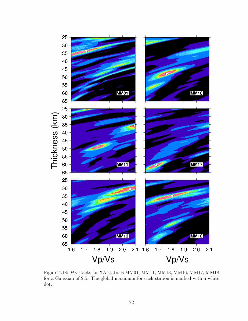
Figure 4.18: Hκ stacks for XA stations MM01, MM11, MM13, MM16, MM17, MM18for a Gaussian of 2.5. The global maximum for each station is marked with a whitedot.
72

4.9.2 Zhu and Kanamori
The Hκ stacking technique was first applied by Zhu and Kanamori (2000) to stations
in southern California (Figure 4.19). The 70 thickness results they produced are
shown in Figure 4.20 as a surface, created by averaging over 0.25× 0.25 degree bins
fitting a minimum curvature surface via the GMT surface command (Wessel and
Smith, 1991). Empty bins that are more than 0.75 degrees from a bin with data are
white. A corresponding surface using EARS results is shown in Figure 4.21. Overall
there is very good agreement, with only minor differences in the overall pattern of
crustal thickness, with perhaps the biggest difference being that EARS has access
to more stations and is able to generate results further to the northwest into central
California as well as further to the northeast in the basin and range of Nevada. These
additional stations show the thickened crust of the Sierra Nevada Mountains. Thin
crust is found near the coast and in the Saltan Sea of southernmost California.
73
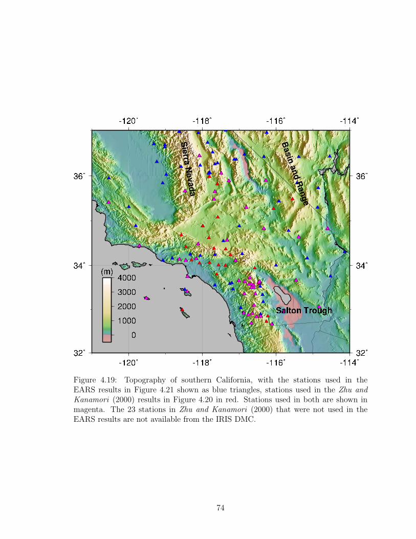
Figure 4.19: Topography of southern California, with the stations used in theEARS results in Figure 4.21 shown as blue triangles, stations used in the Zhu andKanamori (2000) results in Figure 4.20 in red. Stations used in both are shown inmagenta. The 23 stations in Zhu and Kanamori (2000) that were not used in theEARS results are not available from the IRIS DMC.
74

Figure 4.20: Crustal thickness from the 70 stations in Zhu and Kanamori (2000)shown as a minimum curvature surface after binning the stations in 0.25×0.25 degreebins. The stations used are shown as green and red triangles.
75
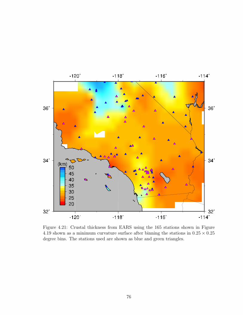
Figure 4.21: Crustal thickness from EARS using the 165 stations shown in Figure4.19 shown as a minimum curvature surface after binning the stations in 0.25× 0.25degree bins. The stations used are shown as blue and green triangles.
76

4.10 Western US
The USArray component of EarthScope is installing a temporary broadband seismic
network composed of 400 three-component broadband seismometers at a spacing of
about 70 kilometers that will roll across the United States over the course of 12
years. EARS was created with the notion of the calculation of bulk crustal properties
following USArray as it moves across the continent, with new stations being included
as they are deployed and each station’s result being updated as new data arrives.
Because the USArray deployment starts on the west coast and moves east, only the
west coast has sufficient data at this point to generate the dense results that USArray
should bring to the entire country.
The crustal thickness from EARS shows variation from 20 kilometers along the
coast to over 40 kilometers in western Washington and Oregon and the Sierras of
California, see Figure 4.22. Thinner values are seen along the coast and in southern
California with thicker values under the Sierra Nevada mountains and inland from
the Washington and Oregon coasts. The surface is created from all stations with at
least five events and where the complexity is less than 0.7. The stations thicknesses
are averaged over 0.25× 0.25 degree bins and a minimum curvature surface is fit via
the GMT surface command (Wessel and Smith, 1991). Empty bins that are more
than 0.75 degrees from a bin with data are white. This view of the EARS data allows
broad patterns of thickness to be recognized.
Perhaps the most striking feature in Figure 4.22 is the north-south trending band
of thick “crust” in western Washington and Oregon. Bostock et al. (2002) have
suggested that sepentinization of the upper mantle above the subducting Juan de
Fuca plate may obscure the signal from the base of the continental crust. This,
coupled with the ability of the Moho of the subducting oceanic slab to generate a
large signal (Owens et al., 1988), lead us to interpret this east-dipping feature as the
subducting Juan de Fuca plate. The thickness estimates from EARS agree well with
77

Figure 4.22: Unreviewed crustal thickness estimates for the western US based onaverages within 0.25× 0.25 degree bins. Empty bins that are more than 0.75 degreesfrom a bin with data are white.
78

the slab model of Fluck et al. (1997), showing the top of the slab descending from
about 20 kilometers along the coast to 50 kilometers near -123 longitude in Oregon
and Washington.
Figure 4.23: Cross section of the descending Juan de Fuca plate, modified from theresults of Bostock et al. (2002), showing the thickness estimates from EARS from 42°to45.5° latitude, with no vertical exaggeration. Stations to the west of 122.3°longitudecorrelate well with the subducting oceanic crust while stations to the east correlatewell with the continental Moho .
Figure 4.23 shows the descending Juan de Fuca plate and all EARS results between
42°to 45.5° latitude with at least 5 earthquakes and a complexity less than 0.7 overlain.
To the east, the thickness estimates agree well with a 36 kilometer thick continental
crust. Estimates to the west correlate well with the subducting oceanic crust. This
correlation continues into the area of serpentinized mantle in the forearc. The station
near the eastern edge of the forearc, TA.G04A, is more ambiguous, but is still closer
to the depth of the slab than to the continental Moho . Our technique does not yet
take dipping structures into account, and so the slope of the slab is a source of error.
Bostock et al. (2002) have also suggested that the level of sepentinization may be high
enough to invert the Moho , resulting in lower S velocities in the mantle than in the
79

overlying crust. It may be possible to identify this within the Hκ stacking technique
by looking for a minimum instead of maximum as the amplitudes of all three phases
should be inverted.
The details of these thickness maps need to be interpreted with care due to the
many possible sources of error. At each station the thickness value represents the
maximum amplitude in the Hκ stack. This value ideally should correspond to the
largest change in material properties, but this may not be true in the presence of
noise. In particular, stations with small numbers of events can often have unreliable
results. Also, the largest change in material properties may not correspond to the
base of the crust. In particular, the boundary observed in western Washington and
Oregon may correspond to the subducting slab (Bostock et al., 2002; Broucher et al.,
2003) instead of the base of the continental crust. Lastly, the surface represents an
interpolation amongst the stations, and hence is subject to lack of detail in areas
without sufficient coverage. Moreover, one outlying station can have an effect on the
surrounding areas.
It is useful to return to the individual station results to test the validity of any
feature in the surface. Figure 4.24 shows the stations that were used in the generation
of the surface in figure 4.22, aiding in the identification of outlying data points. For
example, the estimated 40 kilometer thick crust in northwestern Nevada in Figure
4.22 is unlikely to be real, and looking at the individual station results reveals that
this large value is due to a single station, TA.M08A, whose Hκ stack has a maximum
at 47 kilometers. There are eight neighboring stations, shown in Table 4.1, all of
which have thickness estimates between 29 and 37 kilometers, and so it seems likely
that this station’s result is unlikely to correspond to the true crustal thickness.
80

Figure 4.24: Stations in EARS with thickness estimates within the western US. Allstations that contributed to the surface in Figure 4.22 are shown.
81

Station Lat/Lon Thickness (km) Vp/Vs
TA.M08A 41.45/-118.38 47 km 1.69TA.L08A 42.19/-118.34 32 km 1.84TA.N08A 40.78/-118.13 31 km 1.83TA.L09A 42.02/-117.67 37 km 1.86TA.N07B 40.78/-118.97 29 km 1.81TA.L07A 42.02/-119.34 35 km 1.83TA.M09A 41.42/-117.45 35 km 1.60TA.M07A 41.39/-119.17 34 km 1.76TA.N09A 40.85/-117.52 32 km 1.77
Table 4.1: EARS results for stations near TA.M08A
82

Bibliography
Ahern, T., Data handling infrastructure at the IRIS DMC, IRIS DMC Newsletter,3 (1), 3, 2001a.
Ahern, T., What happened to FISSURES?-or-Exactly what is the data handlinginterface?, IRIS DMC Newsletter, 3 (3), 3, 2001b.
Ahern, T., Statistics: Data requests, archive size, and more, http://www.iris.edu/news/newsletter/vol8no4/index.htm, 2006.
Ahern, T., and B. Dost (Eds.), SEED Reference Manual, 3 ed., Incorporated ResearchInstitutions for Seismology, Seattle, WA, available at http://www.fdsn.org, 2006.
Ammon, C., The isolation of receiver effects from teleseismic P waveforms, Bull.,Seis. Soc. Am., 81 (6), 2504–2510, 1991.
Ammon, C., An overview of receiver-function analysis, http://eqseis.geosc.psu.edu/∼cammon/HTML/RftnDocs/rftn01.html, 1997.
Ammon, C. J., G. E. Randall, and G. Zandt, On the nonuniqueness of receiverfunction inversions, J. Geophys. Res., 95 (B10), 15,303–15,318, 1990.
Bassin, C., G. Laske, and G. Masters, The current limits of resolution for surfacewave tomography in North America, EOS Trans. AGU, 81, F897, 2000.
Bostock, M. G., R. D. Hyndman, S. Rondenay, and S. M. Peacock, An invertedcontinential Moho and serpentinization of the forearc mantle, Nature, 417, 536–538, 2002.
Box, G. E. P., and G. M. Jenkins, Time Series Analysis: Forecasting and Control,Holden-Day, San Francisco, 1976.
Bracewell, R. N., The Fourier Transform and Its Applications, McGraw-Hill, NewYork, 1978.
Broucher, T. M., T. Parsons, A. M. Trehu, C. M. Snelson, and M. A. Fisher, Seismicevidence for widespread serpentinized forearc upper manthle along the Cascadiamargin, Geology, 31, 267–270, 2003.
Buland, R., and C. H. Chapman, The computation of seismic travel times, Bull.,Seis. Soc. Am., 73 (5), 1271–1302, 1983.
83

Clayton, R., and R. Wiggins, Source shape estimation and deconvolution of teleseis-mic body waves, Geophys. J. R. Astr. Soc., 47, 151–177, 1976.
Crotwell, H., and T. Owens, Automated receiver function processing, SeismologicalResearch Letters, 76, 702–708, 2005.
Crotwell, H., and T. Owens, Automated estimation of bulk crustal properties usingUSArray data, IRIS Newsletter, 3, 4–5, 2006.
Crotwell, H. P., T. Owens, and J. Ritsema, The TauP Toolkit: Flexible seismic travel-time and ray-path utilities, Seismological Research Letters, 70, 154–160, 1999.
Davis, J. P., and I. H. Henson, User’s Guide to Xgbm: An X-Windows System tocompute Gaussian bean synthetic seismograms, Teledyne Geotech Alexandria Lab-oratories, Alexandria, VA, 1.1 ed., 1993.
Dugda, M., A. Nyblade, J. Julia, C. Langston, C. Ammon, and S. Simiyu, Crustalstructure in Ethiopia and Kenya from receiver function analysis, J. Geophys. Res.,110 (B1), doi:10.1029/2004JB003,065, 2005.
Dziewonski, A., and D. Anderson, Preliminary reference Earth model, Phys. EarthPlanet. Int., 25 (4), 297–356, 1981.
EarthScope, Exploring the structure and evolution of the north american continent,http://www.earthscope.org, 2007.
Efron, B., and R. Tibshirani, Statistical data analysis in the computer age, Science,253, 390–395, 1991.
Fluck, P., R. D. Hyndman, and K. Wang, Three-dimensional dislocation model forgreat earthquakes of the Cascadia subduction zone, J. Geophys. Res., 102 (B9),20,539–20,550, 1997.
Gilbert, F., and A. M. Dziewonski, An application of normal mode theory to theretrieval of structural parameters and source mechanisms from seismic spectra,Philisophical Transactions of the Royal Society, London A, 278, 187–269, 1975.
Gilbert, H. J., and A. F. Sheehan, Images of crustal variations in the intermountainwest, JGR, 109 (B03306), doi:10.1029/2003JB002,730, 2004.
Heal, K. M., M. L. Hansen, and K. M. Rickard, Maple V Learning Guide, Springer-Verlag, 1996.
Herrin, E., 1968 seismological tables for p phases, Bull., Seis. Soc. Am., 58 (4), 1193–1241, 1968.
Huffman, D. A., A method for the construction of minimum redundancy codes, Pro-ceedings of the IRE, 40 (9), 1098–1101, 1952.
84

Jeffreys, H., and K. E. Bullen, Seismological Tables, British Association for the Ad-vancement of Science, Burlington House, London, 1940.
Julia, J., and J. Mejıa, Thickness and vp/vs ratio variation in the Iberian crust,Geophys. J. Internat., 156, 59–72, 2004.
Kennett, B., and E. Engdahl, Traveltimes from global earthquake location and phaseidentification, Geophys. J. Internat., 105 (2), 429–465, 1991.
Kennett, B. L. N., E. R. Engdahl, and R. Buland, Constraints on seismic velocitiesin the earth from traveltimes, Geophys. J. Internat., 122, 108–124, 1995.
Langston, C., Structure under Mount Rainer, Washington, inferred from teleseismicbody waves, J. Geophys. Res., 84, 4749–4762, 1979.
Laske, G., G. Masters, and C. Reif, Crust 2.0, a new global crustal model at 2x2degrees, this is an electronic document. Date of publication: Date retrieved: March1, 2007. Date last modified: August 24, 2005, 2007.
Li, A., K. M. Fischer, S. van der Lee, and M. E. Wysession, Crust and upper mantlediscontinuity structure beneath eastern North America, J. Geophys. Res., 107 (B5),2100, doi:10.1029/2001JB000190, 2002.
Ligorrıa, J., and C. Ammon, Iterative deconvolution and receiver-function estimation,Bull., Seis. Soc. Am., 89 (5), 1395–1400, 1999.
MacKay, D. J. C., Information Theory, Inference, and Learning Algorithms, Cam-bridge University Press, 2003.
Morelli, A., and A. M. Dziewonski, Body wave traveltimes and a spherically symmet-ric P- and S-wave velocity model, Geophys. J. Internat., 112 (2), 178–194, 1993.
Owens, T., G. Zandt, and S. Taylor, Seismic evidence for an ancient rift beneath theCumberland plateau, Tennessee: A detailed analysis of broadband teleseismic pwaveforms, J. Geophys. Res., 89, 7783–7795, 1984.
Owens, T. J., R. S. Crosson, and M. A. Hendrickson, Constraints on the subduc-tion geometry beneath Western Washington from broadband teleseismic waveformmodeling, Bull., Seis. Soc. Am., 78 (3), 1319–1334, 1988.
Owens, T. J., H. P. Crotwell, C. Groves, and P. Oliver-Paul, SOD: Standing Orderfor Data, Seismological Research Letters, 75, 515–520, 2004.
Schimmel, M., and H. Paulssen, Noise reduction and detection of weak, coherentsignal through phase-weighted stacks, Geophys. J. Internat., 130, 497–505, 1997.
Tull, J. E., SAC - Seismic Analysis Code: User’s Manual, Lawrence Livermore Na-tional Laboratory, Livermore, CA, revision 2 ed., 1989.
85
Weber, M., and J. P. Davis, Evidence of a laterally variable lower mantle structurefrom P- and S-waves, Geophys. J. Internat., 102 (1), 231–255, 1990.
Wessel, P., and W. H. F. Smith, Free software helps map and display data, EOSTrans. AGU, 72 (441), http://gmt.soest.hawaii.edu, 1991.
Zandt, G., and C. J. Ammon, Continental crustal composition constrained by mea-surements of crustal poisson’s ratio, Nature, 374, 152–154, 1995.
Zhu, L., and H. Kanamori, Moho depth variation in southern California from tele-seismic receiver functions, J. Geophys. Res., 105 (B2), 2969–2980, 2000.
86