Embed Size (px)
Citation preview

AndreAs Güttler
An
dr
eA
s G
üt
tle
r
High accuracy determination of skin friction differences in an air channel flow
based on pressure drop measurements
Hig
h acc
ura
cy d
ete
rmin
atio
n o
f sk
in f
rict
ion


AndreAs Güttler
High accuracy determination of skin friction differences in an air channel flow based on pressure drop measurements

scHriftenreiHe des instituts für strömunGsmecHAnik
kArlsruHer institut für tecHnoloGie (kit)
BAnd 2

High accuracy determination of skin friction differences in an air channel flow based on pressure drop measurements
By
AndreAs Güttler

dissertation, karlsruher institut für technologie (kit)fakultät für maschinenbau, 2015
tag der mündlichen Prüfung: 18. mai 2015referenten: Prof. dr.-ing. B. frohnapfel Prof. dr.-ing. c. tropea
Print on Demand 2017 – Gedruckt auf FSC-zertifiziertem Papier
ISSN 2199-8868ISBN 978-3-7315-0502-0 DOI 10.5445/KSP/1000053260
Impressum
Karlsruher Institut für Technologie (KIT) KIT Scientific Publishing Straße am Forum 2 D-76131 Karlsruhe
KIT Scientific Publishing is a registered trademark of Karlsruhe Institute of Technology. Reprint using the book cover is not allowed.
www.ksp.kit.edu
This document – excluding the cover, pictures and graphs – is licensed under the Creative Commons Attribution-Share Alike 3.0 DE License (CC BY-SA 3.0 DE): http://creativecommons.org/licenses/by-sa/3.0/de/
The cover page is licensed under the Creative Commons Attribution-No Derivatives 3.0 DE License (CC BY-ND 3.0 DE): http://creativecommons.org/licenses/by-nd/3.0/de/

Abstract
The present work delivers a versatile, accurate and reliable wind tunnelfacility that is employed to test different flow control techniques for dragreduction in precisely adjustable test conditions. A blower wind tunnelwith a channel flow test section is developed, capable of resolving changes inthe skin friction drag as small as 0.4% thanks to the accurate measurementof both pressure drop throughout the channel and volumetric flow rate.This high accuracy is verified through a detailed uncertainty analysis andis proven by means of thoroughly conducted measurements of the smoothreference test section. A comprehensive comparison with literature datareveals the correctness of the measurements under laminar and turbulentflow conditions. The capabilities of the experimental set-up are exploited toquantify the potential skin friction reduction achievable by passive ribletsand micro grooved surfaces, as well as by active spanwise oscillating walls,each of which have been applied in the present work. The influence ofdifferent measurement strategies on the measurement accuracy is elaboratedin detail and extensively discussed.
The results of the riblet experiments are in excellent agreement with litera-ture, where the high accuracy of measurements allowed to prove the dragreduction over riblet surfaces to be independent of the streamwise length.Remarkably, the present work is the first experimental contribution in airwith comparable accuracy to that of the most accurate studies in liquids. Incontrast to existing literature, a careful analysis of the micro groove exper-iments uncovered that no effect on turbulent drag is achievable with suchdevices. This contradiction demonstrates the sensitivity of measurement ac-curacy and uncertainty estimation to the drawn conclusions. Furthermore,the capabilities of the present facility made possible to accurately quantifythe small turbulent drag reduction obtained by spanwise wall oscillationsimplemented with Dielectric Elastomer Actuators (DEA).
Finally, a new correction factor is proposed in so as to account for threedimensional effects, such as finite channel width and corresponding flow

ii Abstract
development issues. It is hypothesized that this factor significantly improvesthe comparability of drag reduction results from numerical channel flowsimulations and experimental studies of varying test-section aspect ratio.

Kurzfassung
Die vorliegende experimentelle Arbeit liefert eine vielseitige, prazise undzuverlassige Windkanalanlage zur Untersuchung verschiedener Technikender Stromungskontrolle zur Reibungsminderung unter gleichen Testbedin-gungen. Ein Blaswindkanal mit einer Kanalmessstrecke wird entwickelt,dem genauste Messtechnik zur Bestimmung des Druckabfalls entlang derMessstrecke sowie des Volumenstroms erlaubt, feinste Wandreibungsdif-ferenzen von 0.4% aufzulosen. Diese hohe Genauigkeit wird verifiziertdurch eine detailierte Fehleranalyse und anhand sorgfaltig durchgefuhrterMessungen der glatten Referenzmessstrecke bestatigt. Ein umfangreicherVergleich mit Literaturdaten belegt die Richtigkeit der Messergebnisse unterlaminaren und turbulenten Stromungsbedingungen. Die Fahigkeiten desexperimentellen Aufbaus werden genutzt, um Reibungsminderung verschie-dener Techniken zur Stromungskontrolle zu quantifizieren, durch passiveRiblet- und Microgroovesoberflachen sowie mittels aktiver oszillierenderWande, die alle in dieser Arbeit zur Anwendung kamen. Die Auswirkungverschiedener Messstrategien auf die Messgenauigkeit wird im Detail erar-beitet und ausfuhrlich diskutiert.
Die Ergebnisse der Ribletexperimente zeigen eine exzellente Ubereinstim-mung mit Literaturwerten, wobei die hohe Messgenauigkeit die Bestatigungder Unabhangigkeit der Reibungsreduktion uber Ribletflachen von derstromweitigen Position erlaubt. Bemerkenswerter Weise gelingt mit dervorliegenden Arbeit der erste experimentelle Beitrag in einer Luftstromung,der eine vergleichbare Messgenauigkeit wie die genausten Untersuchungenin Flussigkeiten erzielt. Im Gegensatz zur existierenden Literatur deckteine sorgfaltige Analyse der Microgrooves auf, dass mit diesen keine Bee-influßung der turbulenten Reibung erzielt wird. Dieser Gegensatz zeigtdie Sensibilitat der Messgenauigkeit und Fehlerabschatzung auf die gezo-genen Schlusse. Außerdem ermoglicht die Anlage die geringe turbulenteReibungsminderung, die mit spannweitig oszillierenden Wanden, die mit-tels dielektrischer Elastomeraktuatoren (DEA) umgesetzt wurde, genau zuquantifizieren.

iv Kurzfassung
Daruber hinaus wird ein Korrekturfaktor vorgeschlagen, um dreidimen-sionale Effekte, wie begrenzte die Kanalbreite und die daraus resultierendeAusbildung der Kanalstromung zu berucksichtigen. Es wird angenommen,dass dieser Faktor zu einer deutlichen Verbesserung der Vergleichbarkeitder Reibungsminderungsergebnisse von numerischen Untersuchungen vonKanalstromungen zu experimentellen in Abhangigkeit des Seitenverhalt-nisses des Kanals fuhrt.

Contents
Abstract i
Kurzfassung iii
Table of Contents viii
1 Introduction 1
2 Fundamentals of air channel flows 92.1 Analytical consideration of a channel flow . . . . . . . . . . 9
2.1.1 Laminar channel flow . . . . . . . . . . . . . . . . . 112.1.2 Turbulent channel flow . . . . . . . . . . . . . . . . . 15
2.2 Examination of the initial assumptions for ideal channel flow 202.2.1 Concept of hydraulically smooth walls . . . . . . . . 212.2.2 Flow development . . . . . . . . . . . . . . . . . . . 242.2.3 Approximation of two-dimensionality . . . . . . . . . 27
2.3 Properties of air . . . . . . . . . . . . . . . . . . . . . . . . 32
3 Experimental setup 373.1 Wind tunnel . . . . . . . . . . . . . . . . . . . . . . . . . . . 37
3.1.1 Radial ventilator . . . . . . . . . . . . . . . . . . . . 393.1.2 Settling chamber . . . . . . . . . . . . . . . . . . . . 403.1.3 Flow rate measurement . . . . . . . . . . . . . . . . 423.1.4 Wind tunnel control . . . . . . . . . . . . . . . . . . 46
3.2 Test section . . . . . . . . . . . . . . . . . . . . . . . . . . . 473.3 Measurement instrumentation . . . . . . . . . . . . . . . . . 51
4 Measurement uncertainty 554.1 Modus operandi . . . . . . . . . . . . . . . . . . . . . . . . 554.2 Flow rate measurement . . . . . . . . . . . . . . . . . . . . 58
4.2.1 Ambient quantities . . . . . . . . . . . . . . . . . . . 584.2.2 Uncertainty of the differential pressure measurement
for flow rate determination . . . . . . . . . . . . . . 60
vi Contents
4.2.3 Fabrication tolerances . . . . . . . . . . . . . . . . . 624.2.4 Uncertainty of the calibration parameters . . . . . . 634.2.5 Combined uncertainty of flow rate measurement . . 634.2.6 Uncertainty of Reynolds number in the test section . 65
4.3 Determination of pressure drop along the test section . . . . 694.3.1 Uncertainty of friction coefficient . . . . . . . . . . . 714.3.2 Determination of skin friction changes in dependence
of the measurement strategy . . . . . . . . . . . . . 734.4 Steadiness of the flow . . . . . . . . . . . . . . . . . . . . . 76
5 Reference measurement 795.1 Naturally developing flow . . . . . . . . . . . . . . . . . . . 805.2 Artificially generated turbulent flow . . . . . . . . . . . . . 875.3 Impact of the laboratory environment on the flow development 935.4 Two-dimensionality of the flow . . . . . . . . . . . . . . . . 96
5.4.1 Pitot tube measurement . . . . . . . . . . . . . . . . 975.4.2 Preston tube measurement . . . . . . . . . . . . . . 1005.4.3 Influence of three-dimensional effects . . . . . . . . . 1035.4.4 Summary of the reference measurements . . . . . . . 107
6 Riblets 1096.1 Introduction . . . . . . . . . . . . . . . . . . . . . . . . . . . 1096.2 Physical principle . . . . . . . . . . . . . . . . . . . . . . . . 1106.3 Experimental study of riblets . . . . . . . . . . . . . . . . . 116
6.3.1 Experimental investigation - State-of-the-art . . . . 1166.3.2 Design and fabrication of the structures . . . . . . . 1176.3.3 Focus of the experimental investigations . . . . . . . 1196.3.4 Arrangement of experimental setup . . . . . . . . . . 120
6.4 Discussion of the results . . . . . . . . . . . . . . . . . . . . 1216.4.1 Strategy to determine the skin friction change . . . . 1266.4.2 Change of the skin friction drag . . . . . . . . . . . . 1296.4.3 Influence of spanwise velocity distribution . . . . . . 131
6.5 Conclusions . . . . . . . . . . . . . . . . . . . . . . . . . . . 134
7 Micro grooves 1357.1 Statistical consideration of turbulence via invariant map . . 136
7.1.1 Examination of skin friction reduction with respectto the anisotropy of turbulence . . . . . . . . . . . . 138
7.2 Micro grooves - State-of-the-art . . . . . . . . . . . . . . . . 1417.2.1 Basic idea of micro grooves . . . . . . . . . . . . . . 141

Contents vii
7.2.2 Previous results for grooved surfaces in turbulent flows 1437.2.3 Previous results for grooved surfaces in
transitional flows . . . . . . . . . . . . . . . . . . . . 1477.3 Experimental investigation of micro grooves . . . . . . . . . 149
7.3.1 Fabrication of the groove structures . . . . . . . . . 1507.3.2 Measurement strategy . . . . . . . . . . . . . . . . . 151
7.4 Measurements in turbulent flow . . . . . . . . . . . . . . . . 1517.4.1 Discussion of results in turbulent channel flow . . . . 153
7.5 Measurements in transitional flow . . . . . . . . . . . . . . . 1577.5.1 Discussion of transitional results in transitional
channel flow . . . . . . . . . . . . . . . . . . . . . . 161
8 Spanwise oscillating walls implemented via dielectricelastomer actuators 1658.1 Spanwise oscillating walls . . . . . . . . . . . . . . . . . . . 166
8.1.1 Dielectric electroactive polymers . . . . . . . . . . . 1688.1.2 Working principle of dielectric elastomer actuators . 1698.1.3 Arrangement of experimental set-up . . . . . . . . . 1718.1.4 Measurement strategy . . . . . . . . . . . . . . . . . 174
8.2 Measurement results . . . . . . . . . . . . . . . . . . . . . . 1758.2.1 Measurement of reference case . . . . . . . . . . . . 1758.2.2 DEA in opposite wall configuration . . . . . . . . . . 1768.2.3 DEA in cascaded configuration . . . . . . . . . . . . 1808.2.4 Influence of limited spanwise actuator length on
skin friction reduction . . . . . . . . . . . . . . . . . 1818.3 Discussion of the DEA results . . . . . . . . . . . . . . . . . 182
9 Summary and conclusions 1839.1 Comparability of experimental and numerical data . . . . . 1859.2 Riblets . . . . . . . . . . . . . . . . . . . . . . . . . . . . . . 1869.3 Microgrooves . . . . . . . . . . . . . . . . . . . . . . . . . . 1879.4 Dielectric elastomer actuators . . . . . . . . . . . . . . . . . 189
10 Outlook 19110.1 Prospects of the facility . . . . . . . . . . . . . . . . . . . . 19110.2 Studies of channel flow . . . . . . . . . . . . . . . . . . . . . 19210.3 Channel flow studies at high Re . . . . . . . . . . . . . . . . 194
Bibliography 195
.

viii Contents
List of Figures 214
List of Tables 215
A Appendix 217A.1 Extension of the operation range to small flow rates for
inlet nozzles . . . . . . . . . . . . . . . . . . . . . . . . . . . 217A.2 Determination of the turbulence intensity without
velocity calibration . . . . . . . . . . . . . . . . . . . . . . . 220
1 Introduction
Interactions between fluids and surfaces play an essential role in manynatural and industrial flows. In almost all technical flow processes skinfriction at solid walls creates undesirable energy losses. During the lastdecades technological advances inspired the investigation of strategies aimedat manipulating the characteristics of fluid flows to minimize energy losses.Due to the potential energy savings, flow control nowadays represents amajor topic of modern fluid mechanics (Gad-el Hak, 2000). One main goalof flow control is the reduction of skin friction in internal and externalflows. Many strategies have been developed to achieve this goal based onthe existence of two fundamental flow states:
Already in his pioneering work Osborne Reynolds (1883) observed twodifferent forms of flow in a pipe, which he described according to thecomplexity of their movement as “direct” and “sinuous”. The occurrenceof either of these flow states, nowadays called laminar and turbulent re-spectively, depends on a dimensionless quantity first proposed by Stokes(1851), which has later been named after Osborne Reynolds. This so-calledReynolds number 𝑅𝑒 combines the flow velocity 𝑈 , the kinematic viscosity𝜈 of the fluid and a characteristic length 𝐿 - which in case of a pipe flow isthe diameter 𝐷 - as follows:
𝑅𝑒 = 𝑈𝐿
𝜈. (1.1)
Reynolds found out that above a critical value of this number the flowtransitioned from the laminar to the turbulent state and that the latterstate is characterized by significantly higher wall friction: “The resistanceis generally proportional to the square of the velocity (turbulent) [· · · ] andproportional to the velocity”, if it is laminar (Reynolds, 1883).
Reynolds observed that the higher momentum exchange associated withturbulent flow causes fluid elements to “eddy about in sinuous paths”, whilein the laminar state they move “along direct lines”, which explains thehigher drag in the former. This observation constitutes the rationale of
2 1 Introduction
scientific research in the field of drag reduction: the manipulation of thefriction intensive turbulent flow state. Two strategies of flow control in thefield of drag reduction are deduced:
⇒ the sustainment of a laminar flow state at higher values of 𝑅𝑒, forwhich the flow would be otherwise naturally turbulent;
⇒ a modification of the turbulent regime aimed to reduce the excessturbulent skin-friction drag.
Based on these strategies various approaches to reduce the friction draghave been developed. A differentiation of the methods can be made byclassifying them into active - those consuming energy - and passive - thosenot utilizing external energy sources. While active techniques - mainly ininteraction with complex feedback control systems - promise applicability inwide velocity ranges and high amounts of savings, methods based on passiveprinciple score with efficiency and simplicity in operation. In spite of thelarge number of research projects devoted to the subject, only few flowcontrol strategies developed to a state enabling application in laboratoryexperiments. In the following promising approaches for passive and activeflow control methods are exemplarily presented.
One of the most famous examples for a passive method are riblets. Theseshark-skin like structures have been studied for more than three decadesand their capabilities in reducing drag in a turbulent flow have beendemonstrated (Bechert et al., 1997; Lee & Lee, 2001; Walsh, 1982). Thestandard type of two-dimensional fin structures has been extensively studiedexperimentally. The effectiveness of riblets strongly depends on 𝑅𝑒 with arelatively small drag reduction of typically 4-10%.
The most successful application of skin friction drag reduction is alsorepresented by a passive method (Toms, 1948): the addition of foreignsubstances to fluid flows, for example polymers with a long-chain structure.Despite a very low concentration of few ppm the polymers have shown theoutstanding reduction, up to 80%, in turbulent flows (Lumley & Kobu,1985). Such additives are used in the Transalaska pipeline for oil transportsince 1979.
Micro grooves are a recently proposed passive technique suggested forturbulent drag reduction, that also showed promising results in transitiondelay (Jovanovic et al., 2010a). These streamwise aligned grooves are of verysmall dimensions -significantly smaller than riblets- and their fabricationis a problem to be solved. Groove structures were found to yield a high

3
amount of skin friction drag reduction but only for narrow range of 𝑅𝑒(Frohnapfel et al., 2007a).
A comprehensive review on the actuator design for active flow control isprovided by Cattafesta & Sheplak (2011). An example for an active flowcontrol aimed at delaying laminar to turbulent transition, which has beenin focus in the recent years, is boundary layer stabilization with plasmaactuators. Its working principle is based on ionization and acceleration ofair molecules, where the major advantage is the fast response time andthe absence of any moving parts. A small wall jet is generated, which canbe used to import momentum into the boundary layer (Duchmann et al.,2013) or damp distortions, which trigger the transition process (Kurz et al.,2013).
Spanwise wall forcing is an active, predetermined flow control techniquefor turbulent skin-friction drag reduction which can achieve high-values ofdrag reduction. It has been intensively studied numerically (Quadrio &Ricco, 2004) and has been given experimental verification (see, for exampleRicco & Wu (2004)). Its simplest implementation is the oscillating wall, inwhich a portion of the wall wetted by the fluid exhibits in-plane oscillationsperpendicular to the mean flow direction. In spite of its simplicity, designinga device capable of mimicking this movement, which contemporaneouslymeets the space- and timescales of wall turbulence and is energeticallyefficient, is a very challenging task.
The few flow control strategies, which developed to a state enabling ap-plication in laboratory experiments, usually achieved a skin-friction dragreduction of less than 10%. At the fairly low values of the Reynolds number,for which laboratory implementation of turbulent flow control is possible,skin-friction forces can be very low. The relatively small variation of dragcreated by the control is therefore very difficult to detect. Additionallymany parameters influencing the flow properties need to be kept constantto ensure reproducible results, e.g. the arrangement of set-up, the fluidparameters and the environmental influence, etc.. The different researchobjectives comprising laminar, transitional or turbulent flow for the vari-ety of studies led to different designs of the corresponding experimentalfacilities.
In summary, the boundary conditions and uncertainties of measurementdiffer to such an extent, that a comparative evaluation of the methods inrespect to the amount of drag reduction or efficiency is rarely possible. Themajor goal of the present work, is therefore is to provide an experimental
1 Introduction

4 1 Introduction
facility for high accurate quantification of various methods of flow controlunder identical reproducibility conditions. Thus, a number of far reachingdecisions needs to be made for the basic design of experimental set-up.
A fundamental decision for experimental investigations is the choice ofthe working medium. In many experimental studies, for instance in ribletresearch, liquids like commonly water or oil (Bechert et al., 1997) insteadof air are used as working fluid. Larger physical dimensions of the usuallyvery small flow control devices exhibit advantages in manufacturing andlarger friction forces are easier to be measured accurately in similar flowscenarios. This principle led to excellent accuracy in the case of the oiltunnel in Berlin (Bechert et al., 1992).
The choice of the fluid influences the kind of drag reduction principles whichcan be investigated. Some of the drag reduction techniques are bound toliquid media such as long-chain polymers injection, which is not applicablein an air flow. In the same way the appliance of other flow control methodsis limited to gaseous media. The aforementioned plasma actuator, forinstance, ionizes gas molecules to produce a near-wall body force (Moreau,2007) and is thus bound to the gaseous state. Also dielectric elastomeractuators (DEA) (Gouder (2011), Gatti (2014b)), tested in the context ofthe present work, cannot sustain the fluiddynamic and body forces in waterflow, where the electric isolation is also problematic. Hence, certain flowcontrol methods being of interest for the present investigation cannot beoperated in liquids. Furthermore, air flow offers substantial advantages ifthe major problems of miniaturization and measurement accuracy can beresolved. In particular, the handling of a wind tunnel is simpler and lessextensive maintenance is required in comparison to an oil or water tunnelfacility.
In summary, there is valid reason to run experiments in air flow. However,the high accuracy determination of extremely small difference in the wallshear stress represents the challenging task of the present work.
Further, the type of investigated flow has a significant influence on thedesign of the facility and even on the appropriate measurement technique.There are three classical cases for experimental investigations of wall bound-ed flows: constant pressure boundary layer, pipe flow and channel flow(Schultz & Flack, 2013). While the boundary layer flow is characterizedby a continuous development in the streamwise direction, both inner flowsreach a fully developed state after a certain running length. This simplifiesthe reproduction of a flow in different experiments and facilities and hence

5
their comparability. Constant pressure boundary layer at very controlledconditions as required in aerodynamic experimental investigations are moredifficult to reproduce, which results in a limited measurement accuracy(Marusic et al., 2010). Another crucial aspect is the need for detecting vari-ations in the wall friction smaller than one percent. Oil film interferometry,which represents the most accurate technique available in zero pressuregradient boundary flow is generally specified with (±1 − 2%) (Marusicet al., 2010). In addition the application of the oil film interferometryis constricted to smooth surfaces and thus not able to comply with thespectrum of interest for the research of the present work, which includesmodifications of surface morphology.
However, studies in fully developed pipe and channel flows offer a precisedetermination of wall friction via pressure drop measurements along thelength of a pipe or channel and the advantageous situation of extensiveexperimental (e.g. Dean (1978); Durst et al. (1998); Huebscher (1947);Monty (2005); Nikuradse (1932)) as well as numerical studies (Eggels et al.(1994); Jimenez et al. (2010); Kim et al. (1987); Moin & Mahesh (1998))-for the laminar case even analytical results (cf. Chapter 2) - that can befound in the literature (Schlichting, 1959; Spurk & Aksel, 2006).
The choice of a channel flow experiment in the present study enablescomparison with numerical investigations of turbulent flow control. Ina plenty of Direct Numeric Simulations (DNS) the convenient boundaryconditions of such a quasi two-dimensional flow are chosen to economizecomputational effort. While the DNS provides a deep insight into detailsof the flow structures, experimental investigations can easily run extensiveparameter studies. In ideal case numerical and experimental investigationswork hand in hand to combine benefits and potentials of both approaches.From the experimental side a simple, but practical reason leads to preferworking in a channel: most techniques for flow control are complicated toapply on a curved surface of a pipe.
The 2D-channel flow is itself of minor interest for direct use in engineeringapplication, but it serves as the key interface between the numerical andanalytical research and the experimental studies. Additionally it exhibitsfavorable boundary conditions for all three disciplines of the research.Numerous experimental studies of riblets have proved that results froma channel flow (Bechert et al., 1997; Gruneberger & Hage, 2011; Walsh,1982) can be transferred to a boundary layer flow for turbulent conditions(Viswanath, 2002).
1 Introduction

6 1 Introduction
In summary, pressure drop measurements in channel flow allow high accu-racy determination of skin-friction, containing precise information aboutchanges in the wall friction and enabling to directly compare different tech-niques. These fundamental decisions on the experimental concept prescribethe approach taken in the present study.
In the first step an experimental facility is designed and built upon this basicconcept, while in the second step it needs to be thoroughly verified, thatthis experimental set-up holds the expectations in measurement accuracy.Subsequently, application of selected active and passive techniques for skinfriction reduction is to be demonstrated. Hence, the major goals of thepresent work can be formulated as follows:
Part I : Develop a platform to study and compare different techniques toreduce skin friction drag under the constraints of:
∙ accurate determination of skin friction based on the concept ofpressure drop measurement in a channel flow
∙ applicability of active and passive control techniques
∙ ability to operate in laminar, transitional and turbulent flowconditions, while focusing on the latter
∙ flow medium air
∙ wide range of Reynolds number 𝑅𝑒.
Part II : Demonstrate the capabilities of the set-up in comparison to liter-ature data for a hydraulically smooth surface.
Part III: Show the applicability of active and passive techniques and en-able new insight into previously investigated skin friction reducingapproaches:
∙ riblets
∙ micro grooves
∙ spanwise wall oscillation
The riblet study has two goals. On the one hand the agreement to literaturedata can demonstrate the reliability of data generated in the facility of thepresent study. On the other hand the choice of air as working fluid allowsto shed light on spatial transients, thanks to the longer running lengthcompared to what is usually achieved in oil channels.
7
The few experimental as well as numerical studies on the topic of microgrooves leave room for various follow-up questions such as: Which is theoptimal geometry? How does the optimal structure size scale with 𝑅𝑒? Isit possible to extend the effective Reynolds number range? Additionallythe micro grooves have been tested in transitional flows (Jovanovic et al.,2011), where further examination is required.
The key question regarding wall oscillations is how to efficiently implementthe wall movement. The present facility turned out to be a very convenienttest rig for the novel approach of dielectric electroactive polymers, thathave been mechanically characterized and numerically studied by Gattiet al. (2014). In comparison to numerical simulations, the small surfacearea covered by the available actuators leads to very small differences inthe skin friction. For the experimental set-up the challenge is to obtain ameasurement accuracy which is high enough to well resolve the possiblyvery small variations of the skin friction drag.
The structure of this thesis is organized as follows:
In the first part the concept of the set-up will be developed from a theoreticalstandpoint. Subsequently, the implemented experimental set-up will beverified by data comparison with literature references. Therefore Chapter 2introduces the fundamentals of a channel flow from analytical as well as fromexperimental side and adds numerical input where helpful. Additionally theessential properties of air are introduced. The following Chapter 3 arguesthe construction of the experimental set-up divided into the wind tunneland the channel test section. The description of the set-up is completedwith the introduction of the measurement instrumentation. In Chapter 4a very thorough discussion of uncertainty estimation and correspondingerror propagation is presented, which is of utmost importance for suchhigh accuracy measurements. The measurement results of the channel withsmooth walls are compared to literature data for fully turbulent and laminar-transitional flow in Chapter 5. Chapters 6, 7 and 8 discuss the concepts, theapplication to the channel experiment and present the measurement resultsof three different approaches for turbulent drag reduction: by passive meansriblets (Chap. 6) as well as micro grooves (Chap. 7) and active representedby oscillating walls, implemented with novel type of dielectric electroactivepolymer actuators (Chap. 8). The investigations are completed with astudy of micro grooves in the transitional regime.
1 Introduction
To the reader’s convenience, the experimental studies for each flow controltechnique are written as self-contained reports.


2 Fundamentals ofair channel flows
This Chapter introduces the fundamentals of channel flows from an experi-mental point of view. The Chapter starts with the definition of an idealchannel flow. On this basis analytical considerations of the channel flowwill be made for turbulent as well as laminar flow conditions. Limitations ofthis approach due to the idealized boundary conditions are mentioned andthe measurement principle for the determination of the wall shear stress isdeduced. Additionally, the relevant properties of the fluid are discussed.The consideration is completed by the presentation of experimental andsome numerical results characteristically observed in channel flows.
2.1 Analytical consideration of a channel flow
For analytical considerations a channel flow is defined as a steady flow inbetween two parallel plates of a distance 𝐻. The hypothesis is made thatthe plates are infinitely in length and width. In consequence the flow can beconsidered two-dimensional due to the infinite width and independent fromthe streamwise position due to the infinite length. Thus we can formulatefollowing assumptions:
⇒ the two-dimensionality of the flow field
⇒ a fully developed flow state
⇒ bounding walls are perfectly smooth
With regard to the experimental studies in air two more simplificationsconcerning the properties of the fluid are made:
10 2 Fundamentals of air channel flows
⇒ for the low subsonic wind speeds of the present study the flow istreated incompressible. Furthermore even the density is assumed tobe constant.
⇒ additionally air is assumed to be an ideal Newtonian fluid
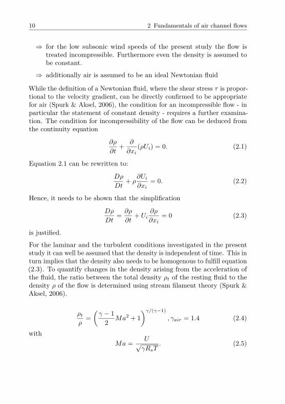
While the definition of a Newtonian fluid, where the shear stress 𝜏 is propor-tional to the velocity gradient, can be directly confirmed to be appropriatefor air (Spurk & Aksel, 2006), the condition for an incompressible flow - inparticular the statement of constant density - requires a further examina-tion. The condition for incompressibility of the flow can be deduced fromthe continuity equation
𝜕𝜌
𝜕𝑡+ 𝜕
𝜕𝑥𝑖(𝜌𝑈𝑖) = 0. (2.1)
Equation 2.1 can be rewritten to:
𝐷𝜌
𝐷𝑡+ 𝜌
𝜕𝑈𝑖
𝜕𝑥𝑖= 0. (2.2)
Hence, it needs to be shown that the simplification
𝐷𝜌
𝐷𝑡= 𝜕𝜌
𝜕𝑡+ 𝑈𝑖
𝜕𝜌
𝜕𝑥𝑖= 0 (2.3)
is justified.
For the laminar and the turbulent conditions investigated in the presentstudy it can well be assumed that the density is independent of time. This inturn implies that the density also needs to be homogenous to fulfill equation(2.3). To quantify changes in the density arising from the acceleration ofthe fluid, the ratio between the total density 𝜌𝑡 of the resting fluid to thedensity 𝜌 of the flow is determined using stream filament theory (Spurk &Aksel, 2006).
𝜌𝑡
𝜌=
(𝛾 − 1
2 𝑀𝑎2 + 1)𝛾/(𝛾−1)
, 𝛾𝑎𝑖𝑟 = 1.4 (2.4)
with𝑀𝑎 = 𝑈√
𝛾𝑅𝑠𝑇. (2.5)

2.1 Analytical consideration of a channel flow 11
If the static flow quantities are altered due to motion of the fluid such,that the effect is not negligible for the determination of the air density,a Mach-number of 𝑀𝑎 > 0.2 is practically necessary. This means that amaximum deviation from the density of resting air of 2% is tolerated (Pope& Harper (1966) define even 300miles/h). In the present investigationthe Mach number is limited to 𝑀𝑎 < 0.045. Compressibility effects staybelow 0.1% even for the highest 𝑅𝑒. Therefore, the flow can be treatedincompressible in very good approximation without any influence of thequality of the results. This still does not mean that the applicability of theassumption of constant density is valid. For the very accurate measure-ments in the present study even smallest changes of the static pressure andtemperature through the channel can influence the measurement results,which is further examined in Chapter 4.
In the following the flow through a channel is discussed based on analyticalconsiderations for laminar and turbulent conditions. Later on, limitationson the applicability of the remaining three assumptions for the experimentwill be introduced step by step.
2.1.1 Laminar channel flow
Figure 2.1: Definition of a channel
In the case of a fully developed laminar channel flow between two platesof distance 𝐻, as it is shown in Figure 2.1, an analytical solution for thevelocity profile and hence the skin friction coefficient 𝑐𝑓 can be derived fromthe Navier-Stokes equation. For an incompressible fluid the Navier-Stokesequations write:
𝜌
(𝜕𝑈𝑗
𝜕𝑡+ 𝑈𝑖
𝜕𝑈𝑗
𝜕𝑥𝑖
)= − 𝜕𝑝
𝜕𝑥𝑗+ 𝜂
𝜕2𝑈𝑗
𝜕𝑥𝑖𝜕𝑥𝑖+ 𝜌𝑔𝑗 (2.6)

12 2 Fundamentals of air channel flows
In a steady air flow all derivatives in time vanish. The flow direction is ina horizontal plane and hydrostatic forces due to gravity are assumed to benegligible.
𝜕𝑈𝑗
𝜕𝑡= 0 (2.7)
In a two-dimensional, incompressible flow the continuity equation writes:
𝜕𝑈1
𝜕𝑥1+ 𝜕𝑈2
𝜕𝑥2= 0 (2.8)
Derivatives of 𝑈 in 𝑥1-direction vanish for a fully developed flow. With theboundary condition at the wall 𝑈2(𝑥 = 𝐻
2 ) = 0 we obtain
𝑈2 = const. = 0. (2.9)
The Navier-Stokes equations for the 𝑥2-direction writes
0 = − 𝜕𝑝
𝜕𝑥2⇔ 𝑝 = 𝑝(𝑥1). (2.10)
Thus the pressure is constant over a cross sectional plane at arbitraryposition in the channel.The 𝑥1-component of the Navier-Stokes equations simplifies to:
0 = − 𝜕𝑝
𝜕𝑥1+ 𝜂
𝜕2𝑈1
𝜕𝑥2𝜕𝑥2(2.11)
This differential equation is solved integrating two times in 𝑥2. By doingso, two unknown constants 𝐶1 and 𝐶2 are obtained, whose determinationsucceeds concerning the constraints at the wall
𝑈1(𝑥2= 𝐻2 ) = 𝑈1(𝑥2=− 𝐻
2 ) = 0. (2.12)

2.1 Analytical consideration of a channel flow 13
This enables to determine the flow velocity 𝑈1 in streamwise direction independence on the channel height H, yielding to a parabolic shape of thevelocity profile as shown in Figure 2.2.
𝑈1 = 12𝜂
(− d𝑝
d𝑥1
) (𝐻2
4 − 𝑥22
)(2.13)
The velocity at the centerline 𝑈𝑐 writes:
𝑈𝑐 = 𝑈1(𝑥2=0) = 12𝜂
(− d𝑝
d𝑥1
) (𝐻2
4
). (2.14)
Figure 2.2: Parabolic velocity profile in a laminar channel flow
Now, the wall shear stress 𝜏𝑤 is introduced as
𝜏𝑤 = 𝜂𝑑𝑈1
𝑑𝑥2
𝑥2=− 𝐻
2
. (2.15)
By differentiating equation (2.14) with respect to 𝑥2 and evaluating at thewall 𝑥2 = − 𝐻
2 we derive
𝑑𝑈1
𝑑𝑥2
𝑥2=− 𝐻
2
= 1𝜂
d𝑝
d𝑥1
𝐻
2 (2.16)
and find the relation between the pressure drop and the wall shear stress
𝜏𝑤 = −𝐻
2d𝑝
d𝑥1. (2.17)
Inserting this result in 2.14 allows to calculate the mean velocity 𝑈𝑏
(𝑏=bulk)

14 2 Fundamentals of air channel flows
𝑈𝑏 = 2𝐻
∫ 𝐻2
0𝑈1d𝑥2 = 2
𝐻
12𝜂
(2𝜏𝑤
𝐻
) ∫ 𝐻2
0
(𝐻2
4 − 𝑥22
)d𝑥2
= 2𝐻𝜏𝑤
𝜂
112 = 2
3𝑈𝑐
(2.18)
The skin-friction coefficient 𝑐𝑓 is introduced by normalizing the wall shearstress with the kinetic energy of the bulk flow.
𝑐𝑓 = 𝜏𝑤𝜌2 𝑈2
𝑏
= 𝜏𝑤𝜌2 (2𝐻 𝜏𝑤
𝜂1
12 )𝑈𝑏
= 12𝜂
𝜌𝑈𝑏𝐻= 12𝜈
𝑈𝑏𝐻(2.19)
In the above equation the analytical results for 𝜏𝑤 (Eq. (2.17)) and 𝑈𝑏 (Eq.(2.18)) in laminar channel flow have been used.
If we choose the channel height 𝐻 as characteristic length to define theReynolds number,
𝑅𝑒 = 𝑈𝑏 𝐻
𝜈(2.20)
we get the simple expression for 𝑐𝑓
𝑐𝑓 = 12𝑅𝑒𝑏
. (2.21)
In fully developed channel flow the differential d𝑝/d𝑥1 is constant and thusequal to the quotient of Δ𝑝 and a length Δ𝑥1. Considering the pressuredifference Δ𝑝 over a run length 𝑙, we can rearrange equation (2.17) andinsert the expression we obtained for 𝑐𝑓 in Eq. (2.21)
Δ𝑝 = 2𝜏𝑤𝑙
𝐻= 12
𝑅𝑒
𝑙
𝐻𝜌𝑈2
𝑏 . (2.22)
With this analytical expression for the pressure difference over a definedrunning length 𝑙, the resulting wall friction can be calculated for Reynoldsnumbers corresponding to the laminar flow state.

2.1 Analytical consideration of a channel flow 15
2.1.2 Turbulent channel flow
In turbulent flow we can assume the flow to be statistically steady and thefluctuations in all directions superposed to the mean quantities. Thus it isconvenient to split the velocity in two components: A time-averaged meanvalue �� and a fluctuation 𝑢.
Using this decomposition in equation (2.7) and (2.6) and time-averaging ofthe term yields the Reynolds-averaged equations (Pope, 2000) for continu-ity
𝜕𝑈𝑖
𝜕𝑥𝑖= 0 (2.23)
and momentum
𝜕𝑈𝑗
𝜕𝑡+ 𝑈𝑖
𝜕𝑈𝑗
𝜕𝑥𝑖= −1
𝜌
𝜕𝑝
𝜕𝑥𝑗+ 𝜈
𝜕2𝑈𝑗
𝜕𝑥𝑖𝜕𝑥𝑖− 𝜕𝑢𝑖𝑢𝑗
𝜕𝑥𝑖(2.24)
in incompressible flow. Here, the last term describes the Reynolds stressescaused by the turbulent fluctuations. Now we follow the same procedure asused for the laminar flow and write the continuity equation for the meanquantities.
𝜕𝑈1
𝜕𝑥1+ 𝜕𝑈2
𝜕𝑥2= 0 (2.25)
For a fully developed flow 𝜕𝑈1𝜕𝑥1
=0 we obtain
𝜕𝑈2
𝜕𝑥2= 0 ⇒ 𝑈2 = const = 0. (2.26)
With this result for 𝑈2 for wall-normal direction and the assumption ofa statistically stationary and fully developed flow the second componentsimplifies to
0 = −1𝜌
𝜕𝑝
𝜕𝑥2− 𝜕𝑢2𝑢2
𝜕𝑥2. (2.27)

16 2 Fundamentals of air channel flows
Contrary to laminar flow we do not obtain a constant pressure over a crosssection due to the additional stress term. We integrate 2.27 and determinethe resulting constant defining the mean pressure at the top wall 𝑝𝑤 =𝑝(𝑥1, 𝐻
2 ) and insert the boundary condition at the wall 𝑢22(𝑥2= 𝐻
2 ) = 0:
𝑢2𝑢2 + 𝑝
𝜌= 𝑝𝑤(𝑥1)
𝜌(2.28)
Differentiating in 𝑥1-direction yields, that the mean axial pressure gradientis uniform across the flow.
𝜕𝑝
𝜕𝑥1= 𝜕𝑝𝑤
𝜕𝑥1(2.29)
Now we write the 𝑥1-component of the Navier-Stokes equations with theassumptions mentioned before:
0 = −1𝜌
𝜕𝑝
𝜕𝑥1+ 𝜈
𝜕2𝑈1
𝜕𝑥2𝜕𝑥2− 𝜕𝑢1𝑢2
𝜕𝑥2(2.30)
In contrast to the laminar case the problem is not analytically solvable. Ifwe follow Pope (2000) and rewrite the equation using the expression forthe total stress
𝜏 = 𝜌𝜈d𝑈1
d𝑥2− 𝜌(𝑢1𝑢2) (2.31)
we obtain
𝜕𝜏
𝜕𝑥2= 𝜕𝑝𝑤
𝜕𝑥1. (2.32)
and find the gradient of normal stress balanced with the gradient of thetotal stress in 𝑥2-direction.
The integration of equation (2.30) over half of the channel height 𝐻/2 withthe total shear stress being zero for 𝑥2 = 𝐻/2 yields:
2.1 Analytical consideration of a channel flow 17
0 = −∫ 𝐻
2
0
1𝜌
𝜕𝑝
𝜕𝑥1d𝑥2 +
∫ 𝐻2
0𝜈
𝜕2𝑈1
𝜕𝑥2𝜕𝑥2d𝑥2 −
∫ 𝐻2
0
𝜕𝑢1𝑢2
𝜕𝑥2d𝑥2
= −1𝜌
𝜕𝑝
𝜕𝑥1
𝐻
2 − 𝜈
(𝜕𝑈1
𝜕𝑥2
)0
.
(2.33)
As in the laminar case the pressure gradient 𝜕𝑝/𝜕𝑥1 is in balance with thewall shear stress 𝜏𝑤
− 𝜕𝑝
𝜕𝑥1
𝐻
2 = 𝜂
(𝜕𝑈1
𝜕𝑥2
)0
= 𝜏𝑤. (2.34)
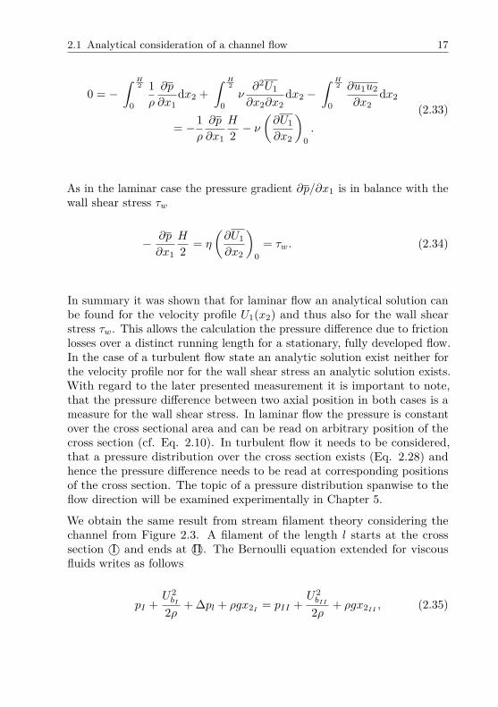
In summary it was shown that for laminar flow an analytical solution canbe found for the velocity profile 𝑈1(𝑥2) and thus also for the wall shearstress 𝜏𝑤. This allows the calculation the pressure difference due to frictionlosses over a distinct running length for a stationary, fully developed flow.In the case of a turbulent flow state an analytic solution exist neither forthe velocity profile nor for the wall shear stress an analytic solution exists.With regard to the later presented measurement it is important to note,that the pressure difference between two axial position in both cases is ameasure for the wall shear stress. In laminar flow the pressure is constantover the cross sectional area and can be read on arbitrary position of thecross section (cf. Eq. 2.10). In turbulent flow it needs to be considered,that a pressure distribution over the cross section exists (Eq. 2.28) andhence the pressure difference needs to be read at corresponding positionsof the cross section. The topic of a pressure distribution spanwise to theflow direction will be examined experimentally in Chapter 5.
We obtain the same result from stream filament theory considering thechannel from Figure 2.3. A filament of the length 𝑙 starts at the crosssection I○ and ends at II○. The Bernoulli equation extended for viscousfluids writes as follows
𝑝𝐼 +𝑈2
𝑏𝐼
2𝜌+ Δ𝑝𝑙 + 𝜌𝑔𝑥2𝐼
= 𝑝𝐼𝐼 +𝑈2
𝑏𝐼𝐼
2𝜌+ 𝜌𝑔𝑥2𝐼𝐼
, (2.35)

18 2 Fundamentals of air channel flows
where Δ𝑝𝑙 is the pressure loss. The continuity equation delivers 𝑈𝑏𝐼=
𝑈𝑏𝐼𝐼= 𝑈𝑏. The 𝑥2-position is the same for start and end of the flow
filament. We derive:
𝑝𝐼 − 𝑝𝐼𝐼 = Δ𝑝𝑙 (2.36)
The pressure loss due to wall friction is the only source to decrease thestatic pressure in flow direction. Thus the pressure drop is a measure forthe wall friction in the channel.
Figure 2.3: Consideration of pressure drop d𝑝d𝑥1
over a streamwise distance𝑙 based on flow filament theory
Law of the wall
The result for the turbulent channel does not offer as much physical insightas the complete laminar solution. However, some more information aboutthe near wall region of a turbulent flow can be obtained by examining thenear wall region via dimension analysis. Even in a turbulent flow the regionin direct vicinity to the wall is dominated by viscous forces in a very thinlayer. Fluctuations will be dampened due to the presence of the wall. Hence,the mechanism of momentum transport, similar to a laminar boundarylayer, is dominated by viscous forces. With growing distance from the wallthe inertial forces become dominate. To describe the functional relationsof wall bounded turbulent flows the following dimensionless quantities areagain derived from time-averaged mean values. The first quantity is thecharacteristic velocity for the near wall region named the friction velocity:

2.1 Analytical consideration of a channel flow 19
𝑢𝜏 =√
𝜏𝑤
𝜌. (2.37)
The viscous length scale is a measure for the smallest scales in the nearwall region:
𝛿𝜈 = 𝜈
√𝜌
𝜏𝑤= 𝜈
𝑢𝜏. (2.38)
These two characteristics quantities enable normalizing for velocity 𝑈+1
and the wall normal coordinate 𝑥2:
𝑈+1 = 𝑈1
𝑢𝜏, (2.39)
𝑥+2 = 𝑥2
𝛿𝜈. (2.40)
Turbulent wall-bounded flows can be described by a universal law. As Figure2.4 illustrates that the near wall flow is divided into to three layers. Closeto the wall, where viscous forces are dominating, the velocity distributionfollows a linear correlation 𝑢+ = 𝑥+
2 . The region of validity of this linearlaw is named the inner layer or viscous layer for 𝑥+
2 ≤ 5 from the wall.In a distance of 5 < 𝑥+
2 < 50 from the wall a region of transition to theouter layer exists: the buffer layer. Farther away from the wall the outeror logarithmic layer begins. The velocity distribution follows the universallaw (von Karman, 1930):
𝑢+ = 1𝜅
ln 𝑥+2 + 𝐵. (2.41)
This ”Law of the wall” wall has been developed by von Karman in adimensional analysis. It has two constants, which were originally determinedto 𝜅 = 0.41 and 𝐵 = 5.2. However, the accuracy of determination is stilldiscussed in the literature. Today’s state of scientific knowledge indicates𝜅 = 0.38 − 0.39 for the channel and boundary flow, while in a recentmeasurements for the Princeton super pipe 𝜅 = 0.42 was indicated (McKeonet al., 1999). Marusic et al. (2010) debate whether the two values are indeedconstants or slightly change with 𝑅𝑒.

20 2 Fundamentals of air channel flows
The linear and the logarithmic law deliver a description of the velocityprofile near a smooth wall in a turbulent flow. This important result isutilized in the course of the work to examine the adaption of the wall-lawto modifications of the surface condition.
100
101
102
103
0
5
10
15
20
25
x2
U+ 1
viscoussublayer
bufferlayer
logarithmiclayer
x <52
+ 5<x <502
+ x >502
+
u =1
x 2++
u = ln1
x +B2
+1k
+
Figure 2.4: Velocity profile of a turbulent flow in the region near to thewall.
2.2 Examination of the initial assumptionsfor ideal channel flow
At the beginning of this Chapter the hypothesis of an ideal channel flowhas been made to consider the analytic backgrounds. These assumptionsare simplifications, which cannot be transferred to the experiment withoutexamination. Some can be transferred to the experiment, while otherscan only be approximated. The following three assumptions require closerexamination to justify or restrict their validity in the experiments.
⇒ the two-dimensionality of the flow⇒ a fully developed flow state⇒ bounding walls are perfectly smooth

2.2 Examination of the initial assumptions for ideal channel flow 21
Two of these demands on the channel flow turn out to be challenging forexperimental investigations: The accomplishment of a full developmentas well as the two-dimensionality of the flow. While the full developmentcan be achieved by an adequate length of the channel, two-dimensionalityis limited to theoretical investigations. In theory it is possible to simplyassume infinite plates, which is represented by periodic boundary conditionsin numerical studies. But the physical realization of a channel of infinitedimension in spanwise direction is impossible. Hence for the experimentalinvestigations the question of a sufficient ratio between channel height 𝐻and width 𝑊 arises, which has been argued in numerous investigations inthe past (Durst et al. (1998), Monty (2005), Marusic et al. (2010), Nagibet al. (2013), Schultz & Flack (2013)). The following section will presentthe state-of-the-art, focusing on the aspect ratio 𝐴𝑆 = 𝑊/𝐻 and thedevelopment length 𝐿𝐸 for turbulent as well as laminar flow conditions.
Further we still have a lack of knowledge about the turbulent channel flowsince the analytic considerations do not provide a solution for the wallfriction 𝜏𝑤. Hence turbulent conditions require experimental and numericaldata to complete the picture. The following section will discuss step bystep these issues for laminar and turbulent flow conditions.
2.2.1 Concept of hydraulically smooth walls
One of the initial assumptions was the statement of perfectly smoothchannel walls. In an experiment the question arises, which quality of thesurface is convenient to approximate this criterion. This is a fundamentalquestion as far as improper reference surface would lead to overestimationof the skin friction reduction on the test surface.
To quantify the influence of the surface property Nikuradse (1933) per-formed measurements in a pipe flow. The surface roughness has beenvaried using adhesive layers with sand grains of different sizes. For thesmooth pipe Nikuradse found an excellent agreement with the law thatwas proposed by Blasius (1913). With 𝑅𝑒 based on the pipe diameter 𝐷the friction factor according to Darcy’s definition writes:
𝜆 = 4𝑐𝑓 = 0.316𝑅𝑒0.25 . (2.42)

22 2 Fundamentals of air channel flows
The comparison of the measurement with smooth and rough walls showed,that for a certain size of the sand grains, the friction in the pipe is increased,whereas it remains the same value as for the smooth pipe for smaller sandgrain. Thus the concept of hydraulically smooth surface was formulated,where, if the sand grain size is expressed in terms of dimensionless units,Nikuradse’s experiments indicated the flow to be unchanged by sand grainroughness height 𝑘 for 𝑘+ = 𝑘/𝛿𝜈 < 3.5. Over the years doubts towards thisconcept were growing for several reasons. The question arose whether ran-dom or distinct orientation of the surface morphology affects the influenceon the flow. Also the nature of sand grain of roughness may not be the onlyparameter to characterize the surface. For example the structure of sandgrain surface is to some degree affected by the binding material. Furthermissunderstanding arose due to Schlichting’s interpretation (Schlichting,1959) of Nikuradse’s data, who stated the flow to be unaffected up to𝑘+ = 5. Additionally, the conclusion of Nikuradse was influenced by themeasurement accuracy available at that time. In 2011 Gruneberger inves-tigated roughness elements in form of small fins orientated spanwise tothe flow direction (Gruneberger & Hage, 2011). He was able to accuratelymeasure dimensions slightly below ℎ+ = ℎ/𝛿𝜈 = 1 and influence on the flowwas still found. The type of roughness in this experiments is untypical forindustrially appearing imperfections, but a general limitation in the rangeof 𝑘+ = 3.5 could be disproved. From these experiments the conclusioncan been drawn, that the regime of hydraulically smoothness is foundfor ℎ+ < 1 - if such a regime exists at all. Bradshaw (2000) questionsthe existence of the hydraulically smooth regime in a passionate review.He concludes that there might be a boundary roughness below which theoutcome of engineering applications is no longer affected by the surfacemorphology. However, from a scientific point of view, such a boundaryroughness can probably not be found.
An estimate which has been shown to be appropriate for roughness typeoriginating from industrial fabrication is the characterization of roughnessbased on the roughness height 𝑘 to the pipe diameter 𝐷. Colebrook yieldeda formulation for the Darcy friction factor in dependence of 𝑘/𝐷 (Spurk &Aksel, 2006):
1√𝜆
= 1.74 − 2 log(
𝑘
0.5𝐷+ 18.7
𝑅𝑒√
𝜆
). (2.43)

2.2 Examination of the initial assumptions for ideal channel flow 23
The result is found in the diagram by Moody & Princeton (1944) andColebrook (1939) as shown in Figure 2.5 or the similar one by Nikuradse.The Moody-Colebrook diagram illustrates how roughness of a surface willenhance skin friction in a pipe flow. Within the turbulent regime roughnessis more critical with increasing 𝑅𝑒 since the influence of a roughness ofsame size increases with 𝑅𝑒 and the criterion of a ”hydraulically smoothsurface” tightens. For 𝑘+ > 70 the roughness significantly exceeds theregion of the buffer layer. Then the friction factor stays constant withincreasing 𝑅𝑒 (Spurk & Aksel, 2006), which defines a fully rough surface.
If we consider roughness in the layer to the law of the wall, roughness ofsize 𝑘 will modify the velocity profile:
𝑢+ = 1𝜅
ln 𝑥+2
𝑘+ + 𝐵 = 1𝜅
ln 𝑥+2 − 1
𝜅ln 𝑘+ + 𝐵. (2.44)
The additional term 1𝜅 ln 𝑘+ is a constant and the equation can be rewrit-
ten:
𝑢+ = 1𝜅
ln 𝑥+2 − Δ𝐵 + 𝐵. (2.45)
We obtain a reduction of the 𝐵 modification corresponding to a shifttowards the wall. Compared to the law of the wall for a hydraulicallysmooth surface the thickness of the viscous sublayer is reduced. For thefully rough surface the constant could be experimentally determined to𝐵 = 8.5:
𝑢+ = 1𝜅
ln 𝑥2
𝑘+ 8.5. (2.46)
In laminar flows roughness is of concern as it disturbs the flow triggeringthe transition process to turbulent flow. Since the flow velocities and the 𝑅𝑒will be very small in the present experiments, the surface is considered tobe smooth enough to keep laminar flow unaffected as long as the referencesurface will comply to the stricter turbulent criteria. For the presentinvestigation we will employ Gruneberger’s finding (Gruneberger & Hage,2011). Fulfilling the criterion ℎ+ < 0.5 for highest 𝑅𝑒𝑏 of the experimentalstudy, the influence of roughness is assumed to be so small, that it doesnot noticeably influence the skin friction. Therefore the requirements on a“hydraulically smooth” surface can be fulfilled easily in the experimentalinvestigation.
24 2 Fundamentals of air channel flows
1000 10000 100000 1000000 10
0,008
0,009
0,01
0,02
0,03
0,04
0,05
0,06
0,07
0,08
0,09
0,1
turbulentlamina
turbulent glatt
105
104
2104
410461048104
103
2103
4103
6103
8103
102
15102
2102
3102
4102
k/D = 5102
0.015
lam
bda
Re
l
3x10
6x10
1.5x10
108x10
k/D=5x10
4x10
2x10
10
6x108x10
4x10
2x10
10
10
laminar
4x10
2x10
5x10
turbulent
turbulent rough
turbulent smooth
7 108
2
2
2
2
2
2
3
3
3
3
3
4
4
4
4
4
5
5
roughness
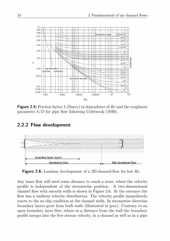
Figure 2.5: Friction factor 𝜆 (Darcy) in dependence of 𝑅𝑒 and the roughnessparameter 𝑘/𝐷 for pipe flow following Colebrook (1939).
2.2.2 Flow development
Figure 2.6: Laminar development of a 2D-channel-flow for low 𝑅𝑒.
Any inner flow will need some distance to reach a state, where the velocityprofile is independent of the streamwise position. A two-dimensionalchannel flow with smooth walls is shown in Figure 2.6. At the entrance theflow has a uniform velocity distribution. The velocity profile immediatelyreacts to the no slip condition at the channel walls. In streamwise directionboundary layers grow from both walls (illustrated in grey). Contrary to anopen boundary layer flow, where in a distance from the wall the boundaryprofile merges into the free stream velocity, in a channel as well as in a pipe

2.2 Examination of the initial assumptions for ideal channel flow 25
with increasing running length the growing boundaries layers meet at thecenterline. A distinction between boundary layer and undistorted flow, as itis the case in a zero gradient boundary layer, is not possible. The completecross-section is affected by the presence of the walls. In a fully developedstate inertial forces do not play a role, since the flow is not acceleratedor decelerated (Herwig, 2008). In developed flow the pressure gradientbalances the friction forces (compare Eq. (2.17) and Eq. (2.1.2)).
We will first consider a flow which develops from the channel entrancewithout any disturbances. This will be denoted as a “natural” developmentwhich is illustrated in Figure 2.6. At low Reynolds numbers the flowdevelops laminar. Starting from a constant velocity distribution over thecross section at the entrance, the flow forms a parabolic profile at thefully developed state as shown in the analytic consideration in 2.1.1. InSchlichting (1934) the flow development in a laminar channel is examinedtheoretically. The boundary layer region is treated by the approximationof boundary layer growth on a flat plate according to Blasius for bothwalls. As the boundary layers have grown together the calculation followsan asymptotic development to the parabolic profile. The result is a fastgrowth of the required development length 𝐿𝐸 with increasing 𝑅𝑒 forlaminar flow. Schlichting‘s result was confirmed to be quite appropriatein several experimental studies, where 𝐿𝐸/𝐻 was found in a range of0.055 − 0.68𝑅𝑒 (an overview is given in Durst et al. (2005)). The study byDurst et al. (2005) found slightly longer development length and suggestedthe empirical relation:
𝐿𝐸
𝐻= (0.6311.6 + (0.0442𝑅𝑒𝑏)1.6)1/1.6 (2.47)
which is illustrated in Figure 2.7.
With increasing Reynolds number inertial forces in the flow become domi-nant and the flow will become turbulent. At moderate 𝑅𝑒 the flow doesnot turn turbulent directly at the channel entrance as illustrated in Figure2.8. It will take a certain distance until disturbances have grown largeenough to initiate a transition to turbulent flow. The increase in lateralmomentum transfer enhances the flow development. So the developmentlength will be remarkably shortened compared to the laminar case. Thelaminar region at the entrance decreases with growing 𝑅𝑒𝑏.
The laminar to turbulent transition process can be accelerated, if distur-bances are induced through roughness of the surface or vibrations. Reynolds

26 2 Fundamentals of air channel flows
0 1000 2000 3000 4000 5000 6000 70000
50
100
150
200
250
300
350
Reb
LE/D
LE/H Durst et alLE/H Schlichting
Figure 2.7: Development length of a laminar channel flow according to thetheoretical consideration by Schlichting (1934) and the correlation derivedfrom experimental data by Durst et al. (2005).
Figure 2.8: Natural development of a 2D-channel-flow.
Investigations under turbulent flow conditions are usually artificially dis-turbed to shorten the development length and to generate a turbulent
(1883) observed the transition to occur between 𝑅𝑒 = 2000 and 13000 ina pipe, depending on the smoothness of the entry conditions. Usually𝑅𝑒𝑐𝑟𝑖𝑡 = 2300 is recommended for the onset of transition for a pipe anda flat channel. The critical Reynolds number 𝑅𝑒𝑐𝑟𝑖𝑡 is not a fixed value,but a general value below that laminar flow will persist in engineeringapplications. A flow that can develop without any disturbance persistslaminar up to significantly higher 𝑅𝑒𝑐𝑟𝑖𝑡. In this unstable state the flowpromptly turns turbulent, if a for instance disturbed by an agitation.

2.2 Examination of the initial assumptions for ideal channel flow 27
development at low Reynolds numbers. The development length of such atripped flow is controversially discussed, since the type and the size of thetripping device as well as the definition of a fully developed turbulent flowdiffer between the experimental studies. From an asymptotic approach inHerwig & Voigt (1995) a development length of 𝐿𝐸 = 25𝐻 is indicated tobe sufficient in a channel. This result is in accordance with experimentsfrom Byrne et al. (1970), while Durst recommends 60𝐻 (Durst et al., 1998).For a turbulent flow commonly the development length is recommended tobe independent of the Reynolds number (𝐿𝐸 = 𝑓(𝑅𝑒)).
The effectiveness of such tripping devices is limited by the Reynolds numberrange, beyond which the flow is totally dominated by viscosity. At verylow 𝑅𝑒 Nishioka & Masahito (1984) found even large distortions to bepromptly dampened and the flow to return to the laminar state. Theminimum Reynolds number beyond that disturbances can sustain over along distance in a channel was obtained about 𝑅𝑒 = 1400. This resultis confirmed very accurately by further experimental studies (Davies &White (1928), Carlson et al. (1982)) and also by the analysis of secondaryinstabilities by Orszag & Patera (1983). The lowest 𝑅𝑒 to achieve a fullyturbulent developed flow state is recommended by Durst et al. (1998) witha centerline Reynolds number of 𝑅𝑒𝑐 ≈ 3000, corresponding to 𝑅𝑒𝑏 ≈ 3500,which is in agreement with Nikuradse (1932). Nishioka & Masahito (1984)achieved fully turbulent conditions with a strong tripping for 𝑅𝑒𝑏 = 2400in a very long channel (𝐿 = 400𝐻).
One important aspect to allow to transfer measurement results from achannel flow for general application in turbulent flows, is the question whichReynolds number is required to achieve a flow state, where the gradient atthe wall will follow the log-law distribution. Nishioka & Masahito (1984)found the flow to partly follow the universal law for 𝑅𝑒𝑏 > 3000. Durst et al.(1998) found a universal behavior in the near all region (linear law) evenfor small turbulent 𝑅𝑒, but for 𝑅𝑒𝑏 ≤ 3000 their data show considerabledeviation for the region of the logarithmic law.
2.2.3 Approximation of two-dimensionality
As introduced at the beginning of this chapter, ideal two-dimensionalchannel flow is useful for the theoretical methods. If we speak abouta channel flow in the experimental context, an approximation with thegeometry of a flat duct is meant. A flat duct with the width 𝑊 and the

28 2 Fundamentals of air channel flows
height 𝐻 is characterized by the aspect ratio 𝐴𝑆 = 𝑊/𝐻. The fundamentaldifference of a turbulent flow in a flat duct to the flow between infiniteplates is illustrated in Figure 2.9. In a square duct secondary motions formwhich transport momentum to the corners. The result is a nearly constantdistribution of the wall shear stress in turbulent flows (Spurk & Aksel,2006). On the one hand these corner vortices balance the shear stress whichis favorable in context of a two-dimensional skin friction distribution inspanwise direction. On the other hand these secondary motions significantlyalter the flow field in the corners. For the flat duct the region influenced bythe secondary motions is limited to region of the sidewalls. Furthermore,additional friction is generated at the side walls compared to the flowbetween infinite plates.
The question arises on the aspect ratios needed to neglect the influence ofthe flow in vicinity to the sidewalls. In the literature differing estimatesare given depending on the definition of what can be accepted as still two-dimensional. While Dean found 𝐴𝑆 ≥ 7 satisfactory, Schultz & Flack (2013)use 𝐴𝑆 = 8, Marusic et al. (2010) states 𝐴𝑆 ≫ 10, Nagib recommends𝐴𝑆 ≥ 24 (Nagib et al., 2013) and (Durst et al., 1998) as well as Monty(2005) find 𝐴𝑆 = 12 adequate. The question of a sufficient approximationof a two-dimensional channel flow is closely connected to the question ofa sufficient development length. Experimental data of high aspect ratiotogether with large channel length are rare.
The contribution of numerical simulation to the topic on high aspect ratioducts is insufficient. The DNS simulation exhibiting the highest aspectratio 𝐴𝑆 = 7 known to the present author is the recent studies by Vinuesa(Vinuesa, 2013; Vinuesa et al., 2014). From the presented visualization ofcrossflow streamlines and magnitude it can be deduced, that an aspect ratioof seven is definitely too low for the small 𝑅𝑒𝑏 ≈ 2800. As will be shown inChapter 5 a real channel flow does not fulfill the criteria of a fully turbulentflow at such low 𝑅𝑒𝑏. With increasing Reynolds number the momentumexchange is also increasing and the flow field is rather approximating atwo-dimensional state.
For practical reason a ratio of 𝑊/𝐻 = 12 is chosen, which seems to beuseful in the present case. To get a profound information about the degreeof deviation from a two-dimensional state, the spanwise distribution of theskin-friction has been measured and is discussed in Chapter 5.

2.2 Examination of the initial assumptions for ideal channel flow 29
Figure 2.9: Schematic illustration of secondary motions in a square (left)and a rectangular duct (right) according to (Hoagland, 1960).
Influence of non-ideal 2D-flow on the skin friction coefficient
A fundamental study of experimental channel flow is the one from Dean(1978), who collected a lot of data from different investigators. The availabledata had been generated in facilities of differing characteristics. Finally27 sources dating from 1928 to 1976 were taken into account. Partly dataneeded to be recalculated to illustrate all data in one diagram showingfriction coefficient 𝑐𝑓 over 𝑅𝑒𝑏. Based on this data collection Dean developedhis famous fit for the friction factor in an experimental channel flow:
𝑐𝑓 = 0.073 𝑅𝑒(−0.25) (2.48)
The data collected by Dean show large scatter. Besides varying measure-ment accuracies of the different sources, the data is influenced by thevariation in the aspect ratio, reaching from 𝐴𝑆 = 7 to 169. Additionallythere is another influence that affects some of the data in Dean’s database: the length for flow development. For example Laufer (1951) andSkinner (1951) used a short channel with a length of 55𝐻 and let the flowdevelop only 20𝐻, which seems not appropriate, if we recall the valuesgiven by Herwig & Voigt (1995) and Durst et al. (1998). Yet, most sourcesused channels exhibiting 100 < 𝐿 < 300𝐻, for instance (Huebscher, 1947),some even 𝐿 > 300 for example (Hartnett et al., 1962). Dean himself wasaware of these facts and states both. Marusic et al. (2010) remark that thedevelopment length is one of the critical criteria leading to disagreementin available data and that there is still no common agreement concerningthe sufficient value. Nontheless, Dean‘s correlation represents a widelyaccepted approach which agrees very well with wide range of experimentalstudies.

30 2 Fundamentals of air channel flows
Figure 2.10: Friction coefficient 𝑐𝑓 : Correlations from experimental data(Dean, 1978; Johnston, 1973; Zanoun et al., 2009) in comparison to DNSresults by Hoyas & Jimenez (2008); Iwamoto et al. (2002); Moser et al.(1999).
Recently a refinement of Dean’s correlation was intended by Zanoun et al.(2009). Zanoun’s fit (Eq. 2.49) needs to be discussed here since it isbased on measurement data from a 𝐴𝑆 = 12 test section similar to presentchannel.
𝑐𝑓𝑍= 0.0743 𝑅𝑒(−0.25) (2.49)
Indeed the new correlation showed better agreement to the data of Zanounet al. (2009) as well as to the data of Monty (2005) than Dean’s law. Thecited sources are mainly interested in the investigation of universal flowquantities regarding high-𝑅𝑒 flow. Thus the developed empirical formulafor the friction coefficient focuses on 𝑅𝑒𝑏 ≫ 20.000, while the present workwill concentrate on comparably low-𝑅𝑒 flows which allows a comparisonto numerical simulations. For the range 𝑅𝑒𝑏 < 80000 still Dean yields thebetter fit to the mentioned experimental data. Yet, it should be realized,that experimental facilities can never provide a perfect two-dimensional flow.Evidence for the magnitude of the deviation to an ideal two-dimensional

2.2 Examination of the initial assumptions for ideal channel flow 31
flow can be obtained by considering DNS data. Kim et al. (1987) resultsshow 3% lower 𝑐𝑓 -values in comparison to Dean’s correlation in the low-𝑅𝑒range. The deviation becomes smaller with increasing 𝑅𝑒. Figure 2.10compares the correlation from Dean, the older one from Johnston (1973)𝑐𝑓𝐽
= 0.0706 𝑅𝑒(−0.25) and the recent fit by Zanoun. The data pointsindicate the results originating from DNS. Note that all correlations usethe same functional relation 𝑐𝑓 = 𝑘 𝑅𝑒(−0.25) and only modify the constant𝑘. It can be conjectured that it is impossible to match the experimentaldata for the whole range of 𝑅𝑒 on that basis. The resulting value of theconstant is a function of the Reynolds number.
Influence of secondary motions on flow development
As shown in Figure 2.9 secondary motions influence the turbulent flow in aflat duct. Studying laminar flow through a flat duct Arbeiter (2009) showeda successive transport of fluid from the side wall region to the center of theduct. In personal communication Arbeiter mentioned that this mechanismwas still not finished over quite large run length (𝐿𝐸=80). This may explainthe slight difference in 𝐿𝐸 reported between Schlichting’s theoretical andexperimental studies (cf. Chapter 2.2.2). A special issue is the effect onlaminar-turbulent transition in the duct. In an ideal two-dimensional flowthe transition process is initiated by small disturbances that are developingwith the run length as it is the case in a pipe flow experiment. However,in a flat duct disturbances unavoidable appear in the form of the cornervortices, which are growing stronger with increasing 𝑅𝑒. Thus secondarymotions can induce transition starting from the ”inflectionally-unstablecorner boundary layers” (Dean, 1978), which is distinctively visualized inArbeiter et al. (2008). Arbeiter reports a drastic increase of turbulencewithin the streak regions at the side walls.
Since no particular information for the development of the vortex dominatedregion at the sidewalls for a flat duct was found in the literature, an estimateof the influence of the sidewalls on the transition process is drawn fromthe flat plate experiments by King & Breuer (2001, 2002). Their windtunnel exhibits a conventional layout of 𝐻 = 2ft and 𝑊 = 3ft with a flatplate located horizontally in the center (Fig. 2.11). King & Breuer (2001)illustrate a contamination with an angle 12∘ on the plate originating fromthe side walls. If we consider the cross section being divided by the flatplate, the obtained sidewall contamination can be transferred to each of

32 2 Fundamentals of air channel flows
the two flat ducts with an 𝐴𝑆 = 3. The angle of 12∘ is in agreementwith the photograph shown in Arbeiter (2009) from a channel exhibiting𝐴𝑆 = 10. It can be deduced that for moderate aspect ratios the sidewallcontamination is influencing the transition process.
As a consequence a hydraulically smooth duct will have a certain 𝑅𝑒where transition is occurring (Dean, 1978). This situation is fundamentallydifferent to the pipe, where the condition of the inlet is the main parameterinfluencing the transition process. If not disturbed, a pipe flow can remainlaminar up the very large 𝑅𝑒.
W/H=3/2
flat plate12°
sidewall contamination
W
H
Figure 2.11: Schematic sketch of side wall effect in the wind tunnel ex-periment of King & Breuer (2001), including cross sectional and top view.
2.3 Properties of air
In terms of aerodynamic considerations certain characteristics of the gasmixture air − mainly consisting of nitrogen and oxygen − are from relevance.For the present study the density 𝜌 and the dynamic viscosity 𝜂 are ofmajor interest.
In the first instance we regard the properties of a fluid employing the idealgas law (Eq. 2.50). With the static pressure 𝑝 and ambient temperature𝑇 as well as the specific gas constant 𝑅𝑠, the density can be determined.Using the standard conditions from table 2.1 defined in White (1974),corresponding to German engineer standard DIN2533 (Czichos & Hennecke,2004) we yield a density of 𝜌 =1.225kg/m3. The right graph in Figure 2.12depicts the behavior of the air density at norm temperature in range of themeteorological fluctuation of the atmospheric pressure, while the left oneshows the equivalent for temperature variation at a standard pressure of1013.25hPa

2.3 Properties of air 33
14 16 18 20 22 241.18
1.19
1.2
1.21
1.22
1.23
T [◦C]
ρ[kg/m
3]
960 980 1000 1020 1040
1.16
1.18
1.2
1.22
1.24
1.26
p[hPa]
ρ[kg/m
3]
Figure 2.12: Air density within the temperature range of the laboratory(left) and in dependence of typical variations of the atmospheric pressure(right).
𝑝 𝑉 = 𝑛 𝑅 𝑇 = 𝑅𝑠 𝑇 ⇔ 𝜌 = 𝑝
𝑅𝑠𝑇(2.50)
Additionally, the density is affected by the humidity in the air (Fig. 2.13).The air humidity can be taken into account by determining the gas constantof the air-vapor mixture 𝑅𝑓 . Following the empirical formula (2.52) fromMagnus, the saturation vapour pressure 𝑝𝑑,𝑠 is calculated. The air humidityℎ is inserted in the common form as the percentage of vapor which theair can maximal contain. Further the specific gas constants for air 𝑅𝑙 andvapor 𝑅𝑑 are required
𝜌 = 𝑝
𝑅𝑓 𝑇with 𝑅𝑓 = 𝑅𝑙
1 −(
ℎ𝑝𝑑,𝑠
𝑝
) (1 − 𝑅𝑙
𝑅𝑑
) (2.51)
𝑝𝑑,𝑠 = 𝑝𝑑,𝑠,0 exp(
17.5043 · (𝑇 − 273.15)𝑇 − 31.95∘𝐾
). (2.52)
Also the dynamic viscosity 𝜂 is a function of 𝑝 and 𝑇 :
𝜂 = 𝑓(𝑇, 𝑝𝑏𝑎𝑟). (2.53)
As depicted in the diagram 2.14(a), 𝜂 is weakly dependent on the barometricpressure. For instance a pressure increase from standard pressure to 5bar

34 2 Fundamentals of air channel flows
0 20 40 601.16
1.17
1.18
1.19
1.2
1.21
1.22
1.23
h[%]
ρ[kg/m
3]
t = 15◦Ct = 20◦Ct = 25◦C
Figure 2.13: Dependence of air density on the humidity for different tem-peratures.
air at normal state (DIN ISO 2533)standard pressure 𝑝𝑛 101325Paspecific standard temperatur (DIN 1343) 𝑇𝑛 228.15K=15∘ Cdensity of dry air 𝜌𝑛 1.225 kg/m3
specific gas constant of dry air 𝑅𝑙 287.05287J/(kgK )dynamic viscosity 𝜂𝑛 17.894𝜇Pa·sspecific gas constant of vapor (VDI 2002) 𝑅𝑑 461.526J/(kgK )Sutherland constant (White 1974) 𝑆 110.556
Table 2.1: Standard conditions of air according to DIN ISO 2533, Suther-land constant 𝑆 and specific gas constant of water steam 𝑅𝑠

2.3 Properties of air 35
100
101
102
1.5
2
2.5
3x 10
−5
p[bar]
η[Pas]
(a)
14 16 18 20 22 241.78
1.79
1.8
1.81
1.82
1.83
1.84
1.85x 10
−5
t[◦C]
η[Pas]
(b)
Figure 2.14: Air viscosity as a function of the pressure according to VDI(2002) (a) and in dependence of the temperature in the laboratory (b).
alters the viscosity by only 0.2%. Taking into account the small fluctuationsof the atmospheric pressure of Δ𝑝𝑏𝑎𝑟,𝑚𝑎𝑥 = ±40hpa the effect on 𝜂 neglected.In consequence the viscosity solely depends on the temperature, so thevariation can be determined according to Sutherland‘s formula (Eq. 2.54from White (1974)) as shown in Figure 2.14(b).
𝜂 (𝑇 ) = 𝜂0𝑇0 + 𝑆
𝑇 + 𝑆
(𝑇
𝑇0
) 32
(2.54)
The Sutherland constant 𝑆 and the reference temperature 𝑇0 also corre-spond to the definition from White (1974) in table 2.1.
Depending on the literature source, differing information at various referencepoints are specified for standard parameters of air. If Sutherland‘s formulais used to convert to a concerted reference point, differences in the calculatedair viscosity result. Values given in White (1974) differ from VDI (2002)about 0.5%. If we consider that the viscosity affects the Reynolds numberproportional to 1/𝜂, this deviation is of the order of the errors in the flowrate measurement presented in Chapter 4. In the present study a potentialsystematic deviation would not affect the result of the percentage reductionof skin friction, but it shows that the reference source needs to be chosencarefully. The author cannot say which source is the most exact. Thereference values of White (1974) are chosen to stay conform with otheraerodynamic research.


3 Experimental setup
The following section presents the experimental setup, that has beendesigned and built within the project. The discussion will be divided inthree main parts. The first part provides a detailed description of thewind tunnel, while the second part considers the test section. Part threeintroduces the measurement equipment and examines the interaction of thecomplete system focusing on the capabilities of the set-up in combinationwith the channel test section. It is followed by a detailed estimation of themeasurement uncertainty in the subsequent chapter.
3.1 Wind tunnel
In the context of the present project special requirements on the windtunnel are addressed, which are found in a configuration denoted “blowertunnel”, where the fan is installed upstream the test section. The blowerconfiguration is advantageous with respect to effective wind tunnel controland uniformity of the flow rate (Pope & Harper, 1966). In the particularcase of the present project, the type of a wind tunnel in its specificationas a modification of a ventilator test rig according to DIN 24163 (1985) isrecommend due to requirements in highly accurate flow rate measurementand large pressure built-up. Facilities of this type are widely-used and oftenmodified to extend the initial intended field of operation. For instancefacilities of this type run at institutes FSM at KIT in Karlsruhe and LSTMat Friedrich-Alexander-Universitat in Erlangen (Spudat, 1981). In contrastto the present set-up, these facilities were designed and built for comparablyhigh flow rates. Both serve as basic instrument for scientific research formany decades. LSTM in Erlangen provided the opportunity to inspecttheir facility, which is intermittently used in very similar experiments witha comparable test section configuration as the one designed for the presentstudy.
38 3 Experimental setup
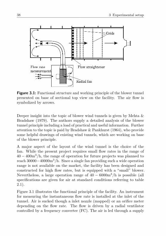
Figure 3.1: Functional structure and working principle of the blower tunnelpresented on base of sectional top view on the facility. The air flow issymbolized by arrows.
Deeper insight into the topic of blower wind tunnels is given by Mehta &Bradshaw (1979). The authors supply a detailed analysis of the blowertunnel principle including a load of practical and useful information. Furtherattention to the topic is paid by Bradshaw & Pankhurst (1964), who providesome helpful drawings of existing wind tunnels, which are working on baseof the blower principle.
A major aspect of the layout of the wind tunnel is the choice of thefan. While the present project requires small flow rates in the range of40 − 400m3/h, the range of operation for future projects was planned toreach 30000−40000m3/h. Since a single fan providing such a wide operationrange is not available on the market, the facility has been designed andconstructed for high flow rates, but is equipped with a “small” blower.Nevertheless, a large operation range of 40 − 6000m3/h is possible (allspecifications are given for air at standard conditions referring to table
Figure 3.1 illustrates the functional principle of the facility. An instrumentfor measuring the instantaneous flow rate is installed at the inlet of thetunnel. Air is sucked though a inlet nozzle (mapped) or an orifice meterdepending on the flow rate. The flow is driven by a radial ventilatorcontrolled by a frequency converter (FC). The air is led through a supply
2.1).
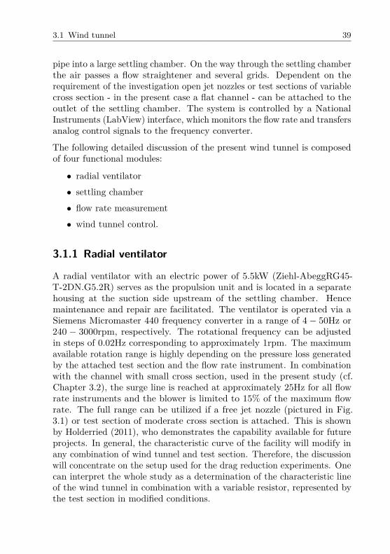
3.1 Wind tunnel 39
pipe into a large settling chamber. On the way through the settling chamberthe air passes a flow straightener and several grids. Dependent on therequirement of the investigation open jet nozzles or test sections of variablecross section - in the present case a flat channel - can be attached to theoutlet of the settling chamber. The system is controlled by a NationalInstruments (LabView) interface, which monitors the flow rate and transfersanalog control signals to the frequency converter.
The following detailed discussion of the present wind tunnel is composedof four functional modules:
∙ radial ventilator
∙ settling chamber
∙ flow rate measurement
∙ wind tunnel control.
3.1.1 Radial ventilator
A radial ventilator with an electric power of 5.5kW (Ziehl-AbeggRG45-T-2DN.G5.2R) serves as the propulsion unit and is located in a separatehousing at the suction side upstream of the settling chamber. Hencemaintenance and repair are facilitated. The ventilator is operated via aSiemens Micromaster 440 frequency converter in a range of 4 − 50Hz or240 − 3000rpm, respectively. The rotational frequency can be adjustedin steps of 0.02Hz corresponding to approximately 1rpm. The maximumavailable rotation range is highly depending on the pressure loss generatedby the attached test section and the flow rate instrument. In combinationwith the channel with small cross section, used in the present study (cf.Chapter 3.2), the surge line is reached at approximately 25Hz for all flowrate instruments and the blower is limited to 15% of the maximum flowrate. The full range can be utilized if a free jet nozzle (pictured in Fig.3.1) or test section of moderate cross section is attached. This is shownby Holderried (2011), who demonstrates the capability available for futureprojects. In general, the characteristic curve of the facility will modify inany combination of wind tunnel and test section. Therefore, the discussionwill concentrate on the setup used for the drag reduction experiments. Onecan interpret the whole study as a determination of the characteristic lineof the wind tunnel in combination with a variable resistor, represented bythe test section in modified conditions.

40 3 Experimental setup
3.1.2 Settling chamber
The settling chamber consists of 4mm thick cylindrical steel casing withribbing for reinforcement configured for a system pressure of Δ𝑝𝑚𝑎𝑥 =0.05bar. The length is 𝐿 = 4800mm and the inner diameter is constant(𝑑𝑖 = 1760mm). The inflow of the air is implemented via a supplyingpipe (𝐷𝑅 = 400𝑚𝑚), which directs the air to the headwall of the chamber(compare Figure 3.1). The arrangement to blow the air towards the endwall is adopted from the facility in Erlangen (Spudat, 1981). It may notseem intuitive to blow contrary to the main flow direction into the chamber.Alternatively, the length required to expand a free jet, which is blowingupstream in the chamber, to a homogeneous velocity distribution over thediameter of the settling chamber needs to be considered. If the installationof auxiliary components such as grids or perforated plates to shorten thislength would at least lead to less pressure losses in the settling chamberremains questionable.
In the downstream section of the settling chamber the diameter of the steelcasing expands to gain additional space for a cribbing with wooden rings(glued laminated beech 30mm, 𝑑𝑖 = 1760mm). The wooden rings carry 5grids (𝑑=2mm, blockage 56%, stainless steel) and fix the flow straightener(TUBUS honeycomb PC6.0 − 70 depth 100mm). By opening the end coveron the outlet side the rings can be removed or exchanged. This enables tovary the distance between the grids or to equip the rings with meshes ofdifferent width.
The functionality of the settling chamber needs to be considered for twodifferent ranges of the flow rates. For small flow rates (< 900m3/h) themean velocity in the chamber remains smaller than < 0.1m/s. Thus, thechamber is practically a settled plenum. If the operating range of thefacility is expanded to the maximum capabilities for flow rates of up to40.000m3/h, the grids become effective.
Again the arrangement of the ventilator outside the settling chamber hasimportant benefits. On its way through the settling chamber the flow doesnot pass the blower, but only the supplying pipe with a comparable smallblockage. Additionally the positioning of the drive unit is favorable todecouple the vibrations and to some extent the noise generated by theventilator. On the other hand the selected arrangement turns out to bedisadvantageous due to the larger distance the flow has to cover from theinlet to the outlet of the facility. The resulting pressure losses, in particularat the low flow rates of the actual operation range, are insignificant.

3.1 Wind tunnel 41
The selected arrangement has been chosen to generate a homogeneous andsymmetric velocity distribution at the outlet. Holderried (2011) verifiedthe homogeneous distribution of velocity and low turbulence level in a freejet configuration for various outlets diameters and flow rates.
The accessibility of the settling chamber for repair, maintenance or cleaningof the inside is of fundamental importance for the everyday work. Therefore,the facility offers two possibilities to enter the settling chamber on each side:The access through the window at the bow or a removal of the complete900mm-section at the inlet side. On the outlet side of the chamber one canenter through the standard flange with 𝑑𝑜𝑢𝑡 = 800mm or, as mentionedbefore, open the full diameter by unfastening the front cover. The commonuncomfortable and costly construction with a manway opening is avoided.
Figure 3.2: Illustration of the settling chamber including partly a sectionalview to depict the inner workings.

42 3 Experimental setup
3.1.3 Flow rate measurement
In general the working principle of the selected types of flow rate meters isbased on the measurement of the differential pressure between the staticpressure in the flow in a pipe and the total pressure at a stagnation point.The obtained differential pressure is proportional to the square of the fluidvelocity. The flow rate �� can be determined as follows (DIN24163-2):
�� = 𝑘 𝐴
√2Δ𝑝
𝜌. (3.1)
The constant 𝑘 is dependent in the expansion number 𝑒 and a typical flowcoefficient, which is a function of the Reynolds number and the characteristicgeometry depending on of flow meter type. 𝐴 is the cross section area ofthe instrument.
In the present study the wind tunnel can be equipped with two types ofdifferential pressure based flow rate instruments. Depending on the flowrate inlet nozzles or orifice meters are chosen for the flow rate determination.Both types of flow rate meters are used in combination with two SetraD239 sensors with different measuring ranges and an accuracy of 0.07% oftheir full scale (FS). Since the pressure difference at the flow meters forboth types of instruments to a large portion generates dissipative loss, itcan have a considerable influence on the operation range of the facility.In order not to limit the capabilities of the facility by generating highpressure loss in the flow measurement, a maximum differential pressure ofΔ𝑝𝑚𝑎𝑥 = 625Pa was selected. Due to the accuracy of the sensors, the lowerlimit of reading was restricted to an operation range of Δ𝑝 = 18 − 125Paand 123 − 625Pa.
Inlet nozzles
Inlet nozzles are widely used devices for flow metering complying withengineer standards DIN 24163 (1985) and DIN EN ISO 5167-2 (2003). Highaccuracy, small space requirement, simple manufacturing and comparablylow pressure losses at high flow rates characterize these instruments. Fromthe different types of inlet nozzles the construction following DIN24163-2“Viertelkreismessduse” was chosen (Figure 3.3). The version with four

3.1 Wind tunnel 43
1.5
D
D
0.5D >1.6D0.25D
r=0.2
5D
Figure 3.3: Cross sectional view of an inlet nozzle of the chosen type withquarter cycle inlet.
pressure taps of a diameter of 0.3mm placed equidistantly over the circum-ference was selected. Five nozzles of diameters of 50mm, 74mm, 112mm,168mm and 262mm have been built at the workshops of the institutesSLA and PTW in Darmstadt. In combination with the Setra sensors anoperation range of �� = 200 − 5300m3/h is covered.
The determination of the flow rate is based on a measurement of the staticpressure difference between a certain position in the nozzles and the ambientpressure 𝑝𝑏𝑎𝑟. As illustrated in Figure 3.3 the pressure tab is located at adistance of 0.5𝐷 from the inlet. At this position a minimum developmentof the flow can be assumed and the cross sectional velocity distributionis nearly constant. As far as a turbulent flow state is achieved the flowcoefficient 𝛼 is delivered by a calibration function according to DIN:
𝛼 = 1 − 0, 004
√106
𝑅𝑒𝐷with 𝑅𝑒𝐷 = 𝑈𝑏 𝐷
𝜈. (3.2)
To obtain turbulent flow at the tap position, 𝑅𝑒𝐷 ≥ 100000 is required.Thus for a certain nozzle diameter 𝐷 a lower limit of the operation rangeresults. In general a nozzle of smaller diameter enables a lower minimum

44 3 Experimental setup
flow rate. But smaller diameters result in larger velocities to reach theReynolds number requirement. In consequence a very small nozzle would bea pure generator of pressure loss due to increased friction. Therefore, DIN24163 (1985) formulates a practical limit of 𝐷𝑚𝑖𝑛 = 50mm correspondingto approximately �� = 200m3/h. Since the specification for the presentproject was to measure flow rates down to �� = 40m3/h, alternative flowrate instruments are required.
An extension of the operating range of inlet nozzles below the lower limitby calibration is discussed in Appendix A.1.
Orifice meter
Due to the limitation of the operation range of the inlet nozzles, an orificemeter run conform to DIN EN ISO 5167-2 (2003) has been installed for themeasurement of small flow rates. In an orifice meter the pressure differenceupstream and downstream in vicinity of a thin orifice plate is measured(Figure 3.4). The flow rate can be determined following equation 3.3:
�� = 𝐶√1 − 𝛽4
𝑒𝜋
4 𝑑2
√2Δ𝑝
𝜌(3.3)
with the diameter ratio of orifice diameter to pipe diameter 𝛽 = 𝑑/𝐷and the flow coefficient 𝐶 derived from empirical the formula by Reader-Harris/Gallagher (Reader-Harris & Sattary, 1996), which simplifies for thepresent orifice design to:
𝐶 = 0.5961 + 0.0261𝛽2 − 0.216𝛽8 + 0.000521(
106𝛽
𝑅𝑒𝐷
)0.7
+ (0.0188 + 0.0063𝐴) 𝛽3.5(
106𝛽
𝑅𝑒𝐷
)0.3
(3.4)
In contrast to the inlet nozzles, the orifice meter work based on a fullydeveloped turbulent state of the flow and the corresponding velocity profile.A running length of ≥ 30𝐷 to the position where the orifice can be installed

3.1 Wind tunnel 45
is required, which demonstrates the major advantage of inlet nozzles due toreduced requirement of space. The turbulent flow state is reliably generatedfor 𝑅𝑒𝐷 > 5000 − 6000, corresponding to approximately 5% of the velocityin a comparable inlet nozzle of same pipe diameter. At the same time thedifferential pressure at the disc is slightly higher than in the equivalentnozzle, which at low flow rates is beneficial with respect to the measurementaccuracy of the pressure sensors.
dD
32D
Figure 3.4: Cross sectional view of the orifice meter run with annularchamber type. The connection to the pipe is equipped with centeringflanges.
In the present study the orifice meter run consists of an aluminum pipewith a diameter 𝐷 = 100.2mm and two exchangeable disks of 𝑑𝐵 = 60mmand 𝑑𝐵 = 75mm. In combination with the available pressure sensorsan operation range of �� = 40 − 370m3/h is covered. The length of theseamless pipe is 4000mm, thereof 3200mm are used for the flow development.To ensure fully developed turbulent flow at smallest flow rates, a zig-zag tripping is installed in direct vicinity to the inlet. The measuringchamber (annular chamber type, Figure 3.4) is custom manufactured (IntraAutomation) fitting with an diameter accuracy of tenth of a millimeter tothe pipe diameter. The latter is equipped with special centering flangesto precisely align with the chamber. Thus the fabrication tolerances areeven significantly better than the specifications according to the norm. Anoverview of the operation range for both instrument types is given in tables3.1 and 3.2.

46 3 Experimental setup
Table 3.1: Operation range of inlet nozzles.nozzle diameter [mm] ��𝑚𝑖𝑛 [m3/h] ��𝑚𝑎𝑥 [m3/h]
50 190 22574 225 500112 470 1150168 700 2570262 1620 6250
Table 3.2: Operation range of orifice meters.orifice plate diameter [mm] ��𝑚𝑖𝑛 [m3/h] ��𝑚𝑎𝑥 [m3/h]
60 38 22575 68 370
3.1.4 Wind tunnel control
For controlling the flow rate the user can choose between two alternativesystems: a LabVIEW-based computer control and a manual analog control.The latter control mainly served for testing during the development of thefeed-back control. In both control modes the rotation speed is regulatedusing the internal control circuit of the frequency converter, which hasbeen custom-programmed for the facility. A personal computer calculatesthe actual flow quantities: flow rate and velocity in dependence of theconnected test section and the type of the flow meter. The computedvalues are displayed together with the measurement reading of the pressuredifference at the flow meter and ambient measurement quantities as wellas the computed values for the density 𝜌 and the kinematic viscosity 𝜈.
In the manual mode the rotation speed is adjusted with a potentiometerand the setting is indicated at the display of the frequency converter. Anydigital indicator of the computer controlled system can run simultaneouslyand the full functional range is preserved.
A detailed description of the control software can be found in the thesis ofHolderried (2011).

3.2 Test section 47
3.2 Test section
The main issue concerning the design of the test section is the choice ofits aspect ratio. Various recommendations can be found in literature, asmentioned in Chapter 2.2.2, thus an appropriate compromise was foundfor 𝐴𝑆 = 12. An aspect ratio of 𝐴𝑆 = 20 would have been desirable, butthe enormous difference between width and height, would have requireda modified layout of cross section geometry of the settling chamber. Thisseemed not to be reasonable with respect to the wide range of operationthe facility has been projected to run in future projects. The second designobjective learned from the literature is the required length to fully developthe flow, especially in the laminar flow case. In this respect the limitationarose from the available space in laboratory: A total length of maximum4500mm was feasible. A channel height of 25mm has been chosen to beable to realize a total channel length of 150𝐻.
950mm 1500mm 1500mm
Figure 3.5: Top view of the channel test section with nozzle.
350mm
300mm
25.2mm
15mm
Figure 3.6: Cross sectional view of the channel test section.
Although the channel could have been longer in terms of multiples of thechannel height, 𝐻 was not chosen smaller due to the fabrication tolerances.These considerably affect the measurement accuracy of the flow velocity inthe test section for a smaller channel height.
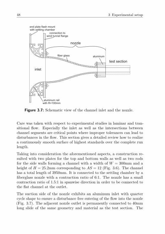
48 3 Experimental setup
nozzle
aluminum
inlet
test section
fiber glass
connection towind tunnel flange
end plate flash mountwith settling chamber
aluminum railwith R=100mm
Figure 3.7: Schematic view of the channel inlet and the nozzle.
Care was taken with respect to experimental studies in laminar and tran-sitional flow. Especially the inlet as well as the intersections betweenchannel segments are critical points where improper tolerances can lead todisturbances in the flow. This section gives a detailed review how to realizea continuously smooth surface of highest standards over the complete runlength.
Taking into consideration the aforementioned aspects, a construction re-sulted with two plates for the top and bottom walls as well as two rodsfor the side walls forming a channel with a width of 𝑊 = 300mm and aheight of 𝐻 = 25.2mm corresponding to 𝐴𝑆 = 12 (Fig. 3.6). The channelhas a total length of 3950mm. It is connected to the settling chamber by afiberglass nozzle with a contraction ratio of 6:1. The nozzle has a smallcontraction ratio of 1.5:1 in spanwise direction in order to be connected tothe flat channel at the outlet.
The suction side of the nozzle exhibits an aluminum inlet with quartercycle shape to ensure a disturbance free entering of the flow into the nozzle(Fig. 3.7). The adjacent nozzle outlet is permanently connected to 40mmlong slide of the same geometry and material as the test section. The

3.2 Test section 49
connection to the test section is therefore quite perfect. The glass fiberpart fitted accurately to the air inlet, to the aluminum connector on thetest section side with a step of less than 5/100mm. Both intersectionshave been carefully filled and sanded with an excellent final result. Thelong-term smoothness of the junction between the the materials aluminumand glass fiber may be be problematic if large temperature differences areencountered. For the present investigation, however, no decrease of qualitywas been observed.
The test section itself is divided into two parts with respect to the maximumavailable length of the aluminum for the side walls of 3020mm. The firstpart has a length of 950mm, the second part of 3000mm. To ensure that allsidewalls are identical in height, all parts were parallely cut from the sameplate in direction of grain. The side parts are straight in line without anydeflection. To connect the two segments of the test section without any steptwo guide plates are mounted parallel planar to the side walls as shown inFigure 3.9. This construction turned out to be advantageous: Now, there isa perfect intersection. For changing the cover plates in the long downstreamsection, the nozzle and the first test section part can remain unchanged.As a result, handling of the test section in case of exchanging the top andbottom plates is relatively easy. To enable replacement, these plates arescrewed to the side walls. The cover plates are divided into sections of950mm, 1500mm and 1500mm as shown in Figure 3.5. To guarantee asmooth surface, the top and bottom walls are made from cast aluminumwith a precision milled surface, exhibiting a roughness of 𝑅𝑎 = 0.4𝜇m,while the sidewalls were sanded to equivalent quality (sand grain 1000).
Along the side walls 21 pairs of pressure taps are located which allows aconvenient exchange of the top and bottom plates without pressure taps onthe test plates. This avoids the difficulty of manufacturing pressure tabs ina structured surface of test plates and guarantees the exact same positionand quality of the taps. The first tap is 100mm from the channel entranceand the streamwise distance between the taps is equidistant each 200mm.At the intersections between the cover plates the distance between theneighboring taps is 100mm. This allows to observe eventual misalignment,which would result in a change of the local pressure gradient. It will beshown in Chapter 5 that there is no evidence for a flow disturbance at theintersections. The tabs are positioned at the same streamwise positionson both side walls. Counterpart taps are short cut via a pressure line andyield one averaged reading.

50 3 Experimental setup
Figure 3.8: Schematic illustration of the construction of the pressure taps.
top andbottom plates
side walls
guide plate
Figure 3.9: Schematic illustration of the connection between segments ofthe channel section.
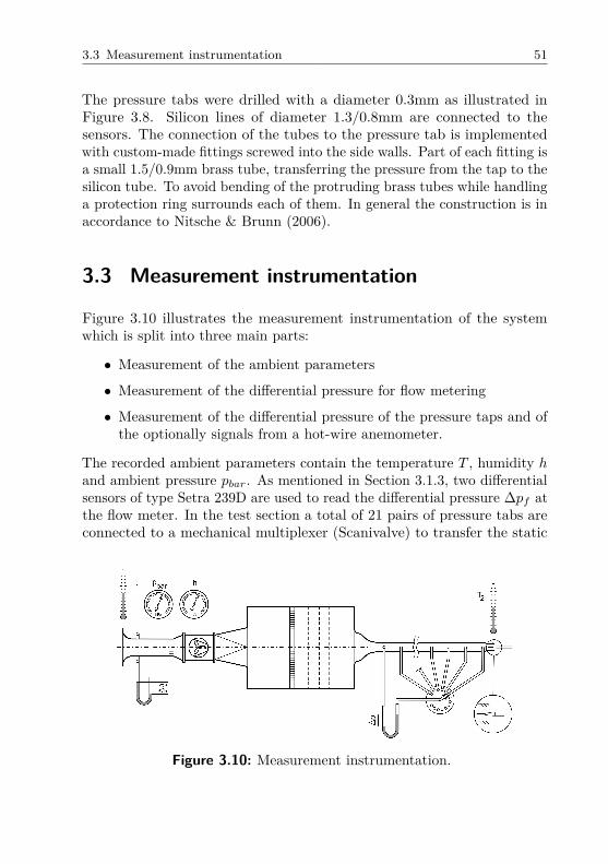
3.3 Measurement instrumentation 51
The pressure tabs were drilled with a diameter 0.3mm as illustrated inFigure 3.8. Silicon lines of diameter 1.3/0.8mm are connected to thesensors. The connection of the tubes to the pressure tab is implementedwith custom-made fittings screwed into the side walls. Part of each fitting isa small 1.5/0.9mm brass tube, transferring the pressure from the tap to thesilicon tube. To avoid bending of the protruding brass tubes while handlinga protection ring surrounds each of them. In general the construction is inaccordance to Nitsche & Brunn (2006).
3.3 Measurement instrumentation
Figure 3.10 illustrates the measurement instrumentation of the systemwhich is split into three main parts:
∙ Measurement of the ambient parameters
∙ Measurement of the differential pressure for flow metering
∙ Measurement of the differential pressure of the pressure taps and ofthe optionally signals from a hot-wire anemometer.
The recorded ambient parameters contain the temperature 𝑇 , humidity ℎand ambient pressure 𝑝𝑏𝑎𝑟. As mentioned in Section 3.1.3, two differentialsensors of type Setra 239D are used to read the differential pressure Δ𝑝𝑓 atthe flow meter. In the test section a total of 21 pairs of pressure tabs areconnected to a mechanical multiplexer (Scanivalve) to transfer the static
Figure 3.10: Measurement instrumentation.

52 3 Experimental setup
pressure Δ𝑝𝑙 to pressure transducers (MKS Baratron 698A). Optionally ahot-wire can be installed at the tunnel outlet for measuring the turbulencelevel in the channel.
The interplay of the system is characterized by the collection of measurementdata, the communication between components for signal processing andthe wind tunnel control as well as the synchronized storage of the data.An overview is presented in Figure 3.11.
The data is acquired by two computers − one for the wind tunnel controland one for the data acquisition at the test section. While the task of thetunnel computer is to deliver the flow rate and the air properties, the testsection computer collects the readings of the pressure drop measurementand the hot-wire anemometer. In detail the wind tunnel computer sendsthe input commands for the rotation speed of the ventilator to the FC. Thecommunication operates via AD/DA-converter (National Instruments (NI)USB-6211) to activate the internal controller of the FC. The same deviceis utilized to digitize the readings of three PT100 resistance thermometersreporting the temperature at the inlet of the orifice meter, at the inlet ofthe nozzle and at the outlet of the tunnel. Additionally the differentialpressure Δ𝑝𝑓 from the Setra Sensors of the flow meter is recorded. Twohumidity sensors (Sensirion SHT2) are directly connected to the PC viaUSB and the ambient pressure 𝑝𝑏𝑎𝑟 sources from manual input (source:meteorological station of Hessisches Landesamt fur Umwelt und Geologie(HLUG)). From this data collection the air quantities 𝜌 and 𝜂 are computed,which are needed for the accurate calculation of the flow quantities 𝑅𝑒𝑏,�� and 𝑈𝑏. Via network communication these quantities are send to themeasurement computer.
The measurement computer simultaneously acquires data, receives a contin-uous data flow from the wind tunnel control and synchronously saves thesedata on the hard disk. This computer is located at the test section andcontrols the Scanivalve multiplexer via an AD/DA-converter (NI-6009) toswitch between the positions of the pressure taps connected of the pressuretransducers. In the opposite direction position report of the Scanivalveis received. Two parallely driven Scanivalve multiplexers are used, eachconnected to a highly accurate capacitive pressure sensors (MKS Baratron698A), to obtain simultaneous pressure measurements at two streamwisetap positions. The pressure readings are directly digitized by the Baratronsystems and sent to the computer using a serial port (RS232). If optionally

3.3 Measurement instrumentation 53
a hot-wire is installed at the tunnel outlet, the computer directly communi-cates with the CTA-device (Dantec Streamline). The analog output of theCTA bridge is digitized with a third AD-converter (NI-X-6361) enablinghigh sampling rate.
PC fortunnelcontrol
Setra
Dpf
AC Motor
FC
communicationnetwork
NI-6211 NI-X-6361
PT100
T
PC fordatalogging
CTA
UScanivalve
NI-6009
Baratron
Dp
data
control
data
communication
SHT2
h
HLUG
Dpbar
Figure 3.11: Organigram including signal processing, control and commu-nication of the system.


4 Measurement uncertainty
The main issue of the uncertainty estimation is to state the measurementaccuracy which can theoretically be achieved with the present facility. Inthe following Chapters we will recheck whether measurement data confirmsthe estimated accuracy.
Before the calculated uncertainty is presented, the procedure is explainedto clearly define which conclusions can be drawn from the specified errors.This is elementary with regard to the comparability to literature data, wherethe uncertainty estimation may be conducted under different assumptionsand methods. Thus a direct comparability of the magnitude of errorsunfortunately cannot be ensured. However, a comprehensive error analysisas presented here can hardly be found in similar investigations.
The definitions orientate at the books of Tropea et al. (2003) and Coleman& Steele (2009).
4.1 Modus operandiThe uncertainty calculation identifies and analyzes the sources of errorsand subsequently combines the individual estimates to an overall result.The analysis considers the quantities �� , 𝑅𝑒𝑏, 𝑐𝑓 and 𝜏𝑤/𝜏𝑤,0, which werededuced as a fundamental base for the comparison of the skin-frictionfor different surface conditions in the theoretical considerations (Chapter2). First static errors are considered theoretically, i.e. errors which areindependent of time. Hence the calculated deflections are always referredto the “true value”, which is an ideal quantity. For the individual errorsof the measurement devices we assume that the deviation between thetrue value and the right value is negligible and the two quantities can beequated. The right value represents the reference value for the calibrationcertificates of the devices specified by the producer. Time dependent ordynamic errors 𝛿 = 𝑓(𝑡) are determined from measurement data and addedto the result.

56 4 Measurement uncertainty
When error limits are plotted in the measurement data, the uncertaintyis normally given in terms of absolute values. Strictly regarded, the errorintervals would need to be sketched into diagrams referring to the true value.Since the true or right value is generally not available for the determinedquantities the reference point for the error intervals is unidentified, too.Hence according to the current method, specifications of errors refer tomeasurement value. Alternatively error ranges are sketched around a fit-line through scattered data. The latter processing strategy avoids to maperror bars for any single data point and is owed to the clearness of theplotted data.
As the uncertainty analysis will show, in the present case most of the errorsare systematic and not random. An examination based on the Gaussianerror propagation law is not appropriate. In consequence the uncertaintyestimation is conducted using linear error propagation (Eq. (4.1)). Thecalculation delivers the maximum error of a single data point for the caseof addition of all errors 𝛿𝑥𝑛 with maximum magnitude and same sign. Theresulting error limits define the potential maximum measurement error𝛿𝑦𝑚𝑎𝑥. This does not necessarily mean that an error of such amount everoccurs in the measurement. Additionally for the flow rate a 95%-confidenceinterval according to DIN EN ISO 5167-1 (2003) is specified.
𝛿𝑦𝑚𝑎𝑥 =𝑛∑
𝑖=1
𝜕𝑦
𝜕𝑥𝑛
· 𝛿𝑥𝑛 (4.1)
Besides the maximum uncertainty from the linear error propagation, theuncertainty of the reproduction is calculated according to the same ap-proach. The uncertainty is separated into a systematic (bias) and a random(statistical) fraction. Systematic errors, which influence each measurementwith same magnitude and sign, do not affect the reproducibility of themeasurement (Fig. 4.1). In consequence the accuracy is consulted for thecomparison with literature data, while the precision is fundamental for thecalculation of the uncertainty of the skin-friction changes 𝛿𝜏𝑤/𝜏𝑤,0.
The resulting uncertainty limits depict the range of scatter, in which allmeasurement data need to reside, provided that the uncertainty estimationis neither based on inapplicable assumptions nor potential error sourcesare excluded.

4.1 Modus operandi 57
error
true value
biaserror
random error
measurementdata
systematicerror
non-reproducibility
dmax
Figure 4.1: Definitions for different kinds of errors.
In the present study measurement uncertainties are resulting from threesources:
∙ the flow rate measurement, with the acquisition of ambient quantitiesas its elemental component,
∙ the accuracy of the determination of the pressure difference along thetest section,
∙ and the steadiness of the flow during the measurement.
The discussion will follow these main aspects. Successively the individualerror sources are examined to demonstrate their influence on the character-istic quantities �� , 𝑅𝑒𝑏, 𝑐𝑓 and 𝜏𝑤/𝜏𝑤,0.
One difficulty concerning the uncertainty estimation was the inconsistentspecification of the measurement uncertainty by the producers of thedifferent sensors and devices. Examplarily Sensirion specified a maximumerror, while Setra gave maximum errors for the single sources, but specifieda combined accuracy for the following Gaussian error propagation. While alldevices which are according to normed standards, like temperature probes,are specified with a 2𝜎-confidence interval. In the following the approachis made to calculate the maximum uncertainty for all devices to achievea consistent uncertainty propagation. As the true value is, the maximumerror, of course, represents an ideal quantity and its determination isonly an approximation. The result of the present uncertainty estimationcorresponds approximately to a 3𝜎-confidence interval, which describes99.7% confidence.

58 4 Measurement uncertainty
4.2 Flow rate measurement
Uncertainties of the flow rate measurement refer to four sources:
∙ acquisition of ambient parameters,
∙ accuracy of pressure sensors,
∙ uncertainty of the calibration parameters,
∙ and fabrication tolerances.
These issues are successively discussed in the following paragraphs andsubsequently merged to a total uncertainty of the flow rate.
Since the facility has been put into operation, the measurement instrumen-tation has been constantly revised and upgraded. During the project acontinuous improvement of the measurement accuracy has been achievedfrom improved accuracy of determination of the ambient data. After thefirst measurement campaign (micro grooves) the air humidity was takeninto account. Additionally the temperature measurement has been substan-tially improved. Hence, the measurement accuracy of ambient parametersdiffers between the test campaigns. While initially the uncertainty is dis-cussed for the lastest step of development, the evolution of the facilityis taken into account for individual calculation of measurement uncer-tainty of a measurement campaign and pointed out for the correspondinginvestigation.
4.2.1 Ambient quantities
The determination of the ambient conditions of air density 𝜌 and dynamicviscosity 𝜂 is fundamental to accurately calculate the flow rate �� as wellas the corresponding flow velocity 𝑈𝑏 and the 𝑅𝑒𝑏 in the test section. Asintroduced in Chapter 2.3 the air density is calculated with the ideal gaslaw depending on the ambient pressure and temperature. In addition,the air humidity is taken into account by employing the empiric Magnusformula (Eq. (2.52)). The viscosity determination is based on Sutherland‘sformula (Eq. (2.54)).

4.2 Flow rate measurement 59
For the calculation it is assumed that these empirical formulas are exact.In the narrow range of temperature between 14 − 25∘C in the laboratorycombined with the small deviation from the reference value 𝑇𝑛 = 15∘C thisassumption marks a marginal factor.
The uncertainty focuses primarily on the state of the art of the facilityincluding the detection of air humidity. The additional errors induced byneglecting the air humidity and less accurate temperature detection at thebeginning of the study are given afterwards.
The ambient temperature is determined by three PT100 resistance (accuracyclass 1/3B) thermometers at different positions in the laboratory. Thesensors are located at the inlet of orifice meter, at the suction side ofthe inlet nozzles and at the outlet of the channel. The measurementerror is basically systematic due to a zero deviation in the consideredtemperature range (Eq. (4.2)). Through simultaneous calibration of allthree sensors in an ice water mixture the absolute error has been minimizedto < 0.15∘C. The uncertainty calculations are based on a value of accuracyof the temperature detection of 𝛿𝑇 = ±0.2∘C including some assumptionsintroduced in Section 4.2.6.
𝛿𝑇(1/3𝐷𝐼𝑁𝐵) = ±(0.10 + 0.00167𝑇 ) (4.2)
The humidity is recorded at two positions in the laboratory with twoSensirion 2SHT-sensors having an accuracy of ±3%.
The barometric pressure is obtained from the meteorological station ofHessisches Landesamt fur Umwelt und Geologie (HLUG) in the Rudolf-Muller-Anlage originally converted for sea level (𝑝𝑎𝑠𝑙). Hence data neededto be recalculated for an absolute altitude of 𝑧𝑚 = 170m for the laboratory,which has been done based on the internal procedure of the station:
𝑝𝑎𝑠𝑙 = 𝑧𝑚 1.2hPa10m + 𝑝𝑧𝑚
(4.3)
In fact this formula is a rough estimate to convert to the pressure at sealevel since it neglects the influence of the temperature on the air density.However it does not affect the the uncertainty of the present investigation.Since the formula is utilized to recalculate the original data of the measuring

60 4 Measurement uncertainty
station, the received value for the station’s absolute altitude will be veryaccurate. Concerning the level of the laboratory being only 14m abovethe meteorologic measurement station, the arising error is in a range offew Pascal and thus negligible. An accuracy of ±1hPa can be estimated.Table 4.1 gives an overview of the uncertainty for determination of ambientparameters.
Table 4.1: Uncertainty ambient data𝛿𝑇 [∘C] 𝛿𝑝𝑏𝑎𝑟 [hPa] 𝛿ℎ [%] 𝛿𝜌 [%] 𝛿𝜂 [%]
0.2 1 3 0.19 0.05
Considering the uncertainty of the determination of the ambient data at theinitial state of the facility, the lower accuracy of the temperature detectionand neglecting of the humidity degrades the accuracy. The temperature hasbeen read with a PT-resistor from Dantec Streamline with a resolution of0.1∘C. The accuracy of this device is not specified by Dantec, therefore itszero offset is estimated by a comparison against the calibrated temperatureprobes of the actual set-up to be 𝛿𝑇𝑧𝑒𝑟𝑜 = −0.5∘C. Regarding the humiditydata from the later measurement campaigns a range of ℎ = 25 − 75% canbe deduced. If we consider the humidity is varying in that range, an errorof 0.1 − 0.5% arises. Contrary to the temperature, where a systematicdeviation is found, the neglect of the humidity leads to a scatter of ±0.2around a mean error of 0.3%.
Table 4.2: Uncertainty ambient data for initial set-up𝛿𝑇 [∘C] 𝛿𝑝𝑏𝑎𝑟 [hPa] ℎ [%] 𝛿𝜌 [%]
0.4 1 25 0.30.4 1 75 0.7
4.2.2 Uncertainty of the differential pressuremeasurement for flow rate determination
The differential pressure at the nozzles or the orifice meter is measuredby two capacitive sensors of type Setra 239D. If the range of the firstsensor of 125Pa is exceeded, the other Setra with a range of 625Pa is
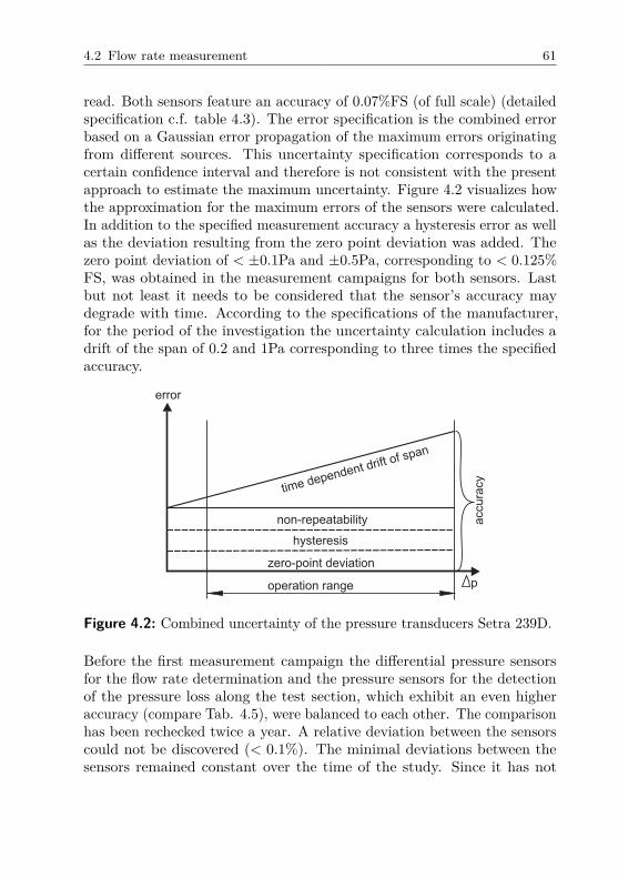
4.2 Flow rate measurement 61
read. Both sensors feature an accuracy of 0.07%FS (of full scale) (detailedspecification c.f. table 4.3). The error specification is the combined errorbased on a Gaussian error propagation of the maximum errors originatingfrom different sources. This uncertainty specification corresponds to acertain confidence interval and therefore is not consistent with the presentapproach to estimate the maximum uncertainty. Figure 4.2 visualizes howthe approximation for the maximum errors of the sensors were calculated.In addition to the specified measurement accuracy a hysteresis error as wellas the deviation resulting from the zero point deviation was added. Thezero point deviation of < ±0.1Pa and ±0.5Pa, corresponding to < 0.125%FS, was obtained in the measurement campaigns for both sensors. Lastbut not least it needs to be considered that the sensor’s accuracy maydegrade with time. According to the specifications of the manufacturer,for the period of the investigation the uncertainty calculation includes adrift of the span of 0.2 and 1Pa corresponding to three times the specifiedaccuracy.
error
p
zero-point deviation
non-repeatability
time dependent drift of span
hysteresis
operation range
accu
racy
Figure 4.2: Combined uncertainty of the pressure transducers Setra 239D.
Before the first measurement campaign the differential pressure sensorsfor the flow rate determination and the pressure sensors for the detectionof the pressure loss along the test section, which exhibit an even higheraccuracy (compare Tab. 4.5), were balanced to each other. The comparisonhas been rechecked twice a year. A relative deviation between the sensorscould not be discovered (< 0.1%). The minimal deviations between thesensors remained constant over the time of the study. Since it has not

62 4 Measurement uncertainty
Table 4.3: Product specifications Setra 239DSetra model 239Daccuracy RSS at constant temp. ±0.07% FSnon-linearity BFSL ±0.10% FShysteresis 0.10% FSnon-repeatability 0.02% FScompensated range ∘C −1 to +65
been possible to review the absolute errors by calibration, regardless anuncertainty due to time dependent drift of the span was added.
4.2.3 Fabrication tolerances
Fabrication tolerances play a role for nozzles and orifices, but differentparameters of the geometry are critical. In case of the nozzles the mainparameters are exact manufacturing of the inner diameter, the curvature atthe inlet and an accurate drilling of the pressure tab. Regarding the orificemeter, the disk itself can be purchased in high grade finish. In this casethe pipe is the inaccurate element, where the centering of the flanges ofthe intersections is important. In the present study the challenging aspectwere treated with special care, which is described in detail in Chapter 3.1.3.Fabrication tolerances are summarized in table 4.4.
At least the results for the 50mm and 74mm inlet nozzles were deviatingfrom expectations. The nozzles run with perfect reproducibility, but show asystematic deviation of the flow rate. This became obvious in the referencemeasurement for the channel in comparison to literature data. Thereforethe nozzles were calibrated with reference to the orifice meters (describedin Appendix A.1) and thus the accuracy is the same for both types ofinstruments. It is assumed that the deviation of the volume flux measuredby the nozzles results from an inaccurate fabrication of the inlet radius ofthe instruments. This is inconvenient regarding that the nozzles shouldnominally provide higher absolute accuracy than the orifice meters (seeSec. 4.3).

4.2 Flow rate measurement 63
Table 4.4: Manufacturing tolerances for the orifice meter run with theopening of orifice disk 𝑑 and the pipe diameter 𝐷
𝑑 [mm] 𝛿𝑑 [mm] 𝐷 [mm] 𝛿𝐷 [mm] 𝛽 𝛿𝛽
60 0.005 100.2 0.05 0.599 0.0003
4.2.4 Uncertainty of the calibration parameters
Uncertainties of the DIN-specified flow coefficients mainly result from thefact that the flow rate instruments are not calibrated in the particularinstallation situation. The norm specifies frame conditions for fabricationtolerances as well as conditions for the installation. Especially in the caseof the orifice meter run the uncertainty of the given calibration parametersmust include quite large tolerated deviations. In consequence the error fora certain flow instrument is primarily systematic, which implies that thereproducibility of the flow instruments is much better than the absoluteaccuracy.
Uncertainty of the calibration parameters includes the uncertainty of theflow coefficient 𝛼 (nozzle) or the orifice coefficient 𝐶 (orifice) (Eq.(3.2)and Eq. (3.3) in Chap. 3). Both have a major impact on the absolutemeasurement accuracy. The calculation is based on empirical formula thatcan again be found in the engineer standards (DIN24167-2 (nozzle) andDIN EN ISO 5167-1 (2003) (orifice)). In the present study the 50mm nozzlehas been calibrated to work at smaller flow rates. This tedious work andits unforeseen difficulties are described in Appendix A.1.
4.2.5 Combined uncertainty of flow rate measurement
The individual error sources are now added to a combined uncertainty ofthe flow rate measurement. The combined uncertainty will be presented asthe maximum error for the standard conditions defined in Table 2.1. Inthis way the estimate for the flow rate is equal to the uncertainty for themass flow ��, since the weighting of the density, which enters as squareroot in denominator for �� and in nominator for ��, is approximately thesame for the small uncertainty of the density calculation.
Figures 4.3 and 4.4 show the uncertainty of the flow rate for the nozzlesand for the orifice meters for different 𝐷 or 𝑑, respectively. For both types

64 4 Measurement uncertainty
0 50 100 150 200 2500
0.2
0.4
0.6
0.8
1
1.2
V [m3/h]
δ[%
]
max. uncertainty 50mm nozzlemax. non-reproducibility
(a)
0 100 200 300 400 5000
0.2
0.4
0.6
0.8
1
1.2
V [m3/h]
δ[%
]
max. uncertainty 74mm nozzlemax. non-reproducibility
(b)
Figure 4.3: Max. error of flow rate for nozzles with 𝐷 = 50mm (a) and𝐷 = 74mm (b).
As mentioned before, the fabricated nozzles did not comply with theintended geometry and were calibrated in reference to the orifice meters.Thus, the following considerations focus on the orifice meters.
Alternatively, a calculation of the uncertainty for �� can be derived fromthe norm DIN EN ISO 5167-1 (2003) for a 2𝜎 confidence interval.
𝛿��
��=
√(𝛿𝐶
𝐶
)2+
(𝛿𝑒
𝑒
)2+
(2𝛽4
1 − 𝛽4
)2 (𝛿𝐷
𝐷
)2
+(
21 − 𝛽4
)2 (𝛿𝑑
𝑑
)2+ 1
4
(𝛿Δ𝑝
Δ𝑝
)2+ 1
4
(𝛿𝜌
𝜌
)2.
(4.4)
of flow meters systematic errors are dominating, which mainly arise fromthe uncertainty of the flow coefficients and are larger for the orifice meter.The non-reproducibility 𝜖 is considerably better and almost identical forboth types of flow instruments. For the uncertainty as well as the non-reproducibility of the flow rate a peak originating from the switchingbetween the Setra sensors with different measurement ranges is clearlyvisible. One can deduce that the accuracy of the pressure transducers is ofmain impact for the reproducibility.

4.2 Flow rate measurement 65
0 50 100 150 200 2500
0.5
1
1.5
2
V [m3/h]
δ[%
]
max. uncertainty 60mm orificemax. non-reproducibility
(a)
0 100 200 300 4000
0.5
1
1.5
2
V [m3/h]
δ[%
]
max. uncertainty 75mm orificemax. non-reproducibility
(b)
Figure 4.4: Max. error of flow rate for orifice disks with 𝐷 = 60mm (a)and 𝐷 = 75mm (b).
This procedure is neither according to a Gaussian nor to a linear determi-nation of error propagation, since the calculation following DIN EN ISO5167-1 (2003) equally handles statistical and systematic errors by accu-mulating the modulus using a weighting of the single error contributions.In particular, the weighting of the uncertainty arising from differentialpressure measurement is not plausible to the author. It leads to a verysmall influence of the pressure measurement on the combined uncertaintyas exemplarily shown in Figure 4.5. Thus, instead of using the uncertaintyconsideration according to DIN, linear error propagation is used for theestimation of uncertainties. Nonetheless, in the present case the procedureaccording to DIN delivers approximately the same result as the linear errorpropagation.
4.2.6 Uncertainty of Reynolds number in the test section
If we consider the uncertainty of the Reynolds number in the test sectionbased on equation (4.5) and insert the flow rate, four potential error sourcesaffecting 𝑅𝑒𝑏 are identified:
∙ viscosity,
∙ tolerances of the test section geometry,
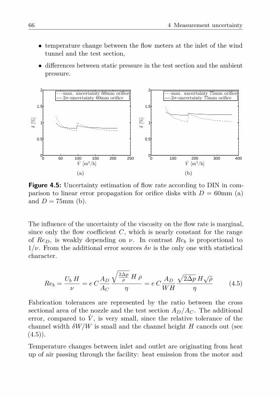
66 4 Measurement uncertainty
0 50 100 150 200 2500
0.5
1
1.5
2
V [m3/h]
δ[%
]
max. uncertainty 60mm orifice2σ-uncertainty 60mm orifice
(a)
0 100 200 300 4000
0.5
1
1.5
2
V [m3/h]
δ[%
]
max. uncertainty 75mm orifice2σ-uncertainty 75mm orifice
(b)
Figure 4.5: Uncertainty estimation of flow rate according to DIN in com-parison to linear error propagation for orifice disks with 𝐷 = 60mm (a)and 𝐷 = 75mm (b).
The influence of the uncertainty of the viscosity on the flow rate is marginal,since only the flow coefficient 𝐶, which is nearly constant for the rangeof 𝑅𝑒𝐷, is weakly depending on 𝜈. In contrast 𝑅𝑒𝑏 is proportional to1/𝜈. From the additional error sources 𝛿𝜈 is the only one with statisticalcharacter.
𝑅𝑒𝑏 = 𝑈𝑏 𝐻
𝜈= 𝑒 𝐶
𝐴𝐷
𝐴𝐶
√2Δ𝑝
𝜌 𝐻 𝜌
𝜂= 𝑒 𝐶
𝐴𝐷
𝑊𝐻
√2Δ𝑝 𝐻
√𝜌
𝜂(4.5)
Fabrication tolerances are represented by the ratio between the crosssectional area of the nozzle and the test section 𝐴𝐷/𝐴𝐶 . The additionalerror, compared to �� , is very small, since the relative tolerance of thechannel width 𝛿𝑊/𝑊 is small and the channel height 𝐻 cancels out (see(4.5)).
Temperature changes between inlet and outlet are originating from heatup of air passing through the facility: heat emission from the motor and
∙ temperature change between the flow meters at the inlet of the windtunnel and the test section,
∙ differences between static pressure in the test section and the ambientpressure.

4.2 Flow rate measurement 67
dissipative losses (skin-friction, Borda-Carnot losses). All dissipative losseslead to a temperature increase of the fluid with the exception of the Borda-Carnot loss at the outlet. The arising pressure drop losses need to becompensated by the ventilator, which is producing additional heat emissionin dependence of the power consumption and the efficiency. A theoreticalcalculation including the previously mentioned heat sources, indicated verysmall influence for small 𝑅𝑒𝑏. The heat-up of the fluid has been computedto estimate the difference between inlet and outlet temperature Δ𝑇 shownin Figure 4.6. To confirm the theoretical consideration, measurement datafrom the temperature difference between inlet and outlet for stationaryoperating mode are added to the plot. Measurement and computation forthe 74mm inlet nozzle are in very good agreement. If we use the meanvalue of inlet and outlet temperature for the calculation of �� as well as of𝑅𝑒𝑏, the resulting error in the temperature is smaller than the error 𝛿𝑇we estimated for low 𝑅𝑒𝑏. For 𝑅𝑒𝑏 > 18000, we have a low impact andneed to determine �� and 𝑅𝑒𝑏 based on different ambient temperatures. Inthe present case the temperature increase within the test section is lowcompared to the other heat sources of the system (< 15%). Thus thetemperature in the test section can be regarded constant. The validity ofthis assumption is also limited to the moderate 𝑅𝑒𝑏 of the present study.
Figure 4.6: Difference between inlet and outlet temperature (calculationof 𝑅𝑒𝑏 based on mean temperature).
Regarding the static pressure at the flow rate instruments, the marginalpressure loss to the location of the pressure tab is automatically included

68 4 Measurement uncertainty
in the DIN-calibration for the nozzles. For the orifice meters the staticpressure in the pipe in the proximity of the orifice disk is almost equal tothe barometric pressure due to the comparably low velocities in the pipe(restricted by the range of the Setra sensors Δ𝑝𝑚𝑎𝑥 = 625Pa).
The static pressure at the channel inlet is the overpressure of the settlingchamber, which is driving the flow. The pressure decreases due to energydissipation along the test section and is equal to the barometric 𝑝 = 𝑝𝑏𝑎𝑟
at the outlet of the test section. Figure 4.7 shows the pressure differencefrom channel inlet to the outlet based on the assumption of the validityDean’s law for the whole channel. If we consider the overpressure for thecomplete test section, this effect is definitely negligible for 𝑅𝑒𝑏 < 23000.In this operational range the changes of temperature and static pressureare negligible small in the channel, which is essential for the validity of thecriterion of constant density. If the channel section works at 𝑅𝑒𝑏 > 30000these effects will become relevant. Note that in this case 𝑅𝑒𝑏 would slightlychange along the channel.
Figure 4.7: Estimation of the pressure loss in the test section according toDean’s law.
As a result of the preceding analysis, the error graph for 𝑅𝑒𝑏 in Figure4.8 is very similar to the one for �� , since the viscosity and the fabricationtolerances bring very small additional errors.

4.3 Determination of pressure drop along the test section 69
0 2500 5000 7500 10000 12500 150000
0.5
1
1.5
2
Reb
δ[%
]
max. uncertainty 60mm orificemax. non-reproducibility
(a)
0 5000 10000 15000 20000 250000
0.5
1
1.5
2
Reb
δ[%
]
max. uncertainty 75mm orificemax. non-reproducibility
(b)
Figure 4.8: Max. error of 𝑅𝑒𝑏 for orifice disks with 𝐷 = 60mm (a) and𝐷 = 75mm (b).
4.3 Determination of pressure dropalong the test section
For the measurement of the pressure evolution along the test section, twoerror sources need to be considered: on the one hand a possible deviationoriginating from the pressure taps and on the other hand the accuracy ofthe differential pressure sensors.
While common pressure sensors exhibit an accuracy of ±0.1 − 0.5 % FS,the two Baratron 696A sensors offer ±0.12% R (of reading) in three mea-surement ranges. Even smallest values can be detected with the highestaccuracy. In order to obtain the most accurate results possible, the mea-surement range of the sensor needs to be adjusted to the expected pressurelosses. Baratron sensors are temperature compensated and after a certainheat-up time of a few days show minimal dependency of the zero pointon the ambient temperature. The drift of the zero point is compensatedmanually with an accuracy of ±0.01Pa for all ranges. It has been done soand minuted for every measurement day.
Disadvantages of the Baratron sensors should not be omitted here. Thelow temporal resolution of 10Hz limits the application to more or lessstationary flows. Concerning the present work this is not a constraint, sincedynamic processes are not examined using pressure measurement technique.Detailed specifications of the Baratron sensors are found in Table 4.5.

70 4 Measurement uncertainty
Table 4.5: Specifivations of differential pressure sensors MKS Baratron698A
Specifications of type 698𝐴
accuracy 0.12% of reading ± zero/Span coeff.full scale pressure ranges (Torr) 1, 10resolution (FS) 1 × 10⁻⁶
sensor temperature regulated at 45∘Ctemperature effects on span < 0.002% R / ∘C (20ppm)temperature effects on zero < 15 PPM, FS /∘Ctype of measurement differentialuseable resolution 5 decades
The producer MKS calibrates the devices to less than half the error of a3𝜎-confidence interval, which is proven by a calibration certificate. Thisspecification is assumed to be in accordance to the present uncertaintycalculation.
The pressure taps were analyzed following Tropea et al. (2007) with respectto potential errors originating from:
∙ the tap diameter,
∙ the relative tapping depth,
∙ the condition of the tapping orifice.
The tap diameter is of major importance, since all other potential errorsare highly dependent on this parameter. Therefore the tap diameter waschosen small with only 0.3mm and taps were manufactured in high quality.If the tap diameter is normalized by the viscous length scale 𝛿𝜈 , we obtain𝑑+
𝑡𝑎𝑝 < 15 for the riblet study. For all other studies it is considerably smaller(𝑑+
𝑡𝑎𝑝 < 10). Due to the small diameter, the errors are negligible (𝛿 ≪ 0.1%)with respect to all mentioned aspects.

4.3 Determination of pressure drop along the test section 71
0 2000 4000 6000 8000 10000 12000 140000
0.5
1
1.5
2
2.5
3
3.5
Reb
δ[%
]
δcfmax
ǫcfmax
(a)
0 4000 8000 12000 16000 20000 240000
0.5
1
1.5
2
2.5
3
3.5
Reb
δ[%
]
δcfmax
ǫcfmax
(b)
Figure 4.9: Max. error and non-reproducibility of 𝑐𝑓 for orifice disks with𝐷 = 60mm (a) and 𝐷 = 75mm (b).
4.3.1 Uncertainty of friction coefficient
The only further source of error affecting the friction coefficient is thepressure drop along the test section as can be obtained from:
𝑐𝑓 = Δ𝑝𝑙𝐻
𝜌𝑐 𝑈2𝑏 𝐿
= Δ𝑝𝑙𝐻
𝜌𝑐(𝑒 𝐶 𝐴𝐷
𝐴𝐶
√2Δ𝑝𝑓
𝜌𝑓)2𝐿
for 𝜌𝑐 = 𝜌𝑓 = 𝜌 : 𝑐𝑓 = Δ𝑝𝑙𝐻
(𝑒 𝐶 𝐴𝐷
𝐴𝐶)22Δ𝑝𝑓 𝐿
.
(4.6)
As shown in the previous section the uncertainty of the pressure drop issmall compared to the uncertainty of the flow rate. Thus the main impactresults from the quadratic relation on 𝑈𝑏. The influence of fabricationtolerances grows, since now the channel height 𝐻 does not vanish. Forexample a deviation of 0.25mm would lead to an error of 1% in 𝑈𝑏. However,the fabrication tolerances are fare less for the present set-up (cf. Chapter3.2) If differences in the density between the location of flow rate meter𝜌𝑓 and the channel section 𝜌𝑐 - basically induced by temperature increaseand large overpressure in the test section at high 𝑅𝑒𝑏 - are neglected, asystematic linear error dependency is obtained. Note that as long as the

72 4 Measurement uncertainty
0 2000 4000 6000 8000 10000 12000 140000
0.5
1
1.5
2
2.5
3
3.5
Reb
δcf[%
]
SetraBaratronCβ
other
(a)
0 5000 10000 15000 200000
0.5
1
1.5
2
2.5
3
3.5
Reb
δcf[%
]
SetraBaratronCβ
other
(b)
Figure 4.10: Max. error of 𝑐𝑓 split into error sources for orifice disks with𝐷 = 60mm (a) and 𝐷 = 75mm (b).
In literature the uncertainty of the instrument for skin-friction detection iscommonly given, while the effect of flow rate uncertainty is not taken intoaccount, although its impact on the data is generally larger than the errorof the pressure measurement.
assumption of a nearly constant density through the facility holds, 𝑐𝑓 doesnot depend on 𝜌 (see Eq. (4.6).
Assuming a quadratic relation between the flow velocity 𝑈𝑏 and the pressureloss in the channel, a variation of the flow rate has twice the impact onthe pressure loss. If this is transferred to a plot of 𝑐𝑓 versus 𝑅𝑒𝑏, the errorof the flow rate determination on the abscissa affects the values on theordinate of the 𝑐𝑓 -value by factor two.
In Figure 4.9 the bias and random errors are distinguished. It is clearlyvisible that a large portion relates to systematic errors. Thus reproducibilityof 𝑐𝑓 is fairly good. Figure 4.10 splits the total uncertainty of the frictioncoefficient into the individual error sources: the pressure sensors for Δ𝑝𝑓
and Δ𝑝𝑙, 𝐶, 𝛽 and others. The major part of the uncertainty results fromthe flow coefficient 𝐶, which represents a pure systematic uncertainty. Thelarger absolute uncertainty of the 75mm disk is a result of 𝛿𝐶 increasingwith 𝛽. Obviously a calibration of the flow meter could reduce the absoluteuncertainty by one half.
4.3 Determination of pressure drop along the test section 73
4.3.2 Determination of skin friction changes independence of the measurement strategy
The experimental set-up has to provide an accurate information aboutthe difference in skin-friction between a smooth reference and test case.For that purpose the absolute accuracy is not the limiting condition butthe reproducibility, since systematic errors in the measurement do notalter the ratio 𝜏𝑤/𝜏𝑤,0 = 𝑐𝑓 /𝑐𝑓,0 (Fig. 4.11 (1) and (2)). Thus the non-reproducibility of the pressure sensors for flow rate as well as for detection ofpressure drop along the channel and the sensors for the ambient parametersare the crucial issues. The largest identified source of uncertainty wasthe one related to the flow coefficient 𝐶, which does not affect the result.Nevertheless, the flow rate contributes the largest error to the measurementas illustrated by the horizontal error bar in Figure 4.11. If in the worstcase the computation of 𝜏𝑤/𝜏𝑤,0 is based on two data points, one for testsurface and one for the reference, the non-reproducibilities add and resultin quite large uncertainty. The confidence can be improved, if a test seriesis repeated several times and then averaged, as done in the present study(Fig. 4.11 (3)). Then reproduction errors are statistically distributed and aGaussian distribution can be assumed. The error propagation law accordingto Gauß can be applied. The average of the data and a confidence interval𝜎 is computed (4). If we employ a confidence interval of 1𝜎, the uncertaintyfor a comparison of the test and reference measurement can be determined.Expecting identical standard deviation for both cases, the uncertainty willpropagate as:
𝛿1𝜎 =√
𝜎20 + 𝜎2
𝑡𝑒𝑠𝑡 =√
2𝜎. (4.7)
Two factors can improve the accuracy of the measurement: The first is thetime dependence of the reproduction error. Part of the previously discussederrors originates from deviations of the sensors with time, which can alsobe random. For example the zero point deviation of the Setra sensors didnot show a specific preference in time, but varied in both directions. Ina measurement campaign which took weeks or months, the deviation wasobserved to be statistically distributed, but was approximately constantwithin one day. If a test series can be conducted within one day the datascatter is be minimized and the accuracy of 𝜏𝑤/𝜏𝑤,0 is increased.

74 4 Measurement uncertainty
cfuncertainty
reference
testsurface
non-reproducibility
measurementdata
maximumerror
Reb
averagevalue
s
s
standarddeviation
(1) (2) (3) (4)
Figure 4.11: Influence of the uncertainty on the significance of the data.
The second and essential factor is the strategy of testing. Figure 4.12schematically visualized the maximum error occurring from the the strategyon base of a single measurement. The major impact on non-reproducibility𝜖 of 𝑐𝑓 originates from the flow rate measurement, which is symbolized bythe horizontal error bar, since 𝜖𝑐𝑓 is quadratically proportional to 𝑈𝑏.
cf non-reproducibility
maximumerror
Reb
non-reproducibility
dominatingvertical error
Reb
tw,0
tw
0
Figure 4.12: Strategy 1: comparison of reference and test case from separatemeasurements.
As Figure 4.13 illustrates, the situation changes if the measurement of testand reference conditions can be conducted simultaneously. For examplein a long channel there can be two segments, one with a smooth referencesurface and one with a modified surface condition. In this case the flow ratemust definitely be same for both surface conditions. All errors arising fromthe flow rate posses the same magnitude and sign. The consequence is a lowinfluence of the flow rate uncertainty to the amount of 𝜏𝑤/𝜏𝑤,0. Nonethelessscatter will be visible in the data, when repeating the measurement. In

4.3 Determination of pressure drop along the test section 75
fact 𝜏𝑤/𝜏𝑤,0 is quite exactly known, but the horizontal position of a datapoint is still affected by the non-reproducibility of the flow rate.
cf non-reproducibility
same sign ofstatistical error
Reb
non-reproducibility
error mainlyhorizontal
Reb
tw,0
tw
reduction ofvertical error
0
Figure 4.13: Strategy 2: comparison of reference and test case within thesame test run.
During the measurement campaigns different strategies will be utilized togain the most accurate result in the particular constellation. In generalit is beneficial to enable a direct comparison to the reference. In mostcases measurement of reference and test case are conducted at differenttimes. The time inbetween leads to larger scatter in the data, sinceinfluence of deviations in the sensors is present. The present uncertaintyestimation includes these aspect for �� , 𝑅𝑒𝑏 and 𝑐𝑓 . Although the absoluteaccuracy is stated to be the same for all studies, the non-reproducibilitywill differ significantly depending on the measurement strategy, because themeasurement strategy essentially influences the magnitude of the statisticalerrors.
Changes in the ambient temperature, pressure or humidity are small consid-ering a single measurement or even one day of tests. Temperature changeswere smaller than 0.3∘C per hour, maximum variation in the barometricpressure has been Δ𝑝𝑚𝑎𝑥 < 1 hPa/h. If a test run did not satisfy thesecriteria, it was not taken into account in the investigation. Note that inall studies conducted in the present work, except for the investigation ondielectric electro-active polymers, any test run needs to be related to areference data set. Both data sets consist of 20 pressure measurementsand all need to be related to one 𝑅𝑒𝑏 to enable a comparison of the two.Otherwise the reproducibility would limit the identification of small changesin skin-friction between the test cases. Therefore, the ambient values of𝑇, 𝑝 and, if available, ℎ were minutely documented for every single set ofmeasurement.
76 4 Measurement uncertainty
4.4 Steadiness of the flow
Differences in reproduced data result not only from the non-repeatability ofthe flow rate measurement or the measurement of the pressure loss, but alsodepend on steadiness of the flow rate. If the wind tunnel does not produceexactly the same flow rate over the time of measurement this can have acertain influence. At first sight the steadiness should have no impact on theaccuracy, since a deviation in 𝑅𝑒𝑏 will cause a corresponding deviation inΔ𝑝. It may thus not be possible to exactly reach a certain 𝑅𝑒𝑏 but all datashould match the curve 𝑐𝑓 = 𝑓(𝑅𝑒𝑏). Now if a measurement of a singletab is conducted, the effect may be without impact. In the case of a seriesof readings to determine a distribution along the channel, the Reynoldsnumber can slightly change with time. In consequence, any single datapoint of the data corresponds to a slightly different 𝑅𝑒𝑏 and plotting thedevelopment of the flow along the channel can show considerable scatter.The question arises how long one pressure tab needs to be recorded to avoidthe time-dependence. To answer this question, the flow rate in the facilityis measured over 10min, which is estimated to be long enough to obtain𝑐𝑓 = 𝑓(𝑡). During the measurement the ambient parameters are reviewedto be exactly constant. The 10min-interval is then split into defined timeperiods to compare the mean value of each section to the 10min-average.Exemplarily for a time step of 1min, we get 10 intervals and identify theone with the largest deviation. As the steadiness is depending on 𝑅𝑒𝑏 ameasurement for different flow rates is required to represent the full 𝑅𝑒𝑏-range. In Figure 4.14 the results for the turbulent flow conditions of threeminutes intervals is shown (13% tripping, see Chap. 5). For 𝑅𝑒𝑏 > 8000the influence is extremely small, but it slightly grows for lower 𝑅𝑒𝑏. Thedeviations is still smaller 0.1% even for 𝑅𝑒𝑏 = 2700, which corresponds tothe transitional regime. Thus a recording time of 3min was found to beadequate to exclude time dependence.
There is another aspect of time-dependent fluctuations of the flow leftout by the consideration so far: the interaction of the tunnel and the testsection. If the friction value in the test section is not constant, the ventilatorhas to deal with varying pressure losses and the wind tunnel control needs

4.4 Steadiness of the flow 77
0 2000 4000 6000 8000 10000 12000 140000
0.02
0.04
0.06
0.08
0.1
Reb
∆Re[%
]
Figure 4.14: Deviation of 3min minutes sequences of a 10min measurementof the Reynolds number.
to react to keep the flow rate constant. For laminar as well as for turbulentflow this effect is negligible, but for transitional flow conditions the windtunnel control becomes a key parameter. In the present study very goodresults have been achieved by setting the tunnel control to simply keepthe rotation rate constant. The described effect should not be confusedwith the data scatter in the transitional region. The transitional regimenaturally contains fluctuations of the pressure losses for the same flow rate,which can not be filtered out by increasing the integration time and evenis not an result of the tunnel control. This random unsteadiness is partof the transitional flow behavior and cannot be considered a measurementerror.


5 Reference measurement
The present Chapter considers the measurement results obtained witha smooth surface in the test section. The main goal of the Chapter isto generate a reference data set for the smooth surface, which is to becompared with literature data. Two fundamentally different flow conditionsare investigated:
∙ naturally developing channel flow
∙ artificially generated turbulent channel flow.
The naturally developing flow is the important reference for laminar andtransitional flow control. Throughout the Chapter data with focus onthe transitional range of 𝑅𝑒 is presented. These data of the flow will beexploited for the reference case in Chapter 7.
The artificial generation of turbulence aims at producing a fully developedflow at rather small Reynolds numbers. In such a range of Reynoldsnumbers, the flow would naturally be laminar or transitional. Consideringsurface morphology that has shown to be effective for reducing skin frictionin turbulent air flows, the physical dimensions of the surface structure werefound to be quite small and to decrease with increasing 𝑅𝑒. Thereforeit is particularly beneficial to work at low Reynolds numbers to avoid aReynolds number range were fabrication tolerances would influence theresults. This demands for initiating transition to turbulence at low 𝑅𝑒. Dueto the care, which has been taken to achieve undisturbed flow conditionsfor laminar investigations, artificial tripping is essential to enable transitionto turbulence at low 𝑅𝑒. On the one hand, the flow is forced to be fullyturbulent at low flow velocities and on the other hand the developmentlength is shortened.
For both approaches hot-wire-instrumentation is used to determine the flowstate at the channel outlet and is complemented with the results observedwith the pressure tap measurement along the channel. The latter providesinformation about the flow development and the skin-friction. Comparison

80 5 Reference measurement
with literature data and theoretical predictions introduced in Chapter 2 isprovided.
Furthermore, three of the initial assumptions require experimental exami-nation:
∙ the deviation from an ideal two-dimensional flow
∙ the development length in the turbulent case
∙ the verification of a hydraulically smooth surface.
The development length is investigated and compared with literature datafor turbulent and laminar flow.
The reference measurement will indicate whether the hydraulic smoothcondition is justified with 𝑅𝑎 = 0.4𝜇m. Good agreement with the solutionfor smooth plates is expected since surface roughness is 10 times smallerthan the strict criterion for turbulent flows obtained from Gruneberger’sinvestigation (Gruneberger & Hage, 2011).
The first two aforementioned aspects are clarified through the presentationof the reference data. The quantification of the spanwise distributionof velocity and skin friction demands for an introduction of a specialmeasurement technique, the Preston tube, and is separately presented atthe end of this Chapter.
5.1 Naturally developing flow
The measurements for laminar and transitional flows are presented in moredetail by Schickel (2012). Only a short summary will be given in thissection introducing the main aspects of the solid reference case. Since inthe meantime a calibration of the 50mm-nozzle, which was used for the flowrate measurement by Schickel (2012), enabled a more accurate computationof the flow rate, the data were replotted.
First we study the turbulence level 𝑇𝑢 in the channel in dependenceof 𝑅𝑒𝑏 using a hot-wire installed approximately 70mm upstream of the

5.1 Naturally developing flow 81
channel outlet. All hot-wire measurements were conducted with a DantecStreamline system. Utilizing the formula
𝑇𝑢 =
√𝑢2
𝑈∼=
4𝐸
𝐸2 − 𝐸0
2
√𝑒2, (5.1)
which is derived in Appendix A.2, allows to directly compute 𝑇𝑢 fromthe voltage output 𝐸 of the anemometer. In the formula 𝐸 is the timeaverage of the voltage, 𝐸0 the voltage output with resting fluid and
√𝑒2
the RMS-value. The major advantage of this procedure is the avoidance oftime-consuming hot-wire calibrations.
0 2000 4000 6000 8000 10000 12000 140000
2
4
6
8
10
12
14
Reb
Tu[%
]
decreasing flow rateincreasing flow rate
Figure 5.1: Turbulence level in naturally developing channel flow in depen-dence of 𝑅𝑒𝑏 for increasing and decreasing flow rate.
Figure 5.1 shows the turbulence level in dependence of the Reynolds numberfor increasing and decreasing 𝑅𝑒𝑏. The flow rate has been changed in verysmall steps to exclude affecting the flow state by acceleration or variationof the flow rate. As can be observed at low 𝑅𝑒𝑏 the turbulence level issmall, indicating laminar flow. It abruptly increases when reaching thetransitional flow state at approximately 𝑅𝑒𝑏 = 6000 for increasing flow rate.In the fully turbulent state the turbulence level asymptotically approachesto 𝑇𝑢 ≈ 4% for 𝑅𝑒𝑏 > 7000 which agrees with the results of Durst et al.
82 5 Reference measurement
(1998). For decreasing flow rate the transition region is slightly shifted tosmaller 𝑅𝑒𝑏. This behavior is typical for naturally developing flow and wasobserved by Jovanovic et al. (2011) in the same range of 𝑅𝑒.
If we regard the flow development in the channel for different 𝑅𝑒𝑏 (Figure5.2 (a-f)) different streamwise developments of the flow are observed. Forlow Reynolds numbers (a) and (b) a rather constant slope is reached atthe channel outlet. At higher 𝑅𝑒𝑏 the development length increases andexceeds the length of the tunnel. The onset of transition in the downstreampart of the channel at 𝑅𝑒𝑏 = 6190 (c) can clearly be noticed from thepressure distribution. The onset of transition results in an inflection pointin streamwise distribution of Δ𝑝, which moves upstream with increasing𝑅𝑒𝑏 (d-f). At 𝑅𝑒 = 12800 (f) transition to turbulence is still observed overa considerable length of the channel.
In Figure 5.3 the pressure loss of the experimental data for the completelength of the test section are compared with the theoretical prediction forlaminar developing flow by Schlichting (1934), which has been introducedin Chapter 2.2.2. Since measurements by Durst et al. (2005) proved thatthe development length is slightly longer than Schlichting’s prediction(see Fig. 5.4), the result from the theory has been modified for a 5%longer development length in Figure 5.3. Although the theory is based ona two-dimensional theory, the agreement is rather good. If one acceptsSchlichting’s approach, assuming a centerline velocity deviating 2% fromthe value of the parabolic profile to be negligible, we can compute thedevelopment length. The result is plotted in Figure 5.4. Additionally,for four marked points in Figure 5.4, the corresponding pressure lossmeasurement are shown in Figure 5.5(a-d). In these plots the analyticsolution 𝑐𝑓 = 12/𝑅𝑒𝑏 is included by straight lines and is compared withthe slope of the pressure drop at the channel outlet: The length of thechannel is not sufficient to fully develop the flow for 𝑅𝑒𝑏 > 3600.
Complementary, Figure 5.6 shows the mean value of the friction coefficientfor the complete test section (a) and the downstream segment (b) of testsection. The transitional region can be clearly identified by a large increaseof 𝑐𝑓 in both plots. Since (b) shows larger values of 𝑐𝑓 for the completeturbulent range, the persistence of a distinct fraction of laminar flow in thechannel is confirmed even for highest 𝑅𝑒𝑏. The comparison to Dean’s lawin the downstream section in (b) indicates that for the highest 𝑅𝑒𝑏 a fullydeveloped state is achieved in the downstream segment. In the laminarregime is it clearly visible that the measurement data departs from the

5.1 Naturally developing flow 83
0 1 2 3 40
1
2
3
4
5
6
x [m]
∆pl[P
a]
(a) 𝑅𝑒𝑏 = 4250
0 1 2 3 40
2
4
6
8
10
x [m]
∆pl[P
a]
(b) 𝑅𝑒𝑏 = 5820
0 1 2 3 40
2
4
6
8
10
12
14
x [m]
∆pl[P
a]
(c) 𝑅𝑒𝑏 = 6190
0 1 2 3 40
5
10
15
20
25
30
x [m]
∆pl[P
a]
(d) 𝑅𝑒𝑏 = 8180
0 1 2 3 40
10
20
30
40
x [m]
∆pl[P
a]
(e) 𝑅𝑒𝑏 = 10000
0 1 2 3 40
10
20
30
40
50
60
70
x [m]
∆pl[P
a]
(f) 𝑅𝑒𝑏 = 12800
Figure 5.2: Streamwise distribution of the static pressure in the test sectionfor different 𝑅𝑒𝑏.

84 5 Reference measurement
0 2000 4000 6000 80000
5
10
15
20
25
30
Reb
∆pl[P
a]
Schlichting
Figure 5.3: Comparison of a theoretical channel entrance (Schlichting(1934)) flow with the measured pressure loss distribution.
0 1000 2000 3000 4000 5000 6000 70000
1
2
3
4
5
6
7
Reb
LE[m
]
LE Durst et alLE Schlichting
Figure 5.4: Development length of a laminar channel flow calculated forthe dimensions of the present channel according to Schlichting (1934) andDurst et al. (2005). Circles denote measurement points depicted in Figure5.5.

5.1 Naturally developing flow 85
LE
Du
rst
et
al.
(20
05
)
(a) 𝑅𝑒𝑏 = 2950
LE
Du
rst
et
al.
(20
05
)
(b) 𝑅𝑒𝑏 = 3530
0 1 2 3 40
1
2
3
4
5
6
x [m]
∆pl[Pa]
measurement datashiftedanalytic solution
(c) 𝑅𝑒𝑏 = 4590
0 1 2 3 40
1
2
3
4
5
6
7
x [m]
∆pl[Pa]
measurement datashiftedanalytic solution
(d) 𝑅𝑒𝑏 = 4970
Figure 5.5: Streamwise development of laminar flow at different 𝑅𝑒𝑏.Dashed lines mark the development length 𝐿𝐸 according to Durst et al.(2005) in (a) and (b).

86 5 Reference measurement
0 2000 4000 6000 8000 10000 120002
3
4
5
6
7
8
x 10−3
Reb
cf
(a)
0 2000 4000 6000 8000 10000 120002
3
4
5
6
7
8
x 10−3
Reb
c f
Dean‘s law12/Re
(b)
Figure 5.6: Friction coefficient calculated for the total length (a) and thedownstream segment (b)
analytical solution with increasing 𝑅𝑒𝑏, which is not surprising since therunning length is not sufficient for a full development as seen before.
Note that in all diagrams of the naturally developing flow the pressure tapat 2m is obviously working imperfectly. Since the deviation is small andreproducible, the obtained information is still valuable for the investiga-tions.
Finally, we inspect the data of the natural flow development in Figures 5.2and 5.5 with respect to disturbances at the intersections of the channelplates at 0.95m and 2.45m. There is no indication that the transition istriggered by imperfections at the intersections for any value of 𝑅𝑒.

5.2 Artificially generated turbulent flow 87
5.2 Artificially generated turbulent flow
In comparison with the previously presented study of naturally developingflow, the set-up has been modified in two significant details:
∙ Two Baratron sensors measure the pressure along the test section,which almost saves half of the time. The pressure taps at the firstand middle position are read by both sensors simultaneously to detectpotential deviations between the devices.
∙ The temperature measurement has been improved and the humidityis considered for the studies of riblets and dielectric electro-activepolymer actuators.
Different tripping has been tested to achieve turbulent flow for lowest 𝑅𝑒.The turbulence level has been measured for 12%, 13% and 16% blockageof the cross sectional area. Each tripping device was made from a 0.35mmthin brass section and installed at the top and bottom wall directly afterthe contraction in the tunnel entrance.
Figures 5.7 and 5.8 show the corresponding results for the turbulencelevel measured with a hot-wire at the end of the channel and the frictioncoefficient for the last section of the channel (𝑥 > 100𝐻), where thedevelopment length can be assumed sufficient for turbulent conditions (c.f.Chap. 2.2.2).
Figure 5.7 (a) shows the turbulence level for the 13% tripping. Transitionis observed at approximately 𝑅𝑒𝑏 = 2300. The hot-wire measurementsindicate that a fully turbulent flow at the outlet develops at 𝑅𝑒𝑏 = 3500. InFigure 5.7 (b) the friction coefficient for the last segment of the channel forthe same Reynolds number range is illustrated. The comparison to Dean’slaw (line) implies that a fully developed state is reached for 𝑅𝑒 > 3500−3800on the last segment, which corresponds to higher flow rate than desired.With 12% blockage (not shown) the result is similar; both the transition aswell as the agreement to Dean is shifted to even higher Reynolds number(Δ𝑅𝑒𝑏 = 200). Thus the tripping was increased to 16%, which leads toturbulent flow at even smallest 𝑅𝑒𝑏 (Fig. 5.8(a)). This is confirmed bythe good agreement to Dean on the last segment (b). Yet, a disadvantageat the high tripping level has been observed. The large tripping devicedoes not only affect the boundary layers of the developing flow and triggerstransition, it also causes large fluctuations in the static pressure. This canbe interpreted as a phenomena similar to the flow downstream an orifice

88 5 Reference measurement
0 2000 4000 6000 8000 10000 120000
5
10
15
Reb
Tu[%
]
increasing flow ratedecreasing flow rate
(a) (b)
Figure 5.7: Turbulence level at the channel end (a) and friction coefficientover 𝑅𝑒𝑏 on the downstream segment (b) for the tripping with 13% blockage.In (b) Dean’s correlation is compared with the data and uncertainty intervalsdeduced in Chapter 4.3.1 are shaded in grey.
0 2000 4000 6000 8000 10000 120002
4
6
8
10
Reb
Tu[%
]
increasing flow ratedecreasing flow rate
(a) (b)
Figure 5.8: Turbulence level at the channel end (a) and friction coefficientover 𝑅𝑒𝑏 on the downstream segment (b) for the tripping with 16% blockage.In (b) Dean’s correlation is compared with the data and uncertainty intervalsare shaded in grey.

5.2 Artificially generated turbulent flow 89
disk in a pipe, where a wake region with large vortex structures persistsover a long streamwise distance. In Figure 5.10 (b), where the 𝑐𝑓 -valuefor the entrance region (based on the differential pressure at the secondtap 𝑥 = 0.3m) is depicted, the resulting large scatter in the data can beobserved for small 𝑅𝑒𝑏. In (Fig. 5.8) (b) additionally the uncertaintyintervals (grey shaded) are compared with the measurement data. If weconsider, that the bias error of 𝑐𝑓 was estimated to be larger than 50%of the maximum uncertainty (compare Chap. 4.3.1), the obtained scatter(random error) in case of the 16% tripping significantly exceeds the errorcalculation for 𝑅𝑒 < 4500. This obviously confirms the “orifice” effect andled to the decision to work with a smaller tripping level.
While for the 13% tripping in Figure 5.7 (b) for turbulent flow the agreementwith the experimental literature data is very good, a small deviation fromthe analytical solution for laminar flow 𝑐𝑓 = 12/𝑅𝑒𝑏 is obtained. Thereare three potential sources why the 𝑐𝑓 of the channel is slightly higherthan the analytical solution at low 𝑅𝑒 (𝑅𝑒𝑏 < 2500) in Figure 5.7(b). Thefirst is the development of the flow, where a fully developed flow stateis not completely accomplished and can lead to slightly higher Δ𝑝𝑙 andconsequently 𝑐𝑓 . The second and estimated to be the dominant influenceis the deviation from a two dimensional flow state. The third reason isthe disturbance created by the tripping, which may not have dissipatedcompletely, thus generating some higher friction. However, this influence isprobably negligible in the second half of the channel.
The region of increased scatter between 3800 < 𝑅𝑒𝑏 < 4400 results fromcharacteristics of the 50mm-nozzle at low flow rates, which was identifiedafter the campaign and is discussed in Appendix A.1. The increased scatterbasically results from transition in the nozzle. The mean value is notaffected, while the scatter is approximately twice. Therefore, the orificemeter was used for later measurements with 13% tripping, as in the caseof the riblet and the dielectric elastomer actuator studies. Nevertheless,the results for the first generation of the instrumentation show less scatterthan most of the available literature data, but the benefit of the recentevolution is clearly visible in Figure 5.11.
The 13% blockage is considered to be the best compromise between shiftingthe fully developed turbulent flow to lower 𝑅𝑒 and introducing large scaledisturbances. Therefore, it is chosen for tests in the studies presented inChapters 6 to 8. In the following the discussion of the flow developmentwill focus on this configuration.

90 5 Reference measurement
0 1 2 3 40
0.5
1
1.5
2
2.5
3
x [m]
∆pl[Pa]
Sensor 1Sensor 2
(a) 𝑅𝑒𝑏 = 2420
0 1 2 3 40
1
2
3
4
5
x [m]
∆pl[Pa]
Sensor 1Sensor 2
(b) 𝑅𝑒𝑏 = 2800
0 1 2 3 40
2
4
6
8
10
12
14
x [m]
∆pl[Pa]
Sensor 1Sensor 2
(c) 𝑅𝑒𝑏 = 4790 (d) 𝑅𝑒𝑏 = 7620
(e) 𝑅𝑒𝑏 = 9730 (f) 𝑅𝑒𝑏 = 11530
Figure 5.9: Streamwise distribution of the static pressure for different 𝑅𝑒𝑏
(13% tripping). Position 11 is measured by both sensors simultaneously.For fully turbulent flow in (d-f), lines show least-square-fits though the last10 taps. The dashed line marks 𝐿𝐸 .

5.2 Artificially generated turbulent flow 91
The reference measurement with 13% tripping was repeatedly reproducedover two years of measurement. While the data presented in the followingparagraph were measured without considering the humidity, the data forhigher 𝑅𝑒𝑏, which are shown later, correspond to the final measurementinstrumentation. In Figure 5.9 (a-f) the development of the flow withincreasing 𝑅𝑒𝑏 is depicted at four characteristic points. In (a) disturbancesare dampened and the flow remains laminar over almost the entire length atthe low 𝑅𝑒𝑏 = 2420. Although transition is induced in (b) the flow remainsin an intermittent flow state changing between laminar and turbulent formost of the channel length. In (c) the Reynolds number is high enough toreach a fully turbulent state at the downstream segment. With increasing𝑅𝑒𝑏 the length of the transitional region in the first section of the tunnelreduces. It cannot be observed anymore for 𝑅𝑒𝑏 > 6000 (d-f). Interestingly,a transitional region close to the channel entrance is also visible in the casefor 16% tripping, as depicted in Figure 5.10 (a) and (b). For a smoothsurface a steeper gradient in the downstream part of the tunnel resultsfrom laminar or transitional flow (a). In (b) the 𝑐𝑓 value based on themeasurement at 𝑥 = 0.3m is presented. Laminar-turbulent transitionis observed between 𝑅𝑒𝑏 = 3000 and 𝑅𝑒𝑏 = 7000, which also becomesapparent through the large data scatter in this region.
The development with 13% tripping is further studied in Figure 5.9(d-f).The lines are linear least-square-fits through the last seven measurementpoints of the test section. They indicate a completed development forrunning lengths of about 1.8-2m corresponding to approximately 70 − 80𝐻.This result is found to be independent of 𝑅𝑒𝑏 for fully turbulent flow andindicates longer development length than found in the literature. The veryhigh accuracy of the pressure measurement allows direct identification ofsmallest differences in the flow development, as changes in the slope. Forchanges less than 0.3% the present set-up reaches its limit. If a deviationin the slope of about 0.5% is accepted 𝐿𝐸 = 60𝐻, which was suggested byDurst et al. (1998), can be confirmed. Note that taps at position 2m wererepaired successfully.
Finally, Figure 5.11 is shown to examine the hydraulic smoothness condition,since highest Reynolds numbers are more sensitive to surface roughness.Following Colebrooks diagram (see Fig. 2.5) roughness is indicated, if thevalue of 𝑐𝑓 approaches a horizontal line with increasing 𝑅𝑒. On the contrarythe distribution of 𝑐𝑓 very closely follows Dean’s prediction for a smoothchannel. As a result, the reference surface is considered to be hydraulicallysmooth. In Figure 5.11 the last pressure tap is not taken into account for

92 5 Reference measurement
0 1 2 3 40
1
2
3
4
x [m]
∆pl[Pa]
(a)
0 2000 4000 6000 8000 10000 120000
0.002
0.004
0.006
0.008
0.01
0.012
Reb
cf
first tap reading
(b)
Figure 5.10: Streamwise distribution of the static pressure for different𝑅𝑒𝑏 = 2440 (a) and 𝑐𝑓 based on measurement of the second pressure tapat 𝑥 = 0.3m with 16% tripping.
5000 10000 15000 200005
6
7
8
9
10x 10
−3
Reb
cf
Dean’s law
Figure 5.11: 𝑐𝑓 over 𝑅𝑒𝑏 for the downstream section for final developmentof the facility. Open symbols indicate measurement with the orifice meter,filled symbols with nozzle. Grey areas show maximum error intervals foreach instrument.

5.3 Impact of the laboratory environment on the flow development 93
the calculation of 𝑐𝑓 since a slight deviation of the measurement of this tapat high 𝑅𝑒𝑏 was found. The deviation is reproducible and caused by thevicinity to the channel outlet (Δ𝑥 = 50mm).
Furthermore, the maximum scatter remains well below the estimated max-imum uncertainty, especially for 𝑅𝑒𝑏 > 8000. This is in perfect agreementwith the uncertainty estimation, which has predicted a very good repro-ducibility (compare Chap. 4.3.1).
5.3 Impact of the laboratory environmenton the flow development
The transition measurements were very sensitive to noise and vibrations.If combustion engines or compressors were operated in neighboring lab-oratories, significant shifts of the transition region towards smaller 𝑅𝑒were observed. Not the noise itself, but the vibration transferred by thegroundwork were deemed to be more critical. Figure 5.12 compares ameasurement for quiet and slightly noisy conditions both at 𝑅𝑒𝑏 = 5600.While the flow remains complete laminar in (a), transition is triggered in (b)resulting significantly higher pressure loss in the downstream part. It canbe clearly observed that the standard deviation of the pressure increasesconsiderably with the onset of transition. Not only the downstream part,but the entire length is affected by the intermittent state of the flow, leadingto fluctuations in the pressure drop. In consequence, the onset of transitionhas been checked before every measurement and monitored during themeasurement time to ensure reproducible conditions. If the transition wastriggered by disturbances the measurements were stopped and repeatedunder calm conditions. The frequent disturbances generated by otherlaboratory tests required that the investigations were mainly conducted atnight time. Figure 5.13 confirms the reproducibility under quiet conditionsdepicting exemplarily the onset of transition for three measurements of theturbulence level from different dates.
Although the studies with artificial tripping were initially expected notto be affected by environmental noise, a slight influence was obtained forlow 𝑅𝑒. When experiments were conducted close to or in the transitional𝑅𝑒-range, where a distinct length of development from laminar to turbulentflow was observed (compare 5.9(b)), it turned out that the laboratoryenvironment was able to influence the pressure drop in the channel evenfor the tripped flow.

94 5 Reference measurement
0 1 2 3 40
2
4
6
8
10
x[m]
∆pl[Pa]
10x standard deviationsmooth
(a)
0 1 2 3 40
2
4
6
8
10
12
14
x[m]
∆pl[Pa]
10x standard deviationsmooth
(b)
Figure 5.12: Distribution of the pressure loss for quiet conditions (a) andfor small disturbances (b).
Figure 5.14 shows the turbulence level in dependence of 𝑅𝑒𝑏, obtainedat two distinct days, with 13% tripping. The onset and the maximumpeak of the turbulence level differ in Reynolds number (Δ𝑅𝑒𝑏 = 100), forincreasing as well as for decreasing flow rate. One day, March 10 2013,was a working day and the activities from the neighboring laboratories,influenced the transition at low 𝑅𝑒. It has been found, that noise can havea small influence on the pressure drop, mainly on the upstream section byan amount of approximately 2-3%. For 𝑅𝑒𝑏 > 4000 the influence of noisebecomes insignificant. To guarantee a fully turbulent over the completechannel length independent of the surrounding conditions, 𝑅𝑒𝑏 ≥ 4800 isrequired. Thus, data for low 𝑅𝑒 were very carefully examined to identifyany disturbance that might lead to a misinterpretation of the data, as willbe shown in following Chapters.

5.3 Impact of the laboratory environment on the flow development 95
0 2000 4000 6000 8000 10000 12000 140000
2
4
6
8
10
12
14
Reb
Tu[%
]
Figure 5.13: Reproducibility of measurement for undisturbed conditionsfor increasing 𝑅𝑒𝑏 from three different measurement days.
2000 2500 3000 3500 4000 4500 50000
5
10
15
Reb
Tu[%
]
14.03.13 increasing flow rate14.03.13 decreasing flow rate10.03.13 increasing flow rate10.03.13 decreasing flow rate
Figure 5.14: Reproducibility of measurement for 13% tripping for increasingand decreasing 𝑅𝑒𝑏 from two different measurement days.

96 5 Reference measurement
5.4 Two-dimensionality of the flow
In Chapter 2 the necessity to justify the assumption of two-dimensionalflow for a real, high-aspect ratio duct flow became evident. In order toanalyse the deviation from the ideal flow assumption, the wall shear stressdistribution in spanwise direction needs to be detected for the bottomwall of the channel. This requires an appropriate experimental technique,which contrary to the available pressure drop measurement can resolvethe distribution of 𝜏𝑤𝑎𝑙𝑙 in spanwise direction. A method very simple toimplement is the Preston tube. The standard type is a Pitot tube ofsmall diameter positioned directly at the wall. The Preston tube usesthe dynamic pressure in near wall region as a measure of the wall shearstress. Being a single-point method, it allows to resolve the shear stressdistribution by spanwise traversing the probe. Advantageously the requiredhigh accuracy pressure transducer is already part of the equipment.
As will be explained in the following the use of a universal function for thePreston tube measurement is limited to the fully turbulent flow, otherwisea calibration is required. In consequence the experimental examination ofthree-dimensional effects does not include laminar and transitional flow.
The following Section investigates the spanwise distribution of specific flowquantities in turbulent flow conditions to identify:
∙ the centerline velocity via Pitot tube
∙ the wall shear stress via Preston tube.
The measurement data shown in the previous Section confirmed the highmeasurement accuracy, which was calculated in Chapter 4. However, this isthe particular measurement of an 𝐴𝑆 = 12 channel, which for comparison tothe literature has been calculated on the two-dimensional theory accordingto Dean (1978). Three-dimensional effects caused by the presence of thesidewalls have not been considered. As soon as a technique for dragreduction is applied, the deviation from a uniform distribution of the skinfriction influences the comparison of the skin-friction with the smoothreference 𝜏𝑤/𝜏𝑤,0. Additionally it must be considered that the applicationon the side walls is not possible. While for very large aspect ratios thedifference to a two-dimensional flow is negligible, in the range of commonlyused moderate aspect ratios of 8-20 the question arises to which degree theresults for 𝜏𝑤/𝜏𝑤,0 are influenced.

5.4 Two-dimensionality of the flow 97
The goal is to measure the spanwise distribution of 𝜏𝑤 and to utilize theknowledge to correct for the 3D-effects to provide better comparisonswith ideal 2D channel flow which are typically obtained from analyticalconsiderations or direct numerical simulations.
5.4.1 Pitot tube measurement
Since a Pitot tube needs a static reference pressure, it was positionedprecisely at the streamwise position of the second to last pressure tab toobtain the corresponding static pressure. In Chapter 2 it was deduced thatin turbulent channel flows, in contrast to laminar flow, the static pressurein 𝑥2-direction deviates from that on the wall. A similar deviation canalso be expected for the spanwise centerline (cf. Eq. 2.27). Therefore, thespanwise distribution of the static pressure was checked to ensure that thevelocity with the pitot tube is not influenced by static pressure variations.The variation of the static pressure has been measured at 𝑥 = 3700mm witha static tube traversed in spanwise direction on the centerline. Differencepressure was obtained by using the reference from the corresponding walltap. The Baratron 698A has been used with a 1.3Pa range (accuracy 0.12%R) recording each position for 3min.
0 50 100 150 200 250 3000
0.002
0.004
0.006
0.008
0.01
spanwise position [mm]
∆p[Pa]
(a)
0 50 100 150 200 250 3000
0.002
0.004
0.006
0.008
0.01
spanwise position [mm]
∆p[Pa]
(b)
Figure 5.15: Distribution of the difference between static pressure at thewall tab and the static probe for 𝑅𝑒𝑏 = 8770 (a) and 𝑅𝑒𝑏 = 15100 (b) alongthe spanwise centerline.
The results in Figure 5.15 (a) and (b) indicate diminutive deviation fromthe wall tab reading. The deviation of a few Millipascal is within the

98 5 Reference measurement
0 50 100 150 200 250 3000
2
4
6
8
10
spanwise position [mm]
U1[m
/s]
(a)
0 5 10 15 20 250
2
4
6
8
10
x2 [mm]U1[m
/s]
(b)
Figure 5.16: Velocity distribution on the spanwise (a) and vertical centerline(b) from Pitot tube measurement with the wall tab as reference pressure at𝑅𝑒𝑏 = 13650.
0 50 100 150 200 250 3000.7
0.8
0.9
1
1.1
spanwise position [mm]
U1/U
1,m
ax
Reb = 5950Reb = 11400Reb = 11800Reb = 13650Reb = 20800
(a)
20 40 60 80 1000.9
0.92
0.94
0.96
0.98
1
1.02
spanwise position [mm]
U1/U1,m
ax
Reb = 5950Reb = 11400Reb = 11800Reb = 13650Reb = 20800
(b)
Figure 5.17: Spanwise measurement with Pitot tube for different 𝑅𝑒𝑏
normalized with 𝑈1,𝑚𝑎𝑥. The complete channel width is shown in (a), while(b) depicts a detailed view on the region near the sidewalls.

5.4 Two-dimensionality of the flow 99
Figure 5.18: Comparison of DNS and wall-normal measurement with Pitot-tube for 𝑅𝑒𝑏 = 13650 normalized with 𝑈𝑐.
range of measurement uncertainty (the uncertainty of metering zero ishigher). The measurement result with the static tube for 𝑅𝑒𝑏 = 8870 (a)and 𝑅𝑒𝑏 = 15100 (b) correspond to dynamic pressures of 𝑝𝑑𝑦𝑛 ≈ 30Paand 𝑝𝑑𝑦𝑛 ≈ 60Pa. Thus the static pressure on the spanwise centerline isconfirmed to be virtually constant and the pressure tab is used as staticreference.
For the measurement along the centerline in 𝑥2 and 𝑥3-direction a 1.3mmPitot tube has been used; again measurements are taken at 𝐿 = 3700mm.In combination with the Baratron sensor an accuracy significantly betterthan 1% can be estimated. Figure 5.16 depicts the result for 𝑅𝑒𝑏 = 13650on spanwise and vertical centerline. The vertical data begin and end in adistance of 2mm from the wall to minimize the displacement effect due tothe presence of the Pitot tube.
In Figure 5.17 (a) the spanwise distribution is shown for a selection of 𝑅𝑒𝑏.The velocity is normed with 𝑈1,𝑚𝑎𝑥, which has been computed from thethree recordings at the channel center. In general the distribution of 𝑈1is almost identical for all considered 𝑅𝑒. A detailed view in Figure 5.17(b) identifies a slight change toward the ideal, two-dimensional distributionwith increasing 𝑅𝑒𝑏, which is in agreement to the fundamentals presentedin Chapter 2. In general approximately 70% of the channel width show a

100 5 Reference measurement
nearly constant spanwise velocity distribution. Approaching the sidewallsthe centerline velocity decreases to 0.75 · 𝑈1,𝑚𝑎𝑥 at a 5mm distance fromthe corners.
Since the measurement data deviates by 1% from the Reynolds numberof the comparative DNS of periodic channel flow by Moser et al. (1999),a high accuracy DNS (Luchini & Quadrio, 2006) for exactly 𝑅𝑒𝑏 = 13650was especially computed by Gatti (2014a) to compare the vertical mea-surement data with a two-dimensional flow field. In Figure 5.18 all dataare normalized with 𝑈𝑐 and the measurement data are corrected withthe procedure proposed by McKeon et al. (2003) and Bailey et al. (2013)for a Pitot tube measurement in the near wall region. The agreement ofthe available measurement section is very good. A fully developed flowstate is confirmed, which exhibits the same shape as the two-dimensionalsimulation. This result enables to compare the flat duct with the idealchannel flow in Section 5.4.3.
5.4.2 Preston tube measurement
The Preston tube requires a calibration for the relation between the dynamicpressure at the wall and the wall shear stress. As shown in Chapter 2.1.2,in a fully developed turbulent flow the velocity distribution in the near wallregion follows universal laws. For pipe flows, channel flows and boundarylayer flows, the velocity in the viscous sublayer can be described by alinear distribution, whereas the velocity in the adjacent region follows alogarithmic distribution. Preston’s idea was to find a universal calibrationcurve on base of the logarithmic law to use this for general measurementpurpose. From dimensional analysis the functional relation
(𝑈1
𝑢𝜏
)= 𝐵 + 𝐶 + 𝐴 · 𝑙𝑜𝑔
(𝑢𝜏 𝑥2
𝜈
)(5.2)
can be derived. With 𝐵, 𝐶 and 𝐴 being constants (Ferriss, 1965). For athe relation between the pressure difference of a wall tap and a Pitot tubelocated in the logarithmic layer Preston (1954) derived the relation
(Δ𝑝𝑑2
4𝜌𝜈2
)= 𝑓1
(𝜏𝑤𝑑2
4𝜌𝜈2
). (5.3)

5.4 Two-dimensionality of the flow 101
The function 𝑓1 in equation (5.3) was calibrated with experimental data.Preston (1954) demonstrated the validity of his concept and suggested thefollowing calibration function:
𝑦⋆ = 0.875𝑥⋆ − 1.396 (5.4)
with 𝑦⋆ = log(
Δ𝑝𝑑2
4𝜌𝜈2
)(5.5)
and 𝑥⋆ = log(
𝜏𝑤𝑑2
4𝜌𝜈2
)(5.6)
Besides the diameter of the tube 𝑑 the function depends on the fluidproperties. Obviously small uncertainties in viscosity or density have largeinfluences on the result. Ferriss (1965) and Head & Rechenberg (1962)verified the procedure and found slightly diverging constants.
A Preston tube would ideally be located in the log-law region of turbulentwall-bounded flow. This is achieved for large Reynolds numbers, but forlow 𝑅𝑒 the tube orifice contains part of the buffer layer region. To enablea wide range of applicability of the function, this effect needs to be takeninto account. Bradshaw et al. (1961) discussed that a relation of the formof equation (5.3) even exists for the viscous sublayer. Thus Bechert (1995)and Patel (1965) refined the calibration based on more complex formulas.While Bechert developed a single formula for a far range of measurement,Patel defined three ranges of 𝑦⋆ to include a wide measurement range.Following the advice from Sutardi & Ching (2001), where both approacheshave been compared, the formula by Patel has been used for the presentcomputations. For the range of the present investigation Patel’s formulawrites:
𝑦⋆ = 0.8287 − 0.1381𝑥⋆ + 0.1437𝑥⋆2 − 0.0060𝑥⋆3 (5.7)
A Preston tube of 𝑑 = 1.3mm with a simple circular shape has been used.Since the tube needed to reach 250mm into the channel and still guaranteeadequate mechanical stability of the tube, it was custom-built of threetubes of growing diameter with conical intersections (1.3, 2, 3mm). Thetotal length is 310mm. 35mm is the length of the smallest diameter tubeat the tip and 250mm the length of the tube with the largest of 3mm outerdiameter.

102 5 Reference measurement
0 50 100 150 200 250 3000
0.05
0.1
0.15
0.2
0.25
0.3
spanwise position [mm]
τw[N
/mm
2]
(a)
0 50 100 150 200 250 3000.6
0.7
0.8
0.9
1
1.1
spanwise position [mm]
τw/τw,m
ax
Reb = 5950Reb = 11400Reb = 11800Reb = 13650Reb = 20800
(b)
Figure 5.19: Spanwise distribution of the wall shear stress for 𝑅𝑒𝑏 = 13650(a) and normalized with 𝜏𝑤,𝑚𝑎𝑥 for different 𝑅𝑒𝑏 (b) from Preston tubemeasurement with the wall tab as reference pressure.
In Figures 5.19 (a) and (b) the results, based on Patel’s function, of thespanwise wall shear stress measurements are shown. For 𝑅𝑒𝑏 = 13650the result is depicted in (a). Obviously the distribution of 𝜏𝑤 is nottwo-dimensional in the corner region. For 70% of the channel width inthe center it is close to a constant value, on another 10% of the surfacerather small decrease of 𝜏𝑤 is observed. In the vicinity of the corner at5mm the deviation reaches 25%. At the corners 𝜏𝑤 declines steeply tozero, which only represents a very small fraction of the channel width. InFigure 5.19 (b) the result normalized with 𝜏𝑤,𝑚𝑎𝑥 is shown for various𝑅𝑒𝑏. For increasing 𝑅𝑒𝑏 again a slight approaching towards the ideal,two-dimensional distribution is observed (compare Sec. 5.4.1). In generalthere is only a weak dependence of the wall shear stress distribution on𝑅𝑒𝑏.
The specification of the measurement accuracy of the Preston tube is notstraightforward, since it primarily depends on the quality of the calibrationfunction. To obtain an estimate, the spanwise mean 𝜏𝑤,𝑏 from the Prestontube measurement is compared with the integral value of 𝜏𝑤 based on thepressure tab measurement from the reference study for the later ribletinvestigation in Table 5.1. The integral value and the mean from Prestontube measurement are in good general agreement, since Bechert (1995) givesan accuracy of better than ±5% for a Preston tube. The average differenceof 5-6% compared with the pressure tap measurement does not represent
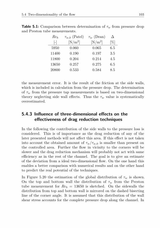
5.4 Two-dimensionality of the flow 103
Table 5.1: Comparison between determination of 𝜏𝑤 from pressure dropand Preston tube measurements.
𝑅𝑒𝑏 𝜏𝑤,𝑏 (Patel) 𝜏𝑤 (Dean) Δ[-] [N/m2] [N/m2] [%]
5950 0.060 0.065 6.511400 0.190 0.197 3.511800 0.204 0.214 4.513650 0.257 0.275 6.520800 0.533 0.584 8.5
the measurement error. It is the result of the friction at the side walls,which is included in calculation from the pressure drop. The determinationof 𝜏𝑤 from the pressure tap measurements is based on two-dimensionaltheory neglecting side wall effects. Thus the 𝜏𝑤 value is systematicallyoverestimated.
5.4.3 Influence of three-dimensional effects on theeffectiveness of drag reduction techniques
In the following the contribution of the side walls to the pressure loss isconsidered. This is of importance as the drag reduction of any of thelater presented methods will not affect this area. If this effect is not takeninto account the obtained amount of 𝜏𝑤/𝜏𝑤,0 is smaller than present onthe controlled area. Further the flow in vicinity to the corners will beslower and the drag reduction mechanism will probably not act with sameefficiency as in the rest of the channel. The goal is to give an estimateof the deviation from a ideal two-dimensional flow. On the one hand thisenables a better comparison with numerical results and on the other handto predict the real potential of the techniques.
In Figure 5.20 the estimation of the global distribution of 𝜏𝑤 is shown.On the top and bottom wall the distribution of 𝜏𝑤 from the Prestontube measurement for 𝑅𝑒𝑏 = 13650 is sketched. On the sidewalls thedistribution from top and bottom wall is mirrored on the dashed bisectingline of the corner angle. It is assumed that this distribution of the wallshear stress accounts for the complete pressure drop along the channel. In

104 5 Reference measurement
W
H
tw
1
2 3
Figure 5.20: Distribution of the skin friction on the surface of the tunnel.Top and bottom wall from measurement, side walls estimated.
the following the assumptions to calculate the decrease of effectiveness ofthe flow control techniques due to three-dimensional effects are discussed(see also illustration in Fig. 5.20).
1. The sidewalls, where no drag reduction mechanism is applicable, cover8% of surface. The maximum value of the wall shear stress on thesidewall is 80% of the mean value 𝜏𝑤,𝑏 and reduces to zero at thecorners. Therefore the integral value for the sidewalls is half of 𝜏𝑤,𝑏.This accounts for 4% of the total friction. Note that the integral valueof 𝜏𝑤 obtained from the pressure tap measurement, which is basedon two-dimensional theory neglecting any side wall effects, exceedsthe mean value of the Preston tube measurement in the same orderof magnitude (compare Table 5.1).
2. It is assumed that any technique does not influence the flow in directvicinity to corner region of covering plates (compare Fig. 5.20 surfacearea 2). In a distance to the side walls smaller than 5mm, 𝜏𝑤,𝑏 is verysmall. The average value less than 40% of 𝜏𝑤,𝑏. On the one handthe influence of any technique will be nearby zero, on the hand thisregion covers only 3% of the channel surface. The amount is 1.3% ofthe total skin friction.
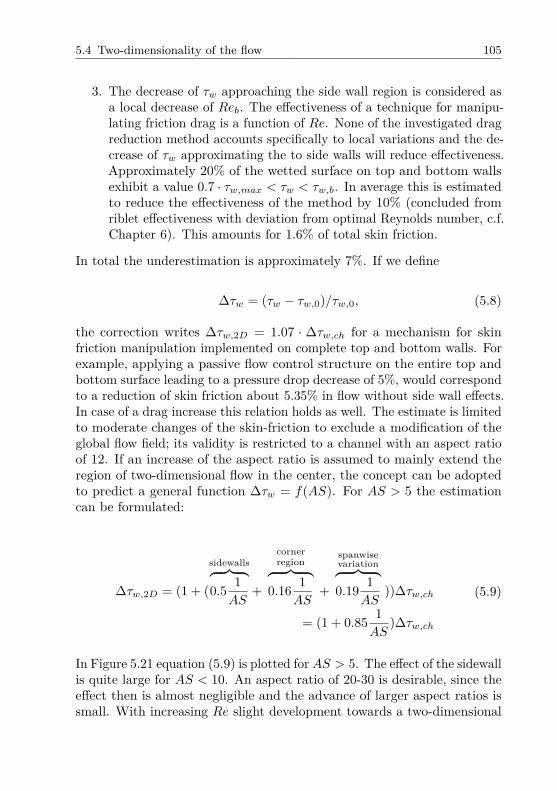
5.4 Two-dimensionality of the flow 105
3. The decrease of 𝜏𝑤 approaching the side wall region is considered asa local decrease of 𝑅𝑒𝑏. The effectiveness of a technique for manipu-lating friction drag is a function of 𝑅𝑒. None of the investigated dragreduction method accounts specifically to local variations and the de-crease of 𝜏𝑤 approximating the to side walls will reduce effectiveness.Approximately 20% of the wetted surface on top and bottom wallsexhibit a value 0.7 · 𝜏𝑤,𝑚𝑎𝑥 < 𝜏𝑤 < 𝜏𝑤,𝑏. In average this is estimatedto reduce the effectiveness of the method by 10% (concluded fromriblet effectiveness with deviation from optimal Reynolds number, c.f.Chapter 6). This amounts for 1.6% of total skin friction.
In total the underestimation is approximately 7%. If we define
Δ𝜏𝑤 = (𝜏𝑤 − 𝜏𝑤,0)/𝜏𝑤,0, (5.8)
the correction writes Δ𝜏𝑤,2𝐷 = 1.07 · Δ𝜏𝑤,𝑐ℎ for a mechanism for skinfriction manipulation implemented on complete top and bottom walls. Forexample, applying a passive flow control structure on the entire top andbottom surface leading to a pressure drop decrease of 5%, would correspondto a reduction of skin friction about 5.35% in flow without side wall effects.In case of a drag increase this relation holds as well. The estimate is limitedto moderate changes of the skin-friction to exclude a modification of theglobal flow field; its validity is restricted to a channel with an aspect ratioof 12. If an increase of the aspect ratio is assumed to mainly extend theregion of two-dimensional flow in the center, the concept can be adoptedto predict a general function Δ𝜏𝑤 = 𝑓(𝐴𝑆). For 𝐴𝑆 > 5 the estimationcan be formulated:
Δ𝜏𝑤,2𝐷 = (1 + (
sidewalls⏞ ⏟ 0.5 1
𝐴𝑆+
cornerregion⏞ ⏟
0.16 1𝐴𝑆
+
spanwisevariation⏞ ⏟ 0.19 1
𝐴𝑆))Δ𝜏𝑤,𝑐ℎ
= (1 + 0.85 1𝐴𝑆
)Δ𝜏𝑤,𝑐ℎ
(5.9)
In Figure 5.21 equation (5.9) is plotted for 𝐴𝑆 > 5. The effect of the sidewallis quite large for 𝐴𝑆 < 10. An aspect ratio of 20-30 is desirable, since theeffect then is almost negligible and the advance of larger aspect ratios issmall. With increasing 𝑅𝑒 slight development towards a two-dimensional

106 5 Reference measurement
velocity distribution is indicated by the results for the distribution ofspanwise centerline velocity and wall friction. Thus for much higher 𝑅𝑒than in the present study the change in the distribution of 𝜏𝑤 might betoo large to assume adaptability of the approach.
0 20 40 60 80 1001
1.05
1.1
1.15
1.2
AS
∆τw,2D/∆
τw,ch
Figure 5.21: Estimated influence of a channel experiment onΔ𝜏𝑤,2𝐷/Δ𝜏𝑤,𝑐ℎ in dependence of 𝐴𝑆.
The underestimation of the change in 𝜏𝑤/𝜏𝑤,0 is not the only difference toan ideal two-dimensional flow field. On the main portion of the top andbottom walls, where a drag reduction application works most effectively, thedisplacement of fluid from side walls to the tunnel center leads to an highereffective Reynolds number than 𝑅𝑒𝑏 indicates. The latter is calculated asthe integral value for the entire cross section for the experimental study.Therefore 𝑅𝑒𝑏 does not represent exactly the same quantity as for anideal two-dimensional flow corresponding to the bulk value in numericalsimulations. As a result, the higher effective bulk Reynolds number 𝑅𝑒𝑏,𝑒𝑓𝑓
of the experimental study slightly shifts the results of 𝜏𝑤/𝜏𝑤,0 to lower 𝑅𝑒𝑏.The magnitude of the shift in 𝑅𝑒𝑏 can estimated from comparison of thenumerical data with the Pitot tube measurement, which contrary to thePreston tube results is very accurate (𝛿𝑈 ≪ 1%). The spanwise centerlinevelocity is assumed to indicate the local 𝑅𝑒𝑏 for a vertical plane of thechannel, since the distribution of 𝜏𝑤 is very similar to that on the spanwisecenterline velocity. From a comparison of the velocity at the centerline ofthe DNS 𝑈𝑐,𝐷𝑁𝑆 with the Pitot tube measurement in the channel center𝑈𝑐, an increase of ≈ 2% is obtained in the experiment. If only the region

5.4 Two-dimensionality of the flow 107
70% around center of the spanwise distribution are considered, the meanvalue is ≈ 1% higher. The resulting shift in 𝑅𝑒𝑏 will be very small.
Generally, for 𝐴𝑆 = 12 the shift in 𝑅𝑒𝑏 as well as the amount of underesti-mating Δ𝜏𝑤 is smaller than the measurement accuracy commonly achievedin previous experimental or numerical investigations.
5.4.4 Summary of the reference measurements
Since this Chapter included a number of different aspects, the essentialfindings are summarized here because of their fundamental importance:
∙ For naturally developing flow, the transition occurs above 𝑅𝑒𝑡𝑟𝑎𝑛𝑠 =6000; a fully developed turbulent state on the downstream section isnot found until 𝑅𝑒 > 12000.
∙ With the artificially triggered transition a tripping level of 13% isfound to be appropriate. A fully turbulent flow was indicated for𝑅𝑒 > 5000 on both downstream sections and for 𝑅𝑒 > 4000 on thefinal section.
∙ A development length of 𝐿𝐸,𝑡𝑢𝑟𝑏 = 70 − 80𝐻 is needed for theturbulent flow. This means, on the first half of the channel length afully turbulent, but not a fully developed turbulent flow state can beachieved.
∙ For both flow states a hydraulically smooth surface is confirmed forthe entire range of 𝑅𝑒𝑏.
∙ The data scatter is small for large range of 𝑅𝑒𝑏 and generally in goodagreement to maximum scatter predicted in Chapter 4.
∙ The influence of the deviation of the wall shear stress distributionfrom an ideal, two-dimensional flow field Δ𝜏𝑤,/Δ𝜏𝑤,0 is approximately7% for the channel of the present investigation with 𝐴𝑆 = 12. Acorrection function to compute the difference has been derived.


6 Riblets
In this chapter, the previously described wind tunnel facility is used toinvestigate the effect of riblets on the flow. This investigation has two goals:The first goal is to demonstrate the flow control capabilities of the newfacility. The high quality data obtained with riblet-structured channel wallsenables comparison of the passive flow control results with the existingliterature.
The second goal is to study the streamwise flow development in a verylong channel section with riblet surfaces, which was not possible in otherinvestigations before with such high accuracy. Additionally, the limita-tions in comparability of the present results with the available literatureare discussed and the implications on the drag reduction prediction arehighlighted.
6.1 Introduction
500µm
Figure 6.1: Riblets for technical applications produced by 3M (left) (Uni-versity of Minnesota, www.safl.umn.edu) and structure of shark skin (right)(www.maritimejournal.com).
The term riblets refers to flow-aligned fins on the surface enabling a reduc-tion of skin friction up to 10% (Bechert et al., 1997). Figure 6.1 exemplary
110 6 Riblets
shows highly magnified pictures of the small scale fins on a technical fabri-cated structure and shark skin, which is a well known naturally occuringexample for riblets.The success of riblets, in contrast to almost all other ideas for reducingskin friction drag, is the achieved breakthrough in technical applications.For instance riblets are used to enhance the performance of swimmingsuits. In the recent years the application on the hull of sail boats especiallyfor the famous yacht races lead to a renaissance of the attention to thestructures. The structures have been tested on water and wind turbines(Sareen et al., 2011). Futhermore, a potential to reduce skin friction onhigh Reynolds number flows was demonstrated in test on jet airplanes andaircraft (McLean et al., 1987; Viswanath, 2002; Walsh & Sellers, 1988). De-spite their effectiveness, economic considerations showed that the requiredeffort for the application and maintenance of the structures is not cost-effective. Thus, optimization is still necessary for a profitable applicationon civil aircraft.
Walsh (1990) describes two fundamental approaches that led approximatelysimultaneously to the design of the structure. On the one hand therehave been several scientific approaches to influence near wall vortices in aturbulent boundary layer resulting in a surface with streamwise orientatedfins (Walsh & Weinstein, 1978), (Kennedy et al., 1973). On the other handthe observation of the morphology of shark skin showed small fins that arearranged in flow direction (Reif, 1978), (Reif & Dinkelacker, 1982). Thefunction of these little fins is attributed to the same mechanism of skinfriction reduction as the similar shaped technical surface.
6.2 Physical principle
The drag reduction mechanism of riblets is based on a hampering ofthe interaction of vortex structures in a turbulent flow close to the wall.Although the complexity of the process is not yet understood in all details,the development of the flow on a riblet surface can be characterized. Adetailed summary of the actual state of science is provided by Dean &Bhushan (2010). The following explanation outlines their comprehensivedescription.
The high friction drag of turbulent flows originates from an increase ofmomentum transfer in the wall normal direction, especially in the near
6.2 Physical principle 111
wall region. This transfer of momentum to the wall changes the shapeof the mean velocity profile. In consequence the velocity profile becomesfuller with a higher gradient 𝜕𝑈1/𝜕𝑥2 at the wall. Following the conceptof roughness in a turbulent boundary layer any increase of the wettedsurface enhances the shear stress. Consequently the presence of ribletstructures, which are increasing the surface, should result in an increase offriction drag. Without the usual statistical consideration of turbulence, acloser examination of the fluctuating flow reveals recurring structures inthe near-wall region. These are vortices with the axis of rotation orientatedin flow direction. The interaction of the quasi-streamwise vortices withthe surface contribute to a large extent to the momentum transfer. Theposition of the vortices is varying due to their movement in spanwisedirection. Owing to the transverse motion, adjacent vortices can collide,resulting in a fast ejection of fluid from the near wall region into the outerlayer (Kline et al., 1967). This bursting motion away from the wall, thetransverse movement of quasi-streamwise vortices and the interaction ofthese events cause additional momentum transfer and thus play a majorrole for the amount of friction drag in turbulent wall bounded flows. Onekey to reduce the friction drag is to limit these processes. One possibilityto reduce such effects is the use of specifically designed fins on the wallsurface, i.e. riblet structure. Riblets will act effectively in reducing frictiondrag, if the hampering of vortex interaction outruns the drag increase dueto the enlarged surface area.
The general mechanism is to prevent the quasi-streamwise vortices fromdirectly attaching to the wall. If the vortices only interact with the pro-truding riblet tips, the near wall region between the riblets is shielded. Incontrast to a smooth surface the vortices can not directly attach to the wall.The cross-fluctuation in between the fins of the riblets decrease, resultingin a successive lower shear stress. Although friction increases in vicinity ofthe tips the average skin friction is reduced.
The effectiveness of riblet drag reduction depends on the scaling of the struc-ture, which needs to correlate with the dimensions of thequasi-streamwise vortices. Kline et al. (1967),Walsh (1982, 1990) (ex-perimental) and Choi et al. (1993) (numerical) indicate vortex diameters inthe range of 35 to 50 wall units. As the dimensions of the vortices dependon the Reynolds number, the riblet spacing 𝑠 can only be optimized forone selected design point. For large 𝑠 the vortices come close to the wallin between the fins and interact with the increased surface area with theoutcome of higher drag than smooth surface. The visualization of vortex

112 6 Riblets
structures in a wind tunnel experiment by Lee & Lee (2001) (Fig. 6.2)shows a comparison of the behavior of streamwise vortices on a structuredwall for different Reynolds numbers. The interaction of the streamwisevortices and the surface is depicted for a riblet spacing 𝑠+ = 𝑠/𝛿𝜈 = 25and for a scaling of 𝑠+ = 40 for semi-circular riblets as used by Walsh(1983). The dimensionless spacing 𝑠+ is obtained by normalizing 𝑠 withthe viscous length 𝛿𝜈 , which is Re dependent (see Chap. 2.1.2). In the caseof drag reduction the riblets limit the spanwise movement of the vorticesand induce secondary vortices (Lee & Lee, 2001). In turn a smaller levelof the velocity fluctuations was detected. For the drag increasing case atthe higher Reynolds number, the spacing is larger than the diameter ofthe quasi-streamwise vortices. The vortices are observed closer to the walland mostly stay in between the riblet tips. Lee & Lee (2001) explain theincrease of friction drag with the down wash of high speed flow from theouter layer to the larger wetted surface of the riblet structure (Lee & Lee,2001).
Figure 6.2: Flow visualization of streamwise vortices on a plate with circularriblets at 3m/s (drag decreasing) and 5m/s (drag increasing) from Lee &Lee (2001). Reproduced with kind permission from Springer Science andBusiness Media.
To quantify the relation between the riblets geometry and the amountof skin friction reduction Bechert & Bartenwerfer (1989) introduced theconcept of protrusion height difference. The protrusion height is definedas the difference of vertical shift of the flow origin to the tip height of theriblets (Fig. 6.3). This parameter can be calculated for the flow parallelℎ𝑝𝑠 and in cross direction ℎ𝑝𝑐 to the fins. The difference of the two flow

6.2 Physical principle 113
Figure 6.3: Concept of protrusion height difference taken from Bechertet al. (1997). Reproduced with permission.
s
s1
Luchini et al. (1991)
roughnesselement
riblets withinviscoussublayer
t
t
ww0
opt
+DB
linea
rla
w
log law
logx2
U+ 1
U+ 1
-DB
linea
rla
wlog law
logx2
+
+
Figure 6.4: Schematic illustration of the effect of riblets on skin frictionincluding the theoretical estimation by Luchini et al. (1991) for small 𝑠.
origins is named the protrusion height difference 𝛿ℎ. The protrusion heightdifference is an extent to the riblet’s capability of hampering the transversemotion of the quasi-streamwise vortices. Since this concept is based onviscous theory, it is only valid if the riblets are embedded in the viscoussublayer. With increasing 𝑠+ the riblets grow out of the sublayer andthe concept of protrusion height difference loses its validity. Theoreticalconsiderations by Luchini et al. (1991) support the concept of protrusionheight. In oil tunnel experiments Gruneberger & Hage (2011) examinedthe effect of small riblet spacings and found the effect of the riblets linearlydecreasing with the riblet spacing for 𝑠 < 𝑠𝑜𝑝𝑡, which is in accordance toBechert’s and Lucchini’s theories (compare Fig. 6.4).

114 6 Riblets
There is a number of experimental and numerical studies consideringthe drag reduction mechanism of riblets from differing points of view.Exemplarily Lee & Choi (2008) pay attention to the presence of spanwisevortices in their PIV experiments. Spanwise vortices are in close relationto the mechanism of sweeps and ejections. Their finding is a modificationof the spanwise vortices in the near wall region. Especially the number ofvortices with a rotation in counter direction to the near wall flow, which areresponsible for the drag increasing ejection event, is significantly reduced.In numerical investigation Choi et al. (1993); Garcia-Mayoral & Jimenez(2011) were able to analyze the flow field surrounding the riblets and toidentify vortex structures in the vicinity of the riblet tips.
The mentioned observations from varying points of view consider differentaspects and show different mechanisms of the riblets effecting the flow.These are not in contradiction, but contribute to an overall picture, viewedfrom differing angles. Today’s discussion on the mechanisms is the question,which are the underlying mechanisms and which are an implication ofthose.
Regarding the riblet’s impact on a turbulent boundary, three main parame-ters have been identified: The spanwise distance between the fin tips, whichis named the riblet spacing 𝑠, the total riblet height ℎ from the lowestpoint in valley between the fins to the tips and the riblet shape. 𝑠 and ℎcan be transformed to nondimensional quantities as introduced in Chapter2.1.2:
𝑠+ = 𝑠
𝛿𝑣, ℎ+ = ℎ
𝛿𝑣(6.1)
For the optimum geometric parameters Bechert et al. (1997) give a spacingof 𝑠+ = 16 to 𝑠+ = 17 and ratio ℎ/𝑠 = 0.5, which is in general agreementto other literature (Dean & Bhushan, 2010; Walsh, 1990). One shoulddenote that this specification varies for different geometries since oftenboth critera cannot be kept simultaneously. In the case of sawtooth shapethe ratio is a function of the tip angle 𝛼. For the extensively studiedgeometry with 𝛼 = 60∘, which has been produced industrially by 3M,the ratio is ℎ/𝑠 = 0.87. It can be summarized that for optimum effec-tiveness the riblet tips slightly reach into the buffer layer ℎ+ > 5, butare still far from the logarithmic layer. The optimum rib spacing is ap-proximately half the diameter of a quasi-streamwise vortex. Schematicallythe dependence of 𝜏𝑤/𝜏𝑤,0 on the riblet spacing is summarized in Figure 6.4.

6.2 Physical principle 115
The optimal design for riblets is an arrangement of infinitely thin verticalblades. This geometry was realized in good approximation by Bechert et al.(1997) and led to the highest skin friction reduction of 9.9% verified inexperiments so far. Luchini’s analytical considerations confirmed the bladeshape as the most effective (Luchini, 1993). Although the blade ribletsshowed highest effectiveness, their practical use is restricted due to theirvulnerability to mechanical loads. Walsh (1990) suggested to further studytriangular riblets with a flat interspace. (Bechert et al., 1997) reporteda decrease of 8% in skin for such a configuration, which is quite close tothe blade riblets. This shape appears to be a good compromise betweendurability and performance. Further investigations with this geometry wereconducted by Gruneberger & Hage (2011).
During the last 20 years the attempt was made to improve riblets effective-ness by modeling the shape in streamwise direction. Length, arrangementand flexibility of the structures were varied to simulate natural shark skin(Bechert et al., 1997). Additional effort was put on the modification of ri-blets to a wave like structure to induce a supplemental spanwise mechanism(Gruneberger & Hage, 2011). In experimental investigations these modifi-cations did not show benefits compared with the standard two-dimensionalgeometry of riblets. In contrast the drag reduction was even less.
The effectiveness of riblets could be verified up to the region of transonicflows (Viswanath, 2002; Walsh, 1990), where a slight increase of the perfor-mance was indicated. In addition, riblets have also been tested in laminarand transitional flow. In the first case some few investigations report smalldrag reduction (Fulachier et al., 1987; Liandrat, 1988). In studies at theLangley Research Center no changes of the skin friction could be found(Walsh, 1990), which is in accordance to theoretical study of Choi et al.(1991). Thus Walsh (1990) condiders the drag reduction reported in afore-mentioned studies to be related to uncertainty of the detection procedere.Today it is common sense that riblets only reduce drag in turbulent flows.In laminar flow the complete mechanism described for turbulence is noteffective due to the absence of quasi-streamwise vortices. The structureswill act as roughness elements and increase the wetted surface.
In transitional flow, sources in literature are not in complete agreement,but a transition delay has not been definitely proofed. For instance astudy on an airfoil on glider plane conducted by Quast is reported in

116 6 Riblets
Bechert (1988), where initially promising reduction of skin friction changeis stated to be related to the control of a separation bubble. In thetheoretical work of Lucchini (1995) a modification of the instabilities intransition could be found, but a clear statement, whether this would leadto a significant reduction of friction drag was not made. Hence, the presentstudy concentrates on 2D-shaped riblets in turbulent flow conditions.
6.3 Experimental study of riblets
6.3.1 Experimental investigation - State-of-the-art
Within the large number of articles on this topic two outstanding sources ofcomprehensive experimental work are found: The investigations of Walshand the studies of Bechert. In the early 1980s Walsh’s pioneering workyielded a comprehensive characterization of the effect of riblets (Walsh, 1982,1983; Walsh & Lindemann, 1984). Within a short period many differentgeometries have been examined. Bechert’s investigations are outstandingespecially because of the high accuracy measurements (Bechert et al., 1992).Both authors extensively studied the effect of the riblet geometry on dragreduction. A summary of those results is given in Bechert et al. (1997) andWalsh (1982) respectively Walsh & Lindemann (1984) .
Walsh (1983) calculated the height of the riblets for cruise flight (𝑀𝑎 = 0.8)at an altitude of 12.2 km and a Reynolds number 𝑅𝑒𝑥 = 106 as ℎ =0.076mm. Difficulties of riblet fabrication and the influence of apparentimperfections originating from manufacturing processes result in significantexperimental uncertainty, as shown by Walsh & Lindemann (1984). ThusWalsh points out the challenge which still concerns a lot of engineers andscientist: The application and high quality fabrication of the small scalestructures on large surface area.
In laboratory experiments the difficulty of fabrication can be reduced, usingliquids as flow medium. Bechert et al. (1992) utilize the favorable ratio ofdynamic viscosity to density of oil compared to air (𝑣𝑜𝑖𝑙 = 1.20×10⁻⁵𝑚2/𝑠).The riblet size at equivalent Reynolds number grows from few tenths of amillimeter in air to few millimeters in oil.
For the purpose of riblet testing a new oil tunnel facility was designed andbuilt in Berlin (Bechert et al., 1992), possessing very high measurement

6.3 Experimental study of riblets 117
s
ha
Figure 6.5: Schematic sketch of riblets type with trapezodial geometry.
accuracy. While Walsh specifies a value of ±1% accurary for the determi-nation of friction change in his wind tunnel facility, which partly seemsoptimistic regarding the presented results, Bechert attains ±0.3%.
It has to be denoted that oil and water tunnels have a disadvantage. Ifthe streamwise length of the riblet surface is considered as a multipleof the riblet height, wind tunnels can be equipped with a much longerriblet surfaces, which is necessary to study the flow development on thestructures.
6.3.2 Design and fabrication of the structures
Since at the time of the present study riblet surfaces have not been availableon the market, it became inevitable to manufacture the structures. Toobtain a preferably high amount of difference in friction between the smoothreference and the riblet surface, a triangular geometry with flat interspaceswas chosen (Fig. 6.5). This design promises the optimum compromisebetween manufacturing capabilities and a high reduction of skin friction(Gruneberger & Hage, 2011). The calculation of the geometric parametersis carried out following Bechert et al. (1997), who extensively studiedthis riblet shape. With decreasing tip angles (60∘, 45∘, 30∘) an increase ineffectiveness was found. Accordingly a geometry with a ratio ℎ/𝑠 = 0.5,𝑠+
𝑜𝑝𝑡 = 16.5 and the sharpest contrivable tip angle was selected (53.5∘) forthe present study. The design Reynolds number was chosen to 𝑅𝑒𝑏 = 11700in order to guaranty fully turbulent flow, even in a wide range below theoptimum (𝑠+ < 𝑠+
𝑜𝑝𝑡). Due to the agreement of the results in Chapter5.2 with Dean’s formula, the calculation of 𝜏𝑤 is based on this empiricalcorrelation for the riblet design. Table 6.1 presents the caculated geometryfor the selected design point.

118 6 Riblets
The structures were manufactured in a large milling machine at the Fraun-hofer Institute for Production Technology of the RWTH Aachen. Specialdiamond cutting tools were custom made by Mossner in Pforzheim. Thedimensions of the tools slightly deviate from the design values which led tominimal differences of the geometry (Tab. 6.1). Two plates with a struc-tured surface area of 1500mm x 300mm were produced with micrometerprecision. A cross section view of the riblets is presented in Figure 6.6.
Planarity is guaranteed by the use of 15mm aluminium baseplates. A thicklayer of plastic material is screwed on the baseplates and the surface hasbeen milled to planarity before in the final step the riblet structure wasfabricated. Due to machinability and minor abrasion of the tool it hasbeen decided to use plastic material for the riblets. Indeed a single cuttingtool did the job and thus ensured the structure to be identical over theentire surface. Especially the crucial tips of the riblets could be realized inan excellent finish.
From the viewpoint of a channel experiment also the intersection betweenthe smooth plates and riblet plates needed to be considered. Accordingto Bechert et al. (1997) an abrupt begin of the riblet surface should notalter the flow at the onset of the riblet plate. However, due to the smalldimensions of the present channel a change of the cross sectionial areadue to the presence riblets is not negligible. Therefore the cross sectionarea is kept constant by increasing the channel height to compensate forthe blockage arising from the protruding riblets. This was realized by aprotruding frame on both sides of the riblet plate. In Figure 6.7 the stepof 70𝜇m at the contact surface of the side wall is shown.
70µ
m
53.5°
614µm
294µ
m
Figure 6.6: Cross sectional view on trapezodial riblets manufactured atRWTH Aachen.

6.3 Experimental study of riblets 119
smooth plate
side wall
riblet plate
Figure 6.7: Detail of the intersection between the riblet, the smooth plateand the side wall. The direction of view is upstream.
Table 6.1: Designed and resulting dimensions the produced riblets𝑠 [𝜇m] ℎ [𝜇m] tip angle [∘] 𝑅𝑒𝑜𝑝𝑡
Design 600 300 53.5 11700Result 614 294 53.5 11400
6.3.3 Focus of the experimental investigations
Besides the necessity to demonstrate the effectiveness of the passive drag re-duction mechanism in the developed facility with an high accuracy measure-ment system, there remain some contraverse discussed aspects concerningthe flow development on riblet surfaces, on which the present experimentallysetup might be able to shed some light. Therefore, the following paragraphdepicts differences between the present set-up and the measurement tech-nique from Walsh (1982) and Bechert et al. (1992). Considering a largenumber of literature data from different authors Walsh (1990) found thosemeasured with a shear stress balances to be most accurate and reliable.Hence, Bechert as well as Walsh use shear stress balances in their studies.One disadvantage is that shear stress balances only provide integral dragvalues of the test plate. The streamwise development of 𝜏𝑤 is not resolved.Walsh (1982) investigates the effect of flow development by covering partlyhis test plate with tape to generate a smooth surface. The result shows aproportional relation between the riblet area and 𝜏𝑤/𝜏𝑤,0. However, theaccuracy of this procedure is questionable and a fine resolution cannotbe achieved. The measurement of the pressure difference 𝑑𝑝/𝑑𝑥 in thepresent study automatically resolves the development in the flow directiondepending on the number of pressure taps along the test plate.

120 6 Riblets
Of particular interest is the question whether there is a streamwise distancerequired for reduction of skin friction and how long it is. Walsh collectedsome data concerning the flow development over a riblets surface and foundinconsistent results (Walsh, 1990). While his own measurement indicatedhigher local skin-friction reduction, Gallagher & Thomas (1984) foundthe skin friction reduction to be less at the leading region of the riblets.Savill (1986) finds an immediate response to the presence of the structures,indicating a negligible development length. One difficulty is the adjustmentof the begin of the riblets. On the one hand in Squire & Savill (1986, 1987)the leading edge affects the results. On the other hand Bechert et al. (1997)found no leading edge effect even for an abrupt begin of the riblet.
6.3.4 Arrangement of experimental setup
For the riblet investigation the channel is equipped with the 13%-trippingat 𝑥 = 0 to trigger a turbulent flow. The structures are located in thedownstream part of the test section 𝑥 > 98𝐻, where a fully developedturbulent flow is observed in the reference measurement (cf. Chap. 5.2).Experiments were conducted for a range of 𝑅𝑒𝑏 = 3700 − 23500. For thiswide range two different flow rate instrument have been used: The orificemeter with the 60mm disk and the inlet nozzle with 𝐷 = 74mm. Duringthe measurement the pressure distribution over the total length of thetest section has been read, but the data presented omit the first section,which is mainly affected by flow development on the 1000mm from thebegin of the channel section. Results are presented starting at the sixthpressure tap located at 40H. The last pressure tap with a distance of 50mmto the end of the channel is also not shown, since the tap was obviouslyaffected by the outlet for high Reynolds numbers (cf. Chap. 5.2). Thus theobserved length is 1400mm on smooth surface, followed by the intersectionof 100mm (50mm smooth, 50mm riblets) and a riblet length of 1200mm.In the following these sections are denoted “upstream” and “downstream”.Both Baratron differential pressure sensors were used in combination withthe Scanivalve multiplexer, where the first and the central tap have beenread simultaneously by both sensors to check alignment of the sensors. Theresults are averaged over 180s for each pressure tap, resulting in 36min intotal for one test series including 20 (22) readings.

6.4 Discussion of the results 121
6.4 Discussion of the results
To obtain an idea of the quality of the data and to present the effectof the riblets qualitatively, Figure 6.8 presents the friction coefficient independence of 𝑅𝑒𝑏 for the fully turbulent developed flow on downstreampart of the test section for both surface conditions. Obviously the ribletsare effective, since the 𝑐𝑓 is lower for the structured surface at small andmoderate 𝑅𝑒𝑏. With increasing 𝑅𝑒𝑏 the distance between the two curvesdiminishes until finally the riblets act as additional roughness increasingthe 𝑐𝑓 . This observation is in agreement with the expected result.
5000 10000 15000 200005
6
7
8
9
10x 10
−3
Reb
cf
ReferenceRiblet
Figure 6.8: Comparison of friction factor 𝑐𝑓 for smooth and structuredsurface in the downstream part of the test section. Open symbols indicatemeasurement with the orifice meter, filled symbols with inlet nozzle.
For further analysis we will first take a look at the distribution of thepressure loss (Fig. 6.10 and 6.11) in streamwise direction, shown pairwisefor correlating 𝑅𝑒𝑏. In the upstream section the surface is always smooth,while in the downstream part the surface consition is either smooth (right)and structured surface (left). Exemplarily a detailed look is provided inFigure 6.9 for 𝑅𝑒𝑏 = 11300. Scatter in the data is very low for both surface

122 6 Riblets
1 1.5 2 2.5 3 3.5 40
10
20
30
40
50
60
x [m]
∆pl[Pa]
Reb =1130015.63 Pa/m14.42 Pa/m
Figure 6.9: Pressure drop over smooth (+) and structured (x) surface alongthe channel.
conditions. The two lines show least-square-fits, one drawn through theeight taps of the smooth plate (Δ𝐿 = 1400mm) and the other (dashed line)through the seven taps of the riblet plate (Δ𝐿 = 1200mm). From figuresFigures 6.10 and 6.11 a linear dependance of the static pressure gradienton the downstream position can be obtained. The residua 𝑅 for the linearfit over seven considered pressure taps are 𝑅 > 0.99996 for any of 120 datasets with riblet surface (and for the smooth surface as well). Neither anincrease nor a decrease in riblets performance with respect to 𝑥 can befound. Any development induced at the leading edge of the riblet plate isdefinitely vanished at 50mm which is equivalent to 2𝐻 or approximately67ℎ+. This observation is similar for all 𝑅𝑒𝑏. For the lower 𝑅𝑒𝑏 withsmaller pressure drop on the riblet surface than on the smooth plate as wellas for 𝑅𝑒𝑏=22230, where the 𝑑𝑝/𝑑𝑥 is larger on the riblet surface Walsh’sproportional relation is confirmed. Surprisingly, the intersection betweenthe smooth and the riblet surface, which is not taken into account for thecalculation of 𝜏𝑤/𝜏𝑤,0, exhibits a remarkable detail. The pressure taps nextto the intersection, which were set in a closer distance of 100𝑚𝑚 to eachother, consisting of 50mm smooth and 50mm structured surface. Despite

6.4 Discussion of the results 123
1 1.5 2 2.5 3 3.5 40
10
20
30
40
x [m]
∆pl[Pa]
Reb =879010.11 Pa/m9.42 Pa/m
(a) 𝑅𝑒𝑏 = 8790
1 1.5 2 2.5 3 3.5 40
10
20
30
40
x [m]
∆pl[Pa]
Reb =887010.48 Pa/m10.31 Pa/m
(b) 𝑅𝑒𝑏 = 8870
1 1.5 2 2.5 3 3.5 40
10
20
30
40
50
60
x [m]
∆pl[Pa]
Reb =1150016.17 Pa/m14.95 Pa/m
(c) 𝑅𝑒𝑏 = 11500
1 1.5 2 2.5 3 3.5 40
10
20
30
40
50
60
x [m]
∆p l
[Pa]
Reb =1150016.48 Pa/m16.24 Pa/m
(d) 𝑅𝑒𝑏 = 11500
1 1.5 2 2.5 3 3.5 40
20
40
60
80
x [m]
∆p l
[Pa]
Reb =1515026.10 Pa/m24.46 Pa/m
(e) 𝑅𝑒𝑏 = 15150
1 1.5 2 2.5 3 3.5 40
20
40
60
80
100
x [m]
∆pl[Pa]
Reb =1511026.87 Pa/m26.43 Pa/m
(f) 𝑅𝑒𝑏 = 15110
Figure 6.10: Comparison of pressure drop for completely smooth testsection (right) and with the downstream section equipped with riblets (left)for different 𝑅𝑒𝑏.

124 6 Riblets
1 1.5 2 2.5 3 3.5 40
20
40
60
80
100
120
x [m]
∆p l
[Pa]
Reb =1795034.96 Pa/m33.58 Pa/m
(a) 𝑅𝑒𝑏 = 17950
1 1.5 2 2.5 3 3.5 40
20
40
60
80
100
120
x [m]
∆pl[Pa]
Reb =1809036.25 Pa/m35.73 Pa/m
(b) 𝑅𝑒𝑏 = 18090
1 1.5 2 2.5 3 3.5 40
50
100
150
x [m]
∆p l
[Pa]
Reb =2223051.36 Pa/m52.20 Pa/m
(c) 𝑅𝑒𝑏 = 22230
1 1.5 2 2.5 3 3.5 40
50
100
150
200
x [m]
∆p l
[Pa]
Reb =2239054.32 Pa/m53.39 Pa/m
(d) 𝑅𝑒𝑏 = 22390
Figure 6.11: Comparison of pressure drop for the completely smooth testsection (right) and the downstream section equipped with riblets (left) fordifferent 𝑅𝑒𝑏.

6.4 Discussion of the results 125
of the pressure loss of the average value of smooth and riblet surface, thedata show a higher 𝑑𝑝/𝑑𝑥 than for the smooth plate. Since the referencedata for the completely smooth channel (right column of Fig. 6.10 and6.11) do not indicate any variation in 𝑑𝑝/𝑑𝑥 at the intersection, the effectmust be related to the begin of the riblet plate. Obviously this observationis in contradiction to Bechert et al. (1997), who stated that an abruptintersection between smooth the surface and riblets would not affect theresults. Walsh (1982) reports a study by Sawyer & Winter (1987), wheretwo configurations of the experimental set-up with a drag balance have beentested. In the first configuration the riblet structures were only located onthe plate of the balance. In the second configuration the walls of the windtunnel surrounding the drag balance were also with equipped with riblets.They reported no effect on the measurement results. Both authors couldnot resolve the development at the intersection, but refer to an integral dragvalue of the riblet surface, which may be affected slightly from the leadingedge. This is considered to be the cause for the disagreement to the presentexamination. It needs to be mentioned here that nevertheless Bechert usedoptimized intersections for his measurement to exclude possible influenceof the intersection. Details on this procedure are shown in appendix ofBechert et al. (1997).
In the present facility the pressure drop reacts quite sensitive even tosmall variations of the channel height 𝐻. At the intersection the effectof a backward facing step to keep the cross section constant cannot bedistinguished from the influence of the protruding riblets. Note that thestep is only 70𝜇m on bottom and top wall, which in sum is far less than 1%of 𝐻. This indicates, that there is substantial contribution of the 225𝜇mprotruding riblets. In wind tunnels of conventional dimensions such asmall step influences only insignificantly the mean velocity and thus 𝑅𝑒𝑏.Therefore, this is not critical for the result of the shear stress 𝜏𝑤. Thediffering reports in the literature might be influenced more by the detailsof the setup than by the riblets themselves. The result of the presentstudy shows how critical small details in the design affect the results, if thequantities to be measured are small.

126 6 Riblets
6.4.1 Strategy to determine the skin friction change
The decrease in skin friction can be determined by a comparison of 𝑐𝑓,0 fora smooth and 𝑐𝑓 for a riblet surface in the rear part of the channel as itwas shown in Figure 6.8.
𝜏𝑤/𝜏𝑤,0 = 𝑐𝑓 /𝑐𝑓,0 (6.2)
The measurement uncertainty is then depending on two stochastic errors,namely the reproducibility of 𝑐𝑓 , which can be assumed to be the same inthe structured data. A Gaussian error propagation would lead to
√2 · 𝛿𝑐𝑓 ,
resulting in an uncertainty of 0.4 to 1.3% depending on 𝑅𝑒. The uncertaintyis the result of the fact that the measurement needs to be conducted twotimes and the individual uncertainties of each measurement add (compareChap. 4.3.2). The balance measurement by Bechert et al. (1997) directlycompares the smooth and the structured surface and avoids this source oferror. An additional disadvantage of the comparison of the downstreamsection data for different surface conditions is the presentation of theresults. A comparison can only be made between two curve fits of theslightly scattered data for the smooth and the structured surface (Fig. 6.8).A direct comparison of single data points can hardly be drawn. Thus wewill go a second way to calculate 𝜏𝑤/𝜏𝑤,0 avoiding the reproduction error.
A direct comparison of the smooth and the structured surface is enabled,if both surface conditions are realized in one measurement. This can beachieved by comparison of the downstream riblet section with the upstreamsmooth section. The skin friction change can be calculated:
𝑐𝑓
𝑐𝑓,0= (Δ𝑝𝑙/Δ𝐿)
(Δ𝑝𝑙,0/Δ𝐿0) . (6.3)
However, from the reference measurement we know that the flow is fullydeveloped for a channel length of 𝑥 ≥ 80H. So the flow development slightlyinfluences the smooth upstream section of the channel. In consequencethe smooth upstream section exhibits little more pressure loss and thecomparison would to lead an apparent skin friction reduction, originatingfrom incomplete flow development on the upstream section. Thus a directcomparison can only be drawn, if the degree of this “under-development”can be determined. Therefore in Figure 6.12 the ratio of the skin friction on

6.4 Discussion of the results 127
5000 10000 15000 200000.9
0.95
1
1.05
1.1
1.15
Reb
τw,ds/τ
w,us
nozzleorifice
Figure 6.12: Ratio between the skin friction on the downstream and theupstream plate for a smooth reference channel for 𝑅𝑒𝑏 = 3700 − 23000.
the upstream and the downstream section for the complete smooth channelis shown. A constant relation between the pressure loss on the two sectionsis obtained for 𝑅𝑒𝑏 > 5000 (Fig. 6.12), where the flow is fully turbulent. Ifit is possible to show, that the results from the upstream part are exactlythe same independent of whether a smooth or a structured plate is locateddownstream, a constant factor 𝑘𝑑 can be determined (Eq. 6.4), which isused to correct the result of 𝑐𝑓 /𝑐𝑓,0:
(Δ𝑝𝑙,0/Δ𝐿0)downstream
(Δ𝑝𝑙,0/Δ𝐿0)upstream= 𝑘𝑑. (6.4)
Then 𝑑𝑝/𝑑𝑥 for downstream section with riblets and the smooth upstreamsection can be directly compared:
𝑐𝑓
𝑐𝑓,0=
(Δ𝑝𝑙/Δ𝐿)(Δ𝑝𝑙,0/Δ𝐿0)
𝑘𝑑. (6.5)
The constant is determined from Figure 6.12 to 𝑘𝑑 = 1.016.
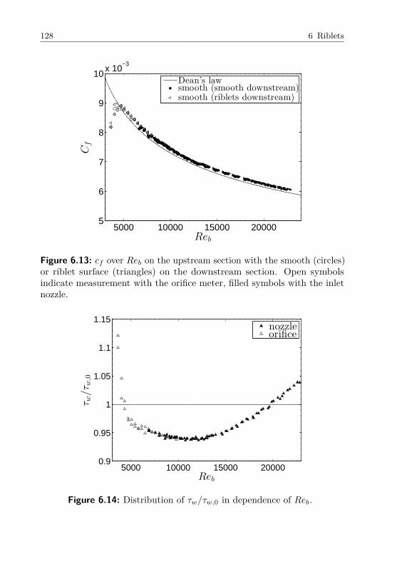
128 6 Riblets
5000 10000 15000 200005
6
7
8
9
10x 10
−3
Reb
Cf
Dean’s lawsmooth (smooth downstream)
smooth (riblets downstream)
Figure 6.13: 𝑐𝑓 over 𝑅𝑒𝑏 on the upstream section with the smooth (circles)or riblet surface (triangles) on the downstream section. Open symbolsindicate measurement with the orifice meter, filled symbols with the inletnozzle.
5000 10000 15000 200000.9
0.95
1
1.05
1.1
1.15
Reb
τw/τ
w,0
nozzleorifice
Figure 6.14: Distribution of 𝜏𝑤/𝜏𝑤,0 in dependence of 𝑅𝑒𝑏.

6.4 Discussion of the results 129
Considering the uncertainty in a distribution of 𝜏𝑤/𝜏𝑤,0 over 𝑅𝑒𝑏 thereproducibility of the flow rate measurement will be the dominating factor inrelation to the small errors originating from the pressure drop measurement.The reproducibility of the flow rate will lead to a horizontal scatter of thedata points, whereas the uncertainty originating from the pressure dropreading is very small, since it depends only on the reproducibility of thehigh accuracy sensors from MKS (see Chap. 4.3.2).
The validity of this procedure is verified by the comparison of the frictioncoefficient on the smooth downstream plate for the case of the referenceand the riblet measurements in Figure 6.13. The curve fits of each dataset demonstrate a minimum difference between both test series over thecomplete range of 𝑅𝑒𝑏. For smaller 𝑅𝑒𝑏 a slight difference of 0.2% isobtained, which is hardly visible in the diagram and lies clearly withinthe measurement accuracy. Note that the difference between the flowrate instruments in a range of 6700 < 𝑅𝑒𝑏 < 7500 is due to the lowerlimit of validity of the calibration of the nozzle (filled symbols) and is alsorepeatable for both conditions of the test section.
For the use of this strategy to determine 𝜏𝑤/𝜏𝑤,0 it is fundamental to havea fully turbulent flow at the beginning of the upstream plate, which is notthe case for small 𝑅𝑒𝑏 as can be seen in Figure 6.12. The benefit of thisstrategy with respect to the confidence of 𝜏𝑤/𝜏𝑤,0 is limited to 𝑅𝑒 > 7000,where the scatter in the data is small and there is sufficient clearance tothe transitional regime. The result of 𝜏𝑤/𝜏𝑤,0 is presented in Figure 6.14.Indeed for 𝑅𝑒𝑏 > 7000 a small scatter in the range of ±0.5% to ±0.2% isobserved, while for smaller 𝑅𝑒𝑏 the scatter is higher. At 𝑅𝑒𝑏 < 4800 theflow along the upstream plate is still transitional and the data indicate alower drag on the downstream plate due to partly laminar flow. This wasalso seen in Figure 6.12. Therefore, the following discussion will not takeinto consideration measurements for 𝑅𝑒𝑏 < 5000.
6.4.2 Change of the skin friction drag
A direct comparison of data from the study of trapezoidal riblets fromBechert et al. (1997) with the present results is given in Figure 6.15. Ingeneral, agreement with the data of Bechert et al. (1997) is found. Thegraph for the used 53.5∘-riblets lies in between the curves of 45∘ and 60∘-Riblets from Bechert’s data. The optimum spacing 𝑠+
𝑜𝑝𝑡 = 16.5 is exactlythe same and the maximum drag reduction of 6.0% represents the expected
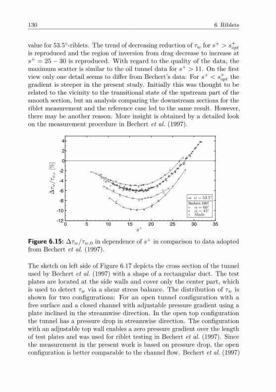
130 6 Riblets
value for 53.5∘-riblets. The trend of decreasing reduction of 𝜏𝑤 for 𝑠+ > 𝑠+𝑜𝑝𝑡
is reproduced and the region of inversion from drag decrease to increase at𝑠+ = 25 − 30 is reproduced. With regard to the quality of the data, themaximum scatter is similar to the oil tunnel data for 𝑠+ > 11. On the firstview only one detail seems to differ from Bechert’s data: For 𝑠+ < 𝑠+
𝑜𝑝𝑡 thegradient is steeper in the present study. Initially this was thought to berelated to the vicinity to the transitional state of the upstream part of thesmooth section, but an analysis comparing the downstream sections for theriblet measurement and the reference case led to the same result. However,there may be another reason. More insight is obtained by a detailed lookon the measurement procedure in Bechert et al. (1997).
Figure 6.15: Δ𝜏𝑤/𝜏𝑤,0 in dependence of 𝑠+ in comparison to data adoptedfrom Bechert et al. (1997).
The sketch on left side of Figure 6.17 depicts the cross section of the tunnelused by Bechert et al. (1997) with a shape of a rectangular duct. The testplates are located at the side walls and cover only the center part, whichis used to detect 𝜏𝑤 via a shear stress balance. The distribution of 𝜏𝑤 isshown for two configurations: For an open tunnel configuration with afree surface and a closed channel with adjustable pressure gradient using aplate inclined in the streamwise direction. In the open top configurationthe tunnel has a pressure drop in streamwise direction. The configurationwith an adjustable top wall enables a zero pressure gradient over the lengthof test plates and was used for riblet testing in Bechert et al. (1997). Sincethe measurement in the present work is based on pressure drop, the openconfiguration is better comparable to the channel flow. Bechert et al. (1997)

6.4 Discussion of the results 131
present a comparison of measurement data with both configurations, whichis shown in Figure 6.16. If the data from the open top configuration areconsidered, the gradient for 𝑠+ < 𝑠+
𝑜𝑝𝑡 appears to be similar to the data ofthe present study. It is assumed that the difference in the measurementfor small 𝑠+ is caused by the pressure gradient. However, this still cannotexplain the steeper gradient. From the theoretical point of view a linearbehavior matching the coordinate origin according to Luchini’s theory isexpected. The open tunnel configuration in the study of Bechert providessignificantly more uniform spanwise distribution of 𝜏𝑤, which should betteragree to the theory (for further details see the following section). Butthe opposite is the case. How the different spanwise distribution of 𝜏𝑤
influences the drag reduction for riblets with 𝑠+ < 𝑠+𝑜𝑝𝑡 remains open.
open channel
closed channel
Figure 6.16: Distribution of 𝜏𝑤 over Re in dependence on tunnel configu-ration redrawn from Bechert et al. (1997).
6.4.3 Influence of spanwise velocity distribution
As discussed in Section 5.4 the investigated channel flow exhibits a nearlyuniform velocity distribution in the center part of its cross section. Close tothe side walls the shear stress deviates from a two-dimensional distribution.This was examined in Chapter 5.4. The presence of the unstructured sidewalls causes additional friction. In consequence one could expect the dragreduction with the same riblet geometry to be less than in experiments inother facilities. Nevertheless, even without the correction for the flat duct(Eq. 5.9) the agreement is quite good.

132 6 Riblets
In the following some general aspects affecting the measurement are dis-cussed based on a comparison of the present set-up with the experimentalfacilities used by Walsh (1982) and Bechert et al. (1997).
In Walsh (1982, 1983) and Walsh & Lindemann (1984) a wind tunnel witha rectangular cross section of 279mm x 178mm and a length of 914mm hasbeen used. This cross section geometry with an aspect ratio of 1:1.5 doesnot provide a smooth lateral shear stress distribution. With dimensions of279mm x 178mm the test plate uses the complete lateral spacing of thetunnel including the secondary flow dominated region close to the cornerswhich significantly influence the velocity distribution.
Bechert et al. (1997) give an comprehensive description of their facility inBechert et al. (1992). In the appendix to their article, Bechert et al. (1997)also present the test section in riblet testing configuration in detail. Witha cross section of 250mm x 850mm an aspect ratio of approximately 1:3.5is achieved. The drag balance is located in the middle part of the 850mmlong side wall with a width of 400mm. Advantageously in this arrangementthe sidewall effects can be eliminated to some degree. Otherwise the aspectratio of 1:3.5 is not large enough to guarantee a two-dimensional velocitydistribution in the middle part. The lateral distribution of 𝜏𝑤 on a flatand a riblet plate was determined with a Preston tube in the oil tunnel.Figure 6.17 shows the results for open channel and zero pressure gradientconfiguration. In both cases the skin friction is higher in the middle anddecreases in lateral direction. For the zero pressure configuration, whichhas been used for the riblet tests, the profile becomes asymmetric andthe wall shear stress variation of 20% is much higher. The variation inflow direction is not shown, but it can be assumed that the deceleration ofthe fluid needed to achieve 𝑑𝑝/𝑑𝑥 = 0 will also cause a variation of shearstress in flow direction. Note that the difference in drag reduction for lowReynolds number presented in Figure 6.16 is considered to be a pure resultfrom differing tunnel configuration, meaning the 𝜏𝑤 distribution, in Bechertet al. (1997).
In summary, measurement results in all three facilities are affected by a non-constant shear stress distribution which can slightly influence the maximumamount of drag reduction. As indicated in Figure 6.16 the deviation mightbe larger for 𝑠+ < 𝑠+
𝑜𝑝𝑡 depending on the chosen experimental procedure.For a comparison of experimental with numerical 2D data these should bekept in mind.

6.4 Discussion of the results 133
(a) Open tunnel configuration
(b) Closed tunnel configuration
Figure 6.17: Cross sectional view of the test section of the Berlin oil tunneland the corresponding shear stress distribution with open tunnel (a) andfor zero pressure configuration (b) from Bechert et al. (1997). Reproducedwith permission.

134 6 Riblets
6.5 Conclusions
The investigation of riblet structures verified two important aspects. Firstthe measurements are in very good agreement with the results of Bechertet al. (1997) which has been deemed to be the most accurate experimentaldata for riblets for the time being. A very good quantitative agreementbetween the results presented in this study and Bechert et al. (1997) isfound: The optimum riblet spacing 𝑠+
𝑜𝑝𝑡 = 16−17 as well as 6% skin frictionreduction match Bechert’s data. For the present set-up the deviation froma uniform distribution of the skin friction can be recalculated exploitingequation 5.9 yielding a slightly higher drag reduction of 6.4%.
Second, the scatter of the data lies within the calculated uncertainty,supporting the careful and detailed uncertainty estimation in Chapter 4.Since the measurement error of 𝜏𝑤/𝜏𝑤,0 can be assumed to be Gaussiandistributed, the data scatter is a measure for the measurement accuracy.The direct comparison shows the accuracy of the present air flow facilityto be comparable to the oil tunnel measurement from Bechert et al. (1992).The detection of the skin friction by using a pressure drop determinationis thus comparable to the measurement with a high precision shear stressbalance, having additionally the advantage of resolving the streamwise flowdevelopment.
For the studies of micro grooves as well as the dielectric elastomer actuatorsit was proven in this chapter that the set-up detects even smallest differencesin skin friction.
An important result of this investigation, resolving previous uncertaintiesin the literature, is that the development of the flow over a riblet surface isnot significant. However attention needs to be paid to the leading edge ofthe riblet plate. It is clearly shown that an abrupt onset of the structuresinduces disturbances which then cause a drag increase. This effect iscertainly much more important for transitional flow investigations.

7 Micro grooves
Promising investigations on passive drag reduction by means of stream-wise aligned grooves were conducted by Frohnapfel (2006) and Jovanovicet al. (2010a). The authors supply a theoretical background and providenumerical as well as experimental data. In experimental studies significantdrag reduction could be achieved: Frohnapfel et al. (2007a) reported areduction of more than 20% in turbulent channel flows and Jovanovic et al.(2011) quantified the drag reduction to be more than 30% in a transitionalchannel flow. The present investigation was intended to reproduce theseresults for transitional as well as for turbulent flow conditions utilizingthe enhanced measurement accuracy of the present experimental setupin order to precisely determine the Reynolds number range, where dragreduction can be achieved. Furthermore, a quantification of the influencingparameters was planned.
The drag reducing capability of the micro grooves have only been verifiedin studies at LSTM in Erlangen. Other investigations on this type ofsmall scale structure reduction are not known. Therefore, the introductioninto the theory behind this flow control mechanism is primarily based onpublications from Erlangen.
The fundamental concept of the effect of the micro grooves is based onstatistical observations of the fluctuating velocity components in near wallturbulent flows. The directional anisotropy of the fluctuating velocitycomponents of a turbulent flow is conveniently depicted in the so-called“anisotropy invariant map” (Lumley, 1977), which will serve as a primaryelement in the following considerations. Firstly, the theory and its ap-plication to drag reduction aspects are introduced following Frohnapfelet al. (2007b). In the following description the state of science is presentedincluding investigations of transitional as well as turbulent flow conditions.Results of the present investigation are presented and the Chapter is com-pleted with a discussion of the flow control effectiveness for both consideredflow conditions.

136 7 Micro grooves
7.1 Statistical consideration of turbulencevia invariant map
The consideration of the character of a turbulent flow by means of invari-ants is based on the decomposition of a matrix into a symmetric and anasymmetric part. The procedure can be utilized to illustrate the statisticalproperties of turbulent fluctuations in the three directions of space. Fromthe interpretation of the invariant map, conclusions about the state ofthe turbulence can be drawn. Especially the possibility to compare turbu-lent flows of differing surface topologies is valuable to understand the ofmanipulation of the shear stress in near wall flows.
In turbulence investigations the idealized concept of isotropic turbulenceis often used for convenience. In this case the Reynolds stress tensor isnot only symmetrical, but the components on its principle axis are equal𝑢1𝑢1 = 𝑢2𝑢2 = 𝑢3𝑢3. Especially in the near wall regions this assumptionis not appropriate, since fluctuations of the component normal to the wallare dampened due to the no-penetration boundary condition. Thus theReynolds stress tensor takes the form of an anisotropic tensor.
As any symmetrical tensor it can be split in an isotropic part 𝑏′′
𝑗𝑖 and ananisotropic part 𝑏
′
𝑗𝑖. The symmetric part notes 𝑏′′
𝑗𝑖 = 13 𝑏𝑘𝑘𝛿𝑖𝑗 , where 𝛿𝑖𝑗 is
the Kronecker-Delta and we can write the stress tensor:
𝑏𝑖𝑗 = 𝑏𝑗𝑖 − 13𝑏𝑘𝑘𝛿𝑖𝑗 + 1
3𝑏𝑘𝑘𝛿𝑖𝑗 (7.1)
The anisotropic part can be normalized using the trace of the tensor
𝑎𝑖𝑗 =𝑏
′
𝑗𝑖
𝑏𝑘𝑘= 𝑏𝑗𝑖
𝑏𝑘𝑘− 1
3𝛿𝑖𝑗 . (7.2)
Three scalar invariants can be computed from the normalized anistropictensor (Jovanovic, 2004):
𝑎𝑖𝑗 = 𝑢𝑖𝑢𝑗
𝑞2 − 13𝛿𝑖𝑗 (7.3)
I𝑎 = 𝑎𝑖𝑖 = 0, (7.4)

7.1 Statistical consideration of turbulence via invariant map 137
II𝑎 = 𝑎𝑖𝑗𝑎𝑗𝑖, (7.5)
III𝑎 = 𝑎𝑖𝑗𝑎𝑗𝑘𝑎𝑘𝑖. (7.6)
In the special case of axisymmetric turbulence the anisotropy tensor writes(Jovanovic, 2004):
𝑎 =
⎧⎪⎨⎪⎩𝑏 0 00 − 1
2 𝑏 00 0 − 1
2 𝑏
⎫⎪⎬⎪⎭ . (7.7)
The scalar invariants are determined:
II𝑎 = 32𝑏2, III𝑎 = 3
4𝑏3. (7.8)
Inserting the result for III𝑎 in II𝑎 yields:
II𝑎 = 32
(34 |III𝑎|
). (7.9)
Axisymmetric turbulence typically occurs when the flow is expanded orcontracted, for instance, passing a nozzle or diffuser in a wind tunnel. Ifthe sign of III𝑎 is negative, it denotes an axisymmetric contraction, whilethe positive sign corresponds to axisymmetric expansion.
Considering the particular case of two-component turbulence the anisotropytensor can be denoted:
𝑎 =
⎧⎪⎨⎪⎩𝑏 0 00 −𝑏 + 1
3 00 0 − 1
3
⎫⎪⎬⎪⎭ . (7.10)
The scalar invariants write:
II𝑎 = 2𝑏2 − 23𝑏 + 2
9 , III𝑎 = 𝑏2 − 13𝑏. (7.11)

138 7 Micro grooves
The relation between invariants is:
II𝑎 = 29 + 2III𝑎. (7.12)
If II𝑎 is plotted versus III𝑎, the anisotropy invariant map is derived (Fig.7.1), wherein the terms for axisymmetric (Eq. (7.9)) and two-componentturbulence (eq. (7.12)) form the boundary lines of a curvilinear triangle.According to Lumley (1977) all realistic states of turbulence are containedwithin this triangle. The intersection points of the boundary lines corre-spond to isotropic turbulence (II𝑎 = III𝑎 = 0), isotropic two-componentand one-component turbulence.
-0.1 0 0.1 0.20
0.2
0.4
0.6
IIIa
IIa
two-
com
pone
nt tu
rbul
ence
axi
sym
met
rictu
rbul
ence
axisym
metric
isotropic
two-componentisotropic
one-component
Figure 7.1: Anisotropy invariant map.
7.1.1 Examination of skin friction reduction with respectto the anisotropy of turbulence
In Chapter 2 it has been shown that for a turbulent channel flow the totalshear stress (Eq. (2.31)) results from two sources: the viscous shear stress

7.1 Statistical consideration of turbulence via invariant map 139
𝜂d𝑈1/d𝑥2 and the Reynolds stresses 𝜌𝑢1𝑢2. If the turbulent channel flowis considered from an energetic standpoint, these stresses cause dissipativelosses, which lead to the pressure drop in streamwise direction. Thus,the required power 𝑃 to drive the flow through the channel, can also beexpressed in terms of the average energy dissipation rate per unit fluidmass ¯𝜖
𝑃 = Δ𝑝�� = ¯𝜖𝑚, with 𝑚 = 𝜌𝐻𝑊𝐿. (7.13)
The average dissipation rate ¯𝜖 is given by the integration of the total energydissipation rate 𝜖 over the volume of the channel
¯𝜖 =∫
𝑉
𝜖𝑑𝑉, (7.14)
where 𝜖 splits in the two terms of the direct and the turbulent dissipation
𝜖 = 𝜈
(𝜕𝑈𝑖
𝜕𝑥𝑗+ 𝜕𝑈𝑗
𝜕𝑥𝑖
)𝜕𝑈𝑗
𝜕𝑥𝑖+ 𝜈
(𝜕𝑢𝑖
𝜕𝑥𝑗+ 𝜕𝑢𝑗
𝜕𝑥𝑖
)𝜕𝑢𝑗
𝜕𝑥𝑖. (7.15)
Considering DNS data Frohnapfel et al. (2007c) show the turbulent dissipa-tion to be dominating with increasing 𝑅𝑒, which are found in application.In consequence, to obtain large drag reduction in application the turbulentdissipation needs to be reduced.
In numerical investigations by Lammers et al. (2006) and Frohnapfel et al.(2007c) the relation between the turbulent dissipation and the state ofhigh anisotropy of fluctuation components is examined. Frohnapfel et al.(2007c) investigate the effect of an artificially generated one-componentstate of the near wall turbulent fluctuations on the shear stress. Directlyat the wall the flow is forced to an axisymmetric flow state by imposingspanwise velocity fluctuations. These artificial limitations are extendedstepwise to the complete range of the viscous sublayer. Frohnapfel et al.(2007c) found a decrease of the turbulent dissipation in the near wallregion, resulting in a lower wall shear stress. With growing area of theartificial boundary condition, 𝜏𝑤 is successively lowered. These resultsdemonstrate the relation between the state of anisotropy of the turbulenceand the amount of dissipated energy in a wall bounded turbulent flow.However, this investigation does not propose a mechanism to achieve

140 7 Micro grooves
0
0.1
0.2
0.3
0.4
0.5
0.6
0.7
-0.05 0 0.05 0.1 0.15 0.2 0.25
II
III
channel
0.0
0.1
0.2
0.3
0.4
0.5
0.6
0.7
0.0 0.1 0.2
II
III
wall
x2+=8.4
riblets, s+=17
Figure 7.2: Trajectory from channel the centerline to the wall: For smoothsurface (left), to the valley inbetween riblets (right). The arrows in theright picture indicate the height of the riblet tips and the end point at thewall.
Subsequent Frohnapfel (2006) by means of the anisotropy considerationanalyzed numerical data from a number of flow control techniques whicheffectively manipulated the friction drag. Riblets, long-chain polymers andsurfactant additives as well as blowing and suction were regarded. Furtherflow control by means of magnetic fields, laminarisation of severe acceleratedflows and compressibility effects leading to decrease of 𝑐𝑓 for increasingMach number were analyzed. In all drag reducing cases a coinciding trendtowards a state of highly anisotropic turbulence near the wall is found. It isconcluded that in order to gain a high amount of drag reduction, near wallvelocity fluctuations need to be predominantly one-componental. Based onthis idea of “a common mechanism for drag reduction” (Frohnapfel, 2006),the anisotropy invariant map was found to be an effective tool to identifya basic mechanism of turbulent drag reduction.
To demonstrate the interpretation, the invariant map of riblet data obtainedin a DNS (Fink, 2014) is exemplarily shown in Figure 7.2. The plots showthe anisotropy development in a channel from the channel center to thewall as trajectories in the invariant map. The left picture depicts the resultfor a smooth channel. In the channel center nearly isotropic turbulenceis obtained, while at the wall the state is two-componental. In the right
the one-component state of turbulence in the near wall region in a realapplication.

7.2 Micro grooves - State-of-the-art 141
diagram the result from the channel center to the valley between theriblet tips is shown. The trajectory tends significantly more to the one-component state in the near-wall region. If we compare this observationto the functional principle of riblets (see Chap. 6), the tendency to one-component turbulence is found in the region of the lower skin friction.
These findings deduced from statistic examination of turbulence are ex-ploited for an approach to reduction of skin-friction drag by (Frohnapfel,2006), which is introduced in the following Section.
7.2 Micro grooves - State-of-the-art
7.2.1 Basic idea of micro grooves
The basic idea of micro grooves is to generate a region of one-componentturbulence at the wall. If we consider the near wall region, the velocityfluctuation component normal to the wall 𝑢2 is vanishing. A two-componentstate of the turbulence is reached. Imagine the surface to be equipped withstreamwise orientated grooves, which have a rectangular cross section. In-side the grooves the velocity component in 𝑥2-direction is again dampenedthrough the bottom wall of the groove. In the spanwise direction fluctua-tions are hindered by the side walls, if the width 𝑎 is small. In consequencethe turbulence within the small grooves must be one-componental. In termsof the invariant map the flow inside the grooves needs to simultaneouslyfulfill the criteria of two-componentality and axisymmetry. This state isrepresented by the upper edge of the triangle which is corresponding to themaximum anisotropy. As a result the fraction of the surface area covered bythe grooves exhibits a state of high anisotropy. This is contrary to a smoothsurface, where in the near-wall region a two-component turbulence state isobtained on the entire surface. A prediction how the partly one-componentstate on a grooved surface will influence the skin-friction is described by the“hydraulic model” which has been introduced by Frohnapfel et al. (2008).
The hydraulic model describes a simplifying method to predict the drag re-duction potential of a surface with streamwise grooves. Figure 7.3 illustratesthe fundamentals of the model. For a channel the friction coefficient ofturbulent flow according to Dean and a laminar flow 12/𝑅𝑒𝑏 are shown over𝑅𝑒𝑏. It is assumed that the laminar flow will persist up to high Reynoldsnumbers within the grooves. Regarding the 𝑐𝑓 -values for increasing 𝑅𝑒𝑏,

142 7 Micro grooves
102
103
104
105
10-3
10-2
10-1
Reb
cf
cf =
12/Re
b
laminar
turbulent
cf = 0,073 Reb-0,25
relaminarized flowinside the grooves
flat surface
Figure 7.3: Comparison of the laminar and the turbulent friction coefficientin a channel flow.
1000 2000 3000 4000 50000
5
10
15
20
25
Reb
DR
[%
]
Figure 7.4: Drag reduction 𝐷𝑅 predicted by the hydraulic model, adoptedfrom Frohnapfel (2006).

7.2 Micro grooves - State-of-the-art 143
the laminar value is much smaller than the corresponding turbulent value.Based on the assumption that the skin friction within the grooves is negli-gible compared to the skin friction on the smooth plateaus inbetween thegrooves of large Reynolds numbers, 𝜏𝑤/𝜏𝑤,0 will decrease by approximatelythe percentage of the surface being covered by the grooves.
The hydraulic model yields the prediction for the drag reduction shown inFigure 7.4, where the drag reduction 𝐷𝑅 is defined as
𝐷𝑅 = 1 − 𝜏𝑤/𝜏𝑤,0. (7.16)
The model assumes laminar flow on the complete surface inside the groovesand uses the Dean’s law for the surface area assumed to be covered byturbulent flow. Thereby the additional friction loss originating from theupper edges of the grooves are neglected. The model estimates the dragreduction, but it cannot predict the scaling of the grooves. To verify themodel Frohnapfel (2006) compared DNS simulations of a channel flowwith smooth walls and a channel equipped with streamwise grooves. Thedimensions in width and depth of the grooves were chosen about the sizeof the viscous sublayer of the flow on a smooth wall. The simulations wereconducted with an equidistant grid (cf. Frohnapfel 2007). Thus a gridrefinement for a high resolution of the flow in the region of the grooveswas not used. Three simulations were conducted for centerline Reynoldsnumbers of 𝑅𝑒𝑐=5230, 6650 and 6690, each for slightly different groovegeometries. A fraction of 25% to 33% of the surface was grooved. Theresults showed very good agreement with the predictions of the hydraulicmodel for the wall shear stress, but the desired reduction of the turbulentdissipation was not found for the selected scaling. In contrast additionalfluxes originating from secondary motions were found to outbalance thegain obtained for the direct dissipation.
7.2.2 Previous results for grooved surfacesin turbulent flows
For a parameter study Frohnapfel et al. (2007a) also conducted experimentsin a channel flow facility. The used wind tunnel (see Spudat (1981)) is of thesame type as the one developed in the present work and the experimentalset-up and procedure are very similar. The width of the channel is thesame and the length is only half a meter shorter with 3.5m. In contrast

144 7 Micro grooves
450µm
120–140µm
150
–180µ
m
140 –150µma
s
h
Figure 7.5: Geometry of the structures used in Frohnapfel et al. (2007a).
For the experiments a channel configuration with a smooth developmentsection of half a meter was followed by a section with structured surface anda smooth reference surface, each 1.5m long. On the bottom and top wallthe structured section was equipped with rectangular grooves with a widthof 𝑎 = 140 − 150𝜇m and a depth of ℎ = 150 − 180𝜇m. The groove spacingwas chosen to 𝑠 = 450𝜇m (Fig. 7.5). The pressure loss was measured alongthe channel to determine the friction losses. The skin friction reductionwas measured by a similar strategy as presented in Chapter 6. Frohnapfelet al. (2007a) defined the drag reduction 𝐷𝑅 using the ratio of pressureloss per running length Δ𝑝/Δ𝐿 on the grooved compared to the smoothsurface:
𝐷𝑅 = 1 − (Δ𝑝/Δ𝐿)(Δ𝑝0/Δ𝐿0) . (7.17)
Figure 7.6 shows the results for the 25mm and the 35mm test section(Frohnapfel, 2006). While in a narrow range for quite small Reynoldsnumbers a large 𝐷𝑅 was indicated, the grooves obviously did not influencethe skin-friction on the plates at other 𝑅𝑒𝑏. The scaling of the grooves wasnormalized as
𝑎+ = 𝑎 𝑢𝜏
𝜈(7.18)
with
to the present investigation the tunnel can be equipped with different sidewalls of 𝐻 =25, 35 and 41mm corresponding to 𝐴𝑆 = 12, 8.6 and 7.3. Theflow was tripped with a similar 12% tripping and the turbulence level wasmeasured with a hot-wire installed at the outlet of the tunnel.

7.2 Micro grooves - State-of-the-art 145
Figure 7.6: 𝐷𝑅 in dependence of 𝑅𝑒𝑏 for channel height of 35mm (emptysymbols) and 25mm (filled symbols) adapted from (Frohnapfel, 2006).
𝑢𝜏 =
√Δ𝑝0
Δ𝐿0
𝑊𝐻
2𝜌(𝑊 + 𝐻) . (7.19)
The expression takes into consideration the presence of the sidewalls. Forlarge 𝐴𝑆 it is equivalent to the normalization used in Chapter 6, where theskin friction is calculated with the assumption of a two-dimensional flow.The maximum 𝐷𝑅 of the grooves corresponds to 𝑎+ ≈ 1 for both channelheights. On the one hand the obtained scaling is significantly smallerthan the dimensions focused in the numerical results. On the other handGruneberger & Hage (2011) showed that very small scale riblet structuresin the order of one wall unit can have considerable influence on the skinfriction in a turbulent flow. A drag reduction of about 0.5% was obtainedeven for the small scale riblet structures, although being considerably lessthan the numbers indicated in the previous micro groove investigations.
A hint to the question of the required scaling of the grooves is given in ariblet study by Walsh (1982). Walsh’s intention was to study whether thedrag reduction effect of riblets is based on the sharp protruding tips or onthe grooves inbetween. Therefore two semicircular shaped test plates wereproduced, one with convex and one concave structuring (see Figure 7.7(a)). The convex structure is very similar to the optimized geometry for the

146 7 Micro grooves
R=0.25mm
(a)
0 10 20 30 40 50 600.9
0.95
1
1.05
1.1
1.15
s+
τw/τw,0
convexconcave
(b)
Figure 7.7: Dimensions of semi-circular grooves studied by (Walsh, 1982)(a). 𝜏𝑤/𝜏𝑤,0 in dependence of 𝑠+ for convex and concave surface structuring(b) adopted from (Walsh, 1982).
micro grooves suggested in (Frohnapfel et al., 2007a). The result of 𝜏𝑤/𝜏𝑤,0for both structure types is shown in Figure 7.7 (b). While the concavecurvature decreased the skin friction by 7% at a spacing of approximately𝑠+ = 15, the convex structure indicated no influence for the same spacing.At a spacing of 𝑠+ = 32 the concave structure turned to a drag increase,while the convex structure did not affect the friction drag for 𝑠+ < 40. Thedrag increase at the same spacing was much lower than for the concavestructure. Additionally, V-groove structures with a flat interspace havebeen investigated with a similar result (Walsh, 1982). Walsh’s investigationshows that at quite large spacings, up to 𝑠+ < 40, structures similar tothe micro grooves do not influence the drag. This supports the findingby Frohnapfel et al. (2007a) that the micro grooves do not increase theskin friction drag even at quite large Reynolds numbers. In Walsh’s studyonly the concave riblet like structuring showed drag reduction. The convexsurface could only increase the skin friction. However, the study by Walsh(1982) does not show results for 𝑠+ < 10, where the drag reduction of themicro grooves was found for 𝑠+ ≈ 3.
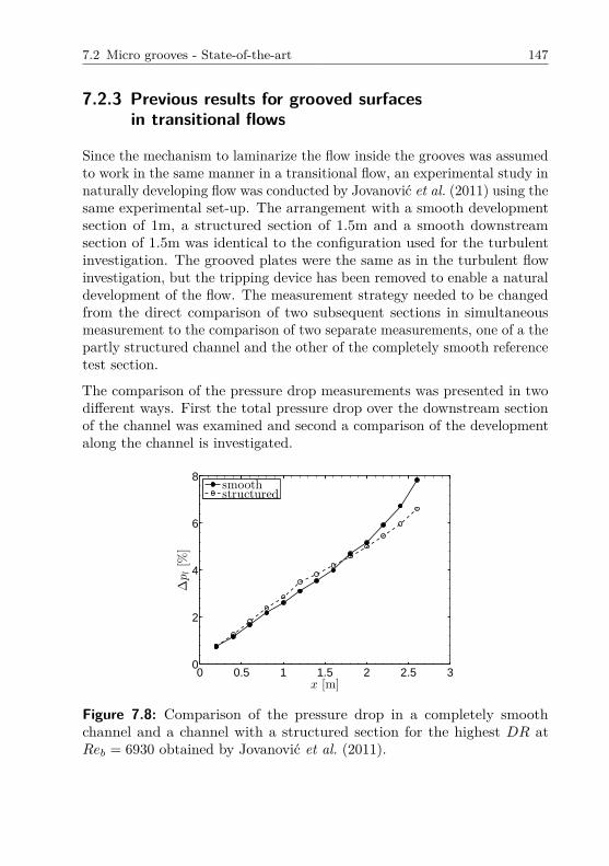
7.2 Micro grooves - State-of-the-art 147
7.2.3 Previous results for grooved surfacesin transitional flows
Since the mechanism to laminarize the flow inside the grooves was assumedto work in the same manner in a transitional flow, an experimental study innaturally developing flow was conducted by Jovanovic et al. (2011) using thesame experimental set-up. The arrangement with a smooth developmentsection of 1m, a structured section of 1.5m and a smooth downstreamsection of 1.5m was identical to the configuration used for the turbulentinvestigation. The grooved plates were the same as in the turbulent flowinvestigation, but the tripping device has been removed to enable a naturaldevelopment of the flow. The measurement strategy needed to be changedfrom the direct comparison of two subsequent sections in simultaneousmeasurement to the comparison of two separate measurements, one of a thepartly structured channel and the other of the completely smooth referencetest section.
The comparison of the pressure drop measurements was presented in twodifferent ways. First the total pressure drop over the downstream sectionof the channel was examined and second a comparison of the developmentalong the channel is investigated.
0 0.5 1 1.5 2 2.5 30
2
4
6
8
x [m]
∆pl[%
]
smoothstructured
Figure 7.8: Comparison of the pressure drop in a completely smoothchannel and a channel with a structured section for the highest 𝐷𝑅 at𝑅𝑒𝑏 = 6930 obtained by Jovanovic et al. (2011).

148 7 Micro grooves
Figure 7.8 (adopted from Jovanovic et al. (2011)) shows the pressure dropalong the channel for a smooth and a partly structured surface conditionat 𝑅𝑒𝑏 = 6930. Note that the length of the development section plus thedistance to the first pressure tap, in sum 0.7m, is not included in the data.Thus data presentation starts directly on the structured plate. The pressuredrop on the grooved surface is slightly larger than on the structured platefor 𝑥 < 1.5m. While the pressure follows a laminar development almost tothe end of the channel downstream the grooved surface, it increases in thedownstream section of the completely smooth channel. The plot depicts thesituation for the highest 𝐷𝑅 found at 𝑅𝑒𝑏 = 6930. For a narrow range of𝑅𝑒𝑏 a delay of the transition is obtained. For smaller and larger Reynoldsnumbers the grooves have no influence on the flow, which is in agreementto the findings in turbulent flow.
As a result, the partly structured channel exhibits a smaller pressure loss,but drag reduction is not found, where the grooves are located. In contrast,the skin friction is little higher on the structured section. Jovanovic et al.(2011) explain the increase of pressure drop in the structured part of thetest section as the interaction of the microgroove structures with near-walldisturbances. This would lead to a stabilizing effect and prevent the growthof disturbances in the near wall region. Therefore the flow would developlaminar over the downstream smooth section.
Furthermore, Jovanovic et al. (2011) presented a comparison of the turbu-lence level close to the channel outlet. Separate plots for the grooved andthe smooth surface were shown, each for increasing and decreasing flowrate. A significant hysteresis effect between the increasing and decreasingcase is observed for both surface conditions. It is concluded that for theverification of a transition delay the shift of the transition to higher 𝑅𝑒needs to be achieved for identical inlet conditions with increasing flow rate(Jovanovic et al., 2011).
To allow a direct comparison of the data for increasing flow rate, the presentauthor has adopted the data of both surface conditions from Jovanovic et al.(2011), which is shown in Figure 7.9. The laminar-turbulent transition isclearly visible in each curve. The position of maximum turbulence intensityis nearly equal for both surface conditions. Only for low Reynolds numbersthe results differ slightly. The turbulence intensity grows continuously forthe smooth surface condition, whereas it rather stagnates before risingabruptly at 𝑅𝑒𝑏 = 6000 for the grooved surface condition. In the fullyturbulent regime, the curves almost coincide. Comparing these two curves

7.3 Experimental investigation of micro grooves 149
0 5000 10000 15000 200000
2
4
6
8
10
Reb
Tu[%
]
smooth increasing flow rategrooved increasing flow rate
Figure 7.9: Comparison of the turbulnce level for increasing flow rate for acomplete smooth channel and a channel with a structured section (adoptedfrom Jovanovic et al. (2011)).
in the fully turbulent part, Jovanovic et al. (2011) illustrate a shift of thestate of fully developed turbulent flow to higher 𝑅𝑒 in the grooved channel.This interpretation of the data is not shared by the author as a significantshift is not visible in Figure 7.9. For 𝑅𝑒𝑏 > 9000 the observed turbulencelevel is the same for both surface conditions.
7.3 Experimental investigation of micro grooves
The literature data indicated the effective groove width in turbulent flowat very small scaling of 𝑎+ = 0.8 with corresponding Reynolds numberbeing close to a still transitional regime (cf. (Frohnapfel et al., 2007a)).Thus the goal is to produce slightly smaller structures to guarantee a fullyturbulent flow conducting the experiments at higher 𝑅𝑒. Identical grooveshave shown to be effective in transitional and turbulent flow for significantlydifferent 𝑅𝑒𝑏, resulting in a different scaling in wall units. Therefore a smalldifference in the groove size is assumed not to change the effectiveness.
The rectangular grooves are shown to reduce skin friction drag inFrohnapfel (2006), although the geometry exhibits two friction gener-

150 7 Micro grooves
ating hot-spots at the edges. Further improvement of the effectivenesswas intended by a smaller angle of the groove flank with using V-shapedgeometry.
7.3.1 Fabrication of the groove structures
The fabrication of the grooves turned out to be quite difficult. The chal-lenging task was to produce the geometry on such a large surface areawithin the specified accuracy. Most micro-machining applications and inconsequence the machine tools are also of small size. Precise manufacturingis usually limited to few centimeters with an enormous time effort. Forexample, micro-milling produced very good results, but to structure a plateof 1500mmx300mm would have taken two months.
s=300µma=100µmh=
95µ
m82µ
m
298µm150µm
Figure 7.10: Dimensions of rectangular and V-shaped grooves.
To resolve these issues, the structures have been successfully manufacturedby broaching aluminum plates. The fabrication has been conducted at theInstitute PTW at TU Darmstadt. It has been possible to produce threesegments of 500mm length. A conventional milling machine was equippedwith a custom built broaching tool, which allowed to simultaneously broach18 parallel grooves. The best results were obtained for plates of high-strength aluminum. The surface needed to be machined two times toachieve the required depth of the grooves with a high-quality surface finishinside the grooves. Two different grooves types were realized: a triangularand a square groove shape. After the broaching process significant burrs

7.4 Measurements in turbulent flow 151
occurred along the upper edges of the grooves for the rectangular geometry.These plates were sanded until the burrs had been removed without adetectable removal on the smooth surface between the grooves. The finalgeometry of both groove geometries is shown in 7.10. In both cases thegeometry is very precise. The deviation of the groove depth and spacinghave been checked with a microscope to have a tolerance of only ±2𝜇m.The sidewalls of the rectangular grooves are nearly normal to the horizontalbottom surface (89.6∘).
7.3.2 Measurement strategy
For the transitional as well as for the turbulent study measurements in thechannel with a partly structured surface were compared to the correspondingcomplete smooth reference data, which are shown in Chapter 5. In bothmeasurement campaigns the humidity has not been taken into account.Therefore measurement accuracy is decreased in comparison to the ribletstudy. A measurement accuracy of changes in 𝜏𝑤/𝜏𝑤,0 of 2% for 𝑅𝑒𝑏 < 4000increasing to slightly less than 1% at 𝑅𝑒𝑏 ≥ 8000 is possible. Consideringthe expected large amount of 𝐷𝑅 = 10 − 20% on the structured surface,this is still appropriate.
7.4 Measurements in turbulent flow
For the measurements in turbulent flow the surfaces structured with rect-angular grooves were installed in the downstream part of the channel toguarantee a fully turbulent flow at preferably low 𝑅𝑒. The 13% trippinghas been used.
Figure 7.11 compares the pressure drop of the reference measurementwith smooth surface to the results obtained with a grooved section in thedownstream part of the channel. In total the plots consists of 450 datapoints. Although it is not visible in this presentation due to the very goodmatching, the filled symbols at higher 𝑅𝑒𝑏 are not single measurements, butwere repeated between four to six times. The entire 𝑅𝑒 range was checkedin very smalls steps of the flow rate, but since no difference was obtained,measurements were concentrated more in promising low 𝑅𝑒 range.

152 7 Micro grooves
987654323
x
Figure 7.11: Comparison of the pressure loss in a complete smooth channeland a channel with a structured section in dependence of 𝑅𝑒𝑏.
From the evolution of the pressure drop results the range of laminar (𝑅𝑒𝑏 <2500), transitional and turbulent flow (𝑅𝑒 > 4000) can be differentiated.For the laminar as well as for the turbulent regime the data show the sameresult for both surface conditions. Only in the highly transitional state,for 2600 < 𝑅𝑒𝑏 < 3000 a small differences between smooth and structuredsurface can be conjectured.
For the transitional regime it was mentioned in Chapter 5.3, that theenvironmental noise had an influence on the pressure loss (up to 3%).Therefore, the measurements in the transitional region were completelyrepeated under absolute quiet conditions for the grooved as well as for thereference surface. The test section has been reassembled changing betweenthe two surface conditions. Figure 7.12 focuses on the measurements in thetransitional region. The data show the 𝑐𝑓 -value instead of the pressure lossto exclude slight deviation between different measurements originating fromthe changes in the air properties. The high reproducibility confirms theestimated measurement uncertainties of approximately 2% at low 𝑅𝑒 andis in the range of 1% for 𝑅𝑒𝑏=3500. In the transitional regime a naturally
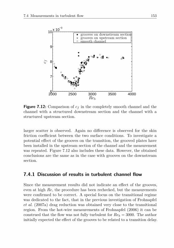
7.4 Measurements in turbulent flow 153
2000 2500 3000 3500 40006
7
8
9
10x 10
−3
Reb
cf
grooves on downstream sectiongrooves on upstream sectionsmooth channel
Figure 7.12: Comparison of 𝑐𝑓 in the completely smooth channel and thechannel with a structured downstream section and the channel with astructured upstream section.
larger scatter is observed. Again no difference is observed for the skinfriction coefficient between the two surface conditions. To investigate apotential effect of the grooves on the transition, the grooved plates havebeen installed in the upstream section of the channel and the measurementwas repeated. Figure 7.12 also includes these data. However, the obtainedconclusions are the same as in the case with grooves on the downstreamsection.
7.4.1 Discussion of results in turbulent channel flow
Since the measurement results did not indicate an effect of the grooves,even at high 𝑅𝑒, the procedure has been rechecked, but the measurementswere confirmed to be correct. A special focus on the transitional regimewas dedicated to the fact, that in the previous investigation of Frohnapfelet al. (2007a) drag reduction was obtained very close to the transitionalregion. From the hot-wire measurements of Frohnapfel (2006) it can beconstrued that the flow was not fully turbulent for 𝑅𝑒𝑏 = 3000. The authorinitially expected the effect of the grooves to be related to a transition delay.

154 7 Micro grooves
Although a delay of transition could not be observed, the explanation forthe 𝐷𝑅 in the former turbulent investigations may be related to a not fullyturbulent flow.
A consideration of the flow development highlights a possible explanationfor the discrepancy between the similar investigations in different testfacilities: Even if 𝑅𝑒𝑏 is slightly above the fully turbulent limit at thechannel outlet, a considerable length of laminar to transitional flow inthe tunnel entrance region can be conjectured. In the present facility thiswas demonstrated in the reference measurement in Chapter 5 and it isshown explicitly in Figure 5.9(b), where most of the channel length showsa laminar flow development. The observation remained similar also for the16% tripping, where the flow at the outlet was already fully turbulent atthe smallest considered 𝑅𝑒 (compare Fig. 5.10).
In Figure 7.13 the original data from Frohnapfel et al. (2007a) are plottedon the left hand side and the data from the smooth reference of the presentstudy on the right hand side. Since the development length of 700mm fromthe channel entrance was not studied in the Frohnapfel’s investigation andthe present channel is 0.5m longer, these additionally investigated sectionsin the present investigation are shaded in grey. The lines indicate the meanpressure gradient on the smooth and the structured segments. The slightlydeviating tripping device and the differing channel height (35mm and25mm) lead to differences in the flow development at the same 𝑅𝑒𝑏 betweenthe two experimental set-ups. Additionally, the crucial differences in thedetermination of 𝑅𝑒𝑏 induce considerable uncertainty to the comparabilityof the Reynolds number (cf. Appendix A.1). While even at very low flowrates the present instrumentation has a measurement accuracy better than±1.5% for 𝑅𝑒𝑏, the uncertainty of 𝑅𝑒𝑏 is specified with ±10% in Frohnapfel(2006) for very low 𝑅𝑒. Thus corresponding states of flow development arecompared. Note that the diagrams on the left-hand side do not depict thephysical pressure loss but the voltage output of the pressure transducerat varying measurement ranges of the sensor as given by Frohnapfel et al.(2007a).
The comparison of the larger Reynolds numbers (𝑅𝑒𝑏 = 3620 and 3940,respectively) shows a more or less constant pressure drop in the consideredpart of the test section. The diagram (f) for 𝑅𝑒𝑏 = 3940 indicates a laminarregion at the beginning of the channel (within the shaded section). For𝑅𝑒𝑏 = 3300 (d) the laminar region propagates far into the channel resultingin a smaller gradient in the downstream section than in the upstream

7.4 Measurements in turbulent flow 155
0 0.5 1 1.5 2 2.5 30
0.01
0.02
0.03
0.04
0.05
0.06
0.07
0.08
x [m]
∆E
[V]
groovedsmooth
(a) 𝑅𝑒𝑏 = 2450 (b) 𝑅𝑒𝑏 = 2640
0 0.5 1 1.5 2 2.5 30
0.02
0.04
0.06
0.08
0.1
0.12
x [m]
∆E
[V]
groovedsmooth
(c) 𝑅𝑒𝑏 = 2870 (d) 𝑅𝑒𝑏 = 3300
0 0.5 1 1.5 2 2.5 30
0.02
0.04
0.06
0.08
0.1
0.12
0.14
0.16
x [m]
∆E
[V]
groovedsmooth
(e) 𝑅𝑒𝑏 = 3620 (f) 𝑅𝑒𝑏 = 3940
Figure 7.13: Comparison of the pressure drop for the complete test sections.Data with the upstream section equipped with grooves are replotted fromFrohnapfel et al. (2007a) in the left column. The smooth reference ofthe present measurement are shown in the right column for different 𝑅𝑒𝑏.Dashed lines depict the mean pressure gradient on upstream and continuouslines on the downstream section.

156 7 Micro grooves
section. This finding is very similar to 𝑅𝑒𝑏 = 2870 (c), which depicts thedata for the highest 𝐷𝑅 from Frohnapfel et al. (2007a). For even lower𝑅𝑒𝑏, Figures 7.13 (b) depicts the flow development for a Reynolds number,where the hot-wire measurement at the channel outlet still indicated a highturbulence level. Although the flow is transitional for most of the channellength, the pressure gradient along the channel is approximately constant,if the sections shaded in grey are not taken into account. Figures 7.13 (a)shows the corresponding data from Frohnapfel et al. (2007a).
Determining the drag reduction by an evalution of the ratio of the meanpressure gradient along the upstream and downstream plate as done byFrohnapfel et al. (2007a), a significant drag reduction would be construedfor both situation in Figures 7.13 (c) and (d). However, it can be clearlyseen from the present data that the different gradients are exclusivelya result of the flow development in the channel. This also can explainwhy Frohnapfel only obtained drag reduction in the case of grooves in theupstream section. The observation of a smaller gradient in the downstreampart is also observed for a completely smooth channel by Frohnapfel et al.(2007a) at 𝑅𝑒𝑏 = 2850, which is very close to 𝑅𝑒𝑏 = 2870 of maximum 𝐷𝑅with the structured surfaces (compare Fig. 7.13 (c)).
The increase of the drag reduction for different channel heights can beinterpreted as follows. Note that at the same flow rate channels of arbitraryheight exhibit the same Reynolds number (for a constant channel width 𝑊 ),thus 𝑅𝑒𝑏 = 𝑓(𝐻). Yet, the flow development is a function of the channelheight, meaning that with increasing channel height, the required physicaldevelopment length is longer for a given 𝑅𝑒𝑏. Hence, the transitional length,which is found at the channel entrance for low 𝑅𝑒 even with the trippedflow, can probably extend further into the channel for larger 𝐻 and thus theapparent 𝐷𝑅 is increased. These considerations can explain the increased𝐷𝑅 from a 𝐻 = 25mm to 𝐻 = 35mm in Frohnapfel (2006) (compare Fig.7.6). The same tendency can be construed from the significantly larger 𝐷𝑅reported by Jovanovic et al. (2010a) with a channel configuration using𝐻 = 41mm. As soon as the Reynolds number is large enough to enablean abrupt turn to a turbulent state, a running length of 700mm will besufficient to obtain a fully turbulent flow. Due to the required developmentlength, which was found to be in range of 𝐻 = 70 − 80 a comparison ofthe pressure gradient on the downstream and upstream section will showonly slightly smaller values for the downstream section. This is indicatedin a comparison of pressure drop on the two section of a complete smoothchannel shown by Frohnapfel et al. (2007a) for higher Reynolds numbers.

7.5 Measurements in transitional flow 157
In summary, the drag reduction due to micro grooves, as reported by ofFrohnapfel et al. (2007a) could not be confirmed by the numerous moresophisticated and more accurate measurements. A significant effect of thegroove structures on turbulent channel flow could not be verified.
7.5 Measurements in transitional flow
0 2000 4000 6000 8000 10000 120003
4
5
6
7
8x 10
−3
Reb
cf
complete smoothwith grooved section
Figure 7.14: 𝑐𝑓 over 𝑅𝑒𝑏 for complete smooth and partly grooved surfacefor naturally developing flow.
In the previous measurements the rectangular grooves were shown to bepractically effectless in turbulent flow. In general, the V-shaped grooveswere supposed to be more effective, since the friction generating upperedges at the groove flanks are reduced in angle. To maximize any possibledrag reduction effect in transitional flow, the V-shaped geometry is used forthis more difficult investigation in which the flow is developing completelynaturally, i.e. no tripping is used. The channel configuration is similar tothe one presented by Jovanovic et al. (2010a): A smooth entrance section of950mm length is followed by a 1500mm segment with the structured surfaceand the downstream section of 1500mm is again smooth. The difference tothe measurement by (Jovanovic et al., 2010a) is the length of the smooth

158 7 Micro grooves
0 1 2 3 40
1
2
3
4
5
6
x [m]
∆pl[Pa]
smoothgrooved
(a) 𝑅𝑒𝑏 = 4250
0 1 2 3 40
2
4
6
8
10
x [m]
∆pl[Pa]
smoothgrooved
(b) 𝑅𝑒𝑏 = 5820
0 1 2 3 40
2
4
6
8
10
x [m]
∆pl[Pa]
smoothgrooved
(c) 𝑅𝑒𝑏 = 6200
0 1 2 3 40
10
20
30
40
x [m]
∆pl[Pa]
smoothgrooved
(d) 𝑅𝑒𝑏 = 10000
Figure 7.15: Comparison of the pressure drop for the completely smoothtest section and the one with a grooved section for different 𝑅𝑒𝑏.

7.5 Measurements in transitional flow 159
0 1 2 3 40
2
4
6
8
10
12
14
x [m]
∆pl[P
a]
smoothsmoothgroovedgrooved
Figure 7.16: Pressure drop for the transitional regime at 𝑅𝑒𝑏 = 6320 fordifferent measurements.
0 5000 10000 150000
2
4
6
8
10
12
Reb
Tu[%
]
smooth increasing V
grooved increasing V
Figure 7.17: Turbulence level for increasing and decreasing 𝑅𝑒𝑏.

160 7 Micro grooves
section at the channel entrance, which is 450mm longer than the 500msection used by Jovanovic et al. (2010a).
Figure 7.14 shows the skin friction coefficient over 𝑅𝑒𝑏 for the completelysmooth channel and the channel configuration with a structured section.Strikingly, very similar results are obtained for both surface conditions forall Reynolds numbers. In the range of 5000 < 𝑅𝑒𝑏 < 6000 few scatteringdata points indicate how slight environmental noise can trigger prematuretransition, leading to an increase of the skin friction. Generally, scatterin the data is larger in transitional range. It decreases significantly for𝑅𝑒𝑏 > 9000, the Reynolds number range where the flow directly developsturbulent.
To identify possible differences in the streamwise flow development, Figure7.15 presents the pressure drop along the channel with a grooved section incomparison to the data of the smooth reference channel presented in Chapter5.1 for different 𝑅𝑒. In all cases a nearly perfect agreement of data of thestructured and smooth plates is observed. In the transitional region morescatter of the data was found, since very small differences in the 𝑅𝑒 causelarge differences in the pressure drop. Even the temporal evolution plays arole. For a narrow Reynolds number range (6100 < 𝑅𝑒𝑏 < 6700), it wasfound that the transition can vary slightly towards the turbulent or towardsthe laminar flow state during long-time measurements. However, this effectcould only be observed in a narrow range of 𝑅𝑒. Figure 7.16 examplarilyshows four measurements for the 𝑅𝑒 at which very high turbulence levelat the channel outlet was obtained. Two measurements with completelysmooth surfaces and two measurements with partly structured channelwalls are compared for the same Reynolds number (𝑅𝑒𝑏 = 6320). At thechannel entrance the development of all four measurements is very similar.At the half length of the channel there are small deviations, although thetotal pressure loss is almost the same in all cases. Even for this highlytransitional state, significant differences in the flow development dependingon the surface conditions are not observed.
To exclude an influence of an improper adjustment of the test plates duringthe assembly, the channel configuration has continuously been changedbetween the smooth and structured surface. The presented measurementsare part of the data gathered over a period of four months. Note that thereis no indication of an influence of the test plate intersections in any of thedata sets. As mentioned in Chapter 5.1, the pressure tab at 2m did notwork properly, but is shown since the deviation is small and reproducible.

7.5 Measurements in transitional flow 161
The measurement of the turbulence level showed the same result for bothsurface conditions for increasing flow rate (see Fig. 7.17). For decreasingflow rate the result differs significantly between the measurements. Itseems that even for very calm conditions the turbulence level can decreaserapidly with only little difference to the increasing flow rate. In othermeasurements the flow remained turbulent to much smaller 𝑅𝑒𝑏 similarto the result shown by (Jovanovic et al., 2011). The process in decreasingflow rate seems to be stochastic to some degree and it is very difficult toobtain a single representative curve. Such measurement for decreasing flowrate has been repeated several times, but a precisely reproducible curvewas not found.
7.5.1 Discussion of transitional resultsin transitional channel flow
The present results clearly show an identical behavior of the smooth refer-ence and the channel equipped with grooved plates. The structured platesbehave like hydraulically smooth surfaces for the investigated Reynoldsnumber range. Therefore, this result does not confirm previous findingsconcerning the drag reduction.
In the following differences in the experimental set-ups are pointed out andpossible reasons for the differing results are concluded.
The geometry of the structures is differing between both studies. Thegrooves in the present study are slightly smaller and the curvature is V-shaped instead of rectangular. With these changes it was intended toincrease the effectiveness of the structures. Despite these differences, it isremarkable, that there was no indication of a smallest difference in thewall shear stress between the reference and grooved surface in the presentinvestigation.
The turbulence level for increasing flow rate showed no significant differencesbetween the differing surface condition in the study by Jovanovic et al.(2011) as well as in the present one. But the maximum peak of theturbulence level of naturally developing flow seems to occur at different𝑅𝑒𝑏 in the two studies. In this particular case the difference is a result ofthe different calculation of the flow rate. In the measurements obtainedin Erlangen the flow rate was calculated using the Bernoulli equation (cf.Spiegel (2013), Frohnapfel (2006)). This computation overestimates the
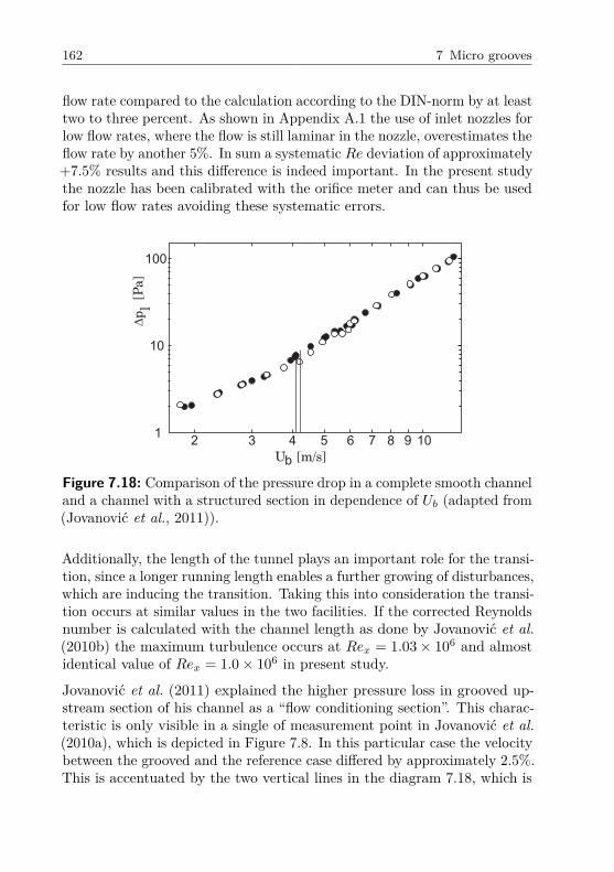
162 7 Micro grooves
100
10
12 3 4 5 1096 7 8
U [m/s]b
Dp
[
Pa]
l
Figure 7.18: Comparison of the pressure drop in a complete smooth channeland a channel with a structured section in dependence of 𝑈𝑏 (adapted from(Jovanovic et al., 2011)).
Additionally, the length of the tunnel plays an important role for the transi-tion, since a longer running length enables a further growing of disturbances,which are inducing the transition. Taking this into consideration the transi-tion occurs at similar values in the two facilities. If the corrected Reynoldsnumber is calculated with the channel length as done by Jovanovic et al.(2010b) the maximum turbulence occurs at 𝑅𝑒𝑥 = 1.03 × 10⁶ and almostidentical value of 𝑅𝑒𝑥 = 1.0 × 10⁶ in present study.
Jovanovic et al. (2011) explained the higher pressure loss in grooved up-stream section of his channel as a “flow conditioning section”. This charac-teristic is only visible in a single of measurement point in Jovanovic et al.(2010a), which is depicted in Figure 7.8. In this particular case the velocitybetween the grooved and the reference case differed by approximately 2.5%.This is accentuated by the two vertical lines in the diagram 7.18, which is
flow rate compared to the calculation according to the DIN-norm by at leasttwo to three percent. As shown in Appendix A.1 the use of inlet nozzles forlow flow rates, where the flow is still laminar in the nozzle, overestimates theflow rate by another 5%. In sum a systematic 𝑅𝑒 deviation of approximately+7.5% results and this difference is indeed important. In the present studythe nozzle has been calibrated with the orifice meter and can thus be usedfor low flow rates avoiding these systematic errors.

7.5 Measurements in transitional flow 163
adopted from Jovanovic et al. (2011). If we consider a quadratic relationof the pressure drop on 𝑈𝑏, an 2.5% higher velocity results in an increaseof the pressure drop of 5% (assuming exactly the same air properties).Figure 7.8 compares the pressure drop along the test section for bothcases. As expected for the flow of higher velocity (grooved surface) thepressure drop is larger on the upstream part of the channel, where the flowis laminar in both cases. On the downstream part of the channel the flowin the complete smooth channel develops turbulent at 𝑥 > 1.8𝑚, whilethe flow downstream the grooved surfaces remains laminar. Therefore, themeasurement with higher velocity leads to less total pressure loss. Thisexplanation to the different pressure drop on the upstream section seemsmuch more plausible.
A general question concerning transition investigations in channel flowremains: Is a tunnel with an moderate aspect ration of 12 appropriate forthis kind of testing?
The length of the channel may be large enough, that the transition-triggeringdisturbances are mainly self-generated by the side wall effects (secondaryflow), as it was reported by Dean (1978). At a certain downstream distancethe growing corner vortex structures observed in laminar flow throughducts interact with each other forming new disturbances. The very exactreproducibility of the onset of transition with the present set-up, mayprobably be a result of this. The observations of Arbeiter (2009) supportsuch considerations (compare Chap. 2.2.3).


8 Spanwise oscillating wallsimplemented via dielectricelastomer actuators
This chapter presents the implementation of an active flow control techniquein the present experimental set-up. The chosen technique of spanwise walloscillation is promising in two aspects: a considerably large reduction ofthe mean streamwise skin-friction drag is obtained (Quadrio & Ricco, 2004)and the wall oscillations are a predetermined control strategy, meaningthat the control action is defined a priori and does not depend on the flowstate. Thus, compared to other active approaches, the wall oscillations areof moderate complexity, since neither complex control circuits nor sensorsare required. The challenging task is the energy efficient implementationof large oscillating areas.
Recently, Gouder et al. (2013) presented an experimental study using anovel actuator concept for realization of spanwise wall movement: thedielectric electroactive polymers. The dielectric elastomer actuators exhibitseveral advantages in comparison to conventionally used approaches, wherethe walls are driven electrically or electromagnetically:
∙ They are capable of exerting in-plane, unidirectional oscillations.
∙ The lightweight devices comply with the requirements for flow controlapplications.
∙ The power consumption is low.
Although a preliminar study by Gouder et al. (2013) has shown thatdrag reduction by spanwise wall oscillations with dielectric polymer basedactuators can be achieved, the technology was judged to be unattractivedue to the fragility of the actuators. The lifetime of only a few minutes(Gouder, 2011) limited the possibility to experimentally study the DEA inthe wind tunnel.

166 8 Spanwise oscillating walls implemented via dielectric elastomer actuators
ds
Figure 8.1: Stokes layer generated by cyclic movement of the wall.
The present study evolved from a cooperation with Davide Gatti, whoadvanced a new approach for the implementation of wall oscillations viadielectric electroactive polymers. Details of the material properties and theactuator design can be found in Gatti (2014b). The present wind-tunnelfacility represents the perfect framework for testing these new devices forspanwise wall oscillations. While a detailed comparison of the measurementdata to numerical simulations is presented in Gatti (2014b), the scope ofthe present work is to introduce and verify the experimental procedure.
In the following the concept of spanwise oscillating walls is introduced.Subsequently the working principle of a DEA and its application for theconstruction of a DEA actuator is shown. The challenges of implementingthe DEA actuators in the experimental set-up are discussed. The measure-ment results are presented and the Chapter is completed with a discussionof the results.
8.1 Spanwise oscillating walls
An in-plane, oscillatory motion of the wall corresponds to the impositionof a periodic wall velocity 𝑢𝑤 as follows:
𝑢𝑤(𝑡) = 𝐴𝑚 sin(
2𝜋
𝑇𝑡
)with 𝑇 = 2𝜋
𝜔(8.1)

8.1 Spanwise oscillating walls 167
In equation (8.1) 𝐴𝑚 is the amplitude, 𝑇 the period and 𝜔 the angularfrequency of the oscillation. Consequently to the periodic spanwise wallvelocity due to the no-slip condition, a periodic flow is created above thewall, which is confined to the so-called Stokes layer in a distance 𝛿𝑆 fromthe wall. The velocity profile for different phases of one period of the wallmovement is sketched in Figure 8.1. The flow within the Stokes layer canbe described by an analytic solution for the laminar case (Schlichting &Gersten, 2000):
𝑢𝑤(𝑥2, 𝑡) = 𝐴𝑚 exp(
−𝑥2
√𝜋
𝑇𝜈
)sin
(2𝜋
𝑇𝑡 − 𝑥2
√𝜋
𝑇𝜈
)(8.2)
Drag reduction can be achieved, if spanwise wall oscillations are superposedto a turbulent wall-bounded flow. Vittori & Verzicco (1998) found thatthe main flow and the cross flow effectively interact only if the Reynoldsnumber 𝑅𝑒𝛿, based on the thickness of the Stokes layer 𝛿𝑆 and the oscillationamplitude 𝐴𝑚, 𝑅𝑒𝛿 = 𝐴𝑚𝛿𝑆
𝜈 is smaller than 120. For this Reynolds numberthe cross flow in calm air would be laminar.
Since the seminal work of Jung et al. (1992), in which wall oscillationshave been numerically proved to lead to turbulent drag reduction, a largenumber of numerical studies followed (Baron & Quadrio, 1996; Choi et al.,2002; Duque-Daza et al., 2012; Gatti & Quadrio, 2013; Quadrio & Ricco,2003, 2004; Quadrio & Sibilla, 2000; Ricco & Quadrio, 2008; Touber &Leschziner, 2012; Yakeno et al., 2014). Probably, the most comprehen-sive numerical study on the effect of oscillating walls was presented byQuadrio & Ricco (2004). DNS of turbulent channel flow at low 𝑅𝑒 havebeen exploited to investigate the optimal oscillations parameters and theimportant role of the oscillation period 𝑇 was found. A optimal periodin a range of 𝑇 +=100 to 120 was found, where 𝑇 + is calculated with thefriction velocity 𝑢𝜏,0 of the reference flow and the kinematic viscosity 𝜈.A small number of experimental laboratory investigation confirmed thedrag-reducing capabilities of wall oscillaitons (Choi & Clayton, 2001; Choiet al., 1998; Di Cicca et al., 2002; Gouder et al., 2013; Ricco & Wu, 2004;Trujillo et al., 1997).
Despite the large number of investigations the drag reduction mechanismis yet not understood. The different approaches to explain the mechanismare discussed by Gatti (2014b).

168 8 Spanwise oscillating walls implemented via dielectric elastomer actuators
8.1.1 Dielectric electroactive polymers
Figure 8.2 illustrates the basic principle of a DEA. An isolating material,the dielectric, is sandwiched between two conductive compliant electrodes.This ensemble can be interpreted as a parallel plate capacitor. If an electricfield is applied across the dielectric, the electrodes attract each other.The resulting forces exert a pressure on the dielectric, called the Maxwellpressure 𝑝𝑒:
𝑝𝑒 = 𝜖0𝜖𝑟𝐸2
ℎ2 . (8.3)
The Maxwell pressure (Eq. (8.3)) depends on the the vacuum permittivity𝜖0=8.85x10⁻¹²F/m, the relative permittivity of the dielectric 𝜖𝑟, the dis-tance between the electrodes ℎ and the potential difference between theelectrodes 𝐸. In a standard plate capacitor, the stiff electrodes are fixedin a certain position and the deformation due to the Maxwell pressure isnegligibly small. In a DEA the electrodes are of compliant material andapplied on the elastic dielectric medium. In this context compliant meansthat the electrodes can significantly deform while remaining conductive.For the dielectric, a soft elastomeric material is usually used, which ishighly deformable and can be regarded as incompressible. The Maxwellpressure deforms the isolating material. The elastomer is thinned and itssurface area is expanded (Fig. 8.2).
elastomer
compliantelectrodes
pe
l
l + lD
Figure 8.2: Deformation of a DEA material.

8.1 Spanwise oscillating walls 169
8.1.2 Working principle of dielectric elastomer actuators
To exploit the DEA for fluid mechanic applications, an in-plane oscillatorymovement is required. In Figure 8.3 the main actuator arrangement isshown. A pre-stretched elastomeric membrane is clamped between twosupporting frames. On opposite sides two pairs of compliant electrodes areapplied onto the membrane. If the capacitor on the left side is electricallycharged as shown in the upper illustration of Figure 8.3, the Maxwellpressure leads to an elongation of the underlying membrane and a movementtowards the right side is generated. If this capacitor is discharged, whilethe one on the right side is loaded, a movement in the opposite direction isachieved. The pre-stretch of the elastomer is important to avoid an out ofplane movement due to loss of tension of the membrane.
pe
pre-stretchedmembrane
base plate supporting frame
pe
compliantelectrodes
Figure 8.3: Working principle of a DEA.
The basic layout of the actuator for the wind tunnel testing is inspiredby (Gouder et al., 2013). The active membrane is not directly used tomanipulate the flow. It is coupled with a second passive membrane whichconstitutes the surface wetted by the flow. A transfer element, whichis glued on the membranes as depicted in Figure 8.4, directly couplesthe movement of the active and passive membrane. For a lightweightconstruction the transfer elements are made of balsa wood. The movementof the output shaft is illustrated in Figure 8.5. The passive surface isstiffened by a thin plastic plate to ensure a homogenous displacement of a

170 8 Spanwise oscillating walls implemented via dielectric elastomer actuators
Supporting frames
DEAP membrane
Output shaft
Electrode set 1
Electrode
set 2
Interconnection
200
25
30
170
Figure 8.4: Active membrane of the DEA.
Figure 8.5: Illustration of the movement of the output shaft on the activesurface of a DEA.
A large spanwise displacement is only achieved, when the actuator isoperated at its in-plane mechanical resonance frequency. As a consequence,a given actuator design has a fixed working frequency, which depends onthe stiffness of the membrane, the area of the membrane and the pre-stretch. The resonance frequency of actuators for the wind tunnel testingis additionally modified by the weight of the transfer elements and thestiffness of the surface membrane.
In the measurements two types of actuators were used. In Figure 8.6 theactuator type WT1 is shown, which has been developed by Gatti (2014b).It has an actuated length of 230mm in streamwise and spanwise direction.
large part of the actuated surface. An exploded view of the construction isdepicted in Figure 8.6.
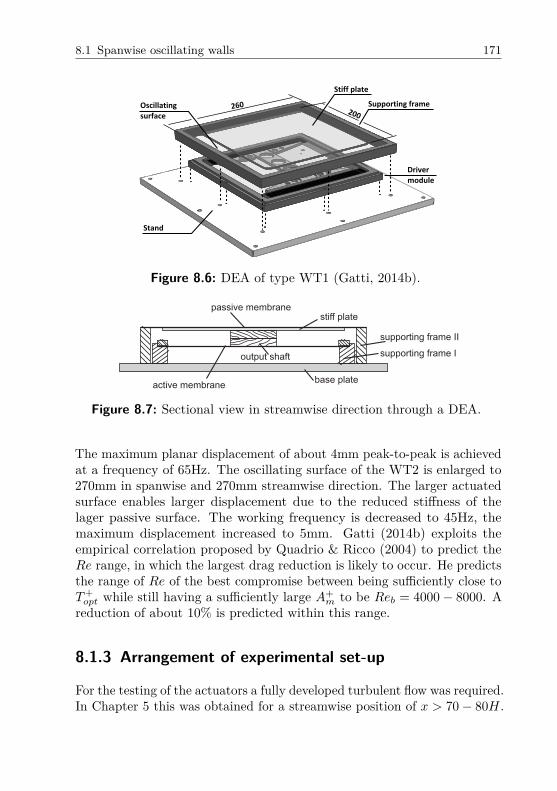
8.1 Spanwise oscillating walls 171
Supporting frameOscillating
surface
Stiff plate
Driver
module
Stand
260200
Figure 8.6: DEA of type WT1 (Gatti, 2014b).
passive membrane
active membranebase plate
stiff plate
supporting frame I
supporting frame II
output shaft
Figure 8.7: Sectional view in streamwise direction through a DEA.
The maximum planar displacement of about 4mm peak-to-peak is achievedat a frequency of 65Hz. The oscillating surface of the WT2 is enlarged to270mm in spanwise and 270mm streamwise direction. The larger actuatedsurface enables larger displacement due to the reduced stiffness of thelager passive surface. The working frequency is decreased to 45Hz, themaximum displacement increased to 5mm. Gatti (2014b) exploits theempirical correlation proposed by Quadrio & Ricco (2004) to predict the𝑅𝑒 range, in which the largest drag reduction is likely to occur. He predictsthe range of 𝑅𝑒 of the best compromise between being sufficiently close to𝑇 +
𝑜𝑝𝑡 while still having a sufficiently large 𝐴+𝑚 to be 𝑅𝑒𝑏 = 4000 − 8000. A
reduction of about 10% is predicted within this range.
8.1.3 Arrangement of experimental set-up
For the testing of the actuators a fully developed turbulent flow was required.In Chapter 5 this was obtained for a streamwise position of 𝑥 > 70 − 80𝐻.
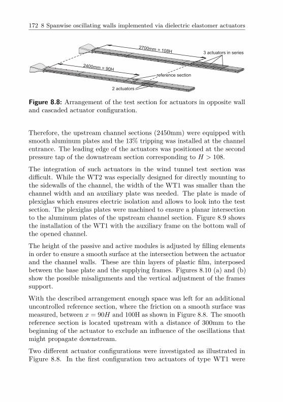
172 8 Spanwise oscillating walls implemented via dielectric elastomer actuators
2700mm = 108H 3 actuators in series
2400mm = 90H
2 actuators
reference section
Figure 8.8: Arrangement of the test section for actuators in opposite walland cascaded actuator configuration.
Therefore, the upstream channel sections (2450mm) were equipped withsmooth aluminum plates and the 13% tripping was installed at the channelentrance. The leading edge of the actuators was positioned at the secondpressure tap of the downstream section corresponding to 𝐻 > 108.
The integration of such actuators in the wind tunnel test section wasdifficult. While the WT2 was especially designed for directly mounting tothe sidewalls of the channel, the width of the WT1 was smaller than thechannel width and an auxiliary plate was needed. The plate is made ofplexiglas which ensures electric isolation and allows to look into the testsection. The plexiglas plates were machined to ensure a planar intersectionto the aluminum plates of the upstream channel section. Figure 8.9 showsthe installation of the WT1 with the auxiliary frame on the bottom wall ofthe opened channel.
The height of the passive and active modules is adjusted by filling elementsin order to ensure a smooth surface at the intersection between the actuatorand the channel walls. These are thin layers of plastic film, interposedbetween the base plate and the supplying frames. Figures 8.10 (a) and (b)show the possible misalignments and the vertical adjustment of the framessupport.
With the described arrangement enough space was left for an additionaluncontrolled reference section, where the friction on a smooth surface wasmeasured, between 𝑥 = 90𝐻 and 100H as shown in Figure 8.8. The smoothreference section is located upstream with a distance of 300mm to thebeginning of the actuator to exclude an influence of the oscillations thatmight propagate downstream.
Two different actuator configurations were investigated as illustrated inFigure 8.8. In the first configuration two actuators of type WT1 were

8.1 Spanwise oscillating walls 173
Figure 8.9: Integration of a WT1 on the bottom wall of the test section.
displacement at the intersection
(a)
filler elements
displacement of active surface
(b)
Figure 8.10: Vertical misalignment of the support frame of the passivemembrane (a) and of the stiffening plate (b).

174 8 Spanwise oscillating walls implemented via dielectric elastomer actuators
located on opposite walls. In the second configuration three actuators werecascaded only on the upper wall. A total streamwise actuator length of900mm is generated. The actuated length was slightly smaller with 840mm,since the actuation is interrupted at the intersection between the devices.
8.1.4 Measurement strategy
The challenging aspect in testing the dielectric elastomer actuators wasthe short streamwise length of 230mm to 270mm of the actuated surface.Since the most effective operation of the actuators is predicted for 4000 <𝑅𝑒𝑏 < 8000, the pressure drop along such a small streamwise distance(200mm) is between 0.6Pa and 2Pa. To detect changes in the skin-frictionwith an accuracy better 1%, pressure changes of smaller 0.01Pa need to bemeasured.
From the reference measurement in turbulent flow of the riblet campaign,it can be concluded that d𝑝/d𝑥 is almost independent of the regardedchannel length (compare Fig. 6.9). The deviation of the single data pointsalong the channel length from a constant slope is extremely small, sincethe variation of the flow rate in time is very small for 𝑅𝑒𝑏 > 5000. It canbe assumed that the measurement accuracy will be not be affected by thesmall regarded streamwise length, which is proofed by the measurementdata shown at the end of this Chapter.
The pressure drop across both the actuator and the reference section havebeen measured repeatedly in six sessions of three minutes averaging timeeach, alternating actuator activation and deactivation. The change in𝜏𝑤 is detected on the smooth and the oscillating surface. The smoothreference surface is needed to verify that the actuation does not influencethe upstream flow. To allow a simultaneous measurement one Baratronsensor has been used for the reference section and the other one for thesegment with the actuators.
In spite of the challenges of measuring small pressure drops across a smallsection, the testing of the active devices offers particular advantages thatimprove the measurement accuracy of 𝜏𝑤/𝜏𝑤,0. Firstly, to investigatethe effect of the wall oscillations, only the actuator needs to be switchedon and off. A reassembly of the test section for the reference case isnot required. The switch between actuator on and off leads to almostthe same favorable situation for the measurement accuracy as the direct

8.2 Measurement results 175
comparison in Chapter 6. The measurement can be conducted within shorttime and thereby deviations of the ambient quantities are negligibly small.Also time dependent deviations of the pressure sensors, both for flow ratemeasurement and pressure drop measurement become very small, since awhole test series can be conducted within one day. Additionally, at thistime the wind tunnel instrumentation was improved to the the final stepof development with a more precise determination of calculation of the airdensity and viscosity.
The calculation of the measurement uncertainty has been adapted for thementioned boundary conditions and the uncertainty intervals shown in thefollowing section represent this result.
8.2 Measurement results
8.2.1 Measurement of reference case
4000 6000 8000 10000 12000 14000 160006
7
8
9
10x 10
−3
ReB [−]
Cf [
−]
Figure 8.11: Determination of 𝑐𝑓 on the smooth reference section (filledsymbols) and the section with the deactivated actuator (open symbols) fromsimultaneous measurement. Circles depict results of the fist measurementseries. Diamonds depict results of the second measurement series.
The data in Figure 8.11 show a comparison of the skin-friction coefficientover the smooth reference surface to the Dean’s law, which was found todescribe very accurately the relation among 𝑐𝑓 and 𝑅𝑒 for the present

176 8 Spanwise oscillating walls implemented via dielectric elastomer actuators
channel in Chapter 5.2. Additionally, the diagram includes data for theactuator section without oscillation with two WT1 actuators in oppositewall configuration. Two different measurement series are included in theplot. For the smooth channel section the skin friction coefficient agreesvery well with both Dean’s law and with the measurements presented inChapter 5.2. The membrane surfaces show good agreement for small 𝑅𝑒only. With increasing 𝑅𝑒 the skin friction on the actuator section increasescompared with the smooth reference. The actuator behaves as a roughsurface. This can be caused by:
∙ improper adjustment of the actuator in the test section,
∙ improper adjustment of the active surface,
∙ stimulation of vibrations of the membrane, leading to an out of planemovement (without actuation).
The deviation from the smooth reference is found for both test series.However, there is a significant difference between the two measurementseries on the actuator section. This difference originates from the factthat the passive membrane of one actuator broke after the first test series.Although the actuator seemed to be identical after having been repairedand it was carefully reassembled into the channel section, the skin frictionmeasurements over the actuator surface indicates that the intersection wasnot as good as before. This shows how sensitive the results are against thesmallest misalignment in the actuator section.
8.2.2 DEA in opposite wall configuration
In the first test series the actuator of type WT1 has been tested in theopposite wall configuration (compare Fig. 8.8). The measurement resultsin Figure 8.12 show the relative change in the wall friction against 𝑅𝑒𝑏
with the actuator switched on and off
Δ𝜏𝑤/𝜏𝑤,𝑜𝑓𝑓 = (𝜏𝑤,𝑜𝑓𝑓 − 𝜏𝑤,𝑜𝑛)/𝜏𝑤,𝑜𝑓𝑓 . (8.4)
Each measurement point was repeated three times as can be observed inFigure 8.12. The figure includes the results of two different test serieswith the same actuator type. Additionally, mean values of the three singlemeasurement points for each 𝑅𝑒 are included. The second test series showeda decrease in the skin friction reduction, which in the previously shown
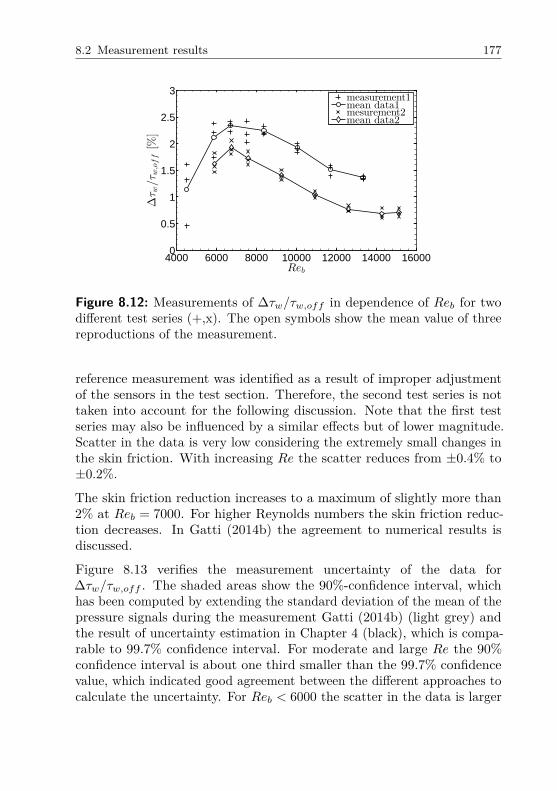
8.2 Measurement results 177
Reb
∆τw/τw,off[%
]
4000 6000 8000 10000 12000 14000 160000
0.5
1
1.5
2
2.5
3measurement1mean data1mesurement2mean data2
Figure 8.12: Measurements of Δ𝜏𝑤/𝜏𝑤,𝑜𝑓𝑓 in dependence of 𝑅𝑒𝑏 for twodifferent test series (+,x). The open symbols show the mean value of threereproductions of the measurement.
reference measurement was identified as a result of improper adjustmentof the sensors in the test section. Therefore, the second test series is nottaken into account for the following discussion. Note that the first testseries may also be influenced by a similar effects but of lower magnitude.Scatter in the data is very low considering the extremely small changes inthe skin friction. With increasing 𝑅𝑒 the scatter reduces from ±0.4% to±0.2%.
The skin friction reduction increases to a maximum of slightly more than2% at 𝑅𝑒𝑏 = 7000. For higher Reynolds numbers the skin friction reduc-tion decreases. In Gatti (2014b) the agreement to numerical results isdiscussed.
Figure 8.13 verifies the measurement uncertainty of the data forΔ𝜏𝑤/𝜏𝑤,𝑜𝑓𝑓 . The shaded areas show the 90%-confidence interval, whichhas been computed by extending the standard deviation of the mean of thepressure signals during the measurement Gatti (2014b) (light grey) andthe result of uncertainty estimation in Chapter 4 (black), which is compa-rable to 99.7% confidence interval. For moderate and large 𝑅𝑒 the 90%confidence interval is about one third smaller than the 99.7% confidencevalue, which indicated good agreement between the different approaches tocalculate the uncertainty. For 𝑅𝑒𝑏 < 6000 the scatter in the data is larger

178 8 Spanwise oscillating walls implemented via dielectric elastomer actuators
Reb
∆τw/τw,off[%
]
4000 6000 8000 10000 12000 14000 160000
0.5
1
1.5
2
2.5
3measurement1mean data1
Figure 8.13: Comparison of the uncertainty in the determination ofΔ𝜏𝑤/𝜏𝑤,𝑜𝑓𝑓 : The measurement data are compared to a 90%-confidenceinterval (light grey) computed in Gatti (2014b) and the result of uncertaintyestimation in Chapter 4 (black).
0 200 400 600 800 1000−1
−0.5
0
0.5
1
Time [s]
(Re b
−Re b)/Re b
[%]
Reb = 5950Reb = 15250
Figure 8.14: Percentage fluctuation of 𝑅𝑒𝑏 around the mean value. For thelower and upper end of the measurement range. The actuator is activatedand deactivated in time intervals of 180s.

8.2 Measurement results 179
Reb
∆C
(r)
f/C
(r)
f,0[%
]
4000 6000 8000 10000 12000 14000 16000−1%
−0.5%
0%
0.5%
1.0%measurement1measurement2
Figure 8.15: Influence of the activation of the DEA on the skin friction onthe upstream reference section. Data for both test series are included. Thegrey shaded area depicts the uncertainty interval according to the analysisin Chapter 4.
than predicted by the present uncertainty calculation. This calculationpredicts an increase of the accuracy due to the switch to the more accuratepressure sensor at the flow meter (compare Chapter 4.2.6). In contrastfor low 𝑅𝑒 the scatter of the data is not dominated by the accuracy ofthe flow meter in this particular measurement. Two other sources leadto an increase of the scatter instead. Firstly, the measurement point at𝑅𝑒𝑏 = 4600 is slightly below 𝑅𝑒𝑏 = 4800, at which a fully turbulent flowcan be ensured throughout both downstream sections of the channel. Thisincreases the scatter in the flow rate, as was found in Chapter 5 and isdepicted in detail in Figure 6.12. Secondly, fluctuations of the flow rateparticularly decrease the measurement accuracy in the DEA testing, sincethe determination of the pressure drop is based only on a small streamwiselength and additionally only one measurement point. The latter aspectwas discussed in Section 8.1.4. It can be concluded that the measurementaccuracy is appropriate for 𝑅𝑒𝑏 > 6000 to identify changes in Δ𝜏𝑤/𝜏𝑤,𝑜𝑓𝑓
in the order of 0.4%. The measurement accuracy increases with the 𝑅𝑒𝑏
and allows to detect changes of 0.2% for 𝑅𝑒𝑏 > 9000.
Figure 8.14 shows the measurements of the flow rate for the completemeasurement time of 18min, in order to prove that the reduced pressureloss along the actuator is not a result of a change in flow rate. The

180 8 Spanwise oscillating walls implemented via dielectric elastomer actuators
actuator is activated and deactivated in time intervals of 180s. Exemplarymeasurements for 𝑅𝑒𝑏 = 5950 and 𝑅𝑒𝑏 = 15250 are depicted, whichrepresent the measurement range in which a high confidence in the resultpreviously was confirmed from the uncertainty quantification. The variationin the flow rate is very small, for the mean value between the three minutesintervals it is far less than 0.1%.
Complementary, Figure 8.15 shows the change in the skin friction on thesmooth reference section Δ𝑐
(𝑟)𝑓 /𝑐
(𝑟)𝑓,0, while the actuator was activated and
deactivated on the simultaneously measured section. On the referencesection the flow is confirmed to be unaffected by the actuation. Scatter inthe data is less than 0.3%, which supports the previously shown result ofthe uncertainty consideration.
8.2.3 DEA in cascaded configuration
For the measurements shown in this paragraph two changes in the set-up were made. The configuration of the actuators has been changed tothe cascaded configuration, Figure 8.8. The main advantage is a longeractuated length in streamwise direction. The second change was the usageof the new WT2 actuator to obtain larger displacement. Unfortunately,the large deformations of the active membrane resulted in more frequentfailures, which reduced the durability of the WT2 actuators.
Since the actuators were only arranged on the upper channel wall, the skinfriction reduction is assumed to double for a virtual two-sided configurationin order to enable comparisons with the first test series:
Δ𝜏𝑤/𝜏𝑤,𝑜𝑓𝑓∼= 2(𝜏𝑤,𝑜𝑓𝑓 − 𝜏𝑤,𝑜𝑛)/𝜏𝑤,𝑜𝑓𝑓 . (8.5)
Gatti (2014b) showed the validity of this approach in a numerical simulationwith the same configuration.
Figure 8.16 shows the results of Δ𝜏𝑤/𝜏𝑤,𝑜𝑓𝑓 for the WT2, which is corre-sponding to the total actuated length. Unfortunately the test series couldnot be completed since the membranes of the actuators broke after fourmeasurements. It can be construed that a even higher Δ𝜏𝑤/𝜏𝑤,𝑜𝑓𝑓 couldhave been achieved at higher 𝑅𝑒. Although only the incomplete data setcan be compared with the WT1 configuration, the measurement indicatea considerable influence of the transient length on the effectiveness of thetechnique.

8.2 Measurement results 181
Reb
∆τw/τw,0[%
]
3000 4000 5000 6000 7000 8000 9000 100000
1
2
3
4
5WT1mean WT1WT2mean WT2
Figure 8.16: Reduction of skin friction for the test of cascaded WT2actuators.
8.2.4 Influence of limited spanwise actuator lengthon skin friction reduction
Analogously to the analysis carried out in Chapter 5.4.3, the drag reductionis corrected by taking into account the deviation of the flat duct from a idealtwo-dimensional flow. Additionally, the fact that only a part of the channelwidth has been actively controlled is also taken into account, assumingthat no drag reduction occurs in the non-actuated surface area. Further-more, the actuation is not homogenous over the complete actuated surface.While the stiffened surface area of the passive membrane (200x200mm forboth actuator types) oscillates homogeneously, the displacement linearlydecreases to zero towards the supporting frames. Therefore, the fraction ofthe actuated length without stiffening is considered with a mean value halfof the maximum displacement. For the WT1 a correction factor for thechange in the skin friction of 𝑘𝑊 𝑇 1=1.4 resulted and for the WT2 type of𝑘𝑊 𝑇 2=1.28. The corrected values for the maximum Δ𝜏𝑤/𝜏𝑤,𝑜𝑓𝑓 are 3.2%for WT1. The WT2 case with cascaded actuators is more complex, sincethe supporting frames between adjacent actuators interrupt the actuatedsurface and cannot be corrected analogously.

182 8 Spanwise oscillating walls implemented via dielectric elastomer actuators
8.3 Discussion of the DEA results
The experiments of the present study were able to proof the applicabilityof the dielectric elastomer actuators for flow control. In reproduciblemeasurements a reduction of the skin friction on the actuated surface wasshown. There are two main reasons for this achievement. On the one hand,the actuators built by Gatti (2014b) were durable and allowed to run awhole experimental campaing with manageable effort; on the other handthe present set-up provided the ideal framework for the actuator testing.In fact, although the reduction was comparably small with maximum threepercent, the accuracy of the instrumentation allowed to precisely investigatethe effect in dependence of 𝑅𝑒. It was shown that for 𝑅𝑒𝑏 > 6000 thechanges in Δ𝜏𝑤/𝜏𝑤,𝑜𝑓𝑓 of the order of 0.4% were statistically significant.The measurement accuracy even increases with the 𝑅𝑒𝑏 and allowed todetect changes of 0.2% for 𝑅𝑒𝑏 > 9000.
The careful measurement of the reference case highlighted an increase of theskin friction on the deactivated actuator in comparison to the reference casefor 𝑅𝑒𝑏 > 7000 (see Fig. 8.11). For 𝑅𝑒𝑏 > 9000 the reduction of 𝜏𝑤 by thewall oscillation does not compensate the increase of the skin friction due tothe presence of the actuator. However, at 𝑅𝑒𝑏 ≈ 6500, where the maximumof Δ𝜏𝑤/𝜏𝑤,𝑜𝑓𝑓 was achieved, there is a holistic drag reduction, meaningthe skin friction is below the value on the smooth reference section.
The DEA developed by Gatti (2014b) can have comparably long life-time.In particular, the WT1 types were still working after more than ten hoursof measurement. The WT1 never showed a defect of the active membrane,but a passive membrane broke twice. The WT2 type turned out to be morefragile. The achievement of large displacement reduced the lifetime of theactive membrane, which impeded a comprehensive study. However, thefew measurement results obtained with the cascaded configuration indicatethat the effectiveness of the spanwise oscillations technique can significantlybe enhanced by increasing the actuated streamwise length.

9 Summary and conclusions
The present work deals with high-precision skin-friction measurements ofvarious active and passive surfaces in a newly built wind-tunnel facility andis comprised of three consecutive parts. The first part contains an in-depthreport of both design and construction of the test-rig. The measurementaccuracy and the precisely adjustable test conditions have been verifiedin the second part by means of a hydraulically smooth reference surface.Subsequently, various passive and active surfaces were tested for their drag-reduction capabilities as compared to this reference. Finally, a discussionof the achieved insights, drawn conclusions and remarks on possible futureefforts with this new test rig closes the present work.
The first part of the work has been devoted to the description of theexperimental facility and its construction, comprising the wind tunnel, thechannel flow test section and the instrumentation. A channel flow testsection with an aspect ratio of 𝐴𝑆 = 12 was chosen to approximate thefavorable test conditions of a two-dimensional flow. The skin friction isdetermined indirectly through measures of the pressure drop in streamwisedirection. A wind tunnel of blower type has been chosen, as it allows tobuilt-up a comparatively high pressure and is compatible to be equippedwith precise flow rate instruments. The modular construction, which allowsthe facility to reliably cover a large operation range and to be highlyextendable, was realized according to the engineer standards DIN ENISO 5167-2 (2003) and DIN 24163 (1985). Air was chosen as the workingmedium in order to allow the application of active flow controllers, some ofwhich cannot operate in liquids. However, this choice implies the demandingtask to measure extremely small variations of small quantities as comparedto measurements in liquids.
Despite this adverse choice of air, it was the main goal of the tunnel andinstrumentation design process to achieve at least comparable accuracyas reported for oil and water tunnels. In particular, the test section hasbeen equipped with pressure transducers of highest accuracy available on

184 9 Summary and conclusions
the market, which made a detection of extremely small pressure variations(thus wall shear stresses) possible. In addition, a precise determinationof the flow rate has been obtained by the use of inlet nozzles and orificemeters. For the latter, parameter range and sensitivity studies have proventhe reproducibility of the measurements and revealed an extended workingrange of nozzle flow meters below their critical flow rate. The detailedestimation of measurement uncertainty and error propagation of preliminarytests identified an insufficient reproducibility (±1%) of the flow rate as themain remaining weakness for the determination of skin friction changes.
To reduce this remaining amount of uncertainty, the resolution of skinfriction changes was further improved by three different approaches duringexperimentation. First, the impact of ambient noise on the measurementdata was identified and these effects on the measurement results wereexcluded. Second, environmental influences like state-variable changeswere minimized by an additional consideration of the varying air humidity.Compensation for this effect further reduced the uncertainty by 0.2%.Third, the experimental procedure has been modified for the respective testcases in so as to ensure highest achievable precision for the comparison ofthe flow controlled surfaces and the reference surfaces. These modificationshave been discussed extensively and their impact on the measurementaccuracy was reflected in the experimental results. In the riblet campaignskin friction changes of 0.4% could be resolved at moderate Reynoldsnumbers of 10000 by a comparison of reference and test surface in twosimultaneously measured sections of the channel. Note that larger Reynoldsnumbers revealed even higher accuracy. In the DEA study the measurementaccuracy of 0.4% was achieved at significantly smaller Reynolds numbersof 6000. For 𝑅𝑒𝑏 > 9000 it even increased to 0.2%. This improvementwas possible, since the actuators were switched on and off repeatedly.Consequently, the relative difference between either case was less affectedby any drift of boundary conditions.
Prior to any flow control experiments, an extensive study of the smoothreference surface was performed, where excellent agreement with literaturewas demonstrated for both laminar and turbulent flow. Furthermore, anaccurate examination of the flow development was possible, which provideda refined specification of the development length of a turbulent channel flow.While in the literature (Durst et al., 1998) for a streamwise distance largerthan 60 channel heights the development was reported to be completed, itturned out from the present study that a streamwise distance of 70 to 80Hshould be exceeded. However, this longer development length implies further

9.1 Comparability of experimental and numerical data 185
skin friction changes of 0.3%, which corresponds to the resolution limit ofwith the present set-up. The resulting overall uncertainty of approximately0.4% proved that wind tunnels can indeed operate as accurate as today’smost accurate oil tunnels (Bechert et al., 1992). Furthermore, to improvethe comparability between experimental studies and numerical simulations,the spanwise distribution of the wall shear stress has been investigated.This data serves as the basis for a correction of the three dimensional effectsgenerated by the channel sidewalls, which will be conclusively discussed inthe next section.
The applicability of the above-introduced test rig for highly accurate skinfriction (reduction) measurements was then demonstrated by means oftwo passive and one active flow control surface. The main emphasis wasplaced on the study of riblet structures and micro grooves. In addition,novel dielectric elastomer actuators (DEA) have been applied in the presenttunnel. The development of the DEA has initially been an independentresearch project (Gatti, 2014b). Since these active flow control actuatorsperfectly fit into the present wind tunnel facility, it was extremely beneficialfor both projects to study the achievable flow control success of DEA inthe present experimental set-up. Insights and drawn conclusions from allthree drag-reduction approaches will be summarized below, as well.
9.1 Comparability of experimentaland numerical data
Already the literature research at the beginning of the work showed thelack of an analytic formulation for the friction coefficient 𝑐𝑓 in a turbulentchannel flow in dependence of 𝑅𝑒. For the experiments where the channelis approximated by a flat duct, the aspect ratio of the width to height ofthe duct 𝐴𝑆 is an additional parameter influencing 𝑐𝑓 . The experimentalapproaches, that are found in literature (Dean, 1978; Johnston, 1973;Zanoun et al., 2009) correlate measurement data for different ranges of𝑅𝑒𝑏. For the calculation of 𝑐𝑓 a uniform spanwise velocity distribution isassumed, which does not consider the presence of the the side walls. Theconsiderable deviation from a two-dimensional flow was confirmed by thecomparison with numerical results (Hoyas & Jimenez, 2008; Iwamoto et al.,2002; Moser et al., 1999). The empirical formulas from all experimentalapproaches were based on the same functional relation to correlate the

186 9 Summary and conclusions
measurement data 𝑐𝑓 = 𝐴 · 𝑅𝑒−0.25𝑏 . In dependence of the considered
𝑅𝑒 range the literature sources found different results for the constant 𝐴,which shows that any of the correlations is not appropriate for a large𝑅𝑒 range. The present data confirmed the approach by Dean (1978) todescribe very accurately the dependence of the skin friction coefficient on𝑅𝑒 for a channel of moderate aspect ratio (𝐴𝑆 = 12) at 𝑅𝑒𝑏 = 4000−24000.These boundary conditions are representative for the most channel flowexperiments for drag reduction investigations of flow control. Although this𝑅𝑒 range contains the low Reynolds numbers at which DNS are conducted,the comparability of the experimental studies to the numerical resultsis decreased due to the different spanwise velocity distribution and theadditional friction generated by the side walls, which affect the obtainedskin friction changes of the flow control applications. To improve thissituation measurements were conducted to quantify the deviation from auniform spanwise wall shear distribution for the present channel. In theconsidered measurement range, the distribution of the wall shear stresswas obtained to be nearly independent of 𝑅𝑒. As a result an empiricalcorrection function for skin friction change 𝛿𝜏𝑤/𝛿𝜏𝑤,0 for an 𝐴𝑆 = 12channel was derived. Assuming the main change of the velocity distributionin dependence of the aspect ratio of flat ducts was the extension of thenearly uniform spanwise distribution, which was found around the channelcenter, the correction function was generalized for channels of 𝐴𝑆 > 5. Amuch better comparability of channel flow experiments of different 𝐴𝑆 andexperimental and numerical data is hypothesized.
9.2 Riblets
The riblet study was the benchmark-test for the experimental set-up,since the riblet structures have been extensively studied (Bechert et al.,1997; Gruneberger & Hage, 2011; Viswanath, 2002; Walsh, 1982; Walsh &Lindemann, 1984; Walsh & Sellers, 1988). In particular the experimentalresearch by Bechert et al. (1997) with a special oil tunnel facility designedfor the detection of skin friction changes is from unmatched quality. It wasdemonstrated that the present set-up very well reproduces these resultsand that scatter in the data of both facilities is comparable, although bothfacilities utilize completely different frameworks for the testing. Bechert’soil tunnel (Bechert et al., 1992) of a rectangular cross section directlymeasures 𝜏𝑤 with a shear stress balance, while the present set-up indirectly

9.3 Microgrooves 187
determines the wall shear stress from the streamwise pressure drop of anairflow. It is the first time that riblets have been measured with suchaccuracy in an air flow.
On that basis it was enabled to exploit the benefit of an air flow facilityto study the flow development on riblet surfaces over long streamwisedistances. After a minimal onset length a constant reduction of the skinfriction on the riblet surface was obtained: The estimate by Walsh (1990)that the amount of drag reduction is independent of the streamwise positionis confirmed.
The study identified the leading edge of the riblets plate to be crucial.Although the investigated structures were very small, the increase of thepressure drop at the leading edge was significant. This observation isin contradiction to Bechert et al. (1997) who found an abrupt begin ofthe riblet structures not to affect the result of 𝜏𝑤/𝜏𝑤,0. Controversialfindings in the literature (Bechert et al., 1997; Squire & Savill, 1986,1987; Walsh, 1990) are indicated to be more related to the design of theexperiment than to the riblets. In wind tunnel facilities the riblet heightis negligible small compared to the dimensions of the facility, while ina channel flow experiment, the protruding riblets are relatively largercompared to characteristic height. Thus, in channel flow experiments,the measurement is much more sensitive to the small blockage by theprotruding fins. Additionally, shear stress balances, which were usuallyused for riblet studies, do not provide a streamwise resolution of the wallshear stress distribution and the comparably small leading edge effect maydisappear within the integral value of the test plate on the balance.
9.3 Microgrooves
Even though disillusioning and contradictory at first glance, the carefulanalysis of the micro groove data reveals clear and conclusive insights. Ithas been demonstrated in the present work that the studies of presuminglyturbulent flow by Frohnapfel et al. (2007a); Jovanovic et al. (2010b) infact were neither turbulent nor fully developed. The different wall shearstress on upstream and downstream section of the channel at low 𝑅𝑒 wasfound to be attributed to the laminar turbulent development of the flow.Hence, the present analysis clearly depicts the strong dependence of the

188 9 Summary and conclusions
significance of measurement results on the measurement uncertainty andthe detailed analysis of the reference case.
For the study in naturally developing flow a modified groove geometrywas chosen. Instead of rectangular, V-shaped grooves were used with theintention to increase the transition delay found by Jovanovic et al. (2011).However, the surfaces with streamwise aligned grooves were not able todelay the transition in the present measurement, but the skin frictionwas equal to that of hydraulically smooth plates. Finally, the reason forthe discrepancies to the measurement of Jovanovic et al. (2011) cannotdefinitely be clarified. Nevertheless, the present study is superior in regardto the measurement accuracy as well as the number and reproducibility ofthe measurements.
Instead the fundamental question arises whether the transition of naturallydeveloping flow in a channel flow facility of this type in generally can bedelayed, if the manipulation is not focusing on the probably dominantfactor to trigger transition: the secondary motions contaminating the walleffects. The present study agrees to this statement by Dean (1978) and isconfirmed by the observations of Arbeiter (2009). Furthermore, the similarReynolds number at which the highest turbulence level was obtained in thepresent study and the investigation by Jovanovic et al. (2011) points in thisdirection. A pipe flow experiment would be beneficial, since a circular crosssection avoids the side wall effects. However, the transition mechanisms ininner flows and a zero pressure gradient boundary layer are not the same.Therefore, contrary to turbulent flows, the results from a pipe flow cannotdirectly be transferred to a boundary layer flow.
The micro grooves idea needs to return to the origin. The misinterpretationof experimental data led to the conclusion (Frohnapfel et al., 2007a), thatthe optimum scaling of the grooves width is in the order of a viscous lengthscale. The theoretical idea as well as the numerical simulations (Frohnapfel,2006) were focusing on dimensions of the viscous sublayer (𝑥+
2 = 5). Theineffectiveness of the grooves probably is not originating from the absenceof one-component turbulence within the groove, but the near wall flow isnot effectively influenced by the grooves. The rectangular groove geometrymust lead to failure, since the interaction of the flow with the sharp angleflanks of the grooves generates a high local friction. Eventual benefitinside the groove is compensated, as was discussed by Walsh (1990) in thecontext of optimization of riblet geometries. The actual groove scalingis so small, that the roughness represented by the structures is negligible

9.4 Dielectric elastomer actuators 189
for a large Reynolds number range. In comparison with the criterion ofNikuradse (1933) the size of micro grooves is diminutive. Also the recentlyidentified effects on turbulent flow by structures of even smaller scalesby Gruneberger & Hage (2011) indicate the micro grooves to be withoutsignificant effect on a turbulent flow. Due to the alignment in flow directionand the surface embedded shape the grooves are of less effect than thesmall fins orientated in cross flow direction in Gruneberger’s investigation(ℎ+ = 0.5). In general, the groove geometry is in contradiction to theriblets design. The experimental investigations by Walsh (1982) showedthat neither V-grooves nor convex semicircular structures, which are verysimilar to the optimized groove geometry suggested in (Frohnapfel, 2006),achieved a reduction of the skin friction drag at a scaling in order of theviscous sublayer and larger.
The idea of the recently investigated similar structures, but of considerablylarger scaling Daschiel (2014) is based on the finding by Eckert & Irvine(1955). Eckert found the co-existence of laminar and turbulent flow inpipes of non-circular cross sections, which were suggested for a transitiondelay in Eckert & Irvine (1960). This approach is adapted in Daschiel(2014) where the scaling of the grooves is not of the order of typical surfacemorphology, but represents a modification of the global shape of the crosssection. From the view point of the present author, the development oftheses large-scale structures for transition delay is the only remainingstarting-point to achieve a drag reduction on base of the idea of streamwisealigned groove structures.
9.4 Dielectric elastomer actuators
In the DEA study the implementation of an active flow control techniqueinto the channel test section has been successfully demonstrated. Thesenovel actuator type to generate an oscillating wall is quite fragile andconductivity of the working fluid is problematic. Therefore, to studyactuators of such type is only possible in an air flow experiment. The shortstreamwise length of the actuated surface represented a very challengingaspect in testing the DEA. The most effective operation of the actuatorsis found in the 𝑅𝑒 range of 4000 < 𝑅𝑒𝑏 < 8000, in which the pressuredrop along such a small streamwise distance (200mm) was between 0.6Paand 2Pa. The changes due to the actuation were even two orders less.
190 9 Summary and conclusions
Despite these challenging aspects the measurement strategy, which enabledto compare the deactivated and activated devices alternating, turned outbeneficial for the significance of the measurement with the active device.The experimental set-up verified the calculated uncertainty to allow thedetection of changes in the skin-friction with an accuracy of 0.4% at𝑅𝑒𝑏 = 6000. The significance even increased with 𝑅𝑒𝑏 and allowed todetect changes of 0.2% for 𝑅𝑒𝑏 > 9000, which demonstrates the maximumaccuracy to be almost independent of the considered streamwise distance.
With the dielectric elastomer actuators a reduction of the friction aboutΔ𝜏𝑤,𝑚𝑎𝑥 = 3% has been precisely quantified. It was also shown that theskin friction was reduced below the value of a simultaneously measuredhydraulically smooth surface, on which the skin friction very well agreedto the correlation by Dean (1978).
The actuators developed by Gatti (2014b) represent substantial progress.In contrast to the dielectric elastomer based actuators shown by Gouderet al. (2013), who reported the life-time of the devices to be few minutes,Gatti’s WT1 actuators sustained ten hours of testing without damage.Through the insufficient durability of the WT2 actuators this test serieswas interrupted and remained incomplete. However, in preliminary testingto check the proper working of the set-up with actuators, significantlylarger drag reduction has been observed. It is not adventurous to predictthat this technique can have twice the effectiveness than what could berecorded in the present study.

10 Outlook
The first part of the outlook aims to expose the variability of the presentset-up to inspire future research projects using the facility. The secondpart suggests practical examples to continue research related to the presentstudy.
10.1 Prospects of the facility
The following section discusses further improvement of the facility andhighlights the potentials of the large operative range and variability of thefacility in different configurations.
With regard to the absolute accuracy of the skin friction determination acalibration of the orifice meters would be desirable. While the detectionof changes in 𝜏𝑤/𝜏𝑤,0 is of very high accuracy, the uncertainty of the skinfriction detection could be further improved. In Chapter 4 it was elaborated,that the largest contribution to the uncertainty of the determination ofthe skin friction originates from the flow rate meter. The systematicuncertainty of the flow coefficient of the orifice meter was identified to beabout half of the total uncertainty of the flow rate measurement. Notethat the agreement to Dean’s law implies that there is an uncertainty inthe flow coefficient, but the effectively resulting error is very small. Animprovement of the accuracy of flow meters can be achieved by a calibrationusing an instrument, for instance an inlet nozzle, of high specified accuracy.The required test rig for a direct comparison of different flow rate metersthrough simultaneous measurement has already been tested during thepresent work (see Appendix A.1).
If future projects continue to use the wind tunnel configuration with thechannel test section of the present work, it might be useful to install asmaller blower with maximum flow rate about 2500m3/h and the maximumpressure built-up at lower flow rates. This would be advantageous to

192 10 Outlook
achieve even more constant flow rates at very low 𝑅𝑒. Additionally theminimum flow rate could be reduced to 𝑅𝑒𝑏 ≈ 1500, which would enlargethe operation range in laminar flow. The flow rate instrumentation wouldonly require a smaller orifice disk to be adapted to the new operationrange.
In order to attend to the recent numerical results by Daschiel (2014), itwould be straight-forward to combine the wind tunnel with a pipe flowtest section. The enormous length (18m) of the laboratory in Karlsruherepresents perfect boundary conditions to use the facility in combinationwith a long pipe test section. This pipe test section would also takeadvantage of all previously mentioned suggestions for improvement of theexperimental set-up.
One potential option is to build a test section of comparably large crosssection in the range of 0.5m× 0.3m (𝑊 × 𝐻) to generate a wind tunneldesign like a “pressure driven Eiffel tunnel”. Since this type of tunnel islacking at the institute in Karlsruhe. It might be even useful to equipthe facility with a larger ventilator for this purpose. The Eiffel tunnelconfiguration would allow to conduct experiments for classical aerodynamicresearch.
10.2 Studies of channel flow
In order to improve the comparability of numerical and experimentalstudies of channel flow an empirical approach based on measurementsof the spanwise distribution of the velocity and the wall shear stress forturbulent flow was made. However, in the experimental investigationsit is not possible to study the ideal two-dimensional reference case andthus we cannot compare experiment results of the approach by the flatduct with the uniform velocity distribution. In the numerical studiesthis would be possible. The two-dimensional channel flow with periodicboundary conditions has been intensively studied (Hoyas & Jimenez, 2008;Iwamoto et al., 2002; Moser et al., 1999). Additionally, numerical studiesallow to investigate the flow in a flat duct and to study the influenceof secondary flows, which was not possible in the present experimentalapproach. Recently, numerical studies by Vinuesa (2013) and Vinuesa et al.(2014) showed results for flat ducts including such data. However, the 𝑅𝑒was quite low and the aspect ratio was limited to 𝐴𝑆 = 7, which is still too

10.2 Studies of channel flow 193
low to approximate a two-dimensional flow. It would be worth to invest thetime for DNS at moderate Reynolds numbers of 5000 to 6000 of duct flowswith 𝐴𝑆 ≥ 10 for a direct comparison with the two-dimensional results.This would allow to verify and refine the experimental approach of thepresent study. The outcome would be meaningful for any channel flowexperiment both numerical and experimental.
The essential question which came along with the studies of naturallydeveloping channel flow is the releasing mechanism of the transition toturbulence in a flat duct. The literature could not answer the question towhich degree the sidewall effects contaminate the cross section. Neithera specification of the streamwise length, nor the 𝑅𝑒 range, where theseeffects begin to dominate the transition process is given. An essentialquestion is whether an higher aspect ratio would limit the contaminationof the flow by the sidewall effects to a distinct area and the channel centerwould remain unaffected. This is indicated in measurements by Nishioka &Masahito (1984), where a channel with a large aspect ratio of 27.4 was used.Although the tunnel is quite long, 𝐿/𝐻 = 400, laminar flow is retained upto 𝑅𝑒𝑏 = 10650. The contamination of the flow by vortices originating fromthe sidewalls is not mentioned there. However, only the 60% around thecenter of spanwise velocity distribution is shown by Nishioka et al. (1975)and the sidewall region is omitted. It is speculated that this spanwise areais mainly influenced by the sidewall effects. Anyhow, this large aspect ratiochannel exhibits a region in the channel center, which is not affected bythe secondary flows. It can be deduced that the aspect ratio may play amore important role for transition process than initially considered.
To study the development of the corner vortices, the available channelcould be equipped with plexiglas plates on top. Additionally, a seedinggenerator at the entrance of the nozzle for a flow visualization would berequired. This would allow to study the occurrence and development ofthe contamination of the spanwise flow field in dependence of 𝑅𝑒 and therunning length. Eventually, the present channel would be more convenientfor transition testing in a shortened configuration, where the sidewall effectshave less streamwise distance to develop.

194 10 Outlook
10.3 Channel flow studies at high Re
The experimental set-up allows to operate the channel test section atsignificantly higher 𝑅𝑒. With the available diffuser at the outlet of thechannel 𝑅𝑒𝑏 > 40000 has been achieved. If the suggestion to install ablower with larger pressure built-up is followed, the Reynolds number canbe increased to more than twice this value. In the following two ideas,which are based on this high 𝑅𝑒 configuration, are described to contributeto quite fundamental questions.
Recently Gatti (2014b) discussed the decrease in drag reduction effectivenessof flow control techniques with increasing Reynolds number, which has beenobtained in numerical as well as experimental studies. The experimentdescribed in the following could contribute to verify the relation of the dragreduction on 𝑅𝑒, which was proposed by Gatti (2014b).
From the present riblet study it can be observed that an accuracy ofdetermining skin frictions changes of 0.4% would be ensured for 𝑅𝑒𝑏 ≥10000. If two similar riblet structures at different scaling could be produced,with an optimum spacing about 𝑅𝑒𝑏 = 10000 and 𝑅𝑒𝑏 = 80000 the effect ofthe Reynolds number on the drag reduction could be studied very precisely.Note that it would not be required to produce high performance riblets, butto achieve the same relative fabrication quality of both riblet surfaces.
Additionally, the high 𝑅𝑒 set-up would allow to investigate the skin frictioncoefficient for a wide Reynolds number range with an accuracy, which hasnot been achieved before. It would enable to study the change of the skinfriction coefficient at higher Reynolds number. Thereby one important issueneeds to be considered: the change in the spanwise velocity profile withincreasing 𝑅𝑒, which was indicated in Chapter 5.4. The function previouslyused (Dean, 1978; Johnston, 1973; Zanoun et al., 2009) 𝑐𝑓 = 𝐴 · 𝑅𝑒−0.25
was found to be unsuitable to describe the dependence of 𝑐𝑓 on wide rangeof 𝑅𝑒. Instead even 𝐴 is supposed to depend on 𝑅𝑒.
The gain would be an accurate empirical correlation for 𝑐𝑓 = 𝑓(𝑅𝑒𝑏) fora channel with an aspect ratio of 12. In optimal case the outcome couldbe combined with result of the previously suggested study to quantifythe difference of numerical and experimental channel flows to achieve acorrelation for 𝑐𝑓 = 𝑓(𝑅𝑒𝑏, 𝐴𝑆).

Bibliography
Arbeiter, F. 2009. Untersuchungen von Kuhlgasstromungen bei transi-tionellen Reynoldszahlen im Einlaufbereich von Minikanalen. Ph.D.thesis, Universitat Karlsruhe.
Arbeiter, F., Gordeev, S., Heinzel, V., Ihli, T., Leichtle, D., Möslang, A.,& Slobotchouka, V. 2008. Features and optimization approaches of theentrance section cooling gas flow of IFMIF High Flux Module. FusionEngineering and Design, 83, 1536–1542.
Bailey, S. C. C., Hultmark, M., Monty, J. P., Alfredsson, P. H., Chong,M. S., Duncan, R. D., Fransson, J. H. M., Hutchins, N., Marusic, I.,McKeon, B. J., Nagib, H. M., Orlu, R., Segalini, A., Smits, A. J., &Vinuesa, R. 5. 2013. Obtaining accurate mean velocity measurements inhigh Reynolds number turbulent boundary layers using Pitot tubes. J.Fluid Mech., 715, 642–670.
Baron, A., & Quadrio, M. 1996. Turbulent drag reduction by spanwisewall oscillations. Appl. Sci. Res., 55, 311–326.
Bechert, D. W. 1995. Calibration of Preston tube. AIAA Journal, 34(1),205–206.
Bechert, D. W, Hoppe, G., van der Hoeven, J. G. T., & Makris, R. 1992.The Berlin oil channel for drag reduction research. Exp. Fluids, 12,251–260.
Bechert, D.W. 1988. Some concepts and facilities for drag reductionresearch. Third Turbulent Drag Reduction Working Party, ONERA-Chatilion, Paris.
Bechert, D.W., & Bartenwerfer, M. 1989. The viscous flow on surfaceswith longitudinal ribs. J. Fluid Mech., 206, 105–209.
Bechert, D.W., Bruse, M., Hage, W., van der Hoeven, J.G.T., & Hoppe,G. 1997. Experiments on drag-reducing surfaces and their optimizationwith an adjustable geometry. J. Fluid Mech., 338, 59–87.

196 Bibliography
Blasius, H. 1913. Das Ahnlichkeitsgesetz bei Reibungsvorgängen in Flüs-sigkeiten. Forsch.-Arb. Ing.-Wes., Heft 131.
Bradshaw, P. 2000. A note on “critical roughness height” and “transitionalroughness”. Phys. Fluids, 12(6), 1611–1614.
Bradshaw, P., & Pankhurst, R. C. 1964. The design of low speed windtunnels. Progr. Aeronaut. Sciences, 5, 1–69.
Bradshaw, Peter, Gregory, Nigel, & Britain, Great. 1961. The determinationof local turbulent skin friction from observations in the viscous sub-layer.HM Stationery Office.
Byrne, J., Hatton, A.P., & Marriot, P.G. 1970. Turbulent flow and heattransfer in the entrance region of a parallel wall passage. Proc. Instn.Mech. Engrs., 184(39), 697–710.
Carlson, D. R., Widnall, S. E., & Peeters, M. F. 1982. A flow visualizationstudy of transition in plane Poiseuille flow. J. Fluid Mech., 121, 487–505.
Cattafesta, Louis N., & Sheplak, Mark. 2011. Actuators for active flowcontrol. Ann. Rev. Fluid Mech., 43, 247–272.
Choi, H., Moin, P., & Kim, J. 1991. On the effect of riblets in fullydeveloped laminar channel flows. Phys. Fluids, A3(1892).
Choi, H., Moin, P., & Kim, J. 1993. Direct numerical simulation of turbulentflow over riblets. J. Fluid Mech., 255, 503–539.
Choi, J.-I., Xu, C.-X., & Sung, H. J. 2002. Drag reduction by spanwise walloscillation in wall-bounded turbulent flows. AIAA J., 40(5), 842–850.
Choi, K.-S., & Clayton, B.R. 2001. The mechanism of turbulent dragreduction with wall oscillation. Int. J. Heat a. Fluid Flow, 22, 1–9.
Choi, K-S., DeBisschop, J.R., & Clayton, B.R. 1998. Turbulent boundary-layer control by means of spanwise-wall oscillation. AIAA J., 36(7),1157–1162.
Colebrook, C.F. 1939. Turbulent flows in pipes with particular reference tothe transition between the smooth- and rough-pipe laws. J. Inst. CivilEng., 11, 133–156.
Coleman, H. W., & Steele, W. G. 2009. Experimentation, validation, anduncertainty analysis for engineers. John Wiley & Sons, Inc.

Bibliography 197
Czichos, H., & Hennecke, M. 2004. Hütte, Das Ingenieurswesen 32. Auflage.Springer.
Daschiel, G. 2014. Strategies to reduce friction losses and their implicationsfor the energy efficient design of internal flow domains. Ph.D. thesis,Karlsruher Institut fur Technologie.
Davies, S. J., & White, C. M. 1928. An experimental study of the flow ofwater pipes of rectangular section. Proc. R. Soc. London A, 119, 92–107.
Dean, B, & Bhushan, B. 2010. Shark-skin surfaces for fluid-drag reductionin turbulent flow: a review. Phil. Trans. R. Soc. A, 368, 4775–4806.
Dean, R. B. 1978. Reynolds number dependence of skin friction and otherbulk flow variables in two-dimensional rectangular duct flow. J. FluidsEngin., 100, 215–223.
Di Cicca, G.M., Iuso, G., Spazzini, P.G., & Onorato, M. 2002. PIVinvestigation of turbulent boundary layer manipulated by spanwise walloscillations. J. Fluid Mech., 467, 41–56.
DIN 24163. 1985. Ventilatoren. German Standard.
DIN EN ISO 5167-1. 2003. Durchflussmessung von Fluiden mit Drossel-geraten in voll durchstromten Leitungen mit Kreisquerschnitt - Allge-meine Grundlagen und Anforderungen. International Standard (Germanversion).
DIN EN ISO 5167-2. 2003. Durchflussmessung von Fluiden mit Drossel-geraten in voll durchstromten Leitungen mit Kreisquerschnitt - Blenden.International Standard (German version).
Duchmann, A., Grundmann, S., & Tropea, C. 2013. Delay of naturaltransition with dielectric barrier discharges. Exp. Fluids, 54, 1461.
Duque-Daza, C.A., Baig, M.F., Lockerby, D.A., Chernyshenko, S.I., &Davies, C. 2012. Modelling turbulent skin-friction control using linearisedNavier-Stokes equations. J. Fluid Mech., 702, 403–414.
Durst, F., Fischer, M., Jovanovic, J., & Kikura, H. 1998. Method to set upand investigate low Reynolds number, fully developed turbulent planechannel flows. Trans. ASME I: J. Fluids Eng., 120(3), 496–503.
Durst, F., Ray, S., Unsal, B., & Bayoumi, O. A. 2005. The developmentlength of laminar pipe and channel flows. Trans. ASME, 127(6), 1154–1160.
198 Bibliography
Eckert, E. R. G., & Irvine, T. F. 1955. Simultaneous turbulent and laminarflow in ducts with noncircular cross section. J. Aeronaut. Sciences, 22,65.
Eckert, E. R. G., & Irvine, T. F. 1960. Laminar skin friction and heattransfer on flat plates with wedge-shaped grooves in flow direction. Trans.ASME, 82(4), 325–332.
Eggels, J.G.M., Unger, F., Weiss, M.H., Westerweel, J., Adrian, R.J.,Fiedrich, R., & Nieuwstadt, F.T.M. 1994. Fully developed turbulent pipeflow: a comparison between direct numerical simulation and experiment.J. Fluid Mech., 268, 175–209.
Ferriss, DH. 1965. Preston tube measurements in turbulent boundary layersand fully developed pipe flow. HM Stationery Office.
Fink, V. 2014. Numerical investigation of the impact of riblets on turbulentchannel flow. Master’s thesis, Karlruher Institut fur Technologie.
Frohnapfel, B. 2006. Flow control of near-wall turbulence. Ph.D. thesis,Universitat Erlangen-Nurnberg.
Frohnapfel, B., Jovanovic, J., & Delgado, A. 2007a. Experimental inves-tigations of turbulent drag reduction by surface-embedded grooves. J.Fluid Mech., 590, 107–116.
Frohnapfel, B., Lammers, P., Jovanovic, J., & Durst, F. 2007b. Interpreta-tion of the mechanism associated with turbulent drag reduction in termsof anisotropy invariants. J. Fluid Mech,, 577, 457–466.
Frohnapfel, B., Lammers, P., & Jovanovic, J. 2007c. New results innumerical and experimental fluid mechanics. Springer. Chap. The roleof turbulent disspation for flow control of near-wall turbulence, pages268–275.
Frohnapfel, B, Lammers, P., Jovanovic, J., & Delgado, A. 2008. Hydraulicmodel of the skin friction reduction with surface grooves. IUTAMSymposium on Flow Control and MEMS, 7, 427–431.
Fulachier, L., Djenidi, L., & Anselmet, F. 1987. Boundary layers on longi-tudinally grooves “Riblets”. Association Aeronautique at Astronautiquede France, PB 88(205620).
Gad-el Hak, M. 2000. Flow control – passive, active and reactive FlowManagement. Cambridge University Press.

Bibliography 199
Gallagher, J. A., & Thomas, A. S. W. 1984. Turbulent boundary layercharacteristics over streamwise grooves. AIAA Paper 84-2185.
Garcia-Mayoral, R., & Jimenez, J. 2011. Hydrodynamic stability and thebreakdown of the viscous regime over riblets. J. Fluid. Mech., 678,317–347.
Gatti, D. 2014a. Mean velocity profile of turbulent channel flows at 𝑅𝑒𝐵 =13650. Tech. rept. Technische Universitat Darmstadt.
Gatti, D. 2014b. Turbulent skin-friction drag reduction via spanwise walloscillations. Ph.D. thesis, Technischen Universitat Darmstadt.
Gatti, D., & Quadrio, M. 2013. Performance losses of drag-reducingspanwise forcing at moderate values of the Reynolds number. Phys.Fluids, 25(125109).
Gatti, D., Haus, H., Matysek, M., Frohnapfel, B., Tropea, C., & Schlaak,H. F. 2014. The dielectric breakdown limit of silicone dielectric elastomeractuators. Appl. Phys. Lett., 104(5), 052905.
Gouder, K. 2011. Turbulent friction drag reduction using electroactivepolymer surfaces. Ph.D. thesis, Imperical College, London.
Gouder, K., Potter, M., & Morrison, J.F. 2013. Turbulent friction dragreduction using electroactive polymer and electromagnetically drivensurfaces. Exp. Fluids, 54(1), 1441.
Gruneberger, R., & Hage, W. 2011. Drag characteristics of longitudinaland transverse riblets at low dimensionless spacings. Exp. Fluids, 50(2),363–373.
Hartnett, J. P., Koh, J. C. Y., & McComas, S. T. 1962. A comparisonof predicted and measured friction factors for turbulent flow throughrectangular ducts. ASME J. Heat Trans., 84, 82–88.
Head, M. R., & Rechenberg, I. 1962. The Preston tube as a means ofmeasuring skin friction. J. Fluid Mech., 14, 1–17.
Herwig, H., & Voigt, M. 1995. Turbulent entrance flow in a channel: Anasymptotic approach. Lecture Notes in Physics, 442(51-58).
Herwig, Heinz. 2008. Stromungsmechanik. Vieweg+Teubner Verlag.

200 Bibliography
Hoagland, L. C. 1960. Fully developed turbulent channel flow in straightrectangular ducts - secondray flow, its cause and effct on the primaryflow. Ph.D. thesis, Massachusetts Institute of Technology.
Holderried, S. 2011. Inbetriebnahme des neuen Windkanals “Emmy”. Bach-elor’s thesis, Technische Universitat Darmstadt.
Hoyas, S., & Jimenez, J. 2008. Reynolds number effects on the Reynolds-stress budgets in turbulent channels. Phys. Fluids, 20(10), 101511.
Huebscher, R. G. 1947. Friction in round, square and rectangular ducts.Heating, Piping and Air Conditioning, 19, 455–467.
Iwamoto, K., Suzuki, Y., & Kasagi, N. 2002. Reynolds number effect onwall turbulence: toward effective feedback control. Int. J. Heat FluidFlow, 23(5), 678–689.
Jimenez, J., Hoyas, S., Simens, M. P., & Mizuno, Y. 2010. Turbulentboundary layers and channels at moderate Reynolds numbers. J. FluidMech.
Johnston, J. P. 1973. The suppression of shear layer turbulence in rotatingsystems. ASME J. Fluids Engin., 95(229-236).
Jovanovic, J. 2004. The statistical dynamics of turbulence. Springer.
Jovanovic, J., Frohnapfel, B, Lienhart, H., & Delgado, A. 2010a. Experi-mental investigation of viscous drag reduction by flow control of laminarto turbulent transition using microgroove surface pattern. ETMM8,Marseille, France, 773–780.
Jovanovic, J., Frohnapfel, B., & Delgado, A. 2010b. Viscous drag reductionwith surface-embedded grooves. Turbulence and interactions, notes onnumerical fluid mechanics and multidisciplinary design, 110, 191–197.
Jovanovic, J., Frohnapfel, B., Srikantharajah, R., Jovanoviťc, D., Lienhart,H., & Delgado, A. 2011. Microflow-based control of near-wall fluctuationsfor large viscous drag reduction. Microfluid Nanofluid, 11, 773–780.
Jung, W.J., Mangiavacchi, N., & Akhavan, R. 1992. Suppression of tur-bulence in wall-bounded flows by high-frequency spanwise oscillations.Phys. Fluids A, 4 (8), 1605–1607.
Kennedy, J. F., Hsu, S.-T., & Liu, J.-T. 1973. Turbulent flows pastboundaries with small streamwise fins. J. Fluid Mech., 99, 605–616.

Bibliography 201
Kim, J., Moin, P., & Moser, R. 1987. Turbulence statistics in fully developedchannel flow at low Reynolds number. J. Fluid Mech., 177, 133–166.
King, R. A., & Breuer, K. S. 2001. Acoustic receptivity and evolution oftwo-dimensional and oblique disturbances in a Blasius boundary layer.J. Fluid Mech., 432, 69–90.
King, R. A., & Breuer, K. S. 2002. Oblique transition in a laminar Blasiusboundary layer. J. Fluid Mech., 453, 177–200.
Kline, S. J., Reynolds, W. C., Schraub, F. A., & Runstadler, P. W. 1967.The structure of turbulent boundary layers. J. Fluid Mech., 30, 741–773.
Kurz, A., Goldin, N., King, R., Tropea, C., & Grundmann, S. 2013. Hybridtransition control approach for plasma actuators. Exp. Fluids, 54(11),1–4.
Lammers, P., Jovanovic, J., & Durst, F. 2006. Numerical experimentson wall turbulence at low Reynolds number. J. Therm. Science, 10(2),33–62.
Laufer, J. 1951. Investigation of turbulent flow in a two-dimensional channel.NACA Rept. 1053.
Lee, S.-J., & Choi, Y.-S. 2008. Decrement of spanwise vortices by adrag-reducing riblet surface. J. Turb., 9(23), 1–15.
Lee, S.-J., & Lee, S.-H. 2001. Flow field analysis of a turbulent boundarylayer over a riblet surface. Exp. Fluids, 30, 153–166.
Liandrat, J. 1988. Laminar boundary layer over riblets. A first step towardsthe turbulent case. Third Turbulent Drag Reduction Working Party,ONERA-Chatilion, Paris.
Luchini, P. 1993. Viscous sublayer analysis of riblets and wire arrays. Appl.Sci. Res., 50, 255–266.
Luchini, P., & Quadrio, M. 2006. A low-cost parallel implementation ofdirect numerical simulation of wall turbulence. J. Comp. Phys., 211(2),551–571.
Luchini, P., Manzo, F., & Pozzi, A. 1991. Resistance of a grooved surfaceto parallel flow and cross-flow. J. Fluid Mech., 228, 87–109.
Lumley, J. 1977. Drag reduction in two-phase and polymer flows. Phys.Fluids, 20(10), 64.

202 Bibliography
Lumley, J., & Kobu, I. 1985. Turbulent drag reduction by polymer additives:a survey. In: B. Gampert – Springer Verlag (ed), The influence of polymeradditives on velocity and temperature fields (IUTAM symposium Essen1984).
Marusic, I., McKeon, B. J., Monkewitz, P. A., Nagib, H. M., Smits, A. J., &R., Sreenivasan K. 2010. Wall-bounded turbulent flows at high Reynoldsnumbers: Recent advances and key issues. Phys. Fluids, 22.
McKeon, B. J., Li, J., Jiang, W., Morrison, J. F., & Smits, A. J. 1999.Further observations on the mean velocity distribution in fully developedpipe flow. J. Fluid Mech., 501(135).
McKeon, B. J., Li, J., Jiang, W., Morrison, J. F., & Smits, A. J. 2003.Pitot probe corrections in fully developed turbulent pipe flow. Meas. Sci.Tech., 14, 1449–1458.
McLean, J., George-Falvy, D., & Sullivan, P. 1987. Flight test of turbulentskin-friction reduction by riblets. Pages 408–424 of: Proc. RAeS Int.Conf. on Turbulent Drag Reduction by Passive Means, London, vol. RAeS2. Royal Aeronautical Society.
Mehta, R.D., & Bradshaw, P. 1979. Design rules for small low-speed windtunnels. Aero. J., 73, 443.
Moin, P., & Mahesh, K. 1998. DIRECT NUMERICAL SIMULATION: Atool in turbulence research. Ann. Rev. Fluid Mech., 30, 539–578.
Monty, J. P. 2005. Developments in smooth wall turbulent duct flows. Ph.D.thesis, The University of Melbourne.
Moody, L. F., & Princeton, N. J. 1944. Friction factors for pipe flow. Trans.ASME, 66(8), 671–684.
Moreau, E. 2007. Airflow control by non-thermal plasma actuators. J.Phys. D: Appl. Phys., 40, 605–636.
Moser, R. D., Kim, J., & Mansour, N. N. 1999. Direct numerical simulationof turbulent channel flow up to Re= 590. Phys. Fluids, 11(4), 943–945.
Nagib, H. M., Vinuesa, R., Noorani, A., Lozano-Duran, a., El Khoury, G.,Schlatter, P., & Fischer, P. F. 2013. Direct numerical simulations ofvariable-aspect-ratio turbulent duct flows at low to moderate Reynoldsnumbers. presented at the TSFP8 in Poitiers, France.

Bibliography 203
Nikuradse, J. 1932. Gesetzmaßigkeiten der turbulenten Strömung in glattenRohren. Forschungsheft 356, Beilage zu Forschung auf dem Gebiete desIngenieurwesens, Ausgabe B Band 3, VDI-Verlag Berlin.
Nikuradse, J. 1933. Stromungsgesteze in Rauhen Rohren. VDI Forsch. 361.(Engl. Trans. 1950. Laws of flow in rough pipes. NACA TM 1292).
Nishioka, M., Iida, S., & Ichikawa, Y. 1975. An experimental investigationof the stability of a plane Poiseuille flow. J. Fluid Mech., 72, 731–751.
Nishioka, M., M., & Masahito, A. 1984. Some observations of the subcriticaltransition in plane Poiseuille flow. J. Fluid Mech., 150, 441–450.
Nitsche, W., & Brunn, A. 2006. Strömungsmesstechnik. Springer.
Orszag, S. A., & Patera, A. T. 1983. Secondary instability of wall-boundedshear flows. J. Fluid Mech,, 38, 347–385.
Patel, V. C. 1965. Calibration of the Preston tube and limitations on itsuse in Pressure Gradients. J. Fluid Mech., 23, 185–208.
Pope, A., & Harper, J.J. 1966. Low-speed wind tunnel testing. John Wiley& Sons, Inc.
Pope, S.B. 2000. Turbulent Flows. Cambridge University Press, Cambridge.
Preston, J.H. 1954. The determination of turbulent skin friction by meansof Pitot tubes. J. R. Aeronaut Soc., 14, 109–121.
Quadrio, M., & Ricco, P. 2003. Initial response of a turbulent channel flowto spanwise oscillation of the walls. J. Turb., 4(7).
Quadrio, M., & Ricco, P. 2004. Critical assessment of turbulent dragreduction through spanwise wall oscillation. J. Fluid Mech., 521, 251–271.
Quadrio, M., & Sibilla, S. 2000. Numerical simulation of turbulent flow ina pipe oscillating around its axis. J. Fluid Mech., 424, 217–241.
Reader-Harris, M. J., & Sattary, J. a. 1996. The orifice plate dischargecoefficient equation - the equation for ISO 5167-1. In Proc. of 14thNorth Sea Flow Measurement Workshop, Peebles, Scotland, East Kilbride,Glasgow, National Engineering Laboratory.
Reif, W.-E. 1978. Protective and hydrodynamic function of the dermalskeleton of elamolranshs. Neues Jahrbuch fur Geologie und Paleontologie,157, 133–141.

204 Bibliography
Reif, W.-E., & Dinkelacker, A. 1982. Hydrodynamics of the squamation infast swimming sharks. Neues Jahrbuch fur Geologie und Paleontologie,164, 184–187.
Reynolds, O. 1883. An experimental investigation of the circumstanceswhich determine whether the motion of water shall be direct or sinuous,and of the law of resistance in parallel channels. Phil. Trans. R. Soc. A,174, 935–982.
Ricco, P., & Quadrio, M. 2008. Wall-oscillation conditions for drag reductionin turbulent channel flow. Int. J. Heat Fluid Flow, 29, 601–612.
Ricco, P., & Wu, S. 2004. On the effects of lateral wall oscillations on aturbulent boundary layer. Exp. Therm. Fluid Sci., 29(1), 41–52.
Sareen, A., Deters, R. W., Henry, S. P., & Selig, M. S. 2011. Drag reductionusing riblet film applied to airfoils for wind turbines. AIAA Paper 2011-588, 588.
Savill, A. M. 1986. Effects of turbulent boundary bayer structure oflongitudinal riblets alone and in combination with outer layer devides.Fourth International Symposium on Flow Visualization, Paris.
Sawyer, W. G., & Winter, K. G. 1987. An investigation of the effect onturbulent skin friction of surfaces with streamwise grooves. TurbulentDrag Reduction by Passive means Conference, London.
Schickel, T. 2012. Beeinflussung einer Kanalströmung durch mikrostrukturi-erte Oberflächen. Bachelor’s thesis, Technische Universitat Darmstadt.
Schlichting, H. 1934. Laminare Kanaleinlaufströmung. ZAMM, 13, 260–263.
Schlichting, H. 1959. Grenzschichtheorie. G. Braun, Karlsruhe.
Schlichting, H., & Gersten, K. 2000. Boundary-layer theory. Springer,Berlin.
Schultz, M. P., & Flack, K. A. 2013. Reynolds-number scaling of turbulentchannel flow. Phys. Fluids, 25.
Skinner, G. T:. 1951. Mean speed measurements in two-dimensional, incom-pressible, fully-developed turbulent channel flow. M.Phil. thesis, CaliforniaInstitut of Technology.
Spiegel, E. A. 2013. Laminare Strömungskontrolle durch in die Oberflächeeingebettete Rillen. Master’s thesis, Universität Erlangen-Nürnberg.

Bibliography 205
Spudat, W. 1981. Erstellung einer Dokumentation uber den Mehrzweck-versuchsstand MZV des Lehrstuhls für Stromungslehre. Studienarbeit,Universitat Erlangen-Nurnberg.
Spurk, H., & Aksel, N. 2006. Stromungslehre. Springer.
Squire, L. C., & Savill, A. M. 1986. High-speed riblets. European Meetingon Turbulent Drag Reduction, Lausanne.
Squire, L. C., & Savill, A. M. 1987. Some experiences of riblets at transonicspeeds. Turbulent Drag Reduction by Passive Means Conference, London.
Stokes, G. 1851. On the effect of the internal friction of fluids on the motionof pendulums. Trans. Cambridge Phil. Soc., 9, 8–106.
Sutardi, & Ching, C. Y. 2001. Effect of tube diameter on Preston tubecalibration curves for the measurement wall shear stess. Exp. Therm.Fluid Science, 24, 93–97.
Toms, B. A. 1948. Some observations on the flow of linear polymer solutionsthrough straight tubes at large Reynolds numbers. Proc. Int. Congr. onRheology, North-Holland, Amsterdam, 2, 135–141.
Touber, E., & Leschziner, M.A. 2012. Near-wall streak modification byspanwise oscillatory wall motion and drag-reduction mechanisms. J.Fluid Mech., 693, 150–200.
Tropea, C., Damaschke, N., & Nobach, H. 2003. Grundlagen der Messtech-nik I. Shaker Verlag.
Tropea, C., Yarin, A., & Foss, J. F. (eds). 2007. Handbook of ExperimentalFluid Mechanics. Springer.
Trujillo, S.M., Bogard, D.G., & Ball, K.S. 1997. Turbulent boundary layerdrag reduction using an oscillating wall. AIAA Paper 97-1870.
VDI. 2002. VDI-Warmeatlas. Springer-Verlag.
Vinuesa, R. 2013. Synergetic computational and experimental studies ofwall-bounded turbulent flows and their two-dimensionality. Ph.D. thesis,Illinois Institute of Technology.
Vinuesa, R., Noorani, A. N., Lozano-Duran, A., El Khoury, G.E.K., Schlat-ter, P.and Fischer, P F, & Nagib, H.M. 2014. Aspect ratio effects inturbulent duct flows studied through direct numerical simulation. J.Turb., 15, 677–706.
206 Bibliography
Viswanath, P.R. 2002. Aircraft viscous drag reduction using riblets. Prog.Aerospace Sci., 38, 571 – 600.
Vittori, G., & Verzicco, R. 1998. Direct simulation of transition in anoscillatory boundary layer. J. Fluid Mech., 371, 207–232.
von Karman, T. 1930. mechanische Ahnlichkeit und Turbulenz. In Proc.Third Int. Congr. Applied Mechanics, Stockholm, 85–105.
Walsh, M. J. 1982. Turbulent boundary layer drag reduction using riblets.AIAA Paper 82-0169.
Walsh, M. J. 1983. Riblets as a viscous drag reduction technique. AIAAJournal, 21(4), 485–486.
Walsh, M. J. 1990. Viscous drag reduction in boundary layers. Progressin Astronautics and Aeronautics, vol. 123. AIAA. Chap. Riblets, pages203–261.
Walsh, M. J., & Lindemann, A. M. 1984. Optimization and application ofriblets for turbulent drag reduction. AIAA Paper 84-0347.
Walsh, M. J., & Sellers, W. L. 1988. Riblet drag reduction at flightconditions. AIAA Paper 88-2554.
Walsh, M. J., & Weinstein, L. M. 1978. Drag and heat transfer on surfaceswith small longitudinal fins. AIAA Journal, 17(7), 770–771.
White, F. M. 1974. Viscous fluid flow. McGraw Hill.
Yakeno, A, Hasegawa, Y, & Kasagi, N. 2014. Modification of quasistream-wise vortical structure in a drag-reduced turbulent channel flow withspanwise wall oscillation. Phys. Fluids, 26(8).
Zanoun, E-S., Nagib, H., & Durst, F. 2009. Refined 𝑐𝑓 relation for turbulentchannels and consequences for high-Re experiments. Fluid DynamicResearch, 41(2), 021405.

List of Figures
2.1 Definition of a channel . . . . . . . . . . . . . . . . . . . . 112.2 Parabolic velocity profile in a laminar channel flow . . . . . 132.3 Consideration of pressure drop d𝑝
d𝑥1over a streamwise dis-
tance 𝑙 based on flow filament theory . . . . . . . . . . . . . 182.4 Velocity profile of a turbulent flow in the region near to the
wall. . . . . . . . . . . . . . . . . . . . . . . . . . . . . . . 202.5 Friction factor 𝜆 (Darcy) in dependence of 𝑅𝑒 and the rough-
ness parameter 𝑘/𝐷 for pipe flow following Colebrook (1939). 242.6 Laminar development of a 2D-channel-flow for low 𝑅𝑒. . . 242.7 Development length of a laminar channel flow according to
the theoretical consideration by Schlichting (1934) and thecorrelation derived from experimental data by Durst et al.(2005). . . . . . . . . . . . . . . . . . . . . . . . . . . . . . 26
2.8 Natural development of a 2D-channel-flow. . . . . . . . . . . 262.9 Schematic illustration of secondary motions in a square (left)
and a rectangular duct (right) according to (Hoagland, 1960). 292.10 Friction coefficient 𝑐𝑓 : Correlations from experimental data
(Dean, 1978; Johnston, 1973; Zanoun et al., 2009) in com-parison to DNS results by Hoyas & Jimenez (2008); Iwamotoet al. (2002); Moser et al. (1999). . . . . . . . . . . . . . . 30
2.11 Schematic sketch of side wall effect in the wind tunnel ex-periment of King & Breuer (2001), including cross sectionaland top view. . . . . . . . . . . . . . . . . . . . . . . . . . 32
2.12 Air density within the temperature range of the labora-tory (left) and in dependence of typical variations of theatmospheric pressure (right). . . . . . . . . . . . . . . . . . 33
2.13 Dependence of air density on the humidity for differenttemperatures. . . . . . . . . . . . . . . . . . . . . . . . . . 34
2.14 Air viscosity as a function of the pressure according to VDI(2002) (a) and in dependence of the temperature in thelaboratory (b). . . . . . . . . . . . . . . . . . . . . . . . . . 35

208 List of Figures
3.1 Functional structure and working principle of the blowertunnel presented on base of sectional top view on the facility.The air flow is symbolized by arrows. . . . . . . . . . . . . 38
3.2 Illustration of the settling chamber including partly a sec-tional view to depict the inner workings. . . . . . . . . . . 41
3.3 Cross sectional view of an inlet nozzle of the chosen typewith quarter cycle inlet. . . . . . . . . . . . . . . . . . . . . 43
3.4 Cross sectional view of the orifice meter run with annularchamber type. The connection to the pipe is equipped withcentering flanges. . . . . . . . . . . . . . . . . . . . . . . . 45
3.5 Top view of the channel test section with nozzle. . . . . . . 473.6 Cross sectional view of the channel test section. . . . . . . 473.7 Schematic view of the channel inlet and the nozzle. . . . . 483.8 Schematic illustration of the construction of the pressure
taps. . . . . . . . . . . . . . . . . . . . . . . . . . . . . . . 503.9 Schematic illustration of the connection between segments
of the channel section. . . . . . . . . . . . . . . . . . . . . 503.10 Measurement instrumentation. . . . . . . . . . . . . . . . . 513.11 Organigram including signal processing, control and com-
munication of the system. . . . . . . . . . . . . . . . . . . 53
4.1 Definitions for different kinds of errors. . . . . . . . . . . . 574.2 Combined uncertainty of the pressure transducers Setra
239D. . . . . . . . . . . . . . . . . . . . . . . . . . . . . . . 614.3 Max. error of flow rate for nozzles with 𝐷 = 50mm (a) and
𝐷 = 74mm (b). . . . . . . . . . . . . . . . . . . . . . . . . 644.4 Max. error of flow rate for orifice disks with 𝐷 = 60mm (a)
and 𝐷 = 75mm (b). . . . . . . . . . . . . . . . . . . . . . . 654.5 Uncertainty estimation of flow rate according to DIN in
comparison to linear error propagation for orifice disks with𝐷 = 60mm (a) and 𝐷 = 75mm (b). . . . . . . . . . . . . . 66
4.6 Difference between inlet and outlet temperature (calculationof 𝑅𝑒𝑏 based on mean temperature). . . . . . . . . . . . . 67
4.7 Estimation of the pressure loss in the test section accordingto Dean’s law. . . . . . . . . . . . . . . . . . . . . . . . . . 68
4.8 Max. error of 𝑅𝑒𝑏 for orifice disks with 𝐷 = 60mm (a) and𝐷 = 75mm (b). . . . . . . . . . . . . . . . . . . . . . . . . 69
4.9 Max. error and non-reproducibility of 𝑐𝑓 for orifice diskswith 𝐷 = 60mm (a) and 𝐷 = 75mm (b). . . . . . . . . . . 71
List of Figures 209
4.10 Max. error of 𝑐𝑓 split into error sources for orifice disks with𝐷 = 60mm (a) and 𝐷 = 75mm (b). . . . . . . . . . . . . . 72
4.11 Influence of the uncertainty on the significance of the data. 744.12 Strategy 1: comparison of reference and test case from
separate measurements. . . . . . . . . . . . . . . . . . . . . 744.13 Strategy 2: comparison of reference and test case within the
same test run. . . . . . . . . . . . . . . . . . . . . . . . . . 754.14 Deviation of 3min minutes sequences of a 10min measure-
ment of the Reynolds number. . . . . . . . . . . . . . . . . 77
5.1 Turbulence level in naturally developing channel flow independence of 𝑅𝑒𝑏 for increasing and decreasing flow rate. 81
5.2 Streamwise distribution of the static pressure in the testsection for different 𝑅𝑒𝑏. . . . . . . . . . . . . . . . . . . . 83
5.3 Comparison of a theoretical channel entrance (Schlichting(1934)) flow with the measured pressure loss distribution. . 84
5.4 Development length of a laminar channel flow calculated forthe dimensions of the present channel according to Schlicht-ing (1934) and Durst et al. (2005). Circles denote measure-ment points depicted in Figure 5.5. . . . . . . . . . . . . . 84
5.5 Streamwise development of laminar flow at different 𝑅𝑒𝑏.Dashed lines mark the development length 𝐿𝐸 according toDurst et al. (2005) in (a) and (b). . . . . . . . . . . . . . . 85
5.6 Friction coefficient calculated for the total length (a) andthe downstream segment (b) . . . . . . . . . . . . . . . . . 86
5.7 Turbulence level at the channel end (a) and friction co-efficient over 𝑅𝑒𝑏 on the downstream segment (b) for thetripping with 13% blockage. In (b) Dean’s correlation iscompared with the data and uncertainty intervals deducedin Chapter 4.3.1 are shaded in grey. . . . . . . . . . . . . . 88
5.8 Turbulence level at the channel end (a) and friction co-efficient over 𝑅𝑒𝑏 on the downstream segment (b) for thetripping with 16% blockage. In (b) Dean’s correlation iscompared with the data and uncertainty intervals are shadedin grey. . . . . . . . . . . . . . . . . . . . . . . . . . . . . . 88
5.9 Streamwise distribution of the static pressure for different𝑅𝑒𝑏 (13% tripping). Position 11 is measured by both sensorssimultaneously. For fully turbulent flow in (d-f), lines showleast-square-fits though the last 10 taps. The dashed linemarks 𝐿𝐸 . . . . . . . . . . . . . . . . . . . . . . . . . . . . 90

210 List of Figures
5.10 Streamwise distribution of the static pressure for different𝑅𝑒𝑏 = 2440 (a) and 𝑐𝑓 based on measurement of the secondpressure tap at 𝑥 = 0.3m with 16% tripping. . . . . . . . . 92
5.11 𝑐𝑓 over 𝑅𝑒𝑏 for the downstream section for final developmentof the facility. Open symbols indicate measurement with theorifice meter, filled symbols with nozzle. Grey areas showmaximum error intervals for each instrument. . . . . . . . 92
5.12 Distribution of the pressure loss for quiet conditions (a) andfor small disturbances (b). . . . . . . . . . . . . . . . . . . 94
5.13 Reproducibility of measurement for undisturbed conditionsfor increasing 𝑅𝑒𝑏 from three different measurement days. 95
5.14 Reproducibility of measurement for 13% tripping for in-creasing and decreasing 𝑅𝑒𝑏 from two different measurementdays. . . . . . . . . . . . . . . . . . . . . . . . . . . . . . . 95
5.15 Distribution of the difference between static pressure atthe wall tab and the static probe for 𝑅𝑒𝑏 = 8770 (a) and𝑅𝑒𝑏 = 15100 (b) along the spanwise centerline. . . . . . . . 97
5.16 Velocity distribution on the spanwise (a) and vertical cen-terline (b) from Pitot tube measurement with the wall tabas reference pressure at 𝑅𝑒𝑏 = 13650. . . . . . . . . . . . . 98
5.17 Spanwise measurement with Pitot tube for different 𝑅𝑒𝑏
normalized with 𝑈1,𝑚𝑎𝑥. The complete channel width isshown in (a), while (b) depicts a detailed view on the regionnear the sidewalls. . . . . . . . . . . . . . . . . . . . . . . . 98
5.18 Comparison of DNS and wall-normal measurement withPitot-tube for 𝑅𝑒𝑏 = 13650 normalized with 𝑈𝑐. . . . . . . . 99
5.19 Spanwise distribution of the wall shear stress for 𝑅𝑒𝑏 = 13650(a) and normalized with 𝜏𝑤,𝑚𝑎𝑥 for different 𝑅𝑒𝑏 (b) fromPreston tube measurement with the wall tab as referencepressure. . . . . . . . . . . . . . . . . . . . . . . . . . . . . 102
5.20 Distribution of the skin friction on the surface of the tun-nel. Top and bottom wall from measurement, side wallsestimated. . . . . . . . . . . . . . . . . . . . . . . . . . . . 104
5.21 Estimated influence of a channel experiment onΔ𝜏𝑤,2𝐷/Δ𝜏𝑤,𝑐ℎ in dependence of 𝐴𝑆. . . . . . . . . . . . . 106
6.1 Riblets for technical applications produced by 3M (left)(University of Minnesota, www.safl.umn.edu) and structureof shark skin (right) (www.maritimejournal.com). . . . . . 109

List of Figures 211
6.2 Flow visualization of streamwise vortices on a plate withcircular riblets at 3m/s (drag decreasing) and 5m/s (dragincreasing) from Lee & Lee (2001). Reproduced with kindpermission from Springer Science and Business Media. . . 112
6.3 Concept of protrusion height difference taken from Bechertet al. (1997). Reproduced with permission. . . . . . . . . . 113
6.4 Schematic illustration of the effect of riblets on skin frictionincluding the theoretical estimation by Luchini et al. (1991)for small 𝑠. . . . . . . . . . . . . . . . . . . . . . . . . . . . 113
6.5 Schematic sketch of riblets type with trapezodial geometry. 1176.6 Cross sectional view on trapezodial riblets manufactured at
RWTH Aachen. . . . . . . . . . . . . . . . . . . . . . . . . 1186.7 Detail of the intersection between the riblet, the smooth
plate and the side wall. The direction of view is upstream. 1196.8 Comparison of friction factor 𝑐𝑓 for smooth and structured
surface in the downstream part of the test section. Opensymbols indicate measurement with the orifice meter, filledsymbols with inlet nozzle. . . . . . . . . . . . . . . . . . . 121
6.9 Pressure drop over smooth (+) and structured (x) surfacealong the channel. . . . . . . . . . . . . . . . . . . . . . . . 122
6.10 Comparison of pressure drop for completely smooth testsection (right) and with the downstream section equippedwith riblets (left) for different 𝑅𝑒𝑏. . . . . . . . . . . . . . . 123
6.11 Comparison of pressure drop for the completely smooth testsection (right) and the downstream section equipped withriblets (left) for different 𝑅𝑒𝑏. . . . . . . . . . . . . . . . . . 124
6.12 Ratio between the skin friction on the downstream and theupstream plate for a smooth reference channel for 𝑅𝑒𝑏 =3700 − 23000. . . . . . . . . . . . . . . . . . . . . . . . . . 127
6.13 𝑐𝑓 over 𝑅𝑒𝑏 on the upstream section with the smooth (circles)or riblet surface (triangles) on the downstream section. Opensymbols indicate measurement with the orifice meter, filledsymbols with the inlet nozzle. . . . . . . . . . . . . . . . . 128
6.14 Distribution of 𝜏𝑤/𝜏𝑤,0 in dependence of 𝑅𝑒𝑏. . . . . . . . 1286.15 Δ𝜏𝑤/𝜏𝑤,0 in dependence of 𝑠+ in comparison to data adopted
from Bechert et al. (1997). . . . . . . . . . . . . . . . . . . 1306.16 Distribution of 𝜏𝑤 over Re in dependence on tunnel configu-
ration redrawn from Bechert et al. (1997). . . . . . . . . . 131

212 List of Figures
6.17 Cross sectional view of the test section of the Berlin oiltunnel and the corresponding shear stress distribution withopen tunnel (a) and for zero pressure configuration (b) fromBechert et al. (1997). Reproduced with permission. . . . . 133
7.1 Anisotropy invariant map. . . . . . . . . . . . . . . . . . . . 1387.2 Trajectory from channel the centerline to the wall: For
smooth surface (left), to the valley inbetween riblets (right).The arrows in the right picture indicate the height of theriblet tips and the end point at the wall. . . . . . . . . . . 140
7.3 Comparison of the laminar and the turbulent friction coeffi-cient in a channel flow. . . . . . . . . . . . . . . . . . . . . 142
7.4 Drag reduction 𝐷𝑅 predicted by the hydraulic model, adoptedfrom Frohnapfel (2006). . . . . . . . . . . . . . . . . . . . . 142
7.5 Geometry of the structures used in Frohnapfel et al. (2007a). 1447.6 𝐷𝑅 in dependence of 𝑅𝑒𝑏 for channel height of 35mm
(empty symbols) and 25mm (filled symbols) adapted from(Frohnapfel, 2006). . . . . . . . . . . . . . . . . . . . . . . 145
7.7 Dimensions of semi-circular grooves studied by (Walsh, 1982)(a). 𝜏𝑤/𝜏𝑤,0 in dependence of 𝑠+ for convex and concavesurface structuring (b) adopted from (Walsh, 1982). . . . . 146
7.8 Comparison of the pressure drop in a completely smoothchannel and a channel with a structured section for thehighest 𝐷𝑅 at 𝑅𝑒𝑏 = 6930 obtained by Jovanovic et al.(2011). . . . . . . . . . . . . . . . . . . . . . . . . . . . . . 147
7.9 Comparison of the turbulnce level for increasing flow rate fora complete smooth channel and a channel with a structuredsection (adopted from Jovanovic et al. (2011)). . . . . . . . 149
7.10 Dimensions of rectangular and V-shaped grooves. . . . . . 1507.11 Comparison of the pressure loss in a complete smooth chan-
nel and a channel with a structured section in dependenceof 𝑅𝑒𝑏. . . . . . . . . . . . . . . . . . . . . . . . . . . . . . 152
7.12 Comparison of 𝑐𝑓 in the completely smooth channel andthe channel with a structured downstream section and thechannel with a structured upstream section. . . . . . . . . 153

List of Figures 213
7.13 Comparison of the pressure drop for the complete test sec-tions. Data with the upstream section equipped with groovesare replotted from Frohnapfel et al. (2007a) in the left col-umn. The smooth reference of the present measurementare shown in the right column for different 𝑅𝑒𝑏. Dashedlines depict the mean pressure gradient on upstream andcontinuous lines on the downstream section. . . . . . . . . . 155
7.14 𝑐𝑓 over 𝑅𝑒𝑏 for complete smooth and partly grooved surfacefor naturally developing flow. . . . . . . . . . . . . . . . . . 157
7.15 Comparison of the pressure drop for the completely smoothtest section and the one with a grooved section for different𝑅𝑒𝑏. . . . . . . . . . . . . . . . . . . . . . . . . . . . . . . . 158
7.16 Pressure drop for the transitional regime at 𝑅𝑒𝑏 = 6320 fordifferent measurements. . . . . . . . . . . . . . . . . . . . . 159
7.17 Turbulence level for increasing and decreasing 𝑅𝑒𝑏. . . . . 1597.18 Comparison of the pressure drop in a complete smooth chan-
nel and a channel with a structured section in dependenceof 𝑈𝑏 (adapted from (Jovanovic et al., 2011)). . . . . . . . 162
8.1 Stokes layer generated by cyclic movement of the wall. . . 1668.2 Deformation of a DEA material. . . . . . . . . . . . . . . . 1688.3 Working principle of a DEA. . . . . . . . . . . . . . . . . . 1698.4 Active membrane of the DEA. . . . . . . . . . . . . . . . . 1708.5 Illustration of the movement of the output shaft on the
active surface of a DEA. . . . . . . . . . . . . . . . . . . . 1708.6 DEA of type WT1 (Gatti, 2014b). . . . . . . . . . . . . . . 1718.7 Sectional view in streamwise direction through a DEA. . . 1718.8 Arrangement of the test section for actuators in opposite
wall and cascaded actuator configuration. . . . . . . . . . . 1728.9 Integration of a WT1 on the bottom wall of the test section. 1738.10 Vertical misalignment of the support frame of the passive
membrane (a) and of the stiffening plate (b). . . . . . . . . 1738.11 Determination of 𝑐𝑓 on the smooth reference section (filled
symbols) and the section with the deactivated actuator (opensymbols) from simultaneous measurement. Circles depictresults of the fist measurement series. Diamonds depictresults of the second measurement series. . . . . . . . . . . 175
8.12 Measurements of Δ𝜏𝑤/𝜏𝑤,𝑜𝑓𝑓 in dependence of 𝑅𝑒𝑏 for twodifferent test series (+,x). The open symbols show the meanvalue of three reproductions of the measurement. . . . . . 177

214 List of Figures
8.13 Comparison of the uncertainty in the determination ofΔ𝜏𝑤/𝜏𝑤,𝑜𝑓𝑓 : The measurement data are compared to a 90%-confidence interval (light grey) computed in Gatti (2014b)and the result of uncertainty estimation in Chapter 4 (black). 178
8.14 Percentage fluctuation of 𝑅𝑒𝑏 around the mean value. Forthe lower and upper end of the measurement range. Theactuator is activated and deactivated in time intervals of180s. . . . . . . . . . . . . . . . . . . . . . . . . . . . . . . 178
8.15 Influence of the activation of the DEA on the skin frictionon the upstream reference section. Data for both test seriesare included. The grey shaded area depicts the uncertaintyinterval according to the analysis in Chapter 4. . . . . . . 179
8.16 Reduction of skin friction for the test of cascaded WT2actuators. . . . . . . . . . . . . . . . . . . . . . . . . . . . 181
A.1 Test rig for the calibration of inlet nozzles. . . . . . . . . . 218A.2 Simultaneous measurement of the flow rate at varying motor
frequency for the 50mm inlet nozzle the orifice meter with60mm disc plate (a). Flow rate of the 50mm inlet nozzleover the flow rate of the orifice meter with 60mm disc plate(b). . . . . . . . . . . . . . . . . . . . . . . . . . . . . . . . 219
A.3 Comparison of 𝑐𝑓 with 𝑈𝑏 calculated based on the DIN-formula and with the new calibration function. . . . . . . . 220

List of Tables
2.1 Standard conditions of air according to DIN ISO 2533,Sutherland constant 𝑆 and specific gas constant of watersteam 𝑅𝑠 . . . . . . . . . . . . . . . . . . . . . . . . . . . . 34
3.1 Operation range of inlet nozzles. . . . . . . . . . . . . . . . 463.2 Operation range of orifice meters. . . . . . . . . . . . . . . . 46
4.1 Uncertainty ambient data . . . . . . . . . . . . . . . . . . . 604.2 Uncertainty ambient data for initial set-up . . . . . . . . . . 604.3 Product specifications Setra 239D . . . . . . . . . . . . . . . 624.4 Manufacturing tolerances for the orifice meter run with the
opening of orifice disk 𝑑 and the pipe diameter 𝐷 . . . . . 634.5 Specifivations of differential pressure sensors MKS Baratron
698A . . . . . . . . . . . . . . . . . . . . . . . . . . . . . . . 70
5.1 Comparison between determination of 𝜏𝑤 from pressure dropand Preston tube measurements. . . . . . . . . . . . . . . . 103
6.1 Designed and resulting dimensions the produced riblets . . 119

A Appendix
A.1 Extension of the operation range to smallflow rates for inlet nozzles
This appendix discusses the extension of the measurement range of inletnozzles and describes the calibration conducted in the present work.
In the second part of DIN 24163 (1985) the lower limit for the use of inletnozzles is specified with 𝑅𝑒𝐷 ≥ 100000. An extension of the measurementrange is desirable especially for small nozzles. While for nozzles of largediameter the pressure difference becomes minimal and in consequence themeasurement accuracy decreases, small nozzles still have large enoughpressure differences. In a simple test two inlet nozzles were installed seriallyin the wind tunnel: one at the inlet and one at the outlet of the facility.The latter sucked the air from the settling chamber. The two nozzles woulddefinitely have to measure the identical mass flow. This procedure was donefor all inlet nozzles, always with two nozzles of adjacent diameter. The resultshowed, that in any case the larger nozzle below a certain 𝑅𝑒𝐷 deviatedfrom the result of the smaller nozzles. Interestingly the larger diametersyielded acceptable accuracy for 𝑅𝑒𝐷 > 70000 − 80000, while the smallestnozzles showed an unacceptable deviation even for 𝑅𝑒𝐷 < 90000. For low𝑅𝑒𝐷 all nozzles showed a constant deviation of ≈ 5% for 𝑅𝑒𝐷 < 30.000.In this 𝑅𝑒-range the nozzles showed a constant offset to the calibrationformula in DIN24163-2.
To verify the estimated reason of laminar flow at the pressure tap in thenozzle, the flow state in the nozzle has been examined. Therefore the74mm-nozzle was equipped with a hot-film, which was placed between thecircumferential pressure taps. Indeed the flow was found to be laminarfor small flow rate, corresponding to the range of constant offset to theDIN-formula. Transition was obtained for 30000 < 𝑅𝑒𝐷 < 50000 and forlarger 𝑅𝑒𝐷 the hot-film indicated fully turbulent flow.

218 A Appendix
30D
D dB
dD
D = 100,2mm
d = 50,0mmD
d = 60,0mmB
inlet nozzle
diffusor
orifice meter
Figure A.1: Test rig for the calibration of inlet nozzles.
Since the orifice meter run enabled to install a inlet nozzle directly at theinlet of the pipe, the flow rate of both types of instruments could be reviewedsimultaneously (compare Fig. A.1). The flow rate calculation based on theorifice meter is within the range of operation of the instrument and the thusthe correct value, within the measurement accuracy of the orifice meter,is known. This calibration procedure has been conducted for the 50mmand 74mm inlet nozzles. Exemplary a comparison the determined flow ratefrom a simultaneous measurement with the 50mm nozzle and the 60mmorifice disc is shown in Figure A.2 (a). While the flow rate calculation withthe orifice meter shows a linear relation on the rotation frequency of theventilator, the result delivered by the inlet nozzle significantly deviates forsmall and moderate flow rate from a proportional relation. In Figure A.2(b) the deviation is of the flow rate measurement with the nozzle from themeasurement of the orifice is shown. If the Reynolds number in the nozzle𝑅𝑒𝐷 is calculated, a flow rate of 200m3/h approximately corresponds tothe 𝑅𝑒 limit of 𝑅𝑒𝐷 ≥ 100.000 given in DIN24153-2. Obviously below the𝑅𝑒-limit the formula according to the norm underestimates of the flow rateby approximately 2-3%. In the range of laminar flow at the flow rate isconstantly overestimated by 5%.
From this data a correction function has been deduced. Since the curve ofany approach did not accurately follow the complete data, the calibrationfunction is split into the ranges: laminar, transitional and turbulent (below𝑅𝑒𝐷 = 100000). Figure A.3 shows the results for the friction coefficient independence of 𝑅𝑒𝑏 for the 13% tripping in calculated with the DIN-formula(left) and corrected with the calibration function (right) on the downstreamsegment of the channel.
Although the calibration has been successful in the present case, there isone disadvantage in general application of the function. The transition in

A.1 Extension of the operation range to small flow rates for inlet nozzles 219
5 10 15 200
50
100
150
200
250
f [Hz]
V[m
3/h]
nozzleorifice
(a)
50 100 150 2000
50
100
150
200
250
Vnozzle [m3/h]
Vorifice[m
3/h]
calibration functioninlet nozzlelin. relation (orifice meter)
(b)
Figure A.2: Simultaneous measurement of the flow rate at varying motorfrequency for the 50mm inlet nozzle the orifice meter with 60mm disc plate(a). Flow rate of the 50mm inlet nozzle over the flow rate of the orificemeter with 60mm disc plate (b).

220 A Appendix
0 2000 4000 6000 8000 10000 120004
5
6
7
8
9
10
11x 10
−3
Reb
cf
Ub based on DIN-formulaUb based on calibration
Figure A.3: Comparison of 𝑐𝑓 with 𝑈𝑏 calculated based on the DIN-formulaand with the new calibration function.
A.2 Determination of the turbulence intensitywithout velocity calibration
In the following the derivation of the relation between the output voltageof the hot-wire anemometer and the turbulence level is explained. to the
the nozzle can be triggered by environmental noise and vibration. At theparticular location of the nozzle in vicinity to the drive unit, this influenceis dominated by the distortion originating from the blower and thus isalways constant for the set-up. But in general application the nozzle, maynot be located at a place, where the triggering is of defined magnitude andthe transition becomes a function of the actual environmental conditions.From the experience with the inlet nozzles, it seems to be more promisingto induce the transition with a tripping at the inlet of the nozzle and tocalibrate the instrument for the extended turbulent range. It is importantto carefully examine every little step in this procedure. Otherwise one canruin the whole result, instead of gaining an extension of the measurementrange.

A.2 Determination of the turbulence intensity without velocity calibration 221
authors experience this relation delivers almost the same result as thedetermination from velocity calibrated data, which saves a lot of time.
King’s law is often used for the calibration of hot-wire sensors
𝐸(𝑈) =√
𝐴 + 𝐵𝑈𝑛. (A.1)
Once the constants 𝐴, 𝐵 and 𝑛 have been obtained in calibration byemploying a least-square fitting procedure to data, the equation for thedetermination of the velocity reads
𝑈(𝐸) =(
𝐸2 − 𝐴
𝐵
) 1𝑛
. (A.2)
In a fluctuating flow, the velocity and the voltage can be decomposed intoa mean and superimposed disturbance part.
𝑈 = �� + 𝑢′
𝐸 = �� + 𝑒′ (A.3)
A Taylor series expansion for the voltage 𝐸(𝑈) is used to linearize equation(A.1) by dropping all terms of higher order.
𝐸(𝑈) = 𝐸(��) +(
𝜕𝐸
𝜕𝑈
)𝑈=��
(𝑈 − ��) + . . . (A.4)
The partial derivative (𝜕𝐸
𝜕𝑈
)𝑈=��
= 12
𝑛𝐵��𝑛−1√𝐴 + 𝐵��𝑛
(A.5)
describes the gradient of the King’s law at a particular velocity 𝑈 = �� .As small velocity fluctuations are assumed for this derivation, the voltagefluctuation is closely described by the linear relation
𝑒′ =(
𝜕𝐸
𝜕𝑈
)𝑈=��
𝑢′. (A.6)
Rewriting this equation in terms of u’
𝑢′ = 2√
𝐴 + 𝐵��𝑛
𝑛𝐵��𝑛−1𝑒′ = 2 𝑒′��
𝑛𝐵��𝑛−1(A.7)

222 A Appendix
and squaring the result
𝑢′2 = 4 𝑒′2��2(𝑛𝐵��𝑛−1
)2 , (A.8)
one obtains the expression for the RMS value of the velocity fluctuation asa function of the the voltage RMS.√
𝑢′2 = 2��
𝑛𝐵��𝑛−1
√𝑒′2 (A.9)
The one-dimensional turbulence intensity is defined as
Tu =
√𝑢′2
��= 2
√𝑒′2 ��
𝑛𝐵��𝑛−11��
= 2
√𝑒′2 ��
𝑛𝐵
1��𝑛
(A.10)
Substituting the relation
��𝑛 =(
��2 − 𝐴
𝐵
), (A.11)
the calibration constants 𝐵 and 𝑛 are eliminated from the problem
Tu =
√𝑢′2
��= 2
√𝑒′2 ��
𝑛𝐵
𝐵
��2 − 𝐴(A.12)
and the final expression for the final expression for the turbulence intensityis obtained.
Tu = 2
√𝑒′2��
𝑛(��2 − 𝐴
) (A.13)
The calibration constant 𝐴 can be approximated by measuring the meanvoltage once at zero velocity ��2(𝑈 = 0) = 𝐴0 ≈ 𝐴. The value 𝐴0 is notexactly 𝐴 since free convection is present in the measurement, which is notforeseen by the derivation of the original King’s law. Nevertheless, the errorintroduced by this assumption is small and the Taylor series linearizationyields very convenient and reasonably accurate results for low turbulenceintensities.


Ged
ruck
t au
f Fs
C-z
ert
ifizi
ert
em
Pap
ier
An
dr
eA
s G
üt
tle
rH
igh
acc
ura
cy d
ete
rmin
atio
n o
f sk
in f
rict
ion
the present work delivers a versatile, accurate and reliable wind tun-nel facility that is particularly developed to test different flow control techniques for drag reduction in precisely adjustable test conditions. skin friction changes of 0.4% are resolved, which is comparable to the most accurate reported studies in liquids. this high accuracy is verified through a comprehensive uncertainty analysis. subsequently, various passive and active flow control strategies are investigated.
9 783731 505020
ISBN 978-3-7315-0502-0
sCHriFtenreiHe des instituts Für strömunGsmeCHAnikkArlsruHer institut Für teCHnoloGie (kit) | BAnd 2
Institut für Strömungsmechanik
issn 2199-8868 | isBn 978-3-7315-0502-0