Hierarchical Planning for Self-Reconﬁguring Robots Using

Hierarchical Planning for Self-ReconfiguringRobots Using Module Kinematics

Robert Fitch and Rowan McAllister

Abstract Reconfiguration allows a self-reconfiguring modular robot to adapt to itsenvironment. The reconfiguration planning problem is one of the key algorithmicchallenges in realizing self-reconfiguration. Many existing successful approachesrely on grouping modules together to act as meta-modules. However, we are in-terested in reconfiguration planning that does not impose fixed meta-module rela-tionships but instead forms cooperative relationships between modules dynamically.This approach avoids the need to hand-code meta-module motions and potentiallyallows reconfiguration with fewer modules. In this paper we present a general two-level reconfiguration framework. The top level plans in module-connector spaceusing distributed dynamic programming. The lower level accepts a transition func-tion for the kinematic model of the chosen module type as input. As an example, weimplement such a transition function for the 3R, SuperBot-style module. Althoughnot explored in this paper, this general approach is naturally extended to considerpower use, clock time, or other quantities of interest.

1 Introduction

Self-reconfiguring modular robots use module disconnections and reconnections tochange their overall shape. In so doing, these robots can adapt to the environment ortask at hand. Performing such adaptation requires solving the algorithmic problemof computing a sequence of module moves that transforms an initial shape into agoal shape. This problem, known as the reconfiguration problem, remains one ofthe key algorithmic challenges in self-reconfiguring robotics.

There are several dimensions by which to categorize specific instances of the re-configuration problem. Algorithms have been proposed for specific module types,such as unit-compressible modules [4, 25], and abstract cube modules with simplemotion primitives [7]. The idea in planning for an abstract module is to compiledown an abstract move into a sequence of native moves. A possible technique toaccomplish this is to simplify the problem by treating a group of modules as a sin-gle meta-module with fewer kinematic constraints. Two other important issues are

Robert Fitch and Rowan McAllisterAustralian Centre for Field Robotics (ACFR). ARC Centre of Excellence for Autonomous SystemsThe University of Sydney, Sydney NSW Australiae-mail: {rfitch,r.mcallister}@acfr.usyd.edu.au

1

2 Robert Fitch and Rowan McAllister

parallelism – how many modules can move at one time – and decentralized versuscentralized control. We are interested in the question of autonomous reconfigurationplanning that acts directly in the native kinematic action space of the module, anddoes not use meta-modules. In this paper, we study the problem of general paralleldecentralized reconfiguration planning for given module kinematics.

There are several reasons to address this specific variation of the reconfigurationproblem. It is useful to consider pairs or small groups of modules working together,but planning for individual modules allows these groupings to be dynamic. Avoid-ing static meta-modules reduces the minimum number of modules required for re-configuration. This is especially useful for hardware prototypes with few modules.Furthermore, planning in the native kinematic space of the module opens the pos-sibility of optimizing reconfiguration for various quantities of interest. We are in-terested in a planner that can consider power use, time cost, and (heterogeneous)modules with differing capabilities. A general planning framework that easily ad-mits changes to its underlying kinematic model also opens the possibility of usingreconfiguration simulation as a tool for design optimization. The effects of simpli-fying a given module design by removing a degree of freedom, for example, couldbe readily evaluated.

The fundamental challenge in solving the reconfiguration problem is that thenumber of degrees of freedom in a self-reconfiguring robot increases with the num-ber of modules. The number of possible configurations thus increases exponentially.These combinatorial issues have been understood for many years [18]. Searchingthis huge space directly is not possible; some structure must be imposed on theproblem. The success of meta-module and cube-module planners relies on such astructuring.

Our approach is to build on our earlier planner for abstract cube-shaped mod-ules [9] hierarchically by adding a lower level. The low-level planner computes asequence of moves, in the joint space of the module, that results connection/ discon-nection. This approach decomposes the full problem into many local subproblems.Each subproblem is a kinematic motion planning problem small enough to be solvedquickly. Chained together, these solutions move a single module from one point inthe robot to another along a sequence of intermediate connections. Point-to-pointpaths are then computed, as in our abstract cube planner, by formulating a Markov-decision problem (MDP) and solving it using distributed dynamic programming.The value function acts as a navigation function over all connectors that indicatesthe next step towards an open goal position. Many modules share this navigationfunction. As modules move, the navigation function is updated.

We present our reconfiguration algorithm as a general framework that accepts amodule’s kinematic model in the form of a transition function. We present a specifictransition function for SuperBot-style modules [21] as an example, and illustrate itsbehavior with simple examples in simulation. Our intention is for this example toprovide sufficient information such that other researchers can implement this algo-rithm on various module types.

The paper is organized as follows. We discuss related work in Sect. 2. In Sect. 3,we present details of our cube-style planner as background information and then

Hierarchical Reconfiguration Planning Using Module Kinematics 3

present our general reconfiguration algorithm. We define a sample transition func-tion for SuperBot-style modules in Sect. 4 along with implementation examples insimulation. Sect. 5 concludes the paper with discussion and future work.

2 Related Work

Reconfiguration planning is a well-studied problem. A survey of accomplishmentscan be found in [26]. Another survey paper is [20]. We briefly discuss a selection ofrelevant results in this section.

The root of this paper lies in cellular automata-based locomotion [3]. The MIL-LION MODULE MARCH algorithm [9] can be viewed as a generalization of thisidea. The present paper can be viewed as a further generalization along two fronts:goal shape representation and module kinematics.

A number of planners leverage the concept of meta-modules. Important examplesinclude planners for MTRAN [27], ATRON [6] and I-Cubes [19]. The key differ-ence between this work and ours is that we are interested in the question of how toreconfigure without meta-modules.

Complete planners have been developed for unit-compressible modules [4, 25].Other early work in reconfiguration planning includes [5, 14]. The idea of gradient-based planning is explored in [22] and [23]. A graph-signature method is presentedin [1].

A planner for SuperBot modules viewed in a chain-based manner is presentedin [11]. Optimal reconfiguration for chain-based robots was recently proven to beNP-complete [12].

3 Hierarchical MDP Planning with Dynamic Programming

The reconfiguration algorithm we propose in this paper builds on our earlier MIL-LION MODULE MARCH algorithm for scalable locomotion through reconfigura-tion [9]. In this section we summarize MILLION MODULE MARCH for convenience,focusing on the MDP formulation and dynamic programming solution method. Wethen present a new MDP formulation that, unlike MILLION MODULE MARCH,models native module kinematics. We define a general reconfiguration algorithmbased on this new MDP formulation. Like MILLION MODULE MARCH, this newalgorithm is fully decentralized and scalable.


(a) (b) (c) (d)

Fig. 1: Reconfiguration example using Algo. 1 and the Sliding Cube module ab-straction. Simultaneously executing single module paths results in global reconfig-uration. Subfigs. (a) through (d) show four stages of a reconfiguration sequence thatassembles a chair shape from an initial cube shape. Simple assembly order heuristicsare used that guide modules to the bottom center of the goal shape as it is formed.

3.1 Background: MDP Planning with Abstract Modules

The MILLION MODULE MARCH algorithm was originally presented as a scalablealgorithm for locomotion-through-reconfiguration for the Sliding Cube [7] moduleabstraction. The algorithm produces locomotion by first specifying a goal bound-ing box at an offset to the current location. Modules move to fill the box, the boxis shifted in a receding-horizon fashion, and locomotion results. Providing a dif-ferent shape for the goal results in reconfiguration into that shape, for convex goalshapes. Non-convex goal shapes are also possible with the addition of local as-sembly rules that prevent internal holes from forming [13]. Fig. 1 shows an exam-ple of reconfiguration into a chair shape. The algorithm is fully decentralized andhas been implemented in simulation with million-module systems [9]. It has alsobeen implemented on embedded processors with wireless radio communication inhardware-in-the-loop simulation [10, 15], and extended to control a team of ninemobile robots [8].

The algorithm is composed of two main components: (1) planning via a globalnavigation function; and (2) control of parallel module movements (connectivitychecking) via local graph search and shared locks. The essence of the second com-ponent is that each module, in parallel, searches for a local module substructuresufficient to guarantee that it is a non-articulation point in the module connectivitygraph. This search is performed using message-passing. If successful, modules inthe substructure are temporarily locked (prevented from moving) until the lockingmodule has completed its move. Locks can be shared by multiple moving modules.


Many modules can thus safely move in parallel while preserving global connectiv-ity. This component of the algorithm is used unmodified in the present work. Fullimplementation details are provided in [10].

The planning component of MILLION MODULE MARCH computes a value func-tion that acts as a global navigation function. Modules use this function as a one-stepplanner to choose the next move. By sequentially choosing such moves, each mod-ule is guided towards an available destination in the goal shape. As many modulesmove in parallel, the topology of the robot structure also changes. The value func-tion is updated online to reflect these topology changes (continuous replanning).

The planning problem is formulated as a distributed MDP. An MDP is a sequen-tial decision-making problem defined by a 4− tuple < S,A,T,R >, where S is theset of states, A is the set of actions, T is the transition function that maps state-actionpairs to resulting states, and R is a one-step reward function [24]. A decision-makingagent repeatedly takes actions and earns rewards. Its objective (commonly) is tomaximize the sum of future rewards. If the transition function is known, dynamicprogramming can be used to solve the MDP. A solution is a policy mapping statesto actions. This policy can be encoded as a value function over states. The transitionfunction can be either deterministic or stochastic.

The set of states in MILLION MODULE MARCH is the set of module faces. In theSliding Cube abstraction, a module is a cube that lives in a cubic lattice. Thereforethe set of allowable states can be thought of as open lattice positions adjacent toat least one other module. The Sliding Cube model provides two motion primitives- a sliding move and a convex transition. These primitives define the action set.A module can either make an axis-aligned (lateral) move, or move “diagonally”around another module. The transition function is also defined by these two motionprimitives. The reward function is -1 per move.

6 connectors(3 shown)

(a)


(b)


(c)

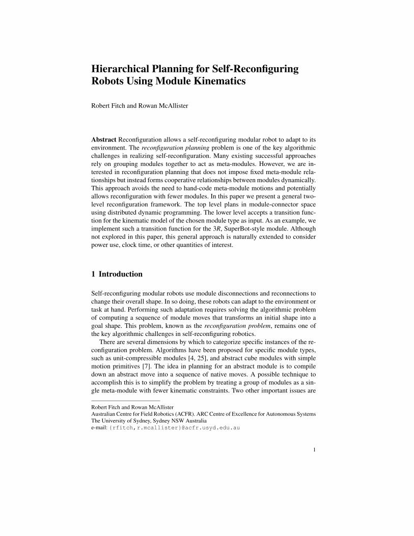
Fig. 2: M−C space is a generalization of the Sliding Cube representation to anymodule type. The Sliding Cube abstraction, (a), has a connection on every face.Other module types, such as SuperBot-style modules, (b), and Roombot-style mod-ules [1], (c), do not. M−C space is simply defined as the set of all module-connectorpairs.


The value function is stored in a distributed fashion. Each module stores the valueof states corresponding to its connectors. The MDP is solved using asynchronousdistributed dynamic programming implemented with message passing. An update isperformed when a module receives a message with a value for a nearby state. Usingthe transition function, the module updates its local value function and sends thesenew values to its neighbors. This process is guaranteed to converge in polynomialtime in the number of states [17]. A moving module queries the value function bysending a request to its connected neighbors. After a move, changed values are againsent to neighbors and the value function is updated.

3.2 MDP Planning with Native Module Kinematics

Building on the Sliding Cube MDP formulation, we now introduce a new MDPformulation that replaces the Sliding Cube and instead assumes the availability ofa kinematic model for a physical module. Instead of abstract motion primitives,motion primitives now correspond to changes in module joint angle and connectorstate. Because actions are no longer unit-time, this is technically a semi-markovdecision problem (SMDP) [2]. However, for the purposes of this paper we assumeunit-time actions. The SMDP formulation allows more sophisticated optimization(time, power, etc.) but we will leave this for future work.

To define the state space, we first define the set of module-connector pairs, or M-C space. Fig. 2 illustrates sample M−C states for three different module types. The

M

C

s0

s1

s2

s3

s0:

s1:

s2:

s3:

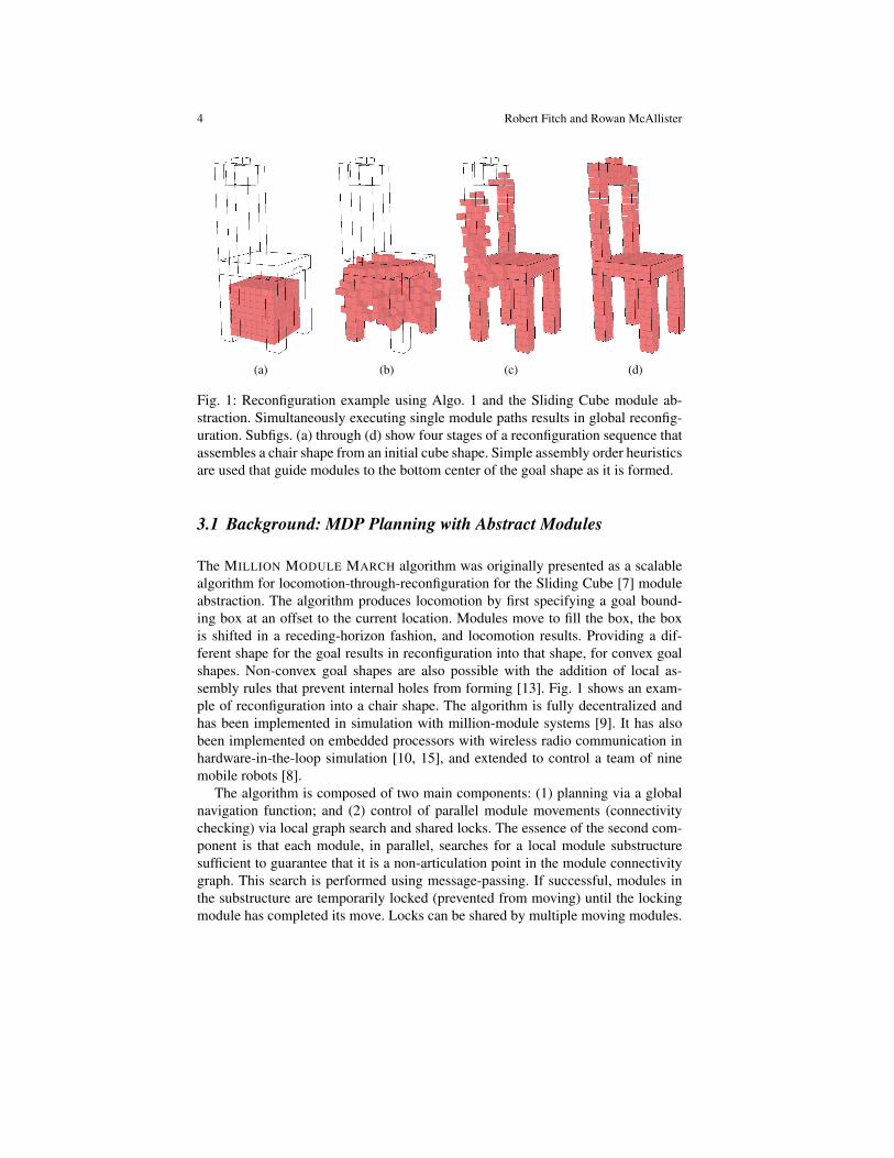
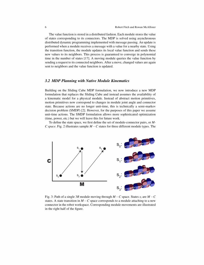
Fig. 3: Path of a single 3R module moving through M−C space. States si are M−Cstates. A state transition in M−C space corresponds to a module attaching to a newconnector in the robot workspace. Corresponding module movements are illustratedin the right half of the figure.


entire set is not necessarily reachable. One obvious example of a non-reachable stateis a connector that is occupied (connected to another module). In general, reacha-bility is determined by the transition function. The transition function, in turn, ispartially determined by the robot configuration topology. Therefore, connectivity ofM−C space changes with reconfiguration. A module with k connectors can poten-tially occupy k M-C states simultaneously. Our state space S is therefore defined asthe set of all k-tuples of M−C states, including a null M−C state that models a freeconnector. Fig. 3 shows an example of a single module making state transitions inM−C space and the corresponding module movements in a sample configuration.

The set of actions is defined by the kinematic model. We assume that an actionconsists of a set of joint angle increments and connection/disconnection actions. Anaction can involve a single module, or a module plus one or more helper modules.

Actions result in changing state. This means that the set of occupied M−C stateswill change following a successful action. An action that fails or otherwise does notresult in a state change is a null action. The transition model defines this change,mapping a state-action pair to a resulting state: T (s,a) = s′, where s ∈ S, s′ ∈ S,and a ∈ A. The transition function must take into account surrounding modules.The potential for collision means that not all actions are available at all times. Thetransition function can be stochastic.

The reward function is -1 for every action. This attempts to minimize the totalnumber of actions. A more sophisticated reward function can be used to minimizeother quantities, such as time, power use, heterogeneous modules, etc. Further, thereward function can be modified during reconfiguration to allow the robot to adaptto changes. However, we do not consider these possibilities in this paper.

3.3 Hierarchical Reconfiguration Algorithm

Having formulated the MDP, we solve using dynamic programming. To allowmodules to move in parallel, we integrate the parallel movement control approachfrom MILLION MODULE MARCH. To prevent collisions, we lock all moduleswithin the workspace of a moving module. The algorithm is listed in pseudocode as

Algorithm 1 General framework for reconfiguration.T : a transition functionG: a goal shapec: the current robot configuration

Generate value function V for c given T and G using dynamic programmingrepeat

Find mobile modulesMove mobile modules one step according to VRecompute V using new configuration c′

until all modules in goal


Algo. 1. Transition function T , goal configuration G, and start configuration c areassumed as input. In parallel, modules follow a path to the goal by chaining togethera sequence of state transitions. Within the goal, modules are guided by local assem-bly order heuristics as above. The algorithm terminates when all modules are in thegoal.

The value function is recomputed as the robot configuration changes, as de-scribed in Sect. 3.1. The MDP will converge in polynomial time [17]. Convergenceof the robot to the goal shape depends on the transition function supplied.

4 A Local Kinematic Planner for 3R Modules

In this section, we flesh out Algo. 1 by defining a transition function based onmodule kinematics. There are many ways to do this in general. We have chosen toview the problem as motion planning for an n−link kinematic chain among regularorthohedral obstacles. Motion planning in high-dimensional spaces is computation-ally intensive. By imposing this strict structure, we can use a simple grid searchmethod for motion planning. We illustrate this technique with the 3R (SuperBot-style) module.

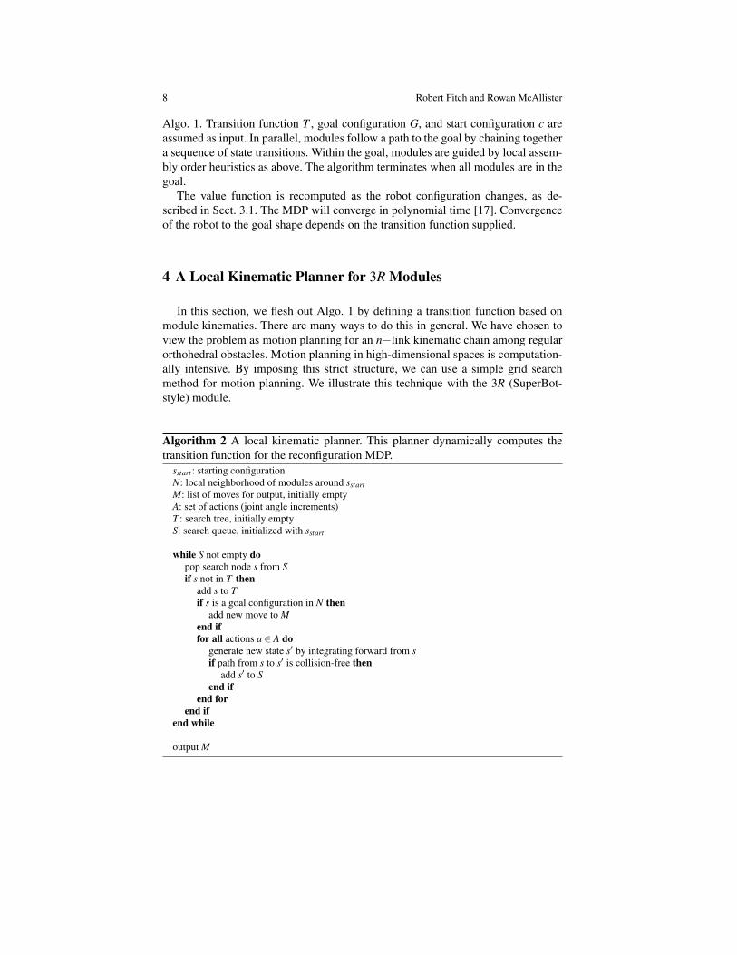
Algorithm 2 A local kinematic planner. This planner dynamically computes thetransition function for the reconfiguration MDP.

sstart : starting configurationN: local neighborhood of modules around sstartM: list of moves for output, initially emptyA: set of actions (joint angle increments)T : search tree, initially emptyS: search queue, initialized with sstart

while S not empty dopop search node s from Sif s not in T then

add s to Tif s is a goal configuration in N then

add new move to Mend iffor all actions a ∈ A do

generate new state s′ by integrating forward from sif path from s to s′ is collision-free then

add s′ to Send if

end forend if

end while

output M


(a) (b) (c) (d)

(e) (f) (g) (h)

(i) (j) (k) (l)

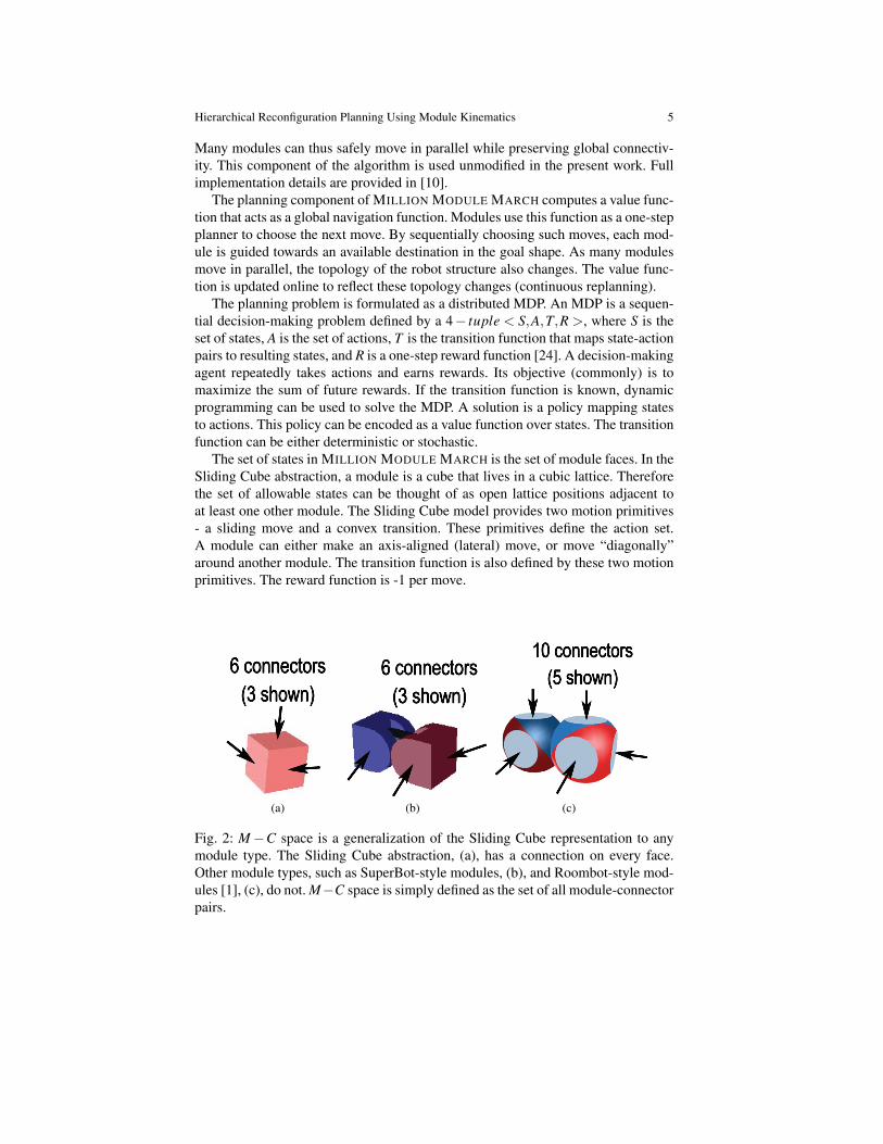
Fig. 4: Workspace reachability. Subfigs. (a) through (d) show sample configurationsreachable with a helper module attached in an end-to-end configuration. Likewise,Subfigs. (e) through (h) show samples reachable from an end-to-side configuration.Subfigs. (i) through (l) correspond to a side-to-side configuration.

M−C−O−Θ space is M−C space augmented by adding two extra dimensions,O ∈ {e,s} and Θ ∈ {0,90,180,270}, that represent how a module is connected tothe M−C pair. Due to connector symmetry, we can encode which connector isconnected by specifying and end (e) or a side (s). The Θ dimension encodes rotationrepresented discretely in 90-degree increments.

We consider two cases for planning. The first is single module motion. Given astarting (m,c,o,θ) state, lattice (workspace) position, and vector of joint angles x,we use the forward kinematics of the 3R module to determine the position of itsconnectors in the workspace. We then consider the set of actions formed by all per-mutations of discrete 90-degree increments/decrements of joint angles. We iteratethrough this set of actions. At each iteration, we add the joint angle increments tothe initial position, resulting in a new joint angle vector x′. We again use the for-ward kinematics to compute the new position of connectors in workspace. If noconnectors are in a position to connect to some other connector in the neighbor-hood, this configuration is discarded. Otherwise we perform collision checking in


(a) (b) (c)

(d) (e) (f)

(g) (h) (i)

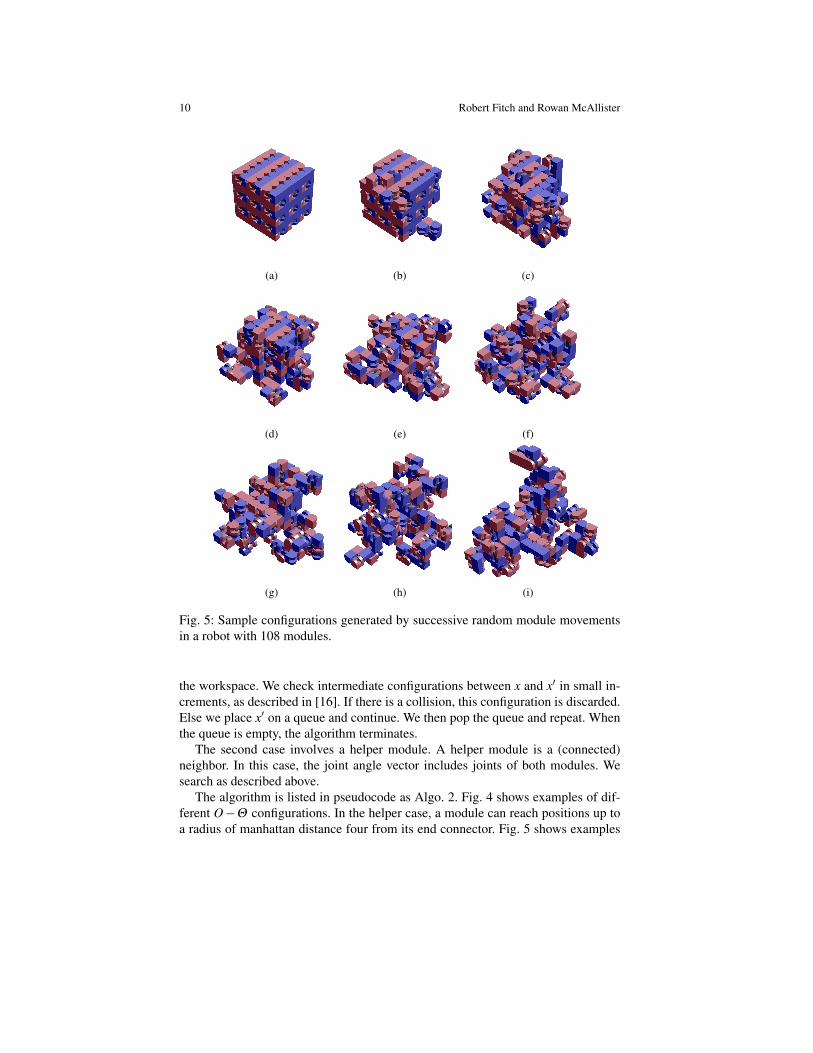
Fig. 5: Sample configurations generated by successive random module movementsin a robot with 108 modules.

the workspace. We check intermediate configurations between x and x′ in small in-crements, as described in [16]. If there is a collision, this configuration is discarded.Else we place x′ on a queue and continue. We then pop the queue and repeat. Whenthe queue is empty, the algorithm terminates.

The second case involves a helper module. A helper module is a (connected)neighbor. In this case, the joint angle vector includes joints of both modules. Wesearch as described above.

The algorithm is listed in pseudocode as Algo. 2. Fig. 4 shows examples of dif-ferent O−Θ configurations. In the helper case, a module can reach positions up toa radius of manhattan distance four from its end connector. Fig. 5 shows examples


drawn from a sequence of configurations generated by successive random modulemovements.

Because we search all joint angle positions, the running time of this algorithmis exponential in the number of joint angles. For constant-length chains of helpermodules, time is constant (albeit with a potentially large constant factor). For two 3Rmodules, the size of the search space is 3∗4∗3∗3∗4∗3 = 1296. This is reasonableto implement with modest embedded computational resources, even consideringthat in computing the value function, each module must perform this computationfor each possible (o,θ) pair (2∗4 = 8) and each of its open connectors.

(a) (b) (c)

(d) (e) (f)

(g) (h) (i)

Fig. 6: Nine modules reconfiguring from a line shape into a box shape.


(a) (b) (c)

(d) (e) (f)

(g) (h) (i)

Fig. 7: Eight modules reconfiguring from an initial cuboid configuration into a goalconfiguration specified by the wire-frame bounding box shown.

4.1 Implementation

We implemented the reconfiguration algorithm in the SRSim simulation environ-ment [7], with SuperBot graphics rendered by a simulation developed at ISI. Col-lision checking is implemented by testing for intersections between the boundingbox surrounding each module part and those surrounding modules in its neighbor-hood. Configuration space is represented as a 6D grid corresponding to module jointangles. The grid can represent one helper module in addition to the main module.Fig. 6 shows an example of nine modules reconfiguring from a line shape into a box.Fig. 7 shows an example reconfiguration between two cuboid configurations.


5 Discussion and Future Work

We have presented a general framework for reconfiguration and an example im-plementation for SuperBot-style modules. Because this simple implementation isexponential in the degrees of freedom of the kinematic chain, this planner is suitedmainly to lattice-based and hybrid robot types. A planner for chain-based robots(with short chains) could possibly be developed. We have not yet explored the po-tential in optimizing for quantities other than number of connection/disconnectioncycles, but this should be a promising avenue. So far we have been concerned onlywith finding a feasible reconfiguration plan, but another interesting problem wouldbe to attempt to prove an approximation to optimal reconfiguration. One idea is tobuild on the lower-bound construction for reconfiguration [18] and attempt to provean upper-bound on the maximum deviation from shortest path taken by any modulein travelling to the goal.

We are currently implementing our algorithm in a decentralized fashion inhardware-in-the-loop simulation [15]. Computation and communication run on em-bedded processors but actuation is simulated on a desktop computer. It is also ourintention to test the algorithm on real robots. One possible platform is a new mod-ule we are currently constructing. This module has SuperBot-style kinematics com-bined with a novel connection mechanism based on grippers or pincers. We wouldalso like to implement and test our algorithm on other module types.

Acknowledgements This work is supported by the ARC Centre of Excellence programme,funded by the Australian Research Council (ARC) and the New South Wales (NSW) State Gov-ernment. Many thanks to Surya Singh for lending expertise in robot kinematics. The SuperBotsimulator was written by David Brandt under the auspices of ISI.

References

1. Asadpour, M., Sproewitz, A., Billard, A., Dillenbourg, P., Ijspeert, A.J.: Graph signature forself-reconfiguration planning. In: Proc. of the IEEE/RSJ IROS, pp. 863–869 (2008)

2. Barto, A., Mahadevan, S.: Recent advances in hiearchical reinforcement learning. SpecialIssue on Reinforcement Learning, Discrete Event Systems Journal 13, 41–77 (2003)

3. Butler, Z., Kotay, K., Rus, D., Tomita, K.: Generic decentralized locomotion control for lattice-based self-reconfigurable robots. Int. J. Rob. Res. 23(9) (2004)

4. Butler, Z., Rus, D.: Distributed motion planning for modular robots with unit-compressiblemodules. Int. J. Rob. Res. 22(9), 699–716 (2003)

5. Chiang, C.H., Chirikjian, G.: Modular robot motion planning using similarity metrics. Au-tonomous Robots 10(1), 91–106 (2001)

6. Christensen, D., Stoy, K.: Selecting a meta-module to shape-change the atron self-reconfigurable robot. In: Proc. of IEEE ICRA, pp. 2532 –2538 (2006)

7. Fitch, R.: Heterogeneous self-reconfiguring robotics. Ph.D. thesis, Dartmouth College (2004)8. Fitch, R., Alempijevic, A., Lal, R.: A self-reconfiguring team of mobile robots. In: Proc. of

IEEE ICRA, Workshop on Network Science and Systems in Multi-Robot Autonomy (2010)9. Fitch, R., Butler, Z.: Million module march: Scalable locomotion for large self-reconfiguring

robots. Int. J. Rob. Res. 27(3-4), 331–343 (2008)10. Fitch, R., Lal, R.: Experiments with a ZigBee wireless communication system for self-

reconfiguring modular robots. In: Proc. of IEEE ICRA, pp. 1947–1952 (2009)


11. Hou, F., Shen, W.M.: Distributed, dynamic, and autonomous reconfiguration planning forchain-type self-reconfigurable robots. In: Proc. of IEEE ICRA (2008)

12. Hou, F., Shen, W.M.: On the complexity of optimal reconfiguration planning for modularreconfigurable robots. In: Proc. of IEEE ICRA (2010)

13. Itzstein, B.: Assembly order planning for stable self-reconfiguration of modular robots. Un-dergraduate thesis, The University of Sydney (2009)

14. Kotay, K., Rus, D.: Algorithms for self-reconfiguring molecule motion planning. In: Proc. ofthe IEEE/RSJ IROS (2000)

15. Lal, R., Fitch, R.: A hardware-in-the-loop simulator for distributed robotics. In: Proc. ofARAA Australasian Conference on Robotics and Automation (ACRA) (2009)

16. LaValle, S.M.: Planning Algorithms. Cambridge University Press, Cambridge, U.K. (2006)17. Littman, M.L., Dean, T.L., Kaelbling, L.P.: On the complexity of solving markov decision

problems. In: Proc. of UAI, pp. 394–402 (1995)18. Pamecha, A., Ebert-Uphoff, I., Chirikjian, G.: Useful metrics for modular robot motion plan-

ning. IEEE Trans. on Robotics and Automation 13(4), 531–45 (1997)19. Prevas, K.C., Unsal, C., Efe, M.O., Khosla, P.K.: A hierarchical motion planning strategy for

a uniform self-reconfigurable modular robotic system. In: Proc. of IEEE ICRA (2002)20. R.Fitch, Rus, D.: Self-reconfiguring robots in the USA. Journal of the Robotics Society of

Japan 21(8), 4–10 (2003)21. Salemi, B., Moll, M., Shen, W.M.: SUPERBOT: A deployable, multi-functional, and modular

self-reconfigurable robotic system. In: Proc. of IEEE/RSJ IROS (2006)22. Stoy, K.: Controlling self-reconfiguration using cellular automata and gradients. In: Proceed-

ings of IAS-8 (2004)23. Stoy, K., Nagpal, R.: Self-reconfiguration using directed growth. In: 7th International Sympo-

sium on Distributed Autonomous Robotic Systems (DARS’04) (2004)24. Sutton, R., Barto, A.: Reinforcement Learning: An Introduction. MIT Press, Cambridge, MA

(1998)25. Vassilvitskii, S., Yim, M., Suh, J.: A complete, local and parallel reconfiguration algorithm for

cube style modular robots. In: Proc. of IEEE ICRA, pp. 117–22 (2002)26. Yim, M., Shen, W.M., Salemi, B., Rus, D., Moll, M., Lipson, H., Klavins, E., Chirikjian, G.:

Modular self-reconfigurable robot systems. IEEE Robot. Automat. Mag. 14(1), 43–52 (2007)27. Yoshida, E., Matura, S., Kamimura, A., Tomita, K., Kurokawa, H., Kokaji, S.: A Self-

Reconfigurable Modular Robot: Reconfiguration Planning and Experiments. Int. J. Rob. Res.pp. 903–915 (2002)

Documents

Hierarchical Planning for Self-Reconﬁguring Robots Using