SANDIA REPORTSAND2014-18565Unlimited ReleasePrinted October 2014

Hierarchical Multiscale MethodDevelopment for Peridynamics

Stewart A. SillingJames V. Cox

Prepared bySandia National LaboratoriesAlbuquerque, New Mexico 87185 and Livermore, California 94550

Sandia National Laboratories is a multi-program laboratory managed and operated by Sandia Corporation,a wholly owned subsidiary of Lockheed Martin Corporation, for the U.S. Department of Energy’sNational Nuclear Security Administration under contract DE-AC04-94AL85000.

Approved for public release; further dissemination unlimited.

Issued by Sandia National Laboratories, operated for the United States Department of Energyby Sandia Corporation.

NOTICE: This report was prepared as an account of work sponsored by an agency of the UnitedStates Government. Neither the United States Government, nor any agency thereof, nor anyof their employees, nor any of their contractors, subcontractors, or their employees, make anywarranty, express or implied, or assume any legal liability or responsibility for the accuracy,completeness, or usefulness of any information, apparatus, product, or process disclosed, or rep-resent that its use would not infringe privately owned rights. Reference herein to any specificcommercial product, process, or service by trade name, trademark, manufacturer, or otherwise,does not necessarily constitute or imply its endorsement, recommendation, or favoring by theUnited States Government, any agency thereof, or any of their contractors or subcontractors.The views and opinions expressed herein do not necessarily state or reflect those of the UnitedStates Government, any agency thereof, or any of their contractors.

Printed in the United States of America. This report has been reproduced directly from the bestavailable copy.

Available to DOE and DOE contractors fromU.S. Department of EnergyOffice of Scientific and Technical InformationP.O. Box 62Oak Ridge, TN 37831

Telephone: (865) 576-8401Facsimile: (865) 576-5728E-Mail: reports@adonis.osti.govOnline ordering: http://www.osti.gov/bridge

Available to the public fromU.S. Department of CommerceNational Technical Information Service5285 Port Royal RdSpringfield, VA 22161

Telephone: (800) 553-6847Facsimile: (703) 605-6900E-Mail: orders@ntis.fedworld.govOnline ordering: http://www.ntis.gov/help/ordermethods.asp?loc=7-4-0#online

DE

PA

RT

MENT OF EN

ER

GY

• • UN

IT

ED

STATES OFA

M

ER

IC

A

2

SAND2014-18565Unlimited Release

Printed October 2014

Hierarchical Multiscale Method Developmentfor Peridynamics

Stewart A. SillingMultiscale Science DepartmentSandia National Laboratories

P.O Box 5800Albuquerque, NM 87185-1322

James V. CoxSolid Mechanics DepartmentSandia National Laboratories

P.O. Box 5800Albuquerque, NM 87185-0840

Abstract

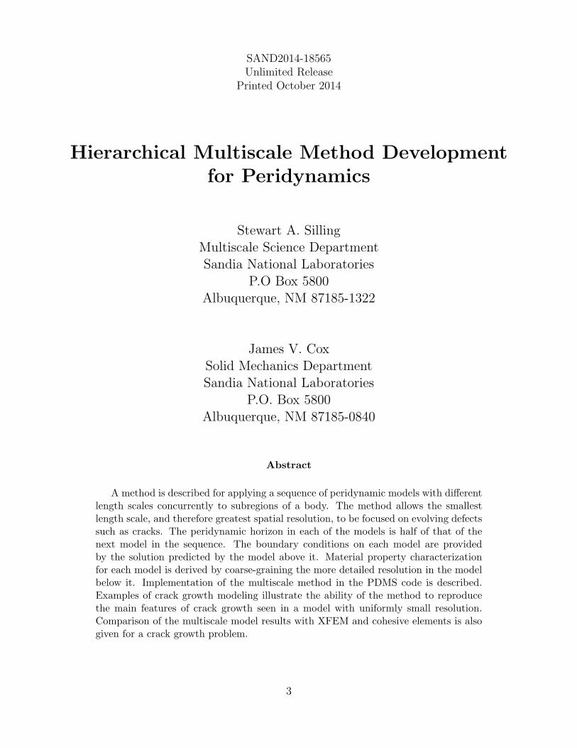
A method is described for applying a sequence of peridynamic models with differentlength scales concurrently to subregions of a body. The method allows the smallestlength scale, and therefore greatest spatial resolution, to be focused on evolving defectssuch as cracks. The peridynamic horizon in each of the models is half of that of thenext model in the sequence. The boundary conditions on each model are providedby the solution predicted by the model above it. Material property characterizationfor each model is derived by coarse-graining the more detailed resolution in the modelbelow it. Implementation of the multiscale method in the PDMS code is described.Examples of crack growth modeling illustrate the ability of the method to reproducethe main features of crack growth seen in a model with uniformly small resolution.Comparison of the multiscale model results with XFEM and cohesive elements is alsogiven for a crack growth problem.

3

Acknowledgments

This work was sponsored by the Joint DOD/DoE Munitions Technology Program at SandiaNational Laboratories.

4

Contents

1 Introduction . . . . . . . . . . . . . . . . . . . . . . . . . . . . . . . . . . . . . . . . . . . . . . . . . . . . . . . . . . . . . . . . . . . . . 72 Multiscale method . . . . . . . . . . . . . . . . . . . . . . . . . . . . . . . . . . . . . . . . . . . . . . . . . . . . . . . . . . . . . . . 113 Numerical implementation. . . . . . . . . . . . . . . . . . . . . . . . . . . . . . . . . . . . . . . . . . . . . . . . . . . . . . . . 154 Node creation and deletion . . . . . . . . . . . . . . . . . . . . . . . . . . . . . . . . . . . . . . . . . . . . . . . . . . . . . . . 175 Example . . . . . . . . . . . . . . . . . . . . . . . . . . . . . . . . . . . . . . . . . . . . . . . . . . . . . . . . . . . . . . . . . . . . . . . . . 186 Discussion. . . . . . . . . . . . . . . . . . . . . . . . . . . . . . . . . . . . . . . . . . . . . . . . . . . . . . . . . . . . . . . . . . . . . . . . 27

Figures

1 Family of a material point x. . . . . . . . . . . . . . . . . . . . . . . . . . . . . . . . . . . . . . . . . 82 Boundary conditions (volume constraints) are applied to a peridynamic body

B in a subregion of finite volume R. . . . . . . . . . . . . . . . . . . . . . . . . . . . . . . . . . . 103 Levels surrounding a crack tip process zone. . . . . . . . . . . . . . . . . . . . . . . . . . . . 124 Higher levels have larger horizons. . . . . . . . . . . . . . . . . . . . . . . . . . . . . . . . . . . . 135 Schematic of interactions between levels. . . . . . . . . . . . . . . . . . . . . . . . . . . . . . . 136 Compact tension specimen with a 5 mm pre-existing edge crack. This schematic

of the model does not include extensions of the domain on the bottom to applydisplacement boundary conditions to the PDMS model. . . . . . . . . . . . . . . . . . . 20

7 Simulated growth of an edge crack. Left: colors indicate bond strain. Right:crack process zone and surrounding higher-level subregions. . . . . . . . . . . . . . . . 21

8 Comparison of predictions for the edge crack growth problem using differentnumbers multiscale levels. . . . . . . . . . . . . . . . . . . . . . . . . . . . . . . . . . . . . . . . . . . 22

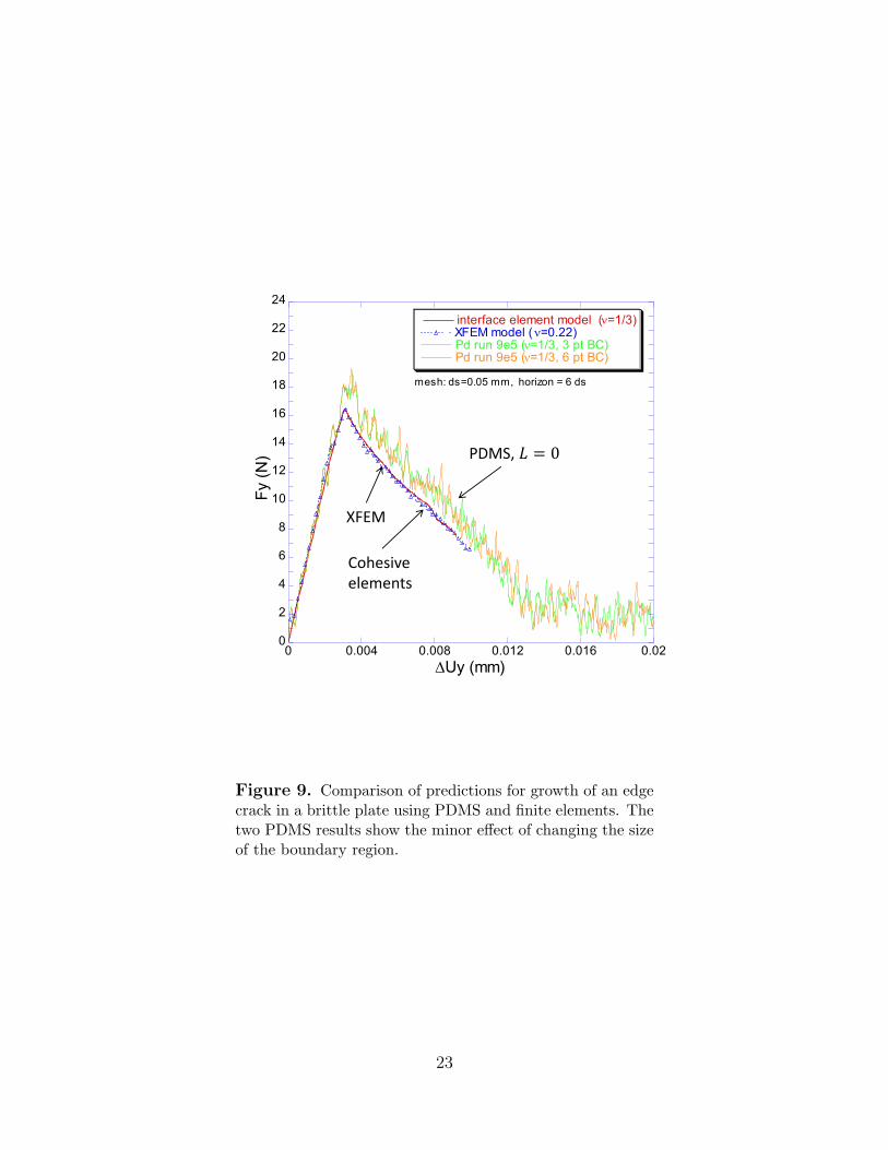
9 Comparison of predictions for growth of an edge crack in a brittle plate usingPDMS and finite elements. The two PDMS results show the minor effect ofchanging the size of the boundary region. . . . . . . . . . . . . . . . . . . . . . . . . . . . . . . 23

10 Comparison of predictions for growth of an edge crack in a brittle plate usingPDMS and finite elements. The three PDMS results show the minor effect ofchanging the size of the grid and the grid-scaled horizon. . . . . . . . . . . . . . . . . . 24

11 High-rate loading of a plate with an edge crack results in crack branching. . . . 2512 Crack branching in a heterogeneous medium with hard inclusions. . . . . . . . . . 26

5

6

1 Introduction

The peridynamic theory of solid mechanics [1, 2] is designed to unify the mathematical andcomputational modeling of continuous media, crack growth, and discrete particles. It accom-plishes this by using integro-differential equations, rather than partial differential equations,as the basic mathematical tools. The integro-differential equations do not require the evalu-ation of spatial derivatives of the deformation or of a stress field. Hence, they are applicableeven when the deformation contains discontinuities such as cracks. Using generalized func-tions, the same peridynamic equations also apply to systems of discrete particles, includingmolecular dynamics.

In the peridynamic theory, the equation of motion is given by

ρ(x)u(x, t) =

∫Hx

f(q,x, t) dVq + b(x, t) (1)

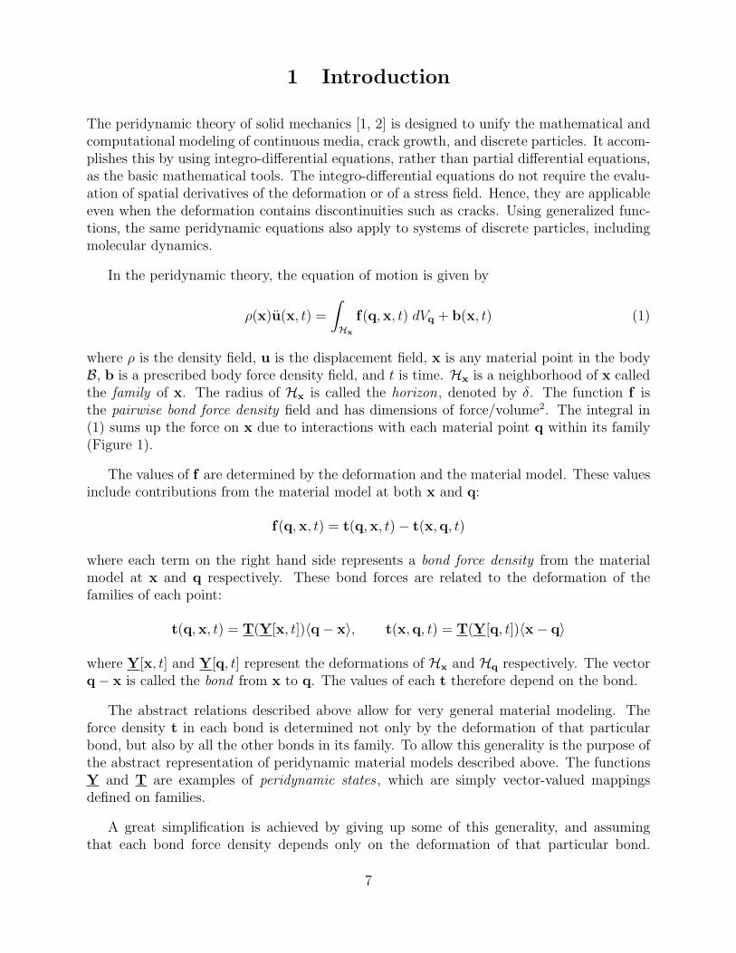
where ρ is the density field, u is the displacement field, x is any material point in the bodyB, b is a prescribed body force density field, and t is time. Hx is a neighborhood of x calledthe family of x. The radius of Hx is called the horizon, denoted by δ. The function f isthe pairwise bond force density field and has dimensions of force/volume2. The integral in(1) sums up the force on x due to interactions with each material point q within its family(Figure 1).

The values of f are determined by the deformation and the material model. These valuesinclude contributions from the material model at both x and q:

f(q,x, t) = t(q,x, t)− t(x,q, t)

where each term on the right hand side represents a bond force density from the materialmodel at x and q respectively. These bond forces are related to the deformation of thefamilies of each point:

t(q,x, t) = T(Y[x, t])〈q− x〉, t(x,q, t) = T(Y[q, t])〈x− q〉

where Y[x, t] and Y[q, t] represent the deformations of Hx and Hq respectively. The vectorq− x is called the bond from x to q. The values of each t therefore depend on the bond.

The abstract relations described above allow for very general material modeling. Theforce density t in each bond is determined not only by the deformation of that particularbond, but also by all the other bonds in its family. To allow this generality is the purpose ofthe abstract representation of peridynamic material models described above. The functionsY and T are examples of peridynamic states , which are simply vector-valued mappingsdefined on families.

A great simplification is achieved by giving up some of this generality, and assumingthat each bond force density depends only on the deformation of that particular bond.

7

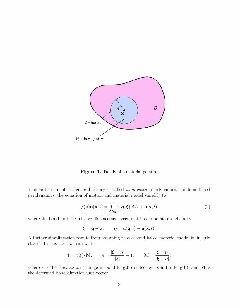
Figure 1. Family of a material point x.

This restriction of the general theory is called bond-based peridynamics. In bond-basedperidynamics, the equation of motion and material model simplify to

ρ(x)u(x, t) =

∫Hx

f(η, ξ) dVξ + b(x, t) (2)

where the bond and the relative displacement vector at its endpoints are given by

ξ = q− x, η = u(q, t)− u(x, t).

A further simplification results from assuming that a bond-based material model is linearlyelastic. In this case, we can write

f = c(ξ)sM, s =|ξ + η||ξ|

− 1, M =ξ + η

|ξ + η|,

where s is the bond strain (change in bond length divided by its initial length), and M isthe deformed bond direction unit vector.

8

Damage can be incorporated into a bond-based peridynamic model using the idea ofbond breakage. When a bond’s deformation reaches some critical condition, the bond breaksirreversibly, meaning that it no longer carries any load. One way of expressing this is througha history-dependent bond damage variable µ that changes irreversibly from 1 to 0 at thetime of bond breakage:

c(ξ, t) = c0(ξ)µ(ξ, t), (3)

where c0 is the undamaged spring constant. In the special case of constant c0 independentof ξ (that is, constant within the family), the calibration of the model for three-dimensionalformulations [3] leads to

c0 =18k

πδ4. (4)

The resulting bond-based material model is called the prototype elastic brittle (PMB) model.Although many bond damage laws are possible, the most widely used is based on criticalbond strain:

s(ξ, t∗) > s∗ =⇒ µ(ξ, t) = 0 for all t ≥ t∗ (5)

where s∗ is a prescribed critical bond breakage strain and t∗ is the time of bond breakage(usually not known in advance of modeling an application).

The horizon δ represents the maximum interaction distance for material points. Pointsx and q that are separated by an initial distance greater than δ do not interact, and aretherefore excluded from the volume of integration Hx in the equation of motion. When thescale of the modeling resolves the materials structure, the horizon is treated like a materialproperty – a length scale correlated with the underlying material structure. When the scale ofthe modeling represents the material as a homogenous continuum, the horizon is a numericalparameter that is frequently chosen as a matter of convenience, since a peridynamic materialmodel can usually be fitted to measurable material properties for any given value of δ.

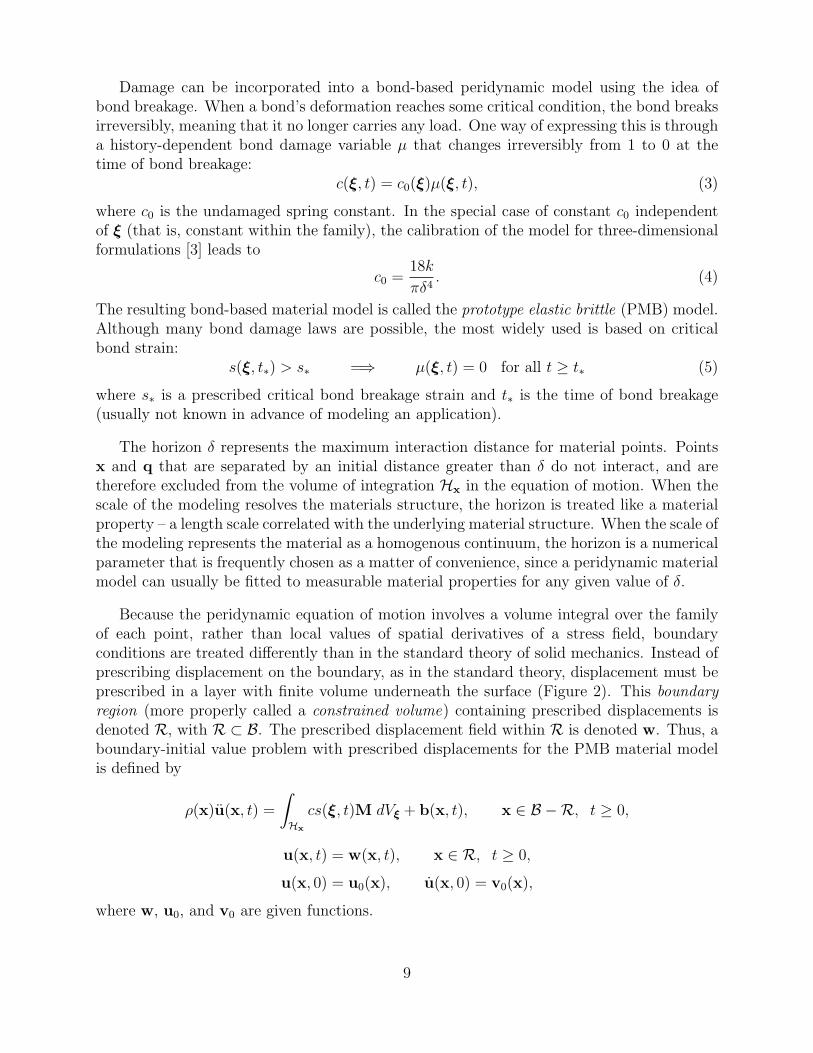
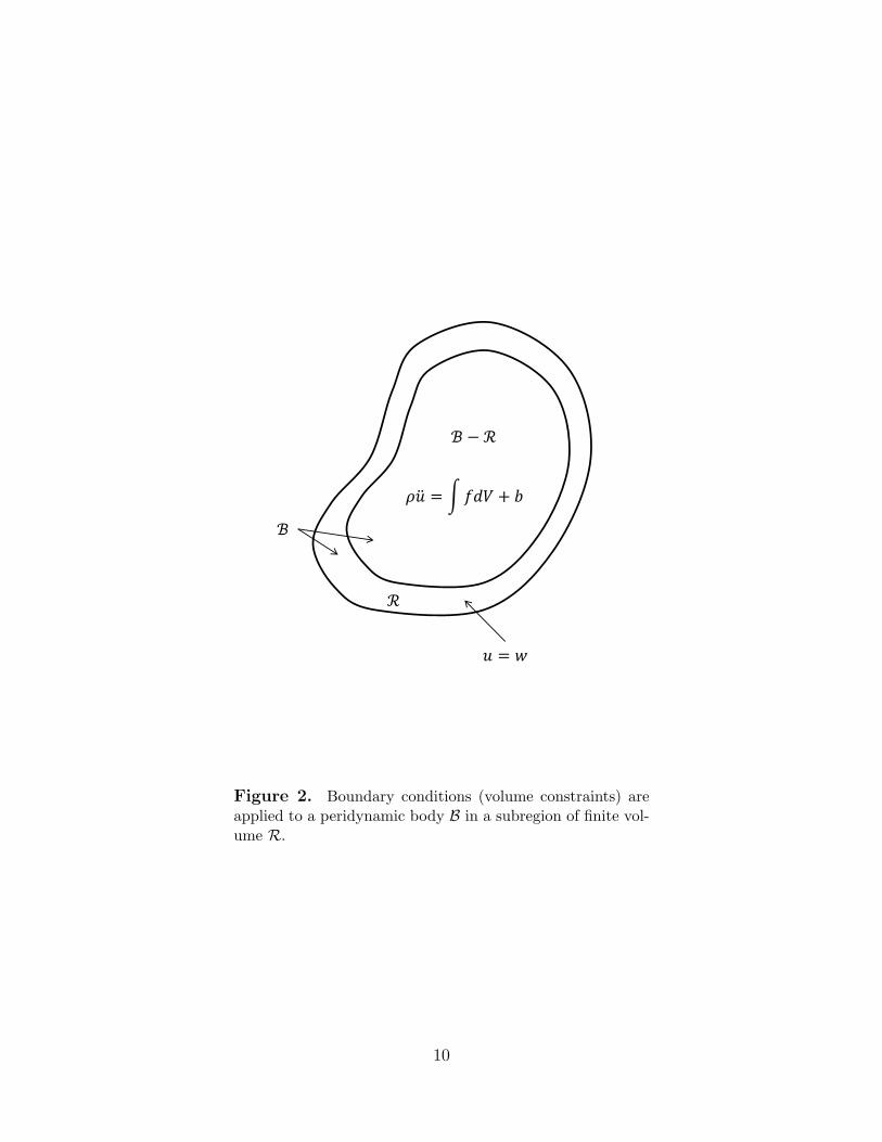
Because the peridynamic equation of motion involves a volume integral over the familyof each point, rather than local values of spatial derivatives of a stress field, boundaryconditions are treated differently than in the standard theory of solid mechanics. Instead ofprescribing displacement on the boundary, as in the standard theory, displacement must beprescribed in a layer with finite volume underneath the surface (Figure 2). This boundaryregion (more properly called a constrained volume) containing prescribed displacements isdenoted R, with R ⊂ B. The prescribed displacement field within R is denoted w. Thus, aboundary-initial value problem with prescribed displacements for the PMB material modelis defined by

ρ(x)u(x, t) =

∫Hx

cs(ξ, t)M dVξ + b(x, t), x ∈ B −R, t ≥ 0,

u(x, t) = w(x, t), x ∈ R, t ≥ 0,

u(x, 0) = u0(x), u(x, 0) = v0(x),

where w, u0, and v0 are given functions.

9

ℬ

ℛ

𝑢 = 𝑤

ℬ − ℛ

𝜌𝑢 = 𝑓𝑑𝑉 + 𝑏

Figure 2. Boundary conditions (volume constraints) areapplied to a peridynamic body B in a subregion of finite vol-ume R.

10

2 Multiscale method

Any application of peridynamics involves a choice of the horizon δ. Unlike more typicalnonlocal models, the length parameter (the horizon in the case of peridynamics) influencesthe region of integration Hx in the equation of motion and the material model. This raisesthe possibility that by varying δ, a multiscale method could be obtained. It is this possibilitythat motivates the method development described in the remainder of this report.

It would be convenient if δ could be prescribed arbitrarily as a function of position andtime within a mathematical model of a body, allowing the smallest length scale to be appliedin the vicinity of small features of interest such as crack tips or other defects. Unfortunately,non-constant values of δ(x, t) result in undesirable artifacts in the predicted displacementfield except in a few special cases.

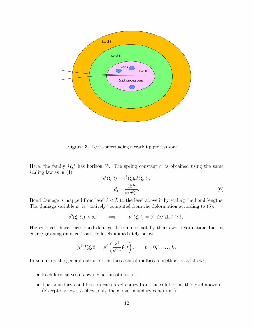
Therefore, we pursue a different strategy for multiscale peridynamics. In this approach, asequence of L+ 1 distinct models called levels is applied to different subregions of the body.Each level, which occupies the subregion B`, has a distinct but constant value of horizondenoted δ`, ` = 0, 1, . . . , L. The level 0 model provides the most detailed resolution and isassumed to contain the “best physics” at the smallest applicable length scale. Successivelevels become progressively more smeared and continuum-like by applying larger lengthscales, and it is assumed that

δ0 < δ1 < · · · < δL.

Each level is a subset of the level above it:

B0 ⊂ B1 ⊂ · · · ⊂ BL.

(Figure 3.) The highest level is identical to the full body:

BL = B.

Let u` denote the displacement field in level `. All the levels obey the global initial conditions.Global body force densities are also applied identically in all levels.

Displacement boundary conditions on each level ` < L are derived from the level aboveit:

u` = u`+1 on R` ⊂ B`+1.

In other words, the boundary displacements in level ` are identical to whatever displacementsare computed in the level above it. In summary, the levels obey a coupled set of initialboundary value problems:

ρ(x)u`(x, t) =

∫Hx

`

c`s`(ξ, t)M dVξ + b(x, t), x ∈ B` −R`, t ≥ 0,

u`(x, t) = u`+1(x, t), x ∈ R`, t ≥ 0,

u`(x, 0) = u0(x), u`(x, 0) = v0(x).

11

Crack process zone

Level 2

Level 1

Level 0 Voids

Figure 3. Levels surrounding a crack tip process zone.

Here, the family Hx` has horizon δ`. The spring constant c` is obtained using the same

scaling law as in (4):c`(ξ, t) = c`0(ξ)µ`(ξ, t),

c`0 =18k

π(δ`)4. (6)

Bond damage is mapped from level ` < L to the level above it by scaling the bond lengths.The damage variable µ0 is “actively” computed from the deformation according to (5):

s0(ξ, t∗) > s∗ =⇒ µ0(ξ, t) = 0 for all t ≥ t∗.

Higher levels have their bond damage determined not by their own deformation, but bycoarse graining damage from the levels immediately below:

µ`+1(ξ, t) = µ`

(δ`

δ`+1ξ, t

), ` = 0, 1, . . . , L.

In summary, the general outline of the hierarchical multiscale method is as follows:

• Each level solves its own equation of motion.

• The boundary condition on each level comes from the solution at the level above it.(Exception: level L obeys only the global boundary condition.)

12

𝛿0 𝛿1 𝛿2

Figure 4. Higher levels have larger horizons.

Level

x

y

Crack 2

1

0

Figure 5. Schematic of interactions between levels.

13

• The damage at each level is coarse-grained up from the level below it. (Exception:damage in level 0 is determined by the deformation and material damage law.)

14

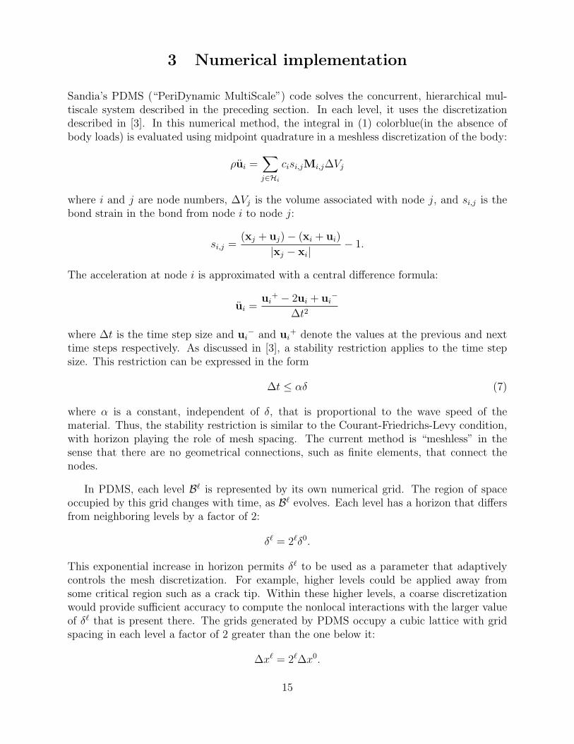
3 Numerical implementation

Sandia’s PDMS (“PeriDynamic MultiScale”) code solves the concurrent, hierarchical mul-tiscale system described in the preceding section. In each level, it uses the discretizationdescribed in [3]. In this numerical method, the integral in (1) colorblue(in the absence ofbody loads) is evaluated using midpoint quadrature in a meshless discretization of the body:

ρui =∑j∈Hi

cisi,jMi,j∆Vj

where i and j are node numbers, ∆Vj is the volume associated with node j, and si,j is thebond strain in the bond from node i to node j:

si,j =(xj + uj)− (xi + ui)

|xj − xi|− 1.

The acceleration at node i is approximated with a central difference formula:

ui =ui

+ − 2ui + ui−

∆t2

where ∆t is the time step size and ui− and ui

+ denote the values at the previous and nexttime steps respectively. As discussed in [3], a stability restriction applies to the time stepsize. This restriction can be expressed in the form

∆t ≤ αδ (7)

where α is a constant, independent of δ, that is proportional to the wave speed of thematerial. Thus, the stability restriction is similar to the Courant-Friedrichs-Levy condition,with horizon playing the role of mesh spacing. The current method is “meshless” in thesense that there are no geometrical connections, such as finite elements, that connect thenodes.

In PDMS, each level B` is represented by its own numerical grid. The region of spaceoccupied by this grid changes with time, as B` evolves. Each level has a horizon that differsfrom neighboring levels by a factor of 2:

δ` = 2`δ0.

This exponential increase in horizon permits δ` to be used as a parameter that adaptivelycontrols the mesh discretization. For example, higher levels could be applied away fromsome critical region such as a crack tip. Within these higher levels, a coarse discretizationwould provide sufficient accuracy to compute the nonlocal interactions with the larger valueof δ` that is present there. The grids generated by PDMS occupy a cubic lattice with gridspacing in each level a factor of 2 greater than the one below it:

∆x` = 2`∆x0.

15

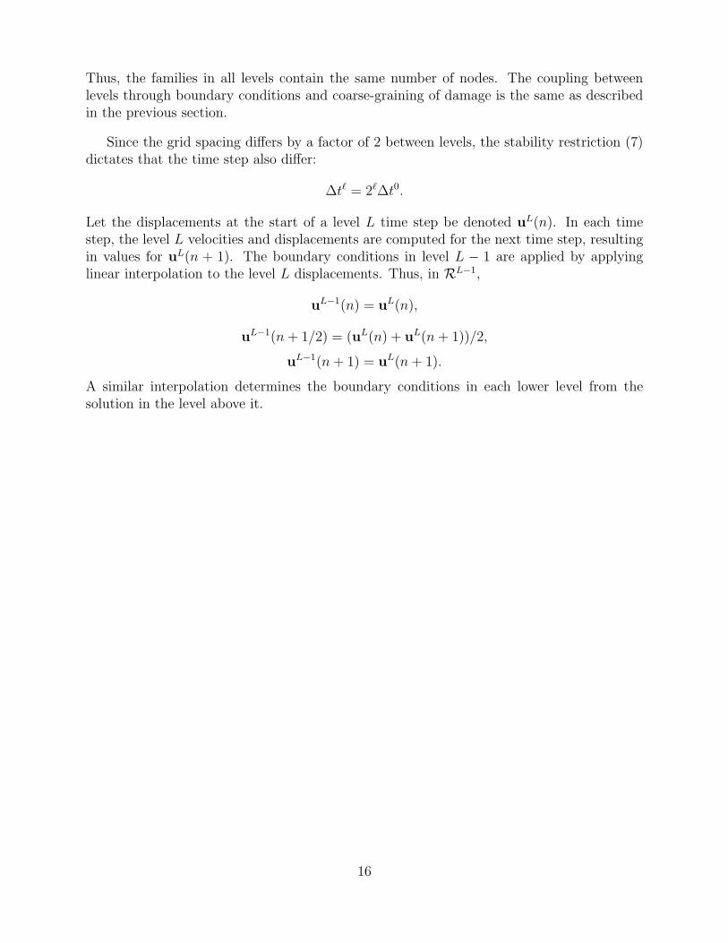
Thus, the families in all levels contain the same number of nodes. The coupling betweenlevels through boundary conditions and coarse-graining of damage is the same as describedin the previous section.

Since the grid spacing differs by a factor of 2 between levels, the stability restriction (7)dictates that the time step also differ:

∆t` = 2`∆t0.

Let the displacements at the start of a level L time step be denoted uL(n). In each timestep, the level L velocities and displacements are computed for the next time step, resultingin values for uL(n + 1). The boundary conditions in level L − 1 are applied by applyinglinear interpolation to the level L displacements. Thus, in RL−1,

uL−1(n) = uL(n),

uL−1(n+ 1/2) = (uL(n) + uL(n+ 1))/2,

uL−1(n+ 1) = uL(n+ 1).

A similar interpolation determines the boundary conditions in each lower level from thesolution in the level above it.

16

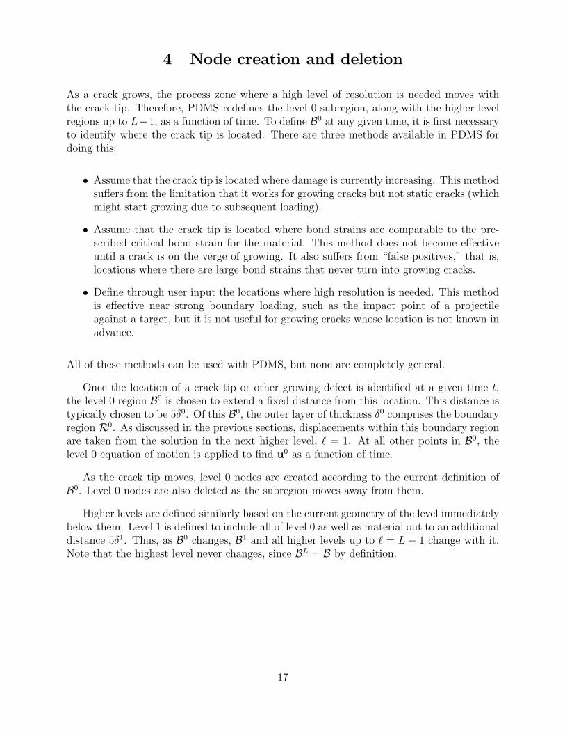
4 Node creation and deletion

As a crack grows, the process zone where a high level of resolution is needed moves withthe crack tip. Therefore, PDMS redefines the level 0 subregion, along with the higher levelregions up to L−1, as a function of time. To define B0 at any given time, it is first necessaryto identify where the crack tip is located. There are three methods available in PDMS fordoing this:

• Assume that the crack tip is located where damage is currently increasing. This methodsuffers from the limitation that it works for growing cracks but not static cracks (whichmight start growing due to subsequent loading).

• Assume that the crack tip is located where bond strains are comparable to the pre-scribed critical bond strain for the material. This method does not become effectiveuntil a crack is on the verge of growing. It also suffers from “false positives,” that is,locations where there are large bond strains that never turn into growing cracks.

• Define through user input the locations where high resolution is needed. This methodis effective near strong boundary loading, such as the impact point of a projectileagainst a target, but it is not useful for growing cracks whose location is not known inadvance.

All of these methods can be used with PDMS, but none are completely general.

Once the location of a crack tip or other growing defect is identified at a given time t,the level 0 region B0 is chosen to extend a fixed distance from this location. This distance istypically chosen to be 5δ0. Of this B0, the outer layer of thickness δ0 comprises the boundaryregion R0. As discussed in the previous sections, displacements within this boundary regionare taken from the solution in the next higher level, ` = 1. At all other points in B0, thelevel 0 equation of motion is applied to find u0 as a function of time.

As the crack tip moves, level 0 nodes are created according to the current definition ofB0. Level 0 nodes are also deleted as the subregion moves away from them.

Higher levels are defined similarly based on the current geometry of the level immediatelybelow them. Level 1 is defined to include all of level 0 as well as material out to an additionaldistance 5δ1. Thus, as B0 changes, B1 and all higher levels up to ` = L− 1 change with it.Note that the highest level never changes, since BL = B by definition.

17

5 Example

Consider the plate with a pre-existing edge crack shown in Figure 6. This compact tensiontype specimen was inspired by a recent problem for a ductile fracture modeling challenge[4]. While this specimen might more typically be used to measure the fracture energy ofa material, here we focus on the crack propagation predicted by the method. Simplifieddisplacement boundary conditions, applied to the lower edges, were substituted for the morecomplex pin connections of the actual specimen. Both boundary conditions produce anincreasing crack opening displacement along the specimen’s edge that causes the crack togrow. As with a double cantilever specimen, one would expect the crack path to be unstable.To compare PDMS model results with those of FE methods using cohesive zone and XFEMcrack growth models, we only consider propagation of a straight crack. The FEM analysesconstrain the crack to a straight path, while the PDMS simulations produce a straight crackpath due to the model symmetry and homogeneity of the material parameters.

In the peridynamics formulation, we do not have an equivalency between the bond failuremodel and a corresponding cohesive zone representation. However, under the assumptionmade in linear elastic fracture mechanics (LEFM) of a small process zone, we expect thetwo formulations to approximate each other, because the results should depend upon thefracture energy alone and not upon the specific traction separation behavior. (In contrast,a “quasi-brittle” problem is characterized by a relatively large process zone for which thetraction separation response can have a significant effect upon the specimen’s response.)

In comparing the PDMS model with FE models, it should be noted that the two ap-proaches approximate LEFM in different senses. To obtain results representative of LEFMfor a cohesive crack model, one would typically hold the fracture energy constant while ex-amining the predicted response for analyses with increasing strength (peak traction in thecohesive zone model). The corresponding critical crack opening would decrease with theincrease of strength eventually yielding results where the size of the cohesive zone is suffi-ciently small to closely approximate LEFM. For the peridynamics analyses one could obtainresults approaching those of LEFM by reducing the size of the level 0 horizon. In this exam-ple problem, the “limiting studies” that one could conduct with the different computationalmethods to approach LEFM are not addressed, so we only anticipate that the results willbe qualitatively close but not as close as the two FEM results (both of which use cohesivezone models).

For a brittle fracture model problem, we assume properties representative of a soda-lime-silicate glass. The assumed fracture energy is 6.5 J/m2, and for the FEM models used incomparison [5] we start with a strength of 27 MPa, which is toward the low end of nominalstrengths for the material. In the FEM results the size of the cohesive zone remained closeto 0.5 mm during the crack propagation [5]. This length was about 10 percent of the originalcrack length and thus about 5 percent of the crack length by the time it had grown another5 mm. Figure 7 depicts the simulated growth of the crack with the PDMS formulation,showing both the bond strains and damage process zone.

18

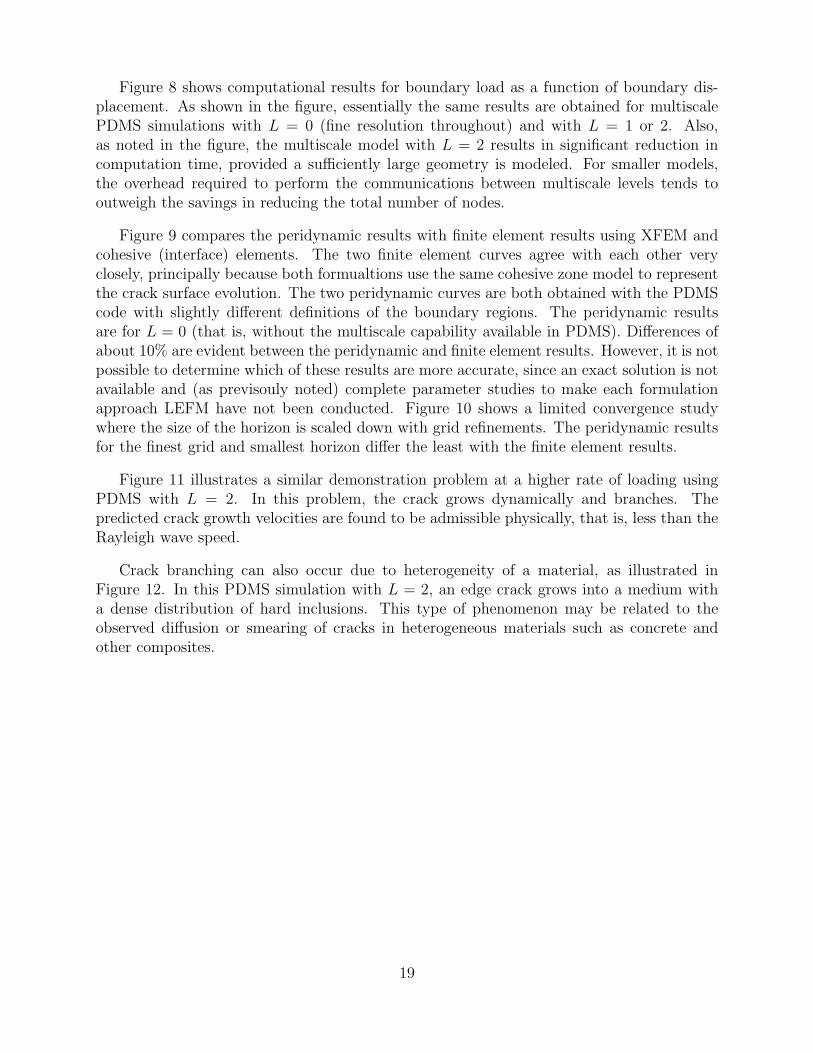
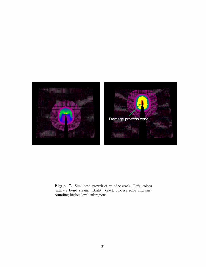
Figure 8 shows computational results for boundary load as a function of boundary dis-placement. As shown in the figure, essentially the same results are obtained for multiscalePDMS simulations with L = 0 (fine resolution throughout) and with L = 1 or 2. Also,as noted in the figure, the multiscale model with L = 2 results in significant reduction incomputation time, provided a sufficiently large geometry is modeled. For smaller models,the overhead required to perform the communications between multiscale levels tends tooutweigh the savings in reducing the total number of nodes.

Figure 9 compares the peridynamic results with finite element results using XFEM andcohesive (interface) elements. The two finite element curves agree with each other veryclosely, principally because both formualtions use the same cohesive zone model to representthe crack surface evolution. The two peridynamic curves are both obtained with the PDMScode with slightly different definitions of the boundary regions. The peridynamic resultsare for L = 0 (that is, without the multiscale capability available in PDMS). Differences ofabout 10% are evident between the peridynamic and finite element results. However, it is notpossible to determine which of these results are more accurate, since an exact solution is notavailable and (as previsouly noted) complete parameter studies to make each formulationapproach LEFM have not been conducted. Figure 10 shows a limited convergence studywhere the size of the horizon is scaled down with grid refinements. The peridynamic resultsfor the finest grid and smallest horizon differ the least with the finite element results.

Figure 11 illustrates a similar demonstration problem at a higher rate of loading usingPDMS with L = 2. In this problem, the crack grows dynamically and branches. Thepredicted crack growth velocities are found to be admissible physically, that is, less than theRayleigh wave speed.

Crack branching can also occur due to heterogeneity of a material, as illustrated inFigure 12. In this PDMS simulation with L = 2, an edge crack grows into a medium witha dense distribution of hard inclusions. This type of phenomenon may be related to theobserved diffusion or smearing of cracks in heterogeneous materials such as concrete andother composites.

19

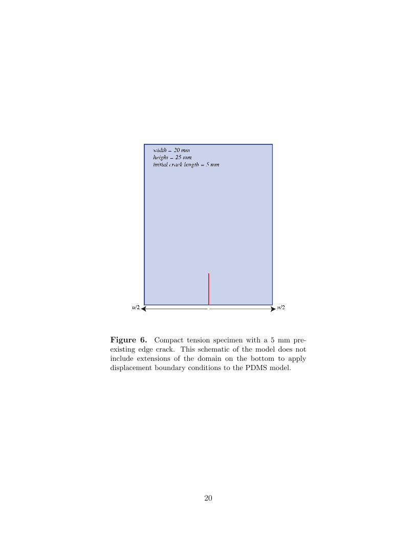
Figure 6. Compact tension specimen with a 5 mm pre-existing edge crack. This schematic of the model does notinclude extensions of the domain on the bottom to applydisplacement boundary conditions to the PDMS model.

20

Damage process zone

Figure 7. Simulated growth of an edge crack. Left: colorsindicate bond strain. Right: crack process zone and sur-rounding higher-level subregions.

21

Level Wall clock time (min) with

28K nodes in coarse grid

Wall clock time (min) with

110K nodes in coarse grid

0 30 168

2 8 16

𝐿 = 0

Bo

un

dar

y lo

ad

Boundary displacement

𝐿 = 1

𝐿 = 2

Figure 8. Comparison of predictions for the edge crackgrowth problem using different numbers multiscale levels.

22

0

2

4

6

8

10

12

14

16

18

20

22

24

0 0.004 0.008 0.012 0.016 0.02

interface element model (=1/3)XFEM model (=0.22)Pd run 9e5 (=1/3, 3 pt BC)Pd run 9e5 (=1/3, 6 pt BC)

Fy (

N)

Uy (mm)

mesh: ds=0.05 mm, horizon = 6 ds

PDMS, 𝐿 = 0

XFEM

Cohesive elements

Figure 9. Comparison of predictions for growth of an edgecrack in a brittle plate using PDMS and finite elements. Thetwo PDMS results show the minor effect of changing the sizeof the boundary region.

23

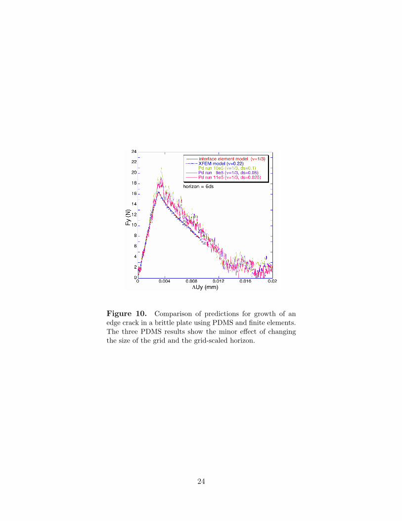
Figure 10. Comparison of predictions for growth of anedge crack in a brittle plate using PDMS and finite elements.The three PDMS results show the minor effect of changingthe size of the grid and the grid-scaled horizon.

24

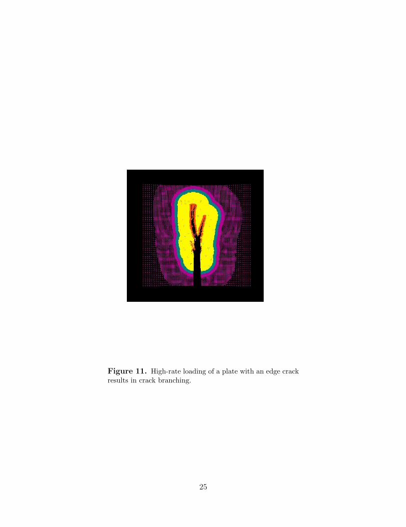
Figure 11. High-rate loading of a plate with an edge crackresults in crack branching.

25

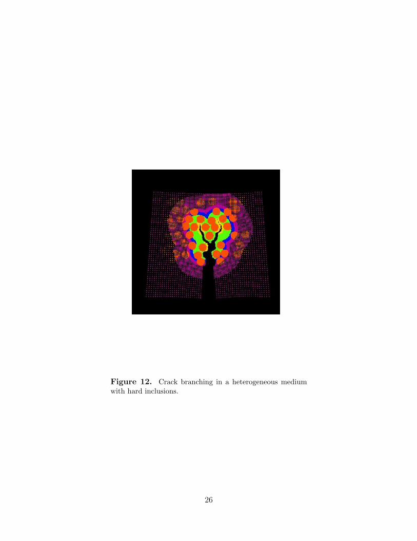
Figure 12. Crack branching in a heterogeneous mediumwith hard inclusions.

26

6 Discussion

The multiscale approach discussed in this report has the following advantages:

• The same equations are used at each level; only the value of the horizon changes.

• Levels interact only with the level immediately above and below.

• Each level solves only its own equation of motion. This is important because it avoidsthe difficulty of solving all the levels simultaneously.

• Each level uses its own time step. Higher levels use larger time steps than lower levels.In this sense, the method is multiscale in time as well as space.

• Small scale phenomena such as crack tip process zones can interact with larger scalestructural response. The computational cost of increasing the size of a structure beingmodeled is small, provided that most of it is in level L (thereby requiring only thecoarsest discretization.

The method has the disadvantage of involving computational complexity in programming thecommunications between levels, but this is perhaps true of all available multiscale techniques.Another disadvantage is that if there are many cracks that are widely distributed throughouta structure, the multiscale method treats nearly the whole body as level 0, negating anysavings in computational cost.

27

References

[1] S. A. Silling, Reformulation of elasticity theory for discontinuities and long-range forces,Journal of the Mechanics and Physics of Solids 48 (2000) 175–209.

[2] S. A. Silling and R. B. Lehoucq, Peridynamic theory of solid mechanics, Advances inApplied Mechanics 44 (2010) 73–168.

[3] S. A. Silling and E. Askari, A meshfree method based on the peridynamic model of solidmechanics, Computers and Structures 83 (2005) 1526–1535.

[4] B. L. Boyce, J. E. Bishop, A. Brown, T. Cordova, J.V. Cox, T.B. Crenshaw, K. Dion,J.M. Emery, J. T. Foster, J W. Foulk III, D. J. Littlewood, A. Mota, J. Ostien, S. Silling,B. W. Spencer, G. W. Wellman, Ductile failure X-prize, Sandia Report SAND2011-6801(2011).

[5] J. V. Cox, Selected preliminary results for the application of analytically enriched XFEMto problems with small cohesive zones, Sandia Technical Memorandum (2011).

[6] J. V. Cox, An extended finite element method with analytical enrichment for cohesivecrack modeling, International Journal for Numerical Methods in Engineering 78 (2009)48-83.

28

DISTRIBUTION:

1 MS 0899 Technical Library, 9536 (electronic copy)

29

30

v1.38