Hierarchical Bayesian Optimization Algorithm (hBOA)

Martin Pelikan

University of Missouri at St. Louis

pelikan@cs.umsl.edu

2

Foreword

Motivation• Black-box optimization (BBO) problem

• Set of all potential solutions

• Performance measure (evaluation procedure)

• Task: Find optimum (best solution)

• Formulation useful: No need for gradient, numerical functions, …

• But many important and tough challenges This talk

• Combine machine learning and evolutionary computation

• Create practical and powerful optimizers (BOA and hBOA)

3

Overview

Black-box optimization (BBO) BBO via probabilistic modeling

• Motivation and examples

• Bayesian optimization algorithm (BOA)

• Hierarchical BOA (hBOA)

Theory and experiment Conclusions

4

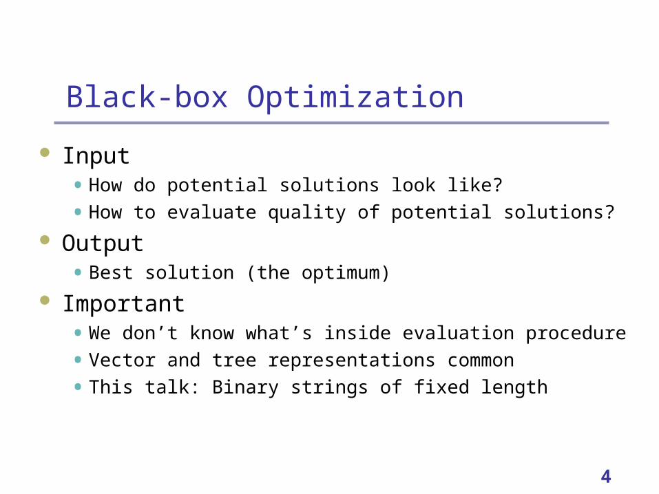
Black-box Optimization

Input• How do potential solutions look like?

• How to evaluate quality of potential solutions?

Output• Best solution (the optimum)

Important• We don’t know what’s inside evaluation procedure

• Vector and tree representations common

• This talk: Binary strings of fixed length

5

BBO: Examples

Atomic cluster optimization• Solutions: Vectors specifying positions of all atoms

• Performance: Lower energy is better

Telecom network optimization• Solutions: Connections between nodes (cities, …)

• Performance: Satisfy constraints, minimize cost

Design• Solutions: Vectors specifying parameters of the design

• Performance: Finite element analysis, experiment, …

6

BBO: Advantages & Difficulties

Advantages• Use same optimizer for all problems.

• No need for much prior knowledge. Difficulties

• Many places to go• 100-bit strings…1267650600228229401496703205376 solutions.

• Enumeration is not an option.

• Many places to get stuck• Local operators are not an option.

• Must learn what’s in the box automatically.

• Noise, multiple objectives, interactive evaluation, ...

7

Typical Black-Box Optimizer

Sample solutions Evaluated sampled solutions Learn to sample better

Sample Evaluate

Learn

8

Many Ways to Do It

Hill climber• Start with a random solution.

• Flip bit that improves the solution most.

• Finish when no more improvement possible. Simulated annealing

• Introduce Metropolis. Evolutionary algorithms

• Inspiration from natural evolution and genetics.

9

Evolutionary Algorithms

Evolve a population of candidate solutions. Start with a random population. Iteration

• SelectionSelect promising solutions

• VariationApply crossover and mutation to selected solutions

• ReplacementIncorporate new solutions into original population

10

Estimation of Distribution Algorithms

Replace standard variation operators by• Building a probabilistic model of promising

solutions

• Sampling the built model to generate new solutions

Probabilistic model• Stores features that make good solutions good

• Generates new solutions with just those features

11

EDAs

01011

11000

11001

10101

11001

10101

01011

11000

Selectedpopulation

Current population

Probabilistic

Model 11011

00111

01111

11001

Newpopulation

12

What Models to Use?

Our plan

• Simple example: Probability vector for binary strings

• Bayesian networks (BOA)

• Bayesian networks with local structures (hBOA)

13

Probability Vector

Baluja (1995) Assumes binary strings of fixed length Stores probability of a 1 in each position. New strings generated with those proportions. Example:

(0.5, 0.5, …, 0.5) for uniform distribution(1, 1, …, 1) for generating strings of all 1s

14

EDA Example: Probability Vector

01011

11000

11001

10101

11001

10101

01011

11000

Selectedpopulation

Current population

11101

11001

10101

10001

Newpopulation

11001

10101

01011

11000

1.0 0.5 0.5 0.0 1.0

15

Probability Vector Dynamics

Bits that perform better get more copies.And are combined in new ways.But context of each bit is ignored.Example problem 1: ONEMAX

Optimum: 111…1

∑=

=n

iin XXXXf

121 ),,,( K

16

Probability Vector on ONEMAX

0 10 20 30 40 500

0.1

0.2

0.3

0.4

0.5

0.6

0.7

0.8

0.9

1

Generation

Probability vector entries

Iteration

Pro

port

ion

s o

f 1s

Optimum

17

Probability Vector on ONEMAX

0 10 20 30 40 500

0.1

0.2

0.3

0.4

0.5

0.6

0.7

0.8

0.9

1

Generation

Probability vector entries

Iteration

Pro

port

ion

s o

f 1s

Optimum

Success

18

Probability Vector: Ideal Scale-up

O(n log n) evaluations until convergence• (Harik, Cantú-Paz, Goldberg, & Miller, 1997)

• (Mühlenbein, Schlierkamp-Vosen, 1993)

Other algorithms• Hill climber: O(n log n) (Mühlenbein, 1992)

• GA with uniform: approx. O(n log n)

• GA with one-point: slightly slower

19

When Does Prob. Vector Fail?

Example problem 2: Concatenated traps• Partition input string into disjoint groups of 5 bits.

• Each group contributes via trap (ones=num. ones):

• Concatenated trap = sum of single traps

• Optimum: 111…1

trap(ones) =5 if ones=54 −ones otherwise

⎧⎨⎩

20

Trap

0 1 2 3 4 5

0

1

2

3

4

5

Number of ones, u

trap(u)

Number of 1s

Tra

p

Globaloptimum

21

Probability Vector on Traps

0 10 20 30 40 500

0.1

0.2

0.3

0.4

0.5

0.6

0.7

0.8

0.9

1

Generation

Probability vector entries

Iteration

Pro

port

ion

s o

f 1s

Optimum

22

Probability Vector on Traps

0 10 20 30 40 500

0.1

0.2

0.3

0.4

0.5

0.6

0.7

0.8

0.9

1

Generation

Probability vector entries

Optimum

Failure

Iteration

Pro

port

ion

s o

f 1s

23

Why Failure?

Onemax: • Optimum in 111…1

• 1 outperforms 0 on average.

Traps: optimum in 11111, but• f(0****) = 2

• f(1****) = 1.375

So single bits are misleading.

24

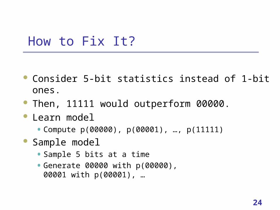
How to Fix It?

Consider 5-bit statistics instead of 1-bit ones. Then, 11111 would outperform 00000. Learn model

• Compute p(00000), p(00001), …, p(11111)

Sample model• Sample 5 bits at a time

• Generate 00000 with p(00000), 00001 with p(00001), …

25

Correct Model on Traps: Dynamics

0 10 20 30 40 500

0.1

0.2

0.3

0.4

0.5

0.6

0.7

0.8

0.9

1

Generation

Probabilities of 11111

Optimum

Iteration

Pro

port

ion

s o

f 1s

26

Correct Model on Traps: Dynamics

0 10 20 30 40 500

0.1

0.2

0.3

0.4

0.5

0.6

0.7

0.8

0.9

1

Generation

Probabilities of 11111

Optimum

Iteration

Pro

port

ion

s o

f 1s

Success

27

Good News: Good Stats Work Great!

Optimum in O(n log n) evaluations. Same performance as on onemax! Others

• Hill climber: O(n5 log n) = much worse.

• GA with uniform: O(2n) = intractable.

• GA with one point: O(2n) (without tight linkage).

28

Challenge

If we could learn and use context for each position• Find nonmisleading statistics.

• Use those statistics as in probability vector.

Then we could solve problems decomposable into statistics of order at most k with at most O(n2) evaluations!• And there are many of those problems.

29

Bayesian Optimization Algorithm (BOA)

Pelikan, Goldberg, & Cantú-Paz (1998) Use a Bayesian network (BN) as a model. Bayesian network

• Acyclic directed graph.

• Nodes are variables (string positions).

• Conditional dependencies (edges).

• Conditional independencies (implicit).

30

Conditional Dependency

X

ZY

X Y Z P(X | Y, Z)0 0 0 10%0 0 1 5%0 1 0 25%0 1 1 94%1 0 0 90%1 0 1 95%1 1 0 75%1 1 1 6%

31

Bayesian Network (BN)

Explicit: Conditional dependencies. Implicit: Conditional independencies. Probability tables

32

BOA

Current population

Selectedpopulation

New population

Bayesian network

33

BOA Variation

Two steps• Learn a Bayesian network (for promising solutions)

• Sample the built Bayesian network (to generate new candidate solutions)

Next• Brief look at the two steps in BOA

34

Learning BNs

Two components:

• Scoring metric (to evaluate models).

• Search procedure (to find the best model).

35

Learning BNs: Scoring Metrics

Bayesian metrics• Bayesian-Dirichlet with likelihood equivalence

Minimum description length metrics• Bayesian information criterion (BIC)

BD(B) =p(B)Γ(m'(π i ))

Γ(m'(π i ) + m(π i ))Γ(m'(xi ,π i ) + m(xi ,π i ))

Γ(m'(xi ,π i ))xi

∏π

i

∏i=1

n

∏

BIC(B) = −H(Xi |Πi )N −2Πi

log2 N2

⎛

⎝⎜⎞

⎠⎟i=1

n

∑

36

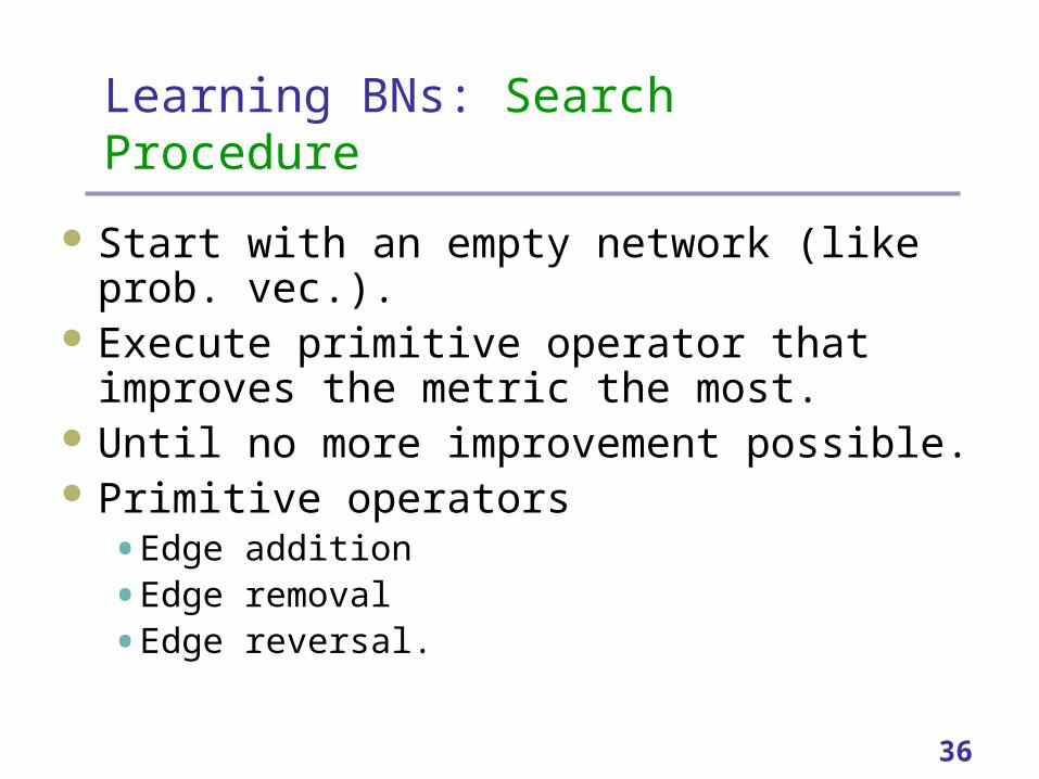
Learning BNs: Search Procedure

Start with an empty network (like prob. vec.). Execute primitive operator that improves the

metric the most. Until no more improvement possible. Primitive operators

• Edge addition

• Edge removal

• Edge reversal.

37

Sampling BNs: PLS

Probabilistic logic sampling (PLS) Two phases

• Create ancestral ordering of variables:Each variable depends only on predecessors

• Sample all variables in that order using CPTs:Repeat for each new candidate solution

38

BOA Theory: Key Components

Primary target: Scalability Population sizing N

• How large populations for reliable solution?

Number of generations (iterations) G• How many iterations until convergence?

Overall complexity• O(N x G)

• Overhead: Low-order polynomial in N, G, and n.

39

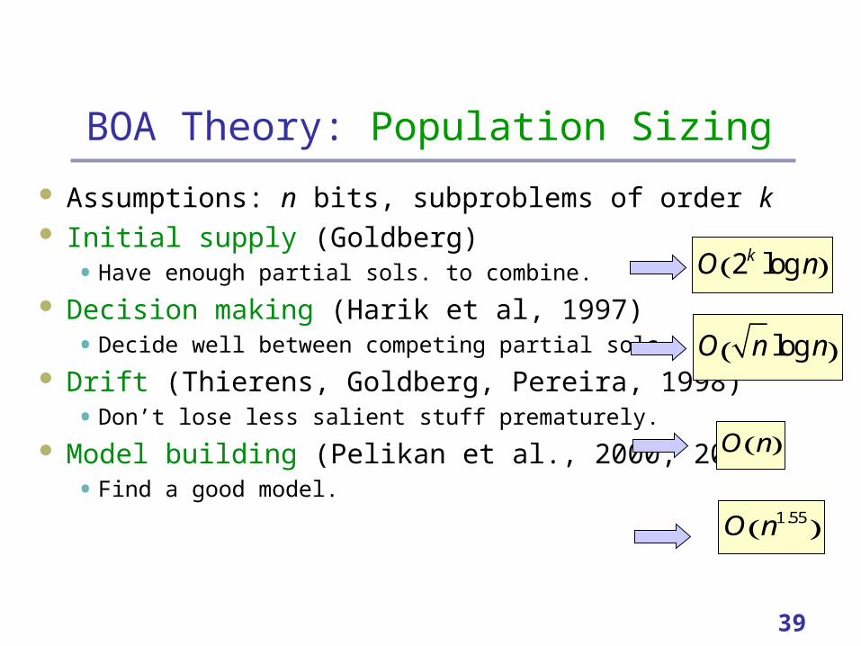
BOA Theory: Population Sizing

Assumptions: n bits, subproblems of order k Initial supply (Goldberg)

• Have enough partial sols. to combine.

Decision making (Harik et al, 1997)• Decide well between competing partial sols.

Drift (Thierens, Goldberg, Pereira, 1998)• Don’t lose less salient stuff prematurely.

Model building (Pelikan et al., 2000, 2002)• Find a good model.

O n( )

O n1.55( )

O n log n( )

O 2k log n( )

40

BOA Theory: Num. of Generations

Two bounding cases Uniform scaling

• Subproblems converge in parallel

• Onemax model (Muehlenbein & Schlierkamp-Voosen, 1993)

Exponential scaling• Subproblems converge sequentially

• Domino convergence (Thierens, Goldberg, Pereira, 1998)

O n( )

O n( )

41

Theory• Population sizing (Pelikan et al., 2000, 2002)

1. Initial supply.2. Decision making.3. Drift.4. Model building.

• Iterations until convergence (Pelikan et al., 2000, 2002)1. Uniform scaling.2. Exponential scaling.

BOA solves order-k decomposable problems in O(n1.55) to O(n2) evaluations!

Good News

O(n) to O(n1.05)

O(n0.5) to O(n)

42

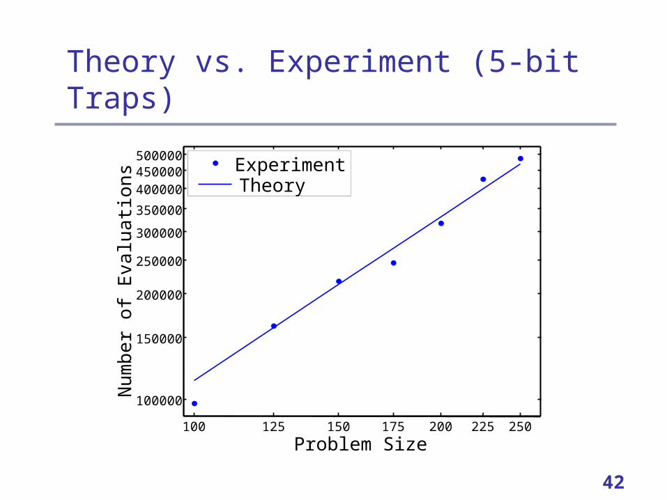
Theory vs. Experiment (5-bit Traps)

100 125 150 175 200 225 250

100000

150000

200000

250000

300000

350000

400000450000500000

Problem Size

Nu

mb

er

of E

valu

atio

ns

ExperimentTheory

43

Additional Plus: Prior Knowledge

BOA need not know much about problem• Only set of solutions + measure (BBO).

BOA can use prior knowledge• High-quality partial or full solutions.

• Likely or known interactions.

• Previously learned structures.

• Problem specific heuristics, search methods.

44

From Single Level to Hierarchy

What if problem can’t be decomposed like this? Inspiration from human problem solving. Use hierarchical decomposition

• Decompose problem on multiple levels.

• Solutions from lower levels = basic building blocks for constructing solutions on the current level.

• Bottom-up hierarchical problem solving.

45

Hierarchical Decomposition

Car

Engine Braking system Electrical system

Fuel system Valves Ignition system

46

3 Keys to Hierarchy Success

Proper decomposition• Must decompose problem on each level properly.

Chunking• Must represent & manipulate large order solutions.

Preservation of alternative solutions• Must preserve alternative partial solutions (chunks).

47

Hierarchical BOA (hBOA)

Pelikan & Goldberg (2001) Proper decomposition

• Use BNs as BOA.

Chunking• Use local structures in BNs.

Preservation of alternative solutions• Restricted tournament replacement (niching).

48

Local Structures in BNs

Look at one conditional dependency.• 2k probabilities for k parents.

Why not use more powerful representationsfor conditional probabilities?

X1

X3X2

X2X3 P(X1=0|X2X3)

00 26 %

01 44 %

10 15 %

11 15 %

49

Local Structures in BNs

Look at one conditional dependency.• 2k probabilities for k parents.

Why not use more powerful representationsfor conditional probabilities?

X1

X3X2

X2

X3

0 1

0 1

26% 44%

15%

50

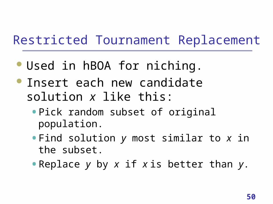
Restricted Tournament Replacement

Used in hBOA for niching. Insert each new candidate solution x like this:

• Pick random subset of original population.

• Find solution y most similar to x in the subset.

• Replace y by x if x is better than y.

51

hBOA: Scalability

Solves nearly decomposable and hierarchical problems (Simon, 1968)

Number of evaluations grows as a low-order polynomial

Most other methods fail to solve many such problems

52

Hierarchical Traps

Traps on multiple levels. Blocks of 0s and 1s mapped

to form solutions on thenext level.

3 challenges• Many local optima

• Deception everywhere

• No single-level decomposability

000 111

000

000 000111 111

53

Hierarchical Traps

27 81 243 729

104

105

106

Problem Size

Number of Evaluations

hBOA

O(n1.63 log(n))

54

Other Similar Algorithms Estimation of distribution algorithms (EDAs)

• Dynamic branch of evolutionary computation Examples:

• PBIL (Baluja, 1995)• Univariate distributions (full independence)

• COMIT• Considers tree models

• ECGA• Groups of variables considered together

• EBNA (Etxeberria et al., 1999), LFDA (Muhlenbein et al., 1999)• Versions of BOA

• And others…

55

EDAs: Promising Results

Artificial classes of problems MAXSAT, SAT (Pelikan, 2005). Nurse scheduling (Li, Aickelin, 2003) Military antenna design (Santarelli et al., 2004) Groundwater remediation design (Arst et al., 2004) Forest management (Ducheyne et al., 2003) Telecommunication network design (Rothlauf, 2002) Graph partitioning (Ocenasek, Schwarz, 1999; Muehlenbein,

Mahnig, 2002; Baluja, 2004) Portfolio management (Lipinski, 2005) Quantum excitation chemistry (Sastry et al., 2005)

56

Current Projects

Algorithm design• hBOA for computer programs.

• hBOA for geometries (distance/angle-based).

• hBOA for machine learners and data miners.

• hBOA for scheduling and permutation problems.

• Efficiency enhancement for EDAs.

• Multiobjective EDAs. Applications

• Cluster optimization and spin glasses.

• Data mining.

• Learning classifier systems & neural networks.

57

Conclusions for Researchers

Principled design of practical BBOers:• Scalability

• Robustness

• Solution to broad classes of problems

Facetwise design and little models• Useful for approaching research in evol. comp.

• Allow creation of practical algorithms & theory

58

Conclusions for Practitioners

BOA and hBOA revolutionary optimizers• Need no parameters to tune.

• Need almost no problem specific knowledge.

• But can incorporate knowledge in many forms.

• Problem regularities discovered and exploited automatically.

• Solves broad classes of challenging problems.

• Even problems unsolvable by any other BBOer.

• Can deal with noise & multiple objectives.

59

Book on hBOA

Martin Pelikan (2005)

Hierarchical Bayesian optimization algorithm:

Toward a new generation of evolutionary algorithms

Springer

60

Contact

Martin PelikanDept. of Math. and Computer Science, 320 CCBUniversity of Missouri at St. Louis8001 Natural Bridge Rd.St. Louis, MO 63121

pelikan@cs.umsl.eduhttp://www.cs.umsl.edu/~pelikan/

61

Problem 1: Concatenated Traps

Partition input binary strings into 5-bit groups.

Partitions fixed but uknown. Each partition contributes

the same. Contributions sum up.

0 1 2 3 4 5

0

1

2

3

4

5

Number of ones, u

trap(u)

62

Concatenated 5-bit Traps

100 125 150 175 200 225 250

100000

150000

200000

250000

300000

350000

400000450000500000

Problem Size

Nu

mb

er

of E

valu

atio

ns

ExperimentTheory

63

Spin Glasses: Problem Definition

1D, 2D, or 3D grid of spins. Each spin can take values +1 or -1. Relationships between neighboring spins (i,j) are

defined by coupling constants Ji,j. Usually periodic boundary conditions (toroid). Task: Find values of spins to minimize the energy

∑=ji

jjii sJsE,

,

64

Spin Glasses as Constraint Satisfaction

==

=

=

≠

≠

≠

≠

≠≠

≠

≠

Spins:

≠ =Constraints:

65

Spin Glasses: Problem Difficulty 1D – Easy, set spins sequentially. 2D – Several polynomial methods exist, best is

• Exponentially many local optima

• Standard approaches (e.g. simulated annealing, MCMC) fail 3D – NP-complete, even for couplings {-1,0,+1}. Often random subclasses are considered

• +-J spin glasses: Couplings uniform -1 or +1

• Gaussian spin glasses: Couplings N(0, 2).

O n3.5( )

66

Ising Spin Glasses (2D)

64 100 144 196 256 324 400

103

Problem Size

Number of Evaluations

hBOA

O(n1.51)

67

Results on 2D Spin Glasses

Number of evaluations is O(n1.51). Overall time is O(n3.51). Compare O(n3.51) to O(n3.5) for best method

(Galluccio & Loebl, 1999) Great also on Gaussians.

68

Ising Spin Glasses (3D)

64 125 216 34310

3

104

105

106

Problem Size

Number of Evaluations

Experimental average

O(n3.63 )

69

MAXSAT

Given a CNF formula. Find interpretation of Boolean variables that

maximizes the number of satisfied clauses.

(x2 x7 x5 ) (x1 x4 x3)

70

MAXSAT Difficulty

MAXSAT is NP complete for k-CNF, k>1

But “random” problems are rather easy for almost any method.

Many interesting subclasses on SATLIB, e.g.• 3-CNF from phase transition ( c = 4.3 n )

• CNFs from other problems (graph coloring, …)

71

MAXSAT: Random 3CNFs

72

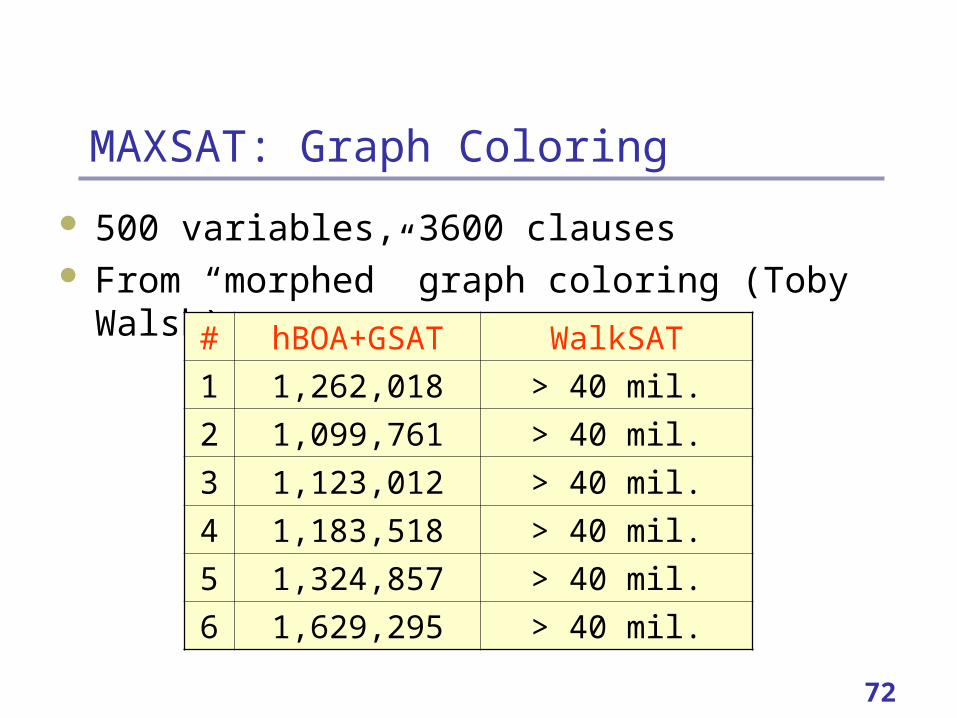
MAXSAT: Graph Coloring

500 variables, 3600 clauses From “morphed” graph coloring (Toby Walsh)

# hBOA+GSAT WalkSAT

1 1,262,018 > 40 mil.

2 1,099,761 > 40 mil.

3 1,123,012 > 40 mil.

4 1,183,518 > 40 mil.

5 1,324,857 > 40 mil.

6 1,629,295 > 40 mil.

73

Spin Glass to MAXSAT

Convert each coupling Jij with spins si and sj:

Jij =+1 (si sj) (si sj)

Jij = -1 (si sj) (si sj) Consistent pairs of spins = 2 sat. clauses Inconsistent pairs of spins = 1 sat. clause MAXSAT solvers perform poorly even in 2D!