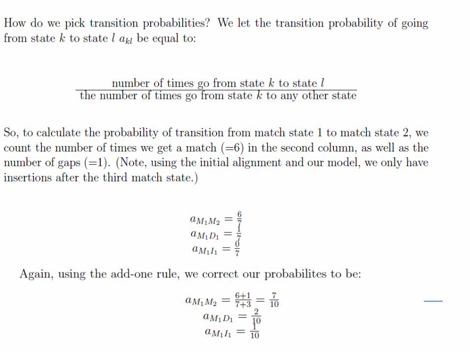
Hidden Markov Model

CG-Islands

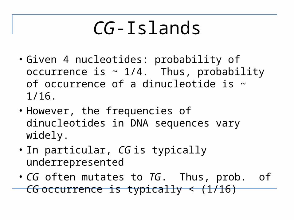
• Given 4 nucleotides: probability of occurrence is ~ 1/4. Thus, probability of occurrence of a dinucleotide is ~ 1/16.

• However, the frequencies of dinucleotides in DNA sequences vary widely.

• In particular, CG is typically underrepresented• CG often mutates to TG. Thus, prob. of CG

occurrence is typically < (1/16)

Why CG-Islands?

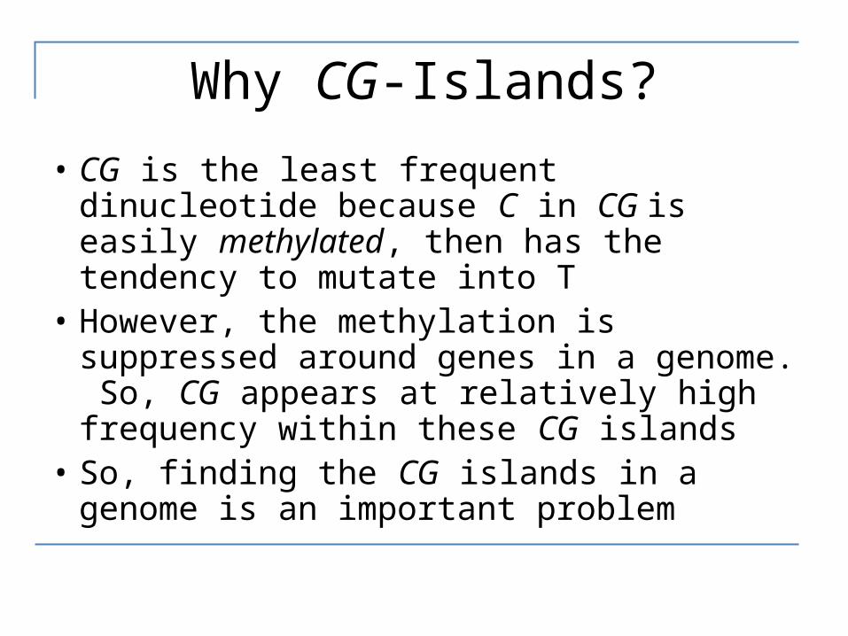
• CG is the least frequent dinucleotide because C in CG is easily methylated, then has the tendency to mutate into T

• However, the methylation is suppressed around genes in a genome. So, CG appears at relatively high frequency within these CG islands

• So, finding the CG islands in a genome is an important problem

CG Islands and the “Fair Bet Casino”

• The CG islands problem can be modeled after a problem named “The Fair Bet Casino”

• The game is to flip coins, which results in only two possible outcomes: Head or Tail.

• The Fair coin will give Heads and Tails with same probability ½.

• The Biased coin will give Heads with prob. ¾.

The “Fair Bet Casino” (cont’d)

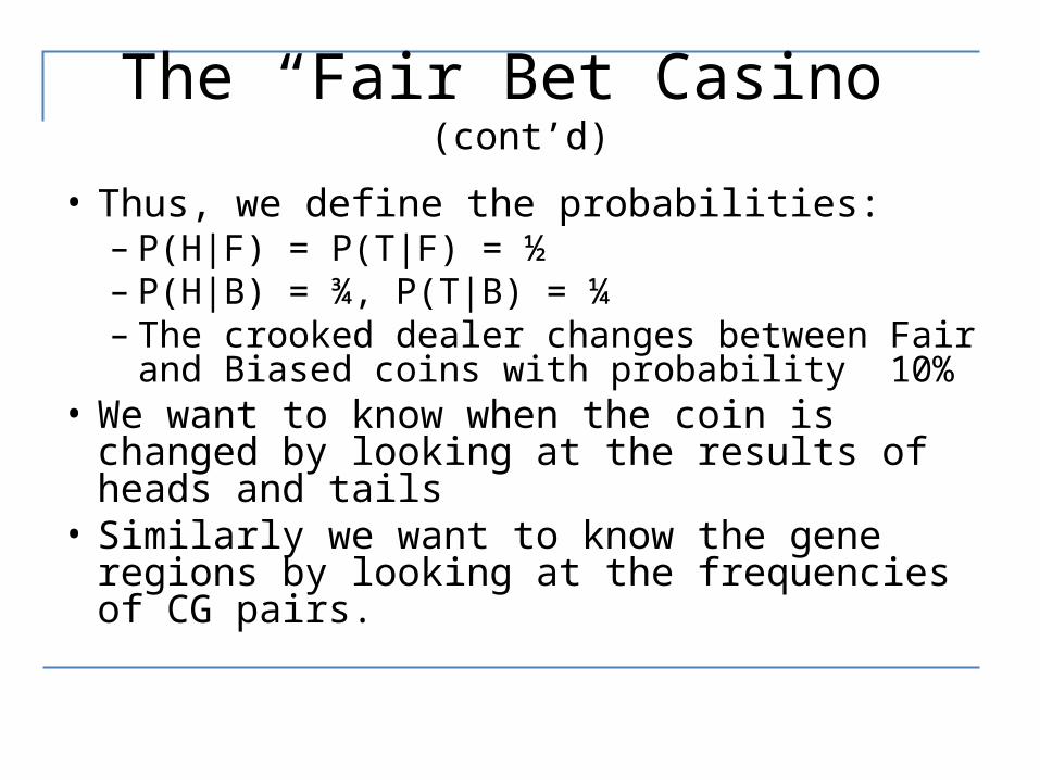
• Thus, we define the probabilities:– P(H|F) = P(T|F) = ½– P(H|B) = ¾, P(T|B) = ¼– The crooked dealer changes between Fair and

Biased coins with probability 10%• We want to know when the coin is changed by

looking at the results of heads and tails• Similarly we want to know the gene regions by

looking at the frequencies of CG pairs.

The Fair Bet Casino Problem

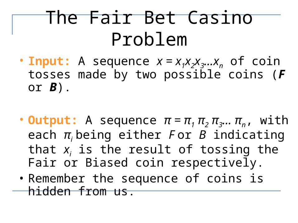
• Input: A sequence x = x1x2x3…xn of coin tosses made by two possible coins (F or B).

• Output: A sequence π = π1 π2 π3… πn, with each

πi being either F or B indicating that xi is the result of tossing the Fair or Biased coin respectively.

• Remember the sequence of coins is hidden from us.

Problem…

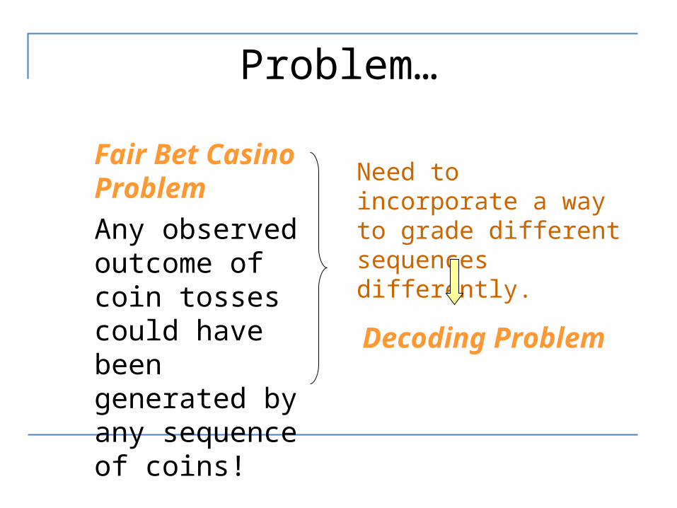
Fair Bet Casino ProblemAny observed outcome of coin tosses could have been generated by any sequence of coins!

Need to incorporate a way to grade different sequences differently.

Decoding Problem

P(x|fair coin) vs. P(x|biased coin)

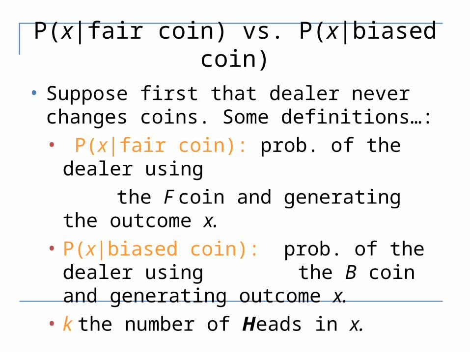
• Suppose first that dealer never changes coins. Some definitions…:• P(x|fair coin): prob. of the dealer using the F coin and generating the outcome x.• P(x|biased coin): prob. of the dealer using

the B coin and generating outcome x.• k the number of Heads in x.

P(x|fair coin) vs. P(x|biased coin)

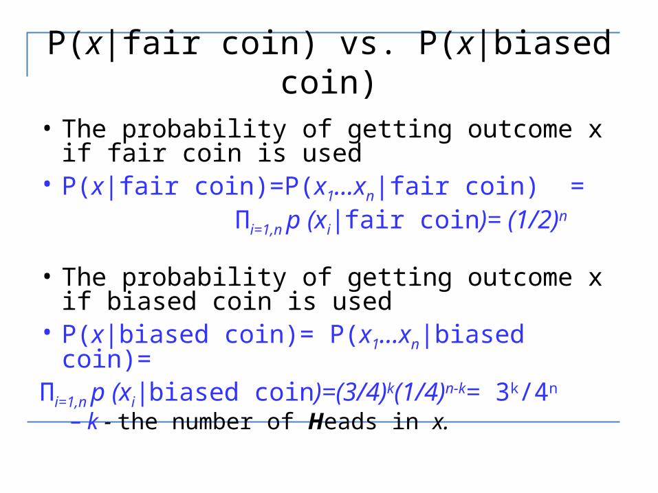
• The probability of getting outcome x if fair coin is used

• P(x|fair coin)=P(x1…xn|fair coin) = Πi=1,n p (xi|fair coin)= (1/2)n

• The probability of getting outcome x if biased coin is used

• P(x|biased coin)= P(x1…xn|biased coin)=Πi=1,n p (xi|biased coin)=(3/4)k(1/4)n-k= 3k/4n

– k - the number of Heads in x.

Log-odds Ratio

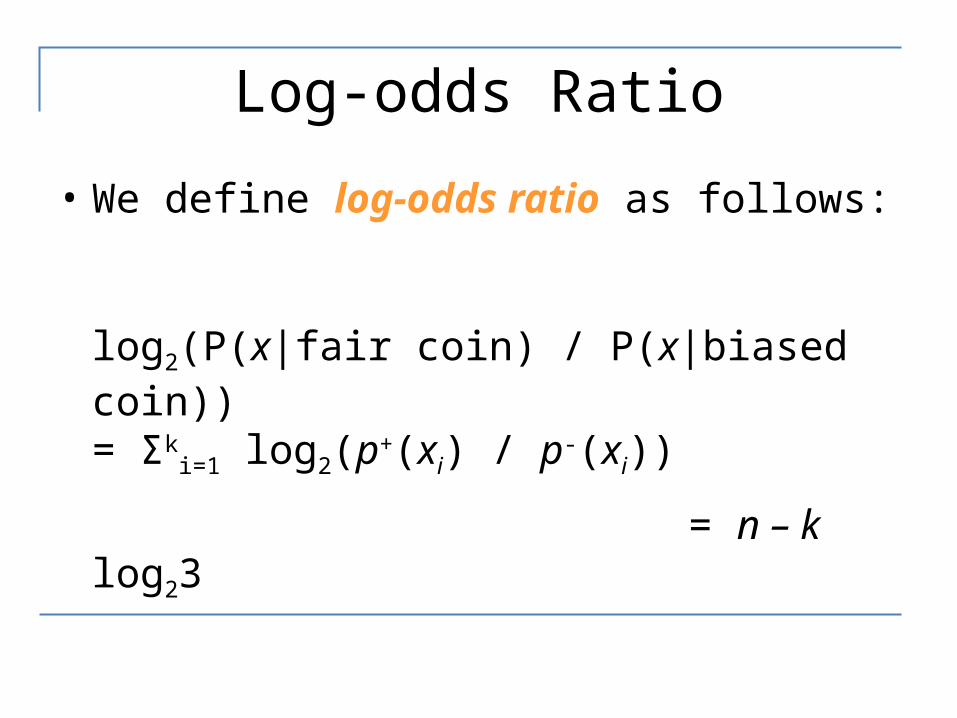
• We define log-odds ratio as follows:

log2(P(x|fair coin) / P(x|biased coin)) = Σk

i=1 log2(p+(xi) / p-(xi))

= n – k log23

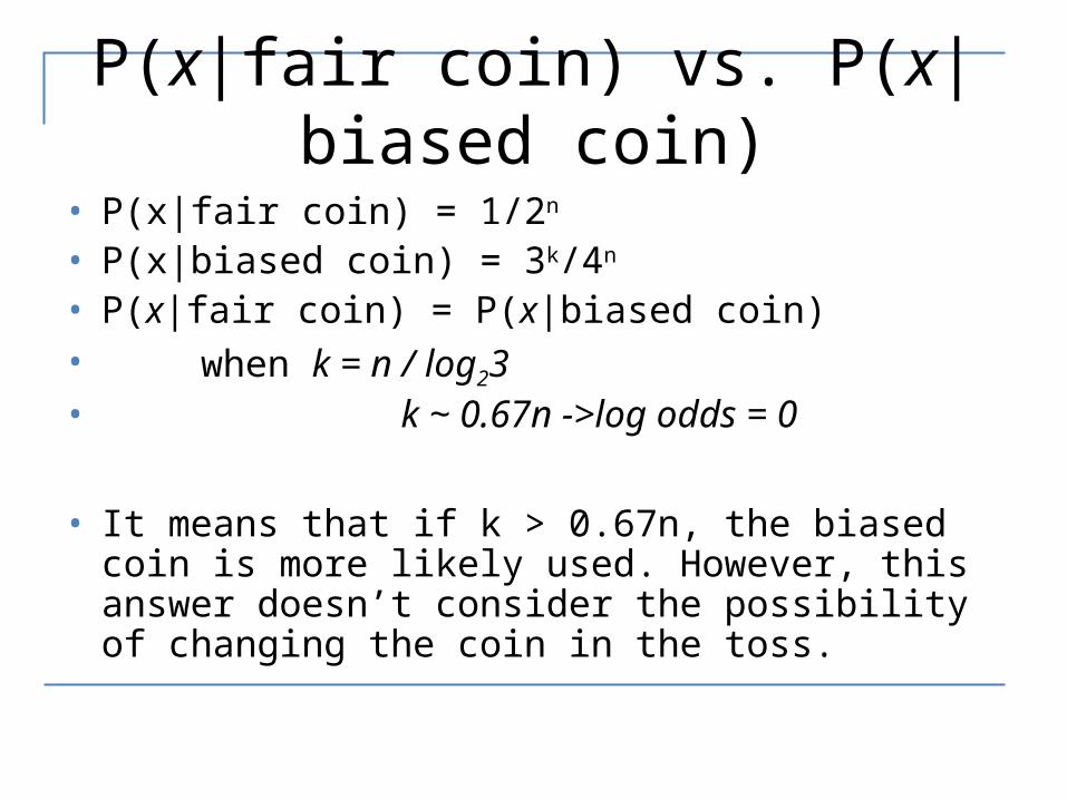
P(x|fair coin) vs. P(x|biased coin)• P(x|fair coin) = 1/2n

• P(x|biased coin) = 3k/4n • P(x|fair coin) = P(x|biased coin)• when k = n / log23 • k ~ 0.67n ->log odds = 0

• It means that if k > 0.67n, the biased coin is more likely used. However, this answer doesn’t consider the possibility of changing the coin in the toss.

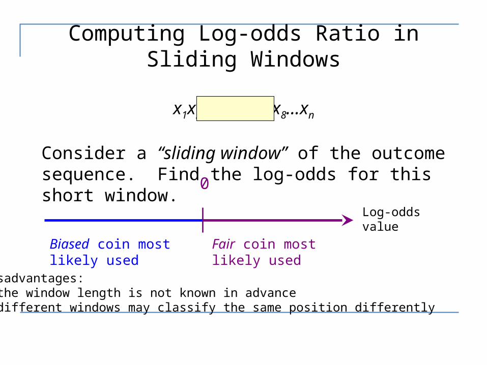
Computing Log-odds Ratio in Sliding Windows

x1x2x3x4x5x6x7x8…xn

Consider a “sliding window” of the outcome sequence. Find the log-odds for this short window.

Log-odds value

0

Fair coin most likely used

Biased coin most likely used

Disadvantages:- the window length is not known in advance- different windows may classify the same position differently

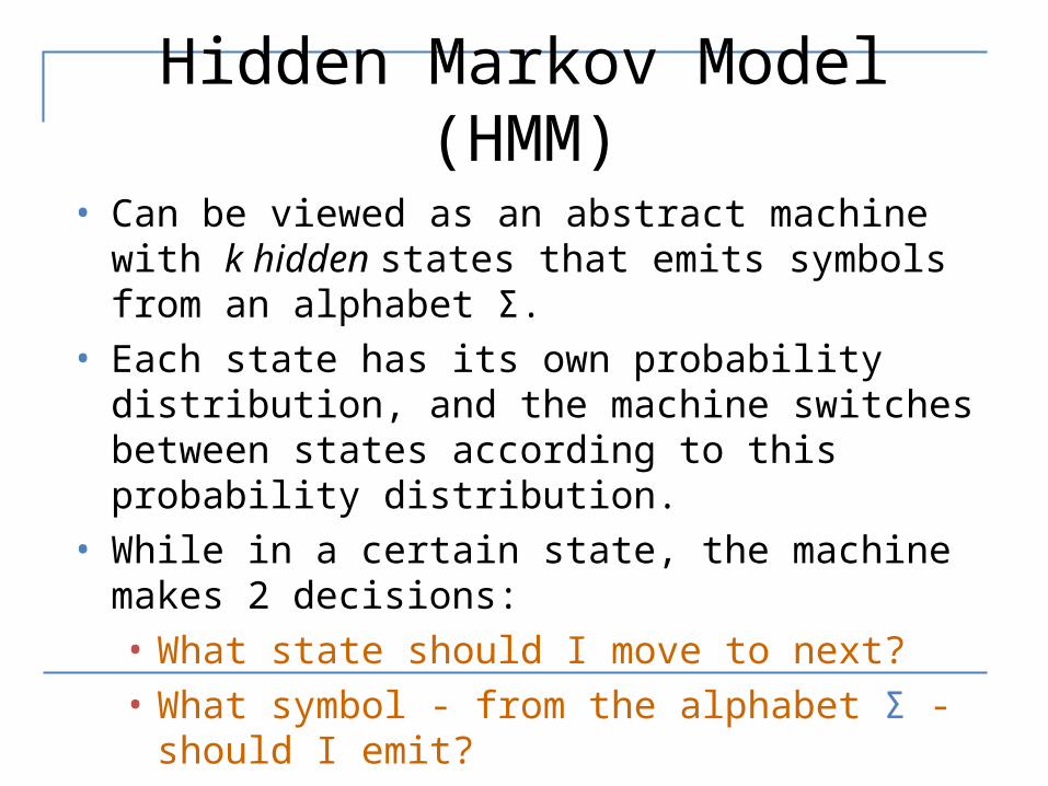
Hidden Markov Model (HMM)

• Can be viewed as an abstract machine with k hidden states that emits symbols from an alphabet Σ.

• Each state has its own probability distribution, and the machine switches between states according to this probability distribution.

• While in a certain state, the machine makes 2 decisions:• What state should I move to next?• What symbol - from the alphabet Σ - should I emit?

Why “Hidden”?

• Observers can see the emitted symbols of an HMM but have no ability to know which state the HMM is currently in.

• Thus, the goal is to infer the most likely hidden states of an HMM based on the given sequence of emitted symbols.

HMM Parameters

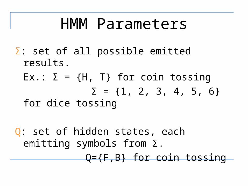
Σ: set of all possible emitted results.Ex.: Σ = {H, T} for coin tossing

Σ = {1, 2, 3, 4, 5, 6} for dice tossing

Q: set of hidden states, each emitting symbols from Σ.

Q={F,B} for coin tossing

HMM Parameters (cont’d)

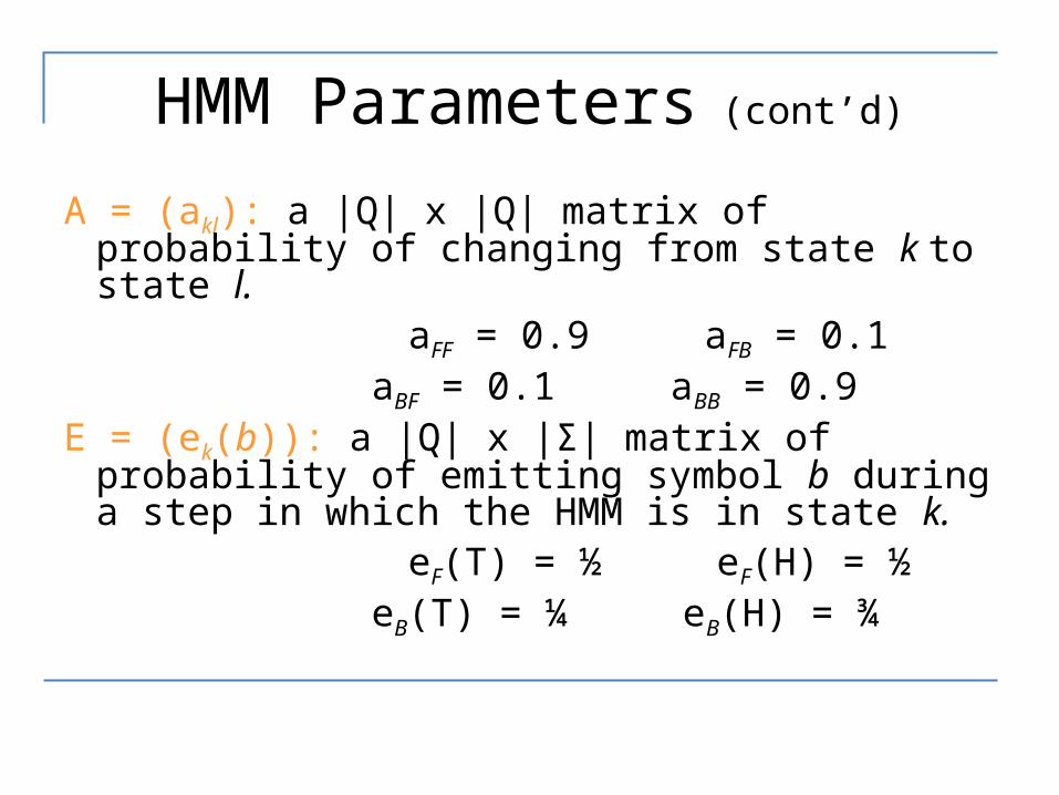
A = (akl): a |Q| x |Q| matrix of probability of changing from state k to state l.

aFF = 0.9 aFB = 0.1 aBF = 0.1 aBB = 0.9

E = (ek(b)): a |Q| x |Σ| matrix of probability of emitting symbol b during a step in which the HMM is in state k.

eF(T) = ½ eF(H) = ½ eB(T) = ¼ eB(H) = ¾

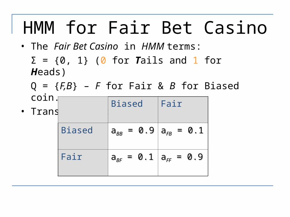
HMM for Fair Bet Casino• The Fair Bet Casino in HMM terms:

Σ = {0, 1} (0 for Tails and 1 for Heads)Q = {F,B} – F for Fair & B for Biased coin.

• Transition Probabilities A

Biased Fair

Biased aaBBBB = 0.9 = 0.9 aaFBFB = 0.1 = 0.1

Fair aaBFBF = 0.1 = 0.1 aaFFFF = 0.9 = 0.9

HMM for Fair Bet Casino (cont’d)

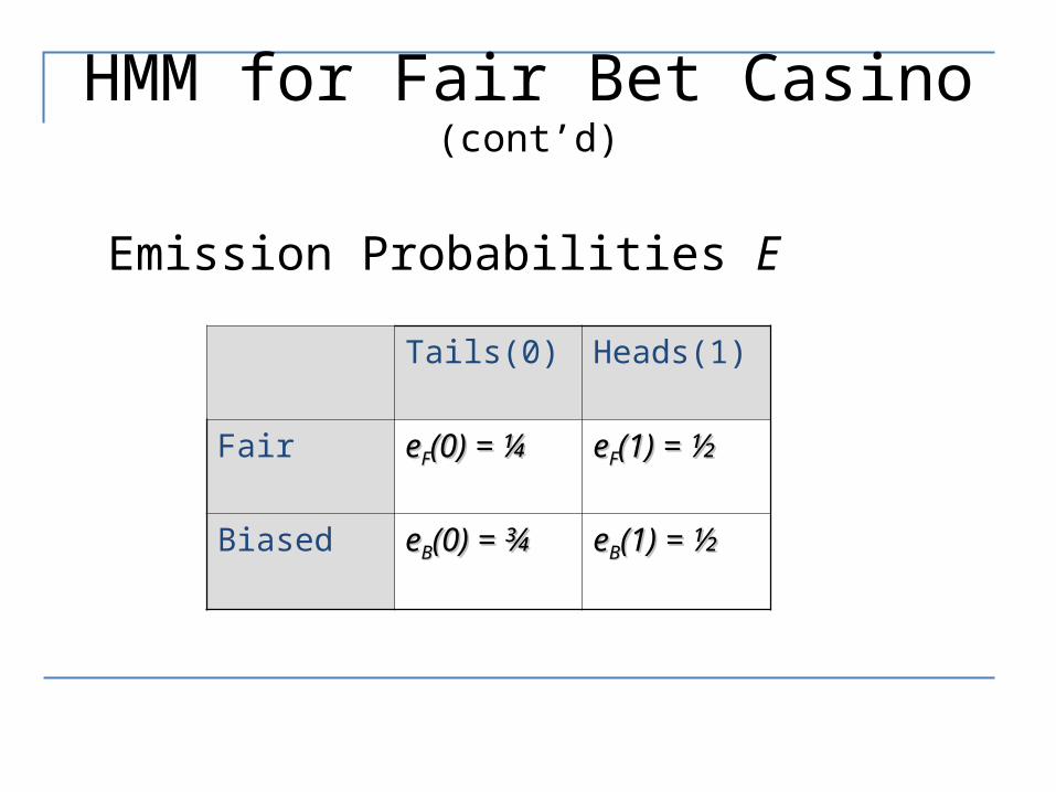
Emission Probabilities E

Tails(0) Heads(1)

Fair eeFF(0) = ¼(0) = ¼ eeFF(1) = ½(1) = ½

Biased eeBB(0) = ¾(0) = ¾ eeBB(1) = ½(1) = ½

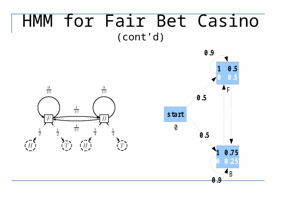
HMM for Fair Bet Casino (cont’d)

start

0

1 0.50 0.5

1 0.750 0.25

F

B

0.1 0.1

0.5

0.5

0.9

0.9

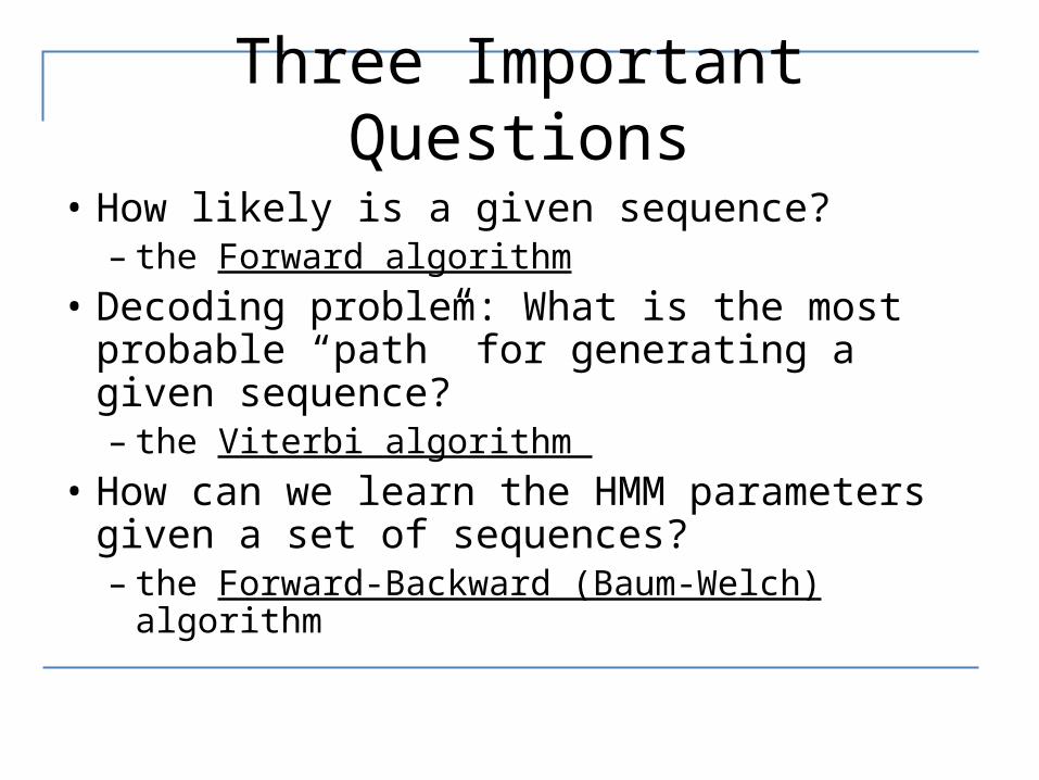
Three Important Questions

• How likely is a given sequence?– the Forward algorithm

• Decoding problem: What is the most probable “path” for generating a given sequence?– the Viterbi algorithm

• How can we learn the HMM parameters given a set of sequences?– the Forward-Backward (Baum-Welch) algorithm

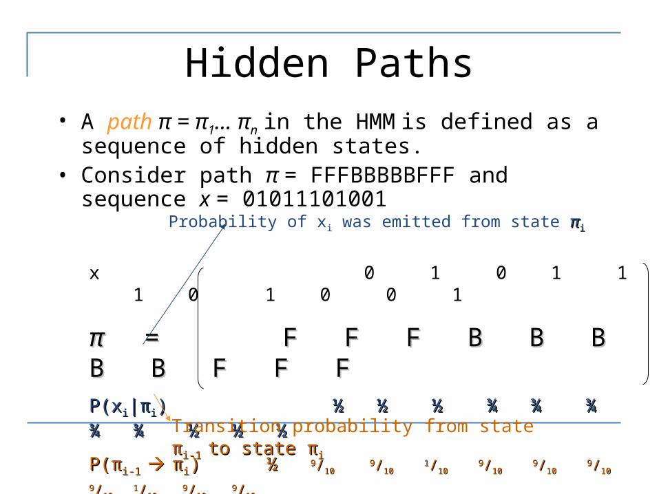
Hidden Paths• A path π = π1… πn in the HMM is defined as a sequence of

hidden states.• Consider path π = FFFBBBBBFFF and sequence x =

01011101001

x 0 1 0 1 1 1 0 1 0 0 1

π π = F F F B B B B B F F = F F F B B B B B F F FFP(xP(xii|π|πii)) ½ ½ ½ ¾ ¾ ¾ ¾ ¾ ½ ½ ½ ½ ½ ½ ¾ ¾ ¾ ¾ ¾ ½ ½ ½

P(πP(πi-1 i-1 ππii)) ½ ½ 99//1010 99//10 10 11//10 10

99//10 10 99//10 10

99//10 10 99//10 10

11//10 10 99//10 10

99//1010 Transition probability from state ππi-1 i-1 to to state πstate πii

Probability of xi was emitted from state ππii

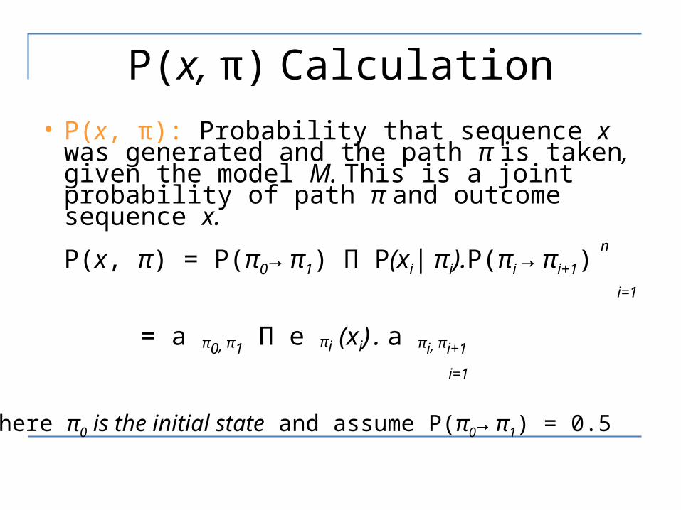
P(x, π) Calculation• P(x, π): Probability that sequence x was

generated and the path π is taken, given the model M. This is a joint probability of path π and outcome sequence x. n P(x, π) = P(π0→ π1) Π P(xi| πi).P(πi → πi+1)

i=1

= a π0, π1 Π e πi (xi) . a πi, πi+1 i=1

Where π0 is the initial state and assume P(π0→ π1) = 0.5

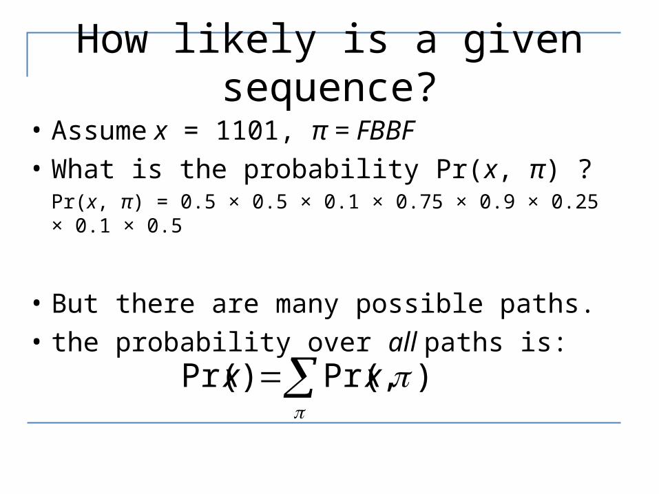
How likely is a given sequence?

• Assume x = 1101, π = FBBF• What is the probability Pr(x, π) ?

Pr(x, π) = 0.5 × 0.5 × 0.1 × 0.75 × 0.9 × 0.25 × 0.1 × 0.5

• But there are many possible paths.• the probability over all paths is:

),Pr()Pr( xx

How Likely is a Given Sequence?

• It is not practical to sum up all possible paths. • The Forward algorithm enables us to compute

this efficiently• Defined fk,i (forward probability) as the

probability of emitting the prefix x1…xi and being the state π = k.

Pr(x1…xi, πi = k)

• fk,i can be computed with a recurrence relation.

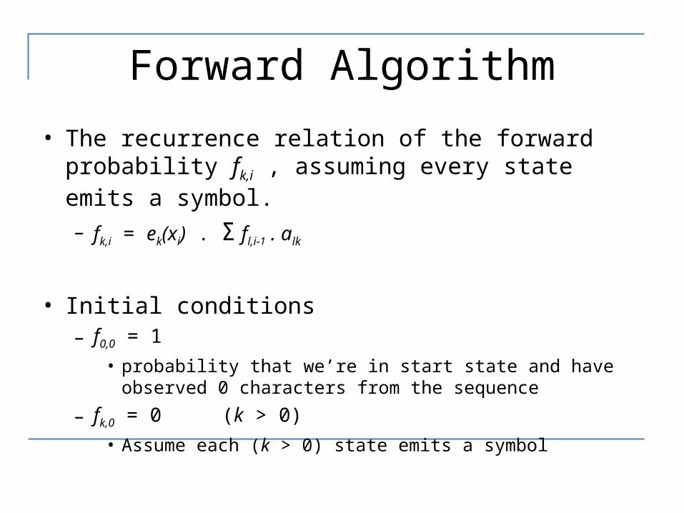
Forward Algorithm

• The recurrence relation of the forward probability fk,i , assuming every state emits a symbol.– fk,i = ek(xi) . Σ fl,i-1 . alk

• Initial conditions– f0,0 = 1

• probability that we’re in start state and have observed 0 characters from the sequence

– fk,0 = 0 (k > 0)• Assume each (k > 0) state emits a symbol

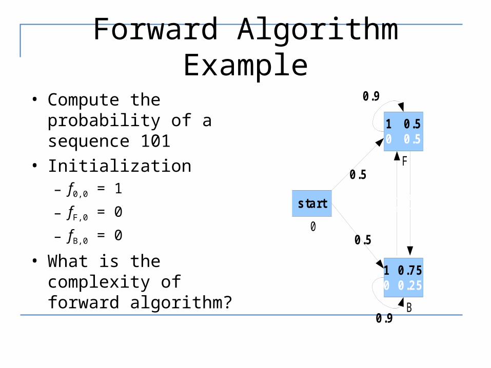
Forward Algorithm Example

• Compute the probability of a sequence 101

• Initialization– f0,0 = 1

– fF,0 = 0

– fB,0 = 0

• What is the complexity of forward algorithm?

start

0

1 0.50 0.5

1 0.750 0.25

F

B

0.1 0.1

0.5

0.5

0.9

0.9

Forward Algorithm Example

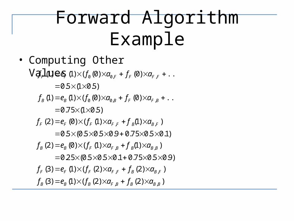
• Computing Other Values

))2()2(()1()3(

))2()2(()1()3(

)9.05.075.01.05.05.0(25.0

))1()1(()0()2(

)1.05.075.09.05.05.0(5.0

))1()1(()0()2(

)5.01(75.0

...))0()0(()1()1(

)5.01(5.0

...))0()0(()1()1(

,,

,,

,,

,,

,,00

,,00

BBBBFBBB

FBBFFFFF

BBBBFFBB

FBBFFFFF

BFFBBB

FFFFFF

afafef

afafef

afafef

afafef

afafef

afafef

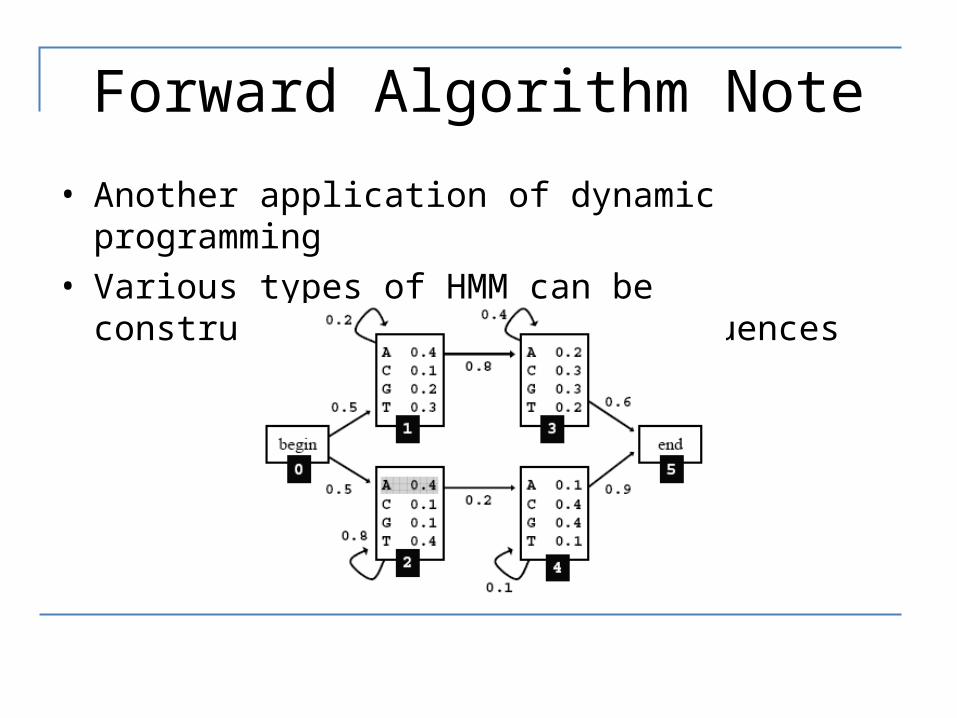
Forward Algorithm Note

• Another application of dynamic programming• Various types of HMM can be constructed for biological

sequences

Decoding Problem

• Goal: Find an optimal hidden path of states given observations.

• Input: Sequence of observations x = x1…xn generated by an HMM M(Σ, Q, A, E)

• Output: A hidden path that maximizes P(x, π) over all possible paths π.

Viterbi Algorithm• Andrew Viterbi used a edit graph to solve the Decoding

Problem.– n layers and Q states in each layer – Every choice of π = π1… πn corresponds to a path in the

graph.• The only valid direction in the graph is eastward.• This graph has |Q|2(n-1) edges.

– Q is the number of states• The decoding problem is to reduced to finding the

most probable path in the edit graph.

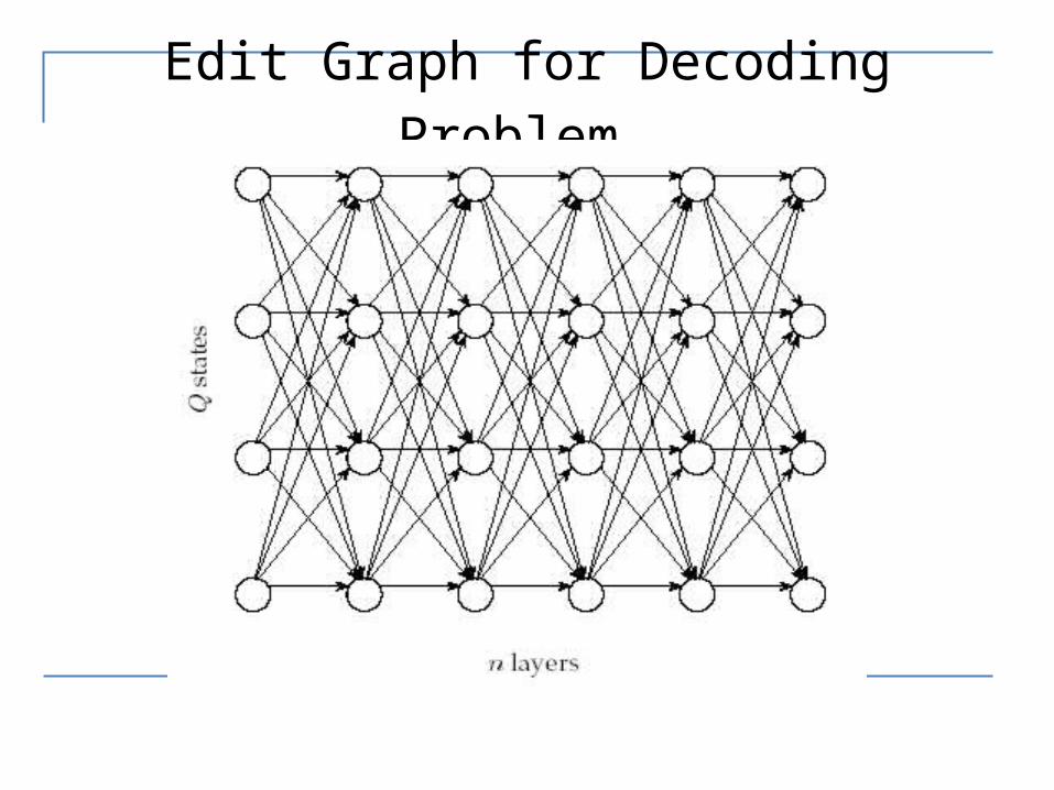
Edit Graph for Decoding Problem

Decoding Problem (cont’d)

• Every path in the graph has the probability P(x, π).

• The Viterbi algorithm finds the path that maximizes P(x, π) among all possible paths.

• Again we cannot check every path naively, but we can again use recurrence relation and dynamic programming

Decoding Problem (cont’d)

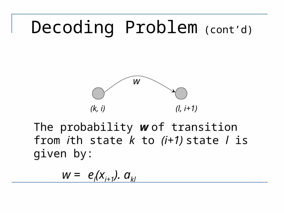
w

The probability w of transition from ith state k to (i+1) state l is given by:

w = el(xi+1). akl

(k, i) (l, i+1)

Recurrence Relation

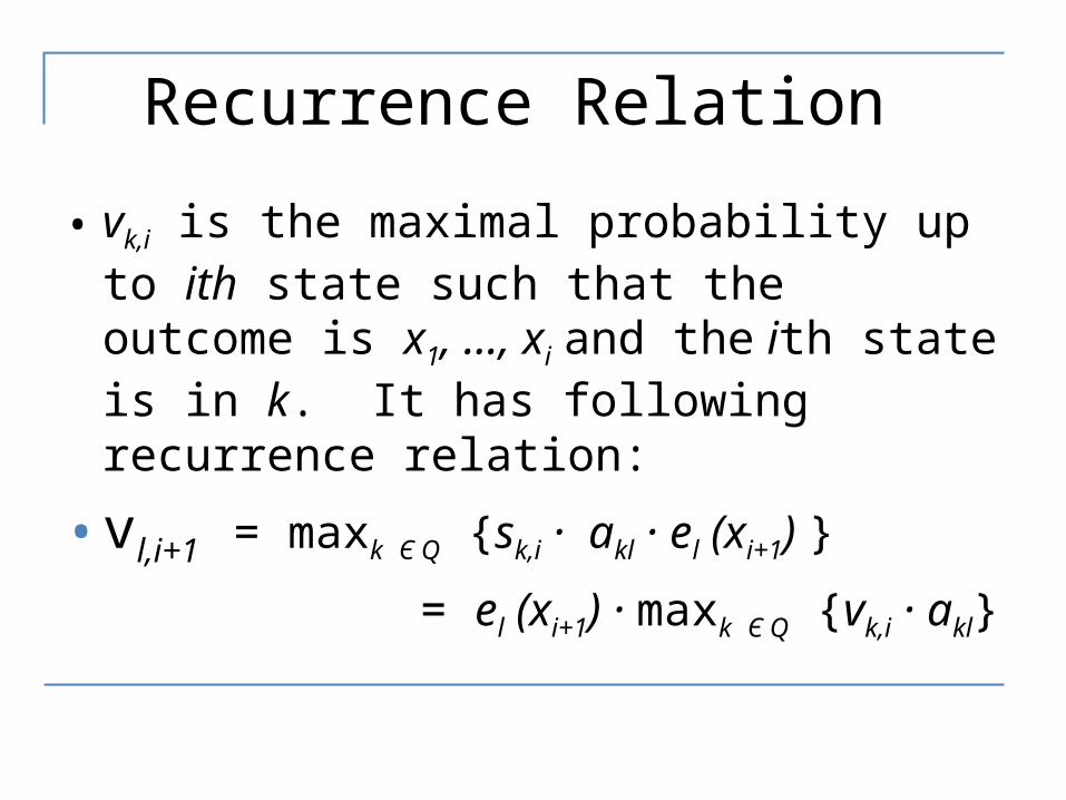
• vk,i is the maximal probability up to ith state such that the outcome is x1, …, xi and the ith state is in k. It has following recurrence relation:

• vl,i+1 = maxk Є Q {sk,i · akl · el (xi+1) }

= el (xi+1) · maxk Є Q {vk,i · akl}

Decoding Problem (cont’d)

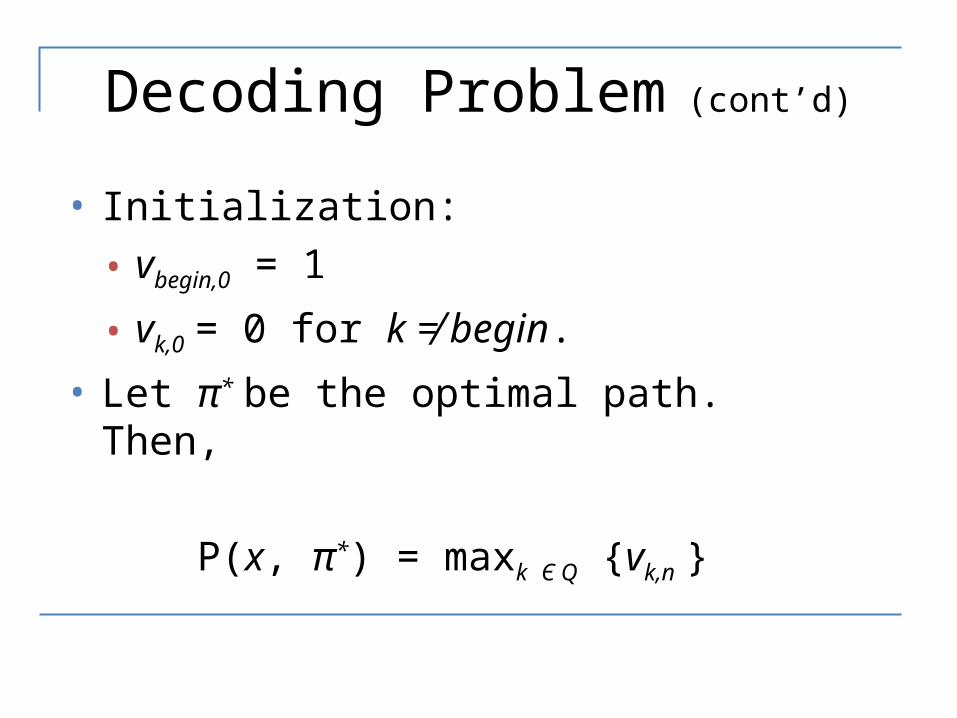
• Initialization:

• vbegin,0 = 1

• vk,0 = 0 for k ≠ begin.

• Let π* be the optimal path. Then,

P(x, π*) = maxk Є Q {vk,n }

Viterbi Algorithm

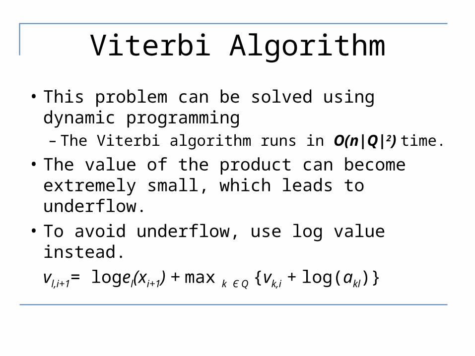
• This problem can be solved using dynamic programming– The Viterbi algorithm runs in O(n|Q|2) time.

• The value of the product can become extremely small, which leads to underflow.

• To avoid underflow, use log value instead. vl,i+1= logel(xi+1) + max k Є Q {vk,i + log(akl)}

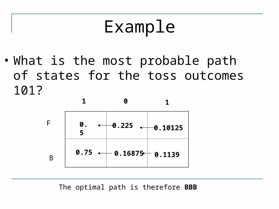
Example

• What is the most probable path of states for the toss outcomes 101?

1 0 1

F

B

The optimal path is therefore BBB

0.5

0.75

0.225

0.16875

0.10125

0.1139

Forward & Viterbi Algorithms

• Forward/Viterbi algorithms effectively consider all possible paths for a sequence– Forward to find probability of a sequence– Viterbi to find most probable path

39

POSTERIOIR PROBABILITY

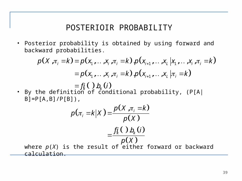
• Posterior probability is obtained by using forward and backward probabilities.

• By the definition of conditional probability, (P[A|B]=P[A,B]/P[B]),

where p(X) is the result of either forward or backward calculation.

1 1 1

1 1

, , , , . , , , , ,

, , , . , ,

.

i i i i L i i

i i i L i

k k

p X k p x x k p x x x x k

p x x k p x x k

f i b i

,

.

ii

k k

p X kp k X

p X

f i b i

p X

40

POSTERIOIR PROBABILITY

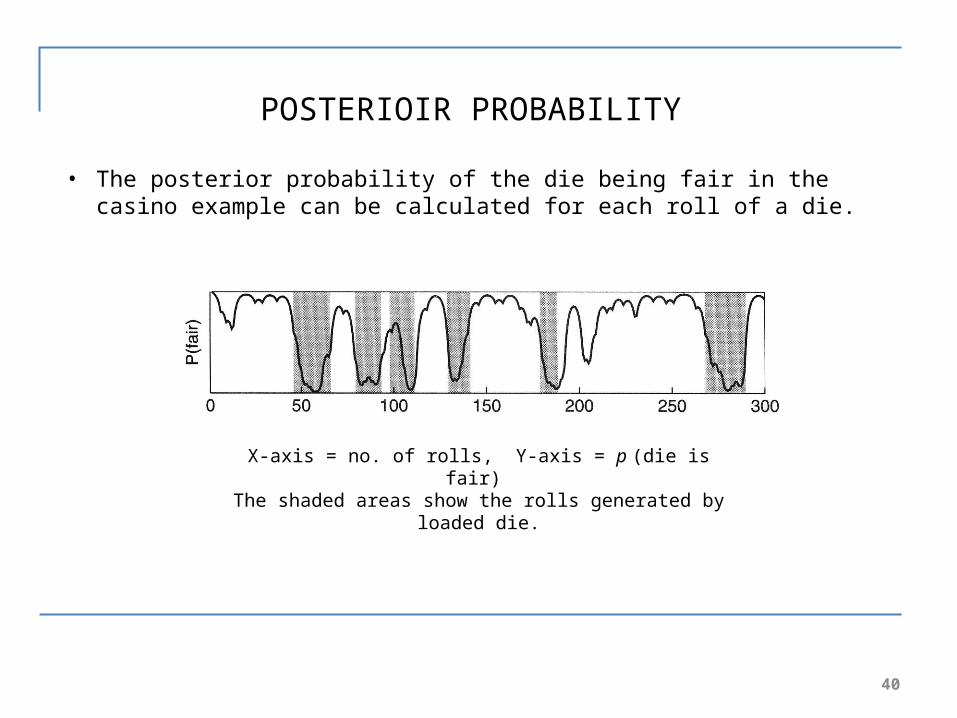
• The posterior probability of the die being fair in the casino example can be calculated for each roll of a die.

X-axis = no. of rolls, Y-axis = p (die is fair) The shaded areas show the rolls generated by

loaded die.

41

PARAMETER ESTIMATION FOR HMM

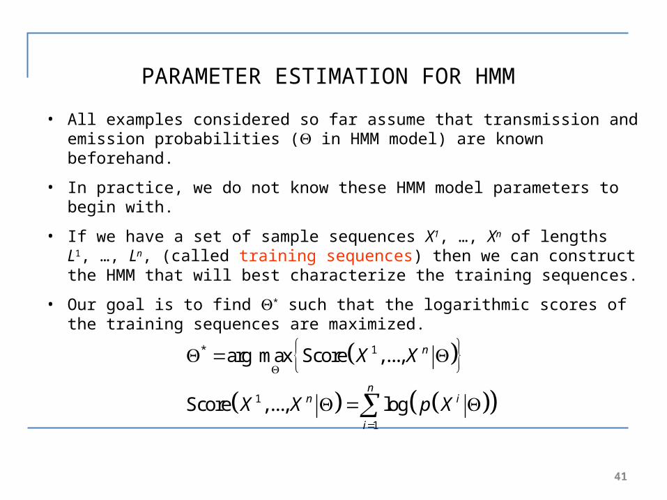
• All examples considered so far assume that transmission and emission probabilities ( in HMM model) are known beforehand.

• In practice, we do not know these HMM model parameters to begin with.

• If we have a set of sample sequences X1, …, Xn of lengths L1, …, Ln, (called training sequences) then we can construct the HMM that will best characterize the training sequences.

• Our goal is to find * such that the logarithmic scores of the training sequences are maximized.

* 1

1

1

arg max Score ,...,

Score ,..., log

n

nn i

i

X X

X X p X

42

ESTIMATION WHEN STATE SEQUENCE KNOWN

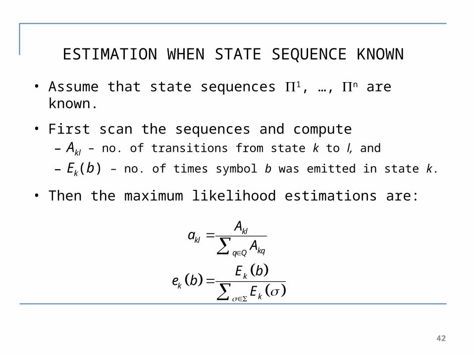
• Assume that state sequences 1, …, n are known.

• First scan the sequences and compute – Akl – no. of transitions from state k to l, and

– Ek(b) – no. of times symbol b was emitted in state k.

• Then the maximum likelihood estimations are:

klkl

kqq Q

kk

k

Aa

A

E be b

E

43

ESTIMATION WHEN STATE SEQUENCE UNKNOWN

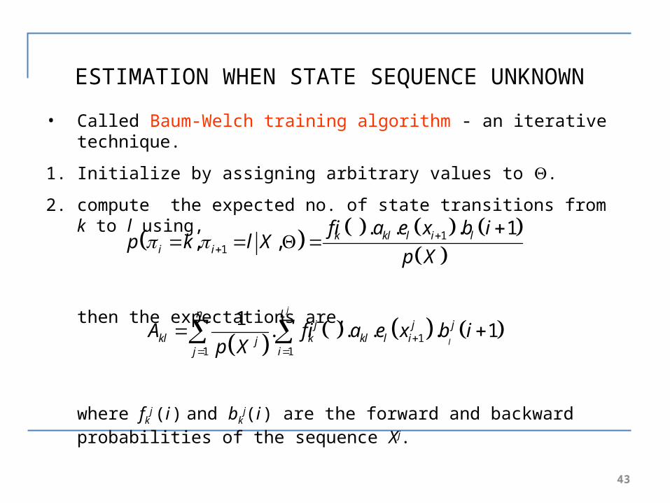
• Called Baum-Welch training algorithm - an iterative technique.

1. Initialize by assigning arbitrary values to .

2. compute the expected no. of state transitions from k to l using,

then the expectations are,

where fkj (i ) and bk

j(i ) are the forward and backward probabilities of the sequence Xj.

11

. . . 1, , k kl l i l

i i

f i a e x b ip k l X

p X

11 1

1. . . . 1

j

l

n Lj j j

kl k kl l ijj i

A f i a e x b ip X

44

ESTIMATION WHEN STATE SEQUENCE UNKNOWN…

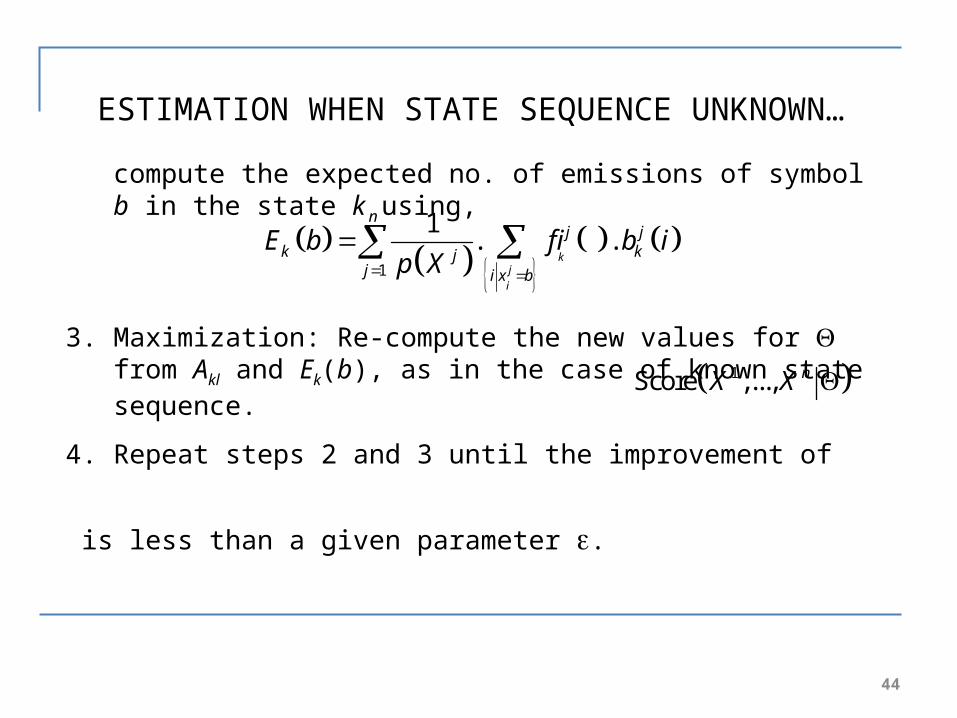
compute the expected no. of emissions of symbol b in the state k using,

3. Maximization: Re-compute the new values for from Akl and Ek(b), as in the case of known state sequence.

4. Repeat steps 2 and 3 until the improvement of

is less than a given parameter .

1

1. .

kj

i

nj j

k kjj i x b

E b f i b ip X

1Score ,..., nX X

Finding Distant Members of a Protein Family

• Motivation: Distant cousins of functionally related biological sequences in a protein family may have weak similarities to an individual sequence, and thus fail statistical tests, but may have similarities with many members of the family. So, the goal is to align a sequence to all members of the family at once.

• Family of related proteins can be represented by their multiple alignment and the corresponding profile.

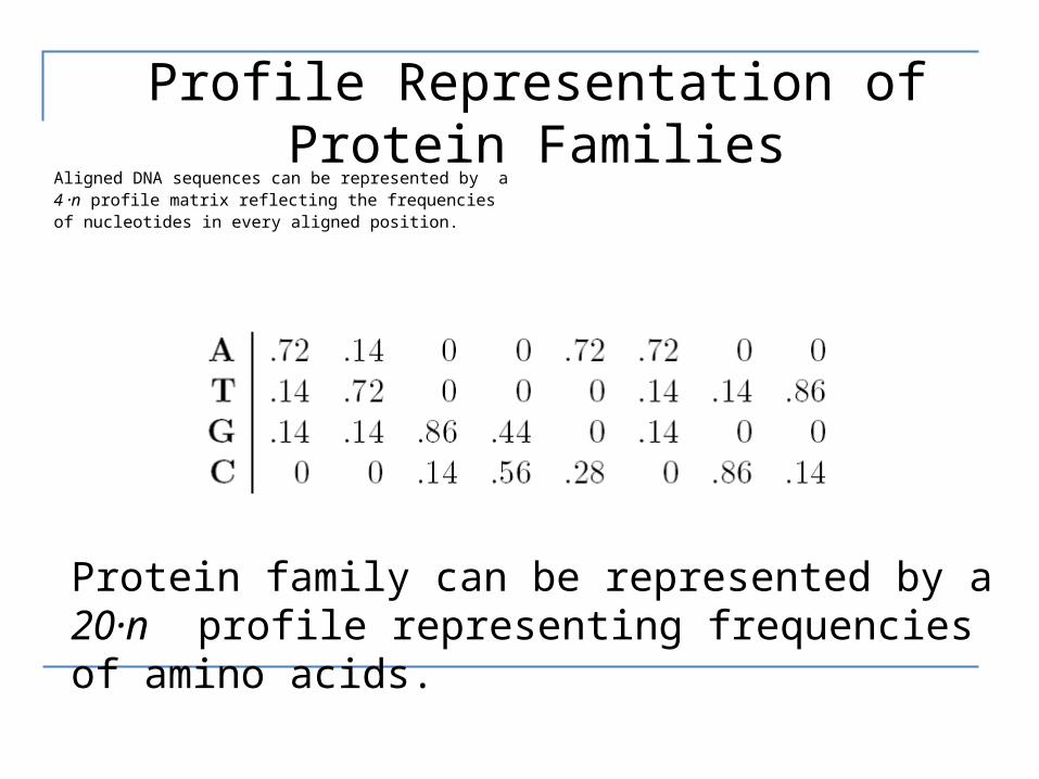
Profile Representation of Protein FamiliesAligned DNA sequences can be represented by a 4 ·n profile matrix reflecting the frequencies of nucleotides in every aligned position.

Protein family can be represented by a 20·n profile representing frequencies of amino acids.

Profile HMM

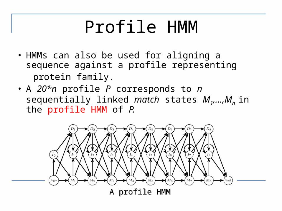
• HMMs can also be used for aligning a sequence against a profile representing

protein family.• A 20*n profile P corresponds to n sequentially linked

match states M1,…,Mn in the profile HMM of P.

A profile HMMA profile HMM

Insertion and Deletion States of Profile HMM

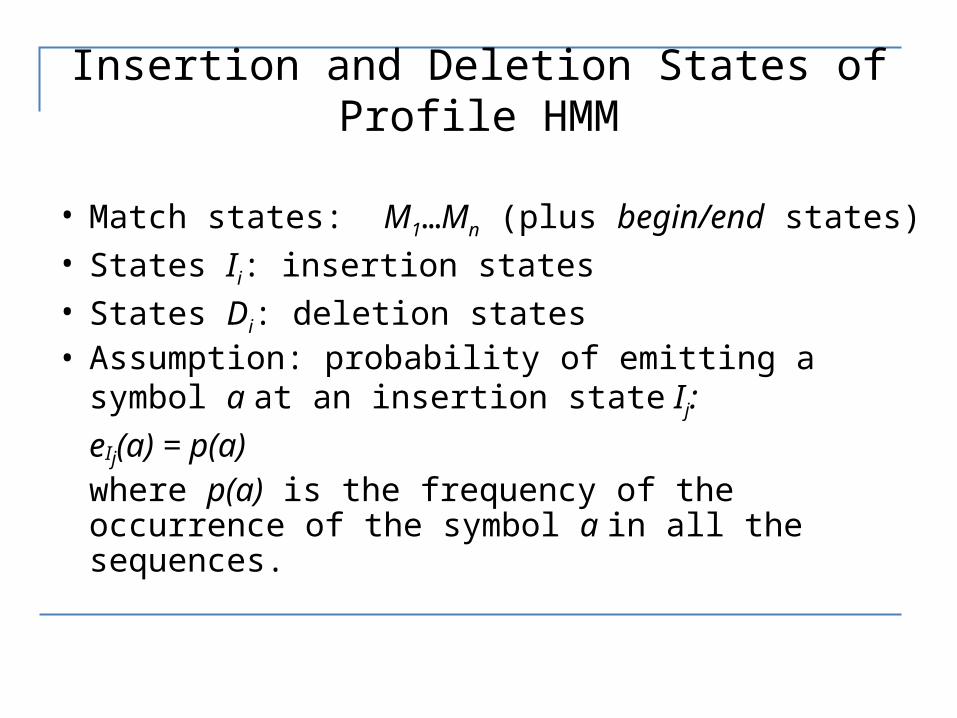
• Match states: M1…Mn (plus begin/end states) • States Ii: insertion states• States Di: deletion states• Assumption: probability of emitting a symbol a at an

insertion state Ij:eIj(a) = p(a)

where p(a) is the frequency of the occurrence of the symbol a in all the sequences.