Heuristic Route Search in Public Transportation Networks

BY

TIMOTHY MERRIFIELDB.S. in Computer Science, Ohio University, Athens, Ohio, 2004

THESIS

Submitted in partial fulfillment of the requirementsfor the degree of Master of Science in Computer Science

in the Graduate College of theUniversity of Illinois at Chicago, 2010

Chicago, Illinois

Copyright by

Timothy Merrifield

2010

This thesis is dedicated to my beautiful wife Amber and my parents Tim and Linda for their

relentless encouragement and support.

iii

ACKNOWLEDGMENT

This thesis is a joint effort with Dr. Jakob Eriksson of the BITS Networked Systems Lab-

oratory. Without his guidance, effort and infinite patience none of this work would have been

possible. I would also like to thank James Biagioni for guiding me through the TransitGe-

nie/Graphserver code base and helping me so much along the way.

TM

iv

TABLE OF CONTENTS

CHAPTER PAGE

1 INTRODUCTION . . . . . . . . . . . . . . . . . . . . . . . . . . . . . . . . . . 11.1 A Practical Motivation . . . . . . . . . . . . . . . . . . . . . . . . . 2

2 PRELIMINARIES AND RELATED WORK . . . . . . . . . . . . . . . 52.1 Graph Preliminaries and Definitions . . . . . . . . . . . . . . . . . 52.2 Classical Methods in Solving the Shortest Path Problem . . . . 62.3 Dijkstra’s Algorithm . . . . . . . . . . . . . . . . . . . . . . . . . . . 62.3.1 Bidirectional Dijkstra Search . . . . . . . . . . . . . . . . . . . . . 72.3.2 Best-First Search and Heuristic Functions . . . . . . . . . . . . . 72.3.3 The A* Algorithm and Admissible Heuristic Functions . . . . . 82.4 Definitions Related to Public Transportation Networks . . . . . 82.5 Contemporary Strategies . . . . . . . . . . . . . . . . . . . . . . . . 92.5.1 Arc Flags . . . . . . . . . . . . . . . . . . . . . . . . . . . . . . . . . . 92.5.2 Hierarchical Approaches . . . . . . . . . . . . . . . . . . . . . . . . 92.5.3 SHARC . . . . . . . . . . . . . . . . . . . . . . . . . . . . . . . . . . . 92.5.4 ALT . . . . . . . . . . . . . . . . . . . . . . . . . . . . . . . . . . . . . 92.5.5 Our Contribution . . . . . . . . . . . . . . . . . . . . . . . . . . . . . 10

3 A SEARCH HEURISTIC FOR PUBLIC TRANSPORTATIONNETWORKS . . . . . . . . . . . . . . . . . . . . . . . . . . . . . . . . . . . . . . 113.1 A* Search using Euclidean distance in multi-modal networks . 113.2 A Note on Bidirectional Dijkstra in Public Transportation Net-

works . . . . . . . . . . . . . . . . . . . . . . . . . . . . . . . . . . . . 123.3 Case Study: Dijkstra, Euclidean Distance and Our Heuristic . 123.4 A Heuristic for Public Transportation Systems . . . . . . . . . . 133.4.1 The Importance of Transitional Edges . . . . . . . . . . . . . . . 153.5 Grid Partitions . . . . . . . . . . . . . . . . . . . . . . . . . . . . . . 153.5.1 Uniform Grid Partitions . . . . . . . . . . . . . . . . . . . . . . . . . 153.5.2 Partitioning with Kd-Trees . . . . . . . . . . . . . . . . . . . . . . . 163.6 All Pairs Precomputation . . . . . . . . . . . . . . . . . . . . . . . . 163.6.1 Speeding up the Precomputation . . . . . . . . . . . . . . . . . . . 17

4 EVALUATION . . . . . . . . . . . . . . . . . . . . . . . . . . . . . . . . . . . . . 264.1 Methodology . . . . . . . . . . . . . . . . . . . . . . . . . . . . . . . . 264.2 Real-World Searches Extracted from the TransitGenie Logs . . 274.3 Searches within the City . . . . . . . . . . . . . . . . . . . . . . . . 284.4 Longer Searches Involving Suburban Areas . . . . . . . . . . . . 28

v

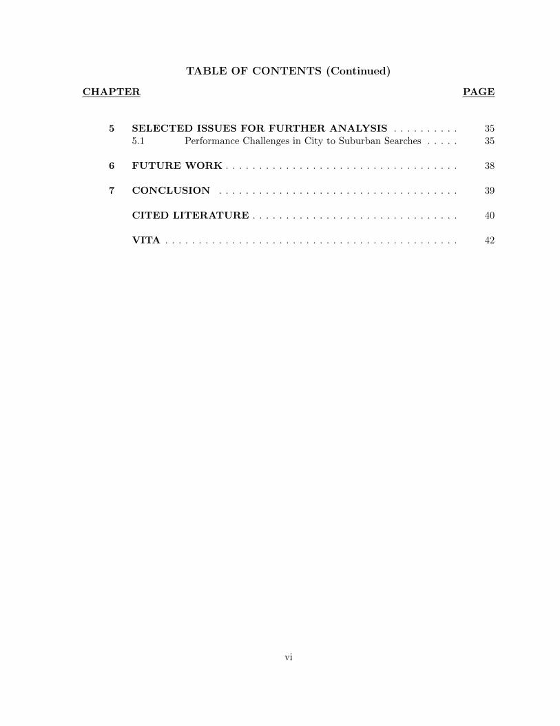
TABLE OF CONTENTS (Continued)

CHAPTER PAGE

5 SELECTED ISSUES FOR FURTHER ANALYSIS . . . . . . . . . . 355.1 Performance Challenges in City to Suburban Searches . . . . . 35

6 FUTURE WORK . . . . . . . . . . . . . . . . . . . . . . . . . . . . . . . . . . . 38

7 CONCLUSION . . . . . . . . . . . . . . . . . . . . . . . . . . . . . . . . . . . . 39

CITED LITERATURE . . . . . . . . . . . . . . . . . . . . . . . . . . . . . . . 40

VITA . . . . . . . . . . . . . . . . . . . . . . . . . . . . . . . . . . . . . . . . . . . . 42

vi

LIST OF TABLES

TABLE PAGE

I ABBREVIATIONS USED IN THE EVALUATION. . . . . . . . . . . 26

II AVERAGE PERFORMANCE IMPROVEMENT OVER DIJKSTRA 27

vii

LIST OF FIGURES

FIGURE PAGE

1 A single-source single-destination search using Dijkstra’s algorithm. . . 3

2 A CDF of the execution time of 5,000 queries taken from the Transit-Genie logs. . . . . . . . . . . . . . . . . . . . . . . . . . . . . . . . . . . . . . . . 4

3 The effects of inaccurate lower bounds on A* . . . . . . . . . . . . . . . . . 19

4 A search conducted using Dijkstra, A* with Euclidean distance heuristicand A* with our heuristic. . . . . . . . . . . . . . . . . . . . . . . . . . . . . . 20

5 A uniform grid partitioning the graph into 12 cells. . . . . . . . . . . . . . 21

6 The effects of inaccurate lower bounds on A* . . . . . . . . . . . . . . . . . 22

7 A 50x50 uniform grid partition. . . . . . . . . . . . . . . . . . . . . . . . . . 23

8 A simple kd-tree example and the cells it generates. . . . . . . . . . . . . 24

9 A kd-tree partition with approximately 8,000 cells. . . . . . . . . . . . . . 25

10 A CDF of the search space of several techniques tested against 5,000queries taken from the TransitGenie logs. . . . . . . . . . . . . . . . . . . . . 29

11 A CDF of the search space of our 5,000 queries using a log scale. . . . . 30

12 CDF of short searches within the downtown area of Chicago . . . . . . . 31

13 CDF of long searches within the city of Chicago . . . . . . . . . . . . . . . 32

14 CDF of searches from the downtown area of Chicago to suburban areas. 33

15 CDF of searches from suburban areas to the downtown area of Chicago. 34

16 A single city to suburbs query executed at various times over the courseof an hour. . . . . . . . . . . . . . . . . . . . . . . . . . . . . . . . . . . . . . . . 37

viii

CHAPTER 1

INTRODUCTION

Public transportation is a particularly attractive method of travel in urban areas. Travelers

choose public transportation for a variety of reasons including: reduced cost, environmental

concerns and convenience. However, despite the popularity of public transportation, only rel-

atively recently have researchers begun to develop algorithms to efficiently compute shortest

paths in this class of networks.

In recent years a tremendous amount of work has been done to speed up shortest path

computations on static road networks. However, not all of that work is applicable to public

transportation networks. This is due to the time dependency in a public transportation net-

work. The shortest path between a source and a destination in a public transportation network

can change depending upon the time at which the query is executed. We are also interested

in supporting real-time updates to the schedule (based on GPS data) which adds additional

complexity.

This thesis presents a precomputation-based heuristic that speeds up shortest path queries in

public transportation networks while preserving route optimality. Our heuristic is also schedule

independent and thus it is general enough to be used along with real-time data.

1

2

1.1 A Practical Motivation

Given an origin and a destination, TransitGenie (11) returns real-time, multi-modal public

transportation routes to the user. The modes currently supported are buses, trains and walking.

The searches are performed over the graph of the Chicagoland area which contains over 1.5

million vertices and over 4 million edges. The routing engine is derived from Graphserver (13)

and uses a simple Dijkstra search that terminates when the search expands the destination

vertex.

With this search strategy and a fairly large graph it is not surprising that many queries

will perform poorly. Figure 1 demonstrates a search from the Chicago downtown area to a

near-suburban area. Dijkstra’s algorithm visits over 200,000 vertices during the search and

takes 2.5 seconds to execute.

Figure 2 shows a CDF demonstrating this issue using 5,000 actual queries from the Transit-

Genie web logs (times shown are solely based on the search algorithm and exclude any HTTP

Request/Response overhead). The CDF shows that over 15% of the queries executed on the

system take over a second and 5% take over 2.5 seconds. To improve the performance and

scalability of the TransitGenie routing engine we began looking for algorithmic solutions to our

slow searches.

3

S

D

Figure 1. A single-source single-destination search using Dijkstra’s algorithm.

4

0

500

1000

1500

2000

2500

3000

0 0.1 0.2 0.3 0.4 0.5 0.6 0.7 0.8 0.9 1

Tim

e of

Exe

cutio

n (m

s)

Dijkstra

Figure 2. A CDF of the execution time of 5,000 queries taken from the TransitGenie logs.

CHAPTER 2

PRELIMINARIES AND RELATED WORK

We begin with some common definitions and classical methods followed by more recent work

in shortest path algorithms.

2.1 Graph Preliminaries and Definitions

A simple directed graph G is comprised of {V,E} s.t. V is a set of vertices and E is a set

of edges. Edges are binary relationships between vertices (u, v) such that u, v in V and u ≠ v.

A graph is also sometimes referred to as a network. A cost function c(e) associates positive

weights with all edges e ∈ E. Two vertices are adjacent if there exists some edge connecting

them.

A path between a source vertex v1 and a destination vertex vn in V is a sequence of adjacent

vertices {v1, v2, ..., vn−1, vn}. If a graph G is connected then ∀vi, vj in V there exists a path

between vi and vj. If a single path exists then there also exists an optimal shortest path with

respect to the cost function c. The shortest path problem is the problem associated with finding

the shortest path between two vertices.

An algorithm that solves the shortest path problem can be analyzed by observing its search

space. The search space can be defined as the number of vertices that must be explored from

s before the shortest path to d is discovered.

5

6

2.2 Classical Methods in Solving the Shortest Path Problem

The following section describes several classical methods in solving the shortest path problem

given a source vertex s and a destination vertex d. Further information can be found in

(2)(3)(4).

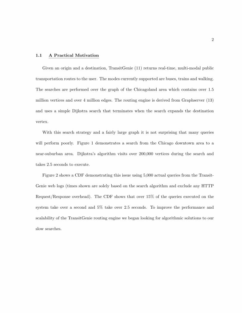
2.3 Dijkstra’s Algorithm

The canonical method for computing optimal shortest paths beginning from some source

vertex s ∈ V with non-negative edge weights is Dijkstra’s algorithm. The algorithm maintains

the following state ∀ u ∈ V: cost(u) which is the current best known cost (the total cost of best

known path) to u from s, settled(u) which is a boolean function for whether the lowest cost

path has been found to vertex u, and parent(u) which is the parent of u along the shortest

path. Initially, ∀ u ∈ V s.t. v ≠ s, cost(u) is set to ∞ and settled(u) is false. For s, cost(s)

is initialized to 0.

We start at s and set settled(s) to true and explore all of its adjacent vertices u1 to un. If

the cost from s to some vertex ui is less than cost(ui) then we update cost(ui) with the new

cost and set parent(ui) to vertex s. The next vertex to settle is chosen by finding the vertex

with the lowest known cost that has not yet been settled. The algorithm is terminated when

all vertices have been visited.

If the shortest path to only a single destination vertex d is desired then Dijkstras algorithm

can be modified to terminate when settled(d) is true. In chapter 5 this variation will be used

in comparison with our heuristic search.

7

Here it is important to note that similar to the previously discussed methods Dijkstra’s

algorithm will make no attempt to direct the search towards our destination vertex d. The

search space will expand outwards in all directions around the source vertex with no direction.

To minimize the search space we must look to other methods.

2.3.1 Bidirectional Dijkstra Search

One method of reducing the search space in the shortest path problem is to execute a

Dijkstra search from both s and d simultaneously. We can determine when the frontiers meet

by checking whether a vertex has been settled by both searches. If it has we have found the

shortest path and we can terminate the algorithm. This technique is optimal and can reduce

the size of the search space by as much as half.

2.3.2 Best-First Search and Heuristic Functions

Best-first search algorithms attempt to provide some direction to the search process and

subsequently reduce the search space. They are referred to as best-first because the best ver-

tices are chosen for exploration based on some function f(v). This class of algorithms is also

sometimes referred to as informed search strategies. A crucial component to this function f(v)

is a heuristic function h(v,d) which provides a lower bound on the cost of the route between

some vertex v and the destination d. A well known heuristic function is the Euclidean distance

between v and d.

A greedy best-first search is simply when f(v)=h(v,d). This means that we choose vertices

for exploration based solely on our heuristic function. This method can reduce the search space

dramatically but is not guaranteed to find the optimal path.(3)

8

2.3.3 The A* Algorithm and Admissible Heuristic Functions

The A* algorithm provides a nice compromise between the reduced search space of greedy-

best-first search and the optimality of Dijkstra’s search. It essentially performs Dijkstra’s

search but it chooses vertices for expansion based on the function f(v) = cost(v) + h(v,d). A*

is guaranteed to find optimal solutions if the heuristic function is admissible. An admissible

heuristic function never overestimates the cost to the destination vertex. An extreme example

would be for h(v,d)=0 for all v. In this case A* would perform exactly like Dijkstra’s algorithm.

However, if h(v,d) can provide accurate lower bounds to d then A* can reduce the search space

while still providing optimal paths.(4)(3)

2.4 Definitions Related to Public Transportation Networks

A time-dependent graph G ′ utilizes a cost function cost(e, t) where t is the current time.

Therefore, the cost of taking an edge varies depending on the time at which the query is

executed. A time-dependent graph can also be referred to as a dynamic graph. A public

transportation network is a time-dependent graph due to the schedules for buses and trains.

Also, because there are varying modes of transportation in these networks we can describe

them as multi-modal networks. The alternative would be a single mode network such as a road

network where the only mode of transportation is a car.

The time-dependency and multi-modal nature of these networks adds additional complexity

to the shortest path problem. In Chapter 3 we will discuss how this complexity impacts some

of the techniques described in this chapter.

9

2.5 Contemporary Strategies

2.5.1 Arc Flags

Arc flags (6)(7) is a technique where we keep track of whether or not an arc is on the shortest

path to a destination. Since storing a flag at every edge for every vertex is not possible for large

graphs, the graph is instead partitioned into regions. If an edge is on the shortest path to any

vertex in that region then we set the flag to true. Because arc weights are dynamic in public

transportation networks it would be difficult to apply this approach. However, the heuristic

presented in this thesis makes use of many techniques used in arc flags.

2.5.2 Hierarchical Approaches

In (9) the intuition of routing in road networks is reduced to local search and highway

search. A local search explores edges at the end points (source and destination) of the search

while highway edges connect the local searches. The precomputation algorithm can be applied

recursively forming multi-level contracted graphs. Contraction Hierarchies (10) further expand

the notion of contraction with a more sophisticated contraction technique.

2.5.3 SHARC

SHARC (8) combines hierarchical approaches and arc-flags into a unidirectional algorithm

that can support time dependency. It was shown to improve upon Dijkstra in schedule based

rail networks by approximately 100 times.

2.5.4 ALT

ALT (5) is a heuristic search that uses a set of landmarks to provide direction to the search.

The distance to and from the landmarks are precomputed for all vertices in the graph. The

10

technique works in such a way that if a segment is shared on the shortest path to the landmark

and the destination, then it will be explored first. This works well in a road network where

normally a shortest path will involve a few local edges, then a highway and then more local

edges. In a road network a landmark can be very far away from the destination and yet share

many edges along the shortest path (the first set of local edges and a portion of the highway

for instance).

2.5.5 Our Contribution

Many of the techniques described above are designed for static road networks. Those that

can be applied to public transportation networks perform contraction or precomputation that

is based on schedules. Our contribution is a partitioning based heuristic that is schedule inde-

pendent and works in dynamic networks.

CHAPTER 3

A SEARCH HEURISTIC FOR PUBLIC TRANSPORTATION

NETWORKS

We begin this chapter by describing some of the difficulties associated with finding shortest

paths in a public transportation network. We then present a novel heuristic that works in this

class of networks.

3.1 A* Search using Euclidean distance in multi-modal networks

As discussed earlier, an informed search technique (such as A*) can direct the search towards

the destination using a heuristic function that approximates lower bounds. In order to satisfy

the criteria of an admissible heuristic, a function h(v,d) must never overestimate the cost to

the destination vertex.

In a multi-modal network we may have several possibilities for transport including walking,

bus, subway and high-speed trains. If our heuristic function is the Euclidean distance between

a given vertex and the destination, then the speed with which we travel along that straight-

line distance must be the velocity of our fastest mode of transportation. For the Chicago

transit graph, the heuristic then must use the speed of an express train. However, a large

portion of routes will not include this mode of transportation; therefore the heuristic provides

an inaccurate lower bound on the distance to the destination.

11

12

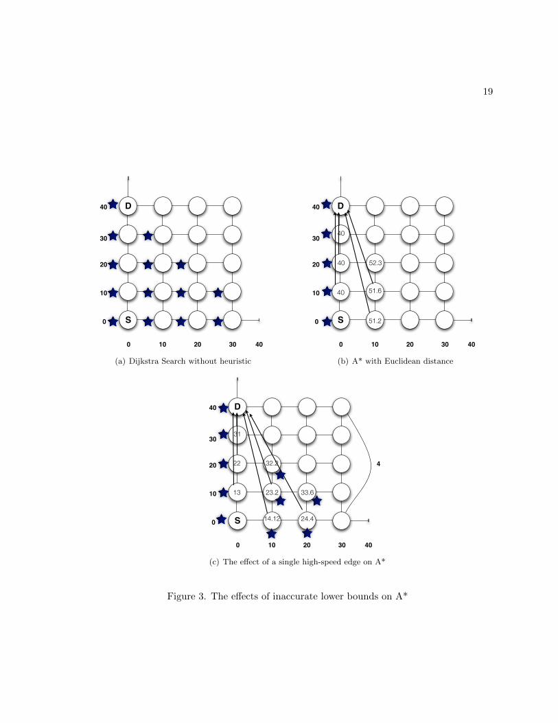
In Figure 3 we see an example of the issue in a simplistic graph topology. The explored

search space is shown by stars next to the vertices. Figure Figure 3(a) shows a simple Dijkstra

search while Figure Figure 3(b) illustrates the reduced search space using A* with a Euclidean

distance heuristic. However, when we add a single high-speed edge in Figure 3(c) we see that

the search space is once again increased by the loose lower bounds generated by the Euclidean

distance heuristic. As our lower-bounds become less accurate the number of vertices in our

search space begins to approach Dijkstra.

3.2 A Note on Bidirectional Dijkstra in Public Transportation Networks

A traditional bidirectional search begins at the destination vertex d and the source vertex

s at the same time and meets somewhere in the middle. However, in a public transportation

network we cannot execute a search starting at d because we do not know at what time to

begin (a necessary parameter when searching a transit network). We will not know that time

until we have executed a forward search and determined at which time we will arrive at d. Only

then can we begin executing the search in the backward direction. This makes a bidirectional

Dijkstra search very difficult to implement unless we permit estimation of the arrival time which

removes optimality. This is unfortunate because many nice techniques have been developed

using bidirectional search.

3.3 Case Study: Dijkstra, Euclidean Distance and Our Heuristic

Here we look at how our heuristic compares to Dijkstra’s algorithm and the Euclidean

distance heuristic for a single search within the Chicago public transportation graph. A de-

13

scription of our heuristic can be found in the next section and a more detailed evaluation of

these techniques will be discussed in Chapter 4.

Figure 4 shows three maps which detail the search space for a single query from downtown

Chicago to a suburb. It was noted earlier in this chapter that A* with a Euclidean distance

heuristic performs poorly in multi-modal networks. In 4(a) and 4(b) we see that the search space

(the dark region) is nearly identical for the two techniques. Dijkstra’s search space consists of

46,307 vertices while the Euclidean distance heuristic explores 19,516 vertices for this search.

While it is an improvement, it is not a dramatic one. Contrast this with the results of 4(c)

using our heuristic. The search space here is 800 vertices which yields approximately a 57x

improvement over Dijkstra and approximately a 24x improvement over the Euclidean distance

heuristic.

3.4 A Heuristic for Public Transportation Systems

It is well known that the best possible heuristic from some vertex v to a destination vertex

d would be the cost of the actual shortest path from v to d. If this information was known,

then a best-first search algorithm (such as Dijkstra’s) would only expand nodes on the shortest

path to the destination. Unfortunately, storing and computing this data for all-pairs is O(n2)

and is therefore out of the question for any graph with a large number of vertices. Also, the

dynamic nature of a public transportation network adds additional complexity because the cost

of the shortest path from v to d can vary based on the departure time from v.

We can reduce the storage and computational complexity of all-pairs by partitioning our

graph into a set of n cells, {c0...cn}. The most obvious way of performing the partitioning

14

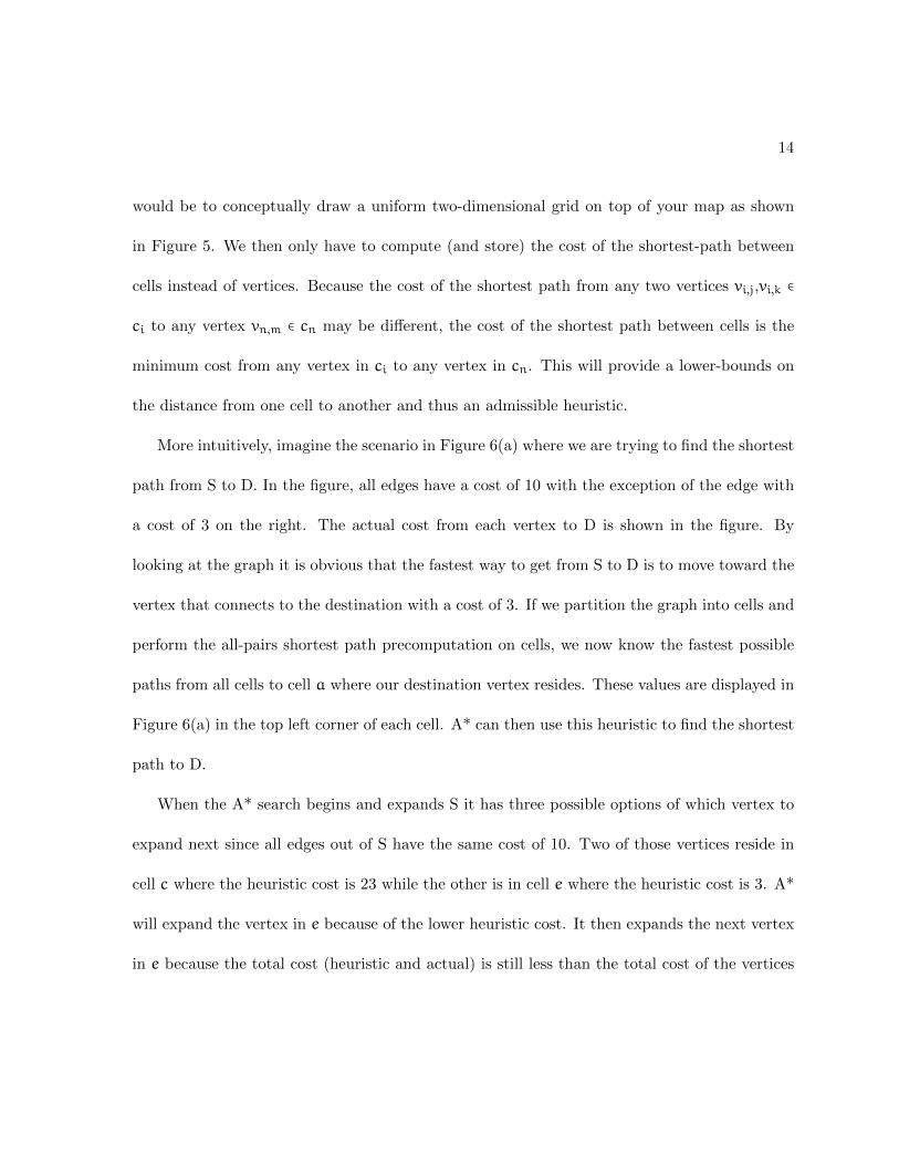
would be to conceptually draw a uniform two-dimensional grid on top of your map as shown

in Figure 5. We then only have to compute (and store) the cost of the shortest-path between

cells instead of vertices. Because the cost of the shortest path from any two vertices vi,j,vi,k ∈

ci to any vertex vn,m ∈ cn may be different, the cost of the shortest path between cells is the

minimum cost from any vertex in ci to any vertex in cn. This will provide a lower-bounds on

the distance from one cell to another and thus an admissible heuristic.

More intuitively, imagine the scenario in Figure 6(a) where we are trying to find the shortest

path from S to D. In the figure, all edges have a cost of 10 with the exception of the edge with

a cost of 3 on the right. The actual cost from each vertex to D is shown in the figure. By

looking at the graph it is obvious that the fastest way to get from S to D is to move toward the

vertex that connects to the destination with a cost of 3. If we partition the graph into cells and

perform the all-pairs shortest path precomputation on cells, we now know the fastest possible

paths from all cells to cell a where our destination vertex resides. These values are displayed in

Figure 6(a) in the top left corner of each cell. A* can then use this heuristic to find the shortest

path to D.

When the A* search begins and expands S it has three possible options of which vertex to

expand next since all edges out of S have the same cost of 10. Two of those vertices reside in

cell c where the heuristic cost is 23 while the other is in cell e where the heuristic cost is 3. A*

will expand the vertex in e because of the lower heuristic cost. It then expands the next vertex

in e because the total cost (heuristic and actual) is still less than the total cost of the vertices

15

in c. Intuitively, the heuristic is a hint to A* that a fast way to our destination can be found

in cell e.

3.4.1 The Importance of Transitional Edges

As we saw in the previous section, the heuristic value applies to all the vertices in a given

cell. Another way to say that is that given any vi, vj in cell ck and a destination vertex d,

h(vi, d)=h(vj, d). For this reason, our heuristic does not help us unless we are considering

vertices that are not in the same cell. Therefore, it is important to create a partition that

maximizes the total number of cells and the total number of transitional edges. A transitional

edge can be defined as an edge connecting two adjacent vertices that reside in different cells.

3.5 Grid Partitions

The following section describes the strategies used in creating the grid partitions. As we

will see later, the choice of a grid partition is critical to the performance of the heuristic.

3.5.1 Uniform Grid Partitions

The most simplistic way of partitioning the map is using a uniform 2-dimensional grid. We

define the resolution of the grid to be a value n s.t. the grid has n rows and n columns and

n∗n total cells. As discussed earlier, the heuristic is only taken into account when encountering

a transitional edge. Thus, a higher resolution grid will provide a larger number of transitional

edges. Of course, this is a trade-off between storage/precomputation time and performance. A

higher resolution grid will take longer to precompute and store but will yield better performance.

In Chapter 4 we will experiment with partitions of resolution 50 and 100.

16

3.5.2 Partitioning with Kd-Trees

A kd-tree(1) is a simple binary tree data structure designed to store multi-dimensional

spatial data. The ’k’ in the name denotes the structures ability to handle an arbitrary number

of dimensions. The partitioning algorithm works by alternating between dimensions and in our

case the tree will be 2d with our dimensions being latitude and longitude. It works recursively

by finding the median of a set of vertices in one dimension and then partitioning the cell into

two new cells based on that median. The two new cells are then split again by the same method,

except this time the other dimension is used. The recursion stops when the number of vertices

in a cell drops below a configurable threshold. Figure 8 shows a simple example of how a kd-tree

would partition a small number of points in 2-d Euclidean space. In our experiments we will

use a kd-tree with approximately 8,000 cells (150 vertex per cell threshold).

The kd-tree provides a nice partition based on the density of vertices in the graph. Intu-

itively, the graph will be partitioned such that the area with a high vertex density will be very

high resolution (small cell size) and the areas with a low vertex density will have low resolution

(large cell size). Figure 9 demonstrates the partition executed on the Chicago graph. Not

surprisingly, the area around downtown has a much higher resolution.

3.6 All Pairs Precomputation

The result of the precomputation step is that we determine the shortest path from all cells

to all other cells. Here min cost(ci, cj) is the minimum cost from any vertex in ci to any vertex

in cj. The simplest way to compute this is to run Dijkstra’s algorithm starting at each vertex in

the graph. If we begin from some source vertex in ci, any time that the search expands a vertex

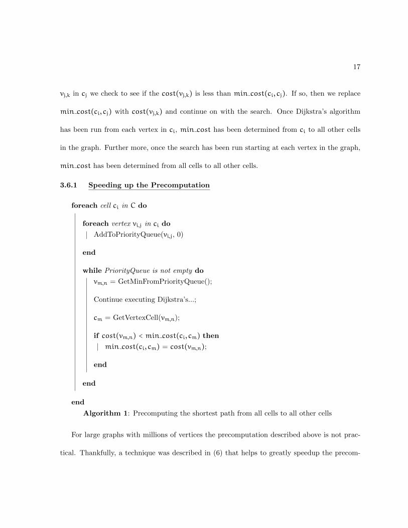
17

vj,k in cj we check to see if the cost(vj,k) is less than min cost(ci, cj). If so, then we replace

min cost(ci, cj) with cost(vj,k) and continue on with the search. Once Dijkstra’s algorithm

has been run from each vertex in ci, min cost has been determined from ci to all other cells

in the graph. Further more, once the search has been run starting at each vertex in the graph,

min cost has been determined from all cells to all other cells.

3.6.1 Speeding up the Precomputation

foreach cell ci in C do

foreach vertex vi,j in ci do

AddToPriorityQueue(vi,j, 0)

end

while PriorityQueue is not empty do

vm,n = GetMinFromPriorityQueue();

Continue executing Dijkstra’s...;

cm = GetVertexCell(vm,n);

if cost(vm,n) < min cost(ci, cm) then

min cost(ci, cm) = cost(vm,n);

end

end

end

Algorithm 1: Precomputing the shortest path from all cells to all other cells

For large graphs with millions of vertices the precomputation described above is not prac-

tical. Thankfully, a technique was described in (6) that helps to greatly speedup the precom-

18

putation step. Instead of running Dijkstra’s algorithm from each vertex in the graph we only

have to run the algorithm once per cell. If we are computing min cost for ci then we begin

the Dijkstra’s search by placing all vertices in ci into the priority queue with a cost of 0. This

effectively starts the search from every vertex in ci. This simple technique improves the run

time of the precomputation from O(∣V ∣) to O(∣C∣) where ∣C∣ is the number of cells in the graph.

The full algorithm is presented in Algorithm 1.

19

0 10 20 30

0

10

20

30

40

40

D

S

(a) Dijkstra Search without heuristic

0 10 20 30

0

10

20

30

40

40

D

S 51.2

40 51.6

40

40

52.3

(b) A* with Euclidean distance

0 10 20 30

0

10

20

30

40

40

4

D

S 14.12

13 23.2

22

24.4

32.2

31

33.6

(c) The effect of a single high-speed edge on A*

Figure 3. The effects of inaccurate lower bounds on A*

20

(a) Djikstra Search (b) A* with Euclidean distance heuristic

(c) A* with our heuristic

Figure 4. A search conducted using Dijkstra, A* with Euclidean distance heuristic and A*with our heuristic.

21

Figure 5. A uniform grid partitioning the graph into 12 cells.

22

(a) A graph with a high-speed linesimilar to a train in public trans-portation networks

323

33

10

0

a

b

c e

d

S

D

(b) Grid drawn over graphwhere the letter and number ineach cell are the cell identifierand the shortest path to cell a

respectively

Figure 6. The effects of inaccurate lower bounds on A*

23

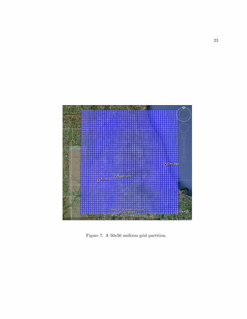
Figure 7. A 50x50 uniform grid partition.

24

1 2

1

2

3 4

4

3

5

5

6 7 8 9 10

6

7

8

9

10

Figure 8. A simple kd-tree example and the cells it generates.

25

Figure 9. A kd-tree partition with approximately 8,000 cells.

CHAPTER 4

EVALUATION

In this chapter we will describe the evaluation methodology used and the results of that

evaluation. Several types of queries are tested including both real-world queries (pulled from

the TransitGenie query logs) and synthetic queries subdivided into several different types.

4.1 Methodology

We evaluate all the grid types described above and compare them with Dijkstra’s and A*

with a Euclidean distance heuristic. Below is a table describing the abbreviations used in the

figures.

To evaluate the system we start with real world queries extracted from the TransitGenie

logs. We use the same 5,000 real world searches that were used in Chapter 1 to evaluate the

performance of different approaches. To get a more detailed view of the results we also use

TABLE I

ABBREVIATIONS USED IN THE EVALUATION.

Dijkstra’s algorithm (terminated at destination) D

A* with Euclidean distance ED

A* with 50x50 grid G50

A* with 100x100 grid G100

A* with kdtree KD

26

27

TABLE II

AVERAGE PERFORMANCE IMPROVEMENT OVER DIJKSTRA

Method Real Searches Short City Long City City to Suburbs Suburbs to City

ED 1.41x 1.29x 1.43x 1.17x 1.44x

G50 2.42x 1.49x 3.89x 1.53x 2.57x

G100 3.47x 2.22x 5.90x 1.83x 3.19x

KD 6.09x 5.15x 10.56x 1.57x 3.40x

synthetic queries we generate ourselves that fall into several different types of searches. The

synthetic queries are broken up into the following classes: short searches within the city, long

searches within the city, searches from the city to the suburbs, and from the suburbs to the

city.

4.2 Real-World Searches Extracted from the TransitGenie Logs

Using the same set of queries shown in Chapter 1 we evaluate the different techniques. As

we can see in Figure 10 the success of the techniques is dependent on the number of transitional

edges that factor into the problem space. For this reason the kd-tree’s higher resolution does

very well with this problem set. Also as expected, the 100x100 grid is consistently better than

the 50x50 grid. The Euclidean distance heuristic provides marginal gains over the Dijkstra

search.

While there is improvement (the kd-tree does over 6 times better than Dijkstra on average),

there are still searches that do very poorly. This can be seen in the 85’th percentile of the log

28

scale plot in Figure 11. To better understand these performance numbers we generated our

own synthetic queries for a more in depth analysis.

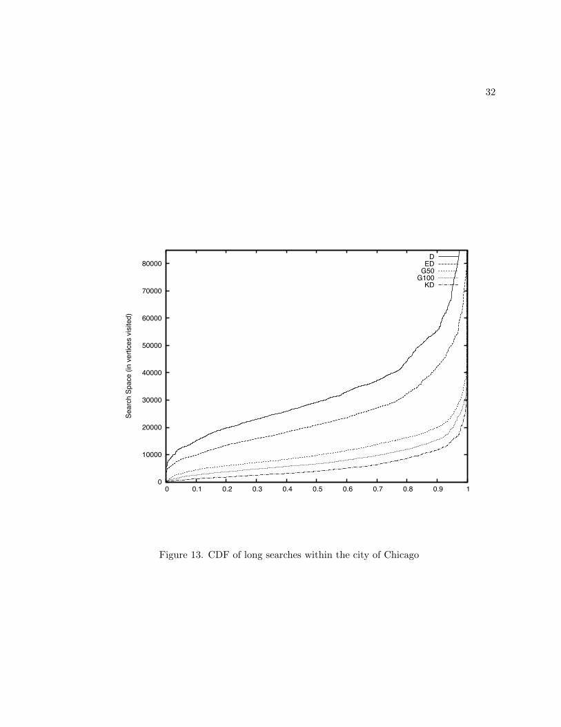
4.3 Searches within the City

We tested both searches that covered large portions of the city and searches that covered a

relatively short distances (just several blocks in some cases). CDF plots of these two data sets

can be found in Figure 12 and Figure 13. Looking at Table II we can see that a kd-tree partition

does very well for queries within the city, resulting with an average 10x performance improve-

ment over Dijkstra for longer city queries. The 100x100 grid shows a non-trivial improvement

over the Dijkstra search as well.

4.4 Longer Searches Involving Suburban Areas

We also performed searches covering a larger portion of the Chicagoland area including

suburban regions. These searches tend to utilize the higher speed commuter rail lines that

operate between the city and the suburbs. Examining the numbers in Table II we can see that

the speedup from the city to the suburbs is disappointing for all techniques. CDF’s for both

city to suburbs and suburbs to city searches are found in Figure 14 and Figure 15. Both the

kd-tree and grid partitions struggle to even improve the Dijkstra search by 2x. We speculate

that the 100x100 grid does the best because it has a more constant resolution over the entire

graph. In Chapter 5 we will discuss in detail why the speedup is so moderate on these longer

searches.

29

0

5000

10000

15000

20000

25000

30000

35000

40000

0 0.2 0.4 0.6 0.8 1

Sear

ch S

pace

(in

verti

ces

visite

d)

DED

G50G100

KD

Figure 10. A CDF of the search space of several techniques tested against 5,000 queries takenfrom the TransitGenie logs.

30

10

100

1000

10000

100000

1e+06

1e+07

0 0.2 0.4 0.6 0.8 1

Sear

ch S

pace

(in

verti

ces

visite

d)

DED

G50G100

KD

Figure 11. A CDF of the search space of our 5,000 queries using a log scale.

31

0

2000

4000

6000

8000

10000

12000

14000

0 0.1 0.2 0.3 0.4 0.5 0.6 0.7 0.8 0.9 1

Sear

ch S

pace

(in

verti

ces

visite

d)

DED

G50G100

KD

Figure 12. CDF of short searches within the downtown area of Chicago

32

0

10000

20000

30000

40000

50000

60000

70000

80000

0 0.1 0.2 0.3 0.4 0.5 0.6 0.7 0.8 0.9 1

Sear

ch S

pace

(in

verti

ces

visite

d)

DED

G50G100

KD

Figure 13. CDF of long searches within the city of Chicago

33

0

100000

200000

300000

400000

500000

600000

700000

800000

900000

0 0.1 0.2 0.3 0.4 0.5 0.6 0.7 0.8 0.9 1

Sear

ch S

pace

(in

verti

ces

visite

d)

DED

G50G100

KD

Figure 14. CDF of searches from the downtown area of Chicago to suburban areas.

34

0

10000

20000

30000

40000

50000

60000

70000

80000

90000

100000

0 0.1 0.2 0.3 0.4 0.5 0.6 0.7 0.8 0.9 1

Sear

ch S

pace

(in

verti

ces

visite

d)

DED

G50G100

KD

Figure 15. CDF of searches from suburban areas to the downtown area of Chicago.

CHAPTER 5

SELECTED ISSUES FOR FURTHER ANALYSIS

In the previous chapter we discussed the implementation, the evaluation methodology and

the results of the evaluation. However, several of the results were non-intuitive. In this chapter

we will attempt to shed some light on some of those issues.

5.1 Performance Challenges in City to Suburban Searches

In the previous chapter we saw that the city to suburban searches tended to still yield very

high search spaces for all of our heuristic techniques. The reason for this is simple, these routes

tend to use the higher speed commuter rail system that has relatively infrequent departure times

when compared to other modes of transit. For instance, a common pattern is for a train to

leave from a given station once every hour. When we perform our precomputation the shortest

path from a city cell to a suburban cell will almost certainly use this mode of transit. However,

the precomputation ignores all delay and provides us with the fastest possible route between

cells. Intuitively, this means that the heuristic value is based on the notion that the train is

sitting there waiting for you to arrive and then immediately departs.

When a search query is executed the heuristic directs the search towards the train station.

However, in the worst case condition we have just missed the train and have to wait as much as

55 minutes for the next train. Of course, our algorithm does not spend this 55 minutes waiting

around. It will continue to search for faster routes during this time. Figure 16 demonstrates

35

36

this phenomenon. Here a single query between the city and the suburbs is executed several

times over the course of an hour. For the kd-tree, in the best case it improves over Dijkstra by

2.25x and in the worst case 1.25x. The best case occurs when the search arrives at the train

station just in time to catch the train and the worst case occurs when we just missed the train.

This issue was described in (12) as a problem of bad connectivity and is major problem

with all heuristic searches in public transportation networks. When there is higher connectivity

our heuristic can make some improvements however in this worst case it begins to approach

Dijkstra.

37

40000

60000

80000

100000

120000

140000

160000

180000

200000

220000

0 10 20 30 40 50 60

Searc

h S

pace (

in v

ert

ices v

isited)

KDD

Minutes from the top of the hour

1.27x

2.25x

Figure 16. A single city to suburbs query executed at various times over the course of an hour.

CHAPTER 6

FUTURE WORK

We have shown that a simple precomputed heuristic can speed up certain classes of searches

several times over Dijkstra. While this is a significant improvement, it is troubling that the issue

of disconnectivity causes our optimization to perform sub-optimally on the class of searches (city

to suburbs) that result in the highest query times. So the issue becomes, how can we improve

our scheme to handle disconnectivity?

To solve the issue we plan to add an additional dimension to our heuristic, time. In Chapter

5 we discussed how the start time of our search is critical to minimizing the search space,

particularly for searches that are relatively disconnected. This is because our heuristic was

precomputed ignoring delay and storing the lowest possible cost (over all times) to a destination

cell. If we create a partition with an additional time range property, we could compute the

lowest cost for just that time range. We expect precomputation values based on certain ranges

to produce more accurate lower bounds and reduce the search space.

It my appear that adding the time range property would cause the cell count to grow

tremendously but it may not be so bad. Imagine a high-speed commuter rail line with trains

leaving every hour. Each hour interval can be divided into 15 minute intervals and the common

intervals can be attached to the same cell. For example, the following intervals: 12:00-12:15,

1:00-1:15, 2:00-2:15 could be associated with one cell because they should have very similar

lower bounds.

38

CHAPTER 7

CONCLUSION

We have shown that given a suitable heuristic and a moderate amount of precomputation,

we can see a tremendous speedup for certain classes of queries while maintaining optimality.

Performing experiments on the Chicagoland graph, our heurisitic does 6x better on average

than Dijkstra and 10x better on certain classes of queries. In the future, we look forward

to continuing to improve the performance particularly on queries that involve a high level of

disconnectivity.

39

CITED LITERATURE

1. JL Bentley: Multidimensional Binary Search Trees Used for Associative Searching Comm.ACM, pages 509–517, 1975.

2. RE Korf: Depth-First Iterative Deepening: An Optimal Admissable Tree Search ArtificialIntelligence 27 (1), Pages 97-109, 1985 .

3. SJ Russell, P Norvig: Artificial Intelligence: A Modern Approach Englewood Cliffs, NJ:Prentice Hall, 1995

4. PE Hart, NJ Nilsson, and B Raphael: A Formal Basis for the Heuristic Determination ofMinimum Cost Paths. IEEE Transactions on System Science and Cybernetics 4(2)1968.

5. AV Goldberg, C Harrelson Computing the shortest path: A* search meets graph theory InProc. 16th ACM-SIAM Symposium on Discrete Algorithms Pages 156-165 2005.

6. M Hilger, E Kohler, R Mohring, and H Schilling.: Fast Point-to-Point Shortest PathComputations with Arc-Flags. MobiSys, 2008.

7. R Mohring, H Schilling, B Schutz, D Wagner and T Willhalm. Partitioning Graphs toSpeedup Dijkstras Algorithm. ACM Journal of Experimental Algorithmics11(2),2006.

8. R Bauer, D Delling SHARC: Fast and robust unidirectional routing ACM Journal ofExperimental Algorithmics14(2), 2009.

9. P. Sanders and D. Schultes Fast and Exact Shortest Path Queries Using Highway Hierar-chies. Proc. 13th Annual European Symposium Algorithms, 2005.

10. R. Geisberger Contraction hierarchies: Faster and simpler hierarchical routing in roadnetworks, 2008. Diploma Thesis, Universitat Karlsruhe.

11. J. Biagioni, A. Agresta, T. Gerlich, and J. Eriksson.

Transitgenie: A real-time, context-aware transit navigator (demo abstract). SenSys,ACM, 2009 pages 329-330.

40

41

12. H Best. Car or Public Transport–Two Worlds Lecture Notes In Computer Science(5760),2009.

13. Graphserver, the open-source multi-modal trip planner. http://graphserver.github.

com/graphserver/.

VITA

Timothy Merrifield

.

Education

Bachelor of Science in Computer Science - Ohio University, Athens Ohio (2004))

Research Experience

● BITS Networking Lab, UIC: Research Assistant ( May 2009 - Present)

Professional Experience

● Argonne National Laboratory, Decision and Information Sciences Division:

Software Engineer (January 2010 - Present )

● ShopLocal LLC: Software Engineer (March 2005 - December 2009 )

42