Hess-Smith P anel Metho d - Stanford Universityadl.stanford.edu/aa210b/Lecture_Notes_files/Hess-Smith.pdf · Hess-Smith P anel Metho d AA200b L e c t u r e 5 Ap ril 7 , 2000 A A 200b

Hess-Smith Panel Method

AA200bLecture 5

April 7, 2000

AA200b - Applied Aerodynamics II 1

AA200b - Applied Aerodynamics II Lecture 5

Shortcomings of Thin Airfoil Theory

Although thin airfoil theory provides invaluable insights into thegeneration of lift, the Kutta-condition, the e!ect of the camber distributionon the coe"cients of lift and moment, and the location of the center ofpressure and the aerodynamics center, it has several deficiencies that limitits use in practical applications. Among these we can mention:

• It ignores the e!ects of the thickness distribution on cl and cmac.

• Pressure distributions tend to be inaccurate near stagnation points.

• Airfoils with high camber or large thickness violate the assumptions ofairfoil theory, and, therefore, the prediction accuracy degrades even awayfrom stagnation points.

2


Alternatives

We could consider the following alternatives in order to overcome thelimitations of thin airfoil theory

• In addition to sources and vortices, we could use higher order solutions toLaplace’s equation that can enhance the accuracy of the approximation(doublet, quadrupoles, octupoles, etc.). This approach falls under thedenomination of multipole expansions.

• We can use the same solutions to Laplace’s equation (sources/sinks andvortices) but place them on the surface of the body of interest, and usethe exact flow tangency boundary conditions without the approximationsused in thin airfoil theory.

This method can be shown to treat a wide range of reasonable problems

3


for the applied aerodynamicist, including multi-element airfoils. It also hasthe advantage that it can be naturally extended to three-dimensional flows(unlike streamfunction or complex variable methods).

The distribution of the sources/sinks and vortices on the surface of thebody can be either continuous or discrete.

A continuous distribution leads to integral equations similar to those wesaw in thin airfoil theory which cannot be treated analytically.

If we discretize the surface of the body into a series of segments orpanels, the integral equations are transformed into an easily solvable set ofsimultaneous linear equations.

These methods come in many flavors and are typically called

PANEL METHODS

4


Hess-Smith Panel Method

There are many choices as to how to formulate a panel method(singularity solutions, variation within a panel, singularity strength anddistribution, etc.) The simplest and first truly practical method was due toHess and Smith, Douglas Aircraft, 1966. It is based on a distribution ofsources and vortices on the surface of the geometry. In their method

! = !! + !S + !V (1)

where, ! is the total potential function and its three components are thepotentials corresponding to the free stream, the source distribution, andthe vortex distribution. These last two distributions have potentially locallyvarying strengths q(s) and "(s), where s is an arc-length coordinate whichspans the complete surface of the airfoil in any way you want.

5


The potential created by the distribution of sources and sinks is givenby:

!S =!

q(s)2#

ln rds (2)

!V = !!

"(s)2#

$ds

where the various quantities are defined in the Figure below

Figure 1: Airfoil Analysis Nomenclature for Panel Methods

6


Notice that in these formulae, the integration is to be carried out alongthe complete surface of the airfoil. Using the superposition principle, anysuch distribution of sources/sinks and vortices satisfies Laplace’s equation,but we will need to find conditions for q(s) and "(s) such that the flowtangency boundary condition and the Kutta condition are satisfied.

Notice that we have multiple options. In theory, we could:

• Use the source strength distribution to satisfy flow tangency and thevortex distribution to satisfy the Kutta condition.

• Use arbitrary combinations of both sources and sinks to satisfy bothboundary conditions simultaneously.

Hess and Smith made the following valid simplification

7


Take the vortex strength to be constant over the whole airfoil and usethe Kutta condition to fix its value, while we allow the source strengthto vary from panel to panel so that, together with the constantvortex distribution, the flow tangency boundary condition is satisfiedeverywhere.

We will see alternatives to this choice in following lectures. Using the paneldecomposition from the figure below,

Figure 2: Definition of Nodes and Panels

8


we can “discretize” Equation 1 in the following way:

! = V!(x cos% + y sin%) +N"

j=1

!

panelj

#q(s)2#

ln r ! "

2#$

$ds (3)

Since Equation 3 involves integrations over each discrete panel on thesurface of the airfoil, we must somehow parameterize the variation of sourceand vortex strength within each of the panels. Since the vortex strength wasconsidered to be a constant, we only need worry about the source strengthdistribution within each panel.

This is the major approximation of the panel method. However, youcan see how the importance of this approximation should decrease as thenumber of panels, N " # (of course this will increase the cost of thecomputation considerably, so we will pay attention to this point later in thecourse).

9


Hess and Smith decided to take the simplest possible approximation,that is, to take the source strength to be constant on each of the panels

q(s) = qi on panel i, i = 1, . . . , N

Therefore, we have N + 1 unknowns to solve for in our problem: the Npanel source strengths qi and the constant vortex strength ". Consequently,we will need N + 1 independent equations which can be obtained byformulating the flow tangency boundary condition at each of the N panels,and by enforcing the Kutta condition discussed previously. The solution ofthe problem will require the inversion of a matrix of size (N +1)$ (N +1).

The final question that remains is: where should we impose the flowtangency boundary condition? The following options are available

• The nodes of the surface panelization.

10


• The points on the surface of the actual airfoil, halfway between eachadjacent pair of nodes.

• The points located at the midpoint of each of the panels.

We will see in a moment that the velocities are infinite at the nodes ofour panelization which makes them a poor choice for boundary conditionimposition.

The second option is reasonable, but rather di"cult to implement inpractice.

The last option is the one Hess and Smith chose. Although it su!ersfrom a slight alteration of the surface geometry, it is easy to implementand yields fairly accurate results for a reasonable number of panels. Thislocation is also used for the imposition of the Kutta condition (on thelast panels on upper and lower surfaces of the airfoil, assuming that their

11


midpoints remain at equal distances from the trailing edge as the numberof panels is increased).

12


Implementation

Consider the ith panel to be located between the ith and (i + 1)thnodes, with its orientation to the x-axis given by

sin $i =yi+1 ! yi

li

cos $i =xi+1 ! xi

li

where li is the length of the panel under consideration. The normal andtangential vectors to this panel, are then given by

ni = ! sin $ii + cos $ij

ti = cos $ii + sin $ij

13


The tangential vector is oriented in the direction from node i to node i + 1,while the normal vector, if the airfoil is traversed clockwise, points into thefluid.

Figure 3: Local Panel Coordinate System

Furthermore, the coordinates of the midpoint of the panel are given by

xi =xi + xi+1

2

14


yi =yi + yi+1

2

and the velocity components at these midpoints are given by

ui = u(xi, yi)

vi = v(xi, yi)

The flow tangency boundary condition can then be simply written as(&u · &n) = 0, or, for each panel

!ui sin $i + vi cos $i = 0 for i = 1, . . . , N

while the Kuttta condition is simply given by

u1 cos $1 + v1 sin $1 = !uN cos $N ! vN sin $N (4)

15


where the negative signs are due to the fact that the tangential vectors atthe first and last panels have nearly opposite directions.

Now, the velocity at the midpoint of each panel can be computed bysuperposition of the contributions of all sources and vortices located at themidpoint of every panel (including itself). Since the velocity induced by thesource or vortex on a panel is proportional to the source or vortex strengthin that panel, qi and " can be pulled out of the integral in Equation 3 toyield

ui = V! cos% +N"

j=1

qjusij + "N"

j=1

uvij (5)

vi = V! sin% +N"

j=1

qjvsij + "N"

j=1

vvij

16


where usij, vsij are the velocity components at the midpoint of panel iinduced by a source of unit strength at the midpoint of panel j. A similarinterpretation can be found for uvij, vvij. In a coordinate system tangentialand normal to the panel, we can perform the integrals in Equation 3 bynoticing that the local velocity components can be expanded into absoluteones according to the following transformation:

u = u" cos $j ! v" sin $j (6)

v = u" sin $j + v" cos $j

Now, the local velocity components at the midpoint of the ith panel due toa unit-strength source distribution on this jth panel can be written as

u"sij =

12#

! lj

0

x" ! t

(x" ! t)2 + y"2dt (7)

17


v"sij =12#

! lj

0

y"

(x" ! t)2 + y"2dt

where (x", y") are the coordinates of the midpoint of panel i in the localcoordinate system of panel j. Carrying out the integrals in Equation 7 wefind that

u"sij =

!12#

ln%(x" ! t)2 + y"2

&12

''''t=lj

t=0

(8)

v"sij =12#

tan#1 y"

x" ! t

''''t=lj

t=0

These results have a simple geometric interpretation that can be discerned

18


by looking at the figure below. One can say that

u"sij =

!12#

lnrij+1

rij

v"sij ='l ! '0

2#=

(ij

2#

Figure 4: Geometric Interpretation of Source and Vortex Induced Velocities

19


rij is the distance from the midpoint of panel i to the jth node, while(ij is the angle subtended by the jth panel at the midpoint of panel i.Notice that u"

sii = 0, but the value of v"sii is not so clear. When the pointof interest approaches the midpoint of the panel from the outside of theairfoil, this angle, (ii " #. However, when the midpoint of the panel isapproached from the inside of the airfoil, (ii " !#. Since we are interestedin the flow outside of the airfoil only, we will always take (ii = #.

Similarly, for the velocity field induced by the vortex on panel j at themidpoint of panel i we can simply see that

u"vij = ! 1

2#

! lj

0

y"

(x" ! t)2 + y"2dt =(ij

2#(9)

v"vij = ! 12#

! lj

0

x" ! t

(x" ! t)2 + y"2dt =12#

lnrij+1

rij(10)

20


and finally, the flow tangency boundary condition, using Equation 5, andundoing the local coordinate transformation of Equation 6 can be writtenas

N"

j=1

Aijqj + AiN+1" = bi

where

Aij = !usij sin $i + vsij cos $i

= !u"sij(cos $j sin $i ! sin $j cos $i) + v"sij(sin $j sin $i + cos $j cos $i)

which yields

2#Aij = sin($i ! $j) lnrij+1

rij+ cos($i ! $j)(ij

21


Similarly for the vortex strength coe"cient

2#AiN+1 =N"

j=1

cos($i ! $j) lnrij+1

rij! sin($i ! $j)(ij

The right hand side of this matrix equation is given by

bi = V! sin($i ! %)

The flow tangency boundary condition gives us N equations. We need anadditional one provided by the Kutta condition in order to obtain a systemthat can be solved. According to Equation 4

N"

j=1

AN+1,jqj + AN+1,N+1" = bN+1

22


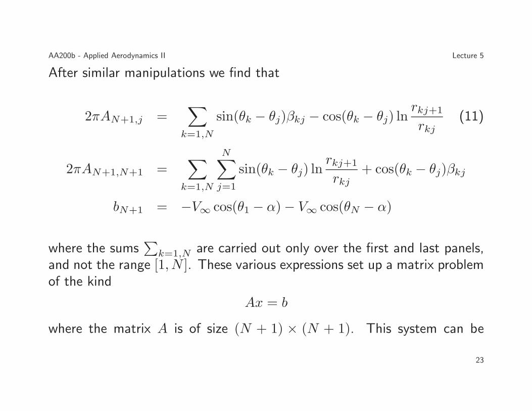
After similar manipulations we find that

2#AN+1,j ="

k=1,N

sin($k ! $j)(kj ! cos($k ! $j) lnrkj+1

rkj(11)

2#AN+1,N+1 ="

k=1,N

N"

j=1

sin($k ! $j) lnrkj+1

rkj+ cos($k ! $j)(kj

bN+1 = !V! cos($1 ! %) ! V! cos($N ! %)

where the sums(

k=1,N are carried out only over the first and last panels,and not the range [1, N ]. These various expressions set up a matrix problemof the kind

Ax = b

where the matrix A is of size (N + 1) $ (N + 1). This system can be

23


sketched as follows:)

******+

A11 . . . A1i . . . A1N A1,N+1... ... ... ...

Ai1 . . . Aii . . . AiN Ai,N+1... ... ... ...

AN1 . . . ANi . . . ANN AN,N+1

AN+1,1 . . . AN+1,i . . . AN+1,N AN+1,N+1

,

------.

)

******+

q1...qi...

qN

"

,

------.=

)

******+

b1...bi...

bN

bN+1

,

------.

Notice that the cost of inversion of a full matrix such as this one isO(N + 1)3, so that, as the number of panels increases without bounds,the cost of solving the panel problem increases rapidly. This is usually nota problem for two-dimensional flows, but becomes a serious problem inthree-dimensional flows where the number of panels, instead of being in theneighborhood of 100, is usually closer to 10, 000. Iterative solution methodsand panel method implementations using fast multipole methods can helpalleviate this problem. More on this later.

24


Finally, once you have solved the system for the unknowns of theproblem, it is easy to construct the tangential velocity at the midpoint ofeach panel according to the following formula

Vti = V! cos($i ! %) +N"

j=1

qj

2#

#sin($i ! $j)(ij ! cos($i ! $j) ln

rij+1

rij

$

+"

2#

N"

j=1

#sin($i ! $j) ln

rij+1

rij+ cos($i ! $j)(ij

$

And knowing the tangential velocity component, we can compute thepressure coe"cient (no approximation since Vni = 0) at the midpoint ofeach panel according to the following formula

Cp(xi, yi) = 1 ! V 2ti

V 2!

25


from which the force and moment coe"cients can be computed assumingthat this value of Cp is constant over each panel and by performing thediscrete sum. How close is the cd to zero? Try it in HW1.

26

Documents

Hess-Smith P anel Metho d - Stanford Universityadl.stanford.edu/aa210b/Lecture_Notes_files/Hess-Smith.pdf · Hess-Smith P anel Metho d AA200b L e c t u r e 5 Ap ril 7 , 2000 A A 200b