herd behavior and aggregate fluctuations in financial markets

Macroeconomic Dynamics, 4, 2000, 170–196. Printed in the United States of America.

HERD BEHAVIOR AND AGGREGATEFLUCTUATIONS IN FINANCIALMARKETS

RAMA CONTCentre de Mathematiques Appliquees, Ecole Polytechnique

JEAN-PHILIPE BOUCHAUDSPEC, Centre d’Etudes de Saclay

We present a simple model of a stock market where a random communication structurebetween agents generically gives rise to heavy tails in the distribution of stock pricevariations in the form of an exponentially truncated power law, similar to distributionsobserved in recent empirical studies of high-frequency market data. Our model provides alink between two well-known market phenomena: the heavy tails observed in thedistribution of stock market returns on one hand and herding behavior in financial marketson the other hand. In particular, our study suggests a relation between the excess kurtosisobserved in asset returns, the market order flow, and the tendency of market participants toimitate each other.

Keywords: Heavy Tails, Financial Markets, Herd Behavior, Market Organization,Intermittency, Random Graphs, Percolation

1. INTRODUCTION

Empirical studies of the fluctuations in the price of various financial assets haveshown that distributions of stock returns and stock price changes have fat tails thatdeviate from the Gaussian distribution [Mandelbrot (1963, 1997), Pagan (1996),Campbell et al. (1997), Cont et al. (1997), Guillaume et al. (1997), Pictet et al.(1997)] especially for intraday timescales [Cont et al. (1997)]. These fat tails,characterized by a significant excess kurtosis, persist even after accounting forheteroskedasticity in the data [Bollerslev et al. (1992)]. The heavy tails observedin these distributions correspond to large fluctuations in prices, “bursts” of volatilitythat are difficult to explain only in terms of variations in fundamental economicvariables [Shiller (1989)].

The fact that significant fluctuations in prices are not necesarily related to thearrival of information [Cutler (1989)] or to variations in fundamental economicvariables [Shiller (1989)] leads us to think that the high variability present in stock

R. Cont gratefully acknowledges an AMX fellowship from Ecole Polytechnique and thanks Science & Finance for theirhospitality. We thank Masanao Aoki, Alan Kirman, Dietrich Stauffer, and two anonymous referees for helpful remarksand Yann Braouezec for numerous bibliographical indications. Address correspondence to: Rama Cont, Centre deMathematiques Appliquées,Ecole Polytechnique, F-91128 Palaiseau, France; e-mail: [email protected].

c© 2000 Cambridge University Press 1365-1005/00 $9.50 170

HERD BEHAVIOR AND AGGREGATE FLUCTUATIONS 171

market returns may correspond to collective phenomena such as crowd effects or“herd” behavior.

Although herding in financial markets is by now relatively well documentedempirically, there have been few theoretical studies on the implications of herdingand imitation for the statistical properties of market demand and price fluctuations.In particular, some questions that one would like to have answered are: Howdoes the presence of herding modify the distribution of returns? What are theimplications of herding for relations between market variables such as order flowand price variability? These are some of the questions that have motivated ourstudy.

The aim of the present study is to examine, in the framework of a simple model,how the existence of herd behavior among market participants may generically leadto large fluctuations in the aggregate excess demand, described by a heavy-tailednon-Gaussian distribution. Furthermore, we explore how empirically measurablequantities such as the excess kurtosis of returns and the average order flow maybe related to each other in the context of our model. Our approach provides aquantitative link between the two issues discussed earlier: theheavy tailsobservedin the distribution of stock market returns on the one hand and theherd behaviorobserved in financial markets on the other hand.

The article is divided into four additional sections. Section 2 reviews well-knownempirical facts about the heavy-tailed nature of the distribution of stock returns andvarious models proposed to account for it. Section 3 presents previous empiricaland theoretical work on herding and imitation in financial markets in relation tothe present study. Section 4 discusses the statistical properties of excess demandresulting from the aggregation of a large number of random individual demandsin a market. Section 5 defines our model and presents analytical results. Section 6interprets the results in economic terms, compares them to empirical data anddiscusses possible extensions. Details of calculations are given in the appendices.

2. THE HEAVY-TAILED NATURE OF ASSET RETURN DISTRIBUTIONS

It is by now well known that the distribution of returns of almost all financialassets—stocks, indexes, and futures—exhibits a slow asymptotic decay that de-viates from a normal distribution. This is quantitatively reflected in the excesskurtosis, defined as

κ = µ4

σ 4− 3, (1)

whereµ4 is the fourth central moment andσ is the standard deviation of thereturns. The excess kurtosisκ should be zero for a normal distribution but rangesbetween 2 and 50 for daily returns [Campbell et al. (1997), Pagan (1996)] andis even higher for intraday data. Studies of the distribution of returns reveal thepresence of heavy tails, fatter than those of a normal distribution but thinner thana stable Pareto–Lévy distribution [Cont (1998)]. In some cases the tail has been

172 RAMA CONT AND JEAN-PHILIPE BOUCHAUD

represented by an exponential form [Cont et al. (1997)] and in other cases by apower law with tail index between 3 and 4 [Pagan (1996)].

2.1. Statistical Mechanisms for Generating Heavy Tails

Many statistical mechanisms have been put forth to account for the heavy tails ob-served in the distribution of asset returns. Well-known examples are Mandelbrot’sstable-Paretian hypothesis [Mandelbrot (1963)], the mixture-of-distributions hy-pothesis [Clark (1973)], and models based on conditional heteroskedasticity [Engle(1995)].

It is well known that in the presence of heteroskedasticity, the unconditionaldistribution of returns will have heavy tails. In most models based on heteroskedas-ticity, the process of return is assumed to be conditionally Gaussian: The shocksare “locally” Gaussian and the non-Gaussian character of the unconditional dis-tribution is an effect of aggregation. It is obtained by superposing a large numberof local Gaussian shocks. In this description, sudden movements in prices areinterpreted as corresponding to a high value of conditional variance.

On one hand, it has been shown that although conditional heteroskedasticitydoes lead to fat tails in unconditional distributions, ARCH-type models cannotfully account for the kurtosis of returns [Hsieh (1991), Bollerslev et al. (1992)].On the other hand, from a theoretical point of view, there is no a priori reasonto postulate that returns are conditionally normal: although conditional normalityis convenient for parameter estimation of the resulting model, nonnormal condi-tional distributions possess the same qualitative features as for volatility clusteringwhile accounting better for heavy tails. Gallant and Tauchen (1989) report signifi-cant evidence of both conditional heteroskedasticity and conditional nonnormalityin the daily NYSE value-weighted index. Similarly, Engle and Gonzalez-Rivera(1991) show that when a GARCH(1,1) model is used for the conditional varianceof stock returns the conditional distribution has considerable kurtosis, especiallyfor small-firm stocks. Indeed, several authors have proposed GARCH-type modelswith nonnormal conditional distributions [Bollerslev et al. (1992)].

Stable distributions [Mandelbrot (1963)] offer an elegant alternative to het-eroskedasticity for generating fat tails, with the advantage that they have a naturalinterpretation in terms of aggregation of a large number of individual contributionsof agents to market fluctuations: Indeed, stable distributions may be obtained aslimit distributions of sums of independent or weakly dependent random variables,a property that is not shared by alternative models. Unfortunately, the infinitevariance property of these distributions is not observed in empirical data: samplevariances do not increase indefinitely with sample size but appear to stabilize ata certain value for large enough data sets. We discuss stable distributions in moredetail in Section 4.

A third approach, first advocated by Clark (1973), is to model stock returns bya subordinated process, typically subordinated Brownian motion. This amountsto stipulating that through a “stochastic time change” one can transform the


complicated dynamics of the price process into Brownian motion or some othersimple process. It can be shown that, depending on the choice of the subordinator,one can obtain a wide range of distributions for the increments, all of which pos-sess heavy tails, that is, positive excess kurtosis. As a matter of fact, even stabledistributions may be obtained as a subordinated Brownian motion. In the originalapproach of Clark (1973), the subordinator was taken to be trading volume. Otherchoices that have been proposed are the number of trades [Geman and Ané (1996)]or other local measures of market activity. However, none of these choices for thesubordinator leads to a normal distribution for the increments of the time-changedprocess, indicating that large fluctuations in price may not be completely explainedby large fluctuations in trading volume or number of trades.

In short, although heteroskedasticity and time deformation partly explain thekurtosis of asset returns, they do not explain it quantitatively: Even after accountingfor these effects, one is left with an important residual kurtosis in the resultingtransformed time series. Moreover, these approaches consider the market as a“black box” and are not based on any microeconomic representation of the marketphenomenon generating the data that they attempt to describe.

2.2. Heavy Tails as Emergent Phenomena

The failure of purely statistical explanations to account for the presence of heavytails in the distribution of asset returns suggests the existence of a more fundamentalmarket mechanism, common to all speculative markets, that generates such heavytails.

Recent works by Bak et al. (1997), Lux (1998), and others have tried to explainthe heavy-tailed nature of return distributions as an emergent property in a marketwhere fundamentalist traders interact with noise traders. Bak et al. (1997) considerseveral types of trading rules and study the resulting statistical properties for thetime series of asset prices in each case. Computer simulations of their model doseem to yield fat-tailed distributions for asset returns, which at least qualitativelyresemble empirical distributions of stock returns, showing that the appearance offat-tailed distributions can be regarded as an emergent property in large markets.However, the model has two drawbacks: First, it is a fairly complicated model withmany ingredients and parameters and it is difficult to see how each ingredient of themodel affects the results obtained, which in turn diminishes its explanatory power.Second, the complexity of the model does not allow explicit calculations to beperformed, preventing the model parameters from being compared with empiricalvalues.

We present here an alternative approach, which, by modeling the communicationstructure between market agents as arandom graph, proposes a simple mechanismaccounting for some nontrivial statistical properties of stock price fluctuations.Although much more rudimentary and containing fewer ingredients than the modelproposed by Bak et al. (1997), our model allows for analytic calculations to beperformed, thus enabling us to interpret in economic terms the role of each of


the parameters introduced. The basic intuition behind our approach is simple:Interaction of market participants through imitation can lead to large fluctuationsin aggregate demand, leading to heavy tails in the distribution of returns.

3. HERD BEHAVIOR IN FINANCIAL MARKETS

In the popular literature, “crowd effects” often have been associated with largefluctuations in market prices of financial assets. Although well known to marketparticipants, they have been considered only recently in the econometrics litera-ture. On the theoretical side, a number of recent studies have considered mimeticbehavior as a possible explanation for the excessive volatility observed in financialmarkets [Bannerjee (1993), Orléan (1995), Shiller (1989), Topol (1991)].

3.1. Empirical Evidence

The existence of herd behavior in speculative markets has been documented by acertain number of studies: Scharfstein and Stein (1990) discuss evidence of herdingin the behavior of fund managers, Grinblatt et al. (1995) report herding in mutualfund behavior, and Trueman (1994) and Welch (1996) show evidence for herdingin the forecasts made by financial analysts. See also Golec (1997).

3.2. Theoretical Studies

On the theoretical side, several studies have shown that, in a market with noisetraders, herd behavior is not necessarily “irrational” in the sense that it may becompatible with optimizing behavior of the agents [Shleifer and Summers (1994)].Other motivations may be invoked for explaining imitation in markets, such as“group pressure” [Bikhchandani et al. (1992), Lux (1998), Scharfstein and Stein(1990)].

Various models of herd behavior have been considered in the literature, thebest-known approach being that of Bannerjee (1992, 1993) and Bikhchandaniet al. (1992). In these models, individuals attempt to infer a parameter from noisyobservations and decisions of other agents, typically through a Bayesian procedure,giving rise to “information cascades” [Bikhchandani et al. (1992)]. An importantfeature of these models is the sequential character of the dynamics: Individualsmake their decisions one at a time, taking into account the decisions of the indi-viduals preceding them. The model therefore assumes a natural way of orderingthe agents. This assumption seems unrealistic in the case of financial markets: Or-ders from various market participants enter the market simultaneously and it is theinterplay between different orders that determines aggregate market variables.1

Nonsequential herding has been studied in a Bayesian setting by Orléan (1995)in a framework inspired by the Ising model. Orléan considers a model of identicalagents making binary decisions in which any two agents have the same tendencyto imitate each other, and studies the resulting Bayesian equilibria. In terms of


aggregate variables, this model leads either to a Gaussian distribution when theimitation is weak or to a bimodal distribution with nonzero modes, which Orléaninterprets as corresponding to collective market phenomena such as crashes or pan-ics. In neither case does one obtain a heavy-tailed unimodal distribution centeredat zero, such as those observed for stock returns.2

The approach proposed in this paper is different from both approaches describedabove. Our model is different from those of Bannerjee (1992) and Bikhchandaniet al. (1992) in that herding is not sequential. The unrealistic nature of the results ofOrlean (1995) arises from the fact that all agents are assumed to imitate each otherto the same degree. We avoid this problem by considering the random formation ofgroups of agent who imitate each other but such that different groups of agents makeindependent decisions, which allows for a heterogeneous market structure. Morespecifically, our approach considers the interactions between agents as resultingfrom arandomcommunication structure, as explained in the next section.

4. AGGREGATION OF RANDOM INDIVIDUAL DEMANDS

Consider a stock market withN agents, labeled by an integer 1≤ i ≤ N, tradingin a single asset, whose price at timet will be denotedx(t). During each timeperiod, an agent may choose either to buy the stock, to sell it, or not to trade. Thedemand for stock of agenti is represented by a random variableφi , which can takethe values 0,−1, or+1: A positive value ofφi represents a “bull” an agent willingto buy stock; a negative value represents a “bear,” eager to sell stock; andφi = 0means that agenti does not trade during a given period. The random character ofindividual demands may be due either to heterogeneous preferences or to randomresources of the agents, or both. For example, random utility models studied inthe literature on discrete-choice theory of product differentiation lead to randomindividual demands, the distribution of which depends on the distribution specifiedfor the random utility functions of agents [Anderson et al. (1993)]. Alternatively,the random nature of individual demand may result from the application by theagents of simple decision rules, each group of agents using a certain rule. However,to focus on the effect of herding, we do not explicitly model the decision processleading to the individual demands; rather, we model the result of the decisionprocess as a random variableφi . In contrast with many binary choice models inthe microeconomics literature, we allow for an agent to be inactive, that is, not totrade during a given time periodt . This, as we shall see, is important for derivingour results.

Let us consider for simplification that, during each time period, an agent mayeither trade one unit of the asset or remain inactive. The demand of the agenti isthen represented byφi ∈ {−1, 0,+1}, with φi = −1 representing a sell order. Theaggregate excess demand for the asset at timet is therefore simply

D(t) =N∑

i=1

φi (t), (2)


given the algebraic nature ofφi . The marginal distribution of agenti ’s individualdemand is assumed to be symmetric:

P(φi = +1) = P(φi = −1) = a, P(φi = 0) = 1− 2a, (3)

such that the average aggregate excess demand is zero; that is, the market isconsidered to fluctuate around equilibrium. A value ofa< 1/2 allows for a finitefraction of agents not to trade during a given period.

We are concerned here with obtaining a result that could then be compared withactual market data, and the short-term excess demand is not an easily observablequantity. Also, most of the studies on the statistical properties of financial timeseries have been done on returns, log returns, or price changes. We therefore needto relate the aggregate excess demand in a given period to the return or price changeduring that period. The aggregate excess demand has an impact on the price of thestock, causing it to rise if the excess demand is positive and to fall if it is negative.A common specification, which is compatible with standardtatonnementideas, isto assume a proportionality between price change (or return) and excess demand:

1x = x(t + 1)− x(t) = 1

λ

N∑i=1

φi (t), (4)

whereλ is themarket depth: It is the excess demand needed to move the priceby one unit; it measure the sensitivity of price to fluctuations in excess demand.Equation (4) emphasizes the price impact of the order flow as opposed to otherpossible causes for price fluctuations. Although in the long run, economic factorsother than short-term excess demand may influence the evolution of the asset price,resulting in mean reversion or more complex types of behavior, we focus here onthe short-run behavior of prices, for example, on intraday timescales in the case ofstock markets, and so, this approximation seems reasonable.

The linear nature of this relation also may be questioned. Results reported byFarmer (1998) and others, based on the study of the price impact of blocks of ordersof different sizes sent to the market, seem to indicate a linear relationship for smallprice changes with nonlinearity arising when the size of blocks is increased [seealso Kempf and Korn (1997)]. Nevertheless, if the one-period return1x is anonlinear but smooth functionh(D) of the excess demand, then a linearization ofthe inverse demand functionh (a first-order Taylor-series expansion inD) showsthat equation (4) may still hold for small fluctuations of the aggregate excessdemand withh′(0)= 1/λ.

To evaluate the distribution of stock returns from equation (4), we need to knowthe joint distribution of the individual demands [φi (t)]1≤i≤N . Let us begin byconsidering the simplest case in which individual demandsφi of different agentsare independent and identically distributed random variables. We refer to thishypothesis as the “independent agents” hypothesis. In this case the joint distributionof the individual demands is simply the product of individual distributions, and


the price variation1x is a sum ofN i.i.d.r.v.’s with finite variance. When thenumber of terms in equation (4) is large, the central limit theorem applied to thesum in equation (4) tells us that the distribution of1x is well approximated by aGaussian distribution. Of course, this result still holds as long as the distributionof individual demands has finite variance.

This can be seen as a rationale for the frequent use of the normal distributionas a model for the distribution of stock returns. Indeed, if the variation of marketprice is seen as the sum of a large number of independent or weakly dependentrandom effects, then it is plausible that a Gaussian description will be a good one.

Unfortunately, empirical evidence tells us otherwise: The distributions both ofasset returns [Pagan (1996), Campbell et al. (1997)] and of asset price changes[Mandelbrot (1963, 1997), Cont (1997), Cont et al. (1997)] have been shownrepeatedly to deviate significantly from the Gaussian distribution, exhibiting fattails and excess kurtosis.

However, the independent-agent model is also capable of generating aggregatedistributions with heavy tails. Indeed, if one relaxes the assumption that the individ-ual demandsφi have a finite variance, then under the hypothesis of independence(or weak dependence) of individual demands, the aggregate demand—and there-fore the price change if we assume equation (4)—will have a stable (Pareto–Lévy)distribution. This is a possible interpretation for the stable-Pareto model proposedby Mandelbrot (1963) for the heavy tails observed in the distribution of the in-crements of various market prices. The infinite variance ofφi then reflects theheterogeneity of the market, for example, in terms of broad distribution of wealthof the participants as proposed by Levy and Solomon (1997).

Mandelbrot’s stable-Paretian hypothesis has been criticized for several reasons,one of them being that it predicts an infinite variance for stock returns, whichimplies in practice that the sample variance will increase indefinitely with samplesize, a property that is not observed in empirical data.

More precisely, a careful study of the tails of the distribution—both conditionaland unconditional—of increments for various financial assets shows that they haveheavy tails with a finite variance [Pagan (1996), Cont et al. (1997), Bounchaudand Potters (1997)]. Many distributions verify these conditions, and various para-metric families of distributions have been proposed and tested against market data[Campbell et al. (1997)]. A particular one proposed by the authors and others[Cont et al. (1997)] is the family of exponentially truncated stable distributions,a parametric family of infinitely divisible distributions with finite variance, whichinclude stable Lévy distributions as a limiting case. For such models, the tails ofthe density have the asymptotic form of an exponentially truncated power law:

p(1x) ∼|1x|→∞

C

|1x|1+µ exp

(− 1x

1x0

)(5)

The estimated exponent,µ,3 is found to be close to 1.5 (µ ' 1.4–1.6) for awide variety of stocks and market indexes [Bouchaud and Potters (1997)]. This


asymptotic form allows for heavy tails (excess kurtosis) without implying infinitevariance.

However, it is known that the central limit theorem also holds for certainsequences of dependent variables: Under various types ofmixing conditions[Billingsley (1975)], which are mathematical formulations of the notion of “weak”dependence, aggregate variables will still be normally distributed. Therefore, thenon-Gaussian and more generally nonstable character of empirical distributions,be it excess demand or the stock returns, not only demonstrates the failure of the‘independent-agent’ approach, but also shows that such an approach is nowhereclose to being a good approximation. The dependence between individual de-mands is an essential character of the market structure and may not be left outin the aggregation procedure; they cannot be assumed to be weak [in the senseof a mixing condition; Billingsley (1975)] anddo change the distribution of theresulting aggregate variable.

Indeed, the assumption that the outcomes of decisions of individual agents maybe represented as independent random variables is highly unrealistic. Such anassumption ignores an essential ingredient of market organization, namely, theinteractionandcommunicationamong agents.

In real markets, agents may form groups of various sizes, which then may shareinformation and act in coordination. In the context of a financial market, groupsof traders may align their decisions and act in unison to buy or sell; a differentinterpretation of a group may be an investment fund corresponding to the wealthof several investors but managed by a single fund manager.

To capture such effects, we need to introduce an additional ingredient, namely,the communication structure between agents. One solution would be to specifya fixed trading-group structure and then proceed to study the resulting aggregatefluctuations. Such an approach has two major drawbacks. First, a realistic marketstructure may require specifying a complicated structure of clusters and renderingthe resulting model analytically intractable. More important, the resulting patternof aggregate fluctuations will crucially depend on the specification of the marketstructure.

An alternative approach, suggested by Kirman (1983 and 1996), is to considerthe market communication structure itself as stochastic. One way of generating arandom market structure is to assume that market participants meet randomly andtrades take place when an agent willing to buy meets an agent willing to sell. Thisprocedure, called “random matching” by some authors [Ioannides (1990)], hasbeen considered previously in the context of the formation of trading groups byIoannides (1990) and in the context of a stock market model by Bak et al. (1997).

Another way is to consider that market participants form groups or “clusters”through a random matching process, but that no trading takes places inside a givengroup. Instead, members of a given group adopt a common market strategy (e.g.,they decide to buy or sell or not to trade) and different groups may trade with eachother through a centralized market process. The trading takes place among thegroups, not among group members. In the context of a financial market, clusters


may represent, for example, a group of investors participating in a mutual fund.This is the line that we follow in this paper.

5. PRESENTATION OF THE MODEL

More precisely, let us suppose that agents group together in coalitions orclustersand that, once a coalition has formed, all of its members coordinate their individualdemands so that all individuals in a given cluster have the same belief regardingfuture movements of the asset price. Using the framework described in the preced-ing section, we consider that all agents belonging to a given cluster will have thesame demandφi for the stock. In the context of a stock market, these clusters maycorrespond, for example, to mutual funds (e.g., portfolios managed by the samefund manager) or to herding among security analysts as in Trueman (1994) andWelch (1996). The right-hand side of equation (3) therefore can be rewritten as asum over clusters:

1x = 1

λ

k∑α=1

Wαφα(t) = 1

λ

nc∑α=1

Xα, (6)

whereWα is the size of clusterα, φα(t), is the (common) individual demand ofagents belonging to the clusterα, nc is the number of clusters (coalitions), andXα =φαWα.

One may consider that coalitions are formed through binary links betweenagents, a link between two agents meaning that they undertake the same actionon the market, that is, they both buy or sell stock. For any pair of agentsi andj , let pi j be the probability thati and j are linked together. Again, to simplify,we assume thatpi j = p is independent ofi and j : all links are equally probable.Then(N − 1)p denotes the average number of agents a given agent is linked to.Because we are interested in studying theN→∞ limit, p should be chosen insuch a way that(N − 1)p has a finite limit. A natural choice ispi j = c/N, anyother choice verifying the above condition being asymptotically equivalent to thisone. The distribution of coalition sizes in the market thus is specified completelyby a single parameter,c, which represents the willingness of agents to align theiractions. It can be interpreted as a coordination number, measuring the degree ofclustering among agents.

Such a structure is known as arandom graphin the mathematical literature Erdösand Renyi (1960), Bollobas (1985). In terms of random-graph theory, we consideragents as vertices of a random graph of sizeN, and the coalitions as connectedcomponents of the graph. Such an approach to communication in markets usingrandom graphs was first suggested in the economics literature by Kirman (1983)to study the properties of the core of a large economy. Random graphs also havebeen used in the context of multilateral matching in search equilibrium models byIoannides (1990). A good review of the applications of random-graph theory ineconomic modeling is given by Ioannides (1996).


The properties of large random graphs in theN→∞ limit were first studied byErdos and Renyi (1960). An extensive review of mathematical results on randomgraphs is given by Bollobas (1985). The main resullts of the combinatorial approachare given in Appendix A. One can show [Bollobas (1985)] that forc= 1 theprobability density for the cluster size distribution decreases asymptotically as apower law:

P(W) ∼W→∞

A

W5/2,

whereas for values ofc close to and smaller than 1 (0< 1− c¿ 1), the clustersize distribution is cut off by an exponential tail:

P(W) ∼W→∞

A

W5/2exp

[(1− c)W

W0

]. (7)

Forc = 1, the distribution has an infinite variance, whereas forc < 1 the variancebecomes finite because of the exponential tail. In this case the average size of acoalition is of order 1/(1− c) and the average number of clusters is then of orderN(1− c/2).

Setting the coordination parameterc close to 1 means that each agent tendsto establish a link with one other agent, which can be regarded as a reasonableassumption. This does not rule out the formation of large coalitions through succes-sive binary links between agents but prevents a single agent from forming multiplelinks, as would be the case in a centralized communication structure in which oneagent (the “auctioneer”) is linked to all of the others. As argued by Kirman (1983),the presence of a Walrasian auctioneer corresponds to such “star-like,” centralizedcommunication structures. We are thus excluding such a situation by construc-tion: We are interested in a market in which information is distributed and notcentralized, which corresponds more closely to the situations encountered in realmarkets. More precisely, the local structure of the market may be characterizedby the following result [Bollobas (1985)]: In the limitN →∞, the numberνi ofneighbors of a given agenti is a Poisson random variable with parameterc:

P(νi = ν) = e−c cν

ν!. (8)

A Walrasian auctioneerw would be connected to every other agent:νw = N − 1.The probability for having a Walrasian auctioneer therefore is given byN P(νw =N − 1), which goes to zero whenN →∞.

There are two different ways to represent a market as a collection of agentsclustered into small groups. The first is to consider the groups as “trading groups,”that is, groups of market agents trading among themselves, with little or no tradeamong different trading groups. Each trading group acts as a minimarket withits own price, supply, and demand. This approach, which is the one adopted byIoannides (1990), can be used to model price, dispersion for example. When ap-plied to a financial market, the connected components of the random graph then


represent groups of traders who buy and sell between themselves but have veryfew transactions with other groups of traders.

As pointed out earlier, our approach is different: Here, the trading takes placenot among members of a given group but between different clusters. A givenmarket cluster is characterized by its sizeWα and its “nature,” that is, whether themembers are buyers or sellers. This is specified by a variableφα ∈ {−1, 0, 1}. Itis reasonable to assume thatWα andφα are independent random variables: Thesize of a group does not influence its decision whether to buy or sell. The variableXα = φαWα then is distributed symmetrically with a mass of 1− 2a at the origin.Let

F(u) = P(Xα ≤ u|Xα 6= 0). (9)

Then, the distribution ofXα is given by

G(u) = P(Xα ≤ u) = (1− 2a)H(u)+ 2aF(u), (10)

whereH is a unit step function at 0 (Heaviside function). We shall assume thatFhas a continuous density,f , which decays asymptotically as in (7):

f (u) ∼|u|→∞

A

|u|5/2 e−(c−1)|u|

W0 . (11)

The expression for the price variation1x therefore reduces to a sum ofnc i.i.d.r.v.’sXα, α = 1 . . .nc with heavy-tailed distributions as in (7):

1x = 1

λ

nc∑α=1

Xα.

Since the probability density ofXα has a finite mass 1−2a at zero, only a fraction2a of the terms in the sum (6) are nonzero; the number of nonzero terms in the sumis of order 2anc ∼ 2aN(1− c/2) = norder(1− c/2), wherenorder= 2aN is theaverage number of market participants who actively trade in the market during agiven period. For example,nordercan be thought of as the number of orders receivedduring the time period [t, t + 1] if we assume that different orders correspond tonet demands, as defined earlier, of different clusters of agents. For a time periodof, say, 15 min on a liquid market such as NYSE,norder= 100 is a typical orderof magnitude.

The distribution of the price variation1x is then given by

P(1x = u) =N∑

k=1

P(nc = k)k∑

j=0

(kj

)(2a) j (1− 2a)k− j f ⊗ j (λu), (12)

where⊗ denotes a convolution product,nc being the number of clusters. Equa-tion (12) enables us to calculate the moment-generating functionsF of the


aggregate excess demandD in terms of f (see Appendix C for details):

F(z) ∼N→∞

exp

{norder

(1− c

2

)[ f (z)− 1]

}. (13)

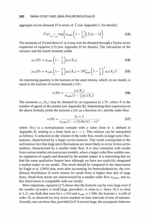
The moments ofD (and those of1x) may now be obtained through a Taylor-seriesexpansion of equation (13) (see Appendix D for details). The calculation of thevariance and the fourth moment yields

µ2(D) = norder

(1− c

2

)µ2(Xα), (14)

µ4(D) = norder

(1− c

2

)µ4(Xα)+ 3N2

order

(1− c

2

)2

µ2(Xα)2. (15)

An interesting quantity is the kurtosis of the asset returns, which, in our model, isequal to the kurtosis of excess demandκ(D):

κ(D) = µ4(Xα)

norder(1− c

2

)µ2(Xα)

. (16)

The momentsµ j (Xα) may be obtained by an expansion in 1/N, whereN is thenumber of agents in the market (see Appendix B). Substituting their expression onthe above formula yields the kurtosisκ(D) as a function ofc and the order flow:

κ(D) = 2c+ 1

norder(1− c/2)A(c)(1− c)3, (17)

where A(c) is a normalization constant with a value close to 1, defined inAppendix B, tending to a finite limit asc→ 1. This relation can be interpretedas follows: A reduction in the volume of the order flow results in larger price fluc-tuations, characterized by a larger excess kurtosis. This result corresponds to thewell-known fact that large price fluctuations are more likely to occur in less activemarkets, characterized by a smaller order flow. It is also consistent with resultsfrom various market microstructure models, where a larger order flow enables eas-ier regulation of supply and demand by the market maker. It is interesting that wefind the same qualitative feature here although we have not explicitly integrateda market maker in our model. This result should be compared to the observationby Engle et al. (1991) that, even after accounting for heteroskedasticity, the con-ditional distribution of stock returns for small firms is higher than that of largefirms. Small-firm stocks are characterized by a smaller order flownorders, and so,this observation is compatible with our results.

More important, equation (17) shows that the kurtosis can be very largeeven ifthe number of orders is itself large, providedc is close to 1. SinceA(1) is closeto 1/2, one finds that even forc= 0.9 andnorder= 1,000, the kurtosisκ is still oforder 10, as observed on very active markets on time intervals of tens of minutes.Actually, one can show that, provided 2aN is not too large, the asymptotic behavior


of P(1x) is still of the form given by equation (7). This model thus leads naturallyto the value ofµ = 3/2, close to the value observed on real markets. Of course,the value ofc could itself be time dependent. For example, herding tends to bestronger during periods of uncertainty, leading to an increase in the kurtosis. Whenc reaches 1, a finite fraction of the market simultaneously shares the same opinionand this leads to a crash. An interesting extension of the model would be one inwhich the time evolution of the market structure is explicitly modeled, and thepossible feedback effect of the price moves on the behavior of market participants.

6. SUMMARY AND RESULTS

We have presented a model of a speculative market withN agents who face threealternatives at each time period: to buy a unit of a financial asset, to sell a unitof the asset, or not to trade. We assume that the agents organize into groupsby forming independent binary links between each other with probabilityc/N,where 1< c< 1 is a connectivity parameter. The resulting market structure is thendescribed by a random graph withN vertices whose connected components orclusterscorrespond to groups of investors who pool their capital into a single fundor act in unison to buy or sell. Each cluster of agents now decides, independentlyfrom other clusters, whether to buy, to sell, or not to trade. To model this, weattribute to each cluster4 α a random variableφα taking values in{−1, 0,+1},with φα independent fromφβ if α 6=β. All agents belonging to the cluster areassumed to make the same decision: buy ifφα =+1, sell ifφα =−1, and not tradeif φα = 0. The variablesφα, where the indexα denotes clusters, are independentvariables with a symmetric distribution:

P(φα = +1) = P(φα = −1) = a, P(φα = 0) = 1− 2a. (18)

As explained earlier,norder = 2aN represents the average order flow (numberof orders per unit time arriving on the market), which should remain finite in theN →∞ limit, meaning that only a finite number of agents are allowed to trade atthe same time. This leads us to parameterizea as

a = norder

2N+ o

(1

N

). (19)

Denotingφi (t)∈ {−1, 0,+1} as the demand of agenti , the above statements implythat

φi andφ j are independent random variables ifi and j do not belong to the same cluster;φi = φ j otherwise.

The variablesφi , i ∈ [1, N] together with the graph structure defined by the linksdefines the configuration of the market. LetM be such a configuration,L(M)

be the number of links inM, C−(M) be the number of clustersα with φα =−1(clusters of sellers),C+(M) be the number of clustersα with φα =+1 (clusters of


buyers), andC0(M) be the number of clustersα with φα = 0 (nontrading clusters).Then, according to our specifications, such a market configuration is observed withprobability

P(M) =(

c

N

)L(M)(1− c

N

)(N2)−L(M)(

1− norder

N

)C0(M)(norder

N

)C+(M)+C−(M)

.

The excess demandD(t)= ∑φi (t) then gives rise to a change1x(t) in themarket price, which is assumed to be linearly related toz(t) [equation (4)]. We areinterested in the distribution of1x(t) or, equivalently, ofD(t) (more precisely,its tail behavior) in the above model, when the numberN of investors is large. Tostudy this limit, we assume thatc< 1 and that the order flownordersremains finitewhenN→∞. Under these assumptions (see Appendix C),

(1) The density of price changes1x displays a heavy, non-Gaussian tail of the form

p(u) ∼|u|→∞

eu

u0

u5/2. (20)

(2) The heaviness of the tails, as measured by the kurtosis of the price change, is inverselyproportional to the order flow:

κ(1x) = 2c+ 1

norder

(1− c

2

)A(c)(1− c)3

. (21)

This means that an illiquid market—that is, with a weak order flow—will producelarge price fluctuations with higher frequency than a market in which there aremore orders flowing in per unit time.

The quantities above are defined for a certain time interval1t , taken to beunity in the relations above. Changing the time interval would modify, among allof the parameters defining the model, only the order flownorders, which shouldbe an increasing function of the time interval1t . Equation (13) then impliesthat, as the time interval1t increases, the price changes over1t become moreand more Gaussian, which is indeed consistent with empirical observations [Contet al. (1997)]. Our model thus enables a crossover between heavy tails at smalltimescales and Gaussian behavior of price increments at large timescales, thecrossover being caused by the increase of number of orders during1t when1tis increased. More precisely, this remark together with equation (21) implies alink between the scaling behavior of the kurtosis of price increments on timescale1t and the manner in which the order flow during1t should increase with1t .Recent empirical studies [Cont (1997)] have suggested that the kurtosis of priceincrements on timescale1t exhibits a nonlinear (anomalous) scaling behavior,

κ ∼ |1t |−α, (22)

withα' 0.4. As shown by Cont (1997), this observation is consistent with a power-law decay in the correlation function of squared price changes, a well-documentedproperty of stock returns. In view of equation (21), this would imply that the order


flow during1t should increase as|1t |α, a prediction that can be tested empirically.Note that a somewhat similar scaling relation for the trading volume as a functionof1t was proposed by Clark (1973), but our assertion is of a different nature sinceClark’s relation concerned trading volume and not order flow.

7. DISCUSSION

We have exhibited a model of a stock market that, albeit its simplicity, givesrise to a probability distribution with heavy tails and finite variance for aggregateexcess demand and stock price variations, similar to empirical distributions of assetreturns. Our model illustrates the fact that whereas a naive market model in whichagents do not interact with each other would tend to give rise to normally distributedaggregate fluctuations, taking into account interaction between market participantsthrough a rudimentary herding mechanism gives a result that is quantitativelycomparable to empirical findings on the distribution of stock market returns.

7.1. Link Between Herd Behavior and Price Intermittency

One of the interesting results of our model is that it predicts a relation betweenthe fatness of the tails of asset returns as measured by their excess kurtosis andthe degree of herding among market participants as measured by the parameterc.This relation is given by equation (17) .

Although we implicitly assumed thatt represents chronological time, we couldformulate the model by consideringt as market time, leading to a subordinatedprocess in real time as in Clark (1973), with the difference that the underlyingprocess will not be a Gaussian random walk.

7.2. Levels of Randomness

As explained earlier, the structure of the market is described in our model as arandom graph. On this random market structure is superimposed another sourceof randomness, that of the demands of agents of each group. Note that these twosources of randomness are not of the same nature. First, whereas a given herdmay rapidly switch from buying to selling on a very short timescale, the structureof herds (i.e. the market structure) is likely to evolve much more slowly in time.Therefore, there is a separation between slow variables (the herd sizesWi ) and fastvariables (φi ). if we are interested in dynamics on short timescales, of the orderof an hour in a liquid market, we can consider the market structure as essentiallystatic; this is not true, however, in the long run.

7.3. Robustness with Respect to Market Topology

When defining interactions between market participants, one needs a notion ofdistance between different agents. Contrary to the case of physical systems, such


a notion is not readily available in socioeconomic systems, and the results of agiven model may depend heavily on how neighborhood relations are defined. Inthe above model, we allow agents to choose their “neighbors” randomly, whichamounts to using a random graph topology for the market communication structure[Kirman (1983)]. One might wonder how sensitive the results of the model are tothis specification. Stauffer and Penna (1998) have simulated variants of our modelin which the agents are placed on ad-dimensional lattice and form random linksonly with their nearest neighbors as defined by the lattice topology. Interestingly,their extensive Monte-Carlo simulations for various lattice sizes and dimensions(d= 2 to 7) show that the results of Section 6 remain true and therefore do notcrucially depend on the graph structure specified above, which is not obvious apriori.

7.4. Extensions

Our model raises several interesting questions. As remarked earlier, the value ofcis specified as being less than, and close to 1. Fine-tuning a parameter to a certainvalue may seem arbitrary unless one can justify such an assumption. An interestingextension of the model would be one in which the time evolution of the marketstructure is explicitly modeled in such a way that the parameterc remains in thecritical region (close to 1). Note, however, that our results are not restricted to asingle value ofc but to a whole range of values< 1.

One approach to this problem is via the concept of “self-organized criticality,”introduced by Bak et al. (1987): Certain dynamical systems generically evolve toa state where the parameters converge to the critical values, leading to scaling lawsand heavy-tailed distributions for the quantities modeled. This state is reachedasymptotically and is an attractor for the dynamics of the system. Bak et al. (1993)present a simple model of an economic system presenting self-organized criticality(see also Lux and Marchesi (1999)).

Note, however, that for the above results to hold, one does not need to adjustc to a critical value: It is sufficient forc to be within a certain range of values.As noted earlier, whenc approaches 1 the clusters become larger and larger and agiant coalition appears whenc ≥ 1. In our model the activation of such a clusterwould correspond to a market crash (or boom). To be realistic, the dynamicsof c should be such that the crash (or boom) isnot a stable state and the giantcluster disaggregates shortly after it is formed: After a short period of panic, themarket resumes normal activity. In mathematical terms, one should specify thedynamics ofc(t) such that the valuec = 1 is “repulsive.” This can be achieved byintroducing a feedback effect of prices on the behavior of market participants: Anonlinear coupling between can lead to a control mechanism maintainingc in thecritical region.

Yet another interesting dynamical specification compatible with our modelis obtained by considering agents with “threshold response.” Threshold modelshave been considered previously as possible origins for collective phenomena in


economic systems [Granovetter (1983)]. One can introduce heterogeneity by al-lowing the individual thresholdθi to be random variables: For example, one mayassume theθi ’s to be i.i.d. with a standard deviationσ(θ). A simple way to in-troduce interactions among agents is through an aggregate variable: Each agentobserves the aggregate excess demandD(t) given by equation (2) or eventuallyD(t)+E(t), whereE is an exogeneous variable. Agents then evolve as follows: Ateach time step, an agent changes its market positionφ(t) (“flips” from long to shortor vice versa) if the observed signalD(t) crosses his or her thresholdθi . Aggregatefluctuations then can occur through cascades or “avalanches” corresponding to theflipping of market positions of groups of agents. This model has been studied inthe context of physical systems by Sethna et al. (1997), who have shown that, fora fairly wide range of values ofσ(θ), one observes aggregate fluctuations whosedistribution has power-law behavior with exponential tails, as in equation (7).

These issues will be adressed in a forthcoming work.

NOTES

1. Bikhchandani et al. (1992) do not consider their model applicable to financial markets, but foranother reason: They remark that as the herd grows, the cost of joining it will also grow, discourag-ing new agents from joining. This aspect, which is not taken into account by their model, is againunavoidable in the sequential character of herd formation.

2. Note, however, that one could also obtain heavy tails in Orléan’s approach by placing the systemat the critical temperature of the corresponding Ising model.

3. Because of the presence of the exponential, this exponent isnot the same as the Hill estimatoror the one found by fitting a power law to the tails of return distributions. Moreover, it is easy to seethat several functional forms can have the same behavior in some ranges of values; we do not claimthat the functional form (5) has any canonical feature to it but that it fits the empirical data well.

4. Greek subscripts denote clusters and Roman subscripts denote the agents.

REFERENCES

Anderson, S.P., A. de Palma & J.F. Thisse (1993)Discrete Choice Theory of Product Differentiation.Cambridge, MA: MIT Press.

Bak, P., C. Tang & K. Wiesenfeld (1987) Self-organized criticality.Physical Review Letters59, 381–387.

Bak, P., K. Chen, J. Scheinkman & M. Woodford (1993) Aggregate fluctuations from independentsectorial shocks: Self-organized criticality in a model of production and inventory dynamics.RicercheEconomichi47, 3–30.

Bak, P., M. Paczuski & M. Shubik (1997) Price variations in a stock market with many agents.PhysicaA 246, 430–440.

Bannerjee, A. (1992) A simple model of herd behavior.Quarterly Journal of Economics107, 797–818.Bannerjee, A. (1993) The economics of rumours.Review of Economic Studies60, 309–327.Bikhchandani, S., D. Hirshleifer & I. Welch (1992) A theory of fads, fashion, custom and cultural

changes as informational cascades.Journal of Political Economy100, 992–1026.Billingsley, P. (1975)Convergence of Probability Measures. New York: Wiley.Bollerslev, T., R.C. Chou & K. Kroner (1992) ARCH modeling in finance.Journal of Econometrics

52, 5–59.Bollobas, B. (1985)Random Graphs. New York: Academic Press.Bouchaud, J.P. & M. Potters (1997)Theorie des Risques Financiers. Paris: Alea Saclay.


Campbell, J., A.H. Lo & C. McKinlay (1997)The Econometrics of Financial Markets. Princeton, NJ:Princeton University Press.

Clark, P.K. (1973) A subordinated stochastic process model with finite variance for speculative prices.Econometrica41, 135–155.

Cont, R. (1997) Scaling and Correlation in Financial Time Series. Science & Finance working paper.Cont, R. (1998)Statistical Finance: Empirical and Theoretical Study of Price Variations in Financial

Markets, Ph.D. dissertation, Université de Paris XI.Cont, R., M. Potters & J.P. Bouchaud (1997) Scaling in stock market data: Stable laws and beyond. In

B. Dubrulle, F. Groner & D. Sornette (eds.),Scale Invariance and Beyond. Berlin: Springer.Cutler, D.M., J.M. Poterba & L. Summers (1989) What moves stock prices?Journal of Portfolio

Management(Spring), 4–12.Engle, R. (1995)ARCH: Selected Readings. Oxford: Oxford University Press.Engle, R. & A. Gonzalez-Rivera (1991) Semiparametric ARCH models.Journal of Business and

Statistics9, 345–360.Erdos, P. & A. Renyi (1960) On the evolution of random graphs.Publications of the Mathematical

Institute of the Hungarian Academy of Sciences5, 17–61.Farmer, D. (1998) Market force, ecology and evolution. http://xxx.lpthe.jussieu.fr/abs/adap-org/

9812005.Feller, W. (1950)Introduction to Probability Theory and Its Applications, vol. II, 3rd ed. New York:

Wiley.Gallant, A.R. & G. Tauchen (1989) Semi nonparametric estimation of conditional constrained hetero-

geneous processes.Econometrica1091–1120.Geman, H. & T. Ane (1996) Stochastic subordination.RISK(September).Golec, J. (1997) Herding on noise: The case of Johnson Redbook’s weekly retail sales data.Journal of

Financial and Quantitative Analysis32(3), 367–400.Granovetter, M. & R. Soong (1983) Threshold models of diffusion and collective behavior.Journal of

Mathematical Sociology9, 165–179.Grinblatt, M., S. Titman S. & R. Wermers (1995) Momentum investment strategies, portfolio perfor-

mance and herding: A study of mutual fund behavior.American Economic Review85, 1088–1104.Guillaume, D.M., M.M. Dacorogna, R.R. Davé, U.A. Muller, R.B. Olsen and O.V. Pictet (1997) From

the birds eye to the microscope: A survey of new stylized facts of the intra-day foreign exchangemarkets.Finance and Stochastics1, 95–130.

Hsieh, D.A. (1991) Chaos and non-linear dynamics: Application to financial markets.Journal ofFinance46, 1839–1877.

Ioannides, Y.M. (1990) Trading uncertainty and market form.International Economic Review31,619–638.

Ioannides, Y.M. (1996) Evolution of trading structures. In B.W. Arthur, D. Lane & S.N. Durlauf (eds.),The Economy as an Evolving Complex System. Redwood Hill, CA: Addison Wesley.

Kempf, A. & O. Korn (1997) Market Depth and Order Size. Lehrstuhl für Finanzierung working paper97-05, Universität Mannheim.

Kirman, A. (1983) Communication in markets: A suggested approach.Economics Letters12, 1–5.Kirman, A. (1996) Interaction and Markets. GREQAM working paper.Levy, M. & S. Solomon (1997) New evidence for the power law distribution of wealth.Physica A242,

90–94.Lux, T. (1998) The socio-economic dynamics of speculative markets.Journal of Economic Behavior

and Organization33, 143–165.Lux, T. & M. Marchesi (1999) Scaling and criticality in a stochastic multi-agent model of a financial

market.Nature397.Mandelbrot, B. (1963) The variation of certain speculative prices.Journal of Business36, 392–417.Mandelbrot, B. (1997)Fractals and Scaling in Finance. Berlin: Springer.Orlean, A. (1995) Bayesian interactions and collective dynamics of opinion.Journal of Economic

Behavior and Organisation28, 257–274.


Pagan, A. (1996) The econometrics of financial markets.Journal of Empirical Finance3, 15–102.Pictet, O.V., M. Dacorogna, U.A. Muller, R.B. Olsen & J.R. Ward (1997) Statistical study of foreign

exchange rates, empirical evidence of a price change scaling law and intraday analysis.Journal ofBanking and Finance14, 1189–1208.

Scharfstein, D.S. & J.C. Stein (1990) Herd behavior and investment.American Economic Review80,465–479.

Sethna, J.P., O. Perkovic & K. Dahmen (1997) Hysteresis, avalanches and Barkhausen noise. In B.Dubrulle, F. Groner & D. Sornette (eds.),Scale Invariance and Beyond. Berlin: Springer.

Shiller R. (1989)Market Volatility. Cambridge, MA: MIT Press.Shleifer, A. & L.H. Summers, Crowds and Prices: Towards a Theory of Inefficient Markets. Working

paper 282, University of Chicago Center for Research in Security Prices.Stauffer, D. & T.J.P. Penna, (1998) Crossover in the Cont-Bouchaud percolation model for market

fluctuations.Physica A256, 284–290.Topol, R. (1991) Bubbles and volatility of stock prices: Effect of mimetic contagion.Economic Journal

101, 786–800.Trueman, B. (1994) Analysts forecasts and herding behavior.Review of Financial Studies7, 97–124.Welch, Ivo (1996) Herding Among Security Analysts. Working paper 8-96, University of California

at Los Angeles.

APPENDICES

Unless specified otherwise,f (N, c)∼ g(N, c) means

f (N, c)

g(N, c)= 1+ o

N→∞(1)

uniformly in c on all compact subsets of ]0,1[.

APPENDIX A: SOME RESULTS FROMRANDOM GRAPH THEORY

In this appendix, we review some results on asymptotic properties of large random graphs.Proofs for most of the results can be found in Erdös and Renyi (1960) or Bollobas (1985).

ConsiderN labeled pointsV1,V2, . . .VN , calledvertices. A link (or edge) is defined asan unordered pair{i , j }. A graph is defined by a setV of vertices and a setE of edges. Anytwo vertices may either be linked by one edge or not be linked at all. In the language ofgraph theory, we consider non-oriented graphs without parallel edges. We always denotethe number of vertices byN. A path is defined as a finite sequence of links such that everytwo consecutive edges and only these have a common vertex. Vertices along a path can belabeled in two ways, thus enabling us to define the extremities of the path. A graph is said


to be connected if any two verticesVi ,Vj are linked by a path; that is, there exists a pathwith Vi andVj as extremities. Acycle(or loop) is defined as a path such that the extremitiescoincide. A graph is called atree if it is connected and if none of its subgraphs is a cycle.A graph is called acyclic if all of its subgraphs are trees.

Consider now a graph built by choosing, for each pair of verticesVi ,Vj , whether to linkthem or not through a random process, the probability for selecting any given edge beingp> 0, the decisions for different edges being independent. A graph obtained by such aprocedure is termed arandom graphof typeG(N, p) in the notations of Bollobas (1985).This definition corresponds to random graphs of type0∗∗n,N in Erdos and Ranyi (1960, p. 20).

In the following, we are specifically interested in the casep= c/N. Various graph-theoretical parameters of such graphs are random variables whose distributions only dependson N andc. We are particularly interested in the properties of large random graphs of thistype, that is,G(N, c/N) in the limit N →∞.

The following results have been shown by Erdös and Renyi (1960) and Bollobas (1985):If c< 1, then in the limitN→∞ all points of the random graphs belong to trees exceptfor a finite numberU of vertices, which belong to unicyclic components. Moreover, theprobability of a vertex belonging to a cyclic component tends to zero asN−1/3. For describingthe structure of large random graphs forc< 1, it is therefore sufficient to account for verticesbelonging to trees; cyclic components do not essentially modify the results, except whenc= 1.

More precisely [Bollobas (1985, Theorem V.22)],

U ∼ 1

2

∞∑k=3

(ce−c)kk−3∑j=0

k j

j !,

σ 2(U ) ∼ 1

2

∞∑k=3

k(ce−c)kk−3∑j=0

k j

j !.

The preceding expressions are valid forc 6= 1.

APPENDIX B: DISTRIBUTION OF CLUSTERSIZES IN A LARGE RANDOM GRAPH

Let p1(s) be the probability for a given vertex to belong to a cluster of sizes in theN →∞limit. The moment-generating function81 of the p1 is defined by

81(z) =∞∑

s=1

eszp1(s).

We now proceed to derive a functional equation verified by81 in the largeN limit whenthe effects of loops (cycles) are neglected.


Let p1N(s) be the corresponding probability in a random graph withN vertices. Adding

a new vertex to the graph will modify the pattern of links, the probability ofk new linksfrom the new vertex to the old ones being(

c

N

)k(1− c

N

)N−k(N

k

).

As shown in Appendix A, the probability of creating a cycle tends to zero for largeN. Theconstraint that no new cycles be created by the new links imposes the condition that thek links are made to vertices ink different clusters of sizes. Ifs1, s2, . . . sk are the sizes ofthese clusters, then the new links will create a new cluster of sizes1 + s2 + · · · + sk + 1:

p1N+1(s) =

N∑k=1

N∑s1,...,sk=1

(N

k

)(c

N

)k(1− c

N

)N−k

× δ(s1 + s2 + · · · + sk + 1− s)p1N(s1)p

1N(s2) . . . p1

N(sk).

Multiplying both sides byesz and summing overs gives

81(z, N + 1) = ez

[1+ c

N+81(z, N)

c

N

]N

,

which gives, in the largeN limit,

81(z) = ez+c(81(z)−1),

from which various moments and cumulants may be calculated recursively. The distributionof cluster sizesp(s) is then given by

p(s) = A(c)p1(s)

s,

whereA(c) is a normalizing constant defined such that∫

p(s) ds= 1.

APPENDIX C: NUMBER OF CLUSTERSIN A LARGE RANDOM GRAPH

Let nc(N) be the number of clusters (connected components) in a random graph of sizeN defined as above;nc is a random variable whose characteristics depend onN and theparameterc. In this section, we show thatnc has an asymptotic normal distribution whenN →∞ and that for largeN, the j th cumulantCj of nc is given by

Cj ∼N→∞

(−1) j Nc

2.


From a well-known generalization of Euler’s theorem in graph theory,

l (N)− N + nc(N) = χ(N),

whereχ(N) is the number of independent cycles andl (N) is the number of links. Thisimplies in turn that

nc(N) = N

(1− c

2

)+ O(1)

We retrieve this result later and proceed to calculate higher moments via an approximation.Define the moment-generating function for the variablenc(N) to be

8N(z, c) = encz =N∑

k=1

PN,c(nc = k)ekz.

The j th moment ofnc is then given by

ncj = ∂ jφN

∂zj(0, c).

Let us also consider the cumulant generating function9 defined by8(z) = exp9(z). Thej th cumulantof the distribution ofnc then can be calculated as

Cj (N, c) = ∂ j9N

∂zj(0, c).

We now establish an approximate recursion relation between8N and8N+1. Take a randomgraph of sizeN, the probability of a link between any two vertices beingp = c/N. To obtaina graph withN+ 1 vertices, add a new vertex and choose randomly the links between the newvertex and the others. Note that since in a graph of sizeN the link probability ispN = c/N,our new graph will correspond to a graph of sizeN+1 with parameterc′ = c(N+1)/N sothat the link probability isc′/(N + 1)= c/N. We assume that the probability of two linksbeing made to the same cluster is negligible, that is, that no cycles are created by the newlinks, which is a reasonable approximation given the results in Appendix A. In this case,eachk links emanating from the new vertex will diminish the number of clusters byk− 1,giving the following recursion relation:

PN+1,c′(n) =(

1− c

N

)N

PN+1,c′(n+ 1)

+N∑

k=1

(N

k

)(c

N

)k(1− c

N

)N−k

PN+1,c′(n+ k− 1).

Multiplying each side byenz and summing overn = 1 . . . N gives

8N+1(z, c′) = ez8N(z, c)

[1+ c

N(e−z − 1)

]N


or, in terms of the cumulant-generating function9N ,

9N+1

[z, c

(1+ 1

N

)]= z+9N(z, c)+ ln

[1+ c

N(e−z − 1)

]N

. (C.1)

WhenN →∞, a first-order expansion in 1/N gives

8N+1(z, c)+ c

N∂28N+1(z, c)

= ez8N(z, c) exp

{c(e−z − 1)

[1− c2(e−z − 1)2

N

]}+ o

(1

N

), (C.2)

where∂2 denotes a partial derivative with respect to the second variable. The second termon the left-hand side stems from the expansion in the variablec′ = c(1+1/N) and reflectsthe fact that the probability for a link has to be renormalized when going from anN-graphto a (N+ 1)-graph.

By taking successive partial derivatives of (C.1) and (C.2) with respect toz, one then canderive the recursion relation for the moments and cumulants ofnc. Let us first retrieve theresult given in Appendix A fornc. Defineγ (c) such that

nc = ∂φN

∂z(0, c) = γ1(c)N + O(1).

Substituting in (C.1) yields a simple differential equation forγ1:

γ1(c)+ cγ1′(c) = 1− c,

whose solution isγ1(c) = (1− c/2), that is,

nc =(

1− c

2

)N + O(1),

nc

N→ 1− c

2.

Let us now derive a similar relation for the varianceσ 2(N, c) = var(nc). Let

σ 2(N, c) = γ2(c)N + O(1).

By taking derivatives twice with respect toz in (C.1) and settingz = 0, we obtain, up tofirst order in 1/N,

γ2(c)+ cγ2′(c) = c,

whenceγ2(c) = c/2. By calculating thej th derivative in (C.1) with respect toz, we canderive in the same way an asymptotic expression for thej th cumulant ofnc:

Cj ∼N→∞

(−1) j Nc

2.

Note that the asymptotic forms for cumulants ofnc are identical to those of a randomvariableZ with the following distribution:

P(Z = k) =

(Nc

2

)N−k

(N − k)!e−

Nc2 ;


that is,N−Z is a Poisson variable with parameterNc/2. Without rescaling, this distributionbecomes degenerate in the largeN limit. Nevertheless, for finiteN, both8N and9N areanalytic functions ofz in a neighborhood of zero. Consider now the rescaled variable:

YN =nc − N

(1− c

2

)√

Nc/2.

YN has zero mean and unit variance and its higher cumulants tend to zero:

∀ j ≥ 3, Cj (YN) →N→∞

0.

The standard normal distribution is the only distribution with zero mean, unit variance,and zero higher cumulants. Under these conditions, we can show [Feller (1950)] that theconvergence of the cumulants implies convergence in distribution:

nc − N(1− c

2

)√

Nc/2∼

N→∞N (0, 1).

APPENDIX D: DISTRIBUTION OFAGGREGATE EXCESS DEMAND

In this appendix, we derive an equation for the generating function of the variable1x,which represents in our model the one-period return of the asset. The relation between1xand other variables of the model is given by equation (6):

1x = 1

λ

nc∑α=1

Wαφα = 1

λ

nc∑α=1

Xα,

wherenc is the number of clusters or trading group, that is, the number of connectedcomponents of the random graph in the context of our model. The number of clustersnc isitself a random variable, whose cumulants are known in theN →∞ limit (see Appendix C).As for the random variablesXα, their distribution is given by equation (10):

P(1x = x) =N∑

k=1

P(nc = k)k∑

j=0

(kj

)(2a) j (1− 2a)k− j f ⊗ j (λx).

To calculate this sum, let us introduce the moment-generating functions for1x andX′α:

f (z) =∑

s

f (s)esz, F(z) =∑

s

P(λ1x = s)esz.


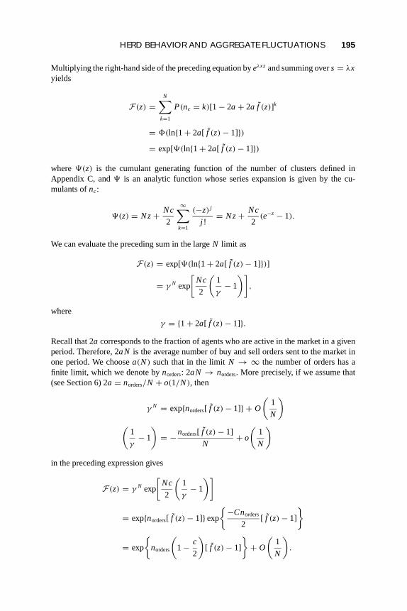
Multiplying the right-hand side of the preceding equation byeλxz and summing overs= λxyields

F(z) =N∑

k=1

P(nc = k)[1− 2a+ 2a f (z)]k

= 8(ln{1+ 2a[ f (z)− 1]})= exp[9(ln{1+ 2a[ f (z)− 1]})

where9(z) is the cumulant generating function of the number of clusters defined inAppendix C, and9 is an analytic function whose series expansion is given by the cu-mulants ofnc:

9(z) = Nz+ Nc

2

∞∑k=1

(−z) j

j != Nz+ Nc

2(e−z − 1).

We can evaluate the preceding sum in the largeN limit as

F(z) = exp[9(ln{1+ 2a[ f (z)− 1]})]

= γ N exp

[Nc

2

(1

γ− 1

)],

where

γ = {1+ 2a[ f (z)− 1]}.Recall that 2a corresponds to the fraction of agents who are active in the market in a givenperiod. Therefore, 2aN is the average number of buy and sell orders sent to the market inone period. We choosea(N) such that in the limitN → ∞ the number of orders has afinite limit, which we denote bynorders: 2aN → norders. More precisely, if we assume that(see Section 6) 2a = norders/N + o(1/N), then

γ N = exp{norders[ f (z)− 1]} + O

(1

N

)(

1

γ− 1

)= −norders[ f (z)− 1]

N+ o

(1

N

)in the preceding expression gives

F(z) = γ N exp

[Nc

2

(1

γ− 1

)]= exp{norders[ f (z)− 1]} exp

{−Cnorders

2[ f (z)− 1]

}= exp

{norders

(1− c

2

)[ f (z)− 1]

}+ O

(1

N

).


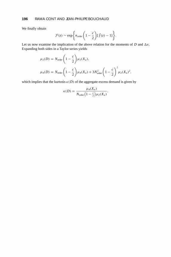
We finally obtain

F(z) ∼ exp

{norder

(1− c

2

)[ f (z)− 1]

}.

Let us now examine the implication of the above relation for the moments ofD and1x.Expanding both sides in a Taylor series yields

µ2(D) = Norder

(1− c

2

)µ2(Xα),

µ4(D) = Norder

(1− c

2

)µ4(Xα)+ 3N2

order

(1− c

2

)2

µ2(Xα)2,

which implies that the kurtosisκ(D) of the aggregate excess demand is given by

κ(D) = µ4(Xα)

Norder

(1− c

2

)µ2(Xα)

.

Documents

herd behavior and aggregate fluctuations in financial markets