Heliocentric Interplanetary Low-thrust Trajectory

The 31st International Electric Propulsion Conference, University of Michigan, USA

September 20 – 24, 2009

1

Heliocentric Interplanetary Low-thrust Trajectory Optimization Program Capabilities and Comparison to

NASA’s Low-thrust Trajectory Tools

IEPC-2009-214

Presented at the 31st International Electric Propulsion Conference, University of Michigan • Ann Arbor, Michigan • USA

September 20 – 24, 2009

Jerry L. Horsewood1

SpaceFlightSolutions™, Bowie, Maryland, 20720, U.S.A.

and

John W. Dankanich2

Gray Research, Inc., Cleveland, Ohio, 44135, U.S.A.

Abstract: Features and capabilities of the recently developed Heliocentric Interplanetary Low-thrust Trajectory Optimization Program (HILTOP™) are described and current development activities slated for completion in CY2009 are identified. An understanding of the scope and utility of the product is aided with a comparison to other low-thrust trajectory optimization and design tools, such as NASA’s Low-thrust Trajectory Tool (LTTT) suite and other legacy software. Optimal solutions produced by HILTOP for several complex, multi-leg missions are compared to those produced by MALTO (Mission Analysis Low-thrust Optimization), a member of NASA’s LTTT suite, and are found to match well. A final section of the paper describes the detailed modeling of the NASA NSTAR and NEXT thrusters and how those detailed models impact the optimization process and performance results.

Nomenclature 𝑓𝑓 = thrust produced by a thruster, N 𝑔𝑔 = acceleration due to Earth’s gravity at the equator = 9.80665 m/sec2

𝐼𝐼𝑠𝑠𝑠𝑠 = specific impulse of a thruster, sec �̇�𝑚 = total propellant flow rate of a thruster, kg/s 𝑠𝑠 = total power input to a power processing unit, W 𝑟𝑟 = distance of spacecraft from the sun, AU Δv = magnitude of change in velocity, m/sec 𝜂𝜂 = combined efficiency of a power processing unit and a thruster

I. Introduction ILTOP is a low-thrust mission analysis and trajectory optimization program with a legacy that spans four decades. It is designed for the analysis of electric propulsion space exploration missions in a heliocentric, two-

body environment. As such, it is considered to be of medium fidelity with respect to the gravitational model, suitable

1 Sole Proprietor, [email protected]. 2 Systems Engineer, NASA’s In-Space Propulsion Program, [email protected].

™ HILTOP, MAnE, and SpaceFlightSolutions are trademarks of Jerry L. Horsewood

H

mailto:[email protected]�


September 20 – 24, 2009

2

for early-to-intermediate phases of a mission study. This level of software is also commonly used during a mission to perform what-if studies, to evaluate sensitivities, and possibly to re-optimize the trajectory as random events and non-nominal performance cause the trajectory to deviate from its originally planned path. A properly configured solution from HILTOP will usually serve as an excellent first guess that leads to convergence to a solution in a high fidelity trajectory simulation program. Historically, low-thrust mission and trajectory optimization has been a coveted domain, open only to those who have, through necessity or foresight, invested in the development of the tools required to solve the difficult problem. Once developed, whether funded privately or by NASA, access to the tools historically has been restricted by the developing organizations for competitive advantage. This practice has not served the space exploration community well as it has limited the participation and the development of expertise to those few with access to the tools. The result is a space community that is dependent upon too few experienced analysts and a continuing lack of access to advanced tools. Access to NASA’s LTTT suite of tools has recently been relaxed to permit wider availability. The rules of access currently in effect for each of the tools in the suite are explained in Section III below. Recognizing a need for change, a redesign and redevelopment of HILTOP was initiated in 2003. The objectives of this effort were several: • To develop a commercial grade (i.e., robust, user-friendly, documented, continuously maintained, and responsive

to user needs and feedback) that is commercially available, along with training, to anyone; • To implement an object oriented design methodology that facilitates maintenance and future enhancements; • To employ modernized software development languages (Fortran 95, C#, and SQL); • To implement a variety of propulsion and power systems models that more accurately and robustly reflect the

operational characteristics of modern thrusters, including NASA’s NSTAR and NEXT technologies; and • To embed the trajectory optimization module, along with numerous supporting tools frequently used in low-

thrust mission analysis, within a graphical user interface (GUI) umbrella. This effort is now largely complete, although the GUI remains under development and is yet to be released. Current experience with HILTOP includes the analyses of numerous missions to comets, asteroids, and planets by and for clients of SpaceFlightSolutions and for use in program documentation. A major milestone was recently reached with the submittal of a New Frontiers proposal for which the mission design and optimization of a complex asteroid rendezvous mission were performed with HILTOP.

II. HILTOP Features and Capabilities The functionality and scope of HILTOP are divided into several categories that are described in the following

subsections. This breakdown is provided to facilitate the comparison of HILTOP features with those of other low-thrust trajectory tools that are described in Section III. Full software documentation is available to licensees in the form of two manuals1, 2 – “Mathematical Model of HILTOP” and “HILTOP User Guide.”

A. Mission Design Missions are composed of one or more distinct heliocentric legs, the terminals of which are solar system objects whose position and velocity at any instant of time are defined by an ephemeris. An exception exists for the last leg of a mission where the final target may be a partially or fully specified heliocentric orbit. A leg may consist of any number of successive thrust and coast phases. Successive legs of a mission are linked at a solar system body in a manner that simulates rendezvous with a finite stopover period or a flyby with no stopover. If the encounter is a flyby of a massive body (i.e., a planetary swingby), gravitational effects of the body on the spacecraft path are considered in terms of an instantaneous rotation of the hyperbolic excess velocity. The angle of rotation (the bend angle) is a function of the mass of the planet, the excess speed, and the passage distance of the spacecraft from the center of the planet at the time of closest approach. The number of legs is presently limited to 10 but may be increased by recompiling. Currently, the forces acting on the spacecraft that are included in the equations of motion are the gravitational attraction of the sun and the thrust of the electric propulsion system. Implementation of solar pressure force acting on solar arrays is in process and is expected to be complete by the end of CY2009. Planetocentric motion of the spacecraft at the terminal of a leg is evaluated with a methodology known as zero sphere of influence patched conics. In essence, it involves equating the relative velocity of the spacecraft at a terminal (evaluated as the vector difference of the heliocentric velocities of the spacecraft and the terminal body) with the planetocentric hyperbolic excess velocity. Any offset of the hyperbolic asymptote from the center of the body that is required to satisfy passage distances or capture orbit insertion may be safely ignored because the offsets required are infinitesimal relative to the distances of interplanetary space.


September 20 – 24, 2009

3

An analytic method is provided to estimate the time and propellant required for low-thrust escape from the launch body of the mission and/or capture at the final target body. Use of this model is optional and, if invoked, will usually involve lengthy periods to spiral up to or down from escape conditions. As an alternative to the low-thrust escape, the initial spacecraft mass may be equated to the payload capability of a specified launch vehicle, which is a function of launch C3, a parameter that is the square of the launch excess speed. This option is referred to as the Launch Vehicle Dependent (LVD) mode. Still another option, the Launch Vehicle Independent, or LVI, mode allows one to specify the initial spacecraft mass and the launch C3 independently. This option allows one to determine optimum launch conditions for a given mission and to select an appropriate launch vehicle later. For arrival at the final target, an option is provided to specify a high-thrust rocket to insert the spacecraft into a specified capture orbit after optionally ejecting portions or all of the propulsion and power systems.

B. Power Model The power model implemented in HILTOP is capable of supporting either nuclear or solar electric. The

difference between the two is that, in the absence of power decay or degradation, nuclear power is constant during the mission whereas solar power varies with spacecraft distance from the sun. Two formulations, one that originated in early versions of HILTOP and one that is used in most of the low-thrust tools developed at the Jet Propulsion Laboratory (JPL), are provided for representing solar array power as a function of solar distance, r. Both formulations require five coefficients to define the performance of a given array and both permit the inclusion of low intensity, low temperature (LILT) effects. Support is provided to maintain a file of coefficients representing numerous arrays, from which any one may be selected for the analysis of a mission.

Power decay/degradation may be applied to either the solar or nuclear electric power models. In either case it is specified as an initial decay amount, expressed as a percentage of array reference power, and a variable decay factor that is entered in units of %/year and may be applied as a linear or an exponential decay rate.

Once the power delivered by the power source is known, any amount specified for housekeeping purposes is satisfied first. The remaining available power is divided equally among the currently operating thrusters. If the power available to each thruster exceeds the maximum permissible input power (or the optimum input power if less than the maximum) to a power processing unit (PPU), the solar arrays are articulated to prevent the over production of power and the build-up of heat. If the power available to each thruster is less than or equal to the maximum usable power, the arrays are maintained at a normal orientation to the sun line, thereby producing the maximum power possible.

C. Propulsion System Model A primary objective of the redesign of HILTOP was to improve propulsion system modeling options to include

more detailed models of NASA’s NSTAR and NEXT thruster technologies as well as models consistent with other low-thrust trajectory tools to permit direct comparison of solutions. Three models are implemented, as follows: Classic Model – this model is consistent with those employed in most low-thrust trajectory tools prior to the mid-1990’s and continues to be used in early stage analyses where it is premature to consider the specifics of individual thrusters. It treats the specific impulse and the propulsion system efficiency as constants over the duration of the mission and accommodates variations in available power by varying the thrust. It maintains no recognition of individual thrusters; rather it treats the entire propulsion system as a single entity. This was the model implemented in the original HILTOP as well as in the program VARITOP developed and used at JPL from the early 1970’s to the mid-1990’s. Smooth Model – this model is predominant in current low-thrust mission analysis tools, including the entire spectrum of NASA’s LTTT software suite. The model is defined by polynomial expressions for thrust and propellant flow rate as a function of input power to the PPU. Normally, the polynomials are evaluated by performing least-squares curve fits of tabular data. In HILTOP, cubic splines are employed to yield functions that return exactly the tabular values and are continuous in the value of the function as well as its first and second derivatives over the entire power range. Once the thrust, f, and mass flow rate, m (a negative number), are known for a given PPU input power, p, the specific impulse, Isp, and propulsion system efficiency, η, at that operating point can be inferred with the equations:

)2/(

)/(2 pmf

mgfI sp

−=

−=

η (1)

where g = 9.80665 m/s2 is the acceleration due to gravity at the surface of the Earth.


September 20 – 24, 2009

4

Stepped Model – this model is unique to HILTOP, although variations of the concept have been implemented in the JPL/LTTT tools, Mystic and NEWSEP (see Section III). Its purpose is to more accurately represent the performance characteristics of NASA’s NSTAR and NEXT technologies. The model also directly supports Boeing’s 2-setting XIPS thruster. Other devices, such as the Hall thruster, are supported with the Smooth model. The operating points of supported thrusters are defined in subsets, called throttle levels, each spanning a portion of the total operating power range of the thruster. Within a throttle level, the propellant flow rate is constant and the thrust increases with increasing power. Specific impulse and propulsion system efficiency for this model are governed by Eq. 1 in the same manner as for the Smooth Model. Although operation of a thruster is limited to the discrete operating points that are defined, thrust, in the Stepped Model of HILTOP, is considered to be continuously variable over the range of power associated with a throttle level. Of course, the thrust and mass flow rate are discontinuous when the solution switches between throttle levels. An important distinction between the operating characteristics of the NSTAR and NEXT thrusters is that the power ranges for successive throttle levels overlap for the NEXT thruster but do not overlap for the NSTAR thruster. A consequence of this is that the Smooth and Stepped models yield much the same results for a mission that uses the NSTAR thruster because there is no choice as to which throttle level is used at a given power value. Conversely for the NEXT thruster with the Stepped Model, a decision is required at every point along the path as to which of the available throttle levels is currently optimum for the existing power level. In some cases, the result will favor higher thrust at the expense of specific impulse; in other cases the reverse will be true. Tabular data representing the performance of NEXT, taken from the most recent data published by NASA Glenn Research Center (GRC), is included in HILTOP and provisions exist to modify or update the tables by the user.

D. Ephemerides HILTOP includes an interface to the JPL planetary ephemeris file DE405 and a file that spans the entire twenty-

first century is provided as part of the program. Additionally, an interface to the JPL maintained file named Dastcom3 is provided. This file currently contains the orbital elements of over 460,000 asteroids and comets, each evaluated at a specific epoch. A recent copy of this file is also provided with HILTOP. These are standard files that are downloaded from the JPL web site and may be replaced by the user as updated files are made available by JPL.

One additional form of ephemeris files used by HILTOP is the User Defined Body (UDB) database. It allows one to define the orbital elements of objects that may then be used as launch or target bodies in HILTOP missions. It is particularly useful for representing the ephemeris of a comet or asteroid at an epoch that differs significantly from that at which the elements in a current version of the Dastcom3 file are evaluated. Because the orbits of these bodies are perturbed by the gravitational influences of the planets, the accuracy of position and velocity calculated with the orbital elements diminishes as the interval between the epochs of element evaluation and state evaluation increase. Clearly, propulsion requirements evaluated with inaccurate orbital elements of the target bodies will be correspondingly inaccurate. Updated values of comet and asteroid orbital elements may be obtained for any epoch from the Horizons web site that is maintained at JPL and included in a UDB data file. Software features within HILTOP are provided to create and maintain any number of UDB databases and also to facilitate the retrieval of data from the Horizons web site. The custom binary format of UDB files is common to HILTOP and to the high-thrust mission analysis tool, MAnE™, which is also developed and maintained by SpaceFlightSolutions.

E. Optimization Methodology HILTOP employs the indirect method of optimization commonly referred to as the Calculus of Variations

(CoV). This method involves the simultaneous solution of a set of differential equations that describe the behavior over time of the state variables of a problem as well as an equal number of adjoint, or co-state, variables. Solution by indirect methods eventually evolve into solving a multi-point boundary value problem (BVP) that entails the search for a set of unknown boundary values of state and co-state variables (i.e., the independent parameters of the problem) that result in the satisfaction of an equal number of constraint equations and equations of optimality, known as transversality conditions (collectively, the end conditions). The difficulty of solving the BVP causes some mission analysts to favor direct methods of optimization even though direct methods also require the solution of a BVP. The differences, however, are real and several: • The independent parameters of a CoV formulation include boundary values of the co-state variables whose

function and behavior are more obscure than their physical counterparts, the state variables. Thus, the task of estimating reasonable values to start the iterative search for the solution of the BVP is heuristic and one’s ability to successfully do this improves with experience. In the meantime, success appears to be more a result of art than of science.


September 20 – 24, 2009

5

• Instantaneous values of control variables of a CoV formulated problem are evaluated from current values of state and co-state variables; thus, once initial values of all state and co-state variables are specified, the trajectory plays out in the form of the integrated solution to the differential equations. There is no other way to influence the control variables or the path of the spacecraft.

• For direct optimization formulations, control variables are typically discretized input parameters that become independent parameters of the BVP. Although this substantially increases the order of the BVP compared to indirect methods, the influence of the independent parameters on the path of the trajectory are spread among the many parameters acting all along the path rather than the few acting just at the start of the mission. The consequence is that the proximity of the initial estimates of the independent parameters to their converged values need not be as close to achieve convergence to a solution with direct methods as with indirect methods.

• Adding constraints to a problem formulated with direct methods is rather simple – the equation of the constraint is defined and added as an end condition in the BVP. For problems formulated with indirect methods, it is also necessary to define the effect of the constraint on the remaining transversality conditions. In many CoV implementations, separate expressions for transversality conditions are developed for several combinations of imposed constraints, but this approach limits the program to those specific combinations that were considered. HILTOP circumvents this problem by implementing a process that automatically reconfigures transversality conditions for any combination of supported constraints.

• Indirect methods seek a solution that satisfies all constraints and achieves stationary conditions (i.e., zero slopes) of all degrees of freedom with respect to the independent parameters on which they depend. Advantages of this are that the convergence progress proceeds quadratically as the solution is neared (i.e., the number of significant digits of the final solution doubles each iteration) and the thrust/coast sequence is an output of the solution. On the other hand, indirect methods may converge to a solution that either maximizes or minimizes the optimization criterion with respect to an independent parameter and care must be exercised to assure that an obtained solution exhibits the desired characteristic.

• Direct methods seek a solution that satisfies all constraints while improving the value of the optimization criterion each iteration. The methods have the advantage of more quickly arriving in the vicinity of the optimum, but they lack knowledge of what explicitly represents the optimum solution. The result is that, contrary to the indirect methods, the iteration slows down as the iteration nears the solution and must eventually be terminated simply because of lack of progress. The direct methods also require input of the thrust/coast sequence of the solution, which may or may not be optimum.

Clearly, all optimization methodologies have advantages and disadvantages. In HILTOP, the choice of the indirect method reflects the belief that, with proper tools in place, the solution to electric propulsion missions of interest in the problem domain supported by HILTOP (i.e., heliocentric, two-body motion) are tractable with CoV for both simple and complex missions. Major effort has been devoted in the development of HILTOP to address usability issues, to provide a robust and powerful iterator to solve the BVP, to develop numerous aids that assist the analyst in performing his/her functions, and to document well over a dozen examples of how to approach a complex problem for analysis and solution. The additional missions described in the following paragraphs further demonstrate that indirect methods can be very effective in addressing some of the more complex solar system exploration missions under current consideration.

F. Mission Model Refinements It is customary in early-stage mission design and optimization to ignore certain details or desired characteristics

of a mission, or to represent them with simplified models, because to do otherwise is considered to be too difficult or too expensive for the benefit and additional accuracy achieved. Accepted practice is to design the mission with the simplified models while imposing substantial contingencies and margins on performance requirements that will cover the uncertainties introduced by the models. This is an entirely reasonable and responsible approach given the sheer volume of cases that are typically needed to eventually arrive at a mission design that best meets overall mission objectives. However, at some point in the analysis it is prudent to begin to assess these issues in greater detail to avoid surprises that may otherwise occur late in the design process when they become much more expensive to resolve.

Several features have been incorporated in HILTOP that allow one to assess the effects of influences that are not normally considered in early stage analyses. Probably the most notable among these is the Stepped propulsion model. This model was used exclusively in the analysis of the proposed New Frontiers asteroid rendezvous mission, but more likely will be used by others as a final adjustment to a mission design performed with either the Smooth or


September 20 – 24, 2009

6

the Classic model. Besides adding accuracy to the results, it provides useful information on the operational control of the thrusters over the course of the mission. Other features offering added detail are as follows: Imposed coast phase schedule – It is common practice to model unplanned propulsion system downtime with a concept known as duty cycling. The objective in mission design is to assure a sufficiently robust solution such that, if the propulsion system had to be shut down for some period of time, the mission is still achievable. The concept of duty cycling equates a percentage reduction in the rated output power of the power source to an equivalent percentage of thruster downtime. While this is fairly accurate for some missions, it is not for others so it is important to check this by introducing forced downtime in the trajectory simulation. HILTOP achieves this by allowing one to specify a schedule of times and durations that the engines are shut down and optimize the trajectory subject to this schedule. RCS propellant depletion schedule – Propellant consumption by the reaction control system is not deterministic. Nevertheless, the fact that RCS propellant will be needed throughout the mission is unquestioned. This feature allows one to factor into the analysis a schedule of RCS propellant depletion events to add realism to the solution and to assess the effect on the low-thrust propulsion requirements. The sole effect of the event on the state of the spacecraft is the reduction of mass. The amount of propellant expended at each event may be specified either as a constant mass drop or as a Δv from which the mass drop is calculated. Control schedule for number of operating thrusters – The CoV optimization process returns the optimum number of thrusters, subject to an input maximum and minimum, that should be operating at any point along the trajectory. Occasionally this process will lead to results that are operationally undesirable. To override the result, the ability to temporarily change the upper and lower limits on the number of operating thrusters is provided.

G. Constraints and End Conditions Much of the usefulness of a mission optimization program is tied to the range of constraints that are available for

specification to define a mission. The absence of a constraint on a specific parameter implies that the parameter is optimized as a consequence of satisfying all transversality conditions and the constraints that are in effect. In addition to the constraints on position and, if applicable, the velocity of the spacecraft at departure and arrival of each leg, the principal constraints provided in HILTOP include the following: • Departure and arrival dates for each leg; • Flight times of individual legs and/or of the entire mission; • Stay times between legs of stopover missions; • Departure and arrival excess speeds for each leg; • Arrival velocity vector relative to the target body (for rendezvous or capture missions); • Launch asymptote declination; • Final spacecraft mass, net payload, or propellant mass; • Any combination of the orbital elements of a final heliocentric orbit; • Reference power; • Jet exhaust speed (Classic propulsion model only); • Cumulative operating time of individual thrusters over a mission; • Passage distance at swingby events; • Total travel angle for a mission; and • Thrust angle relative to the sun line at solar distances below a threshold value. Once the applicable constraints for a mission are defined, the applicable transversality conditions that are most likely to apply are automatically identified and invoked without user specification. For example, if launch excess speed is not constrained, a corresponding transversality condition is invoked. There exist situations, however, where the most likely assignment of transversality conditions is not what is desired. For example, suppose one is generating a sequence of solutions for a discrete set of launch dates with the launch excess speed optimized for each case. In this situation, the launch date is constrained for each case (hence, no transversality condition) and the transversality condition for launch excess speed is invoked. Now, suppose that one is interested in the solution within this sequence for which the optimized launch excess speed is a specific value. But, if one were to simply constrain launch excess speed to the desired value and remove the constraint on launch date, the wrong transversality condition (i.e., the one associated with launch date) would be invoked. To resolve this situation while retaining the automatic selection of transversality conditions normally desired, the Boolean attributes of Ignore and Force, both of which are normally false, are provided for each transversality condition. The proper settings of these attributes allow one to alter the manner in which an optimization problem is posed.


September 20 – 24, 2009

7

H. Reporting and Graphics The amount of data generated in a typical execution of HILTOP is quite large and the task of presenting that data

to the user in a useful way is challenging. If an execution fails to converge to a solution, the need is for information about the iteration process that is sufficiently detailed to permit identification of the problem(s) that may have prevented convergence. On the other hand, if an execution converged, interest will be on the data that describes that solution. In HILTOP, this problem is addressed by producing 20 distinct reports, some of which are optional and some are dependent on the modes and models specified for the mission being analyzed. The majority of the reports are written as tab-delimited text files that are intended to be opened in a spreadsheet program to permit easy viewing, data manipulation, and plotting. These reports are designed to meet the needs of different subsystem engineers that require information as a function of time in a variety of coordinate systems, such as ecliptic, Earth equatorial, or body fixed. Other reports are designed for the mission analyst and include summary information of multiple cases incorporated in a single execution. Certain optional specialty reports are also produced, such as a spacecraft ephemeris file in SPK format, a standard format that is employed in several tools used in the space exploration community.

In addition to the plotting capabilities inherent with spreadsheet programs using the tab-delimited HILTOP output files, an ecliptic plane projection of the trajectory profile can be plotted directly from HILTOP from a binary file, which is one of the 20 output files produced by HILTOP. Examples of the trajectory profile plots are provided below in the comparison of mission solutions produced by HILTOP and MALTO. The binary file may also be used as input to a feature within MAnE that evaluates close encounters of a spacecraft with all bodies, or some subset, whose ephemerides are provided within DE405, the Dastcome3 file, and a named UDB file.

I. Supporting Tools Several utility/support programs are provided with HILTOP to perform necessary tasks that create input data for

HILTOP and that produce additional reports that are occasionally needed. Currently, six such tools are provided, as follows: Solar array coefficients generator – given a table of solar array power output values as a function of solar distance, this program solves for the coefficients used by the program to evaluate power available to the spacecraft and propulsion system during a mission. One may optionally produce the coefficients for either the HILTOP or the JPL formulation of the power model. Launch vehicle coefficients generator – given a table of launch vehicle payload mass capability as a function of launch C3, this tool solves for the coefficients of the expression used to model launch vehicle performance. User-defined body ephemeris file – this program accepts as input a set of orbital elements, the gravitational constant, and the equatorial radius of a body and adds the information to a specified UDB database file. If the file does not previously exist, it is created before the data is added. Solar system body ephemeris report – this program creates a tab-delimited text file containing the ephemeris of any solar system body whose ephemeris can be retrieved or evaluated from the DE405, Dastcom3, or UDB data files. Position and velocity component values in both Cartesian and polar coordinates are listed for a defined calendar period and interval between points. Creation of spacecraft ephemeris file in SPK format – this program writes the ephemeris of a spacecraft trajectory to a binary file in the widely used SPK format. An option exists to write either a Type 9 or a Type 13 format file. Horizons interface tool – this program is designed to automate some of the tasks of requesting and processing updated asteroid and comet orbital elements from JPL’s Horizons system. The tool includes a template for requesting the elements of a specific body at a given epoch using the e-mail option of the Horizons system. The tool then accepts the response files of one or more requests and passes them through a filter that formats the appropriate data for input to the UDB maintenance tool for updating a named UDB file.

III. Description of LTTT Suite and Legacy Tools To help place the features and capabilities of HILTOP in context, a brief discussion of alternative tools presently

in use and of legacy software is provided. Specifically, four legacy software tools and four tools comprising the LTTT software suite are discussed. The LTTT suite was developed at the direction of NASA’s In-Space Propulsion Technology (ISPT) Project to provide a set of low-thrust trajectory tools that are well documented, yield consistent results and have improved ease-of-use compared to previous tools. All of the tools in the suite use ephemeris files that are maintained by JPL. Descriptions of the LTTT suite and of the project are given in Ref. 3 and Ref. 4. Portions of the software descriptions provided below are taken from those documents.


September 20 – 24, 2009

8

A. Legacy Software Tools CHEBYTOP – Legacy low-thrust trajectory optimization tools in use at ISPT are CHEBYTOP, VARITOP, SEPTOP, and NEWSEP. CHEBYTOP is a tool originally developed at The Boeing Company in 1969. Numerous updates have been developed over the years by Boeing, JPL, and GRC. The NASA Marshall Spaceflight Center (MSFC) has developed also an Excel-based version for parametric assessment. CHEBYTOP uses Chebychev polynomials to represent state variables. These polynomials are then differentiated and integrated in closed form to solve for a variable thrust trajectory. CHEBYTOP is not capable of analyzing multi-leg missions such as round trip flights, intermediate flybys, or multi-body trajectories. CHEBYTOP is also limited to interplanetary missions with only the Sun’s gravity field. CHEBYTOP is considered a low-fidelity program by today’s standards, but has been highly valued and is openly and freely available without user restrictions. CHEBYTOP is considered appropriate for collegiate level analysis. VARITOP, SEPTOP, and NEWSEP – VARITOP is the Variational calculus Trajectory Optimization Program developed at JPL and SEPTOP and NEWSEP are updates/extensions to VARITOP for specific applications. VARITOP is a general tool that can analyze nuclear electric propulsion (NEP), solar electric propulsion (SEP), or solar sail trajectories. The three tools are all based on the same mathematical formulation and share many common subroutines. The calculus of variations is used in the formulation of state and co-state equations that are integrated numerically to solve a two-point boundary value problem. The mathematical formulation is quite similar to that of HILTOP as described above.

The Solar Electric Propulsion Trajectory Optimization Program (SEPTOP) is an extension of VARITOP that adds solar array fidelity, thruster throttling, and a variable number of operating thrusters. SEPTOP can use thrust and propellant flow rate polynomials to represent the performance of specific thrusters. SEPTOP also uses polynomials to represent solar array performance as a function of distance from the sun and may include low intensity low-temperature (LILT) effects. Provisions also exist to model power degradation over time. NEWSEP is a slight variation of SEPTOP that can use specific throttle points rather than polynomial curves to represent the thruster characteristics. These legacy tools were used to provide trajectory support for the Deep Space 1 mission and are considered medium fidelity. The legacy tools are no longer maintained and have limited availability, primarily for academic use only through JPL.

B. LTTT Software Suite MALTO – The Mission Analysis Low-Thrust Optimization tool was specifically developed as a more “user friendly” medium fidelity optimization tool with relatively easy convergence, especially for missions with multiple gravity assists. MALTO uses many impulsive burns to simulate a continuous burn trajectory about a single gravitational source. The mission setup, parametric trades, and post-processing can be performed with a MATLAB based graphical user interface (GUI). The thruster and power system modeling is comparable to the VARITOP based programs. Optimization in MALTO is calculated using the SNOPT code developed independently. MALTO is available freely to NASA contractors, civil service, and academia, and can be purchased commercially though the Caltech Office of Technology Transfer. The design of this tool is described in Ref. 5. Copernicus – Copernicus is a generalized trajectory design and optimization program that allows the user to model simple to complex missions using many objective functions, optimization variables and constraint options. Copernicus was originally developed by the University of Texas at Austin, but the development has since been transferred to the NASA Johnson Spaceflight Center (JSC). With Copernicus, one can model events ranging from simple impulsive maneuvers about a point mass to multiple spacecraft with multiple finite and impulse maneuvers in complex gravitational fields. The tool uses a graphical output for real time feedback during the optimization process. Copernicus is an n-body high fidelity tool. Copernicus is freely available, but with limited distribution to NASA and NASA contractors. OTIS – The Optimal Trajectories by Implicit Simulation program was developed by GRC and Boeing. Earlier versions of OTIS have primarily been launch vehicle trajectory analysis programs, but have since been updated for robust and accurate interplanetary mission analysis, including low-thrust trajectories. The tool is named for its original implicit integration method, but also includes explicit integration and analytic propagation. Vehicle models can be very sophisticated and can be simulated through six degrees of freedom. OTIS uses third party SLSQP and SNOPT to solve the nonlinear programming problem associated with the solution of the implicit integration method. OTIS is a high fidelity optimization and simulation program. OTIS source code is freely available to anybody in government, academia, and industry through the GRC technology transfer office, subject to export control regulations. Mystic – Mystic was developed at JPL. The tool uses a Static/Dynamic optimal control (SDC) method to perform nonlinear optimization. Mystic is an n-body tool and can analyze interplanetary missions as well as planet-centered


September 20 – 24, 2009

9

missions in complex gravity fields. Mystic can automatically find and use gravity assist options. Mystic also allows the user to plan for spacecraft operation and navigation activities. The mission input and post-processing can be performed using a MATLAB based GUI. Mystic is currently used on the Dawn mission, and is a considered a high fidelity optimization and simulation program. Mystic is currently available to NASA only and requires considerable tool specific expertise to operate successfully.

IV. Comparison of Mission Solutions by HILTOP and MALTO Four missions of varying complexity were identified for comparing results produced by HILTOP and MALTO.

The simplest of these is a Mars orbiter mission that employs low-thrust for the interplanetary transfer as well as for establishing the low orbit about Mars. The second mission is representative of the Dawn mission; however, the propulsion technology assumed is that of NEXT rather than the NSTAR technology actually used in the Dawn mission. The Dawn mission includes a Mars swingby, followed by a second leg terminating with rendezvous and stopover at Vesta, and a third leg ending with rendezvous at Ceres. The third mission is known as Near Earth Asteroid Return Earth Return, or NEARER, which is, in essence, a double asteroid sample return mission. It begins with a low-thrust transfer, rendezvous, and stopover at the first asteroid where a sample is retrieved. The mission continues with a low-thrust transfer to Earth swingby where the sample is ejected for atmospheric entry. The third leg of the mission follows Earth swingby with a low-thrust transfer to the second asteroid where the sample retrieval process is repeated. A final leg then follows with a low-thrust transfer back to Earth where the sample is ejected for aerodynamic entry. The final, and most complex, mission compared is the Titan Saturn System Mission (TSSM) that employs low-thrust assisted by four planetary swingbys, one of Venus and three of Earth, in the sequence E-V-E-E.

For comparison purposes, a simple (1/r2) power law was assumed for solar array performance. The Smooth propulsion system model was specified for all HILTOP cases because it corresponds to the only model supported by MALTO. Linear relationships of the thrust and mass flow rate as a function of PPU input power over the operating range of NEXT were specified for both programs, as shown in Table 1. The use of linear performance parameter relationships removes any differences that might exist between the polynomial representation used in MALTO and the cubic spline representation used in HILTOP, as both exactly model straight lines.

Each of the four missions has been previously studied by NASA, so known solutions existed at the start of this comparison study. Both HILTOP and MALTO require that one specify the sequence of targets to be included in a mission and the information from the prior studies were used for this purpose. No other sequences were considered. Knowledge of the details from existing solutions can be used to advantage by both HILTOP and MALTO in arriving at a converged trajectory, although the advantage gained is probably greater for HILTOP. Of course, neither program requires such detailed knowledge. The following subsections describe the results of the study.

A. Mars Orbiter Mission The specifications for this mission are given in

Table 2. This mission requires a relatively high array power in order to accomplish the spiral capture maneuver by the specified date. Note that the power is sufficient to operate both thrusters at maximum power at 1 AU and below. The limit on launch declination is consistent with a launch from the Guiana Space Center located near Kourou, French Guiana.

Data representing the continuous thrust solutions produced by MALTO and HILTOP are shown in Table 3. The solutions use both thrusters for the entire mission even though the power produced by the array at Mars is less than the maximum power usable by one thruster. This is optimal because the mission benefits from higher acceleration, which is achieved with two thrusters operating rather than one. It is interesting to note that the payload capability of the Atlas V 531 for the launch C3 values shown in the table exceeds 2,800 kg. Clearly, it possesses excess capacity for this mission, a fact that was identified by both programs. Allowing greater initial mass than that shown in Table 3 results in a smaller final mass, making such a solution less optimum.

Table 1. NEXT Performance Limits

Power (W) Thrust (mN) Flow Rate (mg/s) Min Value 600 27.0226 1.4854 Max Value 7,100 240.8791 6.0289

Table 2. Mars Orbiter Mission Specifications

Array power at 1 AU 15 kW Duty cycle 100%

Housekeeping power 0.25 kW Thrusters 2 NEXT

Launch vehicle Atlas V 531, no contingency Launch declination limits ± 6°

Launch date Anytime in 2022 Arrival date in final orbit Not later than May 15, 2024

Final orbit at Mars 500 km altitude circular


September 20 – 24, 2009

10

The differences in the solutions of the two programs are small, but noticeable. HILTOP predicts shorter flight times (0.5% for the cruise phase and 2% for the capture phase) and optimizes to a higher initial spacecraft mass (3.9%). The cruise propellant predicted by HILTOP is also larger in proportion to the larger initial mass, but the capture propellant estimate predicted by HILTOP is larger by 20.5% than that of MALTO. This latter difference is attributed to the different analytic models employed in the two programs that estimate the low-thrust capture time and propellant. Together, these factors lead to the 2.5% higher final mass of the HILTOP solution.

The ecliptic plane projection of the trajectory profile of the mission is shown in Fig. 1. The creation of these drawings is a feature of HILTOP. In these drawings, planetary orbits are drawn in blue, comet and asteroid orbits in cyan, and the spacecraft trajectory in red with thrusting portions of the trajectory shown in a bolder red. Red dots mark the locations of launch and target bodies at the time of encounters and red tick marks along the path denote the division between thrust and coast periods. In this case the propulsion system operates continuously for the entire mission. When thrusting, the direction of the thrust vector is shown by grey vectors emanating from the path. The bold grey vectors at the mission launch and target bodies denote the hyperbolic excess velocity vector at the time of encounter. For swingby events, two vectors denoting the arriving and departing excess velocities are shown. The absence of such a vector at a target body means that the hyperbolic excess speed is zero at that point. The green background of horizontal and vertical axes with hash marks, and of several concentric dashed circles, aid in the visual perception of the orbits and the trajectory. The scale of the drawing may be selected such that any portion or the entire mission can be displayed with the desired resolution. Annotations can be created and located on the drawing as desired.

Several variables that are normally of interest to mission analysts are shown in Fig. 2 as a function of time along the trajectory. Graphs such as this may be created within Excel using tab-delimited files that are output by HILTOP for the converged solution. Along the left vertical axis, the graph shows the values of the power available to the operating thrusters, the power used by those thrusters, the distance of the spacecraft from the sun and the Earth, and a variable that is ten times the thrust level. The value of specific impulse is shown along the right vertical axis.

Table 3. Mars Orbit Mission Solution Comparison

Parameter MALTO HILTOP Launch date 3/29/2022 4/7/2022 Launch C3 (km2/s2) 32.26 32.57 Launch declination (deg) -5.1 -3.776 Launch mass (kg) 2,105.4 2,187.3 Cruise flight time (days) 458.2 455.7 Cruise propellant (kg) 324.3 338.7 Mars Arrival date 7/1/2023 7/6/2023 Spiral capture time (days) 319.9 313.73 Capture propellant (kg) 129.7 156.30 Final orbit arrival date 5/15/2024 5/15/2024 Final mass (kg) 1,651.4 1,692.3

Figure 1. Mars Orbiter Mission Trajectory Profile


September 20 – 24, 2009

11

B. Dawn Mission The specifications for this mission are given in

Table 4. This mission approximates the Dawn mission that is currently en route to Vesta, having passed Mars in February of 2009. The principal difference is that this mission specifies the NEXT thruster whereas the Dawn mission actually uses a series of three NSTAR thrusters operating one at a time. A thruster startup delay of 45 days is specified to provide time for array deployment and propulsion system checkout. The Earth launch and Mars swingby dates are fixed for this study at the dates of occurrence in the actual mission. The specification of date ranges for arrival at the two asteroids reflects the fact that the spacecraft has sufficient margins to successfully accomplish the mission even if significant interruptions in thruster operation occur. Should this happen, the arrival date(s) can be adjusted as necessary to accomplish the approaching rendezvous. For this study, the objective is to optimize the arrival dates within the specified ranges, subject to all the other constraints of the mission. The limit on launch declination is consistent with a launch from the Eastern Test Range at Cape Canaveral, Florida.

A summary of the optimal solutions produced by MALTO and HILTOP for the Dawn mission is given in Table 5. Generally speaking, the results of the two programs match quite well, as is evident from the graph of thrust as a

Table 4. Dawn Mission Specifications

Array power at 1 AU 10.3 kW Duty cycle 100%


Launch vehicle Delta II 2925-9.5, no contingency

Launch declination limits ± 28.5° Thruster startup delay 45 days

Launch date 9/27/2007 Mars swingby date 2/17/2009

Minimum passage altitude 300 km Arrive at Vesta Anytime in August 2011

Stay time at Vesta 270 days Arrive at Ceres Anytime in February 2015

Figure 3. Comparison of Thrust Magnitudes for Dawn Mission

0

0.05

0.1

0.15

0.2

0.25

0.3

0 500 1000 1500 2000 2500 3000

Thru

st (N

)

Time from Launch (days)

HILTOPMALTO

Mars Swingby Depart Vesta

Arrive Vesta Arrive Ceres

Figure 2. Variable Time Histories for the Mars Orbiter Mission

2500

2700

2900

3100

3300

3500

3700

3900

4100

4300

4500

0

2

4

6

8

10

12

14

16

18

20

0 50 100 150 200 250 300 350 400 450 500

Spec

ific

Impu

lse

(sec

)

Pow

er (k

W),

Dis

tanc

e (A

U),

Thru

st (N

) x 1

0


Power Available

Power Used

Solar DistEarth Dist


September 20 – 24, 2009

12

function of time from launch in Fig. 3. The variations in values of mass parameters shown in Table 5 stem from the difference in values of launch mass. This is attributed to minor differences in the manner in which launch vehicle payload as a function of C3 is modeled in the two programs. The Earth departure and Mars arrival dates are fixed for this mission, so these dates match identically. The dates of arrival at Vesta and Ceres are specified to be within a range covering one calendar month each, and both programs optimize to a bound of these ranges – the opening of the range for arrival at Vesta and the closing of the range at Ceres. However, the Mars-Vesta leg ends with a coast phase that starts 66 days prior to the designated Vesta arrival date. Thus, the rendezvous necessarily occurred 66 days earlier than specified; i.e., when the coast period started. This result was obtained by both programs.

The launch declination for an unconstrained solution exceeds the specified limit by about 1 degree. Therefore, the constraint has a minor effect on the solution in this case.

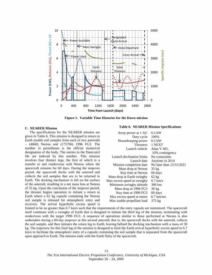
The ecliptic plane projection of the Dawn trajectory profile produced by HILTOP is shown in Fig. 4 and a graph of selected variables of interest are presented as a function of time from launch in Fig. 5. The vertical black dotted lines represent the times of encounter of the spacecraft with the several targets. Gaps in the propulsion system parameters Thrust and Specific Impulse appear during coast phases.

Table 5. Dawn Mission Solution Comparison

Parameter MALTO HILTOP Leg 1 Earth-Mars Launch date 9/27/2007 9/27/2007 Launch C3 (km2/s2) 5.1529 5.2285 Launch declination (deg) 28.5 28.5 Launch mass (kg) 1,114.4 1,105.2 Flight time (days) 510 510 Arrival mass (kg) 1,039.8 1,032.7 Propellant used (kg) 74.6 72.4 Leg 2 Mars-Vesta Swingby date 2/18/2009 2/18/2009 Swingby v∞ (km/s) 4.10 4.11 Passage altitude (km) 300 300 Flight time (days) 894 827.7 Arrival date 8/1/2011 5/26/2011 Arrival mass (kg) 907.3 901.4 Propellant used (kg) 132.5 131.3 Stay time (days) 270 336.3 Leg 3 Vesta-Ceres Departure date 4/27/2012 4/27/2012 Flight time (days) 1,038 1,038 Arrival date 2/28/2015 2/28/2015 Arrival mass (kg) 807.2 802.3 Propellant used (kg) 100.1 99.1 Total Propellant (kg) 307.2 302.8 Mission duration (days) 2,711 2,711

Figure 4. Dawn Trajectory Profile


September 20 – 24, 2009

13

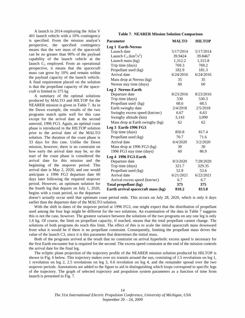
C. NEARER Mission The specifications for the NEARER mission are

given in Table 6. This mission is designed to return to Earth sizable soil samples from each of two asteroids – (4660) Nereus and (175706) 1996 FG3. The number in parentheses is the official numerical designation of the body. The entries in the Dastcom3 file are indexed by this number. This mission involves four distinct legs, the first of which is a transfer to and rendezvous with Nereus where the spacecraft remains for 60 days. During the stopover period, the spacecraft docks with the asteroid and collects the soil samples that are to be returned to Earth. The docking mechanism is left on the surface of the asteroid, resulting in a net mass loss at Nereus of 35 kg. Upon the conclusion of the stopover period, the thruster begins operation to initiate a return to Earth where a 62 kg capsule containing the Nereus soil sample is released for atmospheric entry and recovery. The arrival hyperbolic excess speed is limited to be no greater than 6.7 km/s such that the requirements of the entry capsule are minimized. The spacecraft itself continues with a swingby of Earth that is designed to initiate the third leg of the mission, terminating with rendezvous with the target 1996 FG3. A sequence of operations similar to those performed at Nereus is also undertaken during a 60-day stopover at this second asteroid; that is, the spacecraft docks with the asteroid, collects the soil sample, and then initiates the return leg to Earth, leaving behind the docking mechanism with a mass of 30 kg. The trajectory for this final leg of the mission is designed to limit the Earth arrival hyperbolic excess speed to 6.7 km/s to facilitate the atmospheric entry of a capsule containing the soil sample that is separated from the spacecraft upon approach to Earth. The mission ends with the Earth flyby of the spacecraft.

Figure 5. Variable Time Histories for the Dawn mission

0

1000

2000

3000

4000

5000

0

2

4

6

8

10

0 400 800 1200 1600 2000 2400 2800

Spec

ific

Impu

lse

(sec

)

Pow

er (k

W),

Dis

tanc

e (A

U),

Thru

st (N

) x 1

0


EarthDistance

SolarDistance

Power Available

Power Used

Mars Swingby

Designated Vesta Arrival

Vesta Departure

Ceres Arrival

Table 6. NEARER Mission Specifications

Array power at 1 AU 6.5 kW Duty cycle 100%


Launch vehicle Atlas V 401, 10% contingency

Launch declination limits No constraints Launch date Anytime in 2014

Mission completion date No later than 12/31/2021 Mass drop at Nereus 35 kg Stay time at Nereus 60 days

Mass drop at Earth swingby 62 kg Max excess speed at swingby 6.7 km/s

Minimum swingby altitude 300 km Mass drop at 1996 FG3 30 kg Stay time at 1996 FG3 60 days

Max excess speed at return 6.7 km/sec Max usable propellant load 375 kg


September 20 – 24, 2009

14

A launch in 2014 employing the Atlas V 401 launch vehicle with a 10% contingency is specified. From the mission analyst’s perspective, the specified contingency means that the wet mass of the spacecraft can be no greater than 90% of the payload capability of the launch vehicle at the launch C3 employed. From an operational perspective, it means that the spacecraft mass can grow by 10% and remain within the payload capacity of the launch vehicle. A final requirement placed on the solution is that the propellant capacity of the space-craft is limited to 375 kg

A summary of the optimal solutions produced by MALTO and HILTOP for the NEARER mission is given in Table 7. As in the Dawn example, the results of the two programs match quite well for this case except for the arrival date at the second asteroid, 1996 FG3. Again, an optimal coast phase is introduced in the HILTOP solution prior to the arrival date of the MALTO solution. The duration of the coast phase is 33 days for this case. Unlike the Dawn mission, however, there is no constraint on how early the arrival date may be, so the start of the coast phase is considered the arrival date for this mission and the beginning of the stopover period. This arrival date is May 2, 2020, and one would anticipate a 1996 FG3 departure date 60 days later following the required stopover period. However, an optimum solution for the fourth leg that departs on July 1, 2020, begins with a coast period, so the departure doesn’t actually occur until that optimum coast period ends. This occurs on July 28, 2020, which is only 6 days earlier than the departure date of the MALTO solution.

With the shift in dates of the stopover period at 1996 FG3, one might expect that the distribution of propellant used among the four legs might be different for the two solutions. An examination of the data in Table 7 suggests this is not the case, however. The greatest variance between the solutions of the two programs on any one leg is only 1.6 kg. Of course, the limit on propellant capacity, if reached, means that the total propellant cannot change. The solutions of both programs do reach this limit. The effect of this is to scale the initial spacecraft mass downward from what it would be if there is no propellant constraint. Consequently, limiting the propellant mass drives the value of the launch C3, since it is this parameter that determines the initial mass.

Both of the programs arrived at the result that no constraint on arrival hyperbolic excess speed is necessary for the first Earth encounter but is required for the second. The excess speed constraint at the end of the mission controls the arrival date for the final leg.

The ecliptic plane projection of the trajectory profile of the NEARER mission solution produced by HILTOP is shown in Fig. 6 below. This trajectory makes over six transits around the sun, consisting of 1.5 revolutions on leg 1, 1 revolution on leg 2, 2.5 revolutions on leg 3, 0.6 revolution on leg 4, and the remainder spread over the two stopover periods. Annotations are added to the figure to aid in distinguishing which loops correspond to specific legs of the trajectory. The graph of selected trajectory and propulsion system parameters as a function of time from launch is presented in Fig. 7.

Table 7. NEARER Mission Solution Comparison

Parameter MALTO HILTOP Leg 1 Earth-Nereus Launch date 5/17/2014 5/17/2014 Launch C3 (km2/s2) 39.9424 39.8467 Launch mass (kg) 1,312.2 1,315.8 Trip time (days) 769.3 769.2 Propellant used (kg) 182.9 181.3 Arrival date 6/24/2016 6/24/2016 Mass drop at Nereus (kg) 35 35 Nereus stay time (days) 60 60 Leg 2 Nereus-Earth Departure date 8/23/2016 8/23/2016 Trip time (days) 530 530.3 Propellant used (kg) 68.6 68.5 Earth swingby date 2/4/2018 2/5/2018 Swingby excess speed (km/sec) 6.67 6.63 Swingby altitude (km) 3,143 3,090 Mass drop at Earth swingby (kg) 62 62 Leg 3 Earth-1996 FG3 Trip time (days) 850.8 817.4 Propellant used (kg) 70.7 71.6 Arrival date 6/4/2020 5/2/2020 Mass drop at 1996 FG3 (kg) 30 30 1996 FG3 stay time (days) 60 86.9 Leg 4 1996 FG3-Earth Departure date 8/3/2020 7/28/2020 Trip time (days) 321.7 329.35 Propellant used (kg) 52.8 53.6 Arrival date 6/21/2021 6/22/2021 Arrival excess speed (km/sec) 6.7 6.7 Total propellant (kg) 375 375 Earth arrival spacecraft mass (kg) 810.2 813.8


September 20 – 24, 2009

15

Figure 6. NEARER Trajectory Profile

Figure 7. Variable Time Histories for the NEARER mission

0

500

1000

1500

2000

2500

3000

3500

4000

4500

0

2

4

6

8

10

0 300 600 900 1200 1500 1800 2100 2400 2700

Spec

ific

Impu

lse

(sec

)

Pow

er (k

W),

Dis

tanc

e (A

U),

Thru

st (N

) x 1

0


Nereus Stopover

1996 FG3 Stopover

Nereus Stopover

1996 FG3 Stopover

Power Available

Power Used

Earth Dist

Solar Dist

Earth Swingby

Earth Return


September 20 – 24, 2009

16

D. Titan Saturn System Mission (TSSM) TSSM was one of two missions proposed

for the joint NASA/ESA Outer Planet Flagship Mission (OPFM) project. Although it was not selected for the mission to be launched in the 2020 time period, it remains under considera-tion for a later launch opportunity. A low-thrust option was considered for the mission, and the trajectory analyzed in this example is developed with the swingby target sequence and target dates of the proposed low-thrust trajectory in mind. Several important aspects considered in the TSSM proposal are ignored in this analysis, so the solutions arrived at here differ somewhat from that proposed. The specifications for this version of the TSSM mission are given in Table 8. The mission employs the Atlas V 551 launch vehicle and two NEXT thrusters powered by a 15 kW array to deliver maximum mass to Saturn about 9 years after launch. The flight path makes four full revolutions about the sun and includes three swingbys of Earth and one of Venus. Objectives of this example are to optimize the launch date within the range specified in the table and to optimize all the swingby dates. The Saturn arrival date is constrained to limit the mission duration.

A comparison of results of the MALTO and HILTOP solutions is shown in Table 9. Here one sees that the solutions are nearly identical for the first three legs of the mission. Minor differences in the propellant expended occur on Leg 4 (MALTO requires 7.5 kg more than HILTOP), but the situation reverses on the last leg, leading to an insignificant difference of only 0.6% at the end of the mission. Even more remarkable is the fact that the final spacecraft mass of the two solutions differs only by 0.01% (0.75 kg). The ecliptic plane profile of the TSSM trajectory is shown in Fig. 8. The scale of this figure is chosen to better display the portions of the mission where the propulsion system is operating. The portion of the final leg that is not shown is a coasting arc that terminates at Saturn arrival. One will note that there are three thrusting arcs on Leg 1 of the mission, two on Leg 4, and one at the start of Leg 5. Legs 2 and 3 are coasting arcs in their entirety. A graph showing the time histories of several variables of interest for the mission are shown in Fig. 9.

Table 8. TSSM Specifications

Array power at 1 AU 15 kW Duty cycle 100%

Housekeeping power 0 kW Thrusters 2 NEXT

Launch vehicle Atlas V 551, no contingency

Launch declination limits 28.5˚ Launch date September 10 – 30, 2020

First Earth swingby date ~ October 27, 2021 Venus swingby date ~ February 4, 2022

Second Earth swingby date ~ June 11, 2023 Third Earth swingby date ~ June 11, 2025

Saturn arrival date October 28, 2029


September 20 – 24, 2009

17

Table 9. TSSM Solution Comparison

MALTO HILTOP Leg 1 Earth-Earth Departure date 9/10/2020 9/10/2020 Launch C3 (km2/s2) .5329 0.5392 Launch declination (deg) -19.9 -19.9 Launch mass (kg) 6,271.8 6,270.21 Flight time (days) 412 411.2 Arrival mass (kg) 6,058.0 6,058.18 Propellant used (kg) 213.8 212.03 Leg 2 Earth-Venus Swingby date 10/27/2021 10/26/2021 Swingby v∞ (km/s) 3.65 3.63 Passage altitude (km) 15,527 15,705 Flight time (days) 101. 102.3 Arrival mass (kg) 6,057.9 6,058.18 Propellant used (kg) 0.1 0 Leg 3 Venus-Earth Swingby date 2/4/2022 2/6/2022 Swingby v∞ (km/s) 5.72 5.56 Passage altitude (km) 5,706 4,862 Flight time (days) 491.3 488.4 Arrival mass (kg) 6,057.9 6,058.18 Propellant used (kg) 0 0 Leg 4 Earth-Earth Swingby date 6/11/2023 6/9/2023 Swingby v∞ (km/s) 10.33 10.23 Passage altitude (km) 5,244 4,761 Flight time (days) 731.6 732.8 Arrival mass (kg) 5,915.4 5,922.96 Propellant used (kg) 142.5 135.22 Leg 5 Earth-Saturn Swingby date 6/11/2025 6/11/2025 Swingby v∞ (km/s) 11.90 11.81 Passage altitude (km) 300 300 Flight time (days) 1601 1601.2 Arrival date 10/29/2029 10/29/2029 Arrival v∞ (km/s) 6.55 6.54 Arrival mass (kg) 5,885.5 5,886.25 Propellant used (kg) 29.9 36.71 Total propellant (kg) 386.3 383.96 Mission duration (days) 3,336.9 3,336


September 20 – 24, 2009

18

Figure 8. Titan Saturn System Mission Trajectory Profile

Figure 9. Variable Time Histories for the Titan Saturn System Mission

0

500

1000

1500

2000

2500

3000

3500

4000

4500

0

2

4

6

8

10

12

14

16

18

0 500 1000 1500 2000 2500 3000

Spec

ific

Impu

lse

(sec

)

Pow

er (k

W),

Dis

tanc

e (A

U),

Thru

st (N

) x 1

0, #

Thr

uste

rs


Saturn ArrivalEarth Swingby Earth SwingbyEarthVenus

Solar Dist

Earth Dist

Power Available

Power Used


September 20 – 24, 2009

19

V. Comparison of Propulsion System Model Effects on Dawn Mission Performance HILTOP incorporates several features that afford the opportunity to investigate the impact of different analysis

methodologies and engineering considerations on the performance requirements of a mission. Support for multiple thruster models is one example of this. Solutions for the Dawn mission using each of the three models are presented and compared in this section.

All mission data employed in the comparison of results of HILTOP and MALTO were developed with a propulsion system model that characterizes the thrust and mass flow of a thruster as a polynomial function of the power input to the PPU. In HILTOP, this model is referred to as the Smooth model. Specifically, linear functions of the thrust and mass flow rate as a function of power over the operating range of NASA’s NEXT thruster were used for the cases presented in the preceding section. As explained in Section II, HILTOP also offers two other models to represent thruster operation – the Stepped and the Classic Models. In this subsection, results of the three HILTOP propulsion system models applied to the Dawn mission will be compared. Essentially, we re-solve the problem of optimizing the Dawn mission twice, once by applying the Stepped model and again by applying the Classic model. The results are then compared to those shown previously is Section IV.B.

The performance tables for the NEXT thruster are published by GRC. The tables of thrust and mass flow rate of a thruster as a function of PPU input power were extracted from the most recent report and saved in a file that is read by HILTOP each time the program is started. This obviates the need to include the performance tables as a part of the input stream for a case. Normally, all that is required to switch from the Smooth to the Stepped model is to change a flag setting. Often the converged values of the independent variables for the Smooth model solution serve as excellent guesses of the variables for the Stepped model, and vice versa. For the classic model, one must specify values for the constant specific impulse and propulsion system efficiency for the problem. Recall that these variables are treated as constants in the Classic model, and the propulsion system is represented as a single operating device with no understanding of individual thrusters. Thus, to use the Classic model to properly approximate a system of individual thrusters, whether they be NEXT, NSTAR or any other specific design, it is important that the values chosen for specific impulse and efficiency are representative of the thruster being approximated. It is also necessary to specify a maximum usable power input to the propulsion system. The value to be used for this purpose is the maximum PPU input power of the thruster being approximated multiplied by the maximum number of thrusters allowed to operate at any one time. For purposes of this comparison, values of specific impulse and efficiency that are in the middle of the operating range of NEXT were chosen as the constant values to use with the Classic model; specifically, a specific impulse of 3,000 seconds and an efficiency of 55% were selected. Because a single thruster is specified for the Dawn mission, the maximum usable power for use with the Classic model was set at 7.265 kW, which is the upper limit of usable PPU input power of NEXT.

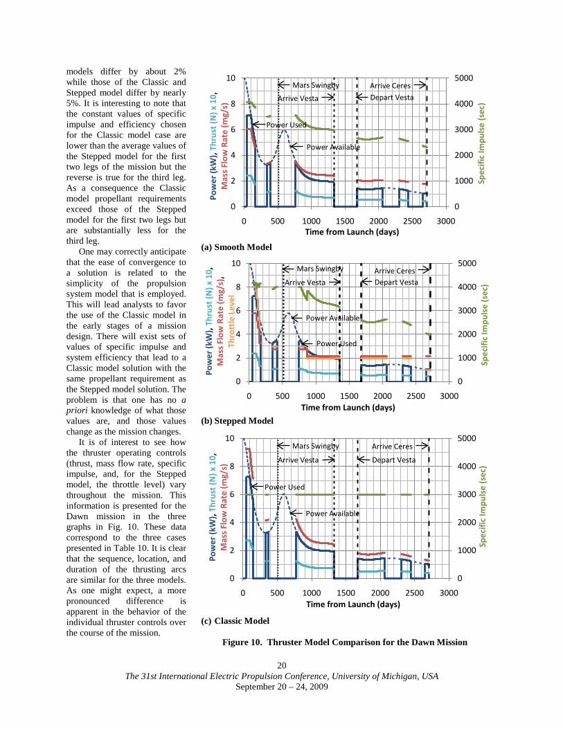
Comparative performance data for the Dawn mission and the three propulsion modeling options available in HILTOP are presented in Table 10. These results are fairly typical, but can be much larger or much smaller if one takes care in defining the operating characteristics of the Smooth and Classic models to better match the tabular performance parameters of the Stepped option. The total propellant mass requirements for the Smooth and Stepped

Table 10. Propulsion Model Comparison for Dawn Mission

Parameter Smooth Stepped Classic Leg 1 Earth-Mars Launch date 9/27/2007 9/27/2007 9/27/2007 Launch C3 (km2/s2) 5.2285 5.3741 4.9628 Launch declination (deg) 28.5 28.5 28.5 Launch mass (kg) 1,105.2 1,101.7 1,111.3 Flight time (days) 510 510 510 Arrival mass (kg) 1,032.7 1,030.4 1019.7 Propellant used (kg) 72.4 71.3 91.6 Leg 2 Mars-Vesta Swingby date 2/18/2009 2/18/2009 2/18/2009 Swingby v∞ (km/s) 4.11 3.86 4.26 Passage altitude (km) 300 300 300 Flight time (days) 827.7 850.5 818.56 Arrival date 5/26/2011 6/19/2011 5/18/2011 Arrival mass (kg) 901.4 909.5 885.1 Propellant used (kg) 131.3 120.9 134.6 Stay time (days) 336.3 313.5 345.4 Leg 3 Vesta-Ceres Departure date 4/27/2012 4/27/2012 4/27/2012 Flight time (days) 1,038 1,038 1,038 Arrival date 2/28/2015 2/28/2015 2/28/2015 Arrival mass (kg) 802.3 804.9 799.9 Propellant used (kg) 99.1 104.6 85.3 Total Propellant (kg) 302.8 296.8 311.4 Mission duration (days) 2,711 2,711 2,711


September 20 – 24, 2009

20

models differ by about 2% while those of the Classic and Stepped model differ by nearly 5%. It is interesting to note that the constant values of specific impulse and efficiency chosen for the Classic model case are lower than the average values of the Stepped model for the first two legs of the mission but the reverse is true for the third leg. As a consequence the Classic model propellant requirements exceed those of the Stepped model for the first two legs but are substantially less for the third leg.

One may correctly anticipate that the ease of convergence to a solution is related to the simplicity of the propulsion system model that is employed. This will lead analysts to favor the use of the Classic model in the early stages of a mission design. There will exist sets of values of specific impulse and system efficiency that lead to a Classic model solution with the same propellant requirement as the Stepped model solution. The problem is that one has no a priori knowledge of what those values are, and those values change as the mission changes.

It is of interest to see how the thruster operating controls (thrust, mass flow rate, specific impulse, and, for the Stepped model, the throttle level) vary throughout the mission. This information is presented for the Dawn mission in the three graphs in Fig. 10. These data correspond to the three cases presented in Table 10. It is clear that the sequence, location, and duration of the thrusting arcs are similar for the three models. As one might expect, a more pronounced difference is apparent in the behavior of the individual thruster controls over the course of the mission.

(a) Smooth Model

(b) Stepped Model

(c) Classic Model

Figure 10. Thruster Model Comparison for the Dawn Mission

0

1000

2000

3000

4000

5000

0

2

4

6

8

10

0 500 1000 1500 2000 2500 3000

Spec

ific

Impu

lse

(sec

)

Pow

er (k

W),

Thru

st (N

) x 1

0,

Mas

s Fl

ow R

ate

(mg/

s)Time from Launch (days)

Mars Swingby Arrive Ceres

Arrive Vesta Depart Vesta

Power Used

Power Available

0

1000

2000

3000

4000

5000

0

2

4

6

8

10

0 500 1000 1500 2000 2500 3000

Spec

ific

Impu

lse

(sec

)

Pow

er (k

W),

Thru

st (N

) x 1

0,

Mas

s Fl

ow R

ate

(mg/

s),

Thro

ttle

Lev

el


Mars Swingby Arrive CeresArrive Vesta Depart Vesta

Power Available

Power Used

0

1000

2000

3000

4000

5000

0

2

4

6

8

10

0 500 1000 1500 2000 2500 3000

Spec

ific

Impu

lse

(sec

)

Pow

er (k

W),

Thru

st (N

) x 1

0,

Mas

s Fl

ow R

ate

(mg/

s)


Mars Swingby

Arrive Vesta

Arrive Ceres

Depart Vesta

Power Used

Power Available


September 20 – 24, 2009

21

VI. Conclusion Features of the newly revised and rewritten low-thrust trajectory optimization program HILTOP have been

described and its capabilities were placed in context with those of alternative software programs currently in use within NASA and the space community. Optimal trajectory solutions of four complex space exploration missions of current interest were obtained with the program and compared to solutions obtained with the MALTO program, a medium fidelity low-thrust trajectory optimization program that is part of NASA’s Low-Thrust Trajectory Tool suite of mission analysis software. The relatively minor differences in the performance requirements identified by the two programs were primarily attributable to differences in analytic models such as launch vehicle payload capabilities and low-thrust planetary orbit escape and capture algorithms. For the most complex of the four missions studied, a nine-year Saturn flyby mission that employs a Venus swingby and three Earth swingbys, the final mass at Saturn for the two solutions differed by only 0.01%. It is concluded that the two programs validate each other and, by virtue of the fact that MALTO was previously validated against other tools in the LTTT suite and with NASA legacy software, HILTOP can be used with a high level of confidence that its results are reproducible with alternative software products available within the industry. The success achieved with HILTOP in developing optimal solutions for highly complex, multi-target missions also provides evidence of the viability of indirect methods for the optimization of space exploration missions of current interest. Both HILTOP and MALTO are rich in features sought by mission analysts and may well prove to be complimentary rather than competitive in their application.

References

1”Mathematical Model for HILTOP, Heliocentric Interplanetary Low-thrust Trajectory Optimization Program, Version 2.1,” January 2009 2” HILTOP User Guide, Heliocentric Interplanetary Low-thrust Trajectory Optimization Program, Version 2.1,” January 2009 3Polsgrove, T., Kos, L., and Hopkins, R., “Comparison of Performance Predictions for New Low-Thrust Trajectory Tools,” AIAA 2006-6742, presented at the AIAA/AAS Astrodynamics Specialist Conference and Exhibit, Keystone, Colorado, August 2006. 4Kos, L. D., Polsgrove, T., Hopkins, R. C., and Thomas, D., “Overview of the Development for a Suite of Low-Thrust Trajectory Analysis Tools,” AIAA 2006-6743, presented at the AIAA/AAS Astrodynamics Specialist Conference and Exhibit, Keystone, Colorado, August 2006. 5Sims, J. A., Finlayson, P. A., Rinderle, E. A., Vavrina, M. A., and Kowalkowski, T. D., “Implementation of a Low-Thrust Trajectory Optimization Algorithm for Preliminary Design,” AIAA 2006-6746, presented at the AIAA/AAS Astrodynamics Specialist Conference and Exhibit, Keystone, Colorado, August 2006.

Documents

Heliocentric Interplanetary Low-thrust Trajectory