Embed Size (px)
Citation preview

Central European University
Department of Mathematics and its Application
Heegaard Floer Invariantsof Smooth and Legendrian Links
inRational Homology 3-spheres
by
Alberto Cavallo
SupervisorProf. András I. Stipsicz
BUDAPEST, HUNGARY
2018
CE
UeT
DC
olle
ctio
n

CE
UeT
DC
olle
ctio
n

Declaration
I hereby declare that this dissertation contains no materials accepted for any other de-grees in any other institutions.
Moreover, the dissertation contains no materials previously written and/or publishedby another person, except where appropriate acknowledgment is made in the form ofbibliographical reference.
Budapest, April 10 2018 Alberto Cavallo
iii
CE
UeT
DC
olle
ctio
n

CE
UeT
DC
olle
ctio
n

Abstract
Our main goal in this thesis is to describe the most important results on smooth andLegendrian knots obtained from Heegaard Floer homology in the last ten years and gen-eralize some of them to links.
Our first result is a link version of the Thurston-Bennequin inequality. This inequality,in its usual formulation, gives an upper bound for the maximal Thurston-Bennequin andself-linking numbers of a knot K in a tight contact 3-manifolds (M, ξ), in terms of the Eulercharacteristic of a Seifert surface for K. We generalize the inequality to every link L, wherethe resulting upper bound involves the Thurston norm of L. This is a rational numberextracted from the semi-norm, introduced by Thurston, on the relative second homologygroup of a 3-manifold with toric boundary.
We say that two n-component links in S3 are strongly concordant if there is a cobordismbetween them consisting of n disjoint annuli, each one realizing a knot concordance. Then,starting from a grid diagram D of a link L, we define a filtered chain complex
(GC(D), ∂
)and we prove that its homology, denoted with HFL(L), is a strong concordance invariant.
Since we can prove that HFL(L) has dimension one in Maslov grading zero, we alsoextract a numerical invariant from the homology group that we call τ(L). The τ-invariantgives a lower bound for the slice genus g4(L), which is the minimum genus of an oriented,compact surface properly embedded in D4 and whose boundary is L. We also show thatthere is a strict relation between the filtration levels of HFL(L) and the Alexander grad-ing of the torsion-free quotient of cHFL−(L), a different bigraded version of link Floerhomology.
Furthermore, we define an invariant of Legendrian links by using open book decom-positions. This is done by describing a suitable condition for an open book decomposition(B, π, A) to be adapted to a Legendrian link L, where A is a system of generators of thefirst relative homology group of π−1(1). At this point, we define a special Heegaard dia-gram D for the link L in the 3-manifold −M, given by reversing the orientation on M; wehave that D is obtained up to isotopy from (B, π, A) and then, when L is zero in homology,the invariant L(L, M, ξ) is the isomorphism class of a distinguished cycle L(D) in the linkFloer complex cCFL−(D, tξ).
We also give some results on quasi-positive links in S3. In particular, we introducethe subfamily of connected transverse C-links: these are links such that the surface ΣB,associated to a quasi-positive braid B for L, is connected. We show that, for this kind oflinks, the slice genus g4 is determined by τ. This allows us to prove that the slice genus isadditive under connected sums of connected transverse C-links.
v
CE
UeT
DC
olle
ctio
n

CE
UeT
DC
olle
ctio
n

Contents
Introduction 3
Acknowledgements 7
1 Preliminaries 91.1 Knots and links in 3-manifolds . . . . . . . . . . . . . . . . . . . . . . . . . . 9
1.1.1 Definition of links . . . . . . . . . . . . . . . . . . . . . . . . . . . . . . 91.1.2 Connected sum and mirror image of links . . . . . . . . . . . . . . . . 10
1.2 Links in the 3-sphere . . . . . . . . . . . . . . . . . . . . . . . . . . . . . . . . 111.2.1 Diagrams for links in S3 . . . . . . . . . . . . . . . . . . . . . . . . . . 111.2.2 The Seifert algorithm . . . . . . . . . . . . . . . . . . . . . . . . . . . . 121.2.3 Operations on links and planar diagrams . . . . . . . . . . . . . . . . 14
1.3 Cobordisms . . . . . . . . . . . . . . . . . . . . . . . . . . . . . . . . . . . . . 151.3.1 Definition of cobordism and the slice genus . . . . . . . . . . . . . . . 151.3.2 Link concordance . . . . . . . . . . . . . . . . . . . . . . . . . . . . . . 16
1.4 Filtered chain complexes . . . . . . . . . . . . . . . . . . . . . . . . . . . . . . 181.4.1 Filtered spaces ... . . . . . . . . . . . . . . . . . . . . . . . . . . . . . . 181.4.2 ... and filtered maps . . . . . . . . . . . . . . . . . . . . . . . . . . . . 19
1.5 Tensor product of modules . . . . . . . . . . . . . . . . . . . . . . . . . . . . . 211.5.1 General properties and vector spaces . . . . . . . . . . . . . . . . . . 211.5.2 Finitely generated K[x]-modules . . . . . . . . . . . . . . . . . . . . . 22
2 The Thurston norm 252.1 Definition . . . . . . . . . . . . . . . . . . . . . . . . . . . . . . . . . . . . . . 252.2 Results . . . . . . . . . . . . . . . . . . . . . . . . . . . . . . . . . . . . . . . . 28
3 Contact structures and Legendrian links 313.1 Contact structures . . . . . . . . . . . . . . . . . . . . . . . . . . . . . . . . . . 31
3.1.1 Type of structures and convex surfaces . . . . . . . . . . . . . . . . . 313.1.2 Classification theorems . . . . . . . . . . . . . . . . . . . . . . . . . . 323.1.3 Fillings . . . . . . . . . . . . . . . . . . . . . . . . . . . . . . . . . . . . 33
3.2 Legendrian links . . . . . . . . . . . . . . . . . . . . . . . . . . . . . . . . . . 343.3 Transverse links . . . . . . . . . . . . . . . . . . . . . . . . . . . . . . . . . . . 363.4 Legendrian and transverse links in (S3, ξst) . . . . . . . . . . . . . . . . . . . 37
3.4.1 Front projections of Legendrian links . . . . . . . . . . . . . . . . . . 373.4.2 Braid presentation for transverse links . . . . . . . . . . . . . . . . . . 38
3.5 Connected sum and disjoint union in the contact setting . . . . . . . . . . . . 403.6 The Thurston-Bennequin inequality . . . . . . . . . . . . . . . . . . . . . . . 42
vii
CE
UeT
DC
olle
ctio
n

4 Representations of links and 3-manifolds 454.1 Heegaard diagrams . . . . . . . . . . . . . . . . . . . . . . . . . . . . . . . . . 45
4.1.1 3-manifolds and Spinc structures . . . . . . . . . . . . . . . . . . . . . 454.1.2 Links . . . . . . . . . . . . . . . . . . . . . . . . . . . . . . . . . . . . . 47
4.2 Open book decompositions . . . . . . . . . . . . . . . . . . . . . . . . . . . . 504.2.1 Adapted open book decompositions for links in 3-manifolds . . . . . 504.2.2 Abstract open books . . . . . . . . . . . . . . . . . . . . . . . . . . . . 53
5 Heegaard Floer homology 575.1 Link Floer homology . . . . . . . . . . . . . . . . . . . . . . . . . . . . . . . . 57
5.1.1 Heegaard diagrams and J-holomorphic curves . . . . . . . . . . . . . 575.1.2 Gradings . . . . . . . . . . . . . . . . . . . . . . . . . . . . . . . . . . . 585.1.3 Differential . . . . . . . . . . . . . . . . . . . . . . . . . . . . . . . . . 615.1.4 Homology . . . . . . . . . . . . . . . . . . . . . . . . . . . . . . . . . . 63
5.2 Heegaard Floer homology of 3-manifolds . . . . . . . . . . . . . . . . . . . . 645.3 Invariance . . . . . . . . . . . . . . . . . . . . . . . . . . . . . . . . . . . . . . 66
5.3.1 Choice of the almost-complex structures . . . . . . . . . . . . . . . . 665.3.2 Isotopies . . . . . . . . . . . . . . . . . . . . . . . . . . . . . . . . . . . 685.3.3 Handleslides . . . . . . . . . . . . . . . . . . . . . . . . . . . . . . . . 695.3.4 Stabilizations . . . . . . . . . . . . . . . . . . . . . . . . . . . . . . . . 70
5.4 Multiplication by U + 1 in the link Floer homology group . . . . . . . . . . . 70
6 Legendrian and contact invariants from open book decompositions 736.1 Legendrian Heegaard diagrams . . . . . . . . . . . . . . . . . . . . . . . . . . 73
6.1.1 Heegaard diagrams through abstract open books . . . . . . . . . . . 736.1.2 Global isotopies . . . . . . . . . . . . . . . . . . . . . . . . . . . . . . . 746.1.3 Positive stabilizations . . . . . . . . . . . . . . . . . . . . . . . . . . . 746.1.4 Admissible arc slides . . . . . . . . . . . . . . . . . . . . . . . . . . . . 77
6.2 The Legendrian and transverse invariants . . . . . . . . . . . . . . . . . . . . 806.3 Proof of the invariance . . . . . . . . . . . . . . . . . . . . . . . . . . . . . . . 81
6.3.1 Global isotopies and admissible arc slides . . . . . . . . . . . . . . . . 816.3.2 Invariance under positive stabilizations . . . . . . . . . . . . . . . . . 826.3.3 Invariance theorems . . . . . . . . . . . . . . . . . . . . . . . . . . . . 83
6.4 A remark on the Ozsváth-Szabó contact invariant . . . . . . . . . . . . . . . 846.5 Properties of L and T . . . . . . . . . . . . . . . . . . . . . . . . . . . . . . . . 866.6 Connected sums and invariance of T . . . . . . . . . . . . . . . . . . . . . . . 88
6.6.1 Behaviour of the invariants under connected sum . . . . . . . . . . . 886.6.2 Naturality and a refinement for L . . . . . . . . . . . . . . . . . . . . 92
7 Loose and non-loose links 957.1 Legendrian links in overtwisted structures . . . . . . . . . . . . . . . . . . . 957.2 A classification theorem for loose knots . . . . . . . . . . . . . . . . . . . . . 977.3 Existence of non-loose links with loose components . . . . . . . . . . . . . . 997.4 Non-simple link types . . . . . . . . . . . . . . . . . . . . . . . . . . . . . . . 103
viii
CE
UeT
DC
olle
ctio
n

8 Link Floer homology and grid diagrams 1058.1 Filtered simply blocked link grid homology . . . . . . . . . . . . . . . . . . . 105
8.1.1 The chain complex . . . . . . . . . . . . . . . . . . . . . . . . . . . . . 1058.1.2 The differential . . . . . . . . . . . . . . . . . . . . . . . . . . . . . . . 1078.1.3 The homology . . . . . . . . . . . . . . . . . . . . . . . . . . . . . . . . 1078.1.4 Equivalence between GH and HFL . . . . . . . . . . . . . . . . . . . 108
8.2 The invariant tau in the filtered theory . . . . . . . . . . . . . . . . . . . . . . 1098.2.1 Definition of the invariant . . . . . . . . . . . . . . . . . . . . . . . . . 1098.2.2 Dropping the special O-markings . . . . . . . . . . . . . . . . . . . . 1118.2.3 Symmetries . . . . . . . . . . . . . . . . . . . . . . . . . . . . . . . . . 112
8.3 Cobordisms . . . . . . . . . . . . . . . . . . . . . . . . . . . . . . . . . . . . . 1158.3.1 Induced maps and degree shift . . . . . . . . . . . . . . . . . . . . . . 1158.3.2 Strong concordance invariance . . . . . . . . . . . . . . . . . . . . . . 1208.3.3 A lower bound for the slice genus . . . . . . . . . . . . . . . . . . . . 121
8.4 TheHFL− version of the homology . . . . . . . . . . . . . . . . . . . . . . . 1238.4.1 A different point of view . . . . . . . . . . . . . . . . . . . . . . . . . . 1238.4.2 Filtered link homology and the τ-set . . . . . . . . . . . . . . . . . . . 124
8.5 Applications . . . . . . . . . . . . . . . . . . . . . . . . . . . . . . . . . . . . . 1268.5.1 Computation for some specific links . . . . . . . . . . . . . . . . . . . 1268.5.2 Torus links . . . . . . . . . . . . . . . . . . . . . . . . . . . . . . . . . . 1278.5.3 Applications to Legendrian invariants . . . . . . . . . . . . . . . . . . 128
9 Quasi-positive links in the 3-sphere 1319.1 Maximal self-linking number and the slice genus . . . . . . . . . . . . . . . . 1319.2 Strongly quasi-positive links . . . . . . . . . . . . . . . . . . . . . . . . . . . . 1349.3 The case of positive links . . . . . . . . . . . . . . . . . . . . . . . . . . . . . . 136
Bibliography 141
Index 146
ix
CE
UeT
DC
olle
ctio
n

CE
UeT
DC
olle
ctio
n

List of Figures
1.1 Meridian curve along a knot . . . . . . . . . . . . . . . . . . . . . . . . . . . . 101.2 Elementary tangles . . . . . . . . . . . . . . . . . . . . . . . . . . . . . . . . . 111.3 Positive trefoil knot . . . . . . . . . . . . . . . . . . . . . . . . . . . . . . . . . 111.4 Crossing signs in a link diagram . . . . . . . . . . . . . . . . . . . . . . . . . 121.5 Reidemeister moves . . . . . . . . . . . . . . . . . . . . . . . . . . . . . . . . 121.6 Orientation preserving resolutions of crossings . . . . . . . . . . . . . . . . . 131.7 Oriented resolutions of link diagrams . . . . . . . . . . . . . . . . . . . . . . 131.8 Connected sum of knots . . . . . . . . . . . . . . . . . . . . . . . . . . . . . . 141.9 Figure-eight knot . . . . . . . . . . . . . . . . . . . . . . . . . . . . . . . . . . 141.10 Elementary cobordisms . . . . . . . . . . . . . . . . . . . . . . . . . . . . . . 151.11 Morse moves . . . . . . . . . . . . . . . . . . . . . . . . . . . . . . . . . . . . . 151.12 Strong cobordism between the Whitehead link and the unlink . . . . . . . . 161.13 Positive Hopf link . . . . . . . . . . . . . . . . . . . . . . . . . . . . . . . . . . 17
2.1 2-handle attachment on genus 1 handlebody . . . . . . . . . . . . . . . . . . 28
3.1 Standard Legendrian unknot in (S3, ξst) . . . . . . . . . . . . . . . . . . . . . 383.2 Legendrian Reidemeister moves . . . . . . . . . . . . . . . . . . . . . . . . . 383.3 A generator of the group of k-braids . . . . . . . . . . . . . . . . . . . . . . . 393.4 Trivial elementary Legendrian tangle . . . . . . . . . . . . . . . . . . . . . . . 413.5 Stabilizations of the standard Legendrian unknot in (S3, ξst) . . . . . . . . . 413.6 Disjoint union of Legendrian links . . . . . . . . . . . . . . . . . . . . . . . . 41
4.1 Genus one Heegaard diagram for S3 . . . . . . . . . . . . . . . . . . . . . . . 454.2 Handleslide move on Heegaard diagrams . . . . . . . . . . . . . . . . . . . . 464.3 Stabilization move on Heegaard diagrams . . . . . . . . . . . . . . . . . . . . 464.4 Genus zero Heegaard diagram for the unlink©2 in S3 . . . . . . . . . . . . 484.5 System of generators on a planar surface adapted to a link . . . . . . . . . . 514.6 Separating arc on a page of an open book decomposition-1 . . . . . . . . . . 524.7 Separating arc on a page of an open book decomposition-2 . . . . . . . . . . 534.8 A strip on a page of an open book decomposition . . . . . . . . . . . . . . . 544.9 Basepoints on a page of an open book decomposition . . . . . . . . . . . . . 544.10 Orientation induced by the basepoints . . . . . . . . . . . . . . . . . . . . . . 55
5.1 Domains in the underlying surface of a Heegaard diagram . . . . . . . . . . 585.2 Stabilization with an unknotted component . . . . . . . . . . . . . . . . . . . 655.3 Isotopy on a Heegaard diagram . . . . . . . . . . . . . . . . . . . . . . . . . . 68
6.1 Legendrian Heegaard diagram of a Legendrian unlink . . . . . . . . . . . . 73
xi
CE
UeT
DC
olle
ctio
n

6.2 Positive stabilization of an abstract open book . . . . . . . . . . . . . . . . . 756.3 Reducing the twisting of ξ along a curve in the page of an open book de-
composition . . . . . . . . . . . . . . . . . . . . . . . . . . . . . . . . . . . . . 756.4 Splitting a 2-cell in a contact cell decomposition . . . . . . . . . . . . . . . . 766.5 Admissible arc slide on the page of an abstract open book . . . . . . . . . . . 776.6 Separating arcs-1 . . . . . . . . . . . . . . . . . . . . . . . . . . . . . . . . . . 786.7 Separating arcs-2 . . . . . . . . . . . . . . . . . . . . . . . . . . . . . . . . . . 796.8 Separating arcs-3 . . . . . . . . . . . . . . . . . . . . . . . . . . . . . . . . . . 796.9 A stabilized Legendrian Heegaard diagram for a contact 3-manifold . . . . 866.10 Murasugi sum of abstract open books-1 . . . . . . . . . . . . . . . . . . . . . 896.11 Murasugi sum of abstract open books-2 . . . . . . . . . . . . . . . . . . . . . 89
7.1 A non-loose Legendrian link with non-loose components . . . . . . . . . . . 967.2 Loose Legendrian knots and overtwisted disks . . . . . . . . . . . . . . . . . 987.3 Legendrian knots with non-zero Legendrian invariant in contact 3-spheres-1 1007.4 Legendrian knots with non-zero Legendrian invariant in contact 3-spheres-2 1017.5 A connected sum of multiple Legendrian Hopf links . . . . . . . . . . . . . . 102
8.1 Grid diagram for the positive trefoil knot . . . . . . . . . . . . . . . . . . . . 1068.2 Adding a disjoint unknot to a link . . . . . . . . . . . . . . . . . . . . . . . . 1108.3 Cobordism with no critical points . . . . . . . . . . . . . . . . . . . . . . . . . 1168.4 Cobordisms with an index one critical point . . . . . . . . . . . . . . . . . . . 1168.5 Band move in a grid diagram . . . . . . . . . . . . . . . . . . . . . . . . . . . 1178.6 Cobordism with two index one critical points . . . . . . . . . . . . . . . . . . 1178.7 Cobordism with an index zero critical point . . . . . . . . . . . . . . . . . . . 1188.8 Cobordism with an index zero and an index one critical points . . . . . . . . 1188.9 Birth move in a grid diagram . . . . . . . . . . . . . . . . . . . . . . . . . . . 1198.10 Snail-like domains in a grid diagram . . . . . . . . . . . . . . . . . . . . . . . 1198.11 Cobordism with an index one and an index two critical points . . . . . . . . 1208.12 Canonical form of a cobordism between two links . . . . . . . . . . . . . . . 1218.13 O-markings in a grid diagram-1 . . . . . . . . . . . . . . . . . . . . . . . . . . 1268.14 O-markings in a grid diagram-2 . . . . . . . . . . . . . . . . . . . . . . . . . . 1278.15 Grid diagram for a positive torus link . . . . . . . . . . . . . . . . . . . . . . 1278.16 Link L9n
19 . . . . . . . . . . . . . . . . . . . . . . . . . . . . . . . . . . . . . . . 1298.17 Link L9a
40 . . . . . . . . . . . . . . . . . . . . . . . . . . . . . . . . . . . . . . . 130
9.1 Surface associated to a quasi-positive braid . . . . . . . . . . . . . . . . . . . 1319.2 Quasi-positive surface (4, (σ13, σ24, σ13, σ24)) . . . . . . . . . . . . . . . . . . . 1349.3 Transverse realization of a strongly quasi-positive link . . . . . . . . . . . . . 1359.4 Legendrianization of a positive link . . . . . . . . . . . . . . . . . . . . . . . 138
xii
CE
UeT
DC
olle
ctio
n

CE
UeT
DC
olle
ctio
n

CE
UeT
DC
olle
ctio
n

( ... ) while a cloud of smokesettled heavily over thebattlements in the distinctcolossal figure of-a horse.
E. A. Poe
CE
UeT
DC
olle
ctio
n

CE
UeT
DC
olle
ctio
n

Introduction
In the early years of the 21st century, Ozsváth and Szabó introduced an invariant [68],that they decided to call Heegaard Floer homology, which had a great impact in the studyof low dimensional topology. This is an invariant of 3-manifolds up to diffeomorphism; itis obtained from a particular presentation of the 3-manifold M, called a Heegaard diagram,consisting of a closed, oriented, genus g surface Σ, together with two sets α and β of gindependent, disjoint, simple closed curves and a basepoint w in Σ.
A chain complex over F, the field with two elements, can be associated to a Heegaarddiagram, where the generators are combinatorially defined from α and β. The differentialis gotten by counting J-holomorphic disks in the g-fold symmetric power of Σ, equippedwith an almost-complex structure J, as we explain in Subsection 4.1.1. The Heegaard Floerhomology group is the homology of this chain complex. There exist many different ver-sions of the homology, depending on how many J-holomorphic disks we take into account,but all of them are invariants of M. One of the most useful, that we define in Section 5.2, isdenoted with HF(M).
Heegaard Floer homology groups possess an F-splitting induced by Spinc structures.Using a definition of Turaev in [88], we say that a Spinc structure on M is the homotopyclass, away from a point, of a 2-plane field on M. This means that we can write a summandof HF(M) as HF(M, t), where t is a Spinc structure on M.
Moreover, we have an additional grading, called Maslov grading, in the case whensome conditions are satisfied; more specifically, we require the first Chern class of t to bea torsion class. This always happens if M is a rational homology 3-sphere, which is a3-manifold with rational homology isomorphic to the one of the 3-sphere S3; in fact, inthis case the second integer cohomology group is a finite group. For this reason, and thefact that many proofs are easier in this setting, we suppose that 3-manifolds are rationalhomology spheres unless the converse is explicitly written.
Ozsváth and Szabó found a way to extend Heegaard Floer homology to an invariantof links in 3-manifolds [69], in this setting called link Floer homology. This was discoveredindependently by Rasmussen in his doctoral thesis [78].
Moreover, in [70] they use it to define an invariant of contact 3-manifolds. A contactstructure ξ on M is a cooriented 2-plane field, given as the kernel of a 1-form α on M, suchthat α ∧ dα is a volume form for M. We say that ξ is overtwisted if there is an embeddeddisk E in M whose boundary is a Legendrian knot, which means that at each point thetangent vector is contained in the contact structure, and the contact framing of ∂E haszero twisting along E. The last sentence can be rephrased by saying that the Thurston-Bennequin number of ∂E is equals to zero, see Chapter 3. We say that the structure ξ istight if it is not overtwisted.
In [70] the contact invariant c(M, ξ) is defined. This is done by identifying the isomor-phism class of an element in the group HF(M, tξ), where tξ is the Spinc structure induced
3
CE
UeT
DC
olle
ctio
n

by ξ. The class c(M, ξ) is a contact isotopy invariant of (M, ξ). One of its applicationsconsists of a simpler proof of a well-known result of Eliashberg and Gromov in [25], whichsays that a symplectically fillable contact structure on a rational homology sphere is alwaystight.
A contact strucutre ξ is weakly symplectically fillable if there is a compact symplectic4-manifold (X, ω) such that ∂X = M and ω|ξ> 0. It follows from [70] that c(M, ξ) vanishesif ξ is overtwisted, while the contact invariant is non-trivial when the contact structure issymplectically fillable.
Our main goal in this thesis is to describe, in the best way we can, the most importantresults on smooth and Legendrian knots obtained from Heegaard Floer homology in thelast ten years and generalize some of them to links.
After giving some background on smooth links in 3-manifolds and contact topologyin Chapters 1 and 3 respectively, we prove our first result: a link version of the Thurston-Bennequin inequality. This inequality, in its usual formulation, gives an upper bound forthe maximal Thurston-Bennequin and self-linking numbers of a knot K in a tight contact3-manifold (M, ξ), in terms of the Euler characteristic of a Seifert surface for K. A proof ofthe Thurston-Bennequin inequality for null-homologous knots was given by Eliashberg in[23]. We apply the same strategy, already used by Baker and Etnyre [2], to generalize theinequality to every link L, see Section 3.6, where the resulting upper bound involves theThurston norm of L.
We define the Thurston norm ‖L‖T for every link in a rational homology sphere inChapter 2; it is a rational number extracted from the semi-norm, introduced by Thurstonin [86], on the relative second homology group of a 3-manifold with toric boundary. Aresult of Ni [62] and Ozsváth and Szabó [73] implies that link Floer homology detects‖L‖T. The results on the Thurston-Bennequin inequality and the Thurston norm appear in[12].
The computation of link Floer homology in the J-holomorphic setting happens to bevery hard. To solve this problem, in [58] Manolescu, Ozsváth, Szabó and Thurston find acombinatorial reformulation of the homology, in terms of grid diagrams. These are gridsof squares, that were already known in the 19th century, which can also be used to presentlinks in S3.
We say that two n-component links in S3 are strongly concordant if there is a cobordismbetween them consisting of n disjoint annuli, each one realizing a knot concordance. Then,starting from a grid diagram D of a link L, we define a filtered chain complex
(GC(D), ∂
)and we prove in Section 8.3 that its homology, denoted with HFL(L), is a strong concor-dance invariant. Our claim is similar to a result of Pardon [74] about Lee homology.
Since we can prove that HFL(L) has dimension one in Maslov grading zero, we alsoextract a numerical invariant from the homology group that we call τ(L) because, in thecase of knots, it coincides with the concordance invariant introduced by Ozsváth and Sz-abó in [69]. The τ-invariant gives a lower bound for the slice genus g4(L), which is theminimum genus of an oriented, compact surface properly embedded in D4 and whoseboundary is L; see Subsection 8.3.3.
In Chapter 8 we also show that there is a strict relation between the filtration levels ofHFL(L) and the Alexander grading of the torsion-free quotient of cHFL−(L), a differentbigraded version of link Floer homology introduced in [67, 72]. The results about the τ-invariant and link Floer homology appear in [9].
4
CE
UeT
DC
olle
ctio
n

In Chapter 4 we talk in detail about Heegaard diagrams. More specifically, we describehow to construct such a diagram starting from a link L in a 3-manifold M and we showhow to relate two diagrams representing smoothly isotopic links in M. As we remarkedbefore, Heegaard diagrams play a crucial role in the definition of Heegaard and link Floerhomology, see also Chapter 5, but in the case that M is equipped with a contact structure ξand L is Legendrian, we need to use a different presentation, which takes into account thecontact information.
For this reason we introduce open book decompositions. Given a contact 3-manifold(M, ξ), this is a pair (B, π) where B is a smooth link in M and π is a locally trivial fibrationof M \ B onto S1, such that the closures of the fibers have B as boundary. When somecompatibility conditions, described in Section 4.2, are satisfied, we say that (B, π) supportsthe structure ξ.
In [57] Lisca, Ozsváth, Stipsicz and Szabó define open book decompositions (B, π, A),adapted to a Legendrian knot K, by also requiring that K is contained in S1 = π−1(1)and A is an appropriate basis of the relative first homology group of S1. In this way theyconstruct the Legendrian knot invariant L(K, M, ξ) by applying a result in [47].
We extend this invariant to every Legendrian link L in Section 6.1. This is done bydescribing a suitable condition for an open book decomposition (B, π, A) to be adapted toL; this time the set A is not a basis anymore, but only a system of generators, the details ofthe construction are given in Subsection 4.2.1. At this point, we define a special Heegaarddiagram D, that we call a Legendrian Heegaard diagram, for the link L in the 3-manifold−M, given by reversing the orientation on M; we have that D is obtained up to isotopyfrom (B, π, A) and then, when L is zero in homology, the invariant L(L, M, ξ) is the iso-morphism class of a distinguished cycle L(D) in the link Floer complex cCFL−(D, tξ). Inparticular, the invariant L(L, M, ξ) can be seen as an isomorphism class in the homologygroup cHFL−(−M, L, tξ). All the details can be found in Chapter 6.
We have that L(L, M, ξ) is a Legendrian link invariant in the following sense. If L1 andL2 are Legendrian isotopic links in (M, ξ) then, given Legendrian Heegaard diagrams Direpresenting Li for i = 1, 2, we can find a chain map between cCFL−(D1) and cCFL−(D2)which sends L(D1) into L(D2), see Section 6.3.
In [3] Baldwin, Vela-Vick and Vértesi, using a different construction, introduce anotherinvariant of Legendrian links in contact 3-manifolds which generalizes L in the case ofknots in the standard 3-sphere. The same argument in [3] implies that this invariant coin-cides with our L for every Legendrian link in (S3, ξst).
Furthermore, our invariant has the same property of its knot version in [57] regard-ing loose and non-loose links. We say that a Legendrian link L in an overtwisted contactstructure is non-loose if its complement is tight, while it is loose if its complement is over-twisted. We prove in Section 7.1 that L(L, M, ξ) vanishes when L is loose. This result givesa sufficient condition for L to be non-loose. In fact, in Chapter 7 it allows us to provethe existence of a non-split, non-loose n-component Legendrian link in every overtwistedstructure on S3. Moreover, using a naturality property of connected sums, we are also ableto distinguish two non-loose Legendrian links L1 and L2 with the same classical invariants(link type and Thurston-Bennequin and rotation numbers) and Legendrian isotopic com-ponents. In other words, we say that the link type of L1 and L2 is non-loose non-simple.The results about the invariant L and adapted open book decompositions appear in [10].
The invariant L seems to give less information in the case of loose links. In fact, we havesome results that go in the opposite direction. One of these is a theorem of Dymara, see
5
CE
UeT
DC
olle
ctio
n

[17], which says that two loose knots L1 and L2 in (M, ξ), with the same classical invariants,such that there is an overtwisted disk in M \ (L1 t L2) are always Legendrian isotopic. InSection 7.2 we generalize this theorem as follows. We relax the condition of having anovertwisted disk disjoint from both knots, but we claim that, in order to have a Legendrianisotopy between L1 and L2, we only need the existence of two disjoint overtwisted disks E1and E2 such that Ei is in the complement of Li for i = 1, 2. An example where we can applyour result, but not Dymara’s theorem, is the case of a disjoint union of two non-loose knots;in other words, when M is a contact connected sum of M1 and M2 and Li is a non-looseknot in Mi for i = 1, 2. The proofs of these results appear in [11].
Finally, in Chapter 9 we give some results on quasi-positive links in S3. These are linkswhich are obtained as closures of some particular braids, called quasi-positive braids. Inparticular, we show that we can always compute the maximal self-linking number and theinvariant τ of a quasi-positive link.
Moreover, in Section 9.1 we introduce the subfamily of connected transverse C-links:these are links such that the surface ΣB, associated to a quasi-positive braid B for L, isconnected; see Section 9.1. We show that, for this kind of links, the slice genus g4 is deter-mined by τ. This allows us to prove that the slice genus is additive under connected sumsof connected transverse C-links; a result which follows from [44] for knots, but appears tobe new in the case of links.
Budapest, March 14 2018
6
CE
UeT
DC
olle
ctio
n

Acknowledgements
I would like to thank Paolo Lisca and András Stipsicz for their advice, the many helpfulconversations and the lots of time spent meeting and discussing mathematics.
I want to thank John Etnyre and Brendan Owens for their responsiveness and the helpgiven in these years.
I am grateful to Irena Matkovic for all the time spent together.After a long time, and maybe a lifetime again, I say thank you to my family.
Budapest, March 21 2018
7
CE
UeT
DC
olle
ctio
n

CE
UeT
DC
olle
ctio
n

Chapter 1
Preliminaries
1.1 Knots and links in 3-manifolds
1.1.1 Definition of links
We start with the definition of knots and links. Let us consider a connected, compact,oriented 3-manifold M. Then an n-component link is the image of a smooth embedding of acollection of n disjoint circles into M. We usually denote a link with L ↪→ M. If we orientall the circles then the link L also inherits an orientation. In this thesis we always assumethat a link is oriented, even when this is not explicitly stated. We call a knot a link with onecomponent.
Let L1 and L2 be two links in a 3-manifold M. Then we say that L1 is smoothly isotopicto L2 if there exists a smooth map H : M× I → M such that
1. H(·, t) is a diffeomorphism for every t ∈ I,
2. H(·, 0) = IdM,
3. H(L1, 1) = L2.
When two links are smoothly isotopic we also say that they are equivalent. The trivial knot,which is called the unknot and is denoted with the symbol©, is a knot in M that boundsan embedded disk. The unknot is well-defined in every 3-manifold M, in the sense that allsuch knots are equivalent. See [79].
If a link L is null-homologous in M, which means that the homology class [L] inH1(M; Z) is zero, then it bounds a compact, oriented embedded surface F inside M. Itis easy to see that such a surface can be made connected by adding some tubes and in thiscase we call F a Seifert surface for L. We denote with g3(L) the minimum genus amongall the Seifert surfaces for the link L. Then the following corollary is an immediate conse-quence of this definition.
Corollary 1.1.1 The unknot is the only knot K, up to isotopy, such that g3(K) = 0.
We say that a link L ↪→ M is split if L is the disjoint union of L1 with L2 and there is aseparating, embedded 2-sphere S in M such that S gives the connected sum decompositionM = M1 #S M2 and Li ↪→ Mi for i = 1, 2. When this happens we write L = L1 t L2.Otherwise L is called non-split. Every link L can be written as L1 t ... t Lk where each Li isa non-split link in M. The Li’s are called split components of L.
9
CE
UeT
DC
olle
ctio
n

We recall that a k-manifold Y is a rational homology sphere if Hi(Y; Q) ∼= Hi(Sk; Z) forevery i ∈ Z. Let us take two knots K1 and K2 in M and suppose that the 3-manifold M isa rational homology 3-sphere. Then we can define the rational linking number between K1and K2 as the rational number
lkQ(K1, K2) =F · K2
t=|F t K2|
t;
where F is a compact, oriented surface, properly embedded in MK1 = M \ ˚ν(K1) and suchthat F · µ = PD[µ][F] = t, while t is the order of [K1] in H1(M; Z). Moreover, here [µ] and[K2] are elements of H1(MK1 ; Q) ∼= Q. The curve µ represents the meridian of the knot K1
K1
µ
Figure 1.1: The meridian µ is oriented accordingly to the knot K1.
as shown in Figure 1.1.
Proposition 1.1.2 The linking number is symmetric. Moreover, if K1 is null-homologous in Mthen lkQ(K1, K2) is an integer.
Proof. The symmetry follows from Poincaré-Lefschetz duality. See [43] for details. Onthe other hand, the second claim is implied by the fact that, if t = 1, the linking numbercoincides with the algebraic intersection of a Seifert surface for K1 with the knot K2; whichis clearly an integer.
In the case when J = J1 ∪ ... ∪ Jn and L = L1 ∪ ... ∪ Lm are two links in a rationalhomology sphere M, we define the linking number as
lkQ(J, L) =n
∑i=1
m
∑j=1
lkQ(Ji, Lj) . (1.1)
We observe that the linking number between two components of a link is invariant un-der smooth isotopies. Moreover, if J and L are both null-homologous then we omit thesubscript Q; thus, the linking number is denoted with lk(J, L) and it is an integer fromProposition 1.1.2.
1.1.2 Connected sum and mirror image of links
We define an elementary tangle as a pair (D3, α) such that α ∼= I = [0, 1] and ∂D3 ∩ α =∂α. See Figure 1.2. An elementary tangle is called trivial if it is isotopic, rel boundary, to(D2 × I, {0} × I).
Given two links Li ↪→ Mi for i = 1, 2 we define a connected sum L1 # L2 as follows. LetD1, D2 be two balls such that (Di, Di ∩ Li) are trivial elementary tangles. Then we glue the
10
CE
UeT
DC
olle
ctio
n

α
α
Figure 1.2: Examples of elementary tangles. The one on the right is trivial.
complements of these elementary tangles in Mi using an orientation reversing diffeomor-phism Φ : ∂D1 → ∂D2 in the way that D1 ∩ L1 is identified with D2 ∩ L2, respecting theorientations of the links. The result of this operation is a pair (M1 # M2, L1 # L2), whereL1 # L2 is a connected sum of L1 and L2.
The link L1 # L2 is well-defined up to the choice of the components of Li that intersectthe trivial elementary tangles in the definition. This means that, if we fix a component Kiin Li for i = 1, 2, the link L1 #(K1,K2) L2 is determined up to smooth isotopy. Moreover, ifL1 and L2 are oriented then L1 # L2 is also oriented and, from [55], we have the followingproperties.
Proposition 1.1.3 Once we fix the components of L1 and L2 where we sum the links, the connectedsum is commutative and associative.
Starting from a link L ↪→ M, we can always reverse the orientation of the 3-manifoldM and then L defines a new link when seen as embedded in −M. Now, suppose that themanifold M admits a diffeomorphism i− : M → M which reverses the orientation. Thenin this case the oriented link L∗ = i−(L) is called the mirror image of L.
1.2 Links in the 3-sphere
1.2.1 Diagrams for links in S3
Every link embedded in S3 can be represented by a planar diagram. In fact, first we
Figure 1.3: An oriented diagram for the positive trefoil knot.
observe that a link L ↪→ S3 is also embedded in R3; then we choose an affine 2-subspaceH ⊂ R3, which is diffeomorphic to R2, such that for the corresponding orthogonal projec-tion pH : R3 → H is
• |p−1H (x) ∩ L| 6 1 for every x ∈ H except a finite number of points, called singular
values, where this number is equal to 2;
• the lines tangent to L in the singular values never project to the same line in H.
11
CE
UeT
DC
olle
ctio
n

A proof of the fact that the plane H exists for every link L in S3 can be found in [55]. At thispoint we define a diagram D for L as the image of L under the projection pH. Moreover,
+ −
Figure 1.4: The signs of a crossing in a diagram.
we say that
• a crossing in D is a singular value;
• an arc in D is a line which connects two crossings, possibly the same, one as startingpoint and the other one as end point;
• each crossing contains the information of which arcs are overcrossings or undercross-ings.
When the link is oriented, a sign can be assigned to each crossing in the diagram D, asshown in Figure 1.4.
A theorem of Reidemeister assures us that two links are equivalent if and only theirdiagrams are related by some moves, which are called Reidemeister moves. There are
Type 1 Type 2 Type 3
Figure 1.5: The three Reidemister moves. For each move, we have to consider all thepossible combinations of reflections and orientations.
three types of these moves and they are pictured in Figure 1.5.
Theorem 1.2.1 (Reidemeister) Two links L1 and L2 in S3 are smoothly isotopic if and only if,given D1, D2 diagrams for L1, L2 respectively, the two diagrams D1 and D2 differ by a finite se-quence of Reidemeister moves and planar isotopies.
A proof of this theorem is found in [55].
1.2.2 The Seifert algorithm
In the 3-sphere we have a method which allows us to determine a Seifert surface for agiven oriented link L, starting from a diagram D. We define the oriented resolution of D as
12
CE
UeT
DC
olle
ctio
n

the collection of circles in R2 obtained by resolving all the crossings in D preserving theorientation. It is easy to see that, for each crossing, this can be done only in one possibleway, as shown in Figure 1.6. The circles have the orientation induced on them by D.
From the oriented resolution we can construct a compact, oriented surface F in the3-space which is bounded by the link L. We start by pushing all the circles up, startingfrom the innermost ones, until they are all on different levels and then we take the disksthat they bound. So we now have a collection of disjoint disks in R3. We connect these
Figure 1.6: Examples of orientation preserving resolutions.
disks by attaching negative (positive) bands in correspondence with the positive (negative)crossings in D. The orientation on F is defined in the following way: it coincides with theone induced by R2 on the circles oriented counter-clockwise, while it is the opposite on thecircles oriented clockwise. It is easy to check that such orientation can be extended to thewhole surface F.
Since we can suppose that the resolutions are always performed in a very small neigh-borhood of the crossing, we can connect two circles, in the oriented resolution of D, byadding lines in correspondence with each crossings. In this way we define a planar sub-space D associated to the oriented resolution, as in Figure 1.7. The subspace D is homo-topy equivalent to the 4-valent graph given by D when we remove the under and over-crossings. Moreover, the surface F is connected if and only if its associated planar subspaceis connected. The latter property, in knot theory, is the definition of non-split diagram of a
D
D′
F′
D′
D
Figure 1.7: A diagram and its associated oriented resolution. The surface F′ is obtained byapplying the given algorithm to D′.
link; moreover, it implies the following theorem.
Theorem 1.2.2 (Seifert algorithm) Every diagram D of a link in S3 gives a Seifert surface byapplying the procedure described above.
Proof. When D is non-split, the surface F determined by the oriented resolution of thediagram is a Seifert surface for L for what we say before. If D is split then we need toconnect the components of F together by removing small disks and inserting long, thintubes; at this point the claim follows easily.
13
CE
UeT
DC
olle
ctio
n

1.2.3 Operations on links and planar diagrams
In Subsection 1.1.1 we defined the linking number between two knots. In S3 such
Figure 1.8: A diagram for the connected sum between a negative trefoil knot and a figure-eight knot.
number is always an integer, since the group H1(S3; Z) is trivial, and it is computed easilyusing knot diagrams .
Proposition 1.2.3 Let D1, D2 be diagrams for the oriented knots K1, K2 respectively. Then
lk(K1, K2) = ∑p | D1↑D2
εp ,
where the symbol ↑ means that, at the crossing p, the arc in D1 overcrosses the one in D2 and ε isthe sign of p, according to Figure 1.4.
Proof. It follows easily from the definition of linking number; see [79].
Given a diagram D, we can also define the writhe of D, and we denote it with wr(D),as
wr(D) = ∑p
εp ,
where ε and p are as in Proposition 1.2.3. Here the sum is taken over all the crossings in D.The writhe is not a link invariant, but it has the following property.
Figure 1.9: A diagram for the Figure-eight knot and its mirror image. It is easy to see thatthe two knots are isotopic.
Proposition 1.2.4 The writhe of the diagram D is invariant under Reidemeister 2 and 3 moves,while it changes by ±1 under Reidemeister 1 moves.
Proof. It is enough to check that the claim holds for the moves in Figure 1.5.
14
CE
UeT
DC
olle
ctio
n

Figure 1.8 shows how the connected sum between two links can be seen from planardiagrams . On the other hand, a diagram for the mirror image of L is gotten from a diagramof L by changing the sign of all the crossings. See Figure 1.9.
1.3 Cobordisms
1.3.1 Definition of cobordism and the slice genus
We start this section by giving the definition of cobordism for links in S3. A genus g
Figure 1.10: The standard cobordisms in S3 × I. Each one contains at most one criticalpoint.
cobordism, between links L1 and L2 in the 3-sphere, is the image of a smooth embeddingf : Σg → S3 × I, where Σg is a compact, oriented surface of genus g; more precisely, thesurface Σg has connected components Σg1 , ..., ΣgJ and g = g1 + ... + gJ . Furthermore, we
Birth
Band
Death
Figure 1.11: The three Morse moves. Birth and Death moves consist of creating and delet-ing disjoint unknots.
have that Σg satisfies the following properties:
1. f (∂Σg) = (−L1)× {0} t L2 × {1};
2. f (Σg \ ∂Σg) ⊂ S3 × (0, 1);
3. every connected component of Σg has boundary in both L1 and L2.
In all the figures in this section cobordisms are drawn as standard surfaces in S3, but theycan be knotted in S3 × I.
15
CE
UeT
DC
olle
ctio
n

It is a standard result in Morse theory, see [59], that a link cobordism can be decom-posed into five standard cobordisms, which appear in Figure 1.10. Then this gives a gen-eralization of Reidemeister theorem.
Theorem 1.3.1 Let D1 and D2 be two diagrams for the links L1 and L2 in S3. Then for every cobor-dism Σ, between L1 and L2, the diagram D2 is obtained from D1 by a finite number of Reidemeisterand Morse moves, where the latter ones are pictured in Figure 1.11.
In particular, there is a cobordism between L1 and L2 in S3 that does not have anycritical point if and only if L1 is smoothly isotopic to L2.
We say that a cobordism is a strong cobordism if the links have the same number ofcomponents and, together with the properties stated above, the surface Σg is such that eachconnected component Σgi determines a knot cobordism. Figure 1.12 shows an example of
Band moves
W
©2
W
©2
Figure 1.12: The Whitehead link W can be changed into the 2-component unlink by per-forming two Band moves. Note that one component of W remains untouched.
this type of cobordism.If there is a genus zero cobordism between a link J and the unknot then J is called
weakly slice. This is equivalent to say that J bounds a properly embedded punctured diskin D4. Since H1(D4, S3; Z) is trivial, we conclude that there is always a compact, orientedsurface, which is properly embedded in D4 and bounds a given link L. We define the slicegenus of L as the minimum genus of a surface of this kind and we denote it with g4(L).Obviously, it follows that g4(L) 6 g3(L).
1.3.2 Link concordance
Two n-component links L1 and L2 are concordant, or strongly concordant, if there existsa genus zero strong cobordism between them. In other words, when the cobordism Σconsists of n disjoint annuli and the boundary of each of these is the union of a componentof L1 and one of L2. Theorem 1.3.1 implies the following corollary.
Corollary 1.3.2 Suppose that L1 is smoothly isotopic to L2 as a link in S3. Then L1 and L2 areconcordant.
If a link L is concordant to the n-component unlink then we say that L is slice, or stronglyslice. In particular, the link L is slice if and only if it bounds n disjoint disks, properlyembedded in D4.
16
CE
UeT
DC
olle
ctio
n

D
Figure 1.13: A diagram for the positive Hopf link.
In the case of knots, we immediately observe that the notions of weakly and stronglyslice coincide. This is no longer true when we consider links with at least two components.In fact, let us take the positive Hopf link H+, which is represented by a the diagram D inFigure 1.13. Then H+ is weakly slice, because the surface obtained by applying the Seifertalgorithm to D is diffeomorphic to an annulus. On the other hand, it cannot be stronglyslice since, say K1 and K2 are its components, we have that lk(K1, K2) = 1 and this wouldcontradict the following proposition.
Proposition 1.3.3 If a link L = L1∪ ...∪ Ln is strongly cobordant to an unlink then lk(Li, Lj) = 0for every i 6= j. As a consequence, the linking numbers between the components of a link areconcordance link invariants.
Proof. The claim can be proved by using Proposition 1.2.3 and Theorem 1.3.1.
We saw in Subsection 1.1.2 that the connected sum is a well-defined, associative andcommutative operation on the set of knots, up to isotopy. However, this operation doesnot give rise to a group because a non-trivial knot cannot be inverted. This changes whenwe consider the relation of knot concordance. In fact, we now have the following theorem.
Theorem 1.3.4 The set of all the knots in S3 up to concordance, equipped with the operation givenby the connected sum, is an abelian group that it is called smooth knot concordance group and it isdenoted with C1.
Proof. We have that the connected sum is well-defined up to concordance; this followsfrom the properties of the connected sum and the fact that if K and L are two concordantknots then K # − L∗ is slice, which is proved in [55], where −L∗ denotes the mirror imageof the knot obtained from L by reversing the orientation.
Therefore, if [K] is the concordance class of K, we can define
[K] + [L] = [K # L], −[K] = [−K∗] and 0 = [©]
for every knot K and L and where© is the unknot. It is now easy to check that C1 is indeedan abelian group.
The algebraic structure of the group C1 has not been determined completely, but thereare some results in this direction. In [34] Fox and Milnor prove that C1 has 2-torsion, byshowing that the Figure-eight knot, see Figure 1.9, which is isotopic, and then concordant,to its reverse mirror image is not a slice knot. Moreover, the work of Levine in [53, 54] tellsus that the knot concordance group has a direct summand isomorphic to Z∞ and then it isnot finitely generated.
17
CE
UeT
DC
olle
ctio
n
1.4 Filtered chain complexes
1.4.1 Filtered spaces ...
For the purposes of this background section, we fix a field K. Let us consider a gradedchain complex C = (C, ∂), where C is a K-vector space and ∂ : C → C is a linear map,satisfying the following properties:
• there is a splitting of C as a K-vector space C =⊕d∈Z
Cd. In other words, the space C
is graded;
• the differential ∂ is such that ∂ ◦ ∂ = 0 and it is compatible with the grading, in thesense that ∂(Cd) ⊂ Cd−1.
We equip C with a sequence of K-subspaces F sC ⊂ C with F sC ⊂ F s+1C for every s ∈ Z,which is such that ⋃
s∈Z
F sC = C .
This collection of subspaces is called a filtration on C if the following conditions hold:
• if we define F sCd = (F sC) ∩ Cd then it is F sC =⊕d∈Z
F sCd;
• the filtration is compatible with the differential, which means that ∂(F sC) ⊂ F sC;
• for every d ∈ Z there is an sd such that F sd Cd = {0}.
A complex C as above is called filtered chain complex. Moreover, the filtration level of a non-zero element x ∈ C is the minimal s for which x ∈ F sC ⊂ C.
We now define the graded object associated to a filtered complex C to be the bigradedchain complex
(gr(C), gr(∂)
), where
gr(C)d,s =F sCd
F s−1Cd
and gr(∂) is the map induced by ∂ on gr(C). We denote the associated graded object withgr(C).
The filtered chain complex C and its associated graded object, which is a bigraded chaincomplex, gr(C) give us two homology groups. In the second case the space is constructedeasily. In fact, we say that
H∗,∗(gr(C)) =⊕
d,s∈Z
Hd,s(gr(C)) =Ker
(gr(∂)d,s
)Im(gr(∂)d+1,s
)and the result is a bigraded space.
On the other hand, the complex C is graded and then we can define the homologygroup
H∗(C) =⊕d∈Z
Hd(C) =Ker ∂d
Im ∂d+1,
which is a graded K-vector space. Moreover, since C is also equipped with a filtration F ,we can find a way to induce F on H∗(C). More specifically, we introduce the subspaces
18
CE
UeT
DC
olle
ctio
n

F sHd(C) as follows: consider the projection πd : Ker ∂d → Hd(C). Denote with Ker ∂d,s thesubspace Ker ∂d ∩ F sCd; we say that
F sHd(C) = πd(Ker ∂d,s)
for every s ∈ Z. Thus, the fact that Ker ∂d,s ⊂ Ker ∂d,s+1 implies that the filtration Fdescends to homology. We can extend the filtration F on the total homology H∗(C) bytaking
F sH∗(C) =⊕d∈Z
F sHd(C) .
1.4.2 ... and filtered maps
Fix two filtered, graded chain complexes C = (C, ∂) and C ′ = (C′, ∂′) over K. A chainmap f : C → C′ is a linear map such that ∂′ ◦ f = f ◦ ∂. A chain map preserves the gradingif f (Cd) ⊂ C′d and it is filtered of degree t if f (F sC) ⊂ F s+tC′ for every d, s ∈ Z. A filteredchain map induces a map in homology that is filtered of the same degree. This means thatf induces a map f∗ : H∗(C) → H∗(C ′) such that f∗(F sH∗(C)) ⊂ F s+tH∗(C ′) for everys ∈ Z.
Now, given two chain maps f , g : C → C′ filtered of degree t, such that they preservethe gradings, a filtered chain homotopy from g to f is a map H : C → C′ that satisfies thefollowing properties:
• H maps F sCd into F s+tC′d+1;
• H satisfies the homotopy relation
∂′ ◦ H + H ◦ ∂ = f − g ; (1.2)
• H is a linear map.
Two maps as the ones above are said to be filtered chain homotopic.Two chain complexes C and C ′ are filtered chain homotopy equivalent if there are maps
f : C → C′ and g : C′ → C, which preserve the gradings and are filtered of degree zero,with the property that the maps f ◦ g and g ◦ f are filtered chain homotopic to the respec-tive identity maps. In this case, the map f is called a filtered chain homotopy equivalence;moreover, the maps f and g are said to be filtered chain homotopy inverses of one another.
A filtered chain map f naturally induces a chain map gr( f ) : gr(C) → gr(C′) betweenthe associated graded objects. It is easy to see that, if f : C → C′ is a filtered chain homo-topy equivalence, the map gr( f ) is also a chain homotopy equivalence.
Furthermore, we call filtered quasi-isomorphism a chain map f : C → C′, which is againfiltered of degree zero and preserves the grading, whose associated graded map gr( f ) in-duces an isomorphism between the homology groups H∗,∗(gr(C)) and H∗,∗(gr(C ′)). Wesay that C and C ′ are filtered quasi-isomorphic if there exists a third complex C ′′ and filteredquasi-isomorphisms from C ′′ to C and from C ′′ to C ′. Then, from [67], the following propo-sition holds.
Proposition 1.4.1 Two filtered, graded chain complexes C and C ′ over a field K are filtered quasi-isomorphic if and only if they are filtered chain homotopy equivalent.
19
CE
UeT
DC
olle
ctio
n

Because of this result, we always write that two filtered chain complexes are filteredchain homotopy equivalent, instead of saying that they are quasi-isomorphic.
We say that a linear map F : H∗(C) → H∗(C′) is a filtered isomorphism if F and its in-verse are both filtered of degree zero. In general, we also require that such isomorphismpreserves the grading; we explicitly write when this does not happen. The following corol-lary follows immediately from this definition.
Corollary 1.4.2 The map F as above is a filtered isomorphism if and only if
F sHd(C) ∼=K F sHd(C ′)for every d, s ∈ Z.
Furthermore, we can prove the following proposition.
Proposition 1.4.3 If C and C ′ are filtered chain homotopy equivalent complexes over K thenH∗,∗(gr(C)) ∼= H∗,∗(gr(C ′)), as bigraded K-vector spaces, and H∗(C) is filtered isomorphic toH∗(C ′).Proof. The first implication follows from Proposition 1.4.1 and the definition of quasi-isomorphism. For the second implication, say φ is a filtered chain homotopy equivalencebetween C and C ′, we notice that φ has a filtered chain homotopy inverse, that we call ψ,and, since the homotopy condition in Equation (1.2) holds, we have that the induced mapsin homology φ∗ and ψ∗ are inverses one of the other. Now, we just need to observe that φand ψ are both filtered of degree zero and then this holds for φ∗ and ψ∗ too. This impliesprecisely that φ∗ is a filtered isomorphism.
Let f : C → C′ be a chain map, which is filtered of degree t and preserves the grading.We can define its associated mapping cone , that is denoted with Cone( f : C → C′), whoseunderlying filtered chain complex is exactly
F s(C⊕ C′)d = F s−tCd−1 ⊕F sC′d ;
while the differential is given by
∂Cone : (C⊕ C′)d → (C⊕ C′)d−1
∂Cone(x, y) = (−∂(x), ∂(y) + f (x)) .
Then we have the following result about maps between mapping cones, whose proof ap-pears in [67].
Lemma 1.4.4 Let C, C ′, E , E ′ be four filtered, graded chain complexes over K. Suppose that thereare filtered chain maps f and g as in the following square.
C C ′
E E ′
f
φ φ′
g
Moreover, we can find two filtered chain homotopy equivalences φ and φ′ such that φ′ ◦ f isfiltered chain homotopic to g ◦ φ. Then Cone( f ) and Cone(g) are filtered homotopy equivalent.
This lemma will be useful in the remaining of the thesis. In particular, we use it toprove a result in Chapter 8.
20
CE
UeT
DC
olle
ctio
n

1.5 Tensor product of modules
1.5.1 General properties and vector spaces
In this section we recall the definition of tensor product of R-modules, where R is acommutative ring. More details can be found in [1].
Let M and N be two R-modules over the commutative ring R. Then the tensor productof M with N over R is an R-module M⊗R N, together with the canonical R-bilinear map
⊗ : M⊕ N −→ M⊗R N ,
which is universal in the following sense: for every R-module L and every R-bilinear mapf : M⊕ N → L, there is a unique R-linear map
φ : M⊗R N −→ L
such that φ ◦ ⊗ = f ; which means that the following diagram commutes.
M⊕ N M⊗R N
L
⊗
fφ
The fact that the R-module M⊗R N exists and it is unique, up to a canonical isomor-phism, is proved in [1]. Moreover, we have the following canonical isomorphisms:
1. identity:R⊗R M = M ; (1.3)
2. associativity:(M⊗R N)⊗R P = M⊗R (N ⊗R P) ; (1.4)
3. symmetry:M⊗R N = N ⊗R M ; (1.5)
4. distributivity:M⊗R (N ⊕ P) = (M⊗R N)⊕ (M⊗R P) . (1.6)
The following proposition can also be found in [1].
Proposition 1.5.1 (Right exactness) If the following sequence of R-modules
0 −→ N1f−−→ N
g−−→ N2 −→ 0
is exact, then
M⊗R N11⊗ f−−→ M⊗R N
1⊗g−−→ M⊗R N2 −→ 0
is also an exact sequence, where (1⊗ f )(x⊗ y) = x⊗ f (y).
21
CE
UeT
DC
olle
ctio
n

From these properties we can immediately compute the tensor product of finite dimen-sional vector spaces over the field K.
Proposition 1.5.2 If V and W are K-vector spaces, whose dimensions are equal to n and m re-spectively, then we have that V ⊗W is isomorphic to Knm. Furthermore, if B1 = {v1, ..., vn} andB2 = {w1, ..., wm} are basis for V and W then {v1 ⊗ w1, ..., vn ⊗ wm} is a basis for V ⊗W.
Proof. We have that V ∼=K Kn and W ∼=K Km. Then, using Equations (1.4), (1.5) and (1.6),we obtain
V ⊗W ∼=K
n⊕i=1
m⊕j=1
(K⊗K) ,
which is isomorphic to Knm by Equation (1.3).
1.5.2 Finitely generated K[x]-modules
Suppose now that R = K[x], where K is a field. Since K[x] is a principal ideal domain,from [1] we know that it is in particular a Dedekind domain and this implies that a K[x]-module is the sum of cyclic submodules. More specifically, if M is a module over K[x] andit is finitely generated then we can write
M ∼=K[x] K[x]r ⊕(
n⊕i=1
K[x]fi(x)K[x]
);
where each fi(x) is a non-zero polynomial in K[x] and r, n > 0. Therefore, we are able toprove the following result .
Proposition 1.5.3 Let us consider M and N two finitely generated K[x]-modules presented asfollows:
M ∼=K[x]
n⊕i=1
K[x]fi(x)K[x]
and N ∼=K[x]
m⊕j=1
K[x]gj(x)K[x]
,
where fi(x), gj(x) ∈ K[x] for every i = 1, ..., n and j = 1, ..., m. Then the tensor product of Mwith N over K[x] is given by
M⊗K[x] N ∼=K[x]
n⊕i=1
m⊕j=1
K[x]gcd( fi(x), gj(x))K[x]
.
Before starting the proof, we need a lemma.
Lemma 1.5.4 If I and J are two ideals of R then
R�I ⊗RR�J =
R�I + J .
Proof. Tensoring with an R-module M and using Proposition 1.5.1, the exact sequence
0 −→ I −→ R −→ R�I −→ 0
gives the exact sequence
I ⊗R Mf−−→ R⊗R M = M −→ R�I ⊗R M −→ 0 ,
22
CE
UeT
DC
olle
ctio
n

where f is given by i⊗ x 7→ ix. From the fact that the image of f is the submodule IM, wethen obtain that
R�I ⊗R M = M�IM .
Hence, the claim follows once we put R/J in place of M.
Now we can go back to Proposition 1.5.3.
Proof of Proposition 1.5.3. We apply the properties of the tensor product that we stated inSubsection 1.5.1 and we obtain that, in order to prove the statement, it is enough to showthat the following relation
K[x]f (x)K[x]
⊗K[x]K[x]
g(x)K[x]∼=K[x]
K[x]gcd( f (x), g(x))K[x]
holds for every f (x), g(x) ∈ K[x]. This is done easily from Lemma 1.5.4 by taking R =K[x], I = ( f (x)) and J = (g(x)).
23
CE
UeT
DC
olle
ctio
n

CE
UeT
DC
olle
ctio
n

Chapter 2
The Thurston norm
2.1 Definition
Thurston in [86] introduced a semi-norm on the homology of some 3-manifolds. In thischapter we recall the construction in the specific case of rational homology spheres.
Let us consider a compact, connected, oriented 3-manifold Y such that its boundaryconsists of some tori. We call the complexity of a compact, oriented surface F properlyembedded in (Y, ∂Y), the integer
χ−(F) = −m
∑i=1
χ(Fi) ,
where F1, ..., Fm are the connected components of F which are not closed and not diffeo-morphic to disks. If m happens to be zero then we say that the complexity is also zero.Then we define the function
‖·‖Y : H2(Y, ∂Y; Z) −→ Z>0
by requiring that‖a‖Y = min {χ−(F)} ,
where F is a surface as above that represents the relative homology class a ∈ H2(Y, ∂Y; Z).It can be shown [7] that
1. ‖la‖Y = |l| · ‖a‖Y for any l ∈ Z and a ∈ H2(Y, ∂Y; Z),
2. ‖la + mb‖Y 6 |l| · ‖a‖Y + |m| · ‖b‖Y for any l, m ∈ Z and a, b ∈ H2(Y, ∂Y; Z).
Suppose from now on that M is a rational homology 3-sphere and L is a smooth link inM. This implies that H2(ML, ∂ML; Q) ∼= Qn, where ML = M \ ˚ν(L) and n is the number ofcomponents of L. Then the Thurston semi-norm
‖·‖ML: H2(ML, ∂ML; Q) −→ Q>0
is defined as before for integer homology classes and extended to the whole Qn by sayingthat ‖la‖ML
= |l| · ‖a‖MLfor every l ∈ Q and a ∈ H2(ML, ∂ML; Q).
If L is a null-homologous n-component link in M then we can easily extract a numberfrom ‖·‖ML
. Namely, we define the Thurston norm of L as the integer
‖L‖T = ‖[F]‖ML,
25
CE
UeT
DC
olle
ctio
n

where F is a Seifert surface for L. See Subsection 1.1.1 for the definition of Seifert surfaces.While ‖·‖ML
is effectively a semi-norm, the integer ‖·‖T is just a numerical invariant of thelink L.
Lemma 2.1.1 In a rational homology sphere M, all the Seifert surfaces for a null-homologousn-component link L represent the same relative homology class in ML.
Proof. From Poincaré-Lefschetz duality, see [43], we have that H2(ML, ∂ML; Z) ∼=H1(ML; Z) and the latter group is isomorphic to Zn, since M is a rational homologysphere. Moreover, duality gives an identification between the Z-vector (a1, ..., an) and allthe compact, oriented, properly embedded surfaces F in ML such that F · µi = ai for ev-ery i = 1, ..., n, where µi is the meridian of the i-th component of L, see Figure 1.1. Thishappens because L is null-homologous in M.
The meaning of our claim is that such surfaces represent the same relative homologyclass. Therefore, since in the case when F is a Seifert surface we have that F · µi = 1 for eachi, the proof is completed because Seifert surfaces satisfy by definition all the properties thatwe required.
It is clear that this lemma implies that the Thurston norm ‖L‖T is well-defined; infact, the value of the semi-norm ‖·‖ML
depends only on the relative homology class of thesurface.
In [73] Ozsváth and Szabó prove that the link Floer homology group HFL(L) of a linkin S3, introduced in [69, 72], detects the Thurston norm. This result has been generalizedto null-homologous links in rational homology spheres by Ni [62].
Theorem 2.1.2 Suppose that L is a null-homologous n-component link in a rational homology3-sphere M. Then we have that
max{
s ∈ Q | HFL∗,s(L) 6= {0}}=‖L‖T − o(L) + n
2,
where o(L) denotes the number of disjoint unknots in L.
The definition of the Thurston norm ‖·‖T does not immediately extend to links that arenot null-homologous; in fact, these links do not admit Seifert surfaces. In order to avoidthis problem we need to introduce rational Seifert surfaces, see also [2].
Let us consider an n-component link L with order t in M. This means that [L] has ordert in the group H1(M; Z), which is finite because M is a rational homology sphere. ThenF is rationally bounded by L if there is a map j : Σ → M, where Σ is a compact, orientedsurface with no closed components, such that
• j(Σ) = F;
• j|Σ is an embedding of the interior of Σ in M \ L;
• j|∂Σ: ∂Σ→ L is a t-fold cover of all the components of L.
Moreover, if F is also connected then we call it a rational Seifert surface for L.Let us consider again the meridian curves {µ1, ..., µn} of L as in Figure 1.1; where µi
is embedded in ∂ν(Li) and Li is the i-th component of L. As we remark in the proof ofLemma 2.1.1, Poincaré-Lefschetz duality gives that two properly embedded surfaces F1and F2 in ML represent the same relative homology class if and only if F1 · µi = F2 · µi forevery i = 1, ..., n, where as before we mean the algebraic intersection of the surface Fj withthe curve µi in the 3-manifold ML.
26
CE
UeT
DC
olle
ctio
n

Lemma 2.1.3 Suppose that F is a compact, oriented surface properly embedded in ML = M \ ˚ν(L)with F · µi = t for every i = 1, ..., n, where M is a rational homology sphere and L ↪→ M is ann-component link with order t.
Then there exists an F′ in M which is rationally bounded by L and it is such that
χ−(F′ ∩ML) 6 χ−(F)
and the surface F′ ∩ML represents the same relative homology class of F.
Proof. First, we observe that trivial properly embedded disks in ML, which are connectedcomponents of F, do not increase the complexity χ−(F); then we can just delete them.Moreover, suppose that there are other boundary components of F, whose algebraic in-tersection with µi is zero for every i = 1, ..., n. Then either those components are parallelto the meridians, but this cannot happen because F · µi = t for every i, either they arehomologically trivial in the tori ∂ν(L), which means that they are circles which bound adisk. We can then push these disks slightly out of ∂ν(L), starting from the innermost ones,and then cap off the surface. After removing all the closed components we obtain a newsurface whose complexity is smaller or equal to the one of F.
In the second step we show that we can take F′ such that F′ ∩ ∂ν(L) consists of essential,parallel, simple closed curves all oriented in the same direction. Therefore, suppose thereare two components C1 and C2 of F′ ∩ ∂ν(Li) with opposite orientations; then there is aninnermost pair of such components, say precisely C1 and C2 without loss of generality,such that C1 ∪ C2 is the boundary of an annulus A ⊂ ∂ν(Li) with Ci ∩ A empty. We canalter the surface F′ by attaching a copy of the annulus A to F′ and pushing it into theinterior of ML. This operation does not change the relative homology class of F′ nor itscomplexity.
We have now obtained that F′ is a compact, oriented surface properly embedded inML, representing the same relative homology class of F, such that χ−(F′) 6 χ−(F) andF′ ∩ ∂ν(Li) is a link with slope (t, s), where s ∈ Z, in the torus ∂ν(Li) for every i = 1, ..., n.To conclude we need to extend F′ inside ν(Li) in a way that it is rationally bounded by L.This can always be done and it is proved in [2]. This completes the proof.
From Lemma 2.1.3 and [86] we have that rational Seifert surfaces exist for every link ina rational homology sphere. Hence, we say that the Thurston norm of a link L with order tin M is the rational number
‖L‖T =
∥∥∥∥ [F]t
∥∥∥∥ML
,
where F is a rational Seifert surface for L. In the same way as for null-homologous links,the following lemma implies that ‖L‖T is well-defined.
Lemma 2.1.4 In a rational homology sphere M, all the rational Seifert surfaces for an n-componentlink L, with order t in M, represent the same relative homology class in ML.
Proof. We reason in the same way as in the proof of Lemma 2.1.1. In fact, we observe thatthe intersection of each rational Seifert surface for L with ML is clearly a compact, orientedand properly embedded surface F; but more importantly, every such surface is such thatF · µi = t whenever i = 1, ..., n. Then the claim follows again from Poincaré-Lefschetzduality.
We also notice that if L is a null-homologous link then the two definitions coincide. Infact, in this case it is t = 1 and rational Seifert surfaces correspond precisely to genuineSeifert surfaces.
27
CE
UeT
DC
olle
ctio
n
2.2 Results
In Subsection 1.1.1 we define the disjoint union of two links. We now show that theThurston norm is additive under disjoint unions. First, we need the following definition.
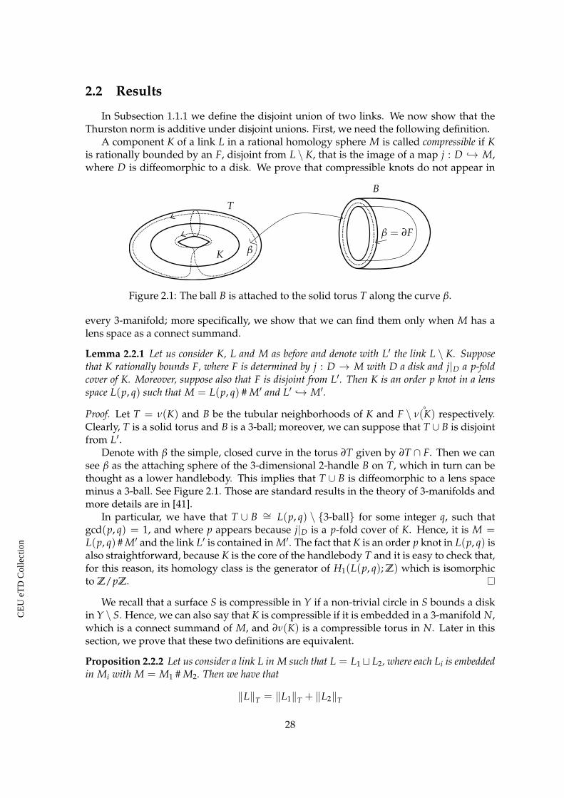
A component K of a link L in a rational homology sphere M is called compressible if Kis rationally bounded by an F, disjoint from L \ K, that is the image of a map j : D ↪→ M,where D is diffeomorphic to a disk. We prove that compressible knots do not appear in
β
β = ∂F
K
T
B
Figure 2.1: The ball B is attached to the solid torus T along the curve β.
every 3-manifold; more specifically, we show that we can find them only when M has alens space as a connect summand.
Lemma 2.2.1 Let us consider K, L and M as before and denote with L′ the link L \ K. Supposethat K rationally bounds F, where F is determined by j : D → M with D a disk and j|D a p-foldcover of K. Moreover, suppose also that F is disjoint from L′. Then K is an order p knot in a lensspace L(p, q) such that M = L(p, q) # M′ and L′ ↪→ M′.
Proof. Let T = ν(K) and B be the tubular neighborhoods of K and F \ ˚ν(K) respectively.Clearly, T is a solid torus and B is a 3-ball; moreover, we can suppose that T ∪ B is disjointfrom L′.
Denote with β the simple, closed curve in the torus ∂T given by ∂T ∩ F. Then we cansee β as the attaching sphere of the 3-dimensional 2-handle B on T, which in turn can bethought as a lower handlebody. This implies that T ∪ B is diffeomorphic to a lens spaceminus a 3-ball. See Figure 2.1. Those are standard results in the theory of 3-manifolds andmore details are in [41].
In particular, we have that T ∪ B ∼= L(p, q) \ {3-ball} for some integer q, such thatgcd(p, q) = 1, and where p appears because j|D is a p-fold cover of K. Hence, it is M =L(p, q) # M′ and the link L′ is contained in M′. The fact that K is an order p knot in L(p, q) isalso straightforward, because K is the core of the handlebody T and it is easy to check that,for this reason, its homology class is the generator of H1(L(p, q); Z) which is isomorphicto Z/pZ.
We recall that a surface S is compressible in Y if a non-trivial circle in S bounds a diskin Y \ S. Hence, we can also say that K is compressible if it is embedded in a 3-manifold N,which is a connect summand of M, and ∂ν(K) is a compressible torus in N. Later in thissection, we prove that these two definitions are equivalent.
Proposition 2.2.2 Let us consider a link L in M such that L = L1 t L2, where each Li is embeddedin Mi with M = M1 # M2. Then we have that
‖L‖T = ‖L1‖T + ‖L2‖T
28
CE
UeT
DC
olle
ctio
n

and the order of L in M is t = lcm(t1, t2), where ti is the order of Li in Mi for i = 1, 2.
Proof. We suppose first that L1 and L2 have no compressible components. Let us consider asurface F which is rationally bounded by L. Fix a separating 2-sphere S ↪→ M, that gives aconnected sum decomposition of M, in a way that S intersects F transversely in a collectionof circles S . Moreover, we suppose that there exist neighborhoods for L1 and L2 which aredisjoint from S, each one lying in one component of M \ S. Take the map j : Σ ↪→ M whichdefines F; if the neighborhoods are chosen small enough then we can also suppose thatthey intersect F only in the image of a neighborhood of ∂Σ.
Now each circle in S separates S into two disks. Let C ⊂ S be a circle that is innermoston F. This means that C bounds a disk D in S, the interior of which misses F. Now use Dto do surgery on F in the following way: create a new surface F from F by deleting a smallannular neighborhood of C and replacing it by two disks, each a “parallel” copy of D, oneon either side of D. We then perform the surgery on F described before on all the circlesin S . At this point F may have closed components, but in this case we just delete them.Therefore, we are left with a disconnected surface whose connected components, that areno longer closed, stay in Mi according wether they bound a component of Li. We call F1the surface given by the union of the components of F of the first type and F2 the other one.
We clearly have that F1 and F2 are disjoint, they lie in M1 and M2 respectively and thatthey do not intersect S; moreover, they are such that
• F1 and F2 have no closed components;
• ML ∩ Fi is a proper submanifold of ML with no disk components, while Fi coincidewith F in a small neighborhood of L for i = 1, 2;
• χ(F1) + χ(F2) = χ(F1 t F2) > χ(F).
Since F is rationally bounded by L and F1 t F2 coincide with F in a neighborhood of L, wehave that Fi has Li as boundary and then [Li] = [0] in the group H∗(M; Q). This impliesthat t is a multiple of both t1 and t2. This proves that t = lcm(t1, t2).
We now want to show that the Thurston norm is additive. The fact that ‖L1 t L2‖T 6‖L1‖T + ‖L2‖T follows immediately from Property 2 in Section 2.1. Then we suppose thatthe inequality is strict: this means that
−χ(F1)
t− χ(F2)
t6 −χ(F)
t< ‖L1‖T + ‖L2‖T .
In particular, at least one of the two surfaces, say F1, is such that −t−1χ(F1) < ‖L1‖T. Thenthe claim follows from the fact that by construction, if t = at1, the class [F1] coincide witha times the class represented by a rational Seifert surface of L1 in H2(ML, ∂ML; Q); whichgives a contradiction.
To conclude we need to prove that, if L is the disjoint union of a link L′ with a compress-ible knot K, it is ‖L‖T = ‖L′‖T + ‖K‖T. This is done in the same way as the previous case,but we take into account the fact that disks do not increase the complexity of a surface.
The proof of this proposition also implies the following corollary.
Corollary 2.2.3 The Thurston norm of a link L in M1 coincides with the one obtained when L isseen as a link in M, where M = M1 # M2. Furthermore, the order of L in M1 concides with theorder of L in M.
29
CE
UeT
DC
olle
ctio
n

In light of Corollary 2.2.3, we use the symbol ‖L‖T not only when L is seen as a linkin M, but also in the case when L lies inside a connect summand of M. Moreover, we cannow prove the following proposition.
Proposition 2.2.4 The component K of a link L in M is compressible if and only if L = K tL′, where K ↪→ N with M = N # M′, and the boundary of the tubular neighborhood of K is acompressible torus in N.
Proof. Let us start to prove the only if implication. It follows easily from the definition ofcompressibility and Corollary 2.2.3 that K rationally bounds F, the image of a disk D underthe map j, in N; where here j is such that j|D is a t-fold cover of K. It remains to show thatt is actually the order of K in N.
We move to the if implication for the moment. In this case we have to show that theknot K is embedded in a connect summand N of M and L′ = L \ K does not intersects N.Then we can conclude by reasoning as in the proof of Proposition 2.2.2.
Knowing this, if we use Lemma 2.2.1 then we immediately prove both the previousclaims. This completes the proof.
We observe that if K is a null-homologous knot then being compressible is equivalentto say that K is an unknot disjoint from L′.
We define the compressibility term of a link L as the rational number
o(L) =o(L)
∑i=1
1ti
,
where o(L) is the number of compressible components in L and t1, ..., to(L) are the orders ofsuch components. Then, in order to prove our main result in Chapter 3 we need anotherlemma.
Lemma 2.2.5 Suppose that L is a non-split link in a rational homology 3-sphere M. Then we havethat
‖L‖T − o(L) = min{−χ(F)
t
},
where F is rationally bounded by L and t is the order of L in M.
Proof. If L is not a compressible knot then o(L) = 0, because otherwise L would be splitfrom Proposition 2.2.4, and so the claim follows from the definition of the Thurston normand Lemma 2.1.3.
On the other hand, if the boundary of a tubular neighborhood of L is a compressibletorus in M then F is rationally bounded by L, where F is the image of a map j : D ↪→ Mwith D diffeomorphic to a disk, and o(L) = t−1. Therefore, its Thurston norm ‖L‖T isequal to zero and the equality in the statement is given by F, since χ(F) = 1.
30
CE
UeT
DC
olle
ctio
n

Chapter 3
Contact structures and Legendrianlinks
3.1 Contact structures
3.1.1 Type of structures and convex surfaces
We recall that a contact structure ξ on an oriented 3-manifold M is a 2-plane field on Msuch that ξ = Ker α, where α is a 1-form on M and α ∧ dα is a volume 3-form for M. Wesay that ξ is cooriented by the form α. Moreover, we call a contact 3-manifold a pair (M, ξ)as before.
We define two relations between contact 3-manifolds. The first has the name of contac-tomorphism and it is given as follows. Consider (M1, ξ1) and (M2, ξ2) as above; they arecontactomorphic if there exists an F : M1 → M2, which is a diffeomorphism and it is suchthat F∗(ξ1) = ξ2.
On the other hand, given a 3-manifold M, we say that (M, ξ1) is contact isotopic to(M, ξ2) if we can find a map F : M× I → M that satisfies the following properties:
• F(·, t) is a contactomorphism for every t ∈ I;
• F(·, 0) = IdM;
• F(·, 1) sends ξ1 into ξ2.
We observe that contactomorphisms give a relation between different contact 3-manifolds,while contact isotopies only relate contact structures on a fixed 3-manifold. Furthermore,the following corollary follows immediately from the previous definitions.
Corollary 3.1.1 Suppose ξ1 and ξ2 are contact isotopic structures on a 3-manifold M. Then(M, ξ1) and (M, ξ2) are contactomorphic.
An embedded disk E, in a contact manifold (M, ξ), is an overtwisted disk if its boundary∂E is such that TE ⊂ ξ and E · eξ = 0, where eξ is the contact framing given by ξ. See [27].In Section 3.2, we see that these conditions are equivalent to say that E is bounded by aLegendrian unknot in M and tbE(∂E) = 0, where tb is called Thurston-Bennequin numberand it is also defined later.
A contact structure ξ on a 3-manifold M is an overtwisted structure if (M, ξ) contains anovertwisted disk. While, we say that ξ is a tight structure if it is not overtwisted.
31
CE
UeT
DC
olle
ctio
n

We now need to recall the definition of convex surface in a contact 3-manifold anddividing set. We use [27] as a reference. We start by saying that a surface S in (M, ξ) iscalled convex if there is a vector field v, transverse to S, whose flow preserves ξ; such avector field is called a contact vector field. We have the following approximation result.
Proposition 3.1.2 Every closed surface Σ can be smoothly perturbed into a convex surface. Fur-thermore, in the case Σ has the link L = L1 ∪ ... ∪ Ln as boundary, if L is such that TL ⊂ ξ andΣ · Li,ξ 6 0 for i = 1, ..., n, where Li,ξ is the contact framing of Li, then Σ can be again smoothlyperturbed into a convex surface, fixing the boundary.
Proof. The closed case is done in [37], while the proof for surfaces with boundary can befound in [50].
If v is a contact vector field in (M, ξ) transverse to S then the set
ΓS = {x ∈ S | v(x) ∈ ξx}
is a collection of embedded curves, and arcs if the surface has non-empty boundary, in Sand is called the dividing set of S in (M, ξ).
We have that the relative homotopy type of ΓS is invariant under contact isotopy. More-over, if the knot K is a component of the boundary of S, and it is Legendrian, which meanssuch that TK ⊂ ξ, then
S · Kξ = −12· |K ∩ ΓS| ,
where Kξ is the contact framing of K. More details can be found in [65].
3.1.2 Classification theorems
In this subsection we briefly state the most important results about existence anduniqueness of tight and overtwisted structures on a given 3-manifold.
Let us start with the overtwisted case. The major theorems in this settings are due toEliashberg [18, 22].
Theorem 3.1.3 (Eliashberg) The homotopy classes of 2-plane fields on an oriented, closed 3-manifold M are in bijection with overtwisted contact structures on M up to isotopy.
This means that every 2-plane field on M is homotopic to an overtwisted contact struc-ture and that two overtwisted structures, which are homotopic as 2-plane fields, are actu-ally contact isotopic. In particular, overtwisted structures exist for every M.
In the specific case of S3, all of the overtwisted structures can be explicitly determined.Let us recall that there is an isomorphism d3 : π3(S2) → Z and a generator of π3(S2) isthe Hopf fibration, introduced in [48]. The map d3 is called the Hopf invariant. Then thefollowing result holds.
Corollary 3.1.4 The space of overtwisted structures on S3 is in bijection with Z and then suchstructures are classified by the Hopf invariant d3.
Proof. From Eliashberg’s Theorem 3.1.3 we have that an overtwisted structure ξ on S3 isdetermined by the homotopy type of ξ as 2-plane field.
Since contact structures are cooriented, there is a vector field v such that v(x) is orthog-onal to ξx for every x ∈ S3 and it is positively oriented. This means that ξ induces a mapfrom S3 to S2 and then its homotopy type is an element of π3(S2).
32
CE
UeT
DC
olle
ctio
n

From now on, we denote the overtwisted structures on S3 with ξn, where d3(ξn) = nand ξ0 is homotopic to the Hopf fibration.
We now suppose that M is non-compact. In this case, an overtwisted contact structureis called tight at infinity if it is tight outside a compact set. Otherwise, we say that it isovertwisted at infinity. We state the version of Theorem 3.1.3 for non-compact 3-manifold.
Theorem 3.1.5 (Eliashberg) The classification of contact structures overtwisted at infinity coin-cides with the homotopical classification of tangent 2-plane distributions.
On the other hand, we do not have a complete classification of tight contact structures,but Ding and Geiges in [16] proved that there exists a prime decomposition under contactconnected sum. We say that a contact manifold (Y, ζ) is prime if (Y, ζ) = (Y1, ζ1) # (Y2, ζ2)implies that at least one of the two summands is contactomorphic to (S3, ξst), which is theunique tight structure on S3 [21].
Theorem 3.1.6 (Ding and Geiges) Every tight contact 3-manifold (M, ξ), that is not (S3, ξst),is contactomorphic to a connected sum
(M1, ξ1) # ... # (Mk, ξk)
of finitely many prime tight contact 3-manifolds. The summands are unique up to order and con-tactomorphism.
More details on the connected sum of contact 3-manifolds can be found in [13].
3.1.3 Fillings
We recall that a smooth 4-manifold is symplectic if it is equipped with a closed non-degenerate differential 2-form ω, called a symplectic form. A contact manifold (M, ξ) iscalled weakly symplectically fillable if there is a compact symplectic 4-manifold (X, ω) suchthat ∂X = M and ω|ξ> 0.
We also say that (M, ξ) is strongly symplectically filled by X if there is a vector field v,transversely pointing out of X along M, such that the Lie derivative Lvω is a positivemultiple of ω in every point and the contraction ιvω is a contact 1-form for ξ.
It is clear from the definition that a strong filling is also a weak filling. Moreover, thetwo notions coincide on rational homology spheres. See [20, 25, 63].
An important result of Eliashberg and Gromov is that simplectically fillable contactstructures are always tight.
Theorem 3.1.7 (Eliashberg and Gromov) Suppose that (M, ξ) is a contact 3-manifold whichadmits a weak symplectic filling. Then the structure ξ is tight.
This theorem was reproved by Ozsváth and Szabó, using Heegaard Floer homology, in[70].
Another type of filling that is interesting to study consists of the family of Stein fillings.A Stein manifold is a triple (X, J, ψ), where J is a complex structure on X, there is a Morsefunction ψ from X to R and ωψ(v, w) = −d(dψ ◦ J)(v, w) is non-degenerate.
A contact manifold (M, ξ) is called Stein fillable if there is a Stein manifold (X, J, ψ) suchthat
• the map ψ is bounded from below;
33
CE
UeT
DC
olle
ctio
n

• the manifold M is a non-critical level of ψ;
• −(dψ ◦ J) is a contact form for ξ.
The following corollary follows easily from the definition of Stein filling.
Corollary 3.1.8 A Stein fillable contact 3-manifold is strongly symplectically fillable
The converse of this result is not true as we know from Ghiggini [36].We can now say a few words on contact surgeries. More details are in [27]. Let K be
a knot in a contact 3-manifold (M, ξ) such that TK ⊂ ξ (a Legendrian knot). It is known,see [35], that K has a neighborhood ν(K) that is contactomorphic to a neighborhood of thex-axis in (R3, Ker (dz− ydx))/ ∼, where ∼ identifies (x, y, z) with (x + 1, y, z).
With respect to these coordinates on ν(K), we can remove ν(K) from M and topologi-cally glue it back by performing a Dehn surgery along K, with framing the contact framing±1. Denote the resulting manifold with M(K,±1). There is a unique way, up to isotopy,to extend ξ|M\ν(K) to a contact structure ξ(K,±1) over all of M(K,±1) so that ξ(K,±1)|ν(K) istight, see [46]. The new contact manifold (M, ξ)(K,±1) is said to be obtained from (M, ξ) by±1-contact surgery along K.
We can iterate this procedure multiple times on different Legendrian knots in M. Thenin this case we say that we are doing a contact surgery on (M, ξ) along a Legendrian link.We recall that every (M, ξ) is obtained from (S3, ξst) by contact surgery [15]. We concludethis subsection with the following theorem.
Theorem 3.1.9 Suppose that a contact manifold (M, ξ) admits a contact surgery presentationwhich contains only −1-surgeries. Then (M, ξ) is Stein fillable.
This fact is proved in [19, 40].
3.2 Legendrian links
A link L in a contact 3-manifold (M, ξ) is called Legendrian if TL ⊂ ξ, which meansthat TpL ⊂ ξp for every p ∈ L.
Two Legendrian links L1 and L2 are Legendrian isotopic if there is a contact isotopy G :M× I → M that sends L1 into L2.
A number or an element of a group is a Legendrian invariant if it remains unchangedunder Legendrian isotopy. In the following thesis, we call classical invariants of Legen-drian links the link type, the Thurston-Bennequin number and the rotation number. Thedefinitions of these invariants, that are given for links in this section, coincide with theones in [2] for knots.
The link type is the most obvious Legendrian invariant. In fact a Legendrian isotopy oflinks is also a smooth isotopy. The second one is the Thurston-Bennequin number, whichwe denote with tb and it is defined as follows. Let us consider a Legendrian link L, withnon-split link type for now, in a rational homology contact 3-sphere (M, ξ). If we call N(L)the normal bundle over L then we have that, since L is Legendrian, N(L) ∩ ξ determines anon-zero vector field v along L, which is uniquely determined after normalization. This isthe definition of the contact framing of L in (M, ξ).
Let Lξ be the link obtained by pushing L along the contact framing. We extract a ratio-nal number from Lξ by saying that
tb(L) = lkQ(L, Lξ) =F · Lξ
t;
34
CE
UeT
DC
olle
ctio
n

where F is a rational Seifert surface for L in M, as defined in Section 2.1, and t is the orderof L in M.
We define the Thurston-Bennequin number of every Legendrian link L by taking tb(L) =tb(L1) + ... + tb(Lr), where the Li’s correspond to the split components of the link type ofL. It follows from the properties of the linking number in Subsection 1.1.1 that tb(L) doesnot depend on the choice of the rational Seifert surface. Moreover, it is also easy to checkthat this number is a Legendrian invariant.
The Thurston-Bennequin number satisfies the properties stated in the following propo-sition.
Proposition 3.2.1 Suppose that L is a Legendrian link in a rational homology contact 3-sphere(M, ξ). Then we have that
1. if L is null-homologous then tb(L) is an integer;
2. if we reverse the orientation of L then tb(−L) = tb(L).
Proof. The link L is null-homologous in M if and only if Li is null-homologous in M forevery i = 1, ..., r, where the Li’s correspond to the split components of the link type asbefore, because of Corollary 2.2.3. Then the first claim follows from Proposition 1.1.2.
Now we observe that −F represents a rational Seifert surface for −L and −Lξ is itscontact framing. Then this clearly means that nothing changes in the definition of tb(−L).
We note that, when M is not a rational homology sphere, the Thurston-Bennequinnumber may depend on the choice of the surface F, even if L is null-homologous; in par-ticular, it depends on the relative homology class of the surface we take. Therefore, in thiscase we define the invariant as
tbΣ(L) = F · Lξ ,
where F is a Seifert surface for L representing the class Σ ∈ H2(M, ML; Z).The third classical invariant of L is the rotation number rot(L). As before, we take M
as a rational homology sphere. Let F be a rational Seifert surface for L. Recall that we havean inclusion j : Σ ↪→ M, which is an embedding on the interior of Σ and an r-fold cover∂Σ → L. Then we can trivialize the pull-back i∗ξ on Σ, because a surface with boundaryretracts on a bouquet of circles.
This means that there exist two sections s1, s2 : Σ → i∗ξ such that {s1(p), s2(p)} is abasis of (i∗ξ)p for every p ∈ ∂Σ. Therefore, if u is the unit vector field tangent to L andoriented coherently, we have that (i∗u)p ∈ (i∗ξ)p, since L is Legendrian, and
(i∗u)p = α(p)s1(p) + β(p)s2(p) for any p ∈ ∂Σ ;
where α and β are real-valued functions.From this we define a map γ in the following way
γ : ∂Σ −→ S1 t ...t S1
p 7−→ (α(p), β(p))|| (α(p), β(p)) ||
and we call rotation number of L the rational number
rot(K) =1t·∑
ideg(γi) ,
35
CE
UeT
DC
olle
ctio
n

where γi is the restriction of γ to the i-th component of ∂Σ and t is the order of L in M. Inthe same way as before, the value of rot L does not depend on the choice of F nor of the si’sand it is a Legendrian invariant.
The following proposition is the version of Proposition 3.2.1 for rot L.
Proposition 3.2.2 Suppose that L is a Legendrian link in a rational homology contact 3-sphere(M, ξ). Then we have that
1. if L is null-homologous then rot(L) is an integer;
2. if we reverse the orientation of L then rot(−L) = − rot(L).
Proof. Property 1 is trivial. In order to prove Property 2, we take −F as rational Seifertsurface and −u as unit tangent vector field, but we can still take s1 and s2 as sections. Thismeans that, if γ′ is the map for −L, it is deg(γ′i) = −deg(γi) for every i.
3.3 Transverse links
A smooth link T ↪→ (M, ξ) is called transverse if TpT ⊕ ξp = Tp M for every p ∈ T andα|T is a volume 1-form for T. This definition implies that transverse links always comewith a natural orientation, induced by ξ.
As for Legendrian links, we say that two transverse links T1 and T2 are transverse isotopicif there is a contact isotopy G : M× I → M that sends T1 into T2.
A Legendrian link L ↪→ (M, ξ) always determines two special transverse links namedpositive and negative transverse push-off of L, that we denote with T+
L and −T−L , where theminus sign appears because transverse links need to be oriented accordingly to the contactstructure.
We briefly recall the construction of T±L . Let Ai = S1 × [−1, 1] be a collection of em-bedded annuli in M such that S1 × {0} = Li and Ai is transverse to ξ for every i = 1, ..., n,where n is the number of components of L. If the Ai’s are sufficiently thin, see [26], thenT±L is the link with components S1× {± 1
2}, which is transverse up to orientation. It is easyto check that any two positive (or negative) transverse push-offs are transversely isotopicand then T±L is uniquely defined, up to transverse isotopy. Moreover, if we reverse theorientation of L then we have that T±−L = −T∓L .
Since we are working with rational homology spheres, we can define the self-linkingnumber sl(T) of a transverse link T with order t in (M, ξ). The self-linking number is oneof the two classical invariants of transverse links, together with the link type. Supposefor now that T is non-split; take a surface F which is rationally bounded by T and themap j : Σ → M that defines F, as described before in Section 2.1. Consider the pull-backbundle j∗ξ on Σ. Then again we have that j∗ξ is trivial. Let v be a non-zero section of j∗ξ.Normalize v so that v|∂Σ defines a link Tξ in ∂ν(T). We define the self-linking number of Tto be
sl(T) =1t· lkQ(T, Tξ) =
F · Tξ
t2 .
This definition coincides with the one given by Baker and Etnyre in [2] for transverse knots.In the case that T has split link smooth type, we consider T1, ..., Tr the connected com-
ponents of T as a smooth link. Then we say that
sl(T) =r
∑i=1
sl(Ti) .
36
CE
UeT
DC
olle
ctio
n

The fact that M is a rational homology sphere tells us that sl(T) is independent of thechoice of the surface F. Furthermore, the self-linking number is a transverse invariant and,as in the Legendrian case, it has the following property.
Corollary 3.3.1 Suppose that T is a null-homologous transverse link in a rational homology con-tact 3-sphere (M, ξ). Then the invariant sl(T) is an integer.
We can find the value of the self-linking number of the transverse push-offs of a Leg-endrian link L, starting from its Thurston-Bennequin and rotation numbers.
Proposition 3.3.2 Let L be an n-component Legendrian link in the rational homology contact3-sphere (M, ξ). Then we have that
sl(T+±L)= tb(L)∓ rot(L) .
Proof. The proof is done in [2] for Legendrian knots. Hence, the claim follows by observingthat
tb(L)∓ rot(L) =n
∑i=1
tb(Li) + 2 ∑i 6=j
lkQ(Li, Lj)∓n
∑i=1
rot(Li) =
=n
∑i=1
sl(T+±Li
) + 2 ∑i 6=j
lkQ(Li, Lj) = sl(T+±L) ,
where the first and the last equality are consequences of Equation (1.1).
3.4 Legendrian and transverse links in (S3, ξst)
3.4.1 Front projections of Legendrian links
In Subsection 1.2.1 we saw that smooth links in S3 can be represented by planar dia-grams; moreover, two such diagrams, corresponding to isotopic links, differ by a sequenceof Reidemeister moves (Figure 1.5). We now describe a similar construction for Legendrianlinks in (S3, ξst).
Since a link in S3 is embedded in R3 and ξst|R3 is still tight, we can work in (R3, ξ),where ξ = Ker(dz− ydx). In fact, there is a unique tight contact structure on R3 up to con-tact isotopy [21]. Hence, we can define the front projection of an n-component Legendrianlink L. This is the map
n⊔i=1
S1 −→ R2
θ 7−→ (x(θ), z(θ))
where θ = (θ1, ..., θn) and (x(θ), y(θ), z(θ)) is the parametrization of L.A generic front projection of L is a special diagram for L with no vertical tangencies,
that are replaced by cusps, and at each crossing, the slope of the overcrossing is smallerthan the one of the undercrossing. An example of front projection is shown in Figure3.1: we picture a diagram of the standard Legendrian unknot O, which is the unique, up toLegendrian isotopy, Legendrian unknot such that tb(O) = −1. This is proved in [24].
There exist moves on Legendrian front projections, called the Legendrian Reidemeistermoves and they are illustrated in Figure 3.2. A further move is the Legendrian planarisotopy; such a move is an isotopy of the front projection that does not introduce verticaltangencies. These moves appear in the following Legendrian analogue of Reidemeister’sTheorem 1.2.1. A proof can be found in [85].
37
CE
UeT
DC
olle
ctio
n

Figure 3.1: A front projection of the standard Legendrian unknot.
Theorem 3.4.1 (Swiatkowski) Two front projections correspond to Legendrian isotopic Legen-drian links if and only if the projections can be connected by Legendrian planar isotopies and byLegendrian Reidemeister moves.
The classical invariants of an oriented Legendrian link L can be easily computed fromits oriented front projection P. We recall that we define the writhe in Subsection 1.1.1. Thenwe have the following formulas:
Type 1 Type 2 Type 3
Figure 3.2: The three Legendrian Reidemeister moves. For each move, we consider allthe possible reflections and orientations, provided that they satisfy the conditions in thedefinition of front projection.
tb(L) = wr(P)− 12· |cusps in P| ; (3.1)
rot(L) =12·(|down-ward cusps in P| − |up-ward cusps in P|
). (3.2)
3.4.2 Braid presentation for transverse links
Transverse links can be studied by using closed braids. We recall that a closed braid isan n-component link in R3, where here we use cylindrical coordinates (r, ψ, z), that can beparametrized by a map
n⊔i=1
S1 −→ R3
θ 7−→ (r(θ), ψ(θ), z(θ))
38
CE
UeT
DC
olle
ctio
n

for which θ = (θ1, ..., θn), r(θ) 6= 0 and ψ′(θ) > 0 for every θ. More details on braids andclosed braids can be found in [5].
To see the connection between braids and transverse links we use the contact structureξsym on R3, which is given by ξsym = Ker
(dz + r2dψ
). Since this structure is contact
isotopic to the standard one, we can transfer any question about ξst to ξsym. Now givena closed braid B, we can isotopy it through closed braid so that it is enough far from thez-axis that the planes that make up ξsym are almost vertical, which means they are close tothe planes spanned by ∂
∂z and ∂∂r . Thus the closed braid type B represents a transverse link.
Bennequin proved the opposite assertion in [4].
Theorem 3.4.2 (Bennequin) Every transverse link in (R3, ξsym) is transversely isotopic to aclosed braid.
Proof. The proof of the theorem follows the same strategy of the one that smooth links canbe braided. See [5]. We just need to check that such procedure can be done in a transverseway. For details we refer to [4, 64].
Let us fix k points pi in a disk D2, for i = 1, ..., k. Then we recall that a k-braid is anembedding of k arcs γi : [0, 1] → D2 × [0, 1] so that γi(t) ∈ D2 × {t} and the endpoints ofthe γi’s, corresponding to 0 (or 1), map as a set to pi in D2× {0} (or D2× {1}). It is easy to
i
i + 1
σi
Figure 3.3: The generator σi for the braid group Bk.
see that braids and closed braids are in one-to-one correspondence.The set of all the k-braids Bk forms a group. Such group is generated by σi for i =
1, ..., k− 1, where σi is as in Figure 3.3. Given a braid b in Bk, then the positive stabilizationof b is bσk in Bk+1. Moreover, a conjugation of b is βbβ−1 for some β ∈ Bk. Then from[64, 91] we have that braid presentations of transversely isotopic links are related by thosetwo moves.
Theorem 3.4.3 (Orevkov and Shevchishin; Wrinkle) Two braids represent the same transverselink if and only if they are related by a finite sequence of positive stabilizations (and their inverse)and conjugations in the braid group.
From [4] we also have that the self-linking number of a transverse link T in (S3, ξst),represented by the closed k-braid B, is computed as follows:
sl(T) = wr(B)− k , (3.3)
where wr(B) is the writhe of B seen as a link diagram for T.
39
CE
UeT
DC
olle
ctio
n

3.5 Connected sum and disjoint union in the contact setting
The definition of connected sum of two 3-manifolds can be easily given also whenthey come together with a contact structure. Let us take two connected contact manifolds(M1, ξ1) and (M2, ξ2); we call M′i (for i = 1, 2) the manifolds obtained from Mi by removingan open Darboux ball, that is a 3-ball with the its unique tight contact structure [21], and wedefine (M1 # M2, ξ1 # ξ2) the contact manifold which is gotten by gluing together M′1 andM′2. The structure ξ1 # ξ2 is well-defined because it is always possible to glue two contactstructures along the boundary of a Darboux ball. Moreover, the result is independent ofthe choice of the balls themselves and we have the following proposition.
Proposition 3.5.1 For every Darboux ball B in the overtwisted manifold (M, ξ) there exists atleast one overtwisted disk disjoint from B. In particular, if (M, ξ) = (M1 # M2, ξ1 # ξ2) and asummand Mi is overtwisted then we can always find overtwisted disks which are contained entirelyin M′i ⊂ M1 # M2.
Proof. From Eliashberg’s classification, the connected sum of (M, ξ) with (S3, ξ0) is alwayscontact isotopic to (M, ξ). Then the first statement can be proved by noting that we canfind two disjoint Darboux balls in (M, ξ) and, since ξ is overtwisted, one can be replacedwith (S3, ξ0) minus a Darboux ball. At this point, the second statement is an immediateconsequence of the first one.
Clearly if (M1, ξ1) is overtwisted then the connected sum is still overtwisted, but if boththe summands are tight then it is important to cite the following result of Colin [13].
Theorem 3.5.2 The connected sum of two contact 3-manifolds (M1 # M2, ξ1 # ξ2) is tight if andonly if (M1, ξ1) and (M2, ξ2) are both tight.
If a sphere S separates a contact manifold (M, ξ) into two components M1 and M2 suchthat smoothly it is M = M1 # M2 then we can ask whether ξ also splits accordingly. Thenwe can state the following lemma.
Lemma 3.5.3 A convex separating sphere S in (M, ξ) gives a connected sum decomposition(M, ξ) = (M1 #S M2, ξ1 #S ξ2) if and only if the dividing set ΓS is trivial, which means thatconsists of a unique simple, closed curve.
Proof. The claim follows from the fact that a contact manifold, whose boundary is a convexsphere, can be glued together with a Darboux ball if and only if its dividing set is trivial asshown in [27].
Etnyre and Honda in [31] extended the definition of connected sum to Legendrianlinks. Suppose that we have two Legendrian links L1 and L2 in (M1, ξ1) and (M2, ξ2)respectively. We take two Darboux balls D1 and D2 as before, but with the condition thatDi ∩ Li is a Legendrian arc αi where αi ∩ ∂Di consists of two points and its front projectionis isotopic to the one in Figure 3.4; we call this the Legendrian elementary tangle. In this way,the link L1 # L2 in (M1 # M2, ξ1 # ξ2) is Legendrian and it does not depend on the choice ofthe Darboux balls Di, but only of which component of Li contains the arc αi.
We observe that we have:
• tb(L1 # L2) = tb(L1) + tb(L2) + 1;
• rot(L1 # L2) = rot(L1) + rot(L2).
40
CE
UeT
DC
olle
ctio
n
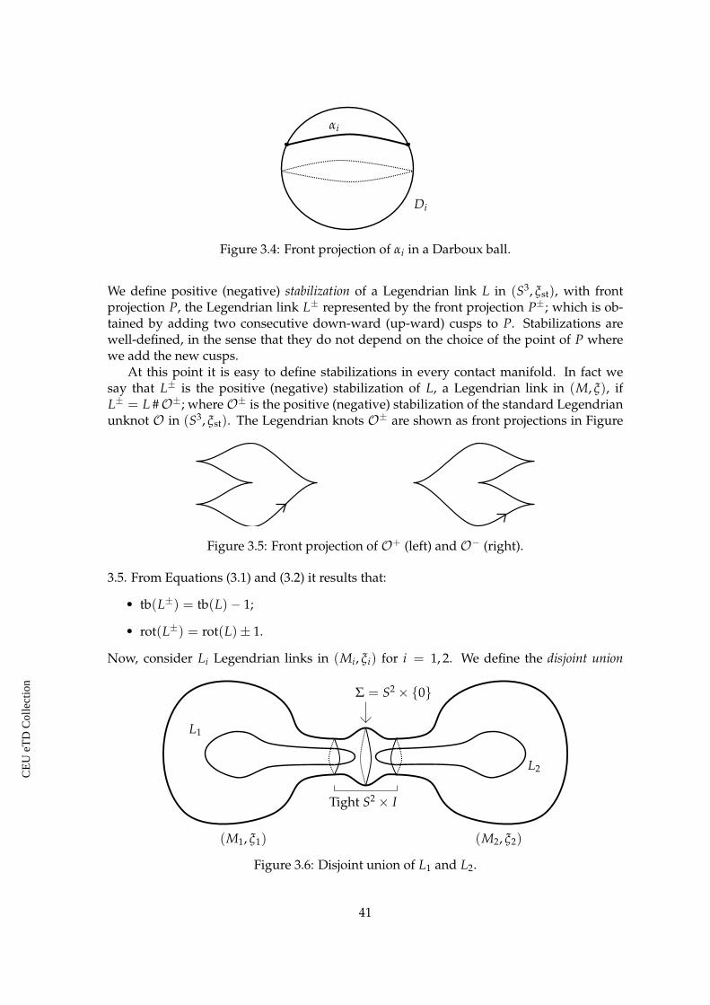
αi
Di
Figure 3.4: Front projection of αi in a Darboux ball.
We define positive (negative) stabilization of a Legendrian link L in (S3, ξst), with frontprojection P, the Legendrian link L± represented by the front projection P±; which is ob-tained by adding two consecutive down-ward (up-ward) cusps to P. Stabilizations arewell-defined, in the sense that they do not depend on the choice of the point of P wherewe add the new cusps.
At this point it is easy to define stabilizations in every contact manifold. In fact wesay that L± is the positive (negative) stabilization of L, a Legendrian link in (M, ξ), ifL± = L #O±; where O± is the positive (negative) stabilization of the standard Legendrianunknot O in (S3, ξst). The Legendrian knots O± are shown as front projections in Figure
Figure 3.5: Front projection of O+ (left) and O− (right).
3.5. From Equations (3.1) and (3.2) it results that:
• tb(L±) = tb(L)− 1;
• rot(L±) = rot(L)± 1.
Now, consider Li Legendrian links in (Mi, ξi) for i = 1, 2. We define the disjoint union
L1
L2
(M1, ξ1) (M2, ξ2)
Σ = S2 × {0}
Tight S2 × I
Figure 3.6: Disjoint union of L1 and L2.
41
CE
UeT
DC
olle
ctio
n

L1 t L2 in (M1 # M2, ξ1 # ξ2) as the Legendrian link given by a particular connected sumL1 #O2 # L2; where O2 is the standard Legendrian unlink with 2 components in (S3, ξst).The connected sum is such that one component of O2 is summed to L1 and the other oneto L2 as shown in Figure 3.6. Note that L1 and L2 are Legendrian links in (M1 # M2, ξ1 # ξ2).
Using the same criterion of the smooth case in Subsection 1.1.1, we say that a Legen-drian link L, in a contact 3-manifold (M, ξ), is split if there exist Li ↪→ (Mi, ξi) for i = 1, 2such that (M, ξ) = (M1, ξ1) # (M2, ξ2) and L is Legendrian isotopic to the disjoint union ofL1 and L2. Otherwise, we say that L is non-split.
Finally, we note that as before:
• tb(L1 t L2) = tb(L1) + tb(L2);
• rot(L1 t L2) = rot(L1) + rot(L2).
3.6 The Thurston-Bennequin inequality
The Thurston-Bennequin inequality is a very powerful result in contact topology. Oneof its most important implications is that, provided the structure is tight, the Thurston-Bennequin numbers of all the Legendrian knots, with the same smooth knot type, arebounded from above. This property actually characterizes tight contact structures on 3-manifolds; in fact, when the structure is overtwisted, it is always possible to increase theThurston-Bennequin number indefinitely, without changing the smooth isotopy class ofthe knot. This is done by connect summing with the boundary of an overtwisted disk.
A proof for a version of the Thurston-Bennequin inequality was given by Eliashberg in[23]. In the following thesis we show that an analogous inequality, involving the Thurstonnorm ‖L‖T of a link defined in Chapter 2, holds for Legendrian and transverse links inevery rational homology contact 3-sphere, equipped with a tight structure. For Legen-drian links in (S3, ξst) this result, and the resulting upper bound for the maximal Thurston-Bennequin number, was found first by Dasbach and Mangum in [14]. On the other hand,if we consider only Legendrian and transverse knots then our bounds coincide with theones of Baker and Etnyre [2].
We recall that if Σ is a surface in (M, ξ) then, at each point x ∈ Σ, we have that lx =ξx ∩ TxΣ is a singular line field on Σ. This line field can be integrated to give a singularfoliation on Σ. This singular foliation is called the characteristic foliation and is denoted withΣξ . More details on foliations are found in [90].
In order to prove our result, we use the same strategy of [2, 23] and then the prooffollows from the following lemma.
Lemma 3.6.1 Suppose that T is a non-split transverse link in a rational homology tight 3-sphere(M, ξ) and take an F in M that is rationally bounded by T. Then we can perturb F in a way thatT′ = F ∩ ∂ν(T) is still transverse and sl(T′) = t · sl(T).
Furthermore, we have thatF · T′ξ 6 −χ(F) ,
where T′ξ is the framing defined as in Section 3.3.
Proof. Consider the map j : Σ→ M which determines F. Let us take a small neighborhoodν(T) of T such that it intersects F only in the image of a neighborhood of ∂Σ, as in theproof of Proposition 2.2.2. Denote the properly embedded surface ML ∩ F with F′, wherethe manifold ML is M \ ˚ν(T).
42
CE
UeT
DC
olle
ctio
n

We know from [2] that we can modify F′ in a way that ∂F′ = T′ is as wanted and thecharacteristic foliation F′ξ is generic. In particular, we can assume that all the singularitiesare isolated elliptic or hyperbolic points. Moreover, each singularity has a sign dependingon whether the orientation of ξ and TF′ agree at the singularity. Let us denote with e± andh± the number of such singularities.
Since we can interpret F′ · Tξ as a relative Euler class, in other words F′ · Tξ is the ob-struction to extending the framing Tξ to a non-zero vector field on F′, we have that
F · T′ξ = F′ · T′ξ = (e− − h−)− (e+ − h+) ,
as in [2]. Moreover, a simple computation gives that
χ(F) = (e+ + e−)− (h+ + h−) ;
thus it isF · T′ξ + χ(F) = 2(e− − h−) . (3.4)
At this point, since ξ is tight, every negative elliptic point is connected to a negative hyper-bolic point, otherwise we could find overtwisted disks in (M, ξ), and then we can cancelthis pair using Giroux’s elimination lemma [38]. This means that we can isotope F′ sothat the characteristic foliation is such that e− = 0 and then the claim follows easily fromEquation (3.4).
We can now prove the main result of the chapter.
Theorem 3.6.2 Suppose that L is a Legendrian link in a tight contact 3-manifold (M, ξ) and M isa rational homology sphere. Then we have that
tb(L) + | rot(L)| 6 ‖L‖T − o(L) .
Furthermore, suppose that T is a transverse link in (M, ξ). Then we have that
sl(T) 6 ‖T‖T − o(T) ,
where the Thurston norm and the compressibility term o are defined in Chapter 2.
Proof. Suppose first that T is a non-split transverse link of order t in (M, ξ). Take an F thatis rationally bounded by T and gives the equality in Lemma 2.2.5. Then from Lemma 3.6.1we have that
sl(T) =sl(T′)
t=
F · T′ξt
6 −χ(F)t
= ‖T‖T − o(T) .
For the second equality we also use that T′ is null-homologous.On the other hand, if T has split smooth link type then we reason as in Section 3.3 and
we write T1, ..., Tr, which are the split components of T. Hence, this time we obtain
sl(T) =r
∑i=1
sl(Ti) 6r
∑i=1‖Ti‖T − o(Ti) = ‖T‖T − o(T) ,
because of Proposition 2.2.2 and the additivity of the Thurston norm and the compressibil-ity term.
Now suppose that L ↪→ (M, ξ) is a Legendrian link. Then from Proposition 3.3.2 wehave that
tb(L)∓ rot(L) = sl(T+±L)6 ‖L‖T − o(L) ;
in fact, L and its transverse push-offs are all smoothly isotopic, up to orientation, and thenthey have same Thurston norm and number of disjoint unknots.
43
CE
UeT
DC
olle
ctio
n

CE
UeT
DC
olle
ctio
n

Chapter 4
Representations of links and3-manifolds
4.1 Heegaard diagrams
4.1.1 3-manifolds and Spinc structures
In this chapter we describe two ways of presenting links in 3-manifolds. Heegaarddiagrams are crucial for the construction of Heegaard Floer homology, both the version formanifolds than the one for links, while in Chapter 6 we use open book decompositions inorder to define some contact and Legendrian invariants.
Hereby, we use terminology from [41, 67, 72]. An oriented handlebody is an oriented3-manifold with boundary obtained by attaching 3-dimensional 1-handles to a 3-ball. It isa classical result on 3-manifolds that any connected, oriented, closed 3-manifold M can bedecomposed, along a separating surface Σ, as the union of two handlebodies [84]. This iscalled a Heegaard decomposition of M.
Let Σ be an oriented, closed, genus g surface, which means a connected sum of g tori,and fix a g-tuple of homologically linearly independent, mutually disjoint curves γ ={γ1, ..., γg}; this is equivalent to say that Σ \ (γ1 ∪ ... ∪ γg) is a connected, planar surface.We call such a collection of curves a system of attaching circles. These curves always specify
α1
β1Σ
Figure 4.1: A Heegaard diagram for the 3-sphere. The torus Σ splits S3 into two solid tori,which are precisely the handlebodies Uα and −Uβ.
a handlebody with boundary Σ, uniquely up to diffeomorphism inducing the identity onthe boundary; moreover, the γi’s bound disjoint, embedded disks Di in the handlebody.
A Heegaard diagram is a triple (Σ, α, β), consisting of an oriented surface Σ equippedwith two systems of attaching circles α = {α1, ..., αg} and β = {β1, ..., βg}, which inter-
45
CE
UeT
DC
olle
ctio
n

sect transversely. The associated 3-manifold M and its Heegaard splitting consist of thehandlebodies Uα and −Uβ, specified by the g-tuples α and β, glued to Σ. See Figure 4.1.
We now define an enriched version of Heegaard diagrams. More specifically, a pointedHeegaard diagram is a quadruple H = (Σ, α, β, w) given by a triple (Σ, α, β) as before and apoint w ∈ Σ \ (α ∪ β).
Now, fix a connected, oriented 3-manifold M, and a generic self-indexing Morse func-tion on M, which has one index zero and one index three critical point. Fix also a generic
α1
α2
α1 + α2
α2
Σ
Figure 4.2: The curve α1 + α2 is the handleslide of α1 over α2.
metric g together with a choice of a gradient flowline, connecting the index zero and threecritical points.
Then, there is an associated pointed Heegaard diagram H for M, whose surface Σ isthe mid-level of the Morse function; the curves in α are the locus of points on Σ where thegradient flowline leaving the index one critical point meets Σ. Similarly, the curves in βare the one which flow from the index two critical point. Finally, w is the point on Σ thatlies on the flowline.
If H is obtained in this manner, from a Morse function f , then we call f a Morse functioncompatible with H. Given a pointed Heegaard diagram for M, it is easy to construct a
αg+1
βg+1
Σg Σg+1
Figure 4.3: The new curves αg+1 and βg+1 are in standard position. This move correspondsto a connected sum with S3.
compatible Morse function f . Moreover, we have the following result.
Theorem 4.1.1 (Ozsváth and Szabó) Any two pointed Heegaard diagrams for M can be con-nected by a finite sequence of the following moves:
1. isotopies and handleslides of the curves in α (or β), supported in the complement of w, seeFigure 4.2;
2. stabilizations (and their inverse), see Figure 4.3.
Proof. The proof is sketched in [72]. The fact that every two (unpointed) Heegaard dia-grams can be connected by such moves follows from standard Morse theory. This can be
46
CE
UeT
DC
olle
ctio
n
done in the complement of a single basepoint because we can trade an isotopy across thebasepoint for a sequence of handleslides in the opposite direction [68].
Using the basepoint we obtain additional information when the 3-manifold is equippedwith a Spinc structure. In this thesis, since we are working on 3-manifolds, the definitionof Spinc structure will be the one given by Turaev in [88]: an isotopy class, away from apoint, of nowhere vanishing vector fields on the manifold.
We define the g-th symmetric power of a genus g surface Σ as the manifold
Symg(Σ) =
g times︷ ︸︸ ︷Σ× ...× Σ
(x1, ..., xg) =(
xσ(1), ..., xσ(g)
)where σ ∈ Sg, the group of permutations of g elements. Consider the g-dimensional tori
Tα = α1 × ...× αg and Tβ = β1 × ...× βg
in Symg(Σ).Given a pointed Heegaard diagram (Σ, α, β, w) for the 3-manifold M, we have a well-
defined mapsw : Tα ∩Tβ −→ Spinc (M)
which sends an intersection point x ∈ Tα ∩ Tβ into the Spinc structure sw(x) on M, asdescribed in [72]. The map is defined as follows. An intersection point x corresponds to ag-tuple of gradient flowlines which connect all the index one and two critical points. Letγx be the union of gradient flowlines passing through each xi ∈ x, and γw be the union ofgradient flowlines passing through each wi ∈ w.
The closure of γx ∪ γw is a collection of arcs whose boundaries consist of all the criticalpoints of f , which is a compatible Morse function. Moreover, each component containsa pair of critical points whose indices have opposite parities. Thus, we can modify thegradient vector field in an arbitrarily small neighborhood of γx ∪ γw to obtain a new vectorfield which vanishes nowhere in M. We call this vector field πw(x) and its homotopy class,in the sense of [88], sw(x).
The space Spinc (M) is (not canonically) identified with H2(M; Z). For this reason wethink of sw(x) as a 2-cohomology class in M.
4.1.2 Links
In the case of links, we need (balanced) multi-pointed Heegaard diagrams. These diagramsare defined as a quintuple (Σ, α, β, w, z), but the objects are slightly different. In fact, nowthe sets α and β consist of g + n− 1 curves, where n > 1 is an integer, and they are suchthat each one spans a g-dimensional subspace of H1(Σ; Z). Moreover, say S1, ..., Sn are theconnected components of Σ \ α and T1, ..., Tn are the ones of Σ \ β, we have that w and z aretwo sets of n basepoints in Σ such that wi, zi ∈ Si ∩ Ti for every i = 1, ..., n. See Figure 4.4.
A multi-pointed Heegaard diagram gives rise to a 3-manifold M together with an ori-ented link L in M as follows. Start from [−1, 1] × Σ and attach 3-dimensional 1-handlesalong copies of the α-curves in {−1} × Σ; then attach three-dimensional 2-handles alongthe copies of the β-curves in {1} × Σ. The result has 2n copies of S2 as boundary, whichwe can close off with 2n 3-handles to get the closed 3-manifold M.
47
CE
UeT
DC
olle
ctio
n

When we connect the basepoints in the components Si and Ti, in the handlebodiesgiven by the α-curves and β-curves, with unknotted and unlinked arcs, we get an embed-ded closed 1-manifold L in M. Next, we orient the link L so that the portions of the link
Σ
L
w1
z1
w2z2
α
β
Figure 4.4: A very simple multi-pointed Heegaard diagram for the 2-component unlink inS3.
in the α-handlebody point away from the w-basepoints and into the z-basepoints. Theresulting link L has n components.
Indeed, any oriented link in any 3-manifold can be presented by an appropriate multi-pointed Heegaard diagram. Given an n-component link, one can find a self-indexingMorse function f : M → R with n index zero and three critical points, and g + n − 1index one and two critical points; with the additional property that there are two n-tuplesof flowlines γw and γz, connecting all the index three and index zero critical points, so thatour link L can be realized as the difference γz − γw. Such a Morse function gives rise to amulti-pointed Heegaard diagram for L in M.
Theorem 4.1.2 (Ozsváth and Szabó) Every two multi-pointed Heegaard diagrams for the samen-component link L in M can be connected by a finite sequence of moves of the following types:
1. isotopies and handleslides of the curves in α (or β ), supported in the complement of w and z;
2. stabilizations (and their inverse).
Proof. The claim follows from Morse theory in the usual manner.
In the previous subsection we saw that, starting from (Σ, α, β, w, z), we define two mapssw and sz from the set of the intersection points Tα ∩Tβ to the one of Spinc structures overM. The relation between these two maps is given in the following proposition.
Proposition 4.1.3 Let (Σ, α, β, w, z) be a multi-pointed Heegaard diagram for a link L in a 3-manifold M. Then we have that
sw(x)− sz(x) = PD[L]
for every x ∈ Tα ∩Tβ.
Proof. It is proved in [68] that sw(x)− sz(x) coincides with the Poincaré dual of [γ], whereγ is a curve in Σ such that αi · γ = 1 for every i = 1, ..., g. The link L respects suchconditions.
As in Section 2.1, let us call ML the 3-manifold with boundary M \ ˚ν(L). When L hasn components we have that ∂ML consists of n disjoint tori. On this kind of 3-manifold we
48
CE
UeT
DC
olle
ctio
n

define a relative Spinc structure as in [72]: the isotopy class, away from a point, of a nowherevanishing vector field such that the restriction on each boundary torus coincides with thecanonical one. This is the vector field induced by the Spin structure on the boundary toriof ML; each structure is given by the product of the extendable Spin structure on the circle(see [72, 88]).
We denote the set of the relative Spinc structures on ML by Spinc (M, L); then we havean identification of Spinc (M, L) with the relative cohomology group H2 (ML, ∂ν(L); Z).Moreover, from [72] we know that, given a multi-pointed Heegaard diagram, we constructa map
sw,z : Tα ∩Tβ −→ Spinc (M, L)
applying the following procedure.Let γ be a gradient flowline connecting an index zero and index three critical point,
and let ν(γ) denote a neighborhood of this flowline. One can construct a nowhere vanish-ing vector field v over ν(γ), which has an integral flowline P which enters ν(γ) from itsboundary, contains γ as a subset and then exits ν(γ).
Let f be an orientation-preserving involution of ν(γ). We can arrange for −v|∂ν(γ) toagree with f ∗(v|∂(ν(γ)∪P). Indeed, we can construct v in the way that the difference v −f ∗(v) is the Poincaré dual of a meridian for γ, thought of as an element of H1(ν(γ) \ P; Z).
Armed with this vector field, we can now define the map sw,z. Fix a Morse function f ,compatible with the Heegaard diagram. Given x ∈ Tα ∩Tβ, consider the flowlines γx, γwand γz. We replace the gradient vector field in a neighborhood of γx so as not to vanishthere. Similarly, we do the same in a neighborhood of γw, using v. In fact, arranging for Pto consist of arcs on γz ∪ γw, we obtain in this manner a vector field on M which containsL as a closed orbit. It is easy to see that this is equivalent to a vector field on ML which is astandard non-vanishing vector field on the boundary tori.
Clearly the relative Spinc structure sw,z(x) extends to the actual Spinc structure sw(x).Furthermore, Poincaré duality gives that
H2 (ML, ∂ν(L); Z) ∼= H1 (ML; Z) ∼= H1 (L; Z)⊕ H1 (M; Z) ∼= Zn ⊕ H2 (M; Z)
and if M is a rational homology sphere then H2 (M; Z) is a finite group. A basis of theimage of H1 (L; Z) ∼= Zn in H1(ML; Z) is given by the homology classes {[µi]}i=1,...,n;where µi is the meridian of the i-th component of L (Figure 1.1). Hence, the isomorphismbetween Spinc (M, L) and H2(ML, ∂ν(L); Z) is given by
sw,z ←→ c1(sw,z)−n
∑i=1
PD[µi] ,
where c1(·) denotes the first Chern class, see [60]. From now on, we think of sw,z as arelative 2-cohomology class under this identification. In particular, when M is a rationalhomology sphere we can write
sw,z(x) =n
∑i=1
ci · PD[µi] + sw(x) for any x ∈ Tα ∩Tβ ,
where ci is an integer for i = 1, ..., n.Let us consider a multi-pointed Heegaard diagram H = (Σ, α, β, w, z), which represents
an n-component link L in a rational homology sphere M. We easily obtain two diagrams
49
CE
UeT
DC
olle
ctio
n

for the link −L, that is gotten from L by reversing the orientation. The first diagram isH1 = (−Σ, β, α, w, z), while the second one is H2 = (Σ, α, β, z, w). Let us denote withs′w,z(x) the relative Spinc structure induced by x in H1 and with sz,w(x) the correspondingone in H2. Then we can prove the following proposition.
Proposition 4.1.4 Let H = (Σ, α, β, w, z) be a multi-pointed Heegaard diagram for L in M asabove. Then we have that
s′w,z(x) = −sw,z(x) and sz,w(x) = sw,z(x)− PD[L]
for every x ∈ Tα ∩Tβ.
Proof. For the first statement, note that if f is a Morse function compatible with H then− f is a Morse function compatible with H1. It is now a straightforward consequence of itsdefinition that if sw,z is represented by v then −v represents sw,z. Thus, the claim follows.
For the second observation, note that the vector fields v and w, representing the non-torsion parts of sw,z(x) and sz,w(x) respectively, differ only in a collar neighborhood of theboundary. In fact, one can see that in this neighborhood, they can be made isotopic awayfrom a neighborhood of the meridian, where they point in opposite directions. in this way,we have proved that
sz,w(x)− sz(x) = sw,z(x)− sw(x)
and then we conclude by applying Proposition 4.1.3.
We briefly recall that we can define an unbalanced multi-pointed Heegaard diagram as amulti-pointed Heegaard diagram (Σ, α, β, w, z) where we drop the condition that both wiand zi are in the intersection between the i-th connected component of Σ \ α and the oneof Σ \ β; instead we only require that there is exactly one element from w and z inside eachcomponent of Σ \ α and Σ \ β. For this kind of diagrams we have that the resulting linkhas at most n components; the other results in this section still apply.
4.2 Open book decompositions
4.2.1 Adapted open book decompositions for links in 3-manifolds
Let us start this section by taking a 3-manifold M. We say that an open book decompositionfor M is a pair (B, π) where
• the binding B is a smooth link in M;
• the map π : M \ B → S1 is a locally trivial fibration such that π−1(θ) = Sθ is acompact surface with ∂Sθ = B for every θ ∈ S1. The surfaces Sθ are called pages ofthe open book.
Moreover, in the case that M comes equipped with a contact structure ξ, we say that thepair (B, π) supports ξ if we can find a 1-form α for ξ such that
• the 2-form dα is a positive area form on each page Sθ ;
• we have α > 0 on the binding B.
50
CE
UeT
DC
olle
ctio
n

Let us consider the page S1 = π−1(1); that is a connected, oriented, compact surface ofgenus g and with l boundary components. Suppose that an n-component Legendrianlink L in (M, ξ) sits inside S1 and its components represent n independent elements inH1(S1; F), where we denote by F the field with two elements. We say that a collection ofdisjoint, simple arcs A = {a1, ..., a2g+l+n−2} is a system of generators for S1 adapted to L if thefollowing conditions hold:
1. the subset A1 t A2 ⊂ A, where A1 = {a1, ..., an} and A2 = {an+1, ..., a2g+l−1}, is abasis of H1(S1, ∂S1; F) ∼= F2g+l−1;
2. we have that L t ai = {1 pt} for every ai ∈ A1 and L ∩ ai = ∅ for i > n. The arcs inthe subset A1 are called distinguished arcs;
3. the subset A3 = {a2g+l , ..., a2g+l+n−2} is such that the surface S1 \ (A2 t A3) has nconnected components; each one containing exactly one component of L.
The arcs in A2 t A3 that appear twice on the same component of the boundary ofS1 \ (A2 t A3) are called dead arcs; the others separating arcs;
4. the elements in A3 are separating arcs such that the disk D = S1 \ (A1 t A2) is dis-connected into n disks and every arc in A3 separates a unique pair of components ofD.
An example of adapted system of generators is shown in Figure 4.5. With this definition in
a1 a2
a3
S1
L
Figure 4.5: A system of generators adapted to the link L.
place, we say that the triple (B, π, A) is an open book decomposition adapted to the Legendrianlink L if
• the pair (B, π) is compatible with M and supports ξ;
• the link L is contained in the page S1;
• the n components of L represent independent elements in H1(S1; Z);
• the set A is a system of generators for S1 adapted to L.
In this case we also say that the adapted open book decomposition (B, π, A) is compatiblewith the triple (L, M, ξ). It is important to observe that, since the components of L arerequired to be independent in homology, we only consider open book decompositionswith pages not diffeomorphic to a disk.
We can prove that open book decompositions adapted to Legendrian links always exist.In order to do this we recall the definition of contact cell decomposition (of a contact 3-manifold) and ribbon of a Legendrian graph. A contact cell decomposition of (M, ξ), see [27],is a finite CW-decomposition of M such that
51
CE
UeT
DC
olle
ctio
n

1. the 1-skeleton is a connected Legendrian graph;
2. each 2-cell E satisfies tb(∂E) = −1;
3. the contact structure ξ is tight when restricted to each 3-cell.
Moreover, if we have a Legendrian link L ↪→ (M, ξ) then we also suppose that
4. the 1-skeleton contains L.
Denote the 1-skeleton of a contact cell decomposition of (M, ξ) with G. Then G is a Legen-drian graph and its ribbon is a compact surface SG satisfying:
• SG retracts onto G;
• TpSG = ξp for every p ∈ G;
• TpSG 6= ξp for every p ∈ S \ G.
We say that an adapted open book decomposition (B, π, A), compatible with the triple(L, M, ξ), comes from a contact cell decomposition if S = π−1(1) is a ribbon of the 1-skeleton of (M, ξ).
Theorem 4.2.1 Every Legendrian link L in a contact 3-manifold (M, ξ) admits an adapted openbook decomposition (B, π, A), which is compatible with the triple (L, M, ξ). Moreover, the contactframing of L coincides with the framing induced on L by the page S1.
Proof. In order to find an open book decomposition (B, π) which comes from a contact celldecomposition of (M, ξ), such that the link L is contained in S1, we simply include the
L
ai
a2g+l
Figure 4.6: We add a new separating arc which is parallel to Li except near the distin-guished arc.
Legendrian link L in the 1-skeleton of the contact cell decomposition. Hence, it results thatthe page S1 is precisely a ribbon of the 1-skeleton of (M, ξ). This argument also gives thatthe two framings of L agree.
The components of L are independent because it is easy to see from the constructionthat there is a collection of disjoint, properly embedded arcs {a1, ..., an} in S1 such that
Li t ai = {1 pt} and Li ∩
⋃j 6=i
aj
= ∅
for every i. To conclude we only need to show that there exists a system of generatorsA = {a1, ..., a2g+l+n−2} for S1 which is adapted to L.
52
CE
UeT
DC
olle
ctio
n

The arcs a1, ..., an are taken as before. If we complete L to a basis of H1(S; F) thenPoincaré-Lefschetz duality gives a basis {a1, ..., a2g+l−1}with the same property. We definea2g+l , ..., a2g+l+n−2 in the following way. Each new separating arc is parallel to Li, extendedby following the distinguished arc to the boundary of S1 as in Figure 4.6. Clearly, it dis-connects the surface, because the first 2g + l − 1 arcs are already a basis of H1(S, ∂S; F). Ifone of the components contains no distinguished arcs, like in Figure 4.7, then we choosethe other endpoint of ai to extend the arc.
In this thesis we use adapted open book decompositions to present Legendrian linksin contact 3-manifolds. Moreover, we study how to relate two different open book decom-
L
ai
a2g+l
Figure 4.7: The picture appears similar to Figure 4.6, but this time the new arc follows thedistinguished arc in the opposite direction.
positions representing isotopic Legendrian links; this is done in Chapter 6.
4.2.2 Abstract open books
An abstract open book is a quintuple (S, Φ,A, z, w) defined as follows. We start with thepair (S, Φ). We have that S = Sg,l is an oriented, connected, compact surface of genus gand with l boundary components, not diffeomorphic to a disk. While Φ is the isotopy classof a diffeomorphism of S into itself which is the identity on ∂S. The class Φ is called themonodromy.
Theorem 4.2.2 (Thurston and Winkelnkemper) The pair (S, Φ) determines a contact 3-manifold.
Proof. We begin by observing that, starting from (S, Φ), we get a 3-manifold MΦ as follows:
MΦ = SΦ ∪ψ
(∏
lS1 × D2
),
where l is the number of boundary components of S and SΦ is the mapping torus of Φ. Bythis we mean
S× [0, 1]�∼ ,
where ∼ is the equivalence relation (φ(x), 0) ∼ (x, 1) for every x ∈ S. Finally, ∪ψ meansthat the diffeomorphism ψ is used to identify the boundaries of the two manifolds.
For each boundary component Si of S, the map ψ : ∂(S1 × D2) → Si × S1 ⊂ SΦ isdefined to be the unique, up to isotopy, diffeomorphism that takes S1 × {p} to Si, wherep ∈ ∂D2, and {q} × ∂D2 to
{q′} × [0, 1]�∼ = S1 ,
53
CE
UeT
DC
olle
ctio
n

where q ∈ S1 and q′ ∈ ∂S.The fact that (S, Φ) also determines a contact structure on MΦ was proved in [87].
The setA consists of two collections of properly embedded arcs, B = {b1, ..., b2g+l+n−2}and C = {c1, ..., c2g+l+n−2} in S with n > 1, such that all the arcs in B are disjoint, all the
bi ci
S
Figure 4.8: Two arcs in strip position.
arcs in C are disjoint and each pair bi, ci appears as in Figure 4.8. We suppose that eachstrip, the grey area between bi and ci, is disjoint from the others. We also want B and C torepresent two systems of generators for the relative homology group H1(S, ∂S; F). In thisway, if we name the strips Ai, we have that S \ ⋃ bi, S \ ⋃ ci and S \ ⋃Ai have exactly nconnected components.
Finally, z and w are two sets of basepoints: w = {w1, ..., wn} and z = {z1, ..., zn}. Werequire these sets to have the following properties:
• there is a zi in each component of S \⋃Ai, with the condition that every componentcontains exactly one element of z;
• each wi is inside one of the strips Ai, between the arcs bi and ci, with the propertythat every strip contains at most one element of w. See Figure 4.9;
b c b c
Si SjSi Sizi zj
wi
zi
wi
Figure 4.9: On the left Si and Sj are different components of S \⋃Ai.
• we choose z and w in a way that each component of S \ B and S \ C contains exactlyone element of z and one element of w.
We can draw an n-component link inside S using the following procedure: we go fromthe z’s to the w’s by crossing B and from w to z by crossing C, as shown in Figure 4.10.Moreover, we observe that the components of the link are independent in S.
Every abstract open book ( f (S), f ◦ Φ ◦ f−1, f (A), f (z), f (w)), obtained from B =(S, Φ,A, z, w) by applying a diffeomorphism f of S into itself, is said to be equivalent toB. Then Theorem 4.2.2 gives the following corollary.
Corollary 4.2.3 Two equivalent pairs (S, φ) and ( f (S), f ◦Φ ◦ f−1) determine contactomorphiccontact 3-manifolds.
54
CE
UeT
DC
olle
ctio
n

b c b c
zw z
w
Figure 4.10: The link is oriented accordingly to the basepoints.
An abstract open book B as above also determines a multi-pointed Heegaard diagram(S ∪ −S, b ∪ b, c ∪ c, z, w) and then a link in a 3-manifold up to (smooth) isotopy. Herethe arcs b and c are defined as h(b) and (h ◦ Φ)(c) respectively, where h : S → −S is theIdentity, seen as an unoriented diffeomorphism. Using this procedure we described wecan prove the following theorem.
Theorem 4.2.4 (Legendrian realization theorem) Every abstract open book (S, Φ,A, z, w) de-termines a Legendrian link L in a contact 3-manifold (M, ξ). Furthermore, equivalent abstractopen books give rise to contactomorphic links.
Proof. The contact manifold (M, ξ) is obtained from the pair (S, Φ) as in Theorem 4.2.2. Itis easy to check that its diffeomorphism type is the same of the manifold obtained from theHeegaard diagram (S ∪−S, b ∪ b, c ∪ c, z, w). This gives us a smooth link L ⊂ S ↪→ M.
The Legendrian realization L is obtained by applying the procedure described in [57]to every component of L. We only need to be careful that the new components are actuallydisjoint.
We are now interested in proving that an adapted open book decomposition (B, π, A)always determines an abstract open book.
Proposition 4.2.5 We can associate to an adapted open book decomposition (B, π, A), compatiblewith the triple (L, M, ξ), an abstact open book (S, Φ,A, z, w) up to isotopy.
Proof. The surface S is obviously the page π−1(1). Now consider the subsets of unit com-plex numbers I± ⊂ S1 ⊂ C with non-negative and non-positive imaginary part. Since theyare contractible, we have that π|π−1(I±) is a trivial bundle. This gives two diffeomorphismsbetween the pages S1 and S−1. The monodromy Φ is precisely the isotopy class of thecomposition of first diffeomorphism with the inverse of the second.
At this point, we want to define the strips A. Hence, we need the collections of arcsB and C: starting from the system of generators A, which is adapted to L ⊂ S, we takethem to be both isotopic to A, in “strip position” like in Figure 4.8 and such that L does notcross the intersections of the arcs in B with the ones in C. We only have an ambiguity on,following the orientation of L, which is the first arc intersected by L. To solve this problemwe have to follow the rule that we fixed in Figure 4.10.
Now we need to fix the basepoints. We put the z’s on L; exactly one on each componentof L \ (L ∩ A). The points in z on different components of L stay in different domainsbecause of Condition 3 in the definition of adapted system of generators. Then S \ A hasn connected components, since the components of L are independent, and each of thesecontains exactly one element of z. Since the z’s are outside of the strips then we have thateach component of S \ B and S \ C also contains only one zi.
The w’s are still put on L, but inside the strips containing the n distinguished arcs. Thepoints w1, ..., wn correspond to A1, ...,An.
55
CE
UeT
DC
olle
ctio
n

CE
UeT
DC
olle
ctio
n

Chapter 5
Heegaard Floer homology
5.1 Link Floer homology
5.1.1 Heegaard diagrams and J-holomorphic curves
Link Floer homology is an invariant for knots and links in 3-manifolds, discovered in2003 by Ozsváth and Szabó [69] and independently by Rasmussen [78], in his PhD thesis.It is constructed, here in the case of rational homology 3-spheres, by associating somechain complexes to a Heegaard diagram, with the help of Lagrangian Floer homology, aconstruction from symplectic geometry given by Andreas Floer in [32]. In this thesis weonly discuss two of these complexes, that we define in this chapter.
Starting from a genus g multi-pointed Heegaard diagram H = (Σ, α, β, w, z) for an n-component link L in M, consider the (g + n − 1)-fold symmetric product of Σ, that wedefined in Subsection 4.1.1, and the (g + n − 1)-dimensional tori Tα and Tβ, which aresubmanifolds of Symg+n−1(Σ).
The surface Σ can be equipped with a complex structure. Then Symg+n−1(Σ) inheritsa complex structure from the direct product of Σ with itself. In particular, this means thatwe can fix an open set of almost-complex structures on Symg+n−1(Σ) compatible with anappropriate symplectic structure, which exists from results in [75].
Consider the set {J(s)}, where s ∈ [0, 1], a path of such almost-complex structures anddefine a J-holomorphic strip, connecting x, y ∈ Tα ∩Tβ, as a continuous map
u : [0, 1]×R −→ Symg+n−1(Σ)
satisfying the following conditions:
1. u maps {0} ×R into Tβ and {1} ×R into Tα;
2. the 1-parameter family of paths ut = u|[0,1]×{t} converges uniformly to the constantpath at x (or y) when t goes to −∞ (or +∞);
3. u satisfies∂u∂s
+ J(s)u(s+it)∂u∂t
= 0 .
Note that the strip [0, 1] ×R is conformally equivalent to the unit disk. This means thatwe can use this notion in place of the one of J-holomorphic disk. Details can be found in[67, 68, 69, 72].
57
CE
UeT
DC
olle
ctio
n

We define the set π2(x, y), where x, y ∈ Tα ∩Tβ, as the set of Z-linear combinations ofthe domains {Dk}, which are the components of Σ \ α ∪ β, such that
a + b = c + d +
(1 if p ∈ x0 otherwise
)+
(−1 if p ∈ y
0 otherwise
);
where a, b, c, d are multiplicities of domains which appear like in Figure 5.1. For everyφ ∈ π2(x, y) we call
nzi(φ) =∣∣φ ∩ {zi} × Symg+n−2(Σ)
∣∣and
nwi(φ) =∣∣φ ∩ {wi} × Symg+n−2(Σ)
∣∣ ;
where here we mean algebraic intersection. Moreover, we say that
nz(φ) =n
∑i=1
nzi(φ) and nw(φ) =n
∑i=1
nwi(φ) .
We also defineM(φ) as the moduli space of holomorphic strips that connects x to y. The
αi
pβi
a
b
c
d
Figure 5.1: Corner point between four domains.
formal dimension ofM(φ), denoted by µ(φ), is the Maslov index; moreover, we call M(φ)the quotientM(φ)/R given by vertical translation of the strip.
For every Spinc structure t on M we define the group cCFL−(H, t) as the free F[U]-module over
Tα ∩Tβ|t={
x ∈ Tα ∩Tβ such that sw(x) = t}
.
Moreover, we obtain another group by taking
CFL(H, t) =cCFL−(H, t)
U = 0;
this group is an F-vector space, where F is again the field with two elements.
5.1.2 Gradings
We can put a bigrading on cCFL−(H, t), where H is a Heeegaard diagram as in theprevious subsection, if we keep the condition that the 3-manifold M is a rational homology3-sphere.
For every x ∈ Tα ∩Tβ|t we denote with (Wx, Jx) an almost-complex 4-manifold, withM as boundary, such that the vector field π(x), induced on M by Jx, is isotopic to the onegiven by x (and w), that we called πw(x) in Subsection 4.1.1. Such 4-manifolds always exist
58
CE
UeT
DC
olle
ctio
n

[60], thus we define the Maslov grading as the absolute Q-grading given by generalizingthe Hopf invariant, defined in Subsection 3.1.2, as follows
M(x) = d3 (M, πw(x)) =14
(c2
1(Wx, Jx)[Wx, ∂Wx]− 3σ(Wx)− 2χ(Wx) + 2)
and we extend it to the whole cCFL−(H, t) by saying that
M(Up) = M(p)− 2 where p ∈ cCFL−(H, t) is homogeneous .
The Maslov grading is independent of the choice of (Wx, Jx).
Lemma 5.1.1 If (W ′x, J′x) is another almost-complex 4-manifold with the same properties of(Wx, Jx) then d3 (M, πw(x)) does not change.
Proof. First, we have that t is torsion, because M is a rational homology sphere. This im-plies that c2
1(Wx, Jx)[Wx, ∂Wx] is well-defined. Now we can find an almost-complex man-ifold (W, J) such that ∂W = −M and the 2-plane field induced by J on −M is isotopic toπw(x). This means that we can glue (W, J) to both our manifolds and obtain two closedalmost-complex 4-manifolds. Since the evaluation on the square of the first Chern class,the signature and the Euler characteristic are all additive under gluing, the Hirzebruch’ssignature theorem gives that
c21(Wx, Jx)[Wx, ∂Wx]− 3σ(Wx)− 2χ(Wx) =
−c21(W, J)[W, ∂W] + 3σ(W) + 2χ(W) =
c21(W
′x, J′x)[W
′x, ∂W ′x]− 3σ(W ′x)− 2χ(W ′x)
and the claim follows.
The difference between the Maslov grading of two intersection points can be expressedeasily.
Proposition 5.1.2 Given φ ∈ π2(x, y) we have that
M(x)−M(y) = µ(φ)− 2nw(φ)
which is an integer.
Proof. From [72] we know that
µ(φ)− µ(ψ) = 2(nw(φ)− nw(ψ))
for every φ, ψ ∈ π2(x, y). Since we can always find ψ such that nw(ψ) = 0, we just applythe Atiyah-Singer index theorem and we obtain that
M(x)−M(y) = µ(ψ) = µ(φ)− 2nw(φ) .
The Maslov grading gives an F-splitting
cCFL−(H, t) =⊕d∈Q
cCFL−d (H, t) ;
59
CE
UeT
DC
olle
ctio
n

moreover, the same holds for CFL(H, t).The definition of M(x) does not require that there is a link L → M. The grading that
we are going to define now, on the other hand, strictly requires that we take L, which hasn components, into account. We call the Alexander multi-grading of x ∈ Tα ∩ Tβ|t as then-tuple (s1, ..., sn) such that
sw,z(x) =n
∑i=1
2si · PD[µi] + sw(x) .
Since L always admits a rational Seifert surface F, see Section 2.1, if t is the order of thelink in M then we define the Alexander absolute Z
2t -grading as follows:
A(x) =n
∑i=1
si =sw,z(x)[F]
2t
and we extend it on the whole cCFL−(H, t) by saying that
A(Up) = A(p)− 1 where p ∈ cCFL−(H, t) is homogeneous .
The Alexander grading is independent of the choice of the surface F.
Lemma 5.1.3 If F′ is another rational Seifert surface for L then the value of A(x) does not change.
Proof. The gluing F ∪ −F′ defines a closed surface and then a 2-homology class in ML =
M \ ˚ν(L) and M. Since H2 (M; Z) is trivial, then [F ∪−F′] is null-homologous in it andalso in H2 (ML; Z). This means that
0 = sw,z(x)[F ∪−F′
]= sw,z(x)[F]− sw,z(x)
[F′]
.
Like for the Maslov grading, we can compute the difference between the Alexandergrading of two intersection points.
Proposition 5.1.4 Given φ ∈ π2(x, y) we have that
A(x)− A(y) = nz(φ)− nw(φ)
which is again an integer.
Proof. From [72] we know that
sw,z(x)− sw,z(y) = 2 ·n
∑i=1
(nzi(φ)− nwi(φ)
)· PD[µi] .
Then the claim follows by evaluating both sides of this equation with [F], where F is arational Seifert surface for L.
We have another F-splitting
cCFL−(H, t) =⊕
d,s∈Q
cCFL−d,s(H, t)
and then again the same is true for CFL(H, t).
60
CE
UeT
DC
olle
ctio
n

5.1.3 Differential
In the previous subsection we introduced the underlying space of our chain complexes;now we want to construct the differentials. We define ∂− in the following way
∂−x = ∑y∈Tα∩Tβ|t
∑φ∈π2(x,y),
µ(φ)=1,nz(φ)=0
∣∣∣M(φ)∣∣∣ ·Unw(φ)y
and∂−(Ux) = U · ∂−x
for every x ∈ Tα ∩Tβ|t.We note that, since we are interested in φ’s that are image of some J-holomorphic disks,
we have that nzi(φ), nwi(φ) > 0 [68]. This means that nz(φ) = nw(φ) = 0 if and only ifnzi(φ) = nwi(φ) = 0 for every i = 1, ..., n.
The map ∂− is well-defined if the diagram D is admissible, which means that everyφ ∈ π2(x, x) with nw(φ) = 0, representing a non-trivial homology class, has both positiveand negative local multiplicities.
Lemma 5.1.5 If M is a rational homology 3-sphere then, given a multi-pointed Heegaard diagram(Σ, α, β, w, z), we can always achieve admissibility through isotopies.
Proof. The proof is taken from [72]. We embed in Σ a tree Γ, whose n vertices are thebasepoints in w. We claim that admissibility can be achieved by isotoping some of theβ-curves in a regular neighborhood of Γ. More specifically, if γ is an arc connecting w1 tow2 in Γ then we perform an isotopy of the β’s in a regular neighborhood of γ, in such amanner that there is a pair of arcs δ1 and δ2 so that δ1 ∪ δ2 is isotopic to γ as an arc from w1to w2, but δ1 is disjoint from the β-circles, while δ2 is disjoint from the α-circles.
Moreover, we find another pair of arcs δ′1 and δ′2 so that δ′1 ∪ δ′2 is isotopic to γ, only thistime δ′1 is disjoint from the α-circles, while δ′2 is disjoint from the β-circles. Isotoping the β’sin a regular neighborhood of all the edges in Γ as above, we obtain a Heegaard diagramthat we claim is weakly admissible.
Suppose that φ ∈ π2(x, x), which decomposes as φ = A + B where A has boundary onTα and B has boundary on Tβ, has the property that the oriented intersection number of∂A with γ is non-zero. Then, at the intermediate endpoint of δ1, we see that A+ B has localmultiplicity given by ∂A ∩ γ, while at the intermediate endpoint of δ′1 we have that A + Bhas local multiplicity given by ∂B∩ γ = −∂A∩ γ, since φ ∈ π2(x, x) [68]. Thus, if for someedge in Γ it is ∂A ∩ γ 6= 0, then φ = A + B has both positive and negative coefficients.
However, if φ = A + B as above and ∂A has algebraic intersection number equal tozero with each edge in Γ then, after subtracting off nw1(A) of copies of Σ, we can write φ =A′ + B′, where A′ and B′ again have boundaries on Tα and Tβ and nwi(A) = nwi(B) = 0.Hence, a simple computation gives that φ = 0.
We now prove that ∂− ◦ ∂− = 0. See [72] for more details.
Theorem 5.1.6 (Ozsváth and Szabó) We have that ∂−(∂−x) is zero for every x ∈ Tα ∩Tβ|t andevery Spinc structure t on M, which means that ∂− is a differential.
Proof. We consider the moduli space M(φ), where φ ∈ π2(x, z) is non-negative withµ(φ) = 2, x and z are intersection points and nz(φ) = 0. We use a structure theorem
61
CE
UeT
DC
olle
ctio
n

in [33, 69] which proves that there is a compact 1-dimensional manifold with boundary,whose interior is M(φ), and its boundary is identified with⋃
y
⋃φ1∈π2(x,y),φ2∈π2(y,z)
µ(φ1)=µ(φ2)=1,φ1∗φ2=φnz(φ1)=nz(φ2)=0
M(φ1)× M(φ2) .
Since a compact 1-manifold has an even number of boundary points, we can conclude that
∑y
∑φ1∈π2(x,y),φ2∈π2(y,z)
µ(φ1)=µ(φ2)=1,φ1∗φ2=φnz(φ1)=nz(φ2)=0
∣∣∣M(φ1)∣∣∣ · ∣∣∣M(φ2)
∣∣∣ ·Unw(φ) = 0 .
Adding up the left-hand-side over all φ ∈ π2(x, z) with µ(φ) = 2 computes the z compo-nent of ∂−(∂−x), then ∂− ◦ ∂− = 0.
Using Lemma 5.1.5 and Theorem 5.1.6, we obtain the chain complexes(cCFL−(H, t), ∂−
)and
(CFL(H, t), ∂ = ∂−|U=0
).
Moreover, Proposition 5.1.2 leads to the following result.
Proposition 5.1.7 For every intersection point x ∈ Tα ∩Tβ|t the element ∂−x is homogeneouswith respect to the Maslov grading and M(∂−x) = M(x)− 1.
Proof. If Unw(φ)y, where φ ∈ π2(x, y) and y ∈ Tα ∩ Tβ|t, is a monomial of ∂−x then wehave that
M(
Unw(φ)y)= M(y)− 2nw(φ) = M(x)− µ(φ) = M(x)− 1 .
The last equality holds because in the differential we only consider φ’s with Maslov indexequal to 1.
This implies that∂−d : cCFL−d (H, t) −→ cCFL−d−1(H, t)
is the restriction of the differential to cCFL−d (H, t).In the same way, Proposition 5.1.4 immediately gives a similar relation for the Alexan-
der grading.
Proposition 5.1.8 For every intersection point x ∈ Tα ∩Tβ|t the element ∂−x is homogeneouswith respect to the Alexander grading and A(∂−x) = A(x).
Proof. If Unw(φ)y, where φ ∈ π2(x, y) and y ∈ Tα ∩ Tβ|t, is a monomial of ∂−x then wehave that
A(
Unw(φ)y)= A(y)− nw(φ) = A(x)− nz(φ) = A(x) .
The last equality holds because in the differential we only consider φ’s with nz(φ) = 0.
Hence, the map∂−d,s : cCFL−d,s(H, t) −→ cCFL−d−1,s(H, t)
is the restriction of the differential to cCFL−d,s(H, t).
62
CE
UeT
DC
olle
ctio
n

5.1.4 Homology
In this section we define two versions of link Floer homology, corresponding to thechain complexes that we defined in the previous subsection. The first group is called col-lapsed link Floer homology and it is defined by
cHFL−(H, t) =⊕
d,s∈Q
cHFL−d,s(H, t) ,
where
cHFL−d,s(H, t) =Ker ∂−d,s
Im ∂−d+1,s.
The group cHFL−(H, t) is a bigraded F-vector space with a structure of finite dimensionalF[U]-module.
Theorem 5.1.9 (Ozsváth and Szabó) The isomorphism type of the group cHFL−(H, t) is invari-ant under smooth isotopy of the link L ↪→ M. Which means that, if H′ is another multi-pointedHeegaard diagram for a link isotopic to L in M, it is
cHFL−d,s(H, t) ∼=F cHFL−d,s(H′, t)
for every d, s ∈ Q and t ∈ Spinc (M).
Hence, we can denote cHFL−(H, t) with cHFL− (M, L, t). We leave the proof of thistheorem for Section 5.3.
The second version that we want to study is the hat link Floer homology group
HFL(H, t) =⊕
d,s∈Q
HFLd,s(H, t) ;
given by
HFLd,s(H, t) =Ker ∂d,s
Im ∂d+1,s.
The group HFL(H, t) is a finite dimensional, bigraded F-vector space. Moreover, as thecollapsed minus version, it is also a smooth isotopy invariant of links in 3-manifolds. Infact, we have an analogous theorem in this case.
Theorem 5.1.10 (Ozsváth and Szabó) The isomorphism type of the group HFL(H, t) is invari-ant under smooth isotopy of the link L ↪→ M. Which means that, if H′ is another multi-pointedHeegaard diagram for a link isotopic to L in M, it is
HFLd,s(H, t) ∼=F HFLd,s(H′, t)
for every d, s ∈ Q and t ∈ Spinc (M).
Hence, we can denote HFL(H, t) with HFL (M, L, t). Theorems 5.1.9 and 5.1.10 havebeen proved in [69] for knots and generalized to links in [72].
The group HFL has the following interesting symmetry property.
63
CE
UeT
DC
olle
ctio
n
Proposition 5.1.11 Given a smooth link L in a rational homology 3-sphere M, we have that
HFLd,s (M, L, t) ∼=F HFLd−2s,−s (M, L,−t+ PD[L])
for every d, s ∈ Q and t ∈ Spinc (M).
Proof. It follows from the relation between the two relative Spinc structures obtainedby reversing the orientation of L, see Subsection 4.1.2 before. More specifically, given(Σ, α, β, w, z) a multi-pointed Heegaard diagram for L in M, we call H1 = (Σ, β, α, w, z)the first diagram for −L. Then Proposition 4.1.4 gives us the isomorphism
Φ1 : HFLd,s (M, L, t) −→ HFLd,s (M,−L,−t) .
In the same way, we call H2 = (Σ, α, β, z, w), which also represents the link −L. Now fromPropositions 4.1.3 and 4.1.4 we obtain the map
Φ2 : HFLd,s (M,−L,−t) −→ HFLd−2s,−s (M, L,−t+ PD[L])
and the proof is completed by taking the composition of Φ1 and Φ2.
We can use this property to normalize the relative grading a(x, y) = nz(φ) − nw(φ),where φ ∈ π2(x, y), given in Proposition 5.1.4. Hence, this can be seen as an equivalentdefinition of the Alexander grading; in fact, we have that A(x) is the only normalizationof a(x, y) which respects the symmetry in Proposition 5.1.11. This property proves thefollowing corollary.
Corollary 5.1.12 For every multi-pointed Heegaard diagram (Σ, α, β, w, z), and x ∈ Tα ∩Tβ, wehave that
2A(x) = M(x)−Mz(x) ,
where A(x) and M(x) are the Alexander and Maslov grading of x and Mz(x) = d3 (M, πz(x)).
Proof. From Propositions 5.1.2 and 5.1.4 we have that the relative grading
b(x, y) = (M(x)−M(y))− (Mz(x)−Mz(y))
coincides with 2a(x, y) = 2(A(x) − A(y)). Therefore, we just need to show that b(x, y)satisfies the symmetries in Proposition 5.1.11 and this can be done easily.
5.2 Heegaard Floer homology of 3-manifolds
Let us take a multi-pointed Heegaard diagram H = (Σ, α, β, w), where the set w con-tains n basepoints. We can change the differential ∂ to ∂w as follows:
∂wx = ∑y∈Tα∩Tβ|t
∑φ∈π2(x,y),
µ(φ)=1,nw(φ)=0
∣∣∣M(φ)∣∣∣ · y
for every x ∈ Tα ∩Tβ|t and ∂w is U-equivariant. The new complex(
CF(H, t), ∂w
)is well-
defined. Moreover, its homology
HF(H, t) =⊕d∈Q
HFd(H, t)
is an invariant of the manifold, once we fix the number of basepoints in H, as stated in thefollowing theorem.
64
CE
UeT
DC
olle
ctio
n
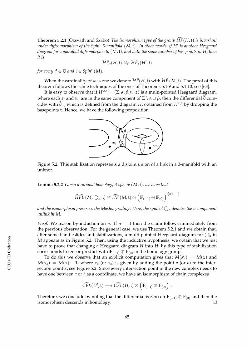
Theorem 5.2.1 (Ozsváth and Szabó) The isomorphism type of the group HF(H, t) is invariantunder diffeomorphism of the Spinc 3-manifold (M, t). In other words, if H′ is another Heegaarddiagram for a manifold diffeomorphic to (M, t), and with the same number of basepoints in H, thenit is
HFd(H, t) ∼=F HFd(H′, t)
for every d ∈ Q and t ∈ Spinc (M).
When the cardinality of w is one we denote HF(H, t) with HF (M, t). The proof of thistheorem follows the same techniques of the ones of Theorems 5.1.9 and 5.1.10, see [68].
It is easy to observe that if Hw,z = (Σ, α, β, w, z) is a multi-pointed Heegaard diagram,where each zi and wi are in the same component of Σ \ α ∪ β, then the differential ∂ coin-cides with ∂w, which is defined from the diagram H, obtained from Hw,z by dropping thebasepoints z. Hence, we have the following proposition.
b a
w1 wn
Figure 5.2: This stabilization represents a disjoint union of a link in a 3-manifold with anunknot.
Lemma 5.2.2 Given a rational homology 3-sphere (M, t), we have that
HFL (M,©n, t) ∼= HF (M, t)⊗(
F(−1) ⊕F(0)
)⊗(n−1)
and the isomorphism preserves the Maslov grading. Here, the symbol©n denotes the n componentunlink in M.
Proof. We reason by induction on n. If n = 1 then the claim follows immediately fromthe previous observation. For the general case, we use Theorem 5.2.1 and we obtain that,after some handleslides and stabilizations, a multi-pointed Heegaard diagram for ©n inM appears as in Figure 5.2. Then, using the inductive hypothesis, we obtain that we justhave to prove that changing a Heegaard diagram H into H′ by this type of stabilizationcorresponds to tensor product with F(−1) ⊕F(0) in the homology group.
To do this we observe that an explicit computation gives that M(xa) = M(x) andM(xb) = M(x) − 1, where xa (or xb) is given by adding the point a (or b) to the inter-section point x; see Figure 5.2. Since every intersection point in the new complex needs tohave one between a or b as a coordinate, we have an isomorphism of chain complexes
CFL(H′, t) −→ CFL(H, t)⊗(
F(−1) ⊕F(0)
).
Therefore, we conclude by noting that the differential is zero on F(−1) ⊕ F(0) and then theisomorphism descends in homology.
65
CE
UeT
DC
olle
ctio
n

This lemma implies the following theorem.
Theorem 5.2.3 (Ozsváth and Szabó) If the set w in the Heegaard diagram H contains n base-points then we have that
HF(H, t) ∼=F HF (M, t)⊗(
F(−1) ⊕F(0)
)⊗(n−1). (5.1)
More explicitly, it is
HFd(H, t) ∼=F
n−1⊕i=0
(n− 1
i
)HFd+i (M, t)
for every d ∈ Q and t ∈ Spinc (M).
From Propositions 5.1.4 and 5.1.11 we see that the Alexander grading is always zero inthe case of unlinks. Hence, we can express the hat link Floer homology of©n entirely interms of the homology of M:
HFLd,s (M,©n, t) ∼=
n−1⊕i=0
(n− 1
i
)HFd+i (M, t) if s = 0
{0} otherwise
.
A particular case is given by the 2-component unlink ©2 in S3. In fact, we have thatHFL (©2) ∼= F(−1,0) ⊕ F(0,0); note that we do not specify the manifold when we work inthe 3-sphere.
We conclude this section by computing the homology of the unlink also in the col-lapsed version. We observe that, for the same argument used to prove Lemma 5.2.2, thedifferential ∂− coincides with ∂ too if we choose an appropriate diagram. Moreover, thegenerators of cCFL−(H, t) and CF(H, t) are the same; with the difference that the firstspace is an F[U]-module. This gives the following result.
Corollary 5.2.4 The homology group cHFL− (M,©n, t), seen as an F[U]-module, is the tensorproduct of HFL (M,©n, t) with (the module) F[U] over F.
Using Lemma 5.2.2 we can restate this corollary by saying that
cHFL−d,s (M,©n, t) ∼=
n−1⊕i=0
(n− 1
i
)HFd−2s+i (M, t) if s 6 0
{0} otherwise
.
5.3 Invariance
5.3.1 Choice of the almost-complex structures
In this section we give ideas for the proofs that link Floer homology is invariant underthe moves in Section 4.1, that relates two multi-pointed Heegaard diagrams represent-ing the same link L in the Spinc 3-manifold (M, t), and the analytic input of the path of
66
CE
UeT
DC
olle
ctio
n

almost-complex structures J(s) on the symmetric power and the complex structure on Σ,see Subsection 5.1.1. We always suppose that M is a rational homology 3-sphere.
Suppose that H = (Σ, α, β, w, z) is a multi-pointed Heegaard diagram for an n-component link in M. First, we argue that if we fix a complex structure on Σ then the linkFloer homology groups are independent of the choice of J(s) on Symg+n−1(Σ). Take twopaths J0(s) and J1(s) on Symg+n−1(Σ); since the symmetric power is simply-connected, wecan connect J0(s) and J1(s) with a 2-parameter family J : [0, 1] × [0, 1] → Symg+n−1(Σ),thought of as a 1-parameter family of paths indexed by t ∈ [0, 1] where Jt(s) is the pathobtained by fixing t. In fact, we can arrange that Jt(s) is independent of t for t’s near tozero or one, so that Jt(s) can be naturally extended to the whole R.
Then, as it is familiar in Floer theory, we can define an associated chain map
Φ−Jt(s):(
cCFL−(H, t), ∂−J0(s)
)−→
(cCFL−(H, t), ∂−J1(s)
)by
Φ−Jt(s)x = ∑
y∑
φ∈π2(x,y)µ(φ)=1,nz(φ)=0
∣∣∣MJt(s)(φ)∣∣∣ ·Unw(φ)y ,
where MJt(s)(φ) denotes the moduli space of holomorphic strips with a time-dependentcomplex structure on the target.
The usual arguments from Floer theory then apply to show that Φ−Jt(s)is a chain map
which induces an isomorphism in homology. We give a sketch of the proof of this fact. Thedetails can be found in [68].
A transversality theorem in [68] shows that, for a generic path Jt(s), the zero-dimensional components of the moduli spaces MJt(s)(φ) are smoothly cut out and com-pact. Thus, the map Φ−Jt(s)
is well-defined. To show that it is a chain map, we consider
the ends of the 1-dimensional moduli spaces MJt(s)(ψ), where µ(ψ) = 2. Then the sameargument in the proof of Theorem 5.1.6 and Gromov’s compactness [42] give that Φ−Jt(s)
isalso a chain map.
The fact that Φ−Jt(s)induces an isomorphism in homology is done by showing that the
composition with Φ−J1−t(s)is chain homotopic to the identity; we recall that we said what
is a chain homotopy in Subsection 1.4.2. The chain homotopy is constructed by using ahomotopy Jt,τ(s) between two 2-parameter families of complex structures. We can definea moduli space
MJt,τ(s)(φ) =⋃
η∈[0,1]
MJt,η(s)
for each φ ∈ π2(x, y). For a generic Jt,τ(s) this manifold has dimension µ(φ) + 1. We definea map
H−Jt,τ(s)x = ∑
y∑
φ∈π2(x,y)µ(φ)=0,nz(φ)=0
∣∣∣MJt,τ(s)(φ)∣∣∣ ·Unw(φ)y .
To see then that H−Jt,τ(s)is the chain homotopy between Φ−Jt(s)
◦Φ−J1−t(s)and the identity map,
we reason in the same way as before [68].Next, we see that the chain complex is independent of the complex structure J on the
surface Σ. To this end, we observe that the chain complexes remain unchanged under
67
CE
UeT
DC
olle
ctio
n

small perturbations of the path of almost-complex structures J(s). Furthermore, we canapproximate J(s) with a symmetric path J′(s), induced by a complex structure J′ close toJ. This shows that the Floer homology is also independent of the choice of J, since thespace of allowed complex structures over Σ is connected, because it is obtained from thespace of all complex structures by removing a codimension two subset, see [68].
5.3.2 Isotopies
Consider two multi-pointed Heegaard diagram H = (Σ, α, β, w, z) and H′ =(Σ, α′, β′, w, z) which differ by an isotopy. First of all, isotopies which preserve the con-dition that the α are transverse to the β can be thought of as variations in the metric, orequivalently the complex structure on Σ. Hence, the invariance of the Floer homologyunder such isotopies follows from Subsection 5.3.1.
It suffices then to show that the homology remains unchanged when a pair of cancelingintersection points between, α1 and β1 is introduced. See Figure 5.3 for an illustration.Such an isotopy can be realized by moving α by an exact Hamiltonian diffeomorphism ofΣ. We recall that, on a symplectic manifold, a 1-parameter family of real-valued functionsHt naturally gives rise to a unique 1-parameter family of Hamiltonian vector fields Xt,specified by
ω(Xt, ·) = dHt ,
where the left-hand side denotes the contraction of the symplectic form ω with the vectorfield. A 1-parameter family of diffeomorphisms Ψt is said to be an exact Hamiltonian isotopyif it is obtained by integrating a Hamiltonian vector field, which means when
• Ψ0 is the Identity;
•dΨt
dt= Xt.
By taking a positive bump function h, supported in a neighborhood of a point which lieson α1, and letting f : R→ [0, 1] be a non-negative smooth function whose support is (0, 1),we can consider the Hamiltonian Ht = f (t)h. The corresponding diffeomorphism movesthe curve α1 slightly, without moving any of the other curves in α.
β1
α1
α′1
β1H
H′
Figure 5.3: By moving the curve α1 to α′1 through a Hamiltonian isotopy, we introduce apair of canceling intersection points.
We assume that the exact Hamiltonian is supported on Σ \ (α2 ∪ ... ∪ αg+n−1 ∪ w ∪ z)and that the Hamiltonian is supported in [0, 1]. The isotopy Ψt induces an isotopy of Tα.We need to show that this isotopy gives a map on Floer homology, by imitating the usualconstructions from Lagrangian Floer theory.
The map is induced by counting points in the zero-dimensional components of themoduli spaces with a time-dependent constraint. To be precise, here, we fix a 1-parameterfamily J(s) of almost-complex structures on the symmetric power of Σ. Now, we have
68
CE
UeT
DC
olle
ctio
n

homotopy classes of holomorphic strips πΨt2 (x, y), where x is an intersection point and
y ∈ Ψ1(Tα) ∩ Tβ, which denote homotopy classes of maps satisfying the condition inSubsection 5.1.1 and such that
u(1 + it) ∈ Ψ1(Tα) and u(0 + it) ∈ Tβ
for every t ∈ [0, 1].Now, we define the map associated to the isotopy
Γ−Ψt: cCFL−(H) −→ cCFL−(H′)
by the formulaΓ−Ψt
x = ∑y
∑φ∈π
Ψt2 (x,y)
µ(φ)=1,nz(φ)=0
∣∣∣MΨt(φ)∣∣∣ ·Unw(φ)y .
The important observation is that the moduli spaces considered have Gromov compactifi-cations. This is shown in [68]. Then, the fact that Γ−Ψt
induces an isomorphism in homologycan be proved in the same way as in Subsection 5.3.1.
5.3.3 Handleslides
Consider a multi-pointed Heegaard diagram H′ = (Σ, α, γ, w, z) which is obtainedfrom (Σ, α, β, w, z) by a single handleslide on a curve in β. Then there is a chain map
Ψαβγ : cCFL−(H, t) −→ cCFL−(H, t′)
defined by counting holomorphic triangles as follows
Ψαβγx = ∑y
∑φ∈π2(x,Θβγ,y)
µ(φ)=1,nz(φ)=0
∣∣∣M(φ)∣∣∣ ·Unw(φ)y ,
where Θβγ is the canonical top-generator of the homology of the chain complex(CF−(Σ, β, γ, w), ∂−w
), whose definition is in [72] together with all the details.
Let us denote with Ψ∗αβγ the induced map in homology, then we note that
sw,z(x) = s′w,z
(Ψ∗αβγ(x)
),
where here s′w,z is the map associated to the Heegaard diagram H′, since the triangles usedin the definition of Ψ∗ are disjoint from w and z.
Now, associativity of the triangle maps [72] gives that the map (Ψαγβ′ ◦ Ψαβγ)∗ is an
isomorphism, where
Ψαγβ′(Ψαβγ(x)) = ∑y
∑φ∈π2(x,Θββ′ ,y)
µ(φ)=1,nz(φ)=0
∣∣∣M(φ)∣∣∣ ·Unw(φ)y
and β′ is a small perturbation of β such that each β′i intersects βi in precisely two intersec-tion points. Therefore, we have that the map Ψ∗αβγ is also an isomorphism.
69
CE
UeT
DC
olle
ctio
n
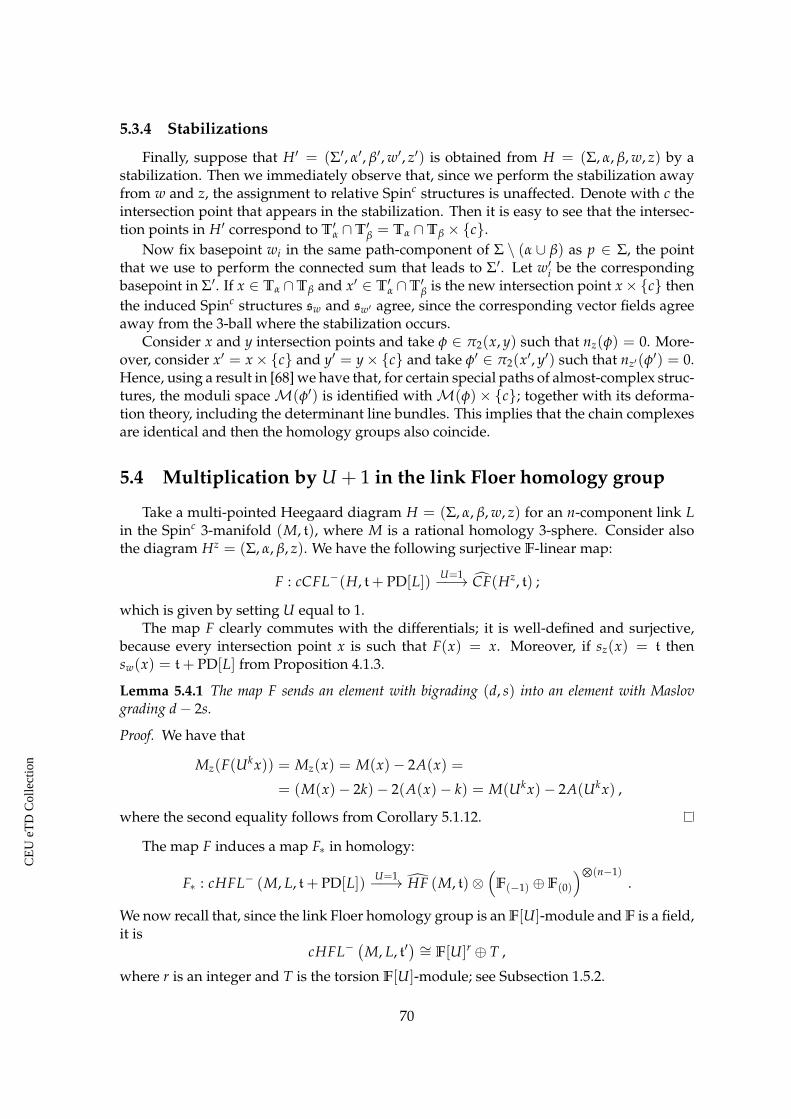
5.3.4 Stabilizations
Finally, suppose that H′ = (Σ′, α′, β′, w′, z′) is obtained from H = (Σ, α, β, w, z) by astabilization. Then we immediately observe that, since we perform the stabilization awayfrom w and z, the assignment to relative Spinc structures is unaffected. Denote with c theintersection point that appears in the stabilization. Then it is easy to see that the intersec-tion points in H′ correspond to T′α ∩T′β = Tα ∩Tβ × {c}.
Now fix basepoint wi in the same path-component of Σ \ (α ∪ β) as p ∈ Σ, the pointthat we use to perform the connected sum that leads to Σ′. Let w′i be the correspondingbasepoint in Σ′. If x ∈ Tα ∩Tβ and x′ ∈ T′α ∩T′β is the new intersection point x× {c} thenthe induced Spinc structures sw and sw′ agree, since the corresponding vector fields agreeaway from the 3-ball where the stabilization occurs.
Consider x and y intersection points and take φ ∈ π2(x, y) such that nz(φ) = 0. More-over, consider x′ = x× {c} and y′ = y× {c} and take φ′ ∈ π2(x′, y′) such that nz′(φ
′) = 0.Hence, using a result in [68] we have that, for certain special paths of almost-complex struc-tures, the moduli spaceM(φ′) is identified withM(φ)× {c}; together with its deforma-tion theory, including the determinant line bundles. This implies that the chain complexesare identical and then the homology groups also coincide.
5.4 Multiplication by U + 1 in the link Floer homology group
Take a multi-pointed Heegaard diagram H = (Σ, α, β, w, z) for an n-component link Lin the Spinc 3-manifold (M, t), where M is a rational homology 3-sphere. Consider alsothe diagram Hz = (Σ, α, β, z). We have the following surjective F-linear map:
F : cCFL−(H, t+ PD[L]) U=1−−→ CF(Hz, t) ;
which is given by setting U equal to 1.The map F clearly commutes with the differentials; it is well-defined and surjective,
because every intersection point x is such that F(x) = x. Moreover, if sz(x) = t thensw(x) = t+ PD[L] from Proposition 4.1.3.
Lemma 5.4.1 The map F sends an element with bigrading (d, s) into an element with Maslovgrading d− 2s.
Proof. We have that
Mz(F(Ukx)) = Mz(x) = M(x)− 2A(x) =
= (M(x)− 2k)− 2(A(x)− k) = M(Ukx)− 2A(Ukx) ,
where the second equality follows from Corollary 5.1.12.
The map F induces a map F∗ in homology:
F∗ : cHFL− (M, L, t+ PD[L]) U=1−−→ HF (M, t)⊗(
F(−1) ⊕F(0)
)⊗(n−1).
We now recall that, since the link Floer homology group is an F[U]-module and F is a field,it is
cHFL−(
M, L, t′) ∼= F[U]r ⊕ T ,
where r is an integer and T is the torsion F[U]-module; see Subsection 1.5.2.
70
CE
UeT
DC
olle
ctio
n

Lemma 5.4.2 The following two statements hold:
1. we have that F(x) = 0 and x is homogeneous with respect to the Alexander grading if andonly if x = 0;
2. we have that F∗[x] = [0] and [xi] is homogeneous with respect to the Alexander grading, forevery i = 1, ..., r, if and only if [x] is torsion. Here the [xi]’s are a decomposition of [x] in thetorsion-free quotient of cHFL− (M, L, t+ PD[L]).
Proof. 1. The if implication is trivial. For the only if, suppose that F(x) = 0; this givesthat
x = (1 + U)λ1(U)y1 + ... + (1 + U)λt(U)yt ,
where λi(U) ∈ F[U] for every i = 1, ..., t and y1, ..., yt are all the intersection pointsthat induce the Spinc structure t.
Since each yi is homogeneous and the monomial U drops the Alexander grading byone, we have that λi(U) = 0 for every i = 1, ..., t and then x = 0.
2. Again the if implication is trivial. Now we have that
[x] =r
∑i=1
[xi] + [x]T ,
where [x]T is the projection of [x] on the torsion submodule T. Since F∗[x] = [0], it is
[x] = (1 + U)[z] = (1 + U)λ′1(U)[z1] + ... + (1 + U)λ′r(U)[zr] + [x]T ;
where [xi] = (1 + U)λ′i(U)[zi] for every i = 1, ..., r and the [zi]′s are a homogeneous
basis of the torsion-free quotient.
The same argument of 1 implies that the polynomials λ′i(U) are all zero and then[x] = [x]T.
Now we use Lemma 5.4.2 to show that there is a correspondence between the torsion-free quotient of the link Floer homology group and the multi-pointed hat Heegaard Floerhomology.
Theorem 5.4.3 If L is an n-component link in a rational homology 3-sphere M then there existsan isomorphism of F[U]-modules
cHFL− (M, L, t+ PD[L])T
−→(HF (M, t)⊗F F[U]
)⊗F[U]
(F[U](−1) ⊕F[U](0)
)⊗(n−1);
which sends a homology class of bigrading (d, s) into one of Maslov grading d− 2s.
Proof. We just have to show that F∗ sends {[z1], ..., [zr]}, a homogeneous F[U]-basis ofthe torsion-free quotient of cHFL− (M, L, t+ PD[L]), into an F-basis of X = HF (M, t)⊗(
F(−1) ⊕F(0)
)⊗(n−1). Statement 1 in Lemma 5.4.2 tells us that F∗ is surjective. In fact, if
[y] ∈ X then it is 0 = ∂zy = F(∂−x); where F(x) = y. We apply Lemma 5.4.2 to ∂−(x),
71
CE
UeT
DC
olle
ctio
n

since we can suppose that both x and y are homogeneous, and we obtain that ∂−(x) = 0;then [x] is a homology class. At this point, it is easy to see that the set {F∗[z1], ..., F∗[zr]} isa system of generators of X .
In order to prove that F∗[z1], ..., F∗[zr] are also linearly independent in X we supposethat there is a subset
{F∗[zi1 ], ..., F∗[zik ]
}such that
F∗[zi1 ] + ... + F∗[zik ] = F∗[zi1 + ... + zik ] = [0] .
Then we apply Statement 2 of Lemma 5.4.2 to [zi1 + ... + zik ] and we obtain that it is atorsion class. This is a contradiction, because [zi1 ], ..., [zik ] are part of an F[U]-basis of atorsion-free F[U]-module.
72
CE
UeT
DC
olle
ctio
n

Chapter 6
Legendrian and contact invariantsfrom open book decompositions
6.1 Legendrian Heegaard diagrams
6.1.1 Heegaard diagrams through abstract open books
In this chapter we introduce a specific type of Heegaard diagrams, obtained fromadapted open book decompositions, that we call Legendrian Heegaard diagrams. Givenan adapted open book decomposition (B, π, A), compatible with the triple (L, M, ξ), seeSubsection 4.2.1, a Legendrian Heegaard diagram is a multi-pointed Heegaard diagramD = (Σ, α, β, w, z) which is obtained from the abstract open book associated to (B, π, A),defined in Subsection 4.2.2.
Denote such abstract open book with (S1, Φ,A, z, w). We have that S±1 = π−1(±1).The sets of arcs in S1 are A = {a1, ..., a2g+l+n−2} and B = {b1, ..., b2g+l+n−2}, as in Figure
S ∪−S
β1 α1
β2α2
α3β3z1
w1
z2
w2
Figure 6.1: A diagram for the standard Legendrian 2-unlink in (S3, ξst), obtained from anopen book decomposition with page as in Figure 4.5.
4.8. We recall that g is the genus of S1, while l is the number of its boundary componentsand n is the number of components of L. We define ai and bi for i = 1, ..., 2g + l + n− 2 asin Subsection 4.2.2.
Then D is gotten as follows:
• the surface Σ is S1 ∪ −S−1; since π is a locally trivial fibration the pages S1 and S−1are diffeomorphic, but we reverse the orientation of the second one when we gluethem together;
73
CE
UeT
DC
olle
ctio
n

• the curves are given by αi = bi ∪ bi and βi = ai ∪ ai for every i = 1, ..., 2g + l + n− 2;
• the z’s and the w’s are the set of baspoints that we introduced in Section 4.2.
In the settings of Chapter 4 the Legendrian Heegaard diagram (Σ, α, β, w, z) is a diagramfor the (smooth) link L in the 3-manifold −M, see [72] and Subsection 4.2.2 before, that isM considered with the opposite orientation. We remark that here α and β are swappedwith respect to the convention of Ozsváth and Szabó, which is the one we used in Chapter4. See Figure 6.1 for an example.
We observe that, given (B, π, A), the only freedom in the choice of the Legendrian Hee-gaard diagram is in the arcs b1, ..., b2g+l+n−2 inside S−1, which can be taken in the isotopyclass of Φ(b1), ...Φ(b2g+l+n−2).
Proposition 6.1.1 Suppose D = (Σ, α, β, w, z) is a Legendrian Heegaard diagram given by anadapted open book decomposition compatible with (L, M, ξ), where M is a rational homology 3-sphere. Then D is always admissible up to isotopy of the arcs in B.
Proof. It follows from Lemma 5.1.5 and [77].
Our strategy is to study how Legendrian isotopic triples are related to one another,which means to define a finite set of moves between two adapted open book decomposi-tions. Then find chain maps Ψ(D1,D2) for each move, that induce isomorphisms in homol-ogy, which will be particular cases of the maps in Section 5.3.
6.1.2 Global isotopies
We want to show that, given two Legendrian isotopic links L1, L2 ↪→ (M, ξ), two openbook decompositions (Bi, πi, Ai), compatible with the triples (Li, M, ξ), are related by afinite sequence of moves. The first lemma follows easily.
Lemma 6.1.2 Let us consider an adapted open book decomposition (B1, π1, A1), compatible withthe triple (L1, M, ξ), and suppose that there is a contact isotopy of (M, ξ), sending L1 into L2.
Then the time-1 map of the isotopy is a diffeomorphism F : M → M such that(
F(B1), π1 ◦F−1, F(A1)
)is an adapted open book decomposition, compatible with (L2, M, ξ).
Proof. The proof of the statement can be checked without effort.
This lemma says that, up to global contact isotopies, we can consider (Bi, πi, Ai) to beboth compatible with a triple (L, M, ξ), where the link L is Legendrian isotopic to Li for i =1, 2. In other words, we can just study the relation between two open book decompositionscompatible with a single triple (L, M, ξ).
6.1.3 Positive stabilizations
Let us start with a pair (S, Φ). A positive stabilization of (S, Φ) is the pair(
S, Φ)
obtained in the following way:
• the surface S is given by adding a 1-handle H to S;
• the monodromy Φ is isotopic to Φ′ ◦ Dγ. The map Φ′ concides with Φ on S and it isthe Identity on H. While Dγ is the right-handed Dehn twist along a curve γ; whichintersects S ∩ H transversely precisely in the attaching sphere of H. See Figure 6.2.
74
CE
UeT
DC
olle
ctio
n
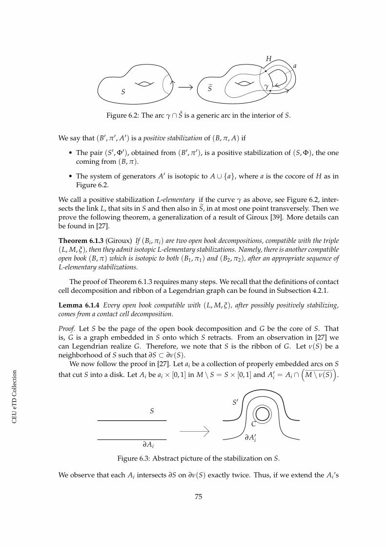
S S γ
Ha
Figure 6.2: The arc γ ∩ S is a generic arc in the interior of S.
We say that (B′, π′, A′) is a positive stabilization of (B, π, A) if
• The pair (S′, Φ′), obtained from (B′, π′), is a positive stabilization of (S, Φ), the onecoming from (B, π).
• The system of generators A′ is isotopic to A ∪ {a}, where a is the cocore of H as inFigure 6.2.
We call a positive stabilization L-elementary if the curve γ as above, see Figure 6.2, inter-sects the link L, that sits in S and then also in S, in at most one point transversely. Then weprove the following theorem, a generalization of a result of Giroux [39]. More details canbe found in [27].
Theorem 6.1.3 (Giroux) If (Bi, πi) are two open book decompositions, compatible with the triple(L, M, ξ), then they admit isotopic L-elementary stabilizations. Namely, there is another compatibleopen book (B, π) which is isotopic to both (B1, π1) and (B2, π2), after an appropriate sequence ofL-elementary stabilizations.
The proof of Theorem 6.1.3 requires many steps. We recall that the definitions of contactcell decomposition and ribbon of a Legendrian graph can be found in Subsection 4.2.1.
Lemma 6.1.4 Every open book compatible with (L, M, ξ), after possibly positively stabilizing,comes from a contact cell decomposition.
Proof. Let S be the page of the open book decomposition and G be the core of S. Thatis, G is a graph embedded in S onto which S retracts. From an observation in [27] wecan Legendrian realize G. Therefore, we note that S is the ribbon of G. Let ν(S) be aneighborhood of S such that ∂S ⊂ ∂ν(S).
We now follow the proof in [27]. Let ai be a collection of properly embedded arcs on Sthat cut S into a disk. Let Ai be ai × [0, 1] in M \ S = S× [0, 1] and A′i = Ai ∩
(M \ ν(S)
).
S
∂Ai
∂A′i
C
S′
Figure 6.3: Abstract picture of the stabilization on S.
We observe that each Ai intersects ∂S on ∂ν(S) exactly twice. Thus, if we extend the Ai’s
75
CE
UeT
DC
olle
ctio
n

into ν(S) so that their boundaries lie on G then the twisting of S, and hence ξ, along ∂Aiwith respect to Ai is -1,0 or 1. If the value of all the twisting is -1 then we have a contactcell decomposition, because the contact structure restricted to the complement of S is tight.Then we just need to see how to reduce the twisting of ξ along ∂Ai.
Suppose ∂Ai has twisting 0. Then positively stabilize S as shown in Figure 6.3. Notethat the curve C can be assumed to be Legendrian and bounds a disk E in M. Now isotopeG across E to get a new Legendrian graph with all the Aj’s unchanged except that Ai isreplace with the disk A′i obtained from Ai by isotoping across E. We also add C to G andadd E to the 2-skeleton.
Clearly the twisting of ξ along E is -1. Thus we can reduce the twisting of ξ along ∂Aias needed and after sufficiently many positive stabilizations we have an open book thatcomes from a contact cell decomposition.
We observe that, in the proof of Lemma 6.1.4, we only use L-elementary stabilizations.We apply Lemma 6.1.4 to both (Bi, πi). Obviously, we can also suppose that the 1-skeletonof (M, ξ) that we have in the beginning is a subgraph of the one after the stabilizations. Atthis point, we need to know how to relate two different contact cell decompositions for thesame triple (L, M, ξ). To do this we use the following proposition.
Proposition 6.1.5 Given two contact cell decompositions, for the same contact manifold, we havethat they are related by a finite sequence of the following moves:
1. a subdivision of a 2-cell by a Legendrian arc, intersecting the dividing set in one point;
2. add a 1-cell c′ and a 2-cell E so that ∂E = c′ ∪ c; where c is part of the original 1-skeletonand tb(∂E) = −1;
3. add a 2-cell E whose boundary is already in the 1-skeleton and tb(∂E) = −1.
Proof. The proof follows from standard results in contact topology.
The definition of dividing set of a convex surface is in Subsection 3.1.1. Clearly, we
E
L
ΓE
c
c′
c′1 c′2
Figure 6.4: The arc ΓE is the dividing set of the 2-cell E.
have that Move 1 corresponds to an L-elementary stabilization of (B1, π1), while Move 3does not change the open book at all. For Move 2 on the other hand we have to reasonmore. In fact it can happen that the arc c in the original 1-skeleton intersects the link Ltransversely in more than one point. We solve this problem by applying other appropriateMoves 1 as in Figure 6.4. We observe that we obtain the same contact cell decompositionif we apply a sequence of Moves 2, using the arcs c′i, which now will give L-elementarystabilizations. To complete the proof we only need the following lemma.
76
CE
UeT
DC
olle
ctio
n

Lemma 6.1.6 Suppose (Bi, πi) are two open books, compatible with (L, M, ξ), which come fromthe same contact cell decomposition. Then we have that (B1, π1) is isotopic to (B2, π2).
Proof. First we have that the pages π−11 (1) and π−1
2 (1) are isotopic, because it is easy tosee that the ribbon of the 1-skeleton is unique up to isotopy. Then we can suppose thatthe bindings coincide and S = π−1
i (1) for i = 1, 2. Now, we have that M \ S fibers alongthe interval (0, 1) in two different ways. At this point, since (0, 1) is contractible the twofibrations result to be trivial and then isotopic. It remains to see what happens when weglue S back.
The two open books induce monodromies Φ1 and Φ2 on S and they are conjugatebecause otherwise, from Corollary 4.2.3, the resulting open books would be compatiblewith non contactomorphic contact manifolds; but this is impossible. Then the fact thatthe monodromies are in the same conjugacy class tells us precisely that we can extend theisotopy on S and this completes the proof.
In other words, we may need to stabilize both open book decompositions many timesand eventually we obtain other two open book decompositions
(B, π, Ai
), both compati-
ble with L ↪→ (M, ξ); which is contact isotopic to (Li, M, ξi) for i = 1, 2.
6.1.4 Admissible arc slides
In this subsection we use the terminology introduced in Subsection 4.2.1. Take anadapted system of generators A for an n-component link L, lying inside a surface S.We define admissible arc slide, a move that change A = {a1, ..., ai, ..., aj, a2g+l+k−2} into
L
Lai
ai + aj
aj aj
S S
Figure 6.5: The arc ai + aj is obtained by sliding aj over ai.
A′ = {..., ai + aj, ..., aj, ...}; where aj is not a distinguished arc and one of the endpoints ofai and aj are adjacent, like in Figure 6.5. We can prove the following proposition.
Proposition 6.1.7 Let us consider two open book decompositions (B, π, Ai), compatible with theLegendrian link L ↪→ (M, ξ). Then, after a finite number of admissible arc slides and isotopies onAi, the open books coincide.
We need two preliminary lemmas.
Lemma 6.1.8 An admissible arc slide, from A to A′, can be inverted. In the sense that we canperform another admissible arc slide, now from A′ to A′′, such that A′′ is isotopic to A.
Proof. If the arc slide changes the arc ai into ai + aj then it is easy to see that we can justslide ai + aj over an arc a′j, isotopic to aj; in a way that ai + aj + a′j is isotopic to ai.
Lemma 6.1.9 Suppose that we perform an admissible arc slide that changes ai into ai + aj. Thenwe have the following facts:
77
CE
UeT
DC
olle
ctio
n

a) The set {a1, ..., a2g+l−1} is a basis of H1(S, ∂S; F) and i 6 2g + l− 1 if and only if {a1, ..., ai +aj, ..., a2g+l−1} is a basis of H1(S, ∂S; F),
b) The arc ai is distinguished if and only if ai + aj is a distinguished arc,
c) The arc ai is separating if and only if ai + aj is a separating arc,
d) The arc ai is dead if and only if ai + aj is a dead arc.
Proof. a) Obviously, the arc ai + aj represents the sum of the relative homology classes ofai and aj. At this point we just need basic linear algebra.
b) This claim is trivial.
c) We take {a1, ..., a2g+l−1} as a basis of the first relative homology group of S. We cansuppose that i > 2g + l. This is because if ai is the only separating arc for a componentof S \ {a1, ..., a2g+l−1} then ai is homologically trivial; otherwise, we can switch ai withanother separating arc for the same component.
Now, if ai + aj is not a separating arc then S \ {a1, ..., a2g+l−1, ai + aj} should remainconnected, but this is impossible because {a1, ..., a2g+l−1} is a basis.
The other implication follows easily from Lemma 6.1.8.
d) It follows from b) and c).
The strategy of the proof of Proposition 6.1.7 is, say S1, ..., Sn and S′1, ..., S′n are the com-ponents of S minus the separating arcs of A1 and A2 respectively, we modify all the sep-arating arcs, in both A1 and A2, with admissible arc slides; in order for Si to concide withS′i for every i = 1, ..., n. Moreover, we also want that each separating arc in A1 becomesisotopic to a separating arc in A2.
At the end, the components of S minus the separating arcs will be n surfaces, each onecontaining a component of L, a distinguished arc and the same number of dead arcs. We
S1a2g+l
a1a1
Dead arcs
L1S1
L1a1
a1
a2g+l
ai
Figure 6.6: Case 1 is on the left. The figure shows a portion of S \ A1.
conclude applying n times a result in [57], which proves the claim in the case of Legendrianknots.
Proof of Proposition 6.1.7. We want to prove that there is an adapted system of generators Afor L in S1 = π−1(1) such that A is obtained, from A1 and A2, by a sequence of admissiblearc slides (and isotopies).
We start from the component S1. We can suppose that ∂S1 contains the separating arca2g+l ⊂ A3
1, the set of separating arcs in ⊂ A1, and the distinguished arc a1 ⊂ A11, the set
of distinguished arcs in A1, with almost adjacent endpoints. We can have two cases: in
78
CE
UeT
DC
olle
ctio
n

the first one there are no other separating arcs in the portion of ∂S1 on the opposite sideof a2g+l . In the second case they appear; possibly more than one, but we can suppose thatthere is exactly one of them. See Figure 6.6.
Case 1. When we consider S′1, which contains the same component of L that is in S1, aftersome arc slides we have that it appears as in Figure 6.6 (left). This is because in the
S1
a2g+l
a1 a1Dead arcs
L1
a′1
a′2g+l
Figure 6.7: There are no other separating arcs, except for a2g+l in S1.
same figure we see that S1 is split in two pieces by L1 and the innermost one is notconnected in any way to other components of S; in fact there are no separating arcson that side. This means that the same holds for S′1 too. At this point it is easy tosee that S1 can be modified to be like in Figure 6.7; more explicitly, the separatingarcs are parallel and the distinguished arcs lie in the region where L1 is.
Case 2. As before we have that also S′1 appears like in the right part of Figure 6.6 (alwaysafter some arc slides). The reason is the same of previous case. Hence, now we canmodify S1 to be like in Figure 6.8; just in the same way as we did in Case 1.
We have obtained that the separating arcs are fixed on S1 and S′1 and then the surfacesnow have isotopic boundaries. Hence, we can move to another component S2, whose
S1
L1
a1a1
a2g+l
ai
a′i
a′2g+l
a′1
Figure 6.8: There are exactly two separating arcs, namely a2g+l and ai in S1.
79
CE
UeT
DC
olle
ctio
n

boundary contains a separating arc that has not yet been fixed, and we repeat the sameprocess described before. We may need to slide some separating arcs over the ones that wealready fixed in the previous step, but this is not a problem. We just iterate this procedureuntil all the Si coincides with S′i and this completes the proof.
The results in this section prove the following theorem.
Theorem 6.1.10 If L1, L2 ↪→ (M, ξ) are Legendrian isotopic links then the open book decom-positions (Bi, πi, Ai), which are compatible with the corresponding triples, are related by a finitesequence of global contact isotopies, positive stabilizations and admissible arc slides.
Proof. It follows immediately from Propositions 6.1.1 and 6.1.7, Lemma 6.1.2 and Theorem6.1.3.
Though they are easy to deal with, we must not forget that, when we define the cor-responding Legendrian Heegaard diagrams, we need to consider the choices of the mon-odromy and the families of arcs and basepoints inside their isotopy classes.
6.2 The Legendrian and transverse invariants
In this subsection we identify a cycle in the link Floer chain complexes that we pre-viously introduced. The corresponding homology class will be our Legendrian invariant.Let us consider the only intersection point of D = (Σ, α, β, w, z) which lies in the page S1.We recall that, in general, the intersection points live in the space Tα ∩Tβ, but they can berepresented inside Σ. We denote this element with L(D).
Proposition 6.2.1 The intersection point L(D) is such that ∂−L(D) = 0 and then L(D) is acycle in cCFL−
(D, tL(D)
); where tL(D) is the Spinc structure that it induces on −M.
Proof. Every φ ∈ π2(L(D), y) such that µ(φ) = 1, where y ∈ Tα ∩ Tβ, has the propertythat nz(φ) > 0. The claim follows easily from the definition of the differential.
At the end of the chapter we show that more can be said on the Spinc structure tL(D).Now we want to show that the isomorphism class of the element [L(D)] inside the homol-ogy group cHFL−
(−M, L, tL(D)
)is a Legendrian invariant of the triple (L, M, ξ).
Let us be more specific: we consider a Legendrian link L ↪→ (M, ξ) in a rational ho-mology contact 3-sphere; we associate two open book decompositions compatible with(L, M, ξ), say (B1, π1, A1) and (B2, π2, A2), and these determine (up to isotopy) two Legen-drian Heegaard diagrams, that we call D1 = (Σ1, α1, β1, w1, z1) and D2 = (Σ2, α2, β2, w2, z2)respectively. Then we want to find a chain map
Ψ(D1,D2) : cCFL−(D1, t) −→ cCFL−(D2, t) , (6.1)
that induces an isomorphism in homology, preserves the bigrading and it is such that
Ψ(D1,D2)(L(D1)) = L(D2) ,
where t = tL(D1) = tL(D2) ∈ Spinc (−M). This is done in order to prove the followingtheorem.
80
CE
UeT
DC
olle
ctio
n

Theorem 6.2.2 Let us consider a Legendrian Heegaard diagram D, given by an open book com-patible with a triple (L, M, ξ), where M is a rational homology 3-sphere and L is an n-componentLegendrian link.
Let us take the cycle L(D) ∈ cCFL−(D, tL(D)). Then, the isomorphism class of [L(D)] incHFL−
(−M, L, tξ
)is a Legendrian invariant of (L, M, ξ) and we denote it with L(L, M, ξ).
Furthermore, the Spinc structure tL(D) coincides with tξ + PD[L].
Here we denote with tξ the Spinc structure induced on M by ξ.
Proposition 6.2.3 Given a contact 3-manifold (Y, ζ) we have that ζ induces a Spinc structure tζon Y.
Proof. The contact structure ζ gives a cooriented 2-plane field π on Y. Hence, if we takethe isotopy class of the vector field orthogonal to π and oriented coherently with Y then,according to Turaev definition, we obtain a Spinc structure on Y that we denote with tζ .
In Section 5.1 we define another chain complex(
CFL(D, t), ∂)
for every Spinc structuret on −M, whose homology is
HFL(−M, L, t) .
The intersection point L(D) is a cycle also in CFL(D, t) and it also determines the Spinc
structure tL(D). Then the same procedure will show that the homology class [L(D)] in
HFL(−M, L, t) is also a Legendrian invariant of L.
Theorem 6.2.4 The isomorphism class of [L(D)] in HFL(−M, L, tξ + PD[L]
)is a Legendrian
invariant of (L, M, ξ) and we denote it with L(L, M, ξ). Moreover, if L(L, M, ξ) is non-zero thenL(L, M, ξ) is also non-zero.
We recall that in Section 3.3 we give the definition of the transverse push-off TL of aLegendrian link L. In the same way, if T is a transverse link then we can define a Legen-drian approximation LT of T. The procedure is described in [26]. The Legendrian link LTis not well-defined up to Legendrian isotopy, but only up to negative stabilizations, seeSection 3.5. Then we can also define transverse invariants from these link Floer homologygroups by taking
T(T, M, ξ) = L(LT, M, ξ) and T(T, M, ξ) = L(LT, M, ξ) ,
where LT is a Legendrian approximation of T.
Theorem 6.2.5 The isomorphism classes T(T, M, ξ) in cHFL−(−M, T, tξ + PD[T]
), and
T(T, M, ξ) in HFL(−M, T, tξ + PD[T]
), are transverse link invariants. Furthermore, we have
that T(T, M, ξ) has the same non-vanishing property of L.
In the case of knots the invariants L and T have been introduced first in [57].
6.3 Proof of the invariance
6.3.1 Global isotopies and admissible arc slides
If two open book decompositions are related by a global isotopy then it easy to see thatthe induced abstract open book coincide, up to conjugation of the monodromy and isotopyof the curves and the basepoints in the diagrams.
81
CE
UeT
DC
olle
ctio
n

Hence, let us consider an abstract open book (S, Φ,A, z, w) and recall that in S we havetwo set of arcs A and B, as explained in Subsection 4.2.2. The first check is easy: in fact if weperturb the basepoints inside the corresponding components of S \ (A ∪ B) then even thecomplex (cCFL−(D, t), ∂−) does not change; where D is a Legendrian Heegaard diagramobtained from (S, Φ,A, z, w). The same is true for an isotopy of S.
Now for what it concerns S we do not have problems, but when we define the chaincomplex we also consider the closed surface Σ, obtained by gluing together S and −S. Westill have some choices on −S, in fact by Proposition 6.1.1 we may need to modify the arcsB in their isotopy classes to achieve admissibility for D = (Σ, α, β, w, z). Then the proofrests on the following proposition.
Proposition 6.3.1 Suppose that two curves in a Heegaard diagram are related by the move shownin Figure 5.3. Then we can find a map Ψ(D1,D2) as in Equation (6.1).
Proof. The map Ψ(D1,D2) is constructed using a Hamiltonian diffeomorphism of the surface,as described in Subsection 5.3.2. Since the new disks appear in −S, we have that L(D1) issent to L(D2) which both lie in S.
An arc slide {..., ai, ..., aj, ...} → {..., ai + aj, ..., aj, ...} in S corresponds to a handleslide{..., αi, ..., αj, ...} → {..., α′i, ..., αj, ...} in Σ, where α′i = ai + aj ∪ ai + aj ⊂ Σ. Thus, a chainmap Ψ(D1,D2), which induces an isomorphism in homology, is obtained by counting holo-morphic triangles, as explained in Subsection 5.3.3. The admissibility of the arc slide isrequired only to avoid crossing a basepoint in w.
Remember that for every arc slide we actually have two handleslides. In fact we needto slide both the α and the β curves.
The fact that Ψ(D1,D2)(L(D1)) = L(D2) follows from [47]; where the arc slides invari-ance is proved in the open books setting.
6.3.2 Invariance under positive stabilizations
At this point, in order to complete the proof of the invariance of [L(D)], it would beenough to define Ψ(D,D+), such that Ψ(D,D+)(L(D)) = L(D+), in the case where D and D+
are obtained from an open book and one of its positive stabilizations.Since we have already proved invariance under admissible arc slides, we can complete
the open books (B, π) and (B+, π+) with every possible adapted system of generators andthen eventually define the map Ψ(D,D+).
Proposition 6.3.2 Let us call S = Sg,l = π−1(1) ⊃ L the page over 1 of (B, π). Then we canalways find A, an adapted system of generators for L in S, with the property that A is disjoint fromthe arc γ′ = γ ∩ S; where γ is the curve that we used to perform the L-elementary stabilization.
Proof. We have to study four cases:
a) The arc γ′ intersects L (transversely in one point),
b) The intersection γ′ ∩ L is empty and γ′ does not disconnect S,
c) The intersection γ′ ∩ L is empty, the arc γ′ disconnects S and L is not contained in oneof the two resulting connected components of S,
d) The intersection γ′ ∩ L is empty, the arc γ′ disconnects S and the link L lies in one of theresulting connected components of S.
82
CE
UeT
DC
olle
ctio
n

Let us start with Case a). We observe that γ′ does not disconnect S; in fact if this was thecase then a component of L would be split inside the two resulting components of S, thuswe would have at least another intersection point between L and γ′; which is forbidden.We define A = {a1, ..., a2g+l+n−2} as follows. Take a1 as a push-off of γ′; clearly a1 is adistinguished arc, because it intersects L1, a component of L, in one point. Now call a′ thearc given by taking a push-off of L1 and extend it through a1, on one side of L1; this isthe same procedure described in the proof of Theorem 4.2.1. If a′ disconnects S into S1, S2and there are components of L that lie in both Si then we take a′ as a separating arc; thuswe extend {a1, a′} to an adapted system of generators A by using Theorem 4.2.1. On theother hand if L is contained in S2 and S1 is empty then we consider {a1, a′′}; where a′′
is another push-off of L1, this time extended through a1 on the other side of L1. We stillhave problems when a′ does not disconnect S. We can fix this by taking {a1, a′, a′′}; whichtogether disconnect S into two connected components, one of them containing only L1 andthe other one L \ L1. Again we extend the set {a1, a′, a′′} to A applying Theorem 4.2.1.
The other three cases are easier. In Case b) we just denote with an+1 the push-off of γ′
and we complete it to A.In Case c) we denote with a2g+l our push-off of γ′ and we take it as a separating arc.
Then we can complete it to A.Finally, Case d) is as follows. Since in this case the push-off is trivial in homology, and
it bounds a surface disjoint from L, we can actually ignore it and easily find a set A whichnever intersects γ′.
Now we have the abstract open book (S, Φ,A, z, w), obtained from (B, π, A). Denote
with (S+, Φ+,A+, z, w) the one coming from (B+, π+, A+), where S+ = (π+)−1 (1) is Swith a 1-handle attached; Φ+ = Φ′ ◦ Dγ where Φ′ coincides with Φ on S, extended withthe Identity on the new 1-handle; and A+ = A ∪ {a} with a being the cocore of the new1-handle (see Figure 6.2). Then we call D and D+ the corresponding Legendrian Heegaarddiagrams.
We define Ψ(D,D+) in the following way. For every x ∈ Tα ∩Tβ|tL(D)it is
Ψ(D,D+)(x) = x′ ;
where x′ = x ∪ {a ∩ b} with b being the arc in strip position with a, as in Figure 4.8.It results that Ψ(D,D+) is a chain map because the curve α = b ∪ b only intersects the
curve β = a∪ a, and moreover it is α∩ β = {1 pt}, since we choose A+ in a way that everyarc in it is disjoint from γ′. We have that Ψ(D,D+) induces an isomorphism in homology,because it is an isomorphism also on the level of chain complexes, and sends L(D) intoL(D+).
6.3.3 Invariance theorems
We prove our main results in this chapter, which shows the invariance of L and T. Theclaim about the Spinc structure tL(D) is studied in Section 6.4.
Proof of Theorem 6.2.2. We proved that L(D) is a cycle in Proposition 6.2.1. The invariancefollows from the results obtained in this section: in fact, we proved that if D1 and D2 areLegendrian Heegaard diagrams, representing Legendrian isotopic links, then we have achain map Ψ(D1,D2) that preserves the bigrading and the Spinc structure and sends L(D1)to L(D2).
83
CE
UeT
DC
olle
ctio
n

We note that the invariant can be a U-torsion class in the group cHFL−(−M, L, tL(D)
),
which means that there is a k > 0 such that Uk · L(L, M, ξ) = [0]. Moreover, the cycleL(D) possesses a bigrading (d, s); such bigrading is induced on the invariant L(L, M, ξ),because all the maps Ψ defined in this section preserves both the Maslov and the Alexandergrading.
Proof of Theorem 6.2.4. The proof of this theorem is the same as the one of Theorems6.2.2 and 6.2.5, except for the non-vanishing property, which follows from the fact thatCFL(D, tL(D)) is a quotient of cCFL−(D, tL(D)).
6.4 A remark on the Ozsváth-Szabó contact invariant
Now we spend a few words about the Ozsváth-Szabó contact invariant c(ξ), intro-duced in [70].
Given a Legendrian Heegaard diagram D. Let us call c(D) the only intersection pointwhich lies on the page S1 as before, but now considered as an element in
(CF(D, tc(D)), ∂z
).
The proof of Proposition 6.2.1 says that c(D) is also a cycle. Moreover, we have the follow-ing theorem.
Theorem 6.4.1 (Ozsváth and Szabó) Let us consider a Legendrian Heegaard diagram D witha single basepoint z, given by an open book compatible with a pair (M, ξ), where M is a rationalhomology 3-sphere. Let us take the cycle c(D) ∈ CF(D, tc(D)).
Then the isomorphism class of [c(D)] ∈ HF(−M, tc(D)
)is a contact invariant of (M, ξ) and
we denote it with c(M, ξ). Furthermore, we have the following properties:
• the Spinc structure tc(D) coincides with tξ ;
• the Maslov grading of c(D) is given by Mz(c(D)) = −d3(M, ξ).
The proof of this theorem comes from [70], where Ozsváth and Szabó first define theinvariant c(M, ξ), and [47], where Honda, Kazez and Matic give the reformulation usingopen book decompositions that we use in this thesis.
Furthermore, now we can see which is the Spinc structure induced by L(D).
Corollary 6.4.2 The intersection point L(D) induces the Spinc structure tξ + PD[L].
This completes the proof of Theorem 6.2.2.
Proof of Corollary 6.4.2. We recall that
sw(L(D))− sz(L(D)) = PD[L]
from Proposition 4.1.3. Then we have that
tL(D) = sw(L(D)) = sz(L(D)) + PD[L] = tc(D) + PD[L] = tξ + PD[L] ,
from Theorem 6.4.1.
84
CE
UeT
DC
olle
ctio
n
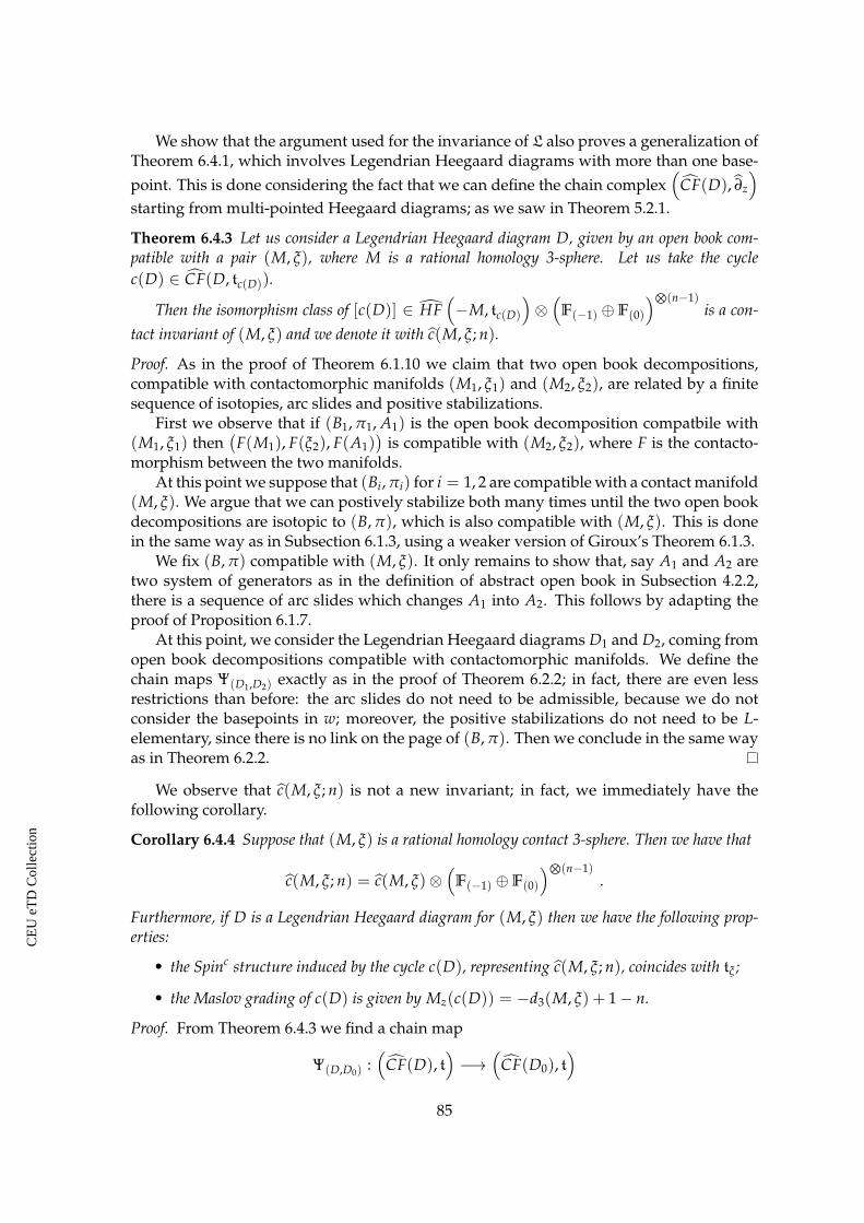
We show that the argument used for the invariance of L also proves a generalization ofTheorem 6.4.1, which involves Legendrian Heegaard diagrams with more than one base-point. This is done considering the fact that we can define the chain complex
(CF(D), ∂z
)starting from multi-pointed Heegaard diagrams; as we saw in Theorem 5.2.1.
Theorem 6.4.3 Let us consider a Legendrian Heegaard diagram D, given by an open book com-patible with a pair (M, ξ), where M is a rational homology 3-sphere. Let us take the cyclec(D) ∈ CF(D, tc(D)).
Then the isomorphism class of [c(D)] ∈ HF(−M, tc(D)
)⊗(
F(−1) ⊕F(0)
)⊗(n−1)is a con-
tact invariant of (M, ξ) and we denote it with c(M, ξ; n).
Proof. As in the proof of Theorem 6.1.10 we claim that two open book decompositions,compatible with contactomorphic manifolds (M1, ξ1) and (M2, ξ2), are related by a finitesequence of isotopies, arc slides and positive stabilizations.
First we observe that if (B1, π1, A1) is the open book decomposition compatbile with(M1, ξ1) then
(F(M1), F(ξ2), F(A1)
)is compatible with (M2, ξ2), where F is the contacto-
morphism between the two manifolds.At this point we suppose that (Bi, πi) for i = 1, 2 are compatible with a contact manifold
(M, ξ). We argue that we can postively stabilize both many times until the two open bookdecompositions are isotopic to (B, π), which is also compatible with (M, ξ). This is donein the same way as in Subsection 6.1.3, using a weaker version of Giroux’s Theorem 6.1.3.
We fix (B, π) compatible with (M, ξ). It only remains to show that, say A1 and A2 aretwo system of generators as in the definition of abstract open book in Subsection 4.2.2,there is a sequence of arc slides which changes A1 into A2. This follows by adapting theproof of Proposition 6.1.7.
At this point, we consider the Legendrian Heegaard diagrams D1 and D2, coming fromopen book decompositions compatible with contactomorphic manifolds. We define thechain maps Ψ(D1,D2) exactly as in the proof of Theorem 6.2.2; in fact, there are even lessrestrictions than before: the arc slides do not need to be admissible, because we do notconsider the basepoints in w; moreover, the positive stabilizations do not need to be L-elementary, since there is no link on the page of (B, π). Then we conclude in the same wayas in Theorem 6.2.2.
We observe that c(M, ξ; n) is not a new invariant; in fact, we immediately have thefollowing corollary.
Corollary 6.4.4 Suppose that (M, ξ) is a rational homology contact 3-sphere. Then we have that
c(M, ξ; n) = c(M, ξ)⊗(
F(−1) ⊕F(0)
)⊗(n−1).
Furthermore, if D is a Legendrian Heegaard diagram for (M, ξ) then we have the following prop-erties:
• the Spinc structure induced by the cycle c(D), representing c(M, ξ; n), coincides with tξ ;
• the Maslov grading of c(D) is given by Mz(c(D)) = −d3(M, ξ) + 1− n.
Proof. From Theorem 6.4.3 we find a chain map
Ψ(D,D0) :(
CF(D), t)−→
(CF(D0), t
)85
CE
UeT
DC
olle
ctio
n

Σ
α1
βn
αnαn−1βn−1
β1z1
zn
D0
Figure 6.9: The Legendrian Heegaard diagram D0 is obtained by stabilizing n − 1 timesD′, a diagram compatible with (M, ξ).
which induces an isomorphism in homology, preserves the grading and sends c(D) intoc(D0), where D0 is the Legendrian Heegaard diagram in Figure 6.9.
The diagram D0 is also compatible with (M, ξ) because is gotten by stabilizing D′,which is a single-pointed Legendrian Heegaard diagram taken from an open book decom-position compatible with (M, ξ).
Therefore, using Theorem 5.2.3, and the argument in its proof, we obtain that
c(D0) = c(D′)⊗(
F(−1) ⊕F(0)
)⊗(n−1).
Then the first claim follows from Theorem 6.4.1.The fact that t coincides with tξ is a direct consequence of Theorem 6.4.1, since sta-
bilizing does not change the Spinc structure. Finally, the cycle c(D0) has Maslov gradingc(D′)+ 1− n because, at each stabilization, we add one coordinate in c(D′) which decreaseits Maslov grading by one, as we saw in the proof of Lemma 5.2.2. This means that we canconclude again by using Theorem 6.4.1.
6.5 Properties of L and T
We recall that in Subsection 5.4 we introduce the surjective F-linear map
F : cCFL−(D, tξ + PD[L]) U=1−−→ CF(Dz, tξ)
which induces the map F∗ in homology:
F∗ : cHFL−(−M, L, tξ + PD[L]
) U=1−−→ HF(−M, tξ
)⊗(
F(−1) ⊕F(0)
)⊗(n−1),
where D is a Legendrian Heegaard diagram coming from an open book decompositioncompatible with (M, ξ).
Then we can prove the following lemma.
Lemma 6.5.1 The map F as above is such that F∗(L(L, M, ξ)) = c(M, ξ)⊗ (e−1)⊗(n−1), where
e−1 is the generator of F(−1).
86
CE
UeT
DC
olle
ctio
n

Proof. Since L(D) and c(D) both correspond to the unique intersection point on the pageof the open book decomposition, we immediately see that F(L(D)) = c(D). Then theclaim follows from Theorems 6.2.2 and 6.4.3.
Lemma 6.5.1 implies the following important result.
Corollary 6.5.2 The Legendrian invariant L(L, M, ξ) is non-torsion if and only if the contactinvariant c(M, ξ) is non-zero.
Furthermore, if D is a Legendrian Heegaard diagram compatible with (L, M, ξ) then the Maslovand Alexander grading of the element L(D) are related by the following equality:
M(L(D)) = −d3(M, ξ) + 2A(L(D)) + 1− n ;
where n is the number of component of L.
Proof. It follows from Lemma 5.4.1 and Theorem 6.4.3.
In particular, this corollary says that the Legendrian link invariant L is always a torsionclass if ξ is overtwisted and always non-torsion if (M, ξ) is symplectically fillable. In fact,from [70] we know that c(M, ξ) is zero in the first case and non-zero in the second one.
We proved that the isomorphism class L(L, M, ξ) is a Legendrian invariant. This is truealso for the Alexander (and Maslov) grading of the element L(D) ∈ cCFL−(D, tξ), that wedenote with A(L(D)).
From Corollary 6.5.2 we know that c(M, ξ) 6= [0] implies that L(L, M, ξ) is non-torsion,hence it determines A(L(D)). On the other hand, if c(M, ξ) is zero then a priori the grad-ings of the element L(D) could give more information.
Starting from these observations, we want to express the value of A(L(D)) in terms ofthe other known invariants of the Legendrian link L. Note that Corollary 6.5.2 also tells usthat the Maslov grading of L(D) is determined, once we know A(L(D)).
First we recall that, from the definitions of Thurston-Bennequin and rotation numberin Chapter 3, we have
tb(L) =n
∑i=1
tbi(L) , where tbi(L) = tb(Li) + lkQ(Li, L \ Li)
and
rot(L) =n
∑i=1
roti(L) , where roti(L) = rot(Li) .
Theorem 6.5.3 Consider L ↪→ (M, ξ) an n-component Legendrian link in a rational homologycontact 3-sphere and D a Legendrian Heegaard diagram, that comes from an open book decomposi-tion compatible with (L, M, ξ). Then we have that
A(L(D)) =tb(L)− rot(L) + n
2and M(L(D)) = −d3(M, ξ) + tb(L)− rot(L) + 1 .
Proof. If L is a null-homologous knot then the claim has been proved by Ozsváth and Stip-sicz in [66]; moreover, the proof can be generalized to work with every knot in a rationalhomology 3-sphere.
At this point, in order to obtain the claim for links, we need to relate A(L(D)) with theAlexander grading of the Legendrian invariants of the components Li of L.
87
CE
UeT
DC
olle
ctio
n

A Legendrian Heegaard diagram Di for the knot Li is easily gotten from D by removingsome curves and basepoints. We denote the intersection point representing the Legendrianinvariant of Li with L(Di). Then we have
A(L(D)) =n
∑i=1
(A (L(Di)) +
12
lkQ(Li, L \ Li)
)=
=n
∑i=1
(tb(Li)− rot(Li) + 1
2+
lkQ(Li, L \ Li)
2
)=
n
∑i=1
tbi(L)− roti(L) + 12
=
=tb(L)− rot(L) + n
2
and the claim follows.
This property holds also for the invariant T and we state it in the following corollary.
Corollary 6.5.4 Suppose T ↪→ (M, ξ) is an n-component transverse link in a rational homologycontact 3-sphere with c(M, ξ) 6= [0]. Then we have that the bigrading of T is
A(T(T, M, ξ)) =sl(T) + n
2and M(T(T, M, ξ)) = −d3(M, ξ) + sl(T) + 1 .
Proof. It follows from Theorems 6.2.5 and 6.5.3, Proposition 3.3.2 and Corollary 6.5.2.
6.6 Connected sums and invariance of T
6.6.1 Behaviour of the invariants under connected sum
Let us consider two adapted open book decompositions (Bi, πi, Ai), compatible withthe triples (Li, Mi, ξi). We can define a third open book (B, π, A), for the manifold M1# M2,with the property that π−1(1) is a Murasugi sum , see [27], of the pages π−1
1 (1) and π−12 (1),
which is defined as follows.Given two abstract open books (Si, Φi,Ai, zi, wi) for i = 1, 2, let ci be an arc properly
embedded in Si and Ri a rectangular neighborhood of ci such that Ri = ci × [−1, 1]. Thenthe Murasugi sum of (S1, Φ1) and (S2, Φ2) is the pair (S1, Φ1) ∗ (S2, Φ2) with page S1 ∗ S2 =S1 ∪R1=R2 S2, where R1 and R2 are identified so that ci × {−1, 1} = (∂ci+1)× [−1, 1], andthe monodromy is Φ1 ◦Φ2. Since we want to define an abstract open book, we also needto say what happens to the system of generators and the basepoints.
We may assume that suitable portions of the open books and the adapted system ofgenerators appear as in the left in Figure 6.10. We take the Murasugi sum of the two openbooks in the domains containing the basepoints z1 and w1, which correspond to the compo-nents of L1 and L2 that we want to merge, and then we drop these two basepoints. We canmake sure that the resulting oriented link L1# L2 is smoothly determined on a page of theresulting open book. The arcs can also be arranged to be the same as the ones illustrated inFigure 6.10. The resulting open book is compatible with the triple (L1# L2, M1# M2, ξ1# ξ2).
Denote with D1,D2 and D the Legendrian Heegaard diagrams obtained from the openbook decompositions that we introduced before. Then, we have the following theorem.
88
CE
UeT
DC
olle
ctio
n

a1
b1
a2
b2
a′2
b′2
a′1
b′1
z1
w1
S1
S2
S1 ∗ S2
Figure 6.10: On the left we see the starting abstract open books, while on the right there isthe Murasugi sum of the two.
Theorem 6.6.1 For every Spinc structure on M1 and M2 there is a chain map
cCFL−(D, t1# t2) −→ cCFL−(D1, t1)⊗F[U] cCFL−(D2, t2)
that preserves the bigrading and the element L(D) is sent into L(D1)⊗ L(D2).Furthermore, this map induces an isomorphism in homology, which means that
cHFL−(−M1# −M2, L1# L2, tξ1# ξ2 + PD[L1] + PD[L2]
) ∼=cHFL−
(−M1, L1, tξ1 + PD[L1]
)⊗F[U] cHFL−
(−M2, L2, tξ2 + PD[L2]
)as bigraded F[U]-modules and
L(L1# L2, M1# M2, ξ1# ξ2) = L(L1, M1, ξ1)⊗ L(L2, M2, ξ2) .
Proof. We use the same strategy of the case of knots in [57]. There are three Heegaard
a2
b2
a1
b1
S1 ∗ S2
a′2a′1
Figure 6.11: Intermediate situation between the slidings.
diagrams coming into play: the connected sum diagram, whose α and β-circles are gottenby doubling the initial bases, an intermediate diagram, shown in Figure 6.11, gotten bysliding the β’s as dictated by the arcslides, whose attaching circles we denote β′ and α,
89
CE
UeT
DC
olle
ctio
n

and the final one gotten by performing handleslides on the α-circles, as dictated by the arcslides of the bi as in the right-most diagram in Figure 6.10, whose attaching cicles are β′
and α′.From [72] we know that there is a chain map
Φ : cCFL−(D1)⊗ cCFL−(D2) −→ cCFL−(D)
which induces an isomorphism in homology and preserves the bigrading and the Spinc
structure. In all three of these diagrams there is a unique intersection point in Tα ∩ Tβ
which is supported in S1 ∗ S2: the first is x = Φ(L(D1)⊗L(D2)), the second one is denotedwith x′ and the third one, that we call x′′, clearly determines the Legendrian invariant forL1# L2 and then coincides with L(D).
We claim that the three generators are mapped to one another under the maps inducedby handleslides. We argue first that x′ is a cycle. We say that, for any y ∈ Tα′ ∩ Tβ, ifφ ∈ π2(x′, y) has all non-negative local multiplicities, then x′ = y and and φ is the constantdisk. We need to be careful to the fact that the arcs disconnect S1 ∗ S2 into two regions,only one of which contains z1. However, it is still easy to see from Figure 6.11 that anypositive domain flowing out of x′, which has positive multiplicity on the other region notcontaining z1, has also to have positive multiplicity at z1.
We now want to count holomorphic triangles. Consider the Heegaard triple(Σ, α, β, β′, w, z), and the diagram (Σ, β, β′, z) which represents an unknot in the g-foldconnected sum of S2 × S1. Moreover, in that diagram there is a unique intersection pointΘ ∈ Tβ ∩Tβ′ , representing the top-dimensional Floer homology class, see also Subsection5.3.3.
The handleslide map
Ψ1 : cCFL−(Σ, α, β, w, z) −→ cCFL−(Σ, α, β′, w, z)
is defined byΨ1(x) = ∑
y∑
ψ∈π2(x,Θ,y)µ(ψ)=1,nz(ψ)=0
∣∣∣M(ψ)∣∣∣ ·Unw(ψ)y .
The claim that Ψ1(x) = x′ follows from the following two facts:
• there is a triangle ψ0 ∈ π2(x, Θ, x′), gotten as a disjoint union of the obvious smalltriangles in S1 ∗ S2;
• every other triangle ψ ∈ π2(x, Θ, y) with nz(ψ) = 0 has a negative local multiplicitysomewhere.
The first is obtained easily from Figure 6.11. To see the second, we notice that any ho-mology class ψ ∈ π2(x′, Θ, y) can be decomposed as ψ0 ∗ φ, where φ ∈ π2(x′, y). More-over, if ψ has only positive local multiplicities, then the same follows for φ; also, sincenz(ψ) = 0 = nz(ψ0), it follows that nz(φ) = 0 as well. But by our above argument that x′
is a cycle, it now follows that φ is constant.Consider next the handleslide map
Ψ2 : (Σ, α, β′, w, z) −→ (Σ, α′, β′, w, z) .
This is defined by pairing with an intersection point Θ′ ∈ Tα′ ∩Tα, representing the top-dimensional non-trivial homology. The argument that Ψ2(x′) = x′′ follows through asimilar argument.
90
CE
UeT
DC
olle
ctio
n

Finally, we have that the composition Φ = Ψ2 ◦ Ψ1 ◦ Φ now induces an isomorphismon homology, carrying L(D1)⊗ L(D2) into x′′ = L(D), which completes the proof of thetheorem.
We note that the link Floer homology group of the connected sum does not depend onthe choice of the components. In particular, this means that we can compute the link Floerhomology group and the Legendrian invariant of a disjoint union L1 t L2, see Section 3.5.
Proposition 6.6.2 If we denote with ©2 a smooth 2-component unlink and with O2 the Legen-drian 2-component unlink in (S3, ξst) such that tb(O2) = −2 then we have that
cHFL−(−M1# −M2, L1 t L2, tξ1# ξ2 + PD[L1] + PD[L2]
) ∼=cHFL−
(−M1, L1, tξ1 + PD[L1]
)⊗F[U] cHFL−
(−M2, L2, tξ2 + PD[L2]
)⊗F[U] cHFL−(©2)
andL(L1 t L2, M, ξ) = L(L1, M1, ξ1)⊗ L(L2, M2, ξ2)⊗ L(O2) .
Proof. We just apply Theorem 6.6.1 twice, each time on one of the two components ofO2.
The homology group cHFL−(©2) is isomorphic, as bigraded F[U]-module, toF[U](−1,0) ⊕ F[U](0,0) and this can be proved immediately from the diagram in Figure 6.1.Moreover, Theorem 6.5.3 tells us that
L(O2) = e−1,0 ,
that is the generator of F[U] with bigrading (−1, 0). This means that, if c(M, ξ) is non-zero,we have
M(L(L1 t L2, M, ξ)) = M(L(L1, M1, ξ1)) + M(L(L2, M2, ξ2))− 1
andA(L(L1 t L2, M, ξ)) = A(L(L1, M1, ξ1)) + A(L(L2, M2, ξ2)) .
It is easy to check that similar results hold also for the Legendrian invariant L.
Corollary 6.6.3 We have that
L(L1# L2, M1# M2, ξ1# ξ2) = L(L1, M1, ξ1)⊗ L(L2, M2, ξ2)
andL(L1 t L2, M, ξ) = L(L1, M1, ξ1)⊗ L(L2, M2, ξ2)⊗ L(O2) .
We can use the connected sum formula in Theorem 6.6.1 to determine how L changesunder stabilizations of Legendrian links, see Section 3.5.
Proposition 6.6.4 For every L ↪→ (M, ξ) as before we have that
L(L+, M, ξ) = U · L(L, M, ξ) and L(L−, M, ξ) = L(L, M, ξ)
in cHFL−(−M, L, tξ + PD[L]
). Furthermore, it is
L(L+, M, ξ) = [0] and L(L−, M, ξ) = L(L−, M, ξ)
in HFL(−M, L, tξ + PD[L]).
91
CE
UeT
DC
olle
ctio
n

Proof. It follows from Theorem 6.6.1, which says that we just need to determine L(O±),together with the fact that cHFK−(©) ∼= F[U](0,0), which says that L(O±) is fixed bythe classical invariants of O±, and Equations (3.1) and (3.2) that give tb(O±) = −2 androt(O±) = ±1.
The claim about L is done in the same way using Corollary 6.6.3, but now we considerthat HFL(©) ∼= F(0,0).
For the transverse case, we recall the following theorem from [30].
Theorem 6.6.5 (Epstein) Two transverse links in a contact manifold are transversely isotopic ifand only if they admit Legendrian approximations which differ by negative stabilizations.
Hence, we can now prove that T is a transverse invariant of links.
Proof of Theorem 6.2.5. It follows immediately from Proposition 6.6.4 and Theorem 6.6.5.
Moreover, we have that the transverse invariant satisfies the following properties.
Corollary 6.6.6 Take two transverse links T1 and T2 in contact manifolds (Mi, ξi) for i = 1, 2 asbefore. Then we have that the invariant of a connected sum is given by
T(T1# T2, M1# M2, ξ1# ξ2) = T(T1, M1, ξ1)⊗ T(T2, M2, ξ2) ,
while for the disjoint union we have that
T(T1 t T2, M, ξ) = T(T1, M1, ξ1)⊗ T(T2, M2, ξ2)⊗ T(TO2) ,
where TO2 denotes the transverse push-off of the Legendrian unknot O2.
Proof. It follows immediately from the definition of T, Theorem 6.6.1 and Proposition 6.6.2.
6.6.2 Naturality and a refinement for L
The invariant L(L, M, ξ) can be refined using a naturality property of the link Floerhomology group of a connected sum. Suppose that L is a Legendrian link in a contact 3-sphere (S3, ξ) such that L(L, S3, ξ) 6= [0]. Let S be a convex, splitting sphere with connecteddividing set, which intersects L transversely in exactly two points. Such a splitting sphereexpresses L as a connected sum of two links L1 and L2.
Since L = L1#S L2 then its hat Heegaard Floer homoloy group admits the splitting
HFL(L∗) ∼= HFL (L∗1)⊗F HFL (L∗2) ,
where the mirror images appear because S3 has a diffeomorphism that reverses the orien-tation, then we identify HFL(−S3, L) with HFL(S3, L∗) := HFL(L∗).
The Alexander grading of L(L, S3, ξ) is well-defined, because we suppose that the in-variant is non-zero. Moreover, we have that
A(L(L, S3, ξ)
)= A
(L(L1, S3, ξ1)
)+ A
(L(L2, S3, ξ2)
).
92
CE
UeT
DC
olle
ctio
n

The pair (s1, s2), wheresi = A
(L(Li, S3, ξi)
)for i = 1, 2, is called Alexander pair of L(L, S3, ξ) respect to S and we denote it withAS(L, S3, ξ). We have that the Alexander pair is an invariant of L in the sense of the fol-lowing theorem.
Theorem 6.6.7 Suppose that L is a Legendrian link in (S3, ξ) such that L(L, S3, ξ) is non-zero.We also assume that there are two convex, splitting spheres S1 and S2, which decompose L asLegendrian connected sums, such that we can find a smooth isotopy of M that fix L and sends S1into S2.
Then the two Alexander pairs of L(L, S3, ξ), respect to S1 and S2, coincide, which means thatAS1(L, S3, ξ) = AS2(L, S3, ξ).
In particular, say L = L1#S1 L′1 = L2#S2 L′2, the hypothesis tells us that L1 and L′1 aresmoothly isotopic to L2 and L′2 respectively.
Proof of Theorem 6.6.7. Suppose that D1 and D2 are Legendrian Heegaard diagrams for L1and L2, while D′1 and D′2 are diagrams for L′1 and L′2 respectively. Moreover, denote withD1# D′1 and D2# D′2 the Legendrian Heegaard diagrams for L obtained from the corre-sponding Murasugi sums, as in Subsection 6.6.1.
In [57] it is proved that, given the map Φ in the proof of Theorem 6.6.1, we can find amap Ψ such that the following diagram commutes.
HFL(D1)⊗ HFL(D′1) HFL(D1# D′1)
HFL(D2)⊗ HFL(D′2) HFL(D2# D′2)
Φ∗(D1,D′1)
Ψ∗(D1,D2)⊗Ψ∗(D′1,D′2) Ψ
Φ∗(D2,D′2)
Moreover, it is shown that the map Ψ is an isomorphism which preserves the Alexanderpair. Then this implies that, if the splitting spheres satisfiy the hypothesis of the theorem,the homology group HFL(L∗) is canonically identified with HFL(L∗1)⊗ HFL(L∗2) and theLegendrian invariant is given by
L(L, S3, ξ) = L(L1, S3, ξ)⊗ L(L2, S3, ξ) ∈ HFL(L∗) .
This means precisely that the Alexander pair is well-defined and depends only on theisotopy class of S rel L.
We observe that this theorem is false if we consider the invariant L instead. In fact, sayK is the standard Legendrian unknot O after one positive stabilization, while denote withH the Legendrian knot O after two positive stabilizations. We immediately see that K# Kis Legendrian isotopic to O# H, but the corresponding Alexander pairs are different
There is a version of Theorem 6.6.7 for transverse links.
93
CE
UeT
DC
olle
ctio
n

Corollary 6.6.8 Suppose that T is a transverse link in (S3, ξ). Assume also that one of its Legen-drian approximations LT respects the hypothesis of Theorem 6.6.7. Then it is
AS1(T, S3, ξ) = AS2(T, S3, ξ) ,
where the Alexander pair is now defined as AS(T, S3, ξ) = AS(LT, S3, ξ).
Proof. It is a consequence of the fact that Legendrian approximations of the same trans-verse link differ by negative stabilizations. Therefore, the Alexander gradings are the samebecause negative stabilizations do not change the invariant, see Proposition 6.6.4.
The Alexander pair can be useful in distinguishing Legendrian and transverse linksthat are not isotopic.
Proposition 6.6.9 Suppose that L1 and L2 are smoothly isotopic Legendrian (transverse) links in(S3, ξ) which appear as in one of these two cases:
1. say L1 ≈ L2 = K#S H, where K and H are Legendrian (transverse) knots with prime knottypes;
2. say L1 ≈ L2 is a 2-component Legendrian (transverse) link, obtained from three Legendrian(transverse) knots K, H and J with prime knot types, defined as follows: take the connectedsum of K#S H with a (standard) positive Hopf link H+ and J, in the way that K#S H issummed on the first component ofH+ and J on the second one.
We have that if AS(L1, S3, ξ) 6= AS(L2, S3, ξ) then L1 is not Legendrian (transverse) isotopic toL2.
Proof. It follows from Theorem 6.6.7 and Corollary 6.6.8 and the fact that, if there is aLegendrian (transverse) isotopy F between L1 and L2, the isotopy F is such that F(S) = S′
and, in both cases, we can smoothly isotope S′ onto S.
94
CE
UeT
DC
olle
ctio
n

Chapter 7
Loose and non-loose links
7.1 Legendrian links in overtwisted structures
Legendrian links in overtwisted contact 3-manifolds come in two types: loose and non-loose. A Legendrian link is loose if also its complement is overtwisted, while it is non-looseif the complement is tight. More explicitely, a Legendrian link is loose if and only if we canfind an overtwisted disk that is disjoint from the link.
We observe that if L1 is loose then L1# L2 is also loose. This can be stated in an equiv-alent way by saying that if a Legendrian link L1# L2 is non-loose then both L1 and L2 arenon-loose or live in a tight contact manifold.
On the other hand, the connected sum of two non-loose Legendrian links can be loose.In fact, denote with ξi the overtwisted structure on S3 with Hopf invariant equals to i ∈ Z,where ξ0 is homotopic as a plane field to the unique tight structure on S3, see Subsection3.1.1. From [24] we have that in (S3, ξ−1) there is a non-loose Legendrian unknot K. Thenthe knot K# K is a loose Legendrian unknot in (S3, ξ−2), because in [24] it is also provedthat non-loose unknots in S3 only appear in the structure ξ−1.
Since c(M, ξ) is always zero for overtwisted contact manifold [70], we have that theLegendrian link invariant L is always torsion in this case. But more can be said for looselinks.
Proposition 7.1.1 Let L be a loose Legendrian link in an overtwisted contact 3-manifold (M, ξ).Then we have that L(L, M, ξ) = [0].
Proof. The complement of L in M contains an overtwisted disk E. Since E is contractible,we can find a ball U such that E ⊂ U ⊂ M \ L. The restriction of ξ to U is obviouslyovertwisted, moreover we can choose E such that ∂U has trivial dividing set. Thus we havethat (M, ξ) = (M, ξ1)# (S3, ξ ′); where ξ1 concides with ξ near L and ξ ′ is an overtwistedstructure on S3.
We now use the fact that the standard Legendrian unknot O is well-defined, up toLegendrian isotopy, and Theorem 6.6.1 to say that
L(L, M, ξ) = L(L1, M, ξ1)⊗ L(O, S3, ξ ′) .
Since cHFK−(©) ∼= F[U](0,0), and then there is no torsion, we obtain that the Legendrianinvariant of an unknot is zero in overtwisted 3-spheres. Then L(L, M, ξ) is also zero.
95
CE
UeT
DC
olle
ctio
n

We can use this proposition to say something about stabilizations. In fact, in principlea stabilization of a non-loose Legendrian link L ↪→ (M, ξ) can be loose, but if L(L, M, ξ) isnon zero then all its negative stabilizations are also non-loose.
It is easy to prove that we can always find loose Legendrian links in every overtwistedcontact 3-manifold; in fact Legendrian links inside a Darboux ball need to be loose, seeProposition 3.5.1, and we have Darboux balls centered at every point. On the other hand,it is a little harder to show that the same holds for non-loose Legendrian links.
Proposition 7.1.2 In every (M, ξ) with ξ overtwisted there exists a non-loose, non-split n-component Legendrian link such that all the components are also non-loose.
Proof. It is a known theorem in contact topology that every overtwisted contact 3-manifoldis obtained from some −1-surgeries and exactly one +1-surgery on Legendrian knots in(S3, ξst), see [27].
Take a surgery presentation for (M, ξ) and denote by J = J+ ∪ J− the correspondingframed Legendrian link in (S3, ξst); which can be represented by a front projection. Thecomponent J+ is the knot where we perform the +1-surgery. We claim that the Legendrian
L1
Ln
L2
+1J+
Figure 7.1: The knots L1, L2, ..., Ln are the components of L.
link L, given by n parallel contact push-offs of J+ as shown in Figure 7.1, is what wewanted. Note that the contact push-off of a Legendrian knot K is a knot K′, which isparallel to K except for a small tangle where it twists along it; the number of twists is equalto tb(K).
We start by proving that each Li is non-loose; this implies that also L is non-loose. Sup-pose that there is an overtwisted disk E in M \ Li. Thus E will remain unchanged if we ap-ply a −1-surgery along Li and then the resulting contact manifold (Mi, ξ i) is overtwisted.But it is easy to see that two surgeries, with opposite signs, along contact push-offs canceleach other and this means that the new manifold has a surgery presentation given by only−1-surgeries. Now from Theorem 3.1.9 we obtain that (Mi, ξ i) is Stein fillable and thenfrom [70] we know that it has to be tight. This is a contradiction.
We only have to show that L is non-split. If not we can find a connected sum decom-position (M, ξ) = (M1, ξ1)# (M2, ξ2) and say L1 is embedded in M1 and L2 in M2. Sincewe can suppose that (M1, ξ1) is overtwisted we have that L2 is loose in (M, ξ), but this isimpossible because we already proved before that it is non-loose.
96
CE
UeT
DC
olle
ctio
n

Now take a Darboux ball B in our overtwisted (M, ξ). We saw in Proposition 3.5.1 thatwe can always find an overtwisted disk in M, which is disjoint from B. We can deform suchan overtwisted disk to intersect B and, since we do not touch the boundary, it remainsan overtwisted disk. This means that every Darboux ball, in an overtwisted contact 3-manifold, intersects at least one overtwisted disk. More generally, the same argument tellsus that if (M, ξ) = (M1, ξ1)# (M2, ξ2) then we always find overtwisted disks that are notentirely contained in one of the two summands of (M, ξ).
The previous observation suggests that the connected sum of a non-loose Legendrianlink with another Legendrian link, which is non-loose or lives in a tight structure, may stillbe loose. On the other hand, the following proposition holds for disjoint unions.
Proposition 7.1.3 The disoint union of a non-loose Legendrian link L1 ↪→ (M1, ξ1) with anotherLegendrian link L2 ↪→ (M2, ξ2), which is non-loose or lives in a tight structure is also non-loose.
Furthermore, if L is non-loose then L is a split Legendrian link if and only if its smooth linktype is split.
Proof. For the first statement we observe that ξi restricted to Mi \ Li is tight for i = 1, 2.Then ξ = ξ1# ξ2 restricted to M \ L = M1# M2 \ (L1t L2) is also tight. The second statementfollows from Colin’s result in [13].
7.2 A classification theorem for loose knots
While it was known that non-loose Legendrian knots are not classified by their classicalinvariants [57], in the case of loose knots such example was found only recently by Vogel[89]; even though, according to [24], this phenomenon was already known to Chekanov.Conversely, there were some results that go in the opposite direction.
Etnyre’s coarse classification of loose Legendrian knots [29] is probably the most im-portant one. It says that loose knots are completely determined by their classical invari-ants, but only up to contactomorphism. Another result was proved by Dymara in [17]and it states that two Legendrian knots, with the same classical invariants, such that thecomplement of their union contains an overtwisted disk are Legendrian isotopic.
Theorem 7.2.1 (Dymara) Consider a rational homology overtwisted 3-sphere (M, ξ). Then twoloose Legendrian knots K1 and K2 in (M, ξ) with the same classical invariants and such that K1 ∪K2 is loose are Legendrian isotopic.
In this thesis we show that Dymara’s result can be strengthened. In fact we prove thefollowing theorem.
Theorem 7.2.2 Consider a rational homology contact 3-sphere (M, ξ). Suppose that there are twoloose Legendrian knots K1 and K2 in (M, ξ) and denote with (E1, E2) a pair of overtwisted disks,where Ei is contained in the complement of Ki for i = 1, 2. If we can find E1 and E2 disjoint thenK1 and K2 are Legendrian isotopic if and only if they have the same classical invariants.
Though we still need an assumption on the overtwisted disks, this version can be ap-plied in many interesting cases like disjoint unions of Legendrian knots.
The proof of Theorem 7.2.2 only requires to show that loose Legendrian knots with thesame classical invariants are Legendrian isotopic.
97
CE
UeT
DC
olle
ctio
n

Proof of Theorem 7.2.2. The idea of the proof is to find another Legendrian knot K, with thesame classical invariants as K1 and K2, and to show that there are overtwisted disks in thecomplement of both K1 ∪ K and K2 ∪ K. Then Theorem 7.2.1 gives that K1 and K2 are bothLegendrian isotopic to K.
If there is an overtwisted disk in the complement of K1 ∪ K2 then the claim followsimmediately from Theorem 7.2.1. Then we suppose that this is not the case.
Since E1 and E2 are disjoint disks we can find two closed balls B1 and B2 such thatEi ⊂ Bi for i = 1, 2. Moreover, we can suppose that each Bi is disjoint from Ki; this isbecause we start from the assumption that each Ei is in the complement of Ki.
Now we have that the contact manifold (Bi, ξ|Bi) is an overtwisted D3. Then fromEliashberg’s classification of overtwisted structures [18, 22] we know that (Bi, ξ|Bi)#(S
3, ξ0)is contact isotopic to (Bi, ξ|Bi). This holds since the contact connected sum with (S3, ξ0)
(M, ξ)
K1
K2
(D2, ξ0)
(D1, ξ0)
K
Figure 7.2: Three overtwisted disks are drawn in grey.
does not change the homotopy class of the 2-plane field given by ξ. From this we havethat inside (Bi, ξ|Bi) there is a sphere with trivial dividing set which bounds a closed ballDi such that ξ|Di is contact isotopic to ξ0. Moreover, both Di and Bi \ Di contains someovertwisted disks from Proposition 3.5.1.
At this point, we have found two closed balls D1 and D2 in (M, ξ) such that eachDi is in the complement of Ki and ξ|Di is contact isotopic to the overtwisted structureξ0; furthermore, the contact manifold M \ (D1 ∪ D2) is also overtwisted. This situationis pictured in Figure 7.2. Let us denote with M′ the overtwisted manifold M \ D2; theboundary of D1 gives a contact connected sum decomposition of M′where the componentsare M \ (D1 ∪ D2) and D1. Then the same argument that we applied before tells us that(M \ (D1 ∪ D2), ξ) is contact isotopic to (M′, ξ) without a Darboux ball.
Since K2 is a Legendrian knot in M′ and we can suppose that a Darboux ball is missedby it, we can identify K2 with a Legendrian knot K inside M \ (D1 ∪ D2) with the sameclassical invariants as K2, which are assumed to coincide with the ones of K1. The Legen-drian knot K is disjoint from both the overtwisted balls Di and then we find overtwisteddisks in the complement of both Ki ∪ K. This concludes the proof.
The condition on the overtwisted disks in Theorem 7.2.2 cannot be removed. Vogel in[89] gives an example of two loose Legendrian unknots, both with Thurston-Bennequinnumber equal to zero and rotation number equal to one, that are not Legendrian isotopic.
98
CE
UeT
DC
olle
ctio
n

In fact, although we can find overtwisted disks in the complement of both knots such disksalways intersect each other.
An important case where the situation described in Theorem 7.2.2 appears is when wehave a disjoint union of two Legendrian knots.
From Theorem 3.5.2 we observe that if ξ is tight then L is a split Legendrian link if andonly if its smooth link type is split.
Corollary 7.2.3 Suppose K1 and K2 are two loose Legendrian knots in the rational homologycontact sphere (M, ξ) such that K1 ∪ K2 is a split Legendrian link. Then they are Legendrianisotopic if and only if they have the same classical invariants.
Proof. We have that (M, ξ) = (M1# M2, ξ1# ξ2) and Ki ↪→ (Mi, ξi). Hence, if K1 is loose in(M1, ξ1) then clearly we can apply Theorem 7.2.1; on the other hand, if (M1, ξ1) is tight thenTheorem 3.5.2 gives that K2 is loose in (M2, ξ2) and then we can use the same argument.We only have to consider the case when both Ki are non-loose in (Mi, ξi). Then we applyTheorem 7.2.2, since we can find overtwisted disks in both summands using Proposition3.5.1.
We conclude with the following observation. Let us consider two loose Legendrianknots K1 and K2 in (M, ξ) with same classical invariants and such that L = K1 ∪ K2 isa topologically split 2-component Legendrian link. Corollary 7.2.3 says that if K1 is notLegendrian isotopic to K2 then L is non-split as a Legendrian link. The example of Vogelthat was mentioned before falls into this case.
7.3 Existence of non-loose links with loose components
In Section 7.1 we found non-loose Legendrian links with non-loose components. Amore interesting result is to show that, under some hypothesis on (M, ξ), we can alsofind non-split n-component Legendrian and transverse links such that L(L, M, ξ) 6= [0],which means that they are non-loose from Proposition 7.1.1, and all of their componentsare instead loose. We start by constructing Legendrian knots with non trivial invariant inall the overtwisted structures on S3.
Consider the family of Legendrian knots L(j), where j > 1, given by the surgery di-agram in Figure 7.3. Using Kirby calculus we easily see that L(j) is a positive torus knotT2,2j+1 in S3. On the other hand, if we want to determine the Legendrian invariants of L(j)and the contact structure where it lives we need the following proposition, whose proof isfound in [57].
Let us introduce the notation. Suppose that the link J = J+ ∪ J− ⊂ (S3, ξst) is a contact(±1)-surgery presentation of a contact 3-manifold (M, ξ) and L is a Legendrian knot in(S3, ξst), disjoint from J. Hence, L represents a Legendrian knot also in (M, ξ). Let tb0 androt0 denote the Thurston-Bennequin and rotation number of L as a knot in the standard S3.Writing J = J1 ∪ ... ∪ Jt, let ai be the integral surgery coefficient on the link component Ji;i.e. ai = tb(Ji)± 1 if Ji ∈ J±. Define the linking matrix
Q(a0, a1, ..., at) = (qi,j)ti,j=0 ;
where
qi,j =
{ai if i = jlk(Ji, Jj) if i 6= j ,
99
CE
UeT
DC
olle
ctio
n

j −1
−1−1
+1+1
L(j)
Figure 7.3: Contact surgery presentation for the Legendrian knot L(j).
with the convention that L = J0 and a0 = 0. Similarly, let Q = Q(a1, ..., at) denote thematrix (qi,j)
ti,j=1.
Proposition 7.3.1 Suppose that J is a surgery presentation of a Legendrian knot L in the contactmanifold (M, ξ), as before. Then the Hopf invariant of ξ is determined by the following equation:
d3(ξ) =14
〈rot(J1)
...rot(Jt)
, Q−1
rot(J1)...
rot(Jt)
〉 − 3σ(Q)− 2t
+∣∣J+∣∣ .
Furthermore, the Thurston-Bennequin and rotation numbers of L can be extracted by the formulae:
tb(L) = tb0 +det(Q(0, a1, ..., at))
det(Q)
and
rot(L) = rot0 − 〈
rot(J1)...
rot(Jt)
, Q−1
lk(L, J1)...
lk(L, Jt)
〉 .
We apply this proposition to the knots in Figure 7.3 and we immediately obtain thatthey are Legendrian knots in
(S3, ξ1−2j
)and their invariants are:
• tb(L(j)) = 6 + 4(j− 1);
• rot(L(j)) = 7 + 6(j− 1).
Moreover, from [57] we also know that L(
L(j), S3, ξ1−2j)6= [0] and then L
(L(j), S3, ξ1−2j
)is a non-zero torsion class in HFK−(T2,−2j−1). Both have bigrading (1, 1− j).
Now we want to consider another family of Legendrian knots: the knots Lk,l , withk, l > 0, shown in Figure 7.4. From [57] we also know that Lk,l is a negative torus knotT2,−2k−2l−3 in
(S3, ξ2l+2
)and its invariants are:
100
CE
UeT
DC
olle
ctio
n

−1
−1−1
+1+1
Lk,l
k l
Figure 7.4: Contact surgery presentation for the Legendrian knot Lk,l .
• tb(Lk,l) = −6− 4(k + l);
• rot(Lk,l) = −7− 2k− 6l.
In this case, from [57], we have that the invariant L of the Legendrian knots L0,l , L1,1 andL1,2 is non-zero with bigrading (−2k, 1− k + l) in the homology group HFK(T2,2k+2l+3).Obviously, the fact that L is non-zero again implies that the same is true for the invariantL.
At this point, we define the Legendrian knots Ki, for every i ∈ Z, in the following way:
Ki =
L(j)#L(1) if i = −2j < 0L(j) if i = 1− 2j < 0L0,j−1 if i = 2j > 0
L0,j−1#L(1) if i = 2j− 1 > 0
L0,0#L(1)2 if i = 0 .
Then we have the following result.
Proposition 7.3.2 (Lisca, Ozsváth, Stipsicz and Szabó) The Legendrian knot Ki ↪→ (S3, ξi) issuch that L(Ki, S3, ξi) 6= [0] and then it is non-loose for every i ∈ Z.
Proof. It follows easily from the previous computation and the connected sum formula.
We can now go back to links. Let us take an overtwisted 3-manifold (M, ξ) such thatthere exists another contact structure ζ on M with c(M, ζ) 6= [0] and tξ = tζ ; in par-ticular ζ is tight. Consider O the standard Legendrian unknot in (M, ζ). We have thatL(O, M, ζ) coincides with e−d3(M,ζ),0 6= [0] and the invariant is non-torsion; this is becauseHFK−
(−M,O, tζ
) ∼= F[U](−d3(M,ζ),0) and Theorem 6.5.3.
101
CE
UeT
DC
olle
ctio
n

Fix B a Darboux ball in (M, ζ), which containsO. Since B is contact isotopic to (R3, ξst),we can take the Legendrian link Hn−1
+ in B, that is defined as n− 1 connected sums of thestandard positive Legendrian Hopf link; see Figure 7.5.
If n = 1 we do not do anything and we keep the the knot O. The invariant
Figure 7.5: Connected sums of n− 1 standard Legendrian positive Hopf links.
L(Hn−1+ , M, ζ) is the tensor product of L(O, M, ζ), which as we said is non-zero, with n− 1
times L(H+) the invariant in the standard S3. An easy computation, see also Subsection1.5.2, shows that L(H+) is the only non-torsion element in the group
cHFL−(H−) ∼= F[U](0,0) ⊕F[U](1,1) ⊕(
F[U]
U ·F[U]
)(0,0)
with bigrading (1, 1). This means that not only L(Hn−1+ , M, ζ) is non-torsion, but it is also
represented by the top generator of one of the F[U] towers of cHFL−(−M, Hn−1
+ , tζ)
. Herethe negative Hopf link H− appears because it is the mirror image of H+ and the Legendrianinvariant lives in its homology group, as from the definition in Chapter 6.
Now we perform a connected sum between Hn−1+ and the Legendrian knot L(1), de-
fined before; where we suppose that L(1) is summed to Hn−1+ on the rightmost component
in Figure 7.5. We saw that L(1) is a positive trefoil in (S3, ξ−1). Thus Hn−1+ # L(1) lives in
(M, ξ ′); where ξ ′ is an overtwisted structure such that tξ ′ = tζ = tξ and d3(ξ ′) = d3(ζ)− 1.If we do another connected sum with the Legendrian knot Kd3(ξ)−d3(ζ)+1, this time on
the leftmost component of Hn−1+ , we obtain the Legendrian link
L = Kd3(ξ)−d3(ζ)+1# Hn−1+ # L(1) ;
which is a link in M equipped with a contact structure that has the same Hopf invariantas (M, ξ) and induces the same Spinc structure of ξ. From Eliashberg’s classification ofovertwisted structures [18], we conclude that L is a Legendrian n-component link in (M, ξ).We can now prove the following theorem.
Theorem 7.3.3 In every overtwisted 3-manifold (M, ξ), such that there exists a contact structureζ with tξ = tζ and c(M, ζ) 6= [0], there is a non-split n-component Legendrian link L, for everyn > 1, such that L(L, M, ξ) is non-zero and all of its components are loose. In particular, L isnon-loose and stays non-loose after a sequence of negative stabilizations.
Furthermore, the transverse link T, obtained as transverse push-off of L, has exactly the sameproperties of L.
Proof. We already saw that the link L exists if the hypothesis of the theorem holds. So firstwe check that L(L, M, ξ) is non-zero. In fact, the invariant is represented by the tensorproduct of a non-zero torsion element with L(Hn−1
+ , M, ζ). We are working with F[U]-modules and we recall, see Subsection 1.5.2, that
F[U]⊗F[U]
(F[U]
U ·F[U]
)∼=
F[U]
U ·F[U]
102
CE
UeT
DC
olle
ctio
n

and, more precisely, in the F[U] factor only the generator survives. Then, from what wesaid before, we have that L(L, M, ξ) remains non-zero. Note that this is false if instead wetake the negative Hopf link. In this case the invariant L does not lie in the top of an F[U]tower of the homology group and then it vanishes after the tensor product.
This immediately implies that T(T, M, ξ) is also non-zero and then the theorem holdsfor transverse links. Moreover, the fact that the components of L (and T) are loose followseasily from the construction of L. In fact, we performed connected sums of (M, ζ) withtwo overtwisted S3’s and each component lies in one of these three summands. It is onlyleft to prove that L is non-split.
From [13] we know that the connected sum of two tight contact manifolds is still tight.This implies that a non-loose Legendrian link is split if and only if its smooth link type issplit. Hence, we just have to show that L is non split as a smooth n-component link. ButL is a connected sum of torus links in a 3-ball inside M and we know that L is non-split asa link in S3. Furthermore, if L is split in M then it would be split also in the 3-sphere andthis is a contradiction.
7.4 Non-simple link types
If two Legendrian links L1 and L2 are Legendrian isotopic then they have contacto-morphic complements. This means that if L1 is loose (we suppose that the Li’s are in anovertwisted contact manifold) and L2 is non-loose then they are not Legendrian isotopic.
We recall that the link type L(L) in M, which is the smooth isotopy class of the Leg-endrian link L in M, is called Legendrian simple if L(L1) = L(L2) and L1, L2 have the sameclassical Legendrian invariants implies that L1 is Legendrian isotopic to L2. This meansthat finding a pair of Legendrian knots in (M, ξ) overtwisted, one loose and the other non-loose, but with the same classical invariants (knot type, Thurston-Bennequin and rotationnumber) proves that they do not have Legendrian simple knot type.
From the work of Eliashberg and Fraser [24] and Etnyre [29] we know that such pairsreally exist.
Proposition 7.4.1 In (S3, ξ1) the unknot is not a Legendrian simple knot type; where ξ1 is theovertwisted structure on the 3-sphere with d3(ξ1) = 1.
In fact, as we said in Section 7.1, in (S3, ξ1) there is a non-loose Legendrian unknot Kwith tb(K) = 1 and rot(K) = 0, while from [29] we also have that, in the same contactmanifold, there is a loose Legendrian unknot K′ with same classical invariants.
It is harder to find two non-loose Legendrian links L1 and L2 with same classical in-variants and such that they are not Legendrian isotopic. The first example of such linkswas given by Etnyre in [28] and others were found by Lisca, Ozsváth, Stipsicz and Szabóin [57]; from which we report the following result.
Proposition 7.4.2 (Lisca, Ozsváth, Stipsicz and Szabó) The knot type T(2,−7)# T(2,−9) in(S3, ξ12) contains two non-loose Legendrian knots, with equal Thurston-Bennequin and rotationnumbers, which are not Legendrian isotopic.
The Legendrian isotopy classes of the knots in this proposition are distinguished usingthe refinement of the Legendrian invariant L for knots.
103
CE
UeT
DC
olle
ctio
n

In the previous subsection we saw that, under some hypothesis, in an overtwisted 3-manifold (M, ξ) we can find non-loose, non-split n-component Legendrian links Ln. Con-sider the links L′n obtained as the connected sum of Ln with the standard Legendrian un-knot in (S3, ξ0), where ξ0 is the overtwisted S3 with zero Hopf invariant.
Since (M, ξ) is already overtwisted, we have that (M, ξ)# (S3, ξ0) is contact isotopic to(M, ξ). This means that L′n is also a non-split Legendrian link in (M, ξ), which is smoothlyisotopic to Ln for every n > 1, but unlike Ln it is clearly loose.
Each component of L′n has the same classical invariants of a component of Ln. More-over, if n > 2 then there is an overtwisted disk in their complement. From Dymara’sTheorem 7.2.1, the components of L′n are Legendrian isotopic to the ones of Ln. Hence, wehave the following corollary.
Corollary 7.4.3 The link type of Ln and L′n in M, which is denoted with L, is both Legendrian andtransverse non-simple.
We can also find non-simple link types where the two Legendrian and transverse rep-resentatives are non-loose.
Proposition 7.4.4 Let us consider the links L1 = (L0,2# L1,2)# H+# L(1) and L2 =(L1,1# L0,3)# H+# L(1) in the contact manifold (S3, ξ11); where in Li the knots on the left aresummed on the first component of H+ and L(1) on the second one. Then L1 and L2 are two non-loose, non-split 2-component Legendrian links, with the same classical invariants and Legendrianisotopic components, but that are not Legendrian isotopic.
In the same way, the transverse push offs of L1 and L2 are two non-loose, non-split 2-componenttransverse links, with the same classical invariants and transversely isotopic components, but thatare not transversely isotopic.
Proof. We apply Theorem 6.6.7. The Legendrian invariant of L1 and L2 is computed in [57]and it is non-zero; moreover, the Alexander pairs of L(L1, S3, ξ11) and L(L2, S3, ξ11), respectto splitting spheres separating L0,2 from L1,2 and L1,1 from L0,3, are different. The fact thatthe components are Legendrian isotopic follows from Theorem 7.2.1. The same argumentproves the theorem in the transverse setting.
Using the same construction, the refined version of L and T can be applied to findsuch examples for links with more than two components in every contact manifold as inTheorem 7.3.3.
Theorem 7.4.5 Suppose that (M, ξ) is an overtwisted 3-manifold as in Theorem 7.3.3. Thenin (M, ξ) there is a pair of non-loose, non-split n-component Legendrian (transverse) links, withthe same classical invariants and Legendrian (transversely) isotopic components, but that are notLegendrian (transversely) isotopic.
Proof. Let us take a standard Legendrian (transverse) positive Hopf link H+ in (S3, ξst).On the first component of H+ we perform a connected sum with the knot L0,2# L1,2 inone case and L1,1# L0,3 in the other. While, on the second component of H+, we sum anon-split Legendrian (transverse) n-component link in the overtwisted manifold (M, ξ ′),where d3(ξ ′) = d3(ξ) − 12, with non-zero invariants; those links exist as we know fromTheorem 7.3.3. We conclude by applying the same argument of the proof of Proposition7.4.4.
104
CE
UeT
DC
olle
ctio
n
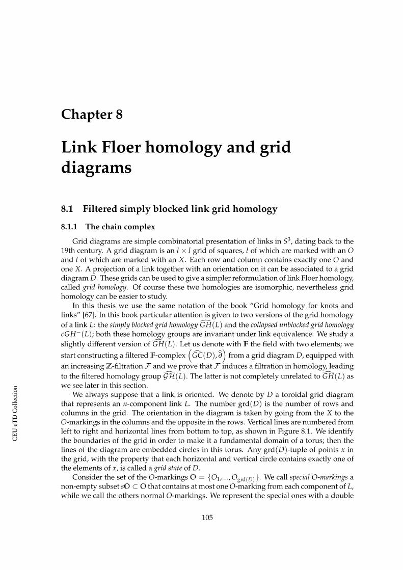
Chapter 8
Link Floer homology and griddiagrams
8.1 Filtered simply blocked link grid homology
8.1.1 The chain complex
Grid diagrams are simple combinatorial presentation of links in S3, dating back to the19th century. A grid diagram is an l × l grid of squares, l of which are marked with an Oand l of which are marked with an X. Each row and column contains exactly one O andone X. A projection of a link together with an orientation on it can be associated to a griddiagram D. These grids can be used to give a simpler reformulation of link Floer homology,called grid homology. Of course these two homologies are isomorphic, nevertheless gridhomology can be easier to study.
In this thesis we use the same notation of the book “Grid homology for knots andlinks” [67]. In this book particular attention is given to two versions of the grid homologyof a link L: the simply blocked grid homology GH(L) and the collapsed unblocked grid homologycGH−(L); both these homology groups are invariant under link equivalence. We study aslightly different version of GH(L). Let us denote with F the field with two elements; westart constructing a filtered F-complex
(GC(D), ∂
)from a grid diagram D, equipped with
an increasing Z-filtration F and we prove that F induces a filtration in homology, leadingto the filtered homology group GH(L). The latter is not completely unrelated to GH(L) aswe see later in this section.
We always suppose that a link is oriented. We denote by D a toroidal grid diagramthat represents an n-component link L. The number grd(D) is the number of rows andcolumns in the grid. The orientation in the diagram is taken by going from the X to theO-markings in the columns and the opposite in the rows. Vertical lines are numbered fromleft to right and horizontal lines from bottom to top, as shown in Figure 8.1. We identifythe boundaries of the grid in order to make it a fundamental domain of a torus; then thelines of the diagram are embedded circles in this torus. Any grd(D)-tuple of points x inthe grid, with the property that each horizontal and vertical circle contains exactly one ofthe elements of x, is called a grid state of D.
Consider the set of the O-markings O = {O1, ..., Ogrd(D)}. We call special O-markings anon-empty subset sO ⊂ O that contains at most one O-marking from each component of L,while we call the others normal O-markings. We represent the special ones with a double
105
CE
UeT
DC
olle
ctio
n

X
X
X
X
X(0, 0)
(0, 5)
(5, 0)
(5, 5)
Figure 8.1: A grid diagram of the positive trefoil knot.
circle in the grid diagram. We usually consider only the case when |sO| = n, which meansthere is exactly one special O-marking on each component. We talk about the general casein Subsection 8.2.2. From now on there are always n special O-markings in a grid diagram,unless it is explicitly written differently.
We define the simply blocked complex GC(D) as the free F[V1, ..., Vgrd(D)−n]-module,where F = Z \ 2Z, over the grid states S(D) = {x1, ..., xgrd(D)!}.
We associate to every grid state x the integer M(x), called the Maslov grading of x,defined as follows:
M(x) = MO(x) = J (x−O, x−O) + 1 ; (8.1)
where
J (P, Q) = ∑a∈P
∣∣∣{(a, b) ∈ (P, Q) | b has both coordinates strictly bigger than
the ones of a}∣∣∣
with coordinates taken in the interval [0, grd(D)).Then we have the Maslov F-splitting
GC(D) =⊕d∈Z
GCd(D)
where GCd(D) is the finite dimensional F-vector space generated by the elements V l11 · ... ·
V lmm x, with x ∈ S(D) and m = grd(D)− n, such that
M(V l11 · ... ·V
lmm x) = M(x)− 2
m
∑i=1
li = d .
We define another integer-valued function on grid states, the Alexander grading A(x), withthe formula
A(x) =M(x)−MX(x)
2− grd(D)− n
2;
where MX(x) is defined in Equation (8.1), replacing the set O with X. For the proof thatA(x) is an integer we refer to [67].
Now we introduce an increasing filtration on GC(D), see Subsection 1.4.1 such that
F sGC(D) =⊕d∈Z
F sGCd(D)
106
CE
UeT
DC
olle
ctio
n

and where F sGCd(D) is generated over F by the elements V l11 · ... ·V
lmm x with Maslov grad-
ing d and Alexander grading
A(V l11 · ... ·V
lmm x) = A(x)−
m
∑i=1
li 6 s .
8.1.2 The differential
First we take x, y ∈ S(D). The set Rect(x, y) is defined in the following way: it is alwaysempty except when x and y differs only by a pair of points, say {a, b} in x and {c, d} iny; then Rect(x, y) consists of the two rectangles in the torus represented by D that havebottom-left and top-right vertices in {a, b} and bottom-right and top-left vertices in {c, d}.We call Rect◦(x, y) ⊂ Rect(x, y) the subset of the rectangles which do not contain a pointof x (or y) in their interior, that are called the empty rectangles.
The differential ∂ is defined as follows:
∂x = ∑y∈S(D)
∑r∈Rect◦(x,y)
r∩sO=∅
VO1(r)1 · ... ·VOm(r)
m y for any x ∈ S(D)
where Oi(r) =
{1 if Oi ∈ r0 if Oi /∈ r
. Here {O1, ..., Om} is the set of the m = grd(D)− n normal
O-markings.We extend ∂ to GCd(D) linearly, and we call it ∂d, then again to the whole GC(D) in
the following way: ∂(Vix) = Vi · ∂x for every i = 1, ..., m and x ∈ S(D). Since ∂ keeps thefiltration and drops the Maslov grading by 1, see [67], we have maps
∂d,s : F sGCd(D) −→ F sGCd−1(D)
where ∂d,s is the restriction of ∂d to the subspace F sGCd(D) ⊂ GCd(D). Furthermore, wehave ∂ ◦ ∂ = 0, see [67] fo more details.
8.1.3 The homology
We define the homology group GHd(D) as the quotient spaceKer ∂d
Im ∂d+1. Moreover, we
introduce the subspaces F sGHd(D) as in Subsection 1.4.1: consider the projection πd :Ker ∂d → GHd(D). Since Ker ∂d,s = Ker ∂d ∩ F sGCd(D) we say that
F sGHd(D) = πd(Ker ∂d,s)
for every s ∈ Z. Ker ∂d,s ⊂ Ker ∂d,s+1 implies that the filtration F descends to homology.We see immediately that each F sGHd(D) is a finite dimensional F-vector space.
We can extend the filtration F on the total homology
GH(D) =⊕d∈Z
GHd(D)
by takingF sGH(D) =
⊕d∈Z
F sGHd(D) .
107
CE
UeT
DC
olle
ctio
n

From [67] we know that the dimension of F sGHd(D) as an F-vector space is a linkinvariant for every d, s ∈ Z, in particular it is independent of the choice of the special O-markings and the ordering of the markings. Hence we can denote them with F sGHd(L).Furthermore, [67] also tells us that [Vi p] = [0] for every i = 1, ..., m and [p] ∈ GH(L). Thismeans that each homology class can be represented by a combination of grid states andevery level F sGH(L) is also a finite dimensional F-vector space.
The homology group GHd,s(L) of [67] can be recovered from the complex GC(D) in thefollowing way. We denote the graded object associated to a filtered complex C, defined inSubsection 1.4.1, as
(gr(C), gr(∂)
). Then we have that
GHd,s(L) ∼=F Hd,s
(gr(
GC(D))
, gr(∂))
.
8.1.4 Equivalence between GH and HFL
We want to show that the chain complex(
GC(D), ∂1
), obtained from a grid diagram D
which represents the link L, can be identified with the chain complex(
CFL(H), ∂2
)given
by an appropriate Heegaard diagram H.Let HD be the (unbalanced) multi-pointed Heegaard diagram (Σ, α, β, w, z), see Sub-
section 4.1.2, defined as follows. The surface Σ is the torus which is given by D; in fact,in Subsection 8.1.1 we defined D precisely as a square representing the fundamental do-main of a torus. The curves α and β correspond one-to-one with the horizontal and verticalcurves in D. Finally, we take the O-markings as the set of basepoints w and the X-markingsas z. Then we have the following theorem.
Theorem 8.1.1 There is an isomorphism of chain complexes
Ξ : GC(D) −→ CFL(HD)
which preserves the bigradings.
Proof. We give an idea of the proof, which can be found in [67]. First, we observe that gridstates in D correspond to the intersction points in HD. Now suppose that φ ∈ π2(x, y) issuch that its associated domain in D belongs to Rect◦(x, y). Then we have that µ(φ) = 1and
∣∣∣M(φ)∣∣∣ = 1. This is verified using the following interpretation of holomorphic disks
in the symmetric product. A holomorphic disk in Symd(Σ) can be viewed as the followingcollection (F, P, f ) of data:
1. a surface with boundary F, equipped with a complex structure;
2. a degree d holomorphic map P : F → D, where D is the standard disk in C;
3. a holomorphic map f : F → Σ.
In this correspondence, the domain of the holomorphic disk can be thought of as the two-chain induced by the map f from F to Σ. Then the claim follows from the Riemann map-ping theorem. See [67] for more details.
108
CE
UeT
DC
olle
ctio
n

We say that a domain is called positive if its local multiplicities are all non-negative,and at least one of them is positive. Let ψ ∈ π2(x, y) be a positive domain. Then, thereis a sequence of grid states {x1, ..., xk}, with x1 = x and xk = y, and empty rectangles{ri, ..., rk−1}, with ri ∈ Rect◦(x1, xi+1) for i = 1, ..., k− 1, so that ψ = r1 ∗ ... ∗ rk−1. The proofof this fact is also given in [67].
At this point, we can identify the boundary maps as follows. As we said in Chapter 5, ifa domain φ is associated to a holomorphic strip then it has non-negative local multiplicitieseverywhere. Domains with zero local multiplicities everywhere correspond to constantmaps, which have µ(φ) = 0, and so they are not counted in the differential. Any othersuch domain φ can be factored as φ = φ1 ∗ ... ∗ φm, where each φi is an empty rectangle.
Since µ is additive under composition, and µ(φi) = 1 for what we said before, weconclude that µ(φ) = m. Since the holomorphic strips counted in the differential haveMaslov index one, we conclude that only empty rectangles are counted in the differential.Moreover, each such rectangle really appears in the differential from the first obervation,completing the identification of ∂2 with ∂1.
Since the Maslov and Alexander gradings transform the same in both theories, whenφ corresponds to an empty rectangle, it follows that the the identification of complexesrespects relative bigradings. In fact, the identification respects absolute bigradings, sincein both theories, the Alexander grading is normalized to be symmetric, and the Maslovgrading is normalized using the total homology of the complexes.
In particular, this means that the simply blocked grid homology group GH(L) is iso-morphic to HFL(L) as bigraded F-vector spaces. In light of this, from now on in thischapter we always write HFL(L) for the homology of the chain complex
(GC(D), ∂1
).
Furthermore, we denote with HFL(L) the filtered homology group GH(L) introducedin Subsection 8.1.3.
8.2 The invariant tau in the filtered theory
8.2.1 Definition of the invariant
Since F s−1HFLd(L) ⊂ F sHFLd(L), and they are finite dimensional vector spaces,we define the function
TL(d, s) = dimF
F sHFLd(L)
F s−1HFLd(L)
which clearly is still a link invariant.Our first goal is to see what happens to this function T when we stabilize the link L, in
other words when we add a disjoint unknot to L. Denote the unknot with the symbol©.We claim that
TLt©(d, s) = TL(d, s) + TL(d + 1, s) for any d, s ∈ Z . (8.2)
We refer to Subsection 1.4.2 before for some remarks on filtered chain maps. Moreover,we define the shifted complex C [[ a, b ]] = C ′ as F sC ′d = F s−bCd−a. Now, in order to proveEquation (8.2), we need the following proposition.
109
CE
UeT
DC
olle
ctio
n

Proposition 8.2.1 For any link L we have HFL(L t©) ∼= HFL(L)⊗ V, where V is the twodimensional F-vector space with generators in grading and minimal level (d, s) = (−1, 0) and(d, s) = (0, 0).
Proof. Take a grid diagram D for L. Then the extended diagram D, obtained from D byadding one column on the left and one row on the top with a doubly-marked square in thetop left, represents the link L t©. The circle in the doubly-marked square is forced to bea special O-marking and we can also suppose that there is another special O-marking justbelow and right of it, as shown in Figure 8.2.
X z
Figure 8.2: We call the top-left special O-marking O0.
Let I(D) denote the set of those generators in S(D) which have a component at thelower-right corner of the doubly-marked square, and let N(D) be the complement of I(D)in S(D). From the placement of the special O-markings, we see that N(D) spans a sub-complex N in GC(D). Moreover, if ∂1 is the differential in GC(D) and ∂2 the one in GC(D)
we can express the restriction of ∂1 to the subspace I, spanned by I(D), with ∂2 + ∂N; thisbecause there is a one-to-one correspondence between elements of I(D) and grid states inS(D). This correspondence induces a filtered quasi-isomorphism i : (I, ∂2)→ GC(D).
Define a map H : N→ I by the formula
H(x) = ∑y∈I(D)
∑r∈Rect◦(x,y)
O0∈r
VO1(r)1 · ... ·VOm(r)
m y for any x ∈ N(D) .
We have that H is a filtered chain homotopy equivalence between (N, ∂1) and (I, ∂2), whichincreases the Maslov grading by one, and H ◦ ∂N = 0. To see the first claim, we mark thesquare just on the right of O0 with z and we define an operator Hz : I → N, which countsonly rectangles that contain z. This operator is a homology inverse of H; this and thesecond claim can be proved in the same way as in [67]. Those two facts together tell usthat the following diagram commutes.
I N
GC(D) GC(D) [[−1, 0 ]]
∂N
i i ◦ H
0
Since H is a filtered chain homotopy equivalence, i ◦ H is a filtered quasi-isomorphism,just like the map i. Therefore, we can use Lemma 1.4.4 and obtain that the map between
110
CE
UeT
DC
olle
ctio
n

the mapping cones
Cone(∂N) = GC(D) −→ Cone(0) = GC(D)⊗V
is a filtered quasi-isomorphism and so the claim follows easily from Propositions 1.4.1 and1.4.3. See also [67] for more details.
Equation (8.2) is obtained immediately from Proposition 8.2.1, in fact we have provedthat F sHFLd(L t ©) ∼= F sHFLd(L) ⊕ F sHFLd+1(L) for every d, s ∈ Z and so it isenough to apply the definition of T.
Now we are able to do some computations. The homology of the unknot can be easilycomputed by taking the grid diagram of dimension one, where the square is marked withboth X and O. The complex has one element of Maslov and Alexander grading 0; thenT©(d, s) = 1 if (d, s) = (0, 0) and it is 0 otherwise.
Using Equation (8.2) we get the function T of the n-component unlink©n:
T©n(d, s) =
(
n− 1k
)if (d, s) = (−k, 0), 0 6 k 6 n− 1
0 otherwise.
We can also see this directly from Proposition 8.2.1, in fact we have that HFL(©n) ∼=V⊗(n−1).
Now let us consider a grid diagram D of a link L. The Maslov grading of the elementsof S(D) and the differential ∂ are independent of the position of the X’s, once we havefixed the special O-markings. Since we can always change the X-markings to obtain©n,this means that dimFHFLd(L) = dimFHFLd(©n) for every d ∈ Z and the generatorsare the same. In particular
HFL(L) ∼=F HFL(©n) ∼=F F2n−1and HFLd(L) ∼=F F(n−1
−d ) when 1− n 6 d 6 0 .
From this we have that HFL0(L) has always dimension one and then we define τ(L)as the only integer s such that TL(0, s) > 0. We remark that for a knot this version of τcoincides with the one of Ozsváth and Szabó. See the proof of Theorem 8.4.1 in Section 8.4.We also observe that Equation (8.2) tells that τ(L t©) = τ(L).
8.2.2 Dropping the special O-markings
In this subsection we study what happens to the homology of the filtered chain com-plex
(GC(D), ∂
)if the grid diagram D has less than n special O-markings.
Let us consider D a grid diagram for an n-component link L. The set sO ⊂ O containsat most one O-marking from each component of L, but we have that |sO| > 1. Denotewith m = grd(D)− |sO| the number of normal O-markings in D. Then we can define ourchain complex exactly in the same way as in Section 8.1; on the other hand, the homologyGH(D) is no longer a link invariant, in fact it clearly depends of the choice of the specialO-markings.
Nonetheless, we can show that the F-vector space GH(D) is still finite dimensional.Note that this is not true if instead we consider the bigraded simply blocked grid homologygroup GH(D).
111
CE
UeT
DC
olle
ctio
n

Proposition 8.2.2 The homology group GH(D), defined as in Subsection 8.1.3, is F-isomorphicto GH
(©|sO|
), the homology of the unlink with |sO| components each containing a special O-
marking. In particular, we have that
GH(D) ∼=F F2|sO|−1 and GHd(D) ∼=F F(|sO|−1−d )
when 1− |sO| 6 d 6 0.
Proof. As we noted before, the group GH(D) does not depend on the position of the X-marking. Since we can always change them in a way that D becomes a diagram for anunlink with a special O-marking on every component, the claim follows from the resultsin the previous subsection.
Even though in this case the homology is no longer a link invariant, we can still provethe following theorem.
Theorem 8.2.3 Let us consider two grid diagrams D1 and D2 representing smoothly isotopic linksL1 and L2 such that all the isotopic components both contain or not contain a special O-marking.Then we have that GH(D1) is filtered isomorphic to GH(D2) and the isomorphism preserves theMaslov grading.
Proof. From [82] we know that such two grid diagrams differ by a finite sequence of gridmoves: reordering of the O-markings, commutations and stabilizations. Then it is enoughto prove the theorem in the case when D2 is obtained from D1 by one of these three moves.
The maps that we defined in Chapter 5 can be arranged to give filtered quasi-isomorphisms for each move. This implies that GH(D1) ∼= GH(D2). See also the results in[67] to find the maps in the grids setting.
Hence, we can denote the homology group of an n-component link L with GHO(L)
and it depends only on which components of the link contain a special O-marking. We use
the homology groups GHO(L) to define some cobordism maps in Section 8.3.
8.2.3 Symmetries
Reversing the orientation
If −L is the link obtained from L by reversing the orientation of all the componentsthen
T−L(d, s) = TL(d, s) for any d, s ∈ Z (8.3)
and τ(−L) = τ(L).To see this, consider a grid diagram D of L, then it is easy to observe that, if we reflect
D along the diagonal going from the top-left to the bottom-right of the grid, the diagramD′ obtained in this way represents −L. Hence, we take the map Φ : S(D) → S(D′) thatsends a grid state x into its reflection x− and now, from [67], we have that M(x−) = M(x)and A(x−) = A(x). This means that Φ is a filtered quasi-isomorphism between GC(D)
and GC(D′), since clearly the differentials commute with Φ.This gives another proof that HFL(−L) ∼= HFL(L) and then Equation (8.3) follows.
112
CE
UeT
DC
olle
ctio
n

Mirror image
For an n-component link L we have that the function T of the mirror image L∗ is givenby the following equation
TL∗(d, s) = TL(−d + 1− n,−s) for any d, s ∈ Z . (8.4)
To see this, we first, given a complex C with a filtration F , introduce the filtered dualcomplex C∗, equipped with a filtration F ∗ by taking
(F ∗)s(C∗)d = Ann(F−s−1C−d) ⊂ (C−d)∗ = (C∗)d for any d, s ∈ Z ,
where Ann(F hCk) is the subspace of (Ck)∗ consisting of all the linear functionals that are
zero over F hCk.Second, given a grid diagram D of L, we call
(GC(D), ∂
)the filtered chain complex(
GC(D), ∂)
V1 = ... = Vm = 0and we also denote with W the two dimensional F-vector space with
generators in grading and minimal level (d, s) = (0, 0) and (d, s) = (−1,−1).
Lemma 8.2.4 We have the filtered quasi-isomorphism
GC(D) ∼= GC(D)⊗W⊗(grd(D)−n) , (8.5)
where D is a grid diagram for an n-component link L.
Proof. Suppose that V1 and V2 are variables which belong to the same component of L.Then it follows from [67, Lemma 14.1.11] that
GC(D)
V1 = V2
∼= GC(D)⊗W .
Therefore, we conclude by iterating this procedure.
We want to prove the following proposition.
Proposition 8.2.5 HFL(L∗) ∼= HFL∗(L)J1− n, 0K, where the filtration on HFL
∗(L) is F ∗.
Proof. Let D∗ be the diagram obtained by reflecting D through a horizontal axis. The di-agram D∗ represents L∗. Reflection induces a bijection x → x∗ between grid states for Dand those for D∗, inducing a bijection between empty rectangles in Rect◦(x, y) and emptyrectangles in Rect◦(y∗, x∗). Hence, the reflection induces a filtered isomorphism
GC(D∗) ∼= GC∗(D) [[ 1− grd(D), n− grd(D) ]] ,
where the shifts are given by the fact that M(x∗) = −M(x) + 1− grd(D) and A(x∗) =−A(x) + n− grd(D).
Now Lemma 8.2.4 and observing that
(W∗)⊗(grd(D)−n) ∼= W⊗(grd(D)−n) [[ grd(D)− n, grd(D)− n ]]
lead to the filtered quasi-isomorphism
GC(D∗) ∼= GC∗(D) [[ 1− n, 0 ]] .
113
CE
UeT
DC
olle
ctio
n

Proposition 8.2.5 says thatF sHFLd(L∗) ∼= (F ∗)s(HFL
∗)d−1+n
(L) for every d, s ∈ Z.
Then we can prove Equation (8.4):
TL∗(d, s) = dim(F ∗)s
(HFL
∗)d−1+n
(L)
(F ∗)s−1(HFL
∗)d−1+n
(L)= dim
Ann(F−s−1HFL−d+1−n(L)
)Ann
(F−sHFL−d+1−n(L)
) =
= dimF−sHFL−d+1−n(L)
F−s−1HFL−d+1−n(L)= TL(−d + 1− n,−s) .
If we define τ∗(L) as the unique integer such that TL(1 − n, τ∗(L)) = 1 then we haveproved that
τ(L∗) = −τ∗(L) . (8.6)
In particular for a knot K, where τ∗(K) = τ(K), we have τ(K∗) = −τ(K). Moreover, wehave the following corollary.
Corollary 8.2.6 Suppose that L is smoothly isotopic to L∗. Then,
TL∗(d, s) = TL(d, s) for any d, s ∈ Z
and so Equation (8.4) gives that the function TL has a central symmetry in the point( 1−n
2 , 0). In
particular τ∗(L) = −τ(L) and, for knots, τ(K) = 0.
Connected sum
Given two links L1 and L2, the function T of the connected sum L1# L2 is the convolu-tion product of the T functions of L1 and L2; in other words
TL1# L2(d, s) = ∑d=d1+d2s=s1+s2
TL1(d1, s1) · TL2(d2, s2) for any d, s ∈ Z . (8.7)
This equation is very hard to prove in the grid diagram settings, but it can be proved usingthe holomorphic definition of link Floer Homology, as we saw in Subsection 6.6.1. See also[72].
We see immediately that the homology and the T function of L1# L2 are independentof the choice of the components used to perform the connected sum; moreover, the τ-invariant is additive:
τ(L1# L2) = τ(L1) + τ(L2) .
Disjoint union
The disjoint union of two links L1 and L2 is equivalent to L1# (L2 t©). Thus by Equa-tions (8.2) and (8.7) we have the following relation:
TL1tL2(d, s) = ∑d=d1+d2s=s1+s2
TL1(d1, s1) ·(TL2(d2, s2) + TL2(d2 + 1, s2)
)for any d, s ∈ Z , (8.8)
or in other words HFL(L1 t L2) ∼= HFL(L1) ⊗ HFL(L2) ⊗ V, where V is the two di-mensional F-vector space with generators in grading and minimal level (d, s) = (−1, 0)and (d, s) = (0, 0). We have immediately that
τ(L1 t L2) = τ(L1# L2) = τ(L1) + τ(L2) .
114
CE
UeT
DC
olle
ctio
n

Quasi-alternating links
We recall that quasi-alternating links are the smallest set of links Q that satisfies thetwo properties:
1. the unknot is in Q;
2. L is in Q if it admits a diagram with a crossing whose two resolutions L0 and L1 areboth in Q, det(Li) 6= 0 and det(L0) + det(L1) = det(L).
The above definition and a result in [71] imply that every quasi-alternating link is non-splitand every non-split alternating link is quasi-alternating. Moreover, quasi-alternating linksare both Khovanov and link Floer homology thin, which means that their homologies aresupported in two and one lines respectively, and the homology is completely determinedby the signature and the Jones (Alexander in the hat version of link Floer homology) poly-nomial. The following proposition says that the same is true in filtered grid homology.
Theorem 8.2.7 If L is an n-component quasi-alternating link then the function TL is supported ina line; more specifically the following relation holds:
TL(d, s) 6= 0 if and only if s = d +n− 1− σ(L)
2for 1− n 6 d 6 0
where σ(L) is the signature of L.
Proof. We already know that if TL(d, s) 6= 0 then 1− n 6 d 6 0, so we only have to provethe alignment part of the statement.
Take a grid diagram D for L, then from [67] the claim is true for the bigradedhomology of
(gr(
GC(D))
, gr(∂))∼= HFL(L). Since TL(d, s) 6= 0 implies that
Hd,s
(gr(
GC(D))
, gr(∂))
is non-zero, the theorem follows.
From Theorem 8.2.7 we obtain immediately the following corollary.
Corollary 8.2.8 If L is an n-component quasi-alternating link then τ(L) = n−1−σ(L)2 and τ(L∗) =
n− 1− τ(L).
8.3 Cobordisms
8.3.1 Induced maps and degree shift
In this section we study the behaviour of the function T under cobordisms, see Section1.3. Some of the induced maps that appear in this subsection come from the work of Sarkarin [82]; though the grading shifts are different, because Sarkar used a different definitionof the Alexander grading, ignoring the number of component of the link.
It is a standard result in Morse theory that a link cobordism can be decomposed intofive standard cobordisms. We find maps in homology for each case. From now on, givena link Li, we denote with Di one of its grid diagrams.
115
CE
UeT
DC
olle
ctio
n

L1 L2
Figure 8.3: Identity cobordism.
i) Identity cobordism. This cobordism, with no critical points (Figure 8.3), represents asequence of Reidemeister moves; in other words L1 and L2 are smoothly isotopic.At the end of Section 8.1 we remarked that filtered homology is a link invariant; moreprecisely what we have is a filtered quasi-isomorphism between GC(D1) and GC(D2).This, as we know, induces a filtered isomorphism in homology.
ii) Split cobordism. This cobordism (right in Figure 8.4) represents a band move when L2has one more component than L1. Take D1 with a 2× 2 square with two X-markings,one at the top-left and one at the bottom-right; then we claim that D2 is obtained fromD1 by deleting this two X-markings and putting two new ones: at the top-right andthe bottom-left, as shown in Figure 8.5. In order to construct the complex GC(D2) we
L1 L2 L1 L2
Figure 8.4: Merge and split cobordisms.
need to create one more special O-marking on the new component of L2. To avoid thisproblem we first consider the identity map in the filtered GC theory
Id : GC(D1) −→ GC(D2) ,
which clearly is a chain map since now every O-marking is special; moreover, it in-duces an isomorphism in homology, that preserves the Maslov grading, and a directcomputation gives that it is filtered of degree one.
Now we use Equation (8.5) and we get an isomorphism
ΦSplit : HFL(L1)⊗W −→ HFL(L2)
that is a degree one filtered map which still preserves the Maslov grading. The W
116
CE
UeT
DC
olle
ctio
n

X
X
X
X
Figure 8.5: Band move in a grid diagram.
factor appears because in Equation (8.5) we take into account the size of Di and thenumber of components of Li; while the first quantity is the same for both diagramsthe link L2 has one more component than L1.
iii) Merge cobordism. This cobordism (left in Figure 8.4) represents a band move when L1has one more component than L2. We have an isomorphism
ΦMerge : HFL(L1) −→ HFL(L2)⊗W .
The map is obtained in the same way as ΦSplit in the previous case, but with the dif-ference that now it is filtered of degree zero.
L1 L2
Figure 8.6: Torus cobordism.
Sometimes we are more interested in when a split and a merge cobordism appear together,the second just after the first, in the shape of what we call a torus cobordism (Figure 8.6).We have the following proposition.
Proposition 8.3.1 Let Σ be a torus cobordism between two links L1 and L2. Then Σ induces aMaslov grading preserving isomorphism between HFL(L1) and HFL(L2), which is filtered ofdegree one.
Proof. We can choose D1 in a way that the split and the merge band moves can be per-formed on two disjoint bands. Then we apply twice the move shown in Figure 8.5 and wetake as map the identity. In this case the identity is a chain map because L2 has the samenumber of components of L1; this means that the special O-markings in D1 and D2 are the
117
CE
UeT
DC
olle
ctio
n

L2
L1
Figure 8.7: Birth cobordism.
same and then the two differentials coincide. In this way we obtain an isomorphism inhomology with Maslov grading shift and filtered degree equal to the sum of the ones in ii)and iii).
iv) Birth cobordism. A cobordism (Figure 8.7) representing a birth move.
Since our cobordisms have boundary in both L1 and L2, we can always assume that a birthmove is followed (possibly after some Reidemeister moves) by a merge move. Thus it isenough to define a map for the composition of these three cobordisms and this is what wedo in the following proposition.
Proposition 8.3.2 Let Σ be a cobordism between two links L1 and L2 like the one in Figure8.8. Then Σ induces an isomorphism ΦBirth between HFL(L1) and HFL(L2) that preservesthe Maslov grading and it is filtered of degree zero.
L2
L1
Figure 8.8: A more useful birth cobordism.
Proof. The first step is to construct a map s1 associated to the grid move shown in Figure8.9; note that we add a normal O-marking, since later we merge the new unknot compo-nent with an already exisiting one. Let us denote with D′1 the stabilized diagram and withc = α∩ β the point in the picture; then we have the inclusion i : S(D1)→ S(D′1) that sendsa grid state x in D1 to the grid state in D′1 constructed from x by adding the point c. Thens1 : GC(D1)→ GC(D′1) is defined by the following formula:
s1(x) = ∑y∈S(D′1)
∑H∈SL(i(x),y,c)
H∩sO=∅
Vn1(H)1 · ... ·Vnm(H)
m y for any x ∈ S(D1)
where SL(x, z, p) is the set of all the snail-like domains, the exact definition can be found
118
CE
UeT
DC
olle
ctio
n

D1D1
Xα
β
c
Figure 8.9: Birth move in a grid diagram.
in [67], centered at p joining x to z, illustrated in Figure 8.10; ni(H) is the number of timesH passes through Oi and m is the number of the normal O-markings of D1. In [58] isproved that s1 is a filtered quasi-isomorphism which induces a filtered isomorphism be-
tween HFL(L1) → GHO(L1 t©); where the special O-markings on L1 t © coincide
with the ones on L1 (the new unknotted component has a normal O-marking). Moreover,in [82] Sarkar showed that the map s1 is filtered of degree zero.
At this point we compose s1 with the map s2 given by the Reidemeister moves, which isa filtered quasi-isomorphism by Theorem 8.2.3, and finally with s3, the identity associated
to the band move of Figure 8.5. The map s3 induces an isomorphism GHO(L1 t©) →
Figure 8.10: Some of the snail-like domains SL(x, z, p): the coordinates of x and z arerepresented by the white and black circles.
HFL(L2) that clearly preserves the Maslov grading and again we easy compute that it isfiltered of degree zero.
Hence, the composition of these three maps induces the isomorphism in the claim.
v) Death cobordism. This cobordism (Figure 8.11) represents a death move. Since this movecan also be seen as a birth move between L∗2 and L∗1 , we take the dual map of
ΦBirth : HFL(L∗2) −→ HFL(L∗1)
which exists from Proposition 8.3.2; then Φ∗Birth = ΦDeath, by Proposition 8.2.5, is amap between HFL(L1) and HFL(L2). Furthermore, it is still an isomorphism that isfiltered of degree zero and preserves the Maslov grading.
The results for birth and death cobordisms in this section immediately give the followingcorollary.
Corollary 8.3.3 Suppose there is a birth or a death cobordism as in Figures 8.8 and 8.11 betweentwo links L1 and L2. Then we have that HFL(L1) ∼= HFL(L2).
119
CE
UeT
DC
olle
ctio
n

L2
L1
Figure 8.11: Death cobordism.
8.3.2 Strong concordance invariance
We remark that a strong cobordism is a cobordism Σ, between two links with the samenumber of components, such that every connected component of Σ is a knot cobordism be-tween a component of the first link and one of the second link. Moreover, if the connectedcomponents of Σ are all annuli then we call Σ a strong concordance, see Section 1.3. Wewant to prove the following theorem.
Theorem 8.3.4 The function T is a strong concordance invariant. In other words, if L1 and L2 arestrongly concordant then TL1(d, s) = TL2(d, s) for every d, s ∈ Z.
We start by observing that Proposition 8.3.1 leads to the following corollary.
Corollary 8.3.5 Suppose there is a strong cobordism Σ between L1 and L2 such that Σ is thecomposition of g(Σ) torus cobordisms, not necessarily all of them belonging to the same componentof Σ. Then Σ induces an isomorphism between HFL(L1) and HFL(L2), which is filtered ofdegree g(Σ) and preserves the Maslov grading.
Now, if we have an isomorphism F : HFL(L1) → HFL(L2) that preserves theMaslov grading and it is filtered of degree t, which means that there are inclusionsF(F sHFLd(L1)
)⊂ F s+tHFLd(L2) for every d, s ∈ Z, then τ(L2) 6 τ(L1) + t. Hence,
we can prove the following theorem that immediately implies the invariance statement.
Theorem 8.3.6 Suppose that Σ is a strong cobordism between two links L1 and L2. Then∣∣τ(L1)− τ(L2)∣∣ 6 g(Σ) .
Furthermore, if L1 and L2 are strongly concordant then HFL(L1) ∼= HFL(L2).
Proof. From [67] we can suppose that, in Σ, 0-handles come before 1-handles while 2-handles come later; moreover, we can say that Σ is the composition of birth, torus anddeath cobordisms (and obviously some identity cobordisms). Each of these induces anisomorphism in homology that also respects the Maslov grading.
For the first part, we only need to check what is the filtered degree of the isomorphismbetween HFL(L1) and HFL(L2), obtained by the composition of all the induced maps oneach piece of Σ. Birth, death and identity are filtered of degree zero, while, from Corollary8.3.5, the torus cobordisms are filtered of degree g(Σ). Then we obtain
τ(L2) 6 τ(L1) + g(Σ) .
For the other inequality we consider the same cobordism, but this time from L2 to L1.Now, for the second part, we observe that now there are no torus cobordisms and then
the claim follows from Corollary 8.3.3.
120
CE
UeT
DC
olle
ctio
n

8.3.3 A lower bound for the slice genus
Suppose Σ is a cobordism (not necessarily strong) between two links L1 and L2. Denotewith Σ1, ..., ΣJ the connected components of Σ. For i = 1, 2 we define the integers lk
i (Σ) asthe number of components of Li that belong to Σk minus 1; in particular lk
i (Σ) > 0 for any
k, i. Finally, we say that li(Σ) =J
∑k=1
lki (Σ) = ni − J, where ni is the number of component
of Li. For example, if Σ is the cobordism in Figure 8.12 then J = 2, ordering Σ1 and Σ2from above to bottom, we have that l1(Σ) = 3 and l2(Σ) = 4; while l1
1(Σ) = 2, l21(Σ) = 1,
l12(Σ) = 3 and l2
2(Σ) = 1. We have the following lemma.
Lemma 8.3.7 If Σ has no 0,2-handles then, up to rearranging 1-handles, we can suppose that Σis like in Figure 8.12: there are l1(Σ) merge cobordisms between (0, t1), l2(Σ) split cobordismsbetween (t2, 1) and g(Σ) torus cobordisms between (t1, t2). We have no other 1-handles except forthe ones we considered before.
t1 t2
L1
L2
0 1
Figure 8.12: An example of a cobordism between two links after rearranging handles.
Proof. We consider a connected component Σk, which is a cobordism between Lk1 and Lk
2,and we fix a Morse function f : S3 × [0, 1] → [0, 1]. After some Reidemeister moves, from[67] we know that we can assume that all the band moves are performed on disjoint bands,in particular we can apply them in every possible order.
Since Σk has boundary in both Lk1 and Lk
2 by the definition of cobordism given at begin-ning of Section 1.3, if we take an ordering for the components of Lk
1, we can find a mergecobordism joining the first and the second component of Lk
1 at some point t in (0, 1); weassume that the associated band move is the first we apply on Lk
1. Now we just do the samething on the other components, but taking the new component instead of the first two. Inthis way we have that there is a t1 ∈ (0, 1) such that Σk ∩ f−1[0, t1] is composed by lk
1(Σ)merge cobordisms and Σk ∩ f−1(t1) is a knot.
In the same way we find that, for a certain t2 ∈ (0, 1), the cobordism Σk ∩ f−1[t2, 1] iscomposed by lk
2(Σ) split cobordisms and Σk ∩ f−1(t2) is a knot.
121
CE
UeT
DC
olle
ctio
n

At this point Σk ∩ f−1[t1, t2] is a knot cobordism of genus g(Σk) and from [67], see also[51], we can rearrange the saddles to obtain a composition of g(Σk) torus cobordisms likein Figure 8.12.
To see that there are no other 1-handles left it is enough to compute the Euler charac-teristic of Σk:
2− 2g(Σk)− lk1(Σ)− 1− lk
2(Σ)− 1 = χ(Σk) = −|1-handles| .
This means that the number of 1-handles in Σk is precisely 2g(Σk) + lk1(Σ) + lk
2(Σ).
From Figure 8.12 we realize that merge and split cobordisms can appear alone in Σand not always in pair like in strong cobordisms. In case ii) and iii) of Subsection 8.3.1we see that they do not induce isomorphisms in homology, but we find maps ΦSplit and
ΦMerge that are indeed isomorphisms if restricted to HFL0(L1) → HFL0(L2); moreover,the filtered degree is one for split cobordisms and zero for merge cobordisms. Since weare looking for information on τ, this is enough for our goal and then we can prove thefollowing inequality.
Proposition 8.3.8 Suppose Σ is a cobordism between two links L1 and L2. Then∣∣τ(L1)− τ(L2)∣∣ 6 g(Σ) + max {l1(Σ), l2(Σ)} .
Proof. From Corollary 8.3.3 and Theorem 8.3.6, we can suppose that there are no 0 and no2-handles in Σ. We can also assume that Σ is like in Lemma 8.3.7.
All of these cobordisms induce isomorphisms of the homology in Maslov grading zero.The number of torus cobordisms is g(Σ) while the number of split cobordisms (that are notpart of torus cobordisms) is l2(Σ). This means that
τ(L2) 6 τ(L1) + g(Σ) + l2(Σ) .
Now we do the same, but considering the cobordism going from L2 to L1, as we did in theproof of Theorem 8.3.6. We obtain that
τ(L1) 6 τ(L2) + g(Σ) + l1(Σ) .
Putting the two inequalities together proves the relation in the statement of the theorem.
If L is an n-component link, from Proposition 8.3.8 we have immediately that
|τ(L)|+ 1− n 6 g4(L) (8.9)
which, as we already said, is a lower bound for the slice genus of our link. Indeed, we cansay more by using Equation (8.6) and observing that g4(L∗) = g4(L):
max{|τ(L)|, |τ∗(L)|
}+ 1− n 6 g4(L) .
122
CE
UeT
DC
olle
ctio
n
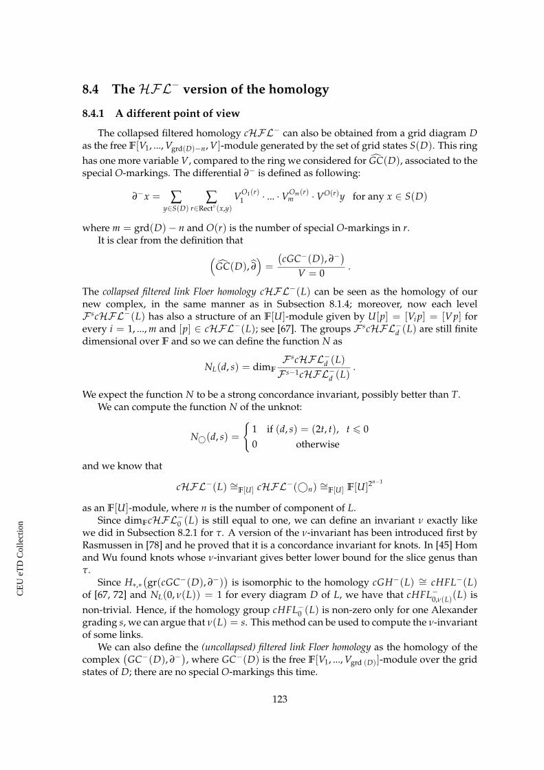
8.4 TheHFL− version of the homology
8.4.1 A different point of view
The collapsed filtered homology cHFL− can also be obtained from a grid diagram Das the free F[V1, ..., Vgrd(D)−n, V]-module generated by the set of grid states S(D). This ringhas one more variable V, compared to the ring we considered for GC(D), associated to thespecial O-markings. The differential ∂− is defined as following:
∂−x = ∑y∈S(D)
∑r∈Rect◦(x,y)
VO1(r)1 · ... ·VOm(r)
m ·VO(r)y for any x ∈ S(D)
where m = grd(D)− n and O(r) is the number of special O-markings in r.It is clear from the definition that(
GC(D), ∂)=
(cGC−(D), ∂−
)V = 0
.
The collapsed filtered link Floer homology cHFL−(L) can be seen as the homology of ournew complex, in the same manner as in Subsection 8.1.4; moreover, now each levelF scHFL−(L) has also a structure of an F[U]-module given by U[p] = [Vi p] = [Vp] forevery i = 1, ..., m and [p] ∈ cHFL−(L); see [67]. The groups F scHFL−d (L) are still finitedimensional over F and so we can define the function N as
NL(d, s) = dimF
F scHFL−d (L)F s−1cHFL−d (L)
.
We expect the function N to be a strong concordance invariant, possibly better than T.We can compute the function N of the unknot:
N©(d, s) =
{1 if (d, s) = (2t, t), t 6 00 otherwise
and we know that
cHFL−(L) ∼=F[U] cHFL−(©n) ∼=F[U] F[U]2n−1
as an F[U]-module, where n is the number of component of L.Since dimFcHFL−0 (L) is still equal to one, we can define an invariant ν exactly like
we did in Subsection 8.2.1 for τ. A version of the ν-invariant has been introduced first byRasmussen in [78] and he proved that it is a concordance invariant for knots. In [45] Homand Wu found knots whose ν-invariant gives better lower bound for the slice genus thanτ.
Since H∗,∗(gr(cGC−(D), ∂−)
)is isomorphic to the homology cGH−(L) ∼= cHFL−(L)
of [67, 72] and NL(0, ν(L)) = 1 for every diagram D of L, we have that cHFL−0,ν(L)(L) isnon-trivial. Hence, if the homology group cHFL−0 (L) is non-zero only for one Alexandergrading s, we can argue that ν(L) = s. This method can be used to compute the ν-invariantof some links.
We can also define the (uncollapsed) filtered link Floer homology as the homology of thecomplex
(GC−(D), ∂−
), where GC−(D) is the free F[V1, ..., Vgrd (D)]-module over the grid
states of D; there are no special O-markings this time.
123
CE
UeT
DC
olle
ctio
n

We see immediately that for every n-component link L is
HFL−(L) ∼= F[U1, ..., Un]
with generator in Maslov grading zero, but the filtration will of course depend on L.
8.4.2 Filtered link homology and the τ-set
In this subsection we prove the following theorem.
Theorem 8.4.1 For an n-component link the τ-set, defined in [67] as -1 times the Alexander grad-ings of a homogeneous, free generating set of the torsion-free quotient of cHFL−(L) as an F[U]-module, coincides with the 2n−1 (with multiplicity) values of s where the function T is supported.
Proof. We use the complex cGC− to show that, for every n-component link L, an integers gives Td,s(L) 6= 0 for some d if and only if s belongs to the τ-set of L. To do this, givenC a freely and finitely generated F[U]-complex, we define two set of integers: τ(C) andt(C). First we call Bτ(C) a homogeneous, free generating set of the torsion-free quotientof H∗,∗ (gr(C)) as an F[U]-module; then τ(C) is the set of s ∈ Z such that there is a [p] ∈Bτ(C) with bigrading (d,−s) for some d ∈ Z. Similarly, t(C) is the set of the integers ssuch that the inclusion
is : F s−1H∗
(C
U = 0
)↪−→ F sH∗
(C
U = 0
)is not surjective. Note that the set Bτ(C) is not unique, but τ(C) and t(C) are well-defined.
We say that s ∈ τ(C) has multiplicity k if there are k distinct elements in Bτ(C) withbigrading (∗,−s), while a number u ∈ t(C) has multiplicity k if Coker iu has dimension kas an F-vector space.
Clearly, if D is a grid diagram of L, t(cGC−(D)
)is the set of the values of s where
the function TL is supported; moreover, we already remarked that H∗,∗ (gr (cGC−(D)))is isomorphic to cHFL−(L) and then τ
(cGC−(D)
)is the τ-set of L. Hence our goal is to
prove that t(cGC−(D)
)= τ
(cGC−(D)
).
Consider the complex
C = cGC−(D)
V1 = ... = Vm = U,
where m = grd(D)− n and U is the variable associated to the special O-markings. Thenwe define C as the complex CJ1− n−m,−mK.
We introduce a new complex C ′ = C ⊗F[U] F[U, U−1] and we define a Z⊕Z-filtrationon C ′ in the following way: F x,∗C ′ = U−xC for every x ∈ Z, F ∗,yC ′ = F yC ′ =
{p ∈
C ′ | A(p) 6 y}
for every y ∈ Z and F x,yC ′ = F x,∗C ′ ∩ F ∗,yC ′ = U−xF y−xC for everyx, y ∈ Z. The first step is to prove that τ(C) = t(C).
We have thatC
U = 0∼= GC(D) ∼=
F 0,∗C ′F−1,∗C ′ ;
moreover, for every integer s we claim that
F sGC(D) ∼=F 0,sC ′F−1,sC ′ .
124
CE
UeT
DC
olle
ctio
n

Since, from [67], it is F x,yC ′ ∼= F y,xC ′ for every x, y ∈ Z, then we have that
F s CU = 0
∼= F sGC(D)J1− n−m,−mK ∼=F s,0C ′F s,−1C ′ . (8.10)
Using this identification we obtain that t(C) coincides with set of s ∈ Z such that the map
H∗
(F s−1,0C ′F s−1,−1C ′
)↪−→ H∗
(F s,0C ′F s,−1C ′
)(8.11)
is not surjective.
Now we consider the complex gr(C), which is equal to⊕t∈Z
F 0,tC ′F 0,t−1C ′ . We have that the
map
Ut :F 0,tC ′F 0,t−1C ′ −→
F−t,0C ′F−t,−1C ′
is an isomorphism andF−t,0C ′F−t,−1C ′ is a subspace of
F ∗,0C ′F ∗,−1C ′ for every integer t. From a
result in [67] the latter filtered complex is isomorphic togr(C)U = 1
, but it is also isomorphic to
GC(D)J1− n−m,−mK for Equation (8.10). In this way we can define a surjective map
Ψ : gr(C) −→ gr(C)U = 1
and it is easy to see that Ψ (Bτ(C)) is still a homogeneous, free generating set of the homol-ogy; furthermore, if [p] is a torsion element in H∗,∗(gr(C)) then [Ψ(p)] = [0]. This meansthat τ(C) is the set of −t ∈ Z such that the map
H∗
(F−t−1,0C ′F−t−1,−1C ′
)↪−→ H∗
(F−t,0C ′F−t,−1C ′
)(8.12)
is not surjective.If we change −t with s in Equation (8.12) then we immediately see that it coincides
with Equation (8.11) and so τ(C) = t(C). Moreover, we can say that an integer in τ(C) hasmultiplicity k if and only if it has multiplicity k in t(C). Finally, since the map Ut drops theMaslov grading by 2t, we have that if there is a [p] ∈ Bτ(C) with bigrading (d, s) then thereis a generator of GH(D)J1− n−m,−mK with grading and minimal level (d− 2s,−s).
The second and final step is to show that the previous claim implies t(cGC−(D)
)=
τ(cGC−(D)
). From Lemma 8.2.4 we have that the filtered quasi-isomorphisms C ∼=
cGC−(D)⊗W⊗m and C ∼= cGC−(D)⊗ (W∗)⊗m, where W is the two dimensional F-vectorspace with generators in grading and minimal level (d, s) = (0, 0) and (d, s) = (−1,−1).Thus t
(cGC−(D)
)and τ
(cGC−(D)
)are completely determined by τ(C) and t(C), so this
means that they coincide and the proof is complete. Obviously, the conclusions aboutmultiplicities and Maslov shifts are still true.
From [67] we know that there is only one element [p] ∈ Bτ (cGC−(D)) with bigrading(−2τ1,−τ1) and only another one [q] with bigrading (−2τ2 + 1− n,−τ2). Then the proofof Theorem 8.4.1 implies that there are two non-zero elements in HFL(L) in grading andminimal level (0, τ1) and (1− n, τ2). Since, from the definition of τ and τ∗, we also knowthat there are only two generators of HFL(L) in Maslov grading zero and 1− n; we havethe following corollary.
125
CE
UeT
DC
olle
ctio
n
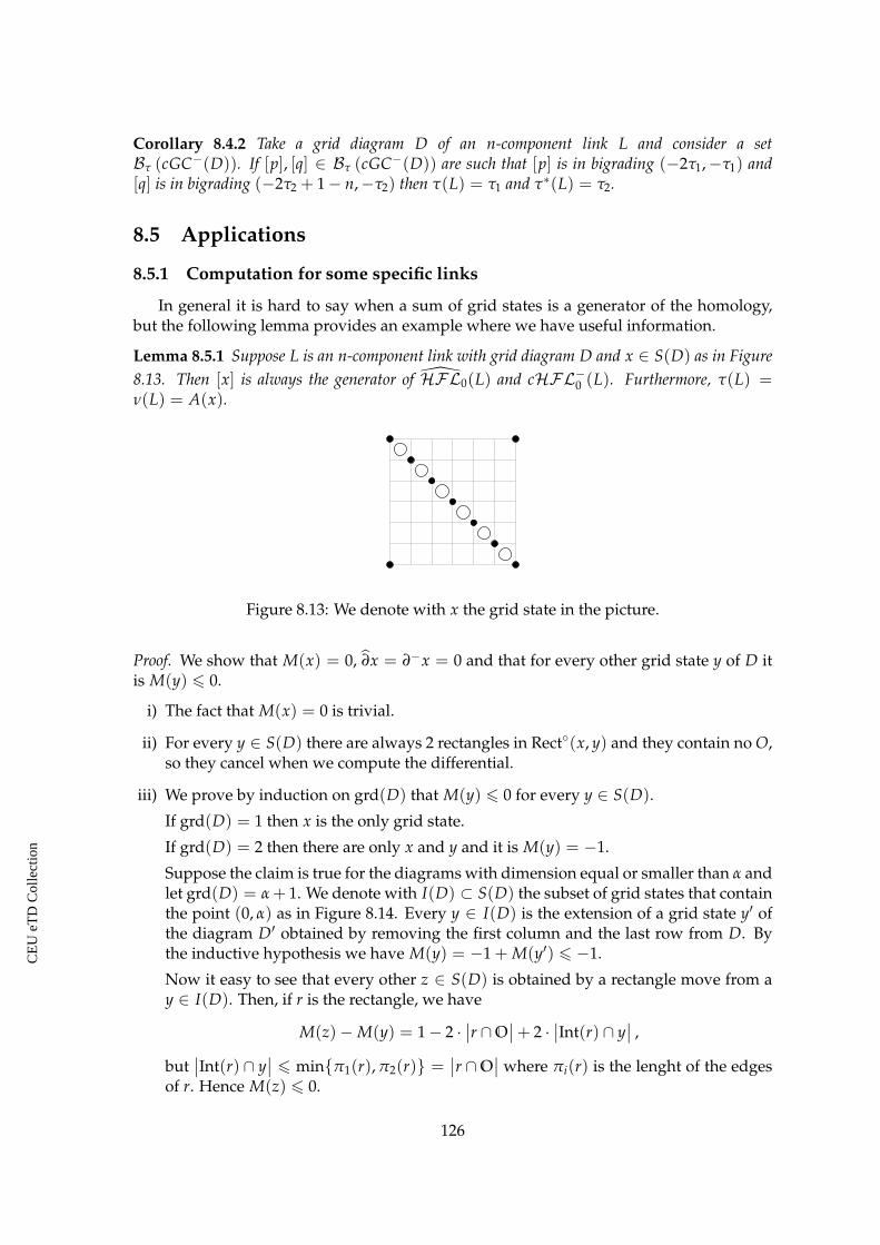
Corollary 8.4.2 Take a grid diagram D of an n-component link L and consider a setBτ (cGC−(D)). If [p], [q] ∈ Bτ (cGC−(D)) are such that [p] is in bigrading (−2τ1,−τ1) and[q] is in bigrading (−2τ2 + 1− n,−τ2) then τ(L) = τ1 and τ∗(L) = τ2.
8.5 Applications
8.5.1 Computation for some specific links
In general it is hard to say when a sum of grid states is a generator of the homology,but the following lemma provides an example where we have useful information.
Lemma 8.5.1 Suppose L is an n-component link with grid diagram D and x ∈ S(D) as in Figure8.13. Then [x] is always the generator of HFL0(L) and cHFL−0 (L). Furthermore, τ(L) =ν(L) = A(x).
Figure 8.13: We denote with x the grid state in the picture.
Proof. We show that M(x) = 0, ∂x = ∂−x = 0 and that for every other grid state y of D itis M(y) 6 0.
i) The fact that M(x) = 0 is trivial.
ii) For every y ∈ S(D) there are always 2 rectangles in Rect◦(x, y) and they contain no O,so they cancel when we compute the differential.
iii) We prove by induction on grd(D) that M(y) 6 0 for every y ∈ S(D).
If grd(D) = 1 then x is the only grid state.
If grd(D) = 2 then there are only x and y and it is M(y) = −1.
Suppose the claim is true for the diagrams with dimension equal or smaller than α andlet grd(D) = α + 1. We denote with I(D) ⊂ S(D) the subset of grid states that containthe point (0, α) as in Figure 8.14. Every y ∈ I(D) is the extension of a grid state y′ ofthe diagram D′ obtained by removing the first column and the last row from D. Bythe inductive hypothesis we have M(y) = −1 + M(y′) 6 −1.
Now it easy to see that every other z ∈ S(D) is obtained by a rectangle move from ay ∈ I(D). Then, if r is the rectangle, we have
M(z)−M(y) = 1− 2 ·∣∣r ∩O
∣∣+ 2 ·∣∣Int(r) ∩ y
∣∣ ,
but∣∣Int(r) ∩ y
∣∣ 6 min{π1(r), π2(r)} =∣∣r ∩O
∣∣ where πi(r) is the lenght of the edgesof r. Hence M(z) 6 0.
126
CE
UeT
DC
olle
ctio
n

(0, α)
Figure 8.14: The state y ∈ I(D) is marked with the black circles.
In Lemma 8.5.1 we used that the grid diagram D has all the O-markings aligned on adiagonal. It is easy to see that if a link admits such a diagram then it is positive. On theother hand, it seems difficult for the converse to be true.
8.5.2 Torus links
We compute the τ-invariant of every torus link. Consider the grid diagram Dq,p in Fig-ure 8.15, representing the torus link Tq,p with q 6 p and all the components oriented in thesame direction. From Lemma 8.5.1 we know that [x] is the only generator of HFL0(Tq,p).
XX
X
XX
XX
q
p
Figure 8.15: x is the grid state in the picture.
If we denote with n the number of components of Tq,p then a simple computation gives
A(x) =12(
M(x)−MX(x)− grd(Dq,p) + n)=
12(−MX(x)− p− q + n) =
=12
[2
q−1
∑i=1
i + q(p− q + 1)− p− q + n
]=
12[q(q− 1) + q(p− q + 1)− p− q + n] =
=12(pq− p− q + n) =
(p− 1)(q− 1)− 1 + n2
.
Now we use Lemma 8.5.1 again and obtain that
τ(Tq,p) =(p− 1)(q− 1)− 1 + n
2.
127
CE
UeT
DC
olle
ctio
n

Using the lower bound of Equation (8.9) gives a different way to compute the slice genusof a torus link with respect to what we did in [8]:
g4(Tq,p) >(p− 1)(q− 1)
2− 1− n
2+ 1− n =
(p− 1)(q− 1) + 1− n2
.
Since the Seifert algorithm applied to the standard diagram of Tq,p gives the opposite in-equality, we conclude that
g4(Tq,p) =(p− 1)(q− 1) + 1− n
2for any q 6 p .
8.5.3 Applications to Legendrian invariants
We equip S3 with its unique tight contact structure ξst, whose definition can be foundin Section 3.4. We remark that, if D = D1 ∪ ... ∪ Dn is a front projection of the Legendrianlink L in the standard contact 3-sphere, the Thurston-Bennequin and rotation number ofL are given by
tb(L) =n
∑i=1
tbi(L) and rot(L) =n
∑i=1
roti(L)
wheretbi(L) = wr(Di) + lk (Di,D \Di)−
12|cusps in Di|
and
roti(L) =12
(|down-ward cusps in Di| − |up-ward cusps in Di|
).
More information can be found in Section 3.2.
Proposition 8.5.2 Consider a Legendrian n-component link L of link type L in S3 equipped withthe standard contact structure. Then the following inequality holds:
tb(L) + | rot(L)| 6 2τ(L)− n . (8.13)
Proof. If L is a Legendrian link then, from [67], we know that L can be represented by agrid diagram D of the link L∗ (the mirror of L). This diagram D is such that
tbi(L)− roti(L) + 12
= Ai(x+)tbi(L) + roti(L) + 1
2= Ai(x−)
tb(L)− rot(L) + 1 = M(x+) tb(L) + rot(L) + 1 = M(x−) ,
where x± are the grid states in D obtained by taking a point in the northeast (southwest forx−) corner of every square decorated with an X ∈ X. Moreover, Ai is defined as follows:
Ai(x) = J(
x− 12(X + O), (Xi −Oi)
)− grd(D)i − 1
2for any x ∈ S(D)
with Oi ⊂ O and Xi ⊂ X the markings on the i-th component of L∗ and grd(D)i thenumber of elements in Oi.
In [67] is proved that x± represent non-torsion elements in the homology groupcHFL−(L∗); in fact these classes are the Legendrian grid invariants λ±(L). Since A(x) =
128
CE
UeT
DC
olle
ctio
n

n
∑i=1
Ai(x) for every grid state x, we have that M (x±) = 2A (x±) + 1− n. Therefore, Corol-
lary 8.4.2 implies that A (x±) 6 −τ∗(L∗). Combining the latter claim with Corollary 8.2.6,that gives τ∗(L∗) = −τ(L), we have
tb(L)∓ rot(L) + n2
= A(x±) 6 τ(L)
that is precisely Equation (8.13).
From Equation (8.13), together with Equation (8.9), we obtain the following lowerbound for the slice genus:
tb(L) + | rot(L)| 6 2g4(L) + n− 2 6 2u(L)− n , (8.14)
where u(L) is the unlinking number of L; see [55].This bound is sharp for positive torus links, but here we show that there are other links
for which this happens.In Figure 8.16 we have a front projection D of a Legendrian two component link L.
The link type of L is the link L9n19. A simple computation gives tb(L) = 6 and rot(L) = 0,
therefore Equation (8.14) says that g4(L9n19) > 3. Since it is easy to see that the link repre-
sented by D can be unlinked by changing the four crossings highlighted in the picture, wehave g4(L9n
19) 6 u(L9n19)− 1 6 3 and then we conclude that g4(L9n
19) = 3.
Figure 8.16: A diagram of the link L9n19.
From Equation (8.13) we also have the following upper bound for the maximalThurston-Bennequin number.
Proposition 8.5.3 For every n-component link L we have
TB(L) 6 2τ(L)− n .
Furthermore, if L is a quasi-alternating link then we have that
TB(L) 6 −1− σ(L) .
Although this bound is much less powerful than the Kauffmann or the HOMFLY poly-nomial, we can still get some interesting conclusions.
Consider a Legendrian link L such that each component Li is algebraically unlinked.Then tbi(L) = tb(Li) and so tb(L) is precisely the sum of the Thurston-Bennequin num-bers of its components. For example this happens for the Borromean link B, whose com-ponents Bi are three (algebraically unlinked) unknots. It was shown in [61] that there is no
129
CE
UeT
DC
olle
ctio
n

−2k +2k
Figure 8.17: A diagram of Lk. For k = 0 we have the link L9a40.
Legendrian representation of B, where the Thurston-Bennequin number of each compo-nent is -1; in fact we have TB(B) = −4, while TB(©) = −1. In particular, this means thatthe difference between TB(B) and the sum of TB(Bi) is -1.
We prove Proposition 8.5.4, where we give a family of 2-components links Lk such thatthe components of Lk are two unknots with lk(Lk
1, Lk2) = 0 and the difference between
TB(Lk) and the sum of TB(Lki ) is actually arbitrarily small, improving the latter result for
B. The links Lk are shown in Figure 8.17.
Proposition 8.5.4 The links Lk in Figure 8.17 are a family of two component links, whose compo-nents Lk
i are unknots with linking number zero, such that TB(Lk) is arbitrarily small.
Proof. Since for every k > 0 the link Lk is non-split alternating, we can easily computethe signature that is equal to 3 + 2k. Now we apply Proposition 8.5.3 and we obtain thatTB(Lk) 6 −4− 2k.
As a final obervation, we note that the same argument used by Baldwin, Vela-Vick andVértesi in [3] gives that the invariant L(L) defined in Chapter 6, for Legendrian links inthe standard contact 3-sphere, coincides with the grid invariant λ+(L) of [67].
130
CE
UeT
DC
olle
ctio
n

Chapter 9
Quasi-positive links in the 3-sphere
9.1 Maximal self-linking number and the slice genus
A quasi-positive link is any link which can be realized as the closure of a d-braid of theform
b
∏i=1
wiσji w−1i ,
where σj for j = 1, ..., d − 1 are the generators of the d-braids group that we defined inSubsection 3.4.2. Thus quasi-positive links are closures of braids consisting of arbitraryconjugates of positive generators.
It is worth noting that quasi-positive links are equivalent to another, more geometricclass of links: the transverse C-links. These links arise as the transverse intersection of the3-sphere S3 ⊂ C2, with a complex curve. Transverse C-links include links of isolated curvesingularities, but are in fact a much larger class. The fact that quasi-positive links can berealized as transverse C-links is due to Rudolph [80], while the fact that every transverseC-link is quasi-positive is due to Boileau and Orekov [6].
Given a quasi-positive braid B = (w1σj1 w−11 ) · ... · (wbσjb w−1
b ), we can associate to B asurface ΣB as follows. Let us consider the braid B′, obtained by removing the σji ’s from
B
ΣB
r1 r2
B′
Figure 9.1: The disk ΣB constructed from the quasi-positive braid B, representing the un-knot. The segments r1 and r2 are ribbon intersections.
131
CE
UeT
DC
olle
ctio
n

the presentation of B. Then B′ is the boundary of d disks with some ribbon interesctionsbetween themselves. If we push these disks in the 4-ball D4 then the intersections disap-pear and we obtain a surface which is properly embedded in D4. At this point, we add bpositive bands in correspondence of the σji ’s; the result is an oriented and compact surfacethat is not embedded in S3, but it is properly embedded in D4, whose boundary is clearlythe closure of the braid B. See Figure 9.1 for an example.
A connected transverse C-link is a link which is the closure of a quasi-positive braid Bsuch that ΣB is connected. Then we have the following proposition.
Proposition 9.1.1 Every connected transverse C-link is non-split quasi-positive.
Proof. Suppose that B is a quasi-positive braid, presented as before, such that ΣB is con-nected and its closure L is a split link. Then we can write L = L1 t L2 and Li is the closureof the subbraid Bi for i = 1, 2.
Since lk(L1, L2) = 0, we have that the arcs corresponding to the σji ’s both belong toB1 or B2. Therefore, there is no positive band connecting a disk, which appears in theconstruction of ΣB1 , with the ones in ΣB2 . This implies that ΣBi is a connected componentof ΣB for i = 1, 2 and this is a contradiction.
Later, in Corollary 9.2.4 we show that this inclusion is strict.The Thurston-Bennequin inequality stated in Section 3.6 can be improved using the
invariant τ(L), defined from the filtered link Floer homology group HFL(L) in Chapter8. More specifically, in Subsection 8.5.3 we prove Equation (8.13):
tb(L) + | rot(L)| 6 2τ(L)− n ,
where L is an n-component Legendrian link in the tight 3-sphere. From this result weobtain the following corollary.
Corollary 9.1.2 Suppose that L is an n-component Legendrian link in (S3, ξst) with smooth linktype L. Then we have that
sl(T ±L ) 6 tb(L) + | rot(L)| 6 2τ(L)− n 6 −χ(Σ) , (9.1)
where Σ is an oriented, compact surface, properly embedded in D4, such that ∂Σ = L.
Proof. The first two inequalities follow from Proposition 3.3.2 and Equation (8.13). The lastone is a consequence of Proposition 8.3.8.
It is interesting to observe that Equation (9.1) is a version of the adjunction inequality,see [52, 56].
We recall that, from the Thurston-Bennequin inequality, a transverse link in (S3, ξst)has bounded self-linking number. This means that we can denote the maximal self-linkingnumber of a link L with SL(L).
Theorem 9.1.3 Suppose that L is an n-component quasi-positive link in S3. Then we have that
SL(L) = b− d and τ(L) =b− d + n
2,
where L is the closure of a quasi-positive d-braid B = (w1σj1 w−11 ) · ... · (wbσjb w−1
b ).
132
CE
UeT
DC
olle
ctio
n
Proof. As we saw in Subsection 3.4.2, the braid B determines a transverse link T in (S3, ξst)and
sl(T ) = wr(B)− d = b− d .
Then from Theorem 6.6.5 and Equation (9.1) we have that
sl(T ) 6 SL(L) 6 2τ(L)− n 6 −χ(ΣB) = b− d
and these inequalities are all equalities.
When we consider connected surfaces, the inequality in Equation (9.1) becomes
sl(T ) 6 2τ(L)− n 6 2g4(L) + n− 2 , (9.2)
for every n-component transverse link T in (S3, ξst), with link type L, and where we recallthat g4(L) is the minimal genus of a compact, oriented surface Σ properly embedded in D4
and such that ∂Σ = T , see Section 1.3. Then we have the following proposition.
Proposition 9.1.4 Suppose that L is an n-component link, embedded in S3, which is a connectedtransverse C-link. Then we have that τ(L) = g4(L) + n− 1.
Proof. The claim follows from the same argument in the proof of Theorem 9.1.3 and Equa-tion (9.2).
An implication of this proposition is the additivity of the slice genus under connectedsums.
Corollary 9.1.5 The slice genus g4 is additive under connected sums if we restrict to the family ofconnected transverse C-links.
Proof. If L1 and L2 are two connected transverse C-links then it is easy to see that everyconnected sum L = L1# L2 has the same property. In fact, take two quasi-positive braids,representing L1 and L2; then L is obtained by putting the second below the first one andadding a positive band between the components that we want to sum, say the i-th and thej-th ones with i < j. This move can be seen as the composition of B with wσj−1w−1 forsome w and then the resulting braid is still quasi-positive.
Therefore, Proposition 9.1.4 gives that τ(Li) = g4(Li) + ni − 1, where ni are the num-ber of components of Li for i = 1, 2. Moreover, what we said before also implies thatτ(L) = g4(L) + (n1 + n2 − 1) − 1. At this point, we use that the invariant τ is additiveunder connected sums of links, see Equation (8.7) in Subsection 8.2.3, and then the proofis complete.
In Theorem 9.1.3 we showed a way to compute the τ-invariant for quasi-positive links,using braids. It is known that a similar formula holds for the Rasmussen link invariant s,see [76, 83]. Then we can prove Proposition 9.1.6, which says that the two invariants arerelated to each other in this case.
Proposition 9.1.6 Take an n-component quasi-positive link L in the 3-sphere. Then the invariantτ(L) from link Floer homology and the invariant s(L) from Khovanov homology satisfy the relation
s(L) = 2τ(L) + 1− n .
Proof. The invariant s(L) can be computed from a quasi-positive braid B, presented asusual in this section, in the following way:
s(L) = b− d + 1 .
This is proved in [76, 83]. Then the statement follows immediately from Theorem 9.1.3.
133
CE
UeT
DC
olle
ctio
n

9.2 Strongly quasi-positive links
We apply the results obtained in Chapter 8 and in the previous subsection to recomputethe invariant tau for strongly quasi-positive links in S3. A link L ↪→ S3 is strongly quasi-positive if it is the boundary of a quasi-positive surface F. Such surfaces are constructed
1
2
3
4
Figure 9.2: The quasi-positive surface determined by d = 4 and~b = (σ13, σ24, σ13, σ24).
in the following way: take d disjoint parallel, embedded disks, all of them oriented in thesame way, and attach b negative bands on them, each one between a pair of distinct disks.This procedure is shown in Figure 9.2. The negative bands cannot be knotted with eachother; this means that, up to isotopy, F only depends on the number d and the orderedb-tuple~b = (σi1 j1 , ..., σib jb), where σij denotes that a negative band is put between the i-thand the j-th disk with i < j.
Denote with σ1, ..., σd−1 the generators of the d-braids group. Then it is easy to see thatthe boundary of the quasi-positive surface (1, σij) is isotopic to the closure of the d-braidgiven by {
(σi · · · σj−2)σj−1(σi · · · σj−2)−1 if j > i + 2
σi if j = i + 1;
see [44] for more details. This immediately implies that strongly quasi-positive links arequasi-positive.
Suppose S3 is equipped with its unique tight contact structure ξst and L ↪→ (S3, ξst)is an n-component transverse link with smooth link type L. Then we have the followingcorollary.
Corollary 9.2.1 Suppose that T is an n-component transverse link in (S3, ξst) with smooth linktype L. Then we have that
sl(T ) 6 2τ(L)− n 6 ‖L‖T − o(L) ,
where o(L) is the number of disjoint unknots in L.
Proof. The first inequality follows immediately from Equation (9.2). For the second one weapply Theorem 2.1.2; in fact, it is known, see [67], that the group HFL∗,∗(L) is non-zero inbigrading (0, τ(L)).
134
CE
UeT
DC
olle
ctio
n

We recall that ‖L‖T is the Thurston norm of L, see Chapter 2. Then we can now provethe following theorem.
Theorem 9.2.2 Consider a strongly quasi-positive link L with n components in S3. Then theThurston-Bennequin inequality is sharp for L, in the sense that there exists a transverse represen-tative T of L such that
sl(T ) = 2τ(L)− n = ‖L‖T − o(L) = −χ(F) ,
where o(L) is the number of disjoint unknots in L and F is a quasi-positive surface for L. In
i
j
i
j
Figure 9.3: Transverse realization of L1.
particular
τ(L) =‖L‖T − o(L) + n
2=
b− d + n2
,
where F consists of d disks and b negative bands.
Proof. From Lemma 2.2.5 and Corollary 9.2.1 it is enough to show that, given a quasi-positive surface F whose boundary is L, we can find a transverse link T , with smooth linktype L, such that sl(T ) = b− d.
Let us start with the d parallel disks in F and see what happens when we attach thefirst negative band. The surface we obtain is the quasi-positive surface determined by dand~b = (σij), where i < j correspond to the disks on which we glue the negative band,and we call L1 its boundary.
At this point, we choose a transverse representative of L1 as shown in Figure 9.3. ThenT is defined by iterating this procedure with all the b bands and, since we computed itsself-linking number in the previous section, we obtain that
sl(T ) = b− d .
This proves the claim.
Since we remarked in the proof of Corollary 9.2.1 that HFL0,τ(L)(L) 6= {0}, Theorems2.1.2 and 9.2.2 tell us that for strongly quasi-positive links
τ(L) = max{
s ∈ Z | HFL∗,s(L) 6= {0}}
.
Furthermore, applying Lemma 2.2.5 to Theorem 9.2.2, we can say more when the link Lalso bounds a connected quasi-positive surface, that we call quasi-positive Seifert surface forL.
Corollary 9.2.3 If L is a link as in Theorem 9.2.2, which also admits a quasi-positive Seifert surfaceF′, then we have that
τ(L) = g3(L) + n− 1 = g(F′) + n− 1 ,
where g3(L) is the Seifert genus of L.
135
CE
UeT
DC
olle
ctio
n

This corollary implies that all the quasi-positive Seifert surfaces of a given link havethe same genus. Moreover, we observe that not every strongly quasi-positive link admitsa quasi-positive Seifert surface. In fact, the 4-component link L in Figure 9.2 is such thatτ(L) = 2 from Theorem 9.2.2, but L has Seifert genus zero: to see this it is enough to add atube between disks 1 and 2 in Figure 9.2. Then we have that
2 = τ(L) 6= g3(L) + n− 1 = 3
and so this would contradict Corollary 9.2.3. This argument also implies the followingcorollary.
Corollary 9.2.4 The link L in Figure 9.2 is non-split quasi-positive, but it is not a connectedC-transverse link.
Proof. By construction L is non-split strongly quasi-positive and then it is quasi-positive. Ifwe suppose that L is a connected transverse C-link then we can use Proposition 9.1.4 andwe obtain that
g4(L) = τ(L) + 1− n = −1
which is clearly impossible.
9.3 The case of positive links
We recall that, from [81], positive links are always strongly quasi-positive. Moreover,if a link is positive non-split then it also admits a quasi-positive Seifert surface. This meansthat the results in Section 9.2 also hold in this case. Moreover, we state a proposition from[49], which tells us that the maximal Thurston-Bennequin number TB of a positive link canbe determined easily.
Proposition 9.3.1 (Kálmán) Suppose that L is an n-component link in S3 with a positive diagramD. Then we have that
TB(L) = c(D)− k(D) ,
where c(D) and k(D) are the numbers of crossings in D and of circles in the oriented resolution ofD.
We want to prove the following corollary.
Corollary 9.3.2 Suppose that L is a link as in Proposition 9.3.1 with split components L1, ..., Lr.Then we have that
TB(L) = 2τ(L)− n = 2g3(L) + n− 2r .
When a link has a diagram D which is positive, the oriented resolution defined in Sub-section 1.2.2 happens to possess some peculiar properties. Let us start with the followinglemma.
Lemma 9.3.3 Suppose that D is a positive diagram for a link L and consider D′ ⊂ D a subdiagram,which represents a split component L′ of L.
Then the surface F′, obtained from the oriented resolution of D′, is contained as subset in F, theone obtained in the same way from D.
136
CE
UeT
DC
olle
ctio
n

Proof. The surface F′ is completely determined by K′, the collection of circles in the ori-ented resolution of D′, and the crossings in D′. Denote with K the circles in the orientedresolution of D. If C ∈ K′ then C ∈ K; this is because lk(L′, L \ L′) = 0, since L′ is a splitcomponent of L. Therefore, there is no crossing between D′ and D \ D′, because D is posi-tive, and then neither between K′ and K \K′. Moreover, the crossings in D′ also appear inD because D′ is a subdiagram of D.
It follows that F′ ⊂ F and F \ F′ is precisely the surface obtained from the orientedresolution of D \ D′. This appears clearly from Figure 1.7.
In order to prove Proposition 9.3.1 we need another lemma.
Lemma 9.3.4 Suppose that D is a positive diagram for a link L = L1 t ...t Lr, where {Li}ri=1 are
the split components of L.Then the surface F, obtained from the oriented resolution of D, can be isotoped into F1 t ...t Fr;
where each Fi is a Seifert surface for Li. Furthermore, Fi is obtained from the oriented resolution ofDi ⊂ D, the subdiagram representing Li, for every i = 1, ..., r.
Proof. Let us work on the case when L is non-split first. The surface F is compact andoriented, but now it is also connected; in fact, otherwise we could write D = D1 ∪ D2
where there is no crossing between D1 and D2. This implies that, if D ⊂ {z = 0} in R3, wecould push D2 up in the plane {z = 1} and then move it away from D1. This determinesan isotopy of S3 and then L would be split, which is a contradiction.
Now, for the general case, we observe that, from Lemma 9.3.3 and the non-split case wedid before, the surface F possesses as connected components the surfaces {Fi}r
i=1 each onebeing a Seifert surface for Li; moreover, the Fi’s are obtained from the oriented resolutionof the subdiagrams Di ⊂ D that represent Li for i = 1, ..., r.
We want to isotope F in a way that it becomes the disjoint union of F1, ..., Fr. To dothis we consider the planar subspaces D and {Di}r
i=1 of R2, associated to D and {Di}ri=1
respectively as in Subsection 1.2.2, and we call Fi an innermost component of F if only onecomponent of R2 \ Di intersects F. Hence, we reason in the same way as before and wepush Fi slightly up from the plane and move it away from F \ Fi. We repeat this procedurefor all the components of F and at the end the surface will be as we wanted.
We are now ready to prove Corollary 9.3.2.
Proof of Proposition 9.3.1 and Corollary 9.3.2. We suppose first that L is a non-split link. Thenfrom Corollaries 9.1.2 and 9.2.1 we know that each Legendrian representative of L satisfiesthe following inequality:
tb(L) 6 TB(L) 6 2τ(L)− n = 2g3(L) + n− 2 6 −χ(F) = c(D)− k(D) ; (9.3)
where F is the surface obtained from the oriented resolution of D, which is a Seifert surfacefor Lemma 9.3.4. The first equality follows from the fact that a non-split positive linkadmits a quasi-positive Seifert surface and Corollary 9.2.3.
We define the Legendrian link L in the following way. Let us consider the planarsubspace D of R2, associated to D, and the set K consisting of the circles in the orientedresolution. We isotope the circles in K, starting from the innermost ones, until they haveonly two vertical tangency points, one on the left and the other one on the right of thecircle. At this point, we isotope D in a way that the lines between the circles in K appear
137
CE
UeT
DC
olle
ctio
n

D
L
Figure 9.4: Legendrianization of an oriented resolution.
vertical in the plane, see Figure 9.4; this is done by moving the innermost ones first asbefore, more details can be found in [49].
Then we just change the vertical tangencies into cusps and the vertical lines into cross-ings; we obtain the front projection of a Legendrian link because D is positive and thenall the lines correspond to negative bands. An easy computation gives that tb(L) =c(D) − k(D) and rot(L) = 0, which means that all the inequalities in Equation (9.3) areequalities.
Suppose now that L = L1 t ... t Lr. Take the Legendrian links Li, representing Lifor i = 1, ..., r, defined following the same procedure as before and denote with L theLegendrian link L1 t ...t Lr. Then we have that
tb(L) =r
∑i=1
tb(Li) =r
∑i=1
c(Di)− k(Di) = c(D)− k(D) , (9.4)
where Di ⊂ D is the subdiagram representing Li. Here the final equality follows fromLemma 9.3.4. The Thurston-Bennequin inequality in Corollary 9.2.3 again gives
tb(L) 6 TB(L) 6 2τ(L)− n = ‖L‖T − o(L) 6r
∑i=1
(2g3(Li) + ni − 1) 6
6 −r
∑i=1
χ(Fi) = c(D)− k(D) ,(9.5)
where Fi are the Seifert surfaces obtained from the oriented resolution of Di for i = 1, ..., r,the number o(L) tells us how many disjoint unknots there are in L and ni is the numberof components of each Li. We also used Proposition 2.2.2. Clearly, Equation (9.4) says thatall the inequalities in Equation (9.5) are equalities and then the claim follows from the factthat
r
∑i=1
(2g3(Li) + ni − 1) = 2r
∑i=1
g3(Li) + n− r = 2g3(L) + n− r ,
where the final equality holds because the Seifert genus is additive under disjoint unions.
138
CE
UeT
DC
olle
ctio
n

The invariant τ(L) of a positive link can be determined from the oriented resolution ofa positive diagram D for L. In fact, Proposition 9.3.1 and its proof immediately imply thefollowing corollary.
Corollary 9.3.5 Suppose L is a positive n-component link in S3 with r split components. Then wehave that
τ(L) =r
∑i=1
g(Fi) + n− r =c(D)− k(D) + n
2,
where {Fi}ri=1 are the connected components of the surface obtained from the oriented resolution of
a positive diagram D for L, while c(D) and k(D) are as in Proposition 9.3.1.
In particular, all the surfaces obtained from the oriented resolution of a positive dia-gram for a given link have the same genus. Furthermore, Corollary 9.3.5 also gives that apositive link admits a quasi-positive Seifert surface if and only if it is non-split.
139
CE
UeT
DC
olle
ctio
n
CE
UeT
DC
olle
ctio
n

Bibliography
[1] M. F. Atiyah and I. G. Macdonald, Introduction to commutative algebra, Addison-WesleyPublishing Co., Reading, Mass.-London-Don Mills, Ont. 1969, pp. ix+128.
[2] K. Baker and J. Etnyre, Rational linking and contact geometry, Progr. Math., 296,Birkhäuser/Springer, New York, 2012.
[3] J. Baldwin, D. S. Vela-Vick and V. Vértesi, On the equivalence of Legendrian and transverseinvariants in knot Floer homology, Geom. Topol., 17 (2013), no. 2, pp. 925-974.
[4] D. Bennequin, Entrelacements et équations de Pfaff, Astérisque, 107-108 (1983), pp. 87-161.
[5] J. Birman, Braids, Links, and Mapping Class Groups, Annals of Math. Studies 82, Prince-ton University Press, Princeton 1975.
[6] M. Boileau and S. Orevkov, Quasipositivite dune courbe analytique dans une boule pseudo-convexe, C. R. Acad. Sci. Paris., 332 2001, pp. 825-830.
[7] D. Calegari, Foliations and the geometry of 3-manifolds, Oxford Mathematical Mono-graphs, Oxford University Press, Oxford, 2007.
[8] A. Cavallo, On the slice genus and some concordance invariants of links, J. Knot TheoryRamifications, 24 (2015), no. 4, 1550021.
[9] A. Cavallo, The concordance invariant tau in link grid homology, to appear on Alg. Geom.Topol., arXiv:1512.08778.
[10] A. Cavallo, An invariant of Legendrian and transverse links from open book decompositionsof contact 3-manifolds, arXiv:1711.09508.
[11] A. Cavallo, On loose Legendrian knots in rational homology spheres, Topology Appl., 235(2018), pp. 339-345.
[12] A. Cavallo, On Bennequin type inequalities for links in tight contact 3-manifolds,arXiv:1801.00614.
[13] V. Colin, Chirurgies d’indice un et isotopies de sphères dans les variétés de contact tendues,C. R. Acad. Sci. Paris Sér. I Math., 324 (1997), pp. 659-663.
[14] O. Dasbach and B. Mangum, On McMullen’s and other inequalities for the Thurston normof link complements, Algebr. Geom. Topol., 1 (2001), pp. 321-347.
[15] F. Ding and H. Geiges, A Legendrian surgery presentation of contact 3-manifolds, Math.Proc. Cambridge Philos. Soc., 136 (2004), no. 3, pp. 583-598.
141
CE
UeT
DC
olle
ctio
n

[16] F. Ding and H. Geiges, A unique decomposition theorem for tight contact 3-manifolds, En-seign. Math. (2), 53 (2007), no. 3-4, pp. 333-345.
[17] K. Dymara, Legendrian knots in overtwisted contact structures on S3, Ann. Global Anal.Geom., 19 (2001), no. 3, pp. 293-305.
[18] Y. Eliashberg, Classification of overtwisted contact structures on 3-manifolds, Invent.Math., 98 (1989), no. 3, pp. 623-637.
[19] Y. Eliashberg, Topological characterization of Stein manifolds of dimension > 2, Int. J. ofMath., 1 (1990), pp. 29-46.
[20] Y. Eliashberg, On symplectic manifolds with some contact properties, J. Diff. Geom., 33(1991), pp. 233-238.
[21] Y. Eliashberg, Contact 3-manifolds twenty years since J. Martinet’s work, Ann. Inst.Fourier (Grenoble), 42 (1992), no. 1-2, pp. 165-192.
[22] Y. Eliashberg, Classification of contact structures on R3, Internat. Math. Res. Notices.,(1993), no. 3, pp. 87-91.
[23] Y. Eliashberg, Legendrian and transversal knots in tight contact 3-manifolds, Topologicalmethods in modern mathematics, pp. 171-193, Publish or Perish, Houston, TX, 1993.
[24] Y. Eliashberg and M. Fraser, Classification of topologically trivial Legendrian knots, CRMProc. Lecture Notes, 15, Amer. Math. Soc., Providence, RI, 1998.
[25] Y. Eliashberg and M. Gromov, Convex symplectic manifolds, Proc. Sympos. Pure Math.,52, Part 2, Amer. Math. Soc., Providence, RI, 1991.
[26] J. Etnyre, Legendrian and transversal knots. Handbook of knot theory, Elsevier B. V., Ams-terdam, 2005, pp. 105-185.
[27] J. Etnyre, Lectures on open book decompositions and contact structures, Clay Math., Proc.(5), Amer. Math. Soc., Providence, RI, 2006, pp. 103-141.
[28] J. Etnyre, On contact surgery, Proc. Amer. Math. Soc., 136 (2008), no. 9, pp. 3355-3362.
[29] J. Etnyre, On knots in overtwisted contact structures, Quantum Topol., 4 (2013), no. 3, pp.229-264.
[30] J. Etnyre and K. Honda, Knots and contact geometry I: torus knots and the figure eight,Journal of Sympl. Geom., 1 (2001), no. 1, pp. 63-120.
[31] J. Etnyre and K. Honda, On connected sums and Legendrian knots, Adv. Math., 179(2003), no. 1, pp. 59-74.
[32] A. Floer, A relative Morse index for the symplectic action, Comm. Pure Appl. Math., 41(1988), no. 4, pp. 393-407.
[33] A. Floer, The unregularized gradient flow of the symplectic action, Comm. Pure Appl.Math., 41 1988,no. 6, pp. 775-813.
[34] R. Fox and J. Milnor, Singularities of 2-spheres in 4-space and cobordism of knots, Osaka J.Math., 3 (1966), pp. 257-267.
142
CE
UeT
DC
olle
ctio
n

[35] H. Geiges, Contact geometry, Handbook of differential geometry. Vol. II, pp. 315-382,Elsevier/North-Holland, Amsterdam, 2006.
[36] P. Ghiggini, Strongly fillable contact 3-manifolds without Stein fillings, Geom. Topol., 9(2005), pp. 1677-1687.
[37] E. Giroux, Convexité en topologie de contact, Comment. Math. Helv., 66 (1991), no. 4, pp.637-677.
[38] E. Giroux, Structures de contact en dimension trois et bifurcations des feuilletages de surfaces,Invent. Math., 141 (2000), no. 3, pp. 615-689.
[39] E. Giroux, Géométrie de contact: de la dimension trois vers les dimensions supérieures, Pro-ceedings of the International Congress of Mathematicians, Vol. II, Higher Ed. Press,Beijing, 2002, pp. 405-414.
[40] R. Gompf, Handlebody construction of Stein surfaces, Ann. of Math. (2), 148 (1998), no. 2,pp. 619-693.
[41] R. Gompf and A. Stipsicz, 4-manifolds and Kirby calculus, Graduate Studies in Mathe-matics, 20. American Mathematical Society, Providence, RI, 1999, pp. xvi+558.
[42] M. Gromov, Pseudoholomorphic curves in symplectic manifolds, Invent. Math., 82 (1985),no. 2, pp. 307-347.
[43] A. Hatcher, Algebraic topology, Cambridge University Press, Cambridge, 2002.
[44] M. Hedden, Notions of positivity and the Ozsváth-Szabó concordance invariant, J. KnotTheory Ramifications, 19 (2010), no. 5, pp. 617-629.
[45] J. Hom and Z. Wu, Four-ball genus bounds and a refinement of the Ozsváth-Szabó τ-invariant, J. Symplectic Geom., 14 (2016), no. 1, pp. 305-323.
[46] K. Honda, On the classification of tight contact structures I, Geom. Topol., 4 (2000), pp.309-368.
[47] K. Honda, W. Kazez and G. Matic, On the contact class in Heegaard Floer homology, J.Differential Geom., 83 (2009), no. 2, pp. 289-311.
[48] H. Hopf, Über die Abbildungen der dreidimensionalen Sphäre auf die Kugelfläche, Math.Ann., 104 (1931), pp. 637-665.
[49] T. Kálmán, Maximal Thurston-Bennequin number of +adequate links, Proc. Amer. Math.Soc., 136 (2008), no. 8, pp. 2969-2977.
[50] Y. Kanda, The classification of tight contact structures on the 3-torus, Comm. in Anal. andGeom., 5 (1997), pp. 413-438.
[51] A. Kawauchi, T. Shibuya and S. Suzuki, Descriptions on surfaces in four-space. I. Normalforms, Math. Sem. Notes Kobe Univ., 10 (1982), no. 1, pp. 75-125.
[52] P. Kronheimer and T. Mrowka, The genus of embedded surfaces in the projective plane,Math. Research Letters, 1 (1994), pp. 797-808.
143
CE
UeT
DC
olle
ctio
n

[53] J. Levine, Invariants of knot cobordism, Invent. Math., 8 (1969), pp. 98-110.
[54] J. Levine, Knot cobordism groups in codimension two, Comment. Math. Helv., 44 (1969),pp. 229-244.
[55] W. B. R. Lickorish, An introduction to knot theory, Graduate Texts in Mathematics, 175.Springer-Verlag, New York, 1997.
[56] P. Lisca and G. Matic, Stein 4-manifolds with boundary and contact structures, TopologyAppl., 88 (1998), no. 1-2, pp. 55-66.
[57] P. Lisca, P. Ozsváth, A. Stipsicz and Z. Szabó, Heegaard Floer invariants of Legendrianknots in contact three-manifolds, J. Eur. Math. Soc., 11 (2009), no. 6, pp. 1307-1363.
[58] C. Manolescu, P. Ozsváth, Z. Szabó and D. Thurston, On combinatorial link Floer homol-ogy, Geom. Topol., 11 (2007), pp. 2339-2412.
[59] J. Milnor, Lectures on the h-cobordism theorem, Princeton University Press, Princeton,NJ, 1965.
[60] J. Milnor and J. Stasheff, Characteristic classes, Annals of Mathematics Studies, No. 76.Princeton University Press, Princeton, NJ; University of Tokyo Press, Tokyo, 1974, pp.vii+331.
[61] K. Mohnke, Legendrian links of topological unknots, AMS, volume 279 of ContemporaryMathematics, 2001, pp. 209-211.
[62] Y. Ni, Link Floer homology detects the Thurston norm, Geom. Topol., 13 (2009), no. 5, pp.2991-3019.
[63] H. Ohta and K. Ono, Simple singularities and topology of symplectically filling 4-manifold,Comment. Math. Helv., 74 (1999), pp. 575-590.
[64] S. Orevkov and V. Shevchishin, Markov Theorem for Transverse Links, J. Knot TheoryRamifications, 12 (2003), no. 7, pp. 905-913.
[65] B. Ozbagci and A. Stipsicz, Surgery on contact 3-manifolds and Stein surfaces, BolyaiSociety Mathematical Studies, 13. Springer-Verlag, Berlin; János Bolyai MathematicalSociety, Budapest, 2004. pp. 281.
[66] P. Ozsváth and A. Stipsicz, Contact surgeries and the transverse invariant in knot Floerhomology, J. Inst. Math. Jussieu, 9 (2010), no. 3, pp. 601-632.
[67] P. Ozsváth, A. Stipsicz and Z. Szabó, Grid homology for knots and links, AMS, volume208 of Mathematical Surveys and Monographs, 2015.
[68] P. Ozsváth and Z. Szabó, Holomorphic disks and topological invariants of closed three-manifolds, Ann. of Math. (2), 159 (2004), no. 3, pp. 1159-1245.
[69] P. Ozsváth and Z. Szabó, Holomorphic disks and knot invariants, Adv. Math., 186 (2004),no. 1, pp. 58-116.
[70] P. Ozsváth and Z. Szabó, Heegaard Floer homology and contact structures, Duke Math. J.,129 (2005), no. 1, pp. 39-61.
144
CE
UeT
DC
olle
ctio
n

[71] P. Ozsváth and Z. Szabó, On the Heegaard Floer homology of branched double-covers, Adv.Math., 194 (2005), no. 1, pp. 1-33.
[72] P. Ozsváth and Z. Szabó, Holomorphic disks, link invariants and the multi-variable Alexan-der polynomial, Algebr. Geom. Topol., 8 (2008), no. 2, pp. 615-692.
[73] P. Ozsváth and Z. Szabó, Link Floer homology and the Thurston norm, J. Amer. Math.Soc., 21 (2008), no. 3, pp. 671-709.
[74] J. Pardon, The link concordance invariant from Lee homology, Algebr. Geom. Topol., 12(2012), no. 2, pp. 1081-1098.
[75] T. Perutz, Hamiltonian handleslides for Heegaard Floer homology, In Proceedings ofGökova Geometry-Topology Conference 2007, pp. 15-35. Gökova Geometry/TopologyConference (GGT), Gkova, 2008.
[76] O. Plamenevskaya, Transverse knots and Khovanov homology, Math. Res. Lett., 13 (2006),no. 4, pp. 571-586.
[77] O. Plamenevskaya, A combinatorial description of the Heegaard Floer contact invariant,Algebr. Geom. Topol., 7 (2007), pp. 1201-1209.
[78] J. Rasmussen, Floer homology and knot complements, Thesis (Ph.D.)-Harvard University,2003, pp. 126.
[79] D. Rolfsen, Knots and links, Mathematics Lecture Series, 7. Publish or Perish, Inc.,Houston, TX, 1990.
[80] L. Rudolph, Algebraic functions and closed braids, Topology, 22 1983, no. 2, pp. 191-202.
[81] L. Rudolph, Positive links are strongly quasipositive, Geom. Topol. Monogr., (2), Geom.Topol. Publ., Coventry, 1999.
[82] S. Sarkar, Grid diagrams and the Ozsváth-Szabó tau-invariant, Math. Res. Lett., 18 (2011),no. 6, pp. 1239-1257.
[83] A. Shumakovitch, Rasmussen invariant, slice-Bennequin inequality, and sliceness of knots,J. Knot Theory Ramifications, 16 (2007), no. 10, pp. 1403-1412.
[84] J. Singer, Three-dimensional manifolds and their Heegaard diagrams, Trans. Amer. Math.Soc., 35 (1933), no. 1, pp. 88-111.
[85] J. Swiatkowski. On the isotopy of Legendrian knots, Ann. Global Anal. Geom., 10 (1992),no. 3, pp. 195-207.
[86] W. Thurston, A norm for the homology of 3-manifolds, Mem. Amer. Math. Soc., 59 (1986),no. 339, pp. i-vi and 99-130.
[87] W. Thurston and H. Winkelnkemper, On the existence of contact forms, Proc. Amer.Math. Soc., 52 (1975), pp. 345-347.
[88] V. Turaev, Torsions of 3-manifolds, Geom. Topol. Monogr. 4, Geom. Topol. Publ., Coven-try, 2002.
145
CE
UeT
DC
olle
ctio
n

[89] T. Vogel, Non-loose unknots, overtwisted discs, and the contact mapping class group of S3,arXiv:1612.06557.
[90] F. Warner, Foundations of differentiable manifolds and Lie groups, Graduate Texts in Math-ematics, 94. Springer-Verlag, New York-Berlin, 1983. pp. ix+272.
[91] N. Wrinkle, The Markov theorem for transverse knots, Thesis (Ph.D.)-Columbia Univer-sity, 2002, pp. 51.
146
CE
UeT
DC
olle
ctio
n

Index
J-holomorphic strip, 57moduli space, 58
Spinc structure, 47relative, 49
τ-set, 124Rect, 107
Rect◦, 107
Abstract open book, 53–54associated to an adapted open book de-
composition, 55basepoint, 54monodromy, 53positive stabilization, 74strip position, 54
Alexander grading, 60, 106symmetry, 63
Alexander pair, 93Arc
dead, 51diagram, 12distinguished, 51separating, 51
Braid, 38–39Braids group, 39
Chain complex, 18associated to a grid diagram, 106–107,
113Alexander grading, 106Maslov grading, 106
associated to a Heegaard diagram, 58–62, 64
Alexander multi-grading, 60Maslov grading, 59
differential, 18filtered, 18
associated graded object, 18quasi-isomorphic, 19
filtered isomorphism, 20
homology, 18, 19maps, 19
Chain homotopyfiltered, 19
Chain homotopy equivalencefiltered, 19
Chain map, 19filtered, 19
associated mapping cone, 20Characteristic foliation, 42Classical invariants
Legendrian, 34, 38surgery presentation, 99–100transverse, 36, 39
Cobordism, 15birth, 118death, 119elementary, 16identity, 116merge, 117split, 116strong, 16torus, 117
Complexity, 25Component
of a link, 9split, 9
Compressibility term, 30Compressible surface, 28Concordance, 16Connected sum
contact, 40diagram, 15Legendrian, 40links, 10
Contact 3-manifold, 31contact cell decomposition, 51–53prime decomposition, 33Stein fillable, 33symplectically fillable, 33
147
CE
UeT
DC
olle
ctio
n
Contact framing, 31, 34Contact structure, 31
ξn, 33ξst, 37, 39overtwisted, 31
at infinity, 33tight, 31
at infinity, 33Contact surgery, 34Contact vector field, 32Contactomorphism, 31Convex surface, 32Cooriented 2-plane field, 31Crossing, 12
Darboux ball, 40Differential, 18
associated to a grid diagram, 107associated to a Heegaard diagram, 64associated to a multi-pointed Heegaard
diagram, 61–62mapping cone, 20
Disjoint union, 9, 29Legendrian, 42
Dividing set, 32
Elementary cobordism, 16Elementary tangle, 10
Legendrian, 40trivial, 10
Equivalenceof abstract open books, 54of filtered chain complexes, 19of links, 9
Filtered isomorphism, 20Filtration, 18
level, 18Front projection, 37Function T, 109
GenusSeifert, 9slice, 16
Graded object, 18Grid diagram, 105–106
grid state, 105stabilization with an unknot, 109–111
Grid homology, 107–108, 111, 123
invariance, 108–109, 111–112
Handlebody, 45Heegaard diagram
handleslide, 46Heegaard diagram, 45–46
admissible, 61basepoint, 46, 47, 50compatible Morse function, 46domain, 58handleslide, 48intersection point, 47Legendrian, 73–74multi-pointed, 47–48, 50
associated to an abstract open book,55
pointed, 46stabilization, 46, 48
Heegaard Floer homology, 64–66connected sum, 114disjoint union, 114invariance, 66–70
choice of the almost-complex struc-ture, 67–68
handleslide, 69isotopy, 68–69stabilization, 70
link, 57, 63mirror image, 113–114quasi-alternating links, 115unknot, 123unlink, 66, 111
Hopf invariant, 32Hopf link, 17
Invariant L, 80–81connected sum, 88disjoint union, 91gradings, 87–88invariance, 83–84
admissible arc slide, 82isotopy, 81–82positive stabilization, 82–83
stabilization, 91Invariant T, 81
gradings, 88invariance, 92
Invariant ν, 123
148
CE
UeT
DC
olle
ctio
n

Invariant τ, 111τ∗, 114connected sum, 114disjoint union, 114invariance, 120mirror image, 114positive links, 139quasi-alternating links, 115quasi-positive links, 133slice genus, 121–122strongly quasi-positive links, 135
Invariant c, 84invariance, 85–86
Isotopycontact, 31Legendrian, 34smooth, 9transverse, 36
Knot, 9compressible, 28concordance, 17Legendrian, 34loose, 95meridian, 10transverse, 36trivial, 9
Knot concordance group, 17
Lens space, 28Link, 9
cobordism, 15connected sum, 10diagram, 12Legendrian, 34linking number, 10loose, 95mirror image, 11oriented, 9positive, 136quasi-alternating, 115quasi-positive, 131slice, 16split, 9strongly quasi-positive, 134transverse, 36
Link L9a40, 130
Link L9n19, 129
Link type, 34simple, 103
Linking number, 10diagram, 14
Loose link, 95
Mapping cone, 20Markings
in a grid diagram, 105special O-marking, 105
Maslov grading, 59–60, 106Maslov index, 58Meridian, 10Mirror image, 11
diagram, 15Morse moves, 16
Non-loose, 95Non-split, 9Null-homologous link, 9
Open book decomposition, 50–51adapted to a Legendrian link, 51admissible arc slide, 77–78associated to a contact cell decomposi-
tion, 52isotopy, 74Murasugi sum, 88page, 50positive stabilization, 74–75
L-elementary, 75supporting a contact structure, 50
Orderof a link, 26
Orientationof a link, 9
Oriented resolution, 12Overtwisted disk, 31
Planar diagram, 12Positive link, 136–138
Quasi-alternating link, 115Quasi-isomorphism
filtered, 19Quasi-positive braid, 131Quasi-positive link, 131Quasi-positive surface, 134
Rasmussen s-invariant, 133
149
CE
UeT
DC
olle
ctio
n

Rational homology sphere, 10Rationally bounded surface, 26Reidemeister moves, 12
Legendrian, 37Resolution
of a crossing, 12Ribbon
of a Legendrian graph, 52Rotation number, 35
Seifert genus, 9strongly quasi-positive links, 135
Seifert surface, 9quasi-positive, 135rational, 26
Self-linking number, 36maximal, 132
Signof a crossing, 12
Slice genus, 16additivity, 133torus links, 128
Slice link, 16Snail-like domain, 119Split diagram, 13Split link, 9, 42Stabilization
L-elementary, 75of a Legendrian link, 41of an open book decomposition
positive, 74Stein filling, 33Strong cobordism, 16Strongly quasi-positive link, 134–135Strongly slice, 16Symmetric power of a surface, 47Symplectic 4-manifold, 33System of attaching circles, 45System of generators
adapted to a link, 51
Tensor product, 21of K[x]-modules, 22of vector spaces, 22
Thurston norm, 25–27Thurston semi-norm, 25Thurston-Bennequin inequality, 42–43, 132Thurston-Bennequin number, 35
maximal, 129, 136Torus links, 127Transverse C-link, 131
connected, 132Transverse push-off, 36
Unknot, 9Legendrian, 37
non-loose, 95
Weakly slice, 16Writhe, 14
150
CE
UeT
DC
olle
ctio
n


![LECTURE NOTES ON GENERALIZED HEEGAARD SPLITTINGS …web.math.ucsb.edu/~mgscharl/papers/Kyoto.pdf · LECTURE NOTES ON GENERALIZED HEEGAARD SPLITTINGS 5 F ×[0,1] Dual discription ↓](https://img.dokumen.tips/doc/110x75/606bd994c33c710a766182ec/lecture-notes-on-generalized-heegaard-splittings-webmathucsbedumgscharlpaperskyotopdf.jpg)