Preliminary – Comments Welcome

Hedge Fund Risk Factors and Value at Risk of Credit

Trading Strategies

By

John Okunev and Derek White*

October 2003

* Okunev, Principal Global Investors, Level 11, 888 7th Avenue, New York, NY 10019, Okunev.John@principal.com; White, School of Banking and Finance, University of New South Wales, UNSW Sydney, NSW 2052, Australia, derekw@unsw.edu.au. We wish to thank seminar participants at the 2003 European FMA, 2003 French Finance Association, and the University of Otago for helpful comments and suggestions. We are very grateful for research assistance provided by Lindsay Taylor. We are responsible for all errors.

Hedge Fund Risk Factors and Value at Risk of Credit Trading Strategies

Summary

This paper analyzes the risk characteristics for various hedge fund strategies

specializing in fixed income instruments. Because fixed income hedge fund strategies

have exceptionally high autocorrelations in reported returns and this is taken as

evidence of return smoothing, we first develop a method to completely eliminate any

order of serial correlation across a wide array of time series processes. Once this is

complete, we determine the underlying risk factors to the “true” hedge fund returns

and examine the incremental benefit attained from using nonlinear payoffs relative to

the more traditional linear factors. For a great many of the hedge fund indices we find

the strongest risk factor to be equivalent to a short put position on high-yield debt. In

general, we find a moderate benefit to using the nonlinear risk factors in terms of the

ability to explain reported returns. However, in some cases this fit is not stable even

over the in-sample period. Finally, we examine the benefit to using various factor

structures for estimating the value-at-risk of the hedge funds. We find, in general, that

using nonlinear factors slightly increases the estimated downside risk levels of the

hedge funds due to their option-like payoff structures.

1

I. Introduction

The fact that many hedge fund returns exhibit extraordinary levels of serial correlation

is now well-known and generally accepted as fact. The effect of this serial correlation

on hedge fund returns is to diminish the apparent risk of this asset class as the true

day-to-day, week-to-week and month-to-month variability of returns is easily

camouflaged within a haze of illiquidity, stale prices, averaged price quotes and

managed performance reporting.1 Nevertheless, in spite of these difficulties large

segments of the investment community have continually shifted funds into the hedge

fund asset class.2 With their increasing prominence, potential investors need to be

aware of the true risk underlying hedge fund returns.

Several papers have examined the issue of serial correlation in reported hedge fund

returns. Basically, these papers can be divided into two camps. On one side, attempts

have been made to directly alter the reported returns themselves to moderate the

influence of serial correlation. Papers that have taken this approach include Brooks

and Kat (2001) and Kat and Lu (2002) and can be traced back to Geltner (1991, 1993)

in the real estate literature. Unfortunately, the method employed in these papers is

rather ad-hoc and, in fact, sometimes fails to adequately remove the serial correlation

that exists for hedge funds operating in the most illiquid markets.3

The alternative, more econometrically rigorous, approach is to take the original hedge

fund return series as given and attempt to modify the reported performance statistics

such as the Sharpe ratio to control for the spurious serial correlation in reported

returns. Papers that use this alternative method include Lo (2002) and Getmansky,

Lo, and Makarov (2003). While this second method is theoretically appealing and can

be of great benefit, some may still desire to examine the individual, period-by-period

1 Getmansky, Lo, and Makarov (2003) give an excellent overview and analysis of the potential sources of serial correlation in reported hedge fund returns. 2 The September 2003 staff report to the SEC, “Implications of the Growth of Hedge Funds”, estimated that hedge fund assets have grown from $50 billion in 1993 to $592 billion in 2003. 3 Many hedge funds returns exhibit significant higher-order serial correlation. The current technology only acts to approximately remove the first-order serial correlation.

2

hedge fund returns. Unfortunately, the approach advanced by these papers does not

provide guidance on how to do this.

While the exact method that one should use in order to remove the serial correlation

from reported hedge fund returns depends upon the ultimate application, we believe

that the first approach, suitably modified to remove any magnitude and any order of

serial correlation, may prove more generally beneficial to those who wish to carefully

analyze hedge fund performance. For instance, many papers have attempted to map

reported hedge fund returns onto a set of external factors in order to gain a better

understanding of the true underlying risk level (see, for example, Agarwal and Naik

(2001, 2002) and Fung and Hsieh (2001b, 2002,)). Ideally, we would want to work

directly with the adjusted hedge fund returns that have already removed the effects of

serial correlation when conducting this type of analysis. Moreover, any attempt to

subject hedge fund returns to a value-at-risk analysis would also wish to examine

adjusted rather than reported hedge fund returns.4

We have several purposes for this paper. First, neither Agarwal and Naik (2001,

2002) nor Fung and Hsieh (2001b, 2002) properly adjust the returns of their hedge

funds to take into account return smoothing. To the extent that smoothing does occur

in reported individual hedge fund returns, the true realised volatility will exceed

disclosed volatility and the underlying relation between the hedge fund returns and

factor exposures will be obscured. We take high-order autocorrelations in hedge fund

returns as evidence of this smoothing and present a new methodology to completely

eliminate any order of autocorrelation from reported returns to determine the “true”

underlying returns for the hedge fund. In general, our process will show that the true

risk for many fixed income hedge fund strategies is at least 60 to 100 percent greater

than that observed through reported returns. Any methodology that does not properly

adjust for smoothing will severely underestimate the true, underlying risk level. We

also believe that this process may have many applications beyond hedge fund

research.

4 As we will later show, value-at-risk estimations that do not make this adjustment will underestimate the true risk underlying the hedge fund returns.

3

Second, we make use of the Agarwal and Naik (2001) stepwise regression framework

to identify the underlying risk factors for the fixed income hedge funds. We choose to

focus on the fixed income style because the hedge funds in this sector appear to have

the most extreme levels of serial correlation in reported returns. In a closely related

paper, Fung and Hsieh (2002) also examine the risk characteristics for five styles of

fixed income hedge funds followed by HFR. While our ultimate results are roughly

consistent with that found in Fung and Hsieh (2002), we take a significantly different

approach.5 In our stepwise regressions, we include well over 100 candidate risk

factors and allow the statistical process to identify the relevant factors rather than a

priori guesswork.

Using the adjusted hedge fund returns, we attempt to identify the underlying risk

factors for six fixed income styles: Convertible Arbitrage, Fixed Income Arbitrage,

Credit Trading, Distressed Securities, Merger Arbitrage, and MultiProcess − Event

Driven.6 For these hedge fund styles, we find alternative and, arguably, more

reasonable risk factors than that identified in prior research. For example, Mitchell

and Pulvino (2001) make a convincing case that the strategies underlying merger

arbitrage are akin to holding a short put position on the value-weighted CRSP index.

In fact, this is close to our result. We find merger arbitrage to be more closely

explained by a short put position on high yield debt. In fact, we repeatedly find the

short-put position on high-yield debt to be one of the most important explanatory

factors across many of the hedge fund styles.

In addition to mapping hedge fund returns onto the underlying risk factors, we also

examine the incremental benefit to using nonlinear payoffs as candidate exposures. In

general, we find limited evidence of nonlinearities for the fixed income hedge fund

styles.

Finally, the ultimate aim for mapping hedge fund returns onto factors is to use the

underlying risk exposures to simulate future possible returns using historical datasets.

5 We use returns adjusted to remove serial correlation. Fung and Hsieh (2002) do not make use of the stepwise regression approach to determine their risk factors. Finally, in addition to the HFR indices, we also analyze the FRM, CSFB, Hennessee, and Zurich indices. 6 Definitions for these hedge fund styles are given in Appendix A.

4

Specifically, we conduct a very simple value-at-risk analysis using the mappings and

compare the estimations when nonlinear exposures are either included or excluded.

First, we find that in some cases the underlying risk factors may change quite

dramatically over time – even within sample – for some hedge fund styles. We also

find, as we would expect, that estimated downside risk exposures increase when we

take into account nonlinearities.

The structure for the paper is as follows. In Section II, we will discuss the data used

for this study – both the hedge fund and the factor returns. In Section III, we will

discuss the methodology to eliminate any order of autocorrelation from a given return

series, to map the hedge fund returns to factor exposures and to conduct the value-at-

risk analyses. In Section IV, we will present the mapping results. In Section V, we

will examine the value-at-risk for the various hedge fund styles. Finally, in Section

VI, we will conclude with the overall findings and remaining issues of the paper.

II. Data

To examine the fixed-income hedge funds, we use returns from various indices taken

from FRM (the MSCI indices), HFR, CSFB, Hennessee, and Zurich over the period

January, 1994 through December, 2001. For clarity, we choose to work with the

indices themselves rather than individual hedge fund returns.7 The specific styles and

indices we have chosen to use are given in Table 1.8 We have chosen to confine our

analysis to fixed-income styles in general as our methodology for unsmoothing

returns is most relevant in this sector. In addition, we will show that these hedge fund

styles are quite correlated and have many common underlying risk exposures.

Table 1 presents statistics on excess returns (to the U.S. T-bill) for the 21 hedge fund

indices we will consider. Each of the indices is grouped into its style category.

Considering first the unadjusted excess returns, we can clearly see that the FRM index

has the greatest return and reward to risk ratio in all cases. In addition, we can see

7 For many individual hedge funds our method would be even more applicable as their serial correlation is even greater than that found at the index level. 8 A complete description of the construction for all indices except FRM is given in Brooks and Kat (2001). MSCI (2001) discusses construction of the FRM indices.

5

that for all styles with the possible exception of Merger Arbitrage that the reported

returns are highly autocorrelated.

To this point, only one simple methodology exists to attempt to adjust these

autocorrelated returns to find the true, underlying returns. This methodology can be

traced back to Geltner (1991, 1993) in the real estate literature, and has been applied

more recently by Brooks and Kat (2001) and Kat and Lu (2002) to hedge fund return

series. To unsmooth a given hedge fund return series, Brooks and Kat (2001) assume

that the observed (smoothed) return, *tr , of a hedge fund at time t may be expressed as

a weighted average of the true underlying return at time t , tr , and the observed

(smoothed) return at time t-1, *1tr − :

*tr = ( 1 − α ) tr + α *

1tr − . (1)

Given equation (1), simple algebraic manipulation allows us to determine the actual

return with zero first order autocorrelation:

tr = * *

1

1t tr rα

α−−

−. (2)

It can be shown that the return series, tr , will have the same mean as *tr and will have

near zero first order autocorrelation. The standard deviation of tr will be greater than

that for *tr if the first order autocorrelation autocorrelation of *

tr is positive. If the

first order autocorrelation of *tr is negative then the standard deviation of tr will be

less than that for *tr .

Unfortunately, this adjustment process is intrinsically unsatisfying. The difficulty

with this methodology is that it is only strictly correct for an AR(1) process and it

only acts to remove first order autocorrelation. In fact, many of the hedge fund

indices that we will consider have highly significant second order autocorrelation that

will not be removed by using the process given in equation (2). We will show a more

general approach in Section III to completely eliminate any order of autocorrelation

from many general processes. For now, it will suffice to say that our methodology

will have the same general effect as that found by Geltner (1991, 1993) and by Brooks

6

and Kat (2001) in that our adjustment reveals true risk for many of these hedge fund

styles to be much greater than that reported.9 For adjusting the hedge fund returns,

we successfully eliminated the first four autocorrelations. Table 1 reveals that the

smoothed hedge fund returns have a much higher standard deviation, in general, than

does the original return series with a correspondingly lower information ratio. In fact,

in many cases we find an increase in risk of 60 to 100 percent.

Table 2 gives the correlations among the different hedge fund indices. We can

quickly see that the correlations between hedge funds within the Convertible

Arbitrage, Fixed Income Arbitrage, and Credit Trading strategies are much lower

than within Distressed Securities, Merger Arbitrage, and MultiProcess – Event

Driven. We also see relatively high correlations across different styles – particularly

between Credit Trading and Distressed Securities, Distressed Securities and

MultiProcess – Event Driven, and also between Merger Arbitrage and MultiProcess –

Event Driven.

Table 3 and Table 4 present summary statistics for the candidate factors we will use to

identify the relevant risk exposures of the hedge fund indices. For this study, we have

included 40 candidate factors that we label Index Factors. In Table 3 we have

included 11 equity factors, 19 bond indices, 3 commodity indices, 2 real estate

indices, 2 currencies, as well as 4 miscellaneous factors (Lipper Mutual Funds,

NYBOT Orange Juice, % Change in the VIX index, % Change in the VXN index).

Most of these factors were taken directly from Datastream. The VIX and VXN

indices were taken from the CBOT website.10 In addition to the variables reported in

Table 3, we also included various interest rates downloaded directly from Datastream.

These are the U.S. Corporate Bond Moody’s Baa rate, the FHA Mortgage rate, the

U.S. Swap 10 year rate, and the U.S. JPM Non-U.S. Govt bond rate.

Table 4 gives details for the data taken directly from Ken French’s website. These

include the standard small minus big factor, high minus low, and momentum.

9 In fact, in many cases the risk levels we estimate using our process will be greater than that given by the Geltner (1991, 1993) and Brooks and Kat (2001) approach. 10 The VXN data series does not begin until 1995. To fill in the 1994 values, we regressed the VXN on the VIX index and then used the fitted values to estimate what the VXN might have been during 1994.

7

Definitions for each of these factors may be found at his website. Note that the

difference between the High factor and the Low factor is not the same as the value for

the HML factor due to slightly different definitions in the construction of the series.

In addition, industry factors were taken directly from Ken French’s site and included

in Table 4. We will label all factors taken from Ken French’s site, including industry

factors as Ken French factors.

A direct comparison of Table 1 with Table 3 reveals that the adjusted returns of the

hedge funds have, in general, a risk level comparable to many of the bond indices.

This is not surprising given that we are considering hedge funds that tend to operate in

fixed income markets in the first place. The fact that the risk level for adjusted hedge

fund returns is relatively close to the risk levels of the indices gives us some comfort

in the adjustment process that we use. We should also note that with the exception of

3 of the Lehman bond indices, none of the bond factors possess significantly positive

first or second order autocorrelation. This fact makes us question the validity of the

original autocorrelation process we find in unadjusted hedge fund returns. One final

point can be made regarding the factors listed in Table 3. Many of the factors have

experienced much greater standard deviations recently than they did during the mid

1990s. This is particularly the case for the equity indices which have experienced

increases in risk up to 4 times. For example, the monthly standard deviation of excess

NASDAQ returns has increased from 3.329 percent during 1994 – 1995 to 12.558

percent during 2000 – 2001. We also find similar increases in magnitude for the UBS

Warburg bond indices. Later, when we map the hedge fund returns onto the potential

underlying risk factors, we will need to control for this relative increase in risk.

Table 4 presents similar measures as Table 3 for the Ken French factors. As we found

in Table 3, we find marked increases in risk for many of the candidate factors during

the most recent two years. In addition, as others have documented the size effect and

the value / growth effect have lain dormant during this time period. Finally, we

should note that the risk underlying the momentum effect has increased by nearly 6

times over the period of this study.

As is clearly evident, we consider a very wide range of candidate risk factors and will

make no prior assumptions regarding which should be the most important for

8

assessing the risk factors underlying our hedge fund indices. If our initial

assumptions regarding the most relevant risk factors are correct, then we should find

these risk factors when we include a far greater array of candidate exposures. If we

do not find the risk factors we would expect, then either our initial assumptions are

incorrect or we must question our methodological approach. We are now ready to

discuss the methodology used in this paper.

III. Methodology

III.A. Adjusting Reported Returns to Remove Autocorrelation

We will assume the fund manager smooths returns in the following manner:

0,tr = ( 1 − α ) ,m tr + 0,β i t ii

r −∑ , (3)

where ( 1 − α ) = iβi∑ ,

0,tr is the observed (reported) return at time t (with 0 adjustments to reported

returns),

,m tr is the true underlying (unreported) return at time t (determined by making m

adjustments to reported returns).

Our objective is to determine the true underlying return by removing the

autocorrelation structure in the original return series without making any assumptions

regarding the actual time series properties of the underlying process. We are

implicitly assuming by this approach that the autocorrelations that arise in reported

returns are entirely due to the smoothing behavior funds engage in when reporting

results. In fact, we will show that our method may be adopted to produce any desired

level of autocorrelation at any lag and is not limited to simply eliminating all

autocorrelations.

III.A.1. To Remove First Order Autocorrelation

9

Geltner’s method for removing or reducing first order autocorrelation is given in

equation (2). To completely eliminate first order autocorrelation, a simple

modification to the adjustment process in equation (2) is required:

1,tr = 0, 1 0, 1

11t tr c r

c−−

− , (4)

where 1c is a parameter that we will set to remove the first order autocorrelation in

the return series given by 0,tr . Note that the subscript, 0, indicates returns that have

been adjusted 0 times. The subscript, 1, for 1,tr indicates one adjustment where the

adjustment is given in equation (4). This is slightly different from the notation in

equation (1) and equation (2), but we feel the notation used in each section is most

clear for the discussion in that section.

Using the definition of true returns, 1,tr , given in equation (4) we may solve directly

for the new first order autocorrelation:

1,1a ≡ Corr [ 1,tr , 1, 1tr − ] = 2

0,1 1 0,2 1 0,1

21 1 0,1

(1 )

1 2

a c a c a

c c a

− + +

+ −

, (5)

where ,m na is the nth autocorrelation made after m adjustments to returns.

We may reset the autocorrelation given by equation (5) to any desired level, 1d . The

general solution for 1c may be found by directly solving the second order polynomial.

The general solution for 1c is:

1c = ( ) ( ) ( )

( )

2 20,2 1 0,1 0,2 1 0,1 0,1 1

0,1 1

1 2 1 2 4

2

a d a a d a a d

a d

+ − ± + − − −

−. (6)

The solution given in equation (6) for 1c will apply for any time series process that

fulfills the following condition:

( )20,1 1a d− ≤

( )20,2 1 0,11 2

4

a d a+ −. (7)

10

While it must remain for future work to determine the generality of the result given by

equation (6), we were able to successfully remove first order autocorrelation for all

100 different hedge fund indices we examined in work related to this project. We

were also successful for the 21 indices we examine in this paper. Note that if we

assume the underlying process is AR(1) and we wish to completely remove first order

autocorrelation, we find 1c to be:

1c = 0,1a or 1c = 0,1

1a

.

For more general processes, 1c will be a complicated function of the parameters

underlying the time series process.

We may derive the variance of the new process, 1,tr :

Var [ 1,tr ] = ( )

( )

21 1 0,1

21

1 2

1

c c a

c

+ −

−Var [ 0,tr ]. (8)

Note that the variance of the adjusted (unsmoothed) returns will be greater than the

variance of the original series if the parameter, 1c is positive. Since all of the hedge

fund indices we consider have positive first order autocorrelation, the effect of this

unsmoothing will be to increase the riskiness of returns.

We may also determine the new correlation between any variable, x, and the new,

adjusted return series, 1,tr :

1, ,ρ

tr x ≡ Corr [ 1,tr , x ] = 0, 0, 1, 1 ,

21 1 0,1

ρ ρ

1 2t tr x r xc

c c a−

−

+ −, (9)

where 0, ,ρ

tr x ≡ Corr [ 0,tr , x ] and 0, 1 ,ρ

tr x− ≡ Corr [ 0, 1tr − , x ].

Note that, in general, the greater is the correlation between the original returns series

and any other variable, x, the greater will be the correlation between 1,tr and x.11

11 In tests not reported, this result was confirmed for the 21 hedge fund indices of this paper and their associated factors. While not perfect, we found a near monotonic relation between correlations with unadjusted returns and correlations with our adjusted returns. In addition, we found that factors statistically significant with the original series remained statistically significant with adjusted returns.

11

For simplicity we will now assume the objective is to completely remove first order

autocorrelation. That is, we will set 1d to be equal to zero. It is quite straightforward

to modify the results that follow for a non-zero 1d .

We may also derive the higher order autocorrelations with the adjusted process:

1,na ≡ Corr [ 1,tr , 1,t nr − ] = 2

0, 1 1 0, 1 0, 1

21 1 0,1

(1 ) ( )

1 2

n n na c c a a

c c a

− + + − +

+ −

. (10)

We will later make use of these new higher order autocorrelations on adjusted returns.

Finally, we should comment on the implicit assumption we are making regarding the

behavior of the fund manager if we make the adjustment as given in equation (4).

Implicitly, we are assuming the relation between reported return, 0,tr , and the true

return, 1,tr , is:

0,tr = ( 1 − 1c ) 1,tr + 1c 0, 1tr − . (11)

This is easily achieved by a direct manipulation of equation (4).

III.A.2. To Remove the First and Second Order Autocorrelations

The process demonstrated in Section III.A.1. was a straightforward extension of that

proposed by Geltner (1991, 1993). We wish now to illustrate the methodology to

remove first and second order autocorrelation from a given return series. To

completely eliminate second order autocorrelation, we may make a simple

modification to the adjustment process in equation (4):

2,tr = 1, 2 1, 2

21t tr c r

c−−

−, (12)

where 2c is a parameter that we will set to remove the second order autocorrelation in

the (once) adjusted return series given by 1,tr . Note that the subscript, 1, indicates

The impact of adjustments primarily affected the value (but not significance) of the regression coefficients.

12

returns that have been adjusted 1 time. The subscript, 2, for 2,tr indicates two

adjustments with the first adjustment given in equation (4) and the second given in

equation (12).

Using the definition of true returns, 2,tr , now given in equation (12) we may solve

directly for the new second order autocorrelation:

2,2a ≡ Corr [ 1,tr , 1, 2tr − ] = 2

1,2 2 1,4 2 1,2

22 2 1,2

(1 )

1 2

a c a c a

c c a

− + +

+ −

, (13)

where ,m na is the nth autocorrelation made after m adjustments to returns.

We may reset the autocorrelation given by equation (13) to any desired level, 2d .

The general solution for 2c may be found by directly solving the second order

polynomial. The general solution for 2c is:

2c = ( ) ( ) ( )

( )

2 21,4 2 1,2 1,4 2 1,2 1,2 2

1,2 2

1 2 1 2 4

2

a d a a d a a d

a d

+ − ± + − − −

−. (14)

The solution given in equation (14) for 2c will apply for any time series process that

fulfills the following condition:

( )21,2 2a d− ≤

( )21,4 2 1,21 2

4

a d a+ −. (15)

As with the first order case, we were successful in finding a direct value for 2c in all

100 hedge fund indices we examined.

Note that if we make the adjustment as given by equation (12), the first order

autocorrelation of 2,tr will no longer be zero. We will get back to this issue shortly.

Let us first find the effect of making this second adjustment on variance, correlations

with additional variables, x, as well as autocorrelations that are not second order.

We may derive the variance of the new process, 2,tr :

13

Var [ 2,tr ] = ( )

( )

22 1,2

1

1 2

1

i i i i

i i

c c a

c

−

=

+ −

−∏ Var [ 0,tr ]. (16)

Note that the variance of the adjusted (unsmoothed) returns will be greater than the

variance of the original series if the parameters, 1c and 2c are positive. Since many

of the hedge fund indices we consider have positive first and second order

autocorrelations, we find further increases in variance beyond that achieved by

making the adjustment of equation (4).

We may also determine the new correlation between any variable, x, and the new,

adjusted return series, 2,tr :

2, ,ρtr x ≡ Corr [ 2,tr , x ] = ( )

122 21,

1

1 2i i i ii

c c a−

−=

+ − ∏

* (0, ,ρ

tr x − 1c0, 1 ,ρ

tr x−− 2c

0, 2 ,ρtr x−

+ 1c 2c0, 3 ,ρ

tr x− ) (17)

As was the case with the adjustment for first order autocorrelation, we find that highly

correlated factors remain highly correlated after the second adjustment. The dominant

component in equation (17) remains the correlation between 0,tr and x, 0, ,ρ

tr x .

For simplicity we will now assume the objective is to completely remove second

order autocorrelation. That is, we will set 2d to be equal to zero. It is quite

straightforward to modify the results that follow for a non-zero 2d .

All autocorrelations for 2,tr are given by:

2,na = 2

1, 2 2 1, 2 1, 2

22 2 1,2

(1 ) ( )

1 2

n n na c c a a

c c a

− + + − +

+ −

. (18)

Note that

2,1a = 2 1,322 2 1,21 2

c a

c c a

− + −

≠ 0, (19)

since 1,1a = 0 and 1, 1a − = 1,1a . That is, once we adjust returns to remove second

order autocorrelation, the first order autocorrelation of the new series will no longer

14

be exactly zero. We did find in all cases we considered, however, that 2,1a is very

small in magnitude.

The process we use to remove both first and second order autocorrelation is

straightforward. Working with the new adjusted return series, 2,tr , we remove first-

order autocorrelation as described in Section III.A.1. That is, we will create a new

adjusted return series:

3,tr = 2, 3 2, 1

31t tr c r

c−−

−. (20)

The solution for 3c to remove the first order autocorrelation is given by:

3c = ( ) ( )2 2

2,2 2,2 2,1

2,1

1 1 4

2

a a a

a

+ ± + − =

22,1

2,1

1 1 4

2

aa

± − . (21)

Given that 2,1a is likely to be very small, we will likely need to make only a minimal

adjustment to remove the first order autocorrelation from 2,tr when we create 3,tr .

In fact, a direct application of L’Hopital’s rule shows that 3c will approach zero as

2,1a approaches a zero limit. With the adjustment we make in equation (20),

however, second order autocorrelation will not remain zero. We can determine the

second order autocorrelation for the adjusted series, 3,tr by using the result from

equation (10):

3,2a = 2

2,2 3 3 2,1 2,3

23 3 2,1

(1 ) ( )

1 2

a c c a a

c c a

+ − +

+ −

= 3 2,1 2,323 3 2,1

( )

1 2

c a a

c c a

− + + −

. (22)

Given that 3c is likely to be very small, 3,2a will be very nearly zero.

To remove both the first and second autocorrelations, we repeat this process until both

the first and second order autocorrelations fall below a given threshold level. That is,

we will once again form a new series of the same form as given in equation (12) to

create 4,tr and so on. Once we have completed this iteration process, the final

variance given by equation (16) will only approximately hold. The correlations with

other variables given by equation (17) will also hold only approximately. In general,

15

the adjustments the iteration process has very little impact once we have initially

adjusted for the first and second autocorrelations.

Finally, we should comment on the implicit assumption we are making regarding the

behavior of the fund manager if we make the adjustment as given in equation (12).

Implicitly, we are assuming the relation between reported return, 0,tr , and the true

return, 2,tr , is:

0,tr ≈ ( 1 − 1c )( 1 − 2c ) 2,tr + 1c 0, 1tr − + 2c 0, 2tr − − 1c 2c 0, 3tr − , (23)

where equation (23) holds exactly if it were not necessary to proceed with the

iteration process.

III.A.3. To Remove Up to m Orders of Autocorrelation

To remove the first m orders of autocorrelation from a given return series we would

proceed in a manner very similar to that detailed in Section III.A.2. We would

initially remove the first order autocorrelation, then proceed to eliminate the second

order autocorrelation through the iteration process. In general, to remove any order,

m, autocorrelations from a given return series we would make the following

transformation to returns:

,m tr = 1, 1,

1m t m m t m

m

r c rc

− − −−−

, (24)

where 1,m tr − is the return series with the first ( m − 1 ) autocorrelations removed. The

general form for all autocorrelations given by this process is:

,m na = 2

1, 1, 1,

21,

(1 ) ( )

1 2

m n m m m n m m n m

m m m n

a c c a a

c c a

− − − − +

−

+ − +

+ −

. (25)

If m = n then equation (25) may be reduced to:

,m ma = 2

1, 1,2

21,

(1 ) (1 )

1 2

m m m m m m

m m m m

a c c a

c c a

− −

−

+ − +

+ −

. (26)

If our objective is to set ,m ma = 0, we find the value of mc to be:

16

mc = ( ) ( )2 2

1,2 1,2 1,

1,

1 1 4

2m m m m m m

m m

a a a

a− − −

−

+ ± + −, (27)

which requires that

21,m ma − ≤

( )21,21

4m ma −+

(28)

for a real solution to obtain.

Once we have found this solution for mc to create ,m tr , we will need to iterate back to

remove the first ( m − 1 ) autocorrelations again. We will then need to once again

remove the mth autocorrelation using the adjustment in equation (24). We will

continue this process until the first m autocorrelations are sufficiently close to zero.

Note that the approximate variance for ,m tr is:12

Var [ ,m tr ] ≈ ( )

( )

21,

21

1 2

1

m i i i i

i i

c c a

c

−

=

+ −

−∏ Var [ 0,tr ]. (29)

The approximate correlation between ,m tr and any variable, x, is given by:

, ,ρ

m tr x ≡ Corr [ ,m tr , x ] ≈ ( )1

2 21,1

1 2m

i i i ii

c c a−

−=

+ − ∏ * Φ, (30)

where

Φ = 0, ,ρ

tr x + [2 ]( 1) m−− 0 ,

1

ρt i

m

i r xi

c−

=∑

+ [2 1]( 1) m− −− 0, ( )

1

,1 1

ρt i j

m m

i j r xi j i

c c− +

−

= = +

∑ ∑

+ [2 2]( 1) m− −−0, ( )

2 1

,1 1 2

ρt i j k

m m m

i j k r xi j i k i

c c c− + +

− −

= = + = +

∑ ∑ ∑

12 Note that all of the approximations that follow would hold exactly if the iteration process were not necessary.

17

+ • • • + [2 ( 1)]( 1) m m− − −− *

•••

••• ∑∑∑∑

−−

=

−−

+=

−−

+=

−−

=+•••+++−

)(

,

)3(

2

)2(

1

)1(

1)(,0

ρmmm

mpxrp

mm

ikk

mm

ijj

mm

ii pkjit

cccc

Finally, when we remove the first m autocorrelations we implicitly assume:

0,tr ≈ 1

(1 )m

ii

c=

−

∏ ,m tr + 2( 1) m− 0,

1

m

i t ii

c r −=∑

+ 2 1( 1) m−− 1

0, ( )1 1

m m

i j t i ji j i

c c r−

− += = +

∑ ∑

+ 2 2( 1) m−−2 1

0, ( )1 1 2

m m m

i j k t i j ki j i k i

c c c r− −

− + += = + = +

∑ ∑ ∑

+ • • • + 2 ( 1)( 1) m m− −− *

•••

••• ∑∑∑∑

−−

=+•••+++−

−−

+=

−−

+=

−−

=

)(

)(,0

)3(

2

)2(

1

)1(

1

mmm

mppkjitp

mm

ikk

mm

ijj

mm

ii rcccc ,

(31)

where ,m tr is the true unsmoothed return.

III.B. Determination of Hedge Fund Factors

We now wish to map (regress) the individual hedge fund index returns (adjusted to

remove serial correlation) onto the potential risk factors detailed in Section II. For

this part, we will closely follow the methodology of Agarwal and Naik (2001).

Initially, for each Index Factor we will create two directional factor exposures. For

example, in addition to using the S&P 500 index returns as one potential risk factor,

we will subdivide the S&P 500 returns into a positive and a negative component and

use those as two additional risk factors. That is, we will create the following two

return series:

S&P 500 + = S&P 500 return if S&P 500 return > 0

= 0 otherwise

S&P 500 − = S&P 500 return if S&P 500 return < 0

18

= 0 otherwise

The motivation for doing this is that because hedge funds are quite free to change

their exposures, they may face differing sensitivities to the risk factors in “up” or

“down” markets. We posit that for some types of hedge funds modeling the risk

exposures in this manner will provide greater explanatory power for realised returns.

We will define the directional factor return series as Directional factors.

In addition to the Index factors, Ken French factors, and Directional factors, we use

various interest rates, the difference in returns of various fixed income indices with

respect to each other and to the U.S. T-bill rate, and the changes in these differences.

For interest rates we use the U.S. Corporate Baa rate, the FHA Mortgage rate, and the

U.S. 10 year swap rate. In addition, for the differences we use: the UBS Global return

less the U.S. Treasury return, the Lehman high-yield return less U.S. Treasury, JPM

Brady return less Treasury return, JPM Fixed return less JPM Float return, Baa rate

less Treasury, FHA Mortgage rate less Treasury, the 10 year swap rate less Treasury,

and the JPM non-U.S. government bond index return less Treasury. In addition, we

also created factors based on the changes that occur in these differentials. We should

note that the interpretation of the factor correlations depends critically as to whether

we use a difference in an index return or a difference in yield. The sign of a

correlation or a regression coefficient will have opposite interpretations in these two

cases.

Finally, we will create a set of risk factors that attempt to model the nonlinear

exposures that many hedge funds may face. That is, many hedge funds may produce

after-fee option-like payoffs through the direct use of derivative products, through

dynamic trading strategies, and / or through the nonlinear fee structure that is standard

within the industry. We will define this third category of risk exposures as the

Trading Strategy factors.

To model the Trading Strategy factors, we will create pseudo option-like payoff

profiles for a subset of the Index factors. That is, for some (but not all) of the Index

factors, we will create a return series for a hypothetical at-the-money call and put

option, a call and put option with exercise price set one-half standard deviations out-

19

of-the-money from the current price of the underlying asset (defined as “shallow” out-

of-the-money), and a call and a put option with exercise price set one full standard

deviation out-of-the-money from the current price of the underlying asset (defined as

“deep” out-of-the-money). For each of the Index factors used for this part, we will

create the payoffs for 3 call options and 3 put options.13 We assume that each option

has one month to maturity, is held for one month and if it expires out of the money,

the return is − 100 percent. We use the trailing 24 month standard deviation as the

estimate for volatility. The payoff to the short position is assumed to be the inverse of

the long.

Because many of the Index factors are highly correlated, we choose only to use a

subset of the original Index factors to construct the Trading Strategy factors.

Specifically, we create pseudo option returns for the S&P 500, NASDAQ, EAFE,

Nikkei, Salomon Brothers WGBI, U.S. Credit Bond index, UBS Warburg sub BBB

and NR index, CME Commodity, Philadelphia Gold/Silver, U.S. Real Estate Inv Trst,

NYBOT U.S. dollar, and the VIX index. We feel confident that this subset

adequately spans the payoffs to options on the remaining Index factors.

We will use the Index factors, Ken French factors, Interest Rate factors, Directional

factors, and Trading Strategy factors as potential candidates to explain the risk

exposures of the fixed income hedge fund indices. Clearly, these risk factors are

highly correlated with each other and since we have chosen this many we may find a

spurious relation between one or more of the risk factors and the hedge fund returns.

Because of the high contemporaneous correlation among the candidate risk factors,

simultaneous inclusion of even a fairly small subset may lead to extreme

circumstances of multicollinearity. Moreover, having a large number of potential risk

factors from which to choose may allow us to construct a mapping with an

unrealistically high r-square - due not to any true underlying relation but instead to

sheer statistical chance.

13 To maintain simplicity, we use simple Black-Scholes prices to determine the payoffs to the options. Since our goal is not to correctly price the option, but simply to correctly model behaviour we do not expect that the option-pricing model used will materially affect the results. Agarwal and Naik (2001) and Mitchell and Pulvino (2001) find that the exact form of the option-pricing model does not materially affect the results.

20

In order to overcome this potential dilemma, we will follow the procedure outlined in

Agarwal and Naik (2001). We will use stepwise regressions to determine the

underlying risk factors to the hedge fund returns.14 For each of the hedge fund

indices, we will attempt two types of mappings. First, as a conservative benchmark

we use only the Index factors, Ken French factors, and Interest Rate factors as

potential underlying risk factors. In the second stage we will also include Directional

factors and Trading Strategy factors. This will allow us to determine the incremental

benefit to including directional and non-linear payoff structures as potential

underlying risk exposures.

Before we actually conduct the regressions to do the mappings we make one final

adjustment to the factors. Because the factors exhibit strong characteristics of time-

varying volatility (see Table 3 and Table 4), we scale (divide) each return by its

trailing 24 month standard deviation before we include the factor in the regression.15

This should eliminate most concerns about heteroscedasticity in the resulting error

terms to provide a more accurate fitting.16

III.C. Value-at-Risk Analysis

After we have completed the mappings, we are ready to proceed with the value-at-risk

analysis for the individual hedge fund indices. We will estimate the value-at-risk

using five different methodologies in order to determine a range of possible risk

profiles. First, and most basically, we will use the actual historical adjusted, excess

returns of each hedge fund to simulate possible distributions for six-month and one-

14 In a stepwise regression each potential independent factor is entered one at a time into a regression on hedge fund returns. The factor that produces the highest R2 is then chosen. An F-test is conducted to determine if the selected factor is truly related to the hedge fund return. If the null of no incremental explanatory power is rejected, we proceed to then, one at a time, place each remaining factor in the regression with the already chosen factor. The risk factor that provides the greatest increase in R2 is then selected and the process continues until the F-test on the final factor fails to reject the null of no incremental explanatory power. 15 If we do not have data prior to the sample period, we use a fixed two year window for standard deviation during the first two years. 16 Due to this scaling, the resulting regression coefficients will give the effect on hedge fund returns for each unit of standard deviation that the factor value exceeds a zero return. For example, a regression coefficient of 0.02 would imply that for each unit of standard deviation that the factor value exceeds zero, the hedge fund returns will experience a positive return of 2 percent.

21

year excess returns. That is, we will randomly select the adjusted historical monthly

returns (with replacement) to produce a total six-month and one-year excess return.

We will do this 50,000 times for the individual hedge fund indices in order to

construct a distribution of possible returns.

One potential weakness to this approach is that this estimate of risk is only

representative of future risk to the extent that the historical distribution of hedge fund

returns is stable into the future. Given that the risk distributions of the actual

underlying assets are not static, the assumption for the stability at the hedge fund level

might be described as tenuous at best. Moreover, this situation is compounded by the

fact that the trading style of the hedge fund manager is likewise fluid. It may be the

case that the dynamic trading style of the hedge fund manager is intended to counter

any shift in return patterns on the underlying assets, however, we feel that such

contentions would be fairly classified as “wishful thinking”.

We have two motivations for mapping hedge fund returns onto physical, underlying

assets. The first is that the mappings allow us to gain greater insight into the true risk

profile underpinning hedge fund returns. While this level of analysis is indeed useful,

our primary aim is to estimate the future risk distribution of the hedge fund. Given

the weaknesses with simulating the hedge fund’s actual historical returns, one

possible approach is to randomly simulate the mapped factors with their given

sensitivities to hedge fund returns.

For example, assume that we find the relation between the returns to the HFR Merger

Arbitrage index and its factors is as follows:

HFR Merger ArbitrageReturn = 0.005 + 0.25 * [S&P 500] + (−0.50) * [EAFE] (32)

with a standard error of 0.02.

Instead of randomly simulating the actual historical (adjusted, excess) returns of the

HFR Merger Arbitrage index, we could randomly select the historical returns of the

S&P 500 index and the EAFE index and multiply these returns by the factor

22

sensitivities given in equation (32).17 Since our regression equation does not perfectly

fit the HFR Merger Arbitrage returns, we will need to add a residual component with

a standard deviation of 0.02. If we assume that the errors have a normal distribution

then we would simply use a random number generator to produce a standard normal

random variate and then multiply that number by 0.02. So, to be perfectly clear if we

randomly select an S&P 500 return of 4 percent, an EAFE return of 6 percent, and our

random number generator gives us a value of 1.01 then the simulated return for month

t from equation (3) would be:

HFR Merger ArbitrageSimulated Return

= 0.005 + 0.25 * [0.04] + (−0.50) * [0.06] + 0.02 * 1.01

= 0.0052

= 0.52 percent

The value-at-risk literature quite commonly assumes assets and portfolios to possess

fat tails – that returns at the extreme are more common than that estimated by a

normal distribution. This is particularly the case for hedge funds that trade in markets

with questionable liquidity. Unfortunately, the fund managers of Long-Term Capital

Management found to their chagrin that markets that might appear as highly liquid in

most circumstances may dry up at the most inopportune of times. If we assume the

error distribution has this characteristic of fat-tails, we might more reasonably

estimate the true value-at-risk during times of market turmoil.18 In order to estimate

risk with fat-tails we will also conduct historical simulations using mapped factor

returns and assuming the error distribution has a Student-t distribution with 4 degrees

of freedom.19 The Student-t distribution is symmetric like the normal but provides a

greater probability for extreme events. In order to conduct this fat-tailed simulation,

17 In order to maintain the correlation structure across factors, we actually will randomly select a row from the factor dataset and then use the S&P 500 return and the EAFE return on the same row. 18 One valid counterpoint is that if we include historical returns during times of market turmoil, we have no further need to make adjustments for liquidity and other forms of fat-tail risk. Unfortunately, many fund managers have failed to fully appreciate that future market conditions might exhibit more extreme deterioration than that captured in historical datasets. We do not feel that the Asian crisis, the tech stock meltdown, or the putrid performance of Japanese equities over the previous decade will adequately encompass the worst possible scenarios for what could transpire during the next 100 years. Making use of fat-tailed distributions allows us to model the unthinkable. 19 The smaller the degrees of freedom, the fatter the tails produced by the Student-t distribution. Jorion (2000) recommends using a Student-t with 4 degrees of freedom. As the degrees of freedom approaches 30, the Student-t distribution will converge to a normal distribution.

23

we need only use a random variate from the Student-t distribution instead of a normal

distribution. The calculation for the simulated mapped return is otherwise identical.

In the end, we will conduct five estimations of value-at-risk for each of the hedge

fund indices. For each mapping (Index factors and Ken French factors, and Index,

Ken French, Directional, and Trading Strategy factors) we will conduct two types of

simulations – one using a normally distributed error term and one using an error term

with Student-t distribution. For each estimation, we will randomly generate six-

month and one-year returns 50,000 times. In addition to the mapped simulations, as

previously stated we will estimate the value-at-risk using actual historical (adjusted,

excess) returns.

IV. The Risk Factors to Hedge Fund Returns

IV.A. Simple Correlations of Risk Factors to Hedge Fund Returns

We are now ready to proceed with an analysis of the underlying risk factors for each

of the hedge fund indices. Table 5 presents the top five and bottom five correlated

factors to each of the hedge fund indices. In general, we find remarkable consistency

in the factors within each hedge fund style and even across hedge fund styles when we

examine the simple correlations. This will become even more apparent when we

proceed with the more formal mapping process.

IV.A.1. Convertible Arbitrage

Table 5 clearly shows that all hedge fund indices in the Convertible Arbitrage style

are highly correlated with the returns on high-yield debt. Only one of the Convertible

Arbitrage indices had the convertible factor make the top five – the Hennessee index

(UBS Convertible return less U.S. Treasury). We should note also that limited

evidence exists for a small stock exposure with Convertible Arbitrage. As for

negative correlations, we find all the indices are negatively correlated to changes in

volatility and to mortgage yields.

24

IV.A.2. Fixed Income Arbitrage

While Table 2 doe show the correlations between the Fixed Income Arbitrage and the

Convertible Arbitrage styles to be relatively low, we once again find evidence of a

strong exposure to high-yield debt. In addition, we find for the FRM and the CSFB

Fixed Income Arbitrage indices a negative exposure to the yen. In fact, it is quite

clear from the CSFB correlations that the hedge funds in this index on balance were

long U.S. dollar denominated assets and short yen-based assets during this time

period. Given the differentials in yields between these two currencies, perhaps this

result is not surprising. Our results are consistent with Fung and Hsieh (2002) who

find a very high correlation with high-yield returns for this hedge fund style.

IV.A.3. Credit Trading

As we would expect, Table 5 shows the two indices within this style to be extremely

highly correlated with high-yield debt. The FRM index appears to also have a strong

correlation with international bonds. As with most of the hedge fund indices, we find

a negative correlation with volatility. Fung and Hsieh (2002) reported the correlation

between the same HFR index we use and the CSFB High-Yield bond index to be

0.853. We find very similar results by using the SSB High-Yield index (correlation

equal to 0.847).

IV.A.4. Distressed Securities

We find extreme consistency in the factor correlations with this style for the FRM,

HFR, and Zurich indices. Distressed Securities hedge funds tend to have a very

strong exposure to small stock returns, a very negative exposure to volatility, and tend

to behave more like growth stocks (low book-to-market). In addition, this style is

positively correlated with JPM floating rate returns relative to JPM fixed rate returns.

We also see that each of the indices are strongly correlated with the Lipper Mutual

Funds which is used as a benchmark by some hedge funds.

25

IV.A.5. Merger Arbitrage

As with Distressed Securities, we find a small stock factor with Merger Arbitrage.

Given that some have argued that the return premium to small stocks is at least in part

to due to an implicit short put position on the overall market, this result is not

surprising and is consistent with the findings of Mitchell and Pulvino (2001).

Moreover, Mitchell and Pulvino (2001) also find a positive, significant loading on the

SMB factor. Our finding for a positive correlation with small stocks is consistent with

this work. We will examine this issue more closely when we run the step-wise

regressions to determine the underlying factors to this hedge fund style.

IV.A.6. MultiProcess – Event Driven

Given the very broad definition for this style of hedge fund, it is quite interesting to

find out actually what they do in aggregate. Table 5 begins to shed some light on this

issue. We can clearly see from this table that as with Distressed Securities and

Merger Arbitrage, this style has a very strong exposure to the returns on small stocks.

In addition, we find limited evidence for a high-yield debt factor for the FRM and

HFR indices and a non-U.S. bond factor for the CSFB index. As with most of the

other styles, MultiProcess – Event Driven is strongly negatively correlated with

volatility and HML returns. We also find a long exposure to international floating-

yield debt relative to fixed-rate debt for all indices within this style.

IV.B. Mapping of Indices Using Only Index, Ken French, and Interest Rate

Factors

In this section, we use the step-wise regression procedure as in Agarwal and Naik

(2001) to determine the underlying risk factors for each of the hedge fund styles. All

of the results for this section are obtained from Table 6. We can compare the results

of this section directly with the results in Section III.B. which are detailed in Table 5.

In general, we find consistency between this mapping and the simple, univariate

correlations examined earlier. In this section, we will also report a measure of the

26

goodness of fit during two subperiods in-sample, 1994 – 1997 and 1998 – 2001. The

measure we will use is straightforward:

sub-period r-square = 1 − residual sum of squares in sub-periodtotal sum of squares in sub-period

. (33)

Note that, unlike with the total r-square, the sub-period r-square may take on values

less than zero for various sub-periods if the regression is conducted over the entire

time period.20

IV.B.1. Convertible Arbitrage

We find the dominant factor for Convertible Arbitrage to be the return on a high yield

index. In fact, for the HFR index, the top two factors are high yield indices. For the

individual hedge fund indices, we find varying levels of fit within sample and over the

entire sample. Our procedures were the most successful with the HFR index,

producing an adjusted r-square of 0.46 over the entire sample and with remarkable

stability in the sub-period r-squares. On the other hand, we were unsuccessful in

achieving a good fit with the FRM index.

IV.B.2. Fixed Income Arbitrage

It is somewhat difficult to interpret the results of Table 6 for the Fixed Income

Arbitrage style. We find evidence of a strong exposure to high yield returns once

again, but the additional factors vary markedly across the individual indices within

this style. Moreover, the in-sample stability of the mappings is also relatively poor.

Fung and Hsieh (2002) reported results for each of the first two principal components

to this style for the HFR index and found the first principal component to be well

explained by the difference between high yield and treasury returns. They found the

second principal component to be somewhat explained by the difference between

20 If this is not clear, imagine running a regression using 1,000 data points and then calculating a sub-period r-square using only 5 of those data points. Clearly, the residual variance during those 5 days could be greater than the total variance over those 5 days. (This could occur if the 5 data points were all outliers, but with low in sub-sample total variance.)

27

convertible bond less treasury returns. We did not find any evidence for a convertible

bond exposure, nor for that matter with either the FRM or CSFB indices.

IV.B.3. Credit Trading

Consistent with Fung and Hsieh (2002), we were able to achieve a remarkably good

fit with the HFR index, however, our procedure did not identify the High-Yield less

Treasury factor as dominant. Instead, our results isolated on the SSB High-Yield

index. We did find that the change in the Lehman U.S. High-Yield index less

Treasury returns should be included as an additional risk factor.

Fung and Hsieh (2002) report they were able to achieve an r-square of 0.78 with the

CSFB High-Yield bond less Treasury return factor. They report that their lookback

option payoff produces an r-square of 0.79. It is not clear from their paper, that

lookback options add much to any value in terms of fitting the fixed income hedge

fund indices they consider.

Finally, we should note that the fit achieved with the FRM index was much less

strong than that with HFR. The FRM index mapping was much less stable in-sample

than that with HFR. We did find, though, the high-yield factor to once again

dominate.

IV.B.4. Distressed Securities

As we found with the univariate correlations, the dominant factor for this style of

hedge fund is simply small stocks. The incremental r-square explained by small

stocks for each of the three indices is over 50 percent. With the exception of the HFR

index, the second most important factor is once again the returns on a high-yield

index. This did not show up with the univariate correlations of Table 5. In addition,

we find remarkable stability in-sample for the chosen factors. The sub-period r-

squares are quite high for all three indices in this category.

28

IV.B.5. Merger Arbitrage

As we would expect from the univariate correlations, small stocks are the dominant

factor for this hedge fund style category. The explanatory power of small stocks,

however, is not as great as with Distressed Securities. This is consistent with the

results from the univariate correlations. Our small stock finding is also consistent

with Mitchell and Pulvino (2001). One danger of using the Agarwal and Naik (2001)

technique, is that factors may find their way through the step-wise process that have

no intuitive relation to the dependent variable (hedge fund returns in this case). We

may find such an instance here where the returns on health stocks are included for

three out of four hedge fund indices. However, we feel confident that we can filter

out logically irrelevant variables ex-post as well as we could ex-ante.

IV.B.6. MultiProcess – Event Driven

As with Distressed Securities and Merger Arbitrage, we find small stocks entering

significantly in some manner for all five indices. We also find the high-yield index is

relevant for FRM, CSFB, and Zurich. In general, we were able to attain reasonably

good fits in all cases with reasonable in-sample stability.

IV.C. Mapping of Indices Using All Factors

All the results that follow are detailed in Table 7. In general, we found the most

important risk factor for nearly all styles to be a short put position on high-yield debt.

Consistent with Fung and Hsieh (2002), we found no real improvement with using

non-linear payoff factors for Fixed Income Arbitrage and Credit Trading. However,

we did find that using the non-linear factors resulted in moderate increases in

explanatory power for the other hedge fund styles. One of our most significant

findings is that the short put position on equities advocated by Mitchell and Pulvino

(2001) as a risk factor for Merger Arbitrage should, in fact, be a short put on high-

yield debt.

29

IV.C.1. Convertible Arbitrage

For three of the four indices, we found the most important risk factor to be the short

put position on the UBS Warburg sub BBB / NR index. For the remaining index in

this category, the most important factor was the UBS Warburg sub BBB / NR index

itself. This remarkable consistency leads to believe that this is a true risk factor for

this hedge fund strategy. Moreover, for the HFR and CSFB indices we see a high-

yield index also enter into the step-wise regressions. In general, a comparison of

Table 7 with Table 6 reveals a moderate improvement in explanatory power by

including the non-linear payoff factors.

IV.C.2. Fixed Income Arbitrage

The results for this hedge fund strategy given on Table 7 are quite difficult to

interpret. We do find evidence for a high-yield risk factor and, in fact, we find the

short put on high-yield debt for the FRM index. For all three indices we do find

evidence for a high-yield risk factor. Consistent with Fung and Hsieh (2002), we do

not believe that adding non-linear factors to this hedge fund style provides any

improvements in explanatory power. Moreover, the fits that we get are remarkably

unstable in-sample.

IV.C.3. Credit Trading

Two factors enter quite strongly for the two indices in this style: the return on high-

yield debt and, once again, the short put on high-yield debt. In particular, the fit we

achieve with the HFR index is quite strong and stable in-sample. Unfortunately, it is

not clear that adding this non-linearity provides much benefit to the remarkably good

fit we were able to achieve in Table 6 for this style without non-linear and directional

risk factors.

IV.C.4. Distressed Securities

While we found in Table 6 that the most important factor for this style of hedge fund

was small stocks, it is interesting to note that, once again, the short put position on

high-yield debt enters as the most important factor for two of the three indices

30

considered and the second factor for Zurich. The small stock factor falls to second

most important for FRM and HFR and remains the most important for Zurich. In

addition, we find a strong negative exposure to volatility in the regressions –

something we saw in the univariate correlations but have not seen in the regressions

until now. We were able to achieve marginal improvements in fit by including non-

linearities for this style with considerable stability in-sample.

IV.C.5. Merger Arbitrage

In Table 6 we found small stocks to be the most important factor for this hedge fund

style. Once we include non-linear payoffs, we once again find the short put on high-

yield debt dominates. This is interesting in that we did not find any evidence from

Table 5 for the importance of high-yield debt. Our results here are consistent with

Mitchell and Pulvino (2001), except that the risk in risk arbitrage (their words) would

be more accurately akin to a short put on debt rather than equity. Finally, we find

varying evidence for factor stability with this style – with the least stable mapping

occurring with the HFR index.

IV.C.6. MultiProcess – Event Driven

For this hedge fund style we once again find the same dominant risk factor – a short

put on high-yield debt. This enters first four of five hedge fund indices and second for

HFR. In addition, we find that many of the indices have a strong negative exposure to

changes in volatility. We find moderate improvement with including non-linear

payoffs here with stability of the factors in-sample.

IV.C.7. A Discussion of the Short Put on High-Yield Debt

We have found that the short put on high-yield debt appears to replace small stocks as

the most important factor when both are rival factors in a regression. To investigate

the similarity between these two factors we calculated simple correlations between

small stocks and the three candidate short put positions on the UBS Warburg sub

BBB / NR index (at, shallow, and deep). We found the correlations to be: small and

short put (at) 0.389, small and short put (shallow) 0.517, small and short put (deep)

31

0.635. In addition, we examined the correlations between puts constructed on the

S&P 500 index and the NASDAQ index with the puts on the UBS Warburg index. In

general, we found the greatest correlations to be between the NASDAQ and UBS

Warburg with values of about 0.800. While these correlations are certainly high, we

do feel that the UBS Warburg put returns are sufficiently distinct to warrant their

designation as the actual risk factor.

V. Value-at-Risk Analysis

We wish to now examine the effect of using non-linearities as factor exposures on

value-at-risk estimates for the different hedge fund styles. While the effect of

unsmoothing returns documented in Section III may have some impact on our ability

to detect significant underlying risk factors, the primary benefit to unsmoothing is in

estimating risk. The magnitude, if not the significance, of the factor exposures will

likely increase as we unsmooth reported returns. In addition, we wish to examine the

congruity for value-at-risk estimates within each hedge fund style. That is, we have

already found remarkable consistency in the underlying risk factors to each of the

hedge fund styles. The question that remains is whether in-sample we can find this

same consistency in value-at-risk estimates.

As previously stated, we will conduct five different value-at-risk estimations with

each built from 50,000 simulations. Four of the estimations will be based upon the

two mappings: Index, Ken French, and Interest-rate; Index, Ken French, Interest-

rate, Directional, and Trading Strategy. For each mapping one estimation will

assume normally distributed errors and a second estimation will assume errors with a

Student-t (degrees of freedom = 4) distribution.

Before we present the results for the individual hedge fund styles, we would like to

present as a benchmark the value-at-risk for various Index and Ken French factors.

This estimation is based solely upon historical monthly returns from January, 1994

through December, 2001. We build our value-at-risk estimates for the Index factors

by randomly selecting with replacement monthly returns to build up a total six-month

and one-year return. This process is repeated 50,000 times for each Index factor. As

32

this is a time period during which equities have performed markedly well, we cannot

assume that the future distribution will match this historical one. However, it will

give us some insight into the magnitude of the value-at-risk estimates for the hedge

fund returns.

Table 8 presents the value-at-risk estimations for excess returns (relative to the yield

on a U.S. T-bill) for 29 of the 40 Index factors. Table 9 contains the value-at-risk

estimates for the Ken French factors. In general, as we would expect we find the

bonds to have the safest level of value-at-risk, followed by real estate, equities, and

then commodities. The safest of all the Index factors is the Lehman Brothers

Gov/Corp bond index with a one-year, one percent value-at-risk estimate of only −

5.73 percent. On the opposite end of the risk spectrum lie the commodity indices with

one-year, one percent value-at-risk levels approaching − 50 percent and worse. On a

purely reward-to-risk basis very little justification can be made for including a

commodity position in one’s portfolio.21

We are now ready to proceed with the value-at-risk estimates for the individual hedge

fund styles. The risk levels of the styles should be compared directly back to Table 8

and Table 9 which give downside risk estimates to the factors. Table 10 will give the

value-at-risk estimates for every hedge fund style.

V.A. Convertible Arbitrage

The primary result we find here is that in spite of the remarkable homogeneity in

underlying explanatory risk variables, we find a remarkable range in downside risk

estimates. For instance, the CSFB estimates give value-at-risk estimates that are two

to four times greater than that for FRM. This is somewhat surprising given that CFSB

requires a minimum total assets under management of 10 million U.S. dollars and is

value-weighted. The HFR and Hennessee index fall between these two extremes.

While the estimated mean excess returns are relatively close, the estimated standard

deviations vary substantially as we compare across the indices.

33

In addition, we find that limited evidence for slight increases in downside risk when

we include the non-linear risk factors, however, the difference is remarkably small.

To see this compare the Normal row with “All” and the Normal row with “Index,

French” for each of the indices.

V.B. Fixed Income Arbitrage

In general, we find downside risk exposures to be much greater with Fixed Income

Arbitrage than for Convertible Arbitrage. We find very marginal evidence that

including non-linearities slightly increases downside exposure. While the value-at-

risk estimates do somewhat vary across indices, they fall within a much tighter range

than that with Convertible Arbitrage.

V.C. Credit Trading

While the estimated mean excess returns differ substantially for the two hedge fund

indices in this category, the standard deviations and estimated value-at-risk levels are

much closer. We also find strong evidence here that including non-linear factors

leads to increased estimates for downside loss.

V.D. Distressed Securities

Recall that all indices in this style loaded very strongly on either small stocks or the

short put on high-yield debt. In spite of the relative equality of mean excess return

across the indices, we find a considerable range of possible value-at-risk estimates.

Once again, even though we are fairly confident in our ability to determine the

underlying factors to this style, this does not necessarily translate into any necessary

consistency regarding the value-at-risk to this style – even in-sample. We also find

that including non-linearities increases downside risk estimates.

V.E. Merger Arbitrage

21 Of course, the primary selling point for commodities is their diversification value.

34

Across all indices, Merger Arbitrage appears to be the safest and one of the strongest

performing hedge fund styles. Downside risk estimates are far safer than that with the

other indices and the mean excess returns are second only to MultiProcess – Event

Driven. This, in fact, should not be surprising given that this strategy was

documented to be one of the safest in Table 1 and required the least adjustment due to

its low autocorrelation in original returns. As with the other indices, we find limited

evidence that including the non-linear factors leads to more negative estimates for

value-at-risk. The risk estimates appear to be relatively stable across the different

hedge fund indices.

V.F. MultiProcess – Event Driven

This hedge fund category has outperformed all other categories during the sample

period. We find, once again evidence that including non-linear payoffs marginally

increases downside risk. As we found with Convertible Arbitrage, even though we

have considerable stability in the underlying risk factors across indices, we find a

substantial range for possible value-at-risk estimates.

VI. Conclusion

In this paper, we have shown a methodology to completely remove any order of

autocorrelation from reported returns that may arise due to smoothing to find, in

theory, the true underlying returns. We apply this method to 21 different hedge fund

indices in six different styles – Convertible Arbitrage, Fixed Income Arbitrage, Credit

Trading, Distressed Securities, Merger Arbitrage, and MultiProcess – Event Driven.

After removing the autocorrelations from returns, we find increases in risk of between

60 and 100 percent for many of the individual indices. In particular, the

autocorrelations were most severe for Convertible Arbitrage and Fixed Income

Arbitrage.

Once we have unsmoothed returns find the underlying risk factors for the individual

indices to facilitate comparison within each style. In fact, we find remarkable

similarities across as well as within the individual hedge fund styles. The hedge fund

35

indicies have a very strong exposure to high-yield credit, small stocks with negative

exposures to volatility.

When we map the hedge fund returns to non-linear payoff factors, we find that one

particular risk factor is common to 17 of the 21 indices – a short put position on the

UBS Warburg BBB / NR index. To put this more succinctly – a short put on high-

yield debt. While earlier research has certainly identified non-linear risk factors, none

have isolated on this particular one across a wide a range of hedge fund indices and

trading styles.

Finally, we conduct value-at-risk analyses using the individual mappings onto risk

factors. For many hedge fund styles we find a wide range of downside risk estimates.

In addition, we find that the inclusion of non-linear factors marginally increases the

magnitude of the downside risk estimate, but the effect is relatively slight.

We feel that future work should focus on the autocorrelation adjustment process

introduced in this paper. We feel this methodology may have a number of important

applications beyond the purposes of this paper. Perhaps it is a method that can be

used to quickly rescale the reported autocorrelations of earnings if it is suspected that

one company’s reported results are inordinately smooth. While we do believe that the

method will apply across a wide variety of time series processes, this has not been

properly examined and much work in this area remains.

Hedge funds provide fertile ground for many interesting avenues of research due to

their sheer diversity and inherent opaqueness. The mapping methodology used in this

paper is gaining in acceptance, but we must be careful as we proceed down this path.

For industry, the ultimate aim of mapping is to estimate and simulate risk

distributions. Unfortunately, the trading practices of hedge funds are highly fluid and

prior sensitivities may poorly reflect future risk. Even within a given style category

with common underlying risk factors, the estimated magnitude of the exposures

across different indices may result in widely varying estimates of risk for a given

strategy. Needless to say, we must proceed cautiously when examining the true risk

underlying hedge fund returns.

36

References

Ackermann, Carl, Richard McEnally, and David Ravenscraft, 1999, The performance of hedge funds: Risk, returns, and incentives, Journal of Finance 54, 833 – 874.

Agarwal, Vikas, and Narayan Naik, 2001, Performance evaluation of hedge funds

with option-based and buy-and-hold strategies, Working paper, London Business School.

Agarwal, Vikas, and Narayan Naik, 2002, Risks and portfolio decisions involving

hedge funds, forthcoming in the Review of Financial Studies. Asness, Clifford, Robert Krail, and John Liew, 2001, Do hedge funds hedge?,

Working paper, AQR Capital Management LLC. Brooks, Chris, and Harry M. Kat, 2001, The statistical properties of hedge fund index

returns and their implications for investors, Working paper, The University of Reading.

Brown, Stephen J., 1989, The number of factors in security returns, Journal of

Finance, 44, 1247 – 1262. Brown, Stephen J., and William N. Goetzmann, 2001, Hedge funds with style,

Working paper, Yale School of Management. Brown, Stephen J., William N. Goetzmann, and Roger G. Ibbotson, 1999, Offshore

hedge funds: Survival and performance 1989 – 1995, Journal of Business, 72, 91 – 117.

Brown, Stephen J., William N. Goetzmann, and James Park, 2001, Careers and

survival: Competition and risk in the hedge fund and CTA industry, Journal of Finance, 56, 1869 – 1886.

Buetow Gerald W., Robert R. Johnson, and David E. Runkle, 2000, The inconsistency

of return-based style analysis, Journal of Portfolio Management, Spring, 61 – 77.

Fama, Eugene, and Ken French, 1993, Common risk factors in the returns on stocks

and bonds, Journal of Financial Economics, 33, 3 – 56. Fung, William, and David A. Hsieh, 1997, Empirical characteristics of dynamic

trading strategies: The case of hedge funds, Review of Financial Studies 10, 275 – 302.

37

Fung, William, and David A. Hsieh, 2000, Performance characteristics of hedge funds and commodity funds: Natural vs. spurious biases, Journal of Financial and Quantitative Analysis 35, 291 – 307.

Fung, William, and David A. Hsieh, 2001, The risk in hedge fund strategies: Theory

and evidence from trend followers, Review of Financial Studies 14, 313 – 341. Fung, William and David A. Hsieh, 2001, Asset-based hedge fund styles and portfolio

diversification, Working paper. Fung, William, and David A. Hsieh, 2002, The risk in fixed income hedge fund styles,

Working paper. Geltner, David, 1991, Smoothing in appraisal-based returns, Journal of Real Estate

Finance and Economics 4, 327 – 345. Geltner, David, 1993, Estimating market values from appraisal values without

assuming an efficient market, Journal of Real Estate Research 8, 325 – 345. Getmansky, Mila, Andrew W. Lo, and Igor Makarov, 2003, An econometric model of

serial correlation in hedge fund returns, Working paper, MIT Sloan School of Management.

Glosten, Larry, and Ravi Jagannathan, 1994, A contingent claim approach to

performance evaluation, Journal of Empirical Finance 1, 133 – 160. Grinblatt, Mark, and Sheridan Titman, 1989, Portfolio performance evaluation: Old

issues and new insights, Review of Financial Studies 2, 393 – 421. Henricksson, R.D., and Robert C. Merton, 1981, On market timing and investment

performance II: Statistical procedures for evaluating forecasting skills, Journal of Business 54, 513 – 533.

Jensen, M.C., 1968, The performance of mutual funds in the period 1945 – 1964,

Journal of Finance 23, 389 – 416. Jorion, Philippe, 2000, Risk management lessons from Long-Term Capital

Management, European Financial Management 6, 277 – 300. Kat, Harry M., and Sa Lu, 2002, An excursion into the statistical properties of hedge

fund returns, Working paper, The University of Reading. Liang, Bing, 2000, Hedge funds: The living and the dead, Journal of Financial and

Quantitative Analysis 35, 309 – 336. Lo, Andrew, 2001, Risk management for hedge funds: Introduction and overview,

Financial Analysts Journal 57, 16 – 33. Lo, Andrew, 2002, The statistics of sharpe ratios, Financial Analysts Journal 58, 36 –

50.

38

Merton, Robert, 1981, On market timing and investment performance I: An

equilibrium theory of value for market forecasts, Journal of Business 54, 363 – 406.

Mitchell, Mark, and Todd Pulvino, 2001, Characteristics of risk and return in risk

arbitrage, Journal of Finance 56, 2135 – 2175. MSCI, 2002, Hedge fund indices: Manager guide to classification. Schneeweis, Thomas and Ted Spurgin, 1998, Multifactor analysis of hedge funds,

managed futures and mutual fund return and risk characteristics, Journal of Alternative Investments 1, 1 – 24.

Sharpe, William, 1992, Asset allocation: Management style and performance

measurement, Journal of Portfolio Management 18, 7 – 19. Treynor, J., and K. Mazuy, 1966, Can mutual funds outguess the market? Harvard

Business Review 44, 131 – 136. UBS Warburg, 2000, In search of alpha: Investing in hedge funds.

39

Appendix A

Definitions of Hedge Fund Strategies

Note: In all cases these definitions are taken directly from the stated source.

1. Convertible Arbitrage Convertible arbitrage involves taking positions in convertibles hedged by the issuers equity in

situations in which the manager discerns that the market price reflects a lower level of stock volatility

than the manager anticipates will actually be the case for the underlying stock over some specified time

horizon. This means the manager anticipates the convertible bond to be more valuable than its current

market price. The equity risk is hedged by shorting the underlying stock to realize a profitable cash

flow as the stock’s price changes. The hedging process, in effect, realizes the cheapness of the

convertible bond. The credit risk of the convertibles is either explicitly hedged, or actively mitigated

(either by investing in a very diversified portfolio of convertibles, or by finding convertibles with high

hedge ratios trading far above their bond floor, thus having little or no credit spread risk).

(Manager Guide to Fund Classification, MSCI, July 2002)

2. Fixed Income Arbitrage Fixed income arbitrage managers seek to exploit pricing anomalies within and across global fixed

income markets and their derivatives, using leverage to enhance returns. In most cases, fixed income

arbitrageurs take offsetting long and short positions in similar fixed income securities that are

mathematically, fundamentally, or historically interrelated. The relationship can be distorted by market

events . . .

(UBS Warburg, In Search of Alpha, October 2000)

3. Credit Trading (High yield fixed income) Fixed income high-yield managers invest in non-investment grade debt. Objectives may range from

high current income to acquisition of undervalued instruments. Emphasis is placed on assessing credit

risk of the issuer. Some of the available high-yield instruments include extendible/reset securities,

increasing-rate notes, pay-in-kind securities, step-up coupon securities, split-coupon securities and

usable bonds.

(www.hfr.com)

4. Distressed Securities Distressed Securities strategies invest in, and may sell short, the securities of companies where the

security's price has been, or is expected to be, affected by a distressed situation. This may involve

40

reorganizations, bankruptcies, distressed sales and other corporate restructurings. Depending on the

manager's style, investments may be made in bank debt, corporate debt, trade claims, common stock,

preferred stock and warrants. Strategies may be sub-categorized as "high-yield" or "orphan equities."

Leverage may be used by some managers. Fund managers may run a market hedge using S&P put

options or put options spreads.

(www.hfr.com)

5. Merger Arbitrage Merger arbitrageurs seek to capture the price spread between current market prices of securities and

their value upon successful completion of a takeover, merger, restructuring or similar corporate action.

Normally, the principal determinant of success of a merger arbitrage is the consummation of the

transaction. Typically, merger arbitrage managers wait until a merger is announced before taking a

merger arbitrage position; they do not generally speculate on stocks that are expected to become

takeover targets, or trade in instruments that are mispriced relative to others.

In mergers involving an offer of stock in the acquiring company, the spread is the difference between

the current values of the target company stock and the acquiring company stock. Capturing this spread

typically involves buying the stock of the target company and shorting an appropriate amount of the

acquiring company’s stock. In straight stock for stock deals, the relationship between the two

companies’ stock prices is linear. In collared stock for stock transactions, the cash value of the amount

of stock to be exchanged within the transaction has upper and / or lower limits; this means that the

relationship between the two companies’ stock prices is non-linear, and the manager will often make

use of options or actively manage the short stock position to retain an appropriate hedge.

In mergers involving cash only transactions, the spread is the difference between the current market

price and the offered price. Capturing the spread in these transactions is possible by just purchasing the

stock of the target company; the manager may or may not take a short position in the stock of the

acquiring company.

(Manager Guide to Fund Classification, MSCI, July 2002)

6. MultiProcess – Event Driven Event-Driven is also known as "corporate life cycle" investing. This involves investing in opportunities

created by significant transactional events, such as spin-offs, mergers and acquisitions, bankruptcy

reorganizations, recapitalizations and share buybacks. The portfolio of some Event-Driven managers

may shift in majority weighting between Risk Arbitrage and Distressed Securities, while others may

take a broader scope. Instruments include long and short common and preferred stocks, as well as debt

securities and options. Leverage may be used by some managers. Fund managers may hedge against

market risk by purchasing S&P put options or put option spreads.

(www.hfr.com)

41

TABLE 1

Hedge Fund Indices Excess and Adjusted Monthly Returns

January, 1994 – December, 2001

Excess Returns Autocorrelations Adjusted Returns Autocorrelations Mean Std Dev Info

Ratio First Second Third Fourth Mean Std Dev

Info Ratio First Second Third Fourth

FRM 0.682 1.065 0.640 0.399** 0.249* -0.020 0.034 0.670 1.624 0.413 0.000 0.000 0.000 0.000 HFR 0.524 1.033 0.507 0.508** 0.198 -0.076 -0.094 0.503 1.594 0.315 0.000 0.000 0.000 0.000

CSFB 0.494 1.371 0.361 0.604** 0.470** 0.147 0.126 0.485 2.618 0.185 0.000 0.000 0.000 0.000 Arbitrage

Convertible Henn 0.357 1.235 0.289 0.503** 0.133 -0.026 -0.094 0.349 1.865 0.187 0.000 0.000 0.000 0.000 FRM 0.470 1.370 0.343 0.527** 0.358** 0.069 0.087 0.439 2.574 0.171 0.000 0.000 0.000 0.000 HFR 0.045 1.320 0.034 0.373** 0.029 0.120 0.030 0.037 1.931 0.019 0.000 0.000 0.000 0.000 Arbitrage Fixed

Income CSFB 0.166 1.176 0.141 0.403** 0.133 0.049 0.100 0.162 1.882 0.086 0.000 0.000 0.000 0.000 FRM 0.415 1.572 0.264 0.319** 0.150 -0.033 0.088 0.409 2.295 0.178 0.000 0.000 0.000 0.000 Credit Trading HFR 0.103 1.447 0.071 0.309** 0.144 -0.030 0.028 0.091 2.001 0.046 0.000 0.000 0.000 0.000 FRM 0.561 1.515 0.371 0.401** 0.074 -0.085 -0.042 0.540 2.036 0.265 0.000 0.000 0.000 0.000 HFR 0.476 1.656 0.287 0.410** 0.089 -0.065 -0.001 0.444 2.364 0.188 0.000 0.000 0.000 0.000 Distressed

Securities Zurich 0.437 1.731 0.253 0.320** 0.174 -0.003 0.020 0.432 2.513 0.172 0.000 0.000 0.000 0.000 FRM 0.676 1.117 0.605 0.170 -0.040 -0.082 -0.125 0.675 1.130 0.597 0.000 0.000 0.000 0.000 HFR 0.612 1.064 0.575 0.104 0.047 0.078 -0.170 0.616 1.135 0.543 0.000 0.000 0.000 0.000 Henn 0.556 1.024 0.543 0.153 -0.053 -0.007 -0.178 0.556 0.986 0.564 0.000 0.000 0.000 0.000 Merger Arbitrage

Zurich 0.555 1.079 0.514 0.235* 0.034 -0.062 -0.102 0.548 1.237 0.443 0.000 0.000 0.000 0.000 FRM 0.891 1.585 0.562 0.210* 0.115 0.004 -0.061 0.891 1.930 0.462 0.000 0.000 0.000 0.000 HFR 0.792 1.904 0.416 0.215* -0.031 -0.040 0.010 0.784 2.120 0.370 0.000 0.000 0.000 0.000

CSFB 0.563 1.804 0.312 0.326** 0.126 0.009 -0.001 0.550 2.511 0.219 0.000 0.000 0.000 0.000 Henn 0.645 1.700 0.379 0.396** 0.098 -0.050 -0.108 0.620 2.129 0.291 0.000 0.000 0.000 0.000

MultiProcess (Event Driven)

Zurich 0.469 1.223 0.384 0.242* 0.098 -0.033 -0.080 0.463 1.488 0.311 0.000 0.000 0.000 0.000

42

TABLE 2

Hedge Fund Indices Correlations

January, 1994 – December, 2001

Arbitrage Convertible Arbitrage Fixed Income Credit Trading Distressed Securities FRM HFR CSFB Henn FRM HFR CSFB FRM HFR FRM HFR Zurich

FRM 1.000 0.785 0.706 0.742 0.451 0.265 0.336 0.489 0.480 0.429 0.434 0.432 HFR 1.000 0.719 0.812 0.539 0.152 0.300 0.588 0.656 0.643 0.623 0.628

CSFB 1.000 0.599 0.584 0.262 0.464 0.652 0.630 0.483 0.455 0.447 Arbitrage

Convertible Henn 1.000 0.388 0.204 0.205 0.431 0.438 0.528 0.502 0.488 FRM 1.000 0.570 0.642 0.590 0.688 0.529 0.517 0.475 HFR 1.000 0.532 0.263 0.373 0.233 0.226 0.113 Arbitrage Fixed

Income CSFB 1.000 0.436 0.474 0.312 0.318 0.274 FRM 1.000 0.717 0.572 0.566 0.575 Credit Trading HFR 1.000 0.770 0.727 0.715 FRM 1.000 0.947 0.864 HFR 1.000 0.872 Distressed Securities

Zurich 1.000

43

TABLE 2 − continued Hedge Fund Indices

Correlations January, 1994 – December, 2001

Merger Arbitrage MultiProcess (Event Driven) FRM HFR Henn Zurich FRM HFR CSFB Henn Zurich

FRM 0.322 0.329 0.398 0.430 0.436 0.450 0.470 0.418 0.427 HFR 0.502 0.497 0.575 0.620 0.595 0.610 0.649 0.598 0.628

CSFB 0.407 0.446 0.489 0.528 0.513 0.506 0.562 0.496 0.553 Arbitrage

Convertible Henn 0.290 0.271 0.391 0.421 0.531 0.540 0.513 0.483 0.460 FRM 0.350 0.319 0.383 0.475 0.455 0.516 0.599 0.462 0.483 HFR 0.093 0.071 0.161 0.158 0.143 0.212 0.220 0.161 0.138 Arbitrage Fixed

Income CSFB 0.166 0.096 0.208 0.297 0.324 0.348 0.309 0.321 0.272 FRM 0.421 0.419 0.446 0.557 0.537 0.566 0.631 0.500 0.540 Credit Trading HFR 0.579 0.559 0.608 0.709 0.628 0.721 0.784 0.701 0.720 FRM 0.667 0.632 0.725 0.795 0.803 0.872 0.847 0.858 0.854 HFR 0.632 0.582 0.687 0.774 0.770 0.838 0.850 0.827 0.831 Distressed Securities

Zurich 0.650 0.623 0.694 0.775 0.797 0.822 0.830 0.763 0.847 FRM 1.000 0.902 0.939 0.900 0.746 0.739 0.704 0.746 0.805 HFR 1.000 0.887 0.853 0.706 0.682 0.710 0.695 0.802 Henn 1.000 0.910 0.773 0.768 0.731 0.794 0.855 Merger Arbitrage

Zurich 1.000 0.831 0.839 0.838 0.841 0.933 FRM 1.000 0.909 0.811 0.806 0.844 HFR 1.000 0.859 0.858 0.854

CSFB 1.000 0.819 0.873 Henn 1.000 0.853

MultiProcess (Event Driven)

Zurich 1.000

44

TABLE 3 Index Factors

Excess Monthly Returns January, 1994 – December, 2001

Standard Deviation Autocorrelation

Mean Return

Std Dev

Return

Info Ratio 94 − 95 96 − 97 98 − 99 00 − 01 First Second

SP500 0.795 4.402 0.181 2.614 3.792 4.941 5.144 -0.041 -0.079 DJIA 0.799 4.568 0.175 3.198 3.986 5.122 5.131 -0.048 -0.064 NASDAQ 0.936 8.526 0.110 3.329 5.345 8.442 12.558 0.047 -0.035 Russell 2000 0.423 5.572 0.076 3.049 4.304 6.534 7.269 0.038 -0.118 Wilshire 5000 0.576 4.524 0.127 2.692 3.618 5.255 5.382 0.011 -0.104 SP Barra Growth 0.765 5.028 0.152 2.537 4.225 5.122 6.389 -0.027 -0.01 SP Barra Value 0.499 4.285 0.117 2.879 3.480 5.172 4.909 -0.033 -0.107 MSCI World 0.370 4.041 0.092 2.859 3.222 4.517 4.553 -0.027 -0.094 Nikkei -0.742 5.980 -0.124 6.509 5.161 5.551 6.017 -0.009 -0.026 FTSE 0.118 3.862 0.030 3.499 3.323 4.063 3.975 -0.006 -0.068 EAFE -0.038 4.195 -0.009 3.582 3.456 4.566 4.294 -0.043 -0.122 Lipper Mut Funds 0.626 4.362 0.144 2.515 3.673 4.957 5.352 -0.023 -0.117 MSCI AAA -0.090 2.780 -0.032 2.505 2.113 2.611 3.489 0.177 -0.041 MSCI 10 Yr + 0.237 2.322 0.102 2.586 2.535 1.860 2.148 0.177 -0.051 MSCI Wrld Sov Ex-USA -0.084 2.342 -0.036 2.493 1.851 2.335 2.433 0.110 -0.061 UBS Warburg AAA / AA 0.680 3.616 0.188 1.282 2.982 4.815 4.120 0.021 -0.237* UBS Warburg sub BBB / NR 0.765 5.946 0.129 2.834 2.754 6.970 7.975 0.060 0.063 UBS Warburg Conv. Global 0.279 3.393 0.082 2.706 2.065 3.760 4.060 0.038 -0.035 CBT Municipal Bond -0.422 2.234 -0.189 3.043 2.072 1.415 1.967 0.088 -0.065 Lehman U.S. Aggregate -0.423 1.113 -0.380 1.383 1.150 0.865 0.913 0.253* -0.025 Lehman U.S. Credit Bond -0.430 1.411 -0.305 1.734 1.491 1.150 1.086 0.165 0.009 Lehman Mortgage Backed Secs -0.416 0.918 -0.453 1.245 0.868 0.576 0.785 0.288** -0.003 Lehman U.S. High Yield -0.571 2.130 -0.268 1.538 1.144 1.810 3.302 0.021 -0.085 Lehman Gov / Corp 0.134 0.910 0.147 1.052 0.956 0.761 0.786 0.262* -0.025 SSB High Yield Index 0.094 1.943 0.048 1.381 0.821 2.003 2.827 0.015 -0.104 US Credit Bond -0.439 1.410 -0.311 1.733 1.491 1.151 1.085 0.165 0.008 Salomon WGBI -0.029 1.740 -0.017 1.692 1.317 1.812 1.967 0.195 -0.050 JPM Non-U.S. Govt Bond -0.057 2.274 -0.025 2.322 1.818 2.282 2.432 0.116 -0.067 JPM Brady Broad 0.646 5.066 0.127 5.560 4.081 6.735 2.885 -0.010 -0.131 JPM Brady Broad Fixed 0.650 4.935 0.132 6.099 4.686 5.412 2.713 0.031 -0.086 JPM Brady Broad Float 0.675 5.409 0.125 5.318 3.813 7.871 3.334 -0.023 -0.148 CME Goldman Commodity -0.248 5.116 -0.049 2.950 4.332 6.262 6.080 -0.048 -0.143 Dow Jones Commodity -0.739 5.056 -0.146 2.540 2.980 8.324 4.042 -0.001 -0.191 Philadelphia Gold / Silver -0.789 10.559 -0.075 8.271 9.588 15.217 7.174 -0.239* -0.135 Wrld Ex-U.S. Real Estate -0.166 6.111 -0.027 6.214 5.496 7.177 4.896 -0.035 0.046 U.S. Real Estate 0.338 4.952 0.068 3.973 4.248 6.011 4.604 -0.024 -0.01 CME Yen Futures -0.487 4.040 -0.121 4.071 3.014 4.864 3.554 -0.020 0.058 NYBOT Dollar Index -0.186 2.140 -0.087 1.968 2.019 1.868 2.419 -0.006 -0.092 NYBOT Orange Juice -0.182 8.778 -0.021 7.845 8.363 10.636 7.747 -0.374** 0.244* % Chg VXN 1.764 15.202 0.116 13.334 9.698 18.992 16.873 -0.075 -0.193

% Chg VIX 1.981 19.190 0.103 20.412 16.585 22.923 15.816 -0.153 -0.211*

45

TABLE 4

Ken French Factors Excess Monthly Returns

January, 1994 – December, 2001

Standard Deviation Autocorrelation

Mean Return

Std Dev

Return

Info Ratio 94 − 95 96 − 97 98 − 99 00 − 01 First Second

SMB -0.334 4.036 -0.083 1.818 3.456 3.522 5.987 -0.007 -0.006

HML -0.413 4.897 -0.084 2.126 2.624 4.492 7.638 0.097 0.023

Low 0.764 4.893 0.156 2.691 4.103 5.489 5.887 0.000 -0.059

High 0.728 4.051 0.180 2.729 2.929 4.575 5.278 0.110 -0.269**

Big 0.765 4.527 0.169 2.585 3.698 5.132 5.457 -0.013 -0.083

Small 0.732 5.944 0.123 3.012 4.801 6.588 8.073 0.125 -0.198

Momentum 0.592 5.511 0.107 1.641 2.344 4.667 9.493 -0.108 -0.079

Europe High BM 0.908 5.354 0.170 3.382 4.147 6.286 6.500 -0.024 -0.052

Europe Low BM 0.412 4.672 0.088 3.092 3.489 5.106 5.737 -0.024 -0.011

Europe HML 0.105 3.321 0.032 1.716 2.412 3.748 4.520 0.222* 0.062

UK High BM 0.504 4.693 0.107 4.203 2.728 4.946 6.004 0.024 -0.172

UK Low BM 0.422 3.943 0.107 3.993 2.935 3.594 4.314 -0.052 0.017

UK HML -0.308 3.610 -0.085 1.787 2.024 4.325 5.008 0.083 0.104

Pacific Rim High BM 0.104 7.520 0.014 4.862 5.659 10.439 6.891 0.050 -0.114

Pacific Rim Low BM -0.785 5.787 -0.136 4.724 5.398 5.942 5.492 0.070 -0.018

Pacific Rim HML 0.498 5.210 0.096 1.649 3.180 7.425 5.962 0.025 0.010

Japan High BM 0.238 8.598 0.028 5.969 6.331 11.728 7.931 0.012 -0.136

Japan Low BM -0.850 6.428 -0.132 5.671 5.886 6.267 6.087 0.089 -0.010

Japan HML 0.697 6.209 0.112 1.858 3.957 8.818 7.091 -0.026 -0.029

NoDurbl 0.672 4.098 0.164 2.455 3.777 5.172 4.188 0.092 -0.115

Durbl 0.926 5.737 0.161 3.683 4.370 6.049 7.370 -0.061 -0.013

Manuf 0.522 4.407 0.118 3.070 3.481 5.466 4.871 0.024 -0.095

Enrgy 0.664 5.085 0.130 3.352 3.680 6.516 5.912 -0.039 -0.069

HiTec 1.439 9.122 0.158 4.187 6.692 8.769 13.004 -0.027 -0.015

Telcm 0.392 6.554 0.060 3.015 4.678 7.225 7.890 0.068 -0.017

Shops 0.759 4.825 0.157 3.076 3.819 5.620 5.874 0.045 -0.269**

Hlth 1.291 4.785 0.270 3.851 4.681 5.699 4.627 -0.176 -0.027

Utils 0.430 4.369 0.098 3.280 3.267 4.322 5.929 0.001 -0.160

Other 0.858 4.868 0.176 3.123 3.810 6.097 5.581 -0.045 -0.094

46

TABLE 5

Top and Bottom Correlated Factors to Hedge Fund Indices January, 1994 – December, 2001

Arbitrage Convertible Arbitrage Fixed Income Credit Trading FRM HFR CSFB Hennessee FRM HFR CSFB FRM HFR

Top Five 1 Lehman U.S. High Yield

SSB High Yield Index

SSB High Yield Index

UBS Warburg sub BBB / NR

JPM Brady Broad Float

Chg in 10 Yr. US Swap Rate

Lehman U.S. High Yield

SSB High Yield Index

SSB High Yield Index

0.475 0.627 0.578 0.619 0.535 0.287 0.381 0.631 0.847

2 Leh. High Yld Ret − Treas.

Lehman U.S. High Yield

Lehman U.S. High Yield

UBS Warburg Conv. Global

SSB High Yield Index

Leh High Yld Ret − Treas.

Leh High Yld Ret − Treas.

JPM Brady Broad

Lehman U.S. High Yield

0.475 0.589 0.531 0.543 0.510 0.272 0.381 0.611 0.779

3 SSB High Yield Index

Leh High Yld Ret − Treas.

Leh High Yld Ret − Treas.

UBS Conv. Global − Treas

JPM Brady Broad − Treas.

Lehman U.S. High Yield

SSB High Yield Index

JPM Brady Broad − Treas.

Leh High Yld Ret − Treas.

0.467 0.589 0.531 0.543 0.503 0.272 0.337 0.611 0.779

4 Small JPM Brady Broad

JPM Brady Broad Float Small JPM Brady

Broad SSB High

Yield Index Chg in Leh High Yld Ret − Treas

JPM Brady Broad Fixed Small

0.368 0.563 0.426 0.516 0.502 0.255 0.317 0.598 0.625

5 UBS Warburg sub BBB / NR

JPM Brady Broad − Treas.

JPM Brady Broad NASDAQ Leh High Yld

Ret − Treas. SMB NYBOT Dollar Index

JPM Brady Broad Float

Lipper Mutual Funds

0.353 0.563 0.423 0.512 0.477 0.238 0.305 0.593 0.623

Bottom Five 1 Mortgage Rate − Treas. % Chg VXN JPM Non-U.S.

Gov−Treasury % Chg VXN JPM Fixed − JPM Float

Salomon WGBI

CME Yen Futures

Chg in U.S. Corp Baa Rate % Chg VXN

-0.207 -0.386 -0.190 -0.263 -0.330 -0.280 -0.476 -0.282 -0.433

2 Swap Rate − Treas. % Chg VIX % Chg VXN % Chg VIX % Chg VXN Lehman

Treasury MSCI Wrld Sov Ex-USA % Chg VIX % Chg VIX

-0.204 -0.386 -0.176 -0.250 -0.284 -0.256 -0.340 -0.282 -0.417

3 Momentum Chg in FHA Mortgage

Chg in FHA Mortgage

Chg in FHA Mortgage % Chg VIX CME Yen

Future JPM Non-U.S.

Govt. Bond Chg in JPM

Non-US Gov Bd JPM Fixed −

JPM Float -0.195 -0.293 -0.172 -0.240 -0.276 -0.255 -0.312 -0.268 -0.250

4 JPM Non-U.S. Gov−Treasury

Swap Rate − Treas.

Chg in JPM Fixed − Float HML HML MSCI Wrld

Sov Ex-USA Salomon WGBI % Chg VXN Chg in U.S.

Corp Baa Rate -0.188 -0.245 -0.166 -0.206 -0.243 -0.241 -0.308 -0.254 -0.232

5 Chg in JPM Non-US Gov Bd

Chg in JPM Non-US Gov Bd

Swap Rate − Treasury

Chg in U.S. Corp Baa Rate

CME Yen Futures

JPM Non-U.S. Govt. Bond Japan HML CME Yen

Futures Chg in JPM

Fixed − Float -0.180 -0.241 -0.162 -0.204 -0.218 -0.237 -0.207 -0.228 -0.210

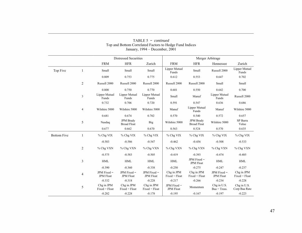
47

TABLE 5 − continued

Top and Bottom Correlated Factors to Hedge Fund Indices January, 1994 – December, 2001

Distressed Securities Merger Arbitrage FRM HFR Zurich FRM HFR Hennessee Zurich

Top Five 1 Small Small Small Lipper Mutual Funds Small Russell 2000 Lipper Mutual

Funds 0.809 0.753 0.775 0.612 0.553 0.647 0.702

2 Russell 2000 Russell 2000 Russell 2000 Russell 2000 Russell 2000 Small Small

0.800 0.750 0.770 0.601 0.550 0.642 0.700

3 Lipper Mutual Funds

Lipper Mutual Funds

Lipper Mutual Funds Small Manuf Lipper Mutual

Funds Russell 2000

0.732 0.706 0.720 0.591 0.547 0.636 0.686

4 Wilshire 5000 Wilshire 5000 Wilshire 5000 Manuf Lipper Mutual Funds Manuf Wilshire 5000

0.681 0.674 0.702 0.570 0.540 0.572 0.657

5 Nasdaq JPM Brady Broad Float Big Wilshire 5000 JPM Brady

Broad Float Wilshire 5000 SP Barra Value

0.677 0.662 0.670 0.563 0.524 0.570 0.635

Bottom Five 1 % Chg VIX % Chg VIX % Chg VIX % Chg VIX % Chg VIX % Chg VIX % Chg VIX

-0.583 -0.586 -0.547 -0.462 -0.456 -0.508 -0.533

2 % Chg VXN % Chg VXN % Chg VXN % Chg VXN % Chg VXN % Chg VXN % Chg VXN

-0.575 -0.583 -0.505 -0.419 -0.393 -0.474 -0.485

3 HML HML HML HML JPM Fixed − JPM Float HML HML

-0.390 -0.360 -0.338 -0.250 -0.275 -0.247 -0.237

4 JPM Fixed − JPM Float

JPM Fixed − JPM Float

JPM Fixed − JPM Float

Chg in JPM Fixed − Float

Chg in JPM Fixed − Float

JPM Fixed − JPM Float

Chg in JPM Fixed − Float

-0.332 -0.318 -0.228 -0.217 -0.266 -0.234 -0.228

5 Chg in JPM Fixed − Float

Chg in JPM Fixed − Float

Chg in JPM Fixed − Float

JPM Fixed − JPM Float Momentum Chg in U.S.

Baa − Treas. Chg in U.S.

Corp Baa Rate -0.282 -0.228 -0.178 -0.195 -0.167 -0.197 -0.223

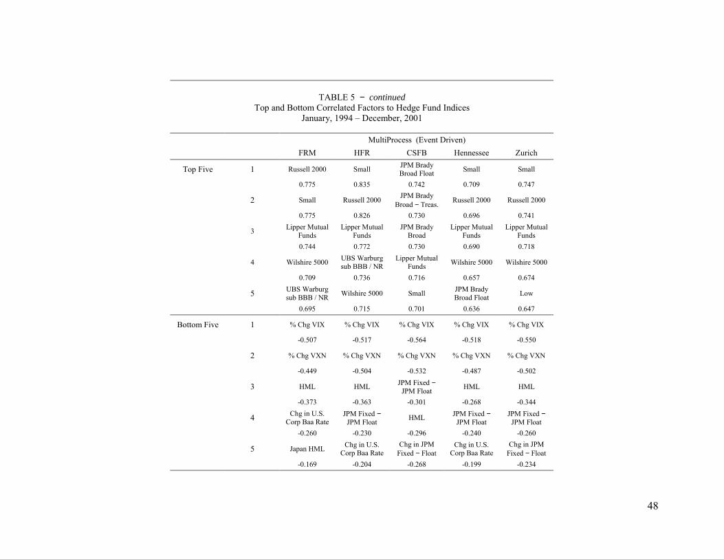
48

TABLE 5 − continued

Top and Bottom Correlated Factors to Hedge Fund Indices January, 1994 – December, 2001

MultiProcess (Event Driven) FRM HFR CSFB Hennessee Zurich

Top Five 1 Russell 2000 Small JPM Brady Broad Float Small Small

0.775 0.835 0.742 0.709 0.747

2 Small Russell 2000 JPM Brady Broad − Treas. Russell 2000 Russell 2000

0.775 0.826 0.730 0.696 0.741

3 Lipper Mutual Funds

Lipper Mutual Funds

JPM Brady Broad

Lipper Mutual Funds

Lipper Mutual Funds

0.744 0.772 0.730 0.690 0.718

4 Wilshire 5000 UBS Warburg sub BBB / NR

Lipper Mutual Funds Wilshire 5000 Wilshire 5000

0.709 0.736 0.716 0.657 0.674

5 UBS Warburg sub BBB / NR Wilshire 5000 Small JPM Brady

Broad Float Low

0.695 0.715 0.701 0.636 0.647

Bottom Five 1 % Chg VIX % Chg VIX % Chg VIX % Chg VIX % Chg VIX

-0.507 -0.517 -0.564 -0.518 -0.550

2 % Chg VXN % Chg VXN % Chg VXN % Chg VXN % Chg VXN

-0.449 -0.504 -0.532 -0.487 -0.502

3 HML HML JPM Fixed − JPM Float HML HML

-0.373 -0.363 -0.301 -0.268 -0.344

4 Chg in U.S. Corp Baa Rate

JPM Fixed − JPM Float HML JPM Fixed −

JPM Float JPM Fixed −

JPM Float -0.260 -0.230 -0.296 -0.240 -0.260

5 Japan HML Chg in U.S. Corp Baa Rate

Chg in JPM Fixed − Float

Chg in U.S. Corp Baa Rate

Chg in JPM Fixed − Float

-0.169 -0.204 -0.268 -0.199 -0.234

49

TABLE 6

Mapping of Hedge Fund Indices Using Only Index, French, and Interest Rate Factors January, 1994 – December, 2001

Int Factor 1 Factor 2 Factor 3 Factor 4 Factor 5 R^2 94 − 97

R^2 98 − 01

Arbitrage Convertible

FRM UBS

Warburg sub BBB / NR

0.2514 0.1220

coef: 0.0053 0.0062 t-stat: 3.4276 4.4922 inc. adj R^2: 0.1680

HFR SSB High Yield Index

UBS Warburg sub BBB / NR

Dow Jones Commodity 0.5047 0.5100

coef: 0.0036 0.0054 0.0049 0.0033 t-stat: 2.8865 4.3297 3.7409 2.8520 inc. adj R^2: 0.3279 0.4201 0.4614

CSFB SSB High Yield Index 0.2009 0.3017

coef: 0.0028 0.0111 t-stat: 1.1700 5.4324 inc. adj R^2: 0.2308

Henn UBS

Warburg sub BBB / NR

0.3999 0.3800

coef: 0.0011 0.0106 t-stat: 0.7329 7.7356 inc. adj R^2: 0.3825 Arbitrage

Fixed Income

FRM Lehman U.S. High Yield

Lehman U.S. Treasury

US Credit Bond 0.1036 0.4616

coef: 0.0062 0.0062 − 0.0216 0.0181 t-stat: 2.7561 2.3314 − 5.1961 3.5692 inc. adj R^2: 0.1951 0.3089 0.3864

HFR Chg in 10

Yr. US Swap Rate

Lehman Mortgage

Backed Secs

SSB High Yield Index

U.S. Real Estate − 0.0099 0.5750

coef: 0.0097 0.0209 0.0145 0.0063 − 0.0047 t-stat: 3.9831 7.1353 5.0697 3.8844 − 2.9352 inc. adj R^2: 0.0978 0.3095 0.3550 0.4043

CSFB CME Yen Futures

Lehman U.S. High Yield 0.1875 0.3193

coef: 0.0030 − 0.0065 0.0063 t-stat: 1.6733 − 4.3337 4.2798 inc. adj R^2: 0.1425 0.2759

Credit Trading

FRM SSB High Yield Index

JPM Brady Broad Fixed Utils 0.3657 0.5039

coef: 0.0014 0.0090 0.0081 − 0.0045 t-stat: 0.7735 4.8513 3.6629 − 2.6876 inc. adj R^2: 0.3686 0.4217 0.4580

HFR SSB High Yield Index

JPM Fixed − JPM Float

Chg in U.S. High Yld

Ind − Treas.

Chg in 10 Yr. US

Swap Rate

US Credit Bond 0.7243 0.7986

coef: 0.0015 0.0114 − 0.0014 0.0044 0.0105 0.0065 t-stat: 1.1562 9.6687 − 1.0031 3.6936 4.7327 3.0569 inc. adj R^2: 0.6120 0.7034 0.7221 0.7524 0.7732

50

TABLE 6 − continued

Mapping of Hedge Fund Indices Using Only Index, French, and Interest Rate Factors January, 1994 – December, 2001

Int Factor 1 Factor 2 Factor 3 Factor 4 Factor 5 R^2 94 − 97

R^2 98 − 01

Distressed Securities

FRM Small SSB High Yield Index

JPM Fixed − JPM Float

Chg in UBS Global −

Treas

JPM Brady Broad Fixed

0.5704 0.7769

coef: 0.0024 0.0076 0.0045 − 0.0047 0.0037 0.0040 t-stat: 2.1040 5.5665 3.5358 − 4.3205 2.9980 2.6896 inc. adj R^2: 0.5721 0.6294 0.6698 0.6983 0.7177

HFR Small JPM Brady Broad Float

Chg in UBS Global −

Treas. 0.6216 0.6191

coef: 0.0011 0.0102 0.0065 0.0051 t-stat: 0.7093 5.7433 3.5316 3.0780 inc. adj R^2: 0.5207 0.5747 0.6102

Zurich Small SSB High Yield Index 0.6795 0.6644

coef: 0.0005 0.0152 0.0056 t-stat: 0.3040 9.6139 3.6835 inc. adj R^2: 0.6189 0.6638

Merger Arbitrage

FRM Small Hlth 0.3708 0.4462

coef: 0.0048 0.0049 0.0032 t-stat: 5.1244 5.5430 3.4892 inc. adj R^2: 0.3401 0.4102

HFR Small Hlth Momentum 0.0375 0.4709

coef: 0.0048 0.0043 0.0031 − 0.0024 t-stat: 4.8509 4.6243 3.1930 − 2.7543 inc. adj R^2: 0.2594 0.3081 0.3539

Hennessee Small Hlth 0.3894 0.4336

coef: 0.0040 0.0046 0.0022 t-stat: 4.8311 5.9782 2.7976 inc. adj R^2: 0.3610 0.4043

Zurich Small SP Barra Value 0.4687 0.5105

coef: 0.0038 0.0056 0.0033 t-stat: 4.1175 5.5077 3.1887 inc. adj R^2: 0.4414 0.4910

51

TABLE 6 − continued

Mapping of Hedge Fund Indices Using Only Index, French, and Interest Rate Factors January, 1994 – December, 2001

Int Factor 1 Factor 2 Factor 3 Factor 4 Factor 5 R^2 94 − 97

R^2 98 − 01

MultiProcess(Event Driven)

FRM UBS

Warburg sub BBB / NR

Lipper Mutual Funds

JPM Brady Broad SMB HiTec 0.6786 0.7872

coef: 0.0067 0.0065 0.0100 0.0036 0.0038 − 0.0058 t-stat: 6.0896 4.1120 5.1673 2.7015 3.7883 − 3.5592 inc. adj R^2: 0.5783 0.6451 0.6721 0.6968 0.7312

HFR Small JPM Brady Broad Fixed

UBS Warburg

AAA / AA 0.4889 0.7888

coef: 0.0037 0.0115 0.0058 0.0038 t-stat: 2.9355 8.9383 4.1595 3.1280 inc. adj R^2: 0.6087 0.6673 0.6960

CSFB JPM Brady Ind. − Treas. Small SSB High

Yield Index MSCI 10

Yr +

Chg in UBS Global Ind.

− Treas. 0.5880 0.6799

coef: 0.0023 0.0090 0.0051 0.0061 − 0.0047 0.0049 t-stat: 1.4340 4.4835 2.7219 3.5358 − 3.1348 2.8593 inc. adj R^2: 0.4286 0.5471 0.5838 0.6133 0.6416

Hennessee Small JPM Brady Broad Fixed 0.3008 0.5576

coef: 0.0030 0.0091 0.0073 t-stat: 1.8677 5.5156 3.9733 inc. adj R^2: 0.3933 0.4758

Zurich Small Chg in U.S. High Yld.

Ind. − Treas. 0.3535 0.6308

coef: 0.0031 0.0082 0.0037 t-stat: 2.9362 8.1162 3.6981 inc. adj R^2: 0.4808 0.5425

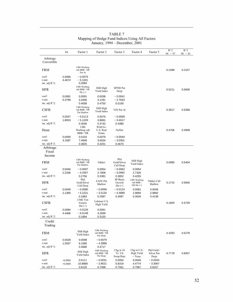
52

TABLE 7

Mapping of Hedge Fund Indices Using All Factors January, 1994 – December, 2001

Int Factor 1 Factor 2 Factor 3 Factor 4 Factor 5 R^2 94 − 97

R^2 98 − 01

Arbitrage Convertible

FRM UBS Warburg sub BBB / NR

Put At 0.2288 0.2157

coef: 0.0066 − 0.0075 t-stat: 4.4674 − 5.1001 inc. adj R^2: 0.2084

HFR UBS Warburg sub BBB / NR

Dir (−)

SSB High Yield Index

SP500 Put Deep 0.5211 0.5606

coef: 0.0081 0.0091 0.0038 − 0.0041 t-stat: 5.3799 3.3306 3.1281 − 2.7633 inc. adj R^2: 0.4058 0.4750 0.5100

CSFB UBS Warburg sub BBB / NR Put Shallow

SSB High Yield Index VIX Put At 0.3517 0.5358

coef: 0.0037 − 0.0113 0.0076 − 0.0069 t-stat: 1.8053 − 5.1229 3.8691 − 3.4017 inc. adj R^2: 0.3046 0.3742 0.4380

Henn UBS

Warburg sub BBB / NR

Wrld Ex-U.S. Real

Estate NoDur 0.4706 0.4908

coef: 0.0059 0.0103 0.0079 − 0.0044 t-stat: 3.1587 7.4949 3.6034 − 3.0301 inc. adj R^2: 0.3825 0.4201 0.4670 Arbitrage

Fixed Income

FRM UBS Warburg sub BBB / NR Put Shallow

Nikkei Phil

Gold/Silver Call Deep

SSB High Yield Index 0.0085 0.5404

coef: 0.0046 − 0.0097 0.0054 − 0.0062 0.0054 t-stat: 2.2336 − 4.3357 2.7808 − 3.0992 2.7326 inc. adj R^2: 0.2756 0.3381 0.3852 0.4255

HFR Phil

Gold/Silver Call Deep

EAFE Put Shallow

SP Barra Growth Dir (+)

UBS Warburg sub BBB / NR Dir (+)

Nikkei Call Shallow 0.1710 0.5840

coef: 0.0049 − 0.0080 − 0.0056 − 0.0124 0.0081 0.0046 t-stat: 2.1385 − 5.2221 − 3.5134 − 4.4889 2.9894 2.9892 inc. adj R^2: 0.1863 0.2587 0.3087 0.3626 0.4138

CSFB CME Yen

Futures Dir (+)

Lehman U.S. High Yield 0.1829 0.3729

coef: 0.0084 − 0.0126 0.0061 t-stat: 4.4466 − 5.0148 4.2699 inc. adj R^2: 0.1894 0.3150

Credit Trading

FRM SSB High Yield Index

UBS Warburg sub BBB / NR

Put Deep 0.3250 0.5278

coef: 0.0028 0.0098 − 0.0079 t-stat: 1.5937 6.1585 − 4.3989 inc. adj R^2: 0.3686 0.4717

HFR SSB High Yield Index

UBS Warburg sub BBB / NR

Put Deep

Chg in 10 Yr. US

Swap Rate

Chg in U.S. High Yield

− Treas.

Phil Gold / Silver Put

Deep 0.7778 0.8357

coef: −0.0002 0.0111 − 0.0031 0.0054 0.0045 − 0.0034 t-stat: −0.2504 10.8868 − 2.9021 5.8319 4.4774 − 3.3067 inc. adj R^2: 0.6120 0.7068 0.7561 0.7967 0.8167

53

TABLE 7 − continued

Mapping of Hedge Fund Indices Using All Factors January, 1994 – December, 2001

Int Factor 1 Factor 2 Factor 3 Factor 4 Factor 5 R^2 94 − 97

R^2 98 − 01

Distressed Securities

FRM UBS Warburg sub BBB / NR

Put At Small VIX Call

Deep

UBS Warburg sub BBB / NR Dir (−)

SSB High Yield Index

0.5596 0.8491

coef: −0.0012 − 0.0127 0.0088 − 0.0036 − 0.0142 0.0031 t-stat: −0.6014 − 5.1373 6.7764 − 2.9152 − 3.2286 2.9219 inc. adj R^2: 0.5795 0.7036 0.7360 0.7535 0.7724

HFR UBS Warburg sub BBB / NR

Put At Small

UBS Warburg sub BBB / NR Dir (−)

VIX Call Deep

Salomon WGBI Put Shallow

0.6199 0.7912

coef: −0.0026 − 0.0162 0.0099 − 0.0177 − 0.0058 − 0.0037 t-stat: −1.0950 − 5.3215 6.1948 − 3.2873 − 3.7787 − 2.9311 inc. adj R^2: 0.5487 0.6532 0.6928 0.7207 0.7422

Zurich Small UBS Warburg sub BBB / NR

Put Deep

Chg in U.S. High Yield

− Treas.

Europe HML 0.6611 0.8598

coef: 0.0025 0.0139 − 0.0086 0.0036 0.0028 t-stat: 1.9619 10.9207 − 6.5710 3.0341 2.6556 inc. adj R^2: 0.6189 0.7362 0.7606 0.7754

Merger Arbitrage

FRM UBS Warburg sub BBB / NR

Put At

UBS Warburg AAA / AA

Dir (+)

EAFE Put Deep 0.3506 0.6367

coef: 0.0049 − 0.0051 0.0038 − 0.0030 t-stat: 4.7900 − 5.3108 3.3493 − 3.1623 inc. adj R^2: 0.4190 0.4781 0.5241

HFR UBS Warburg sub BBB / NR

Put At EAFE Put

Deep − 0.0131 0.5873

coef: 0.0065 − 0.0045 − 0.0039 t-stat: 7.3344 − 4.3459 − 3.7366 inc. adj R^2: 0.3528 0.4312

Hennessee UBS Warburg sub BBB / NR

Put At VIX Call At

UBS Warburg AAA / AA

Dir (+) 0.4413 0.5943

coef: 0.0046 − 0.0045 − 0.0029 0.0026 t-stat: 5.1053 − 5.4683 − 3.5397 2.6626 inc. adj R^2: 0.4413 0.5105 0.5406

Zurich UBS Warburg sub BBB / NR

Put At VIX Call At

U.S. Real Estate Call

Deep Small 0.6283 0.7073

coef: 0.0053 − 0.0048 − 0.0035 0.0022 0.0026 t-stat: 6.9490 − 4.7748 − 3.9380 2.9718 2.9331 inc. adj R^2: 0.5228 0.6005 0.6433 0.6706

54

TABLE 7 − continued

Mapping of Hedge Fund Indices Using All Factors January, 1994 – December, 2001

Int Factor 1 Factor 2 Factor 3 Factor 4 Factor 5 R^2 94 − 97

R^2 98 − 01

MultiProcess(Event Driven)

FRM UBS

Warburg sub BBB / NR

VIX Call At Small NASDAQ EAFE Put Deep 0.6832 0.8209

coef: 0.0078 0.0093 − 0.0035 0.0106 − 0.0081 − 0.0043 t-stat: 7.3212 5.7979 − 2.7075 5.4002 − 3.8480 − 3.6557 inc. adj R^2: 0.5783 0.6498 0.6824 0.7158 0.7498

HFR Small UBS Warburg sub BBB / NR

Put At

UBS Warburg AAA / AA

Dir (+)

JPM Brady Broad Fixed

0.5119 0.8717

coef: 0.0022 0.0079 − 0.0072 0.0060 0.0040 t-stat: 1.6354 5.8624 − 5.0407 3.7844 3.0798 inc. adj R^2: 0.6087 0.7041 0.7389 0.7610

CSFB UBS Warburg sub BBB / NR

Put At JPM Brady

Broad Europe

High BM

UBS Warburg sub BBB / NR Dir (−)

UBS Warburg sub BBB / NR Call At

0.5924 0.8972

coef: −0.0076 −0.0269 0.0072 0.0039 −0.0266 0.0046 t-stat: −3.5288 −10.4792 5.1674 3.4199 −5.5171 3.4892 inc. adj R^2: 0.6571 0.7219 0.7576 0.7969 0.8191

Hennessee UBS Warburg sub BBB / NR

Put At

U.S. Real Estate Call

Deep VIX Call At

UBS Warburg sub BBB / NR Call At

Pacific Rim HML 0.4765 0.7325

coef: 0.0028 −0.0001 0.0053 −0.0030 0.0037 −0.0056 t-stat: 2.5568 −0.0541 4.5413 −2.8725 2.9826 −2.7124 inc. adj R^2: 0.4705 0.5375 0.5871 0.6128 0.6401

Zurich UBS Warburg sub BBB / NR

Put At Russell 2000 VIX Call

Shallow UBS Warburg

AAA / AA Dir (+)

UBS Warburg sub BBB /

NR Put Deep 0.5129 0.8029

coef: 0.0028 − 0.0001 0.0053 − 0.0030 0.0037 − 0.0056 t-stat: 2.5568 − 0.0541 4.5413 − 2.8725 2.9826 − 2.7124 inc. adj R^2: 0.5275 0.6219 0.6597 0.6839 0.7045

55

TABLE 8

Index Factors Value-at-Risk Estimation

Index Factors Six Month Analysis One Year Analysis

50,000 simulations Mean Std Dev Min 1 Percentile

5 Percentile Mean Std Dev Min 1

Percentile 5

Percentile SP500 4.68 11.09 -43.09 -21.25 -13.63 9.82 16.52 -48.37 -26.07 -16.42 DJIA 5.10 11.61 -42.78 -21.52 -13.96 10.37 17.11 -50.60 -26.62 -16.80 NASDAQ 5.26 21.85 -64.56 -39.97 -28.58 10.92 33.04 -74.62 -49.51 -36.57 Russell 2000 2.79 13.97 -49.46 -28.90 -19.72 5.48 20.37 -56.68 -36.42 -25.82 Wilshire 5000 3.54 11.33 -40.08 -23.16 -15.34 7.08 16.62 -51.46 -29.09 -19.43 SP Barra Growth 4.48 12.64 -41.34 -24.27 -16.11 9.20 18.82 -49.25 -30.06 -20.06 SP Barra Value 3.01 10.66 -44.46 -22.21 -14.77 6.22 15.68 -47.40 -27.91 -18.52 MSCI World 2.22 10.01 -37.22 -21.19 -14.32 4.53 14.58 -46.74 -27.06 -18.50 Nikkei -4.00 14.20 -48.19 -32.45 -25.44 -7.64 19.43 -64.10 -44.07 -35.94 FTSE 0.82 9.44 -32.68 -21.02 -14.69 1.49 13.43 -47.44 -27.10 -19.75 EAFE -0.10 10.27 -39.54 -23.10 -16.76 -0.33 14.58 -50.10 -30.89 -22.91 Lipper Mut Funds 3.79 10.97 -41.25 -22.44 -14.57 7.66 16.16 -48.13 -27.91 -18.11 MSCI AAA -0.61 6.71 -24.24 -14.46 -10.87 -1.29 9.41 -32.82 -20.46 -15.55 MSCI 10 Yr + 1.30 5.82 -20.31 -11.81 -8.15 2.66 8.27 -28.70 -15.50 -10.42 MSCI Wld Sov Ex-USA -0.57 5.62 -23.91 -12.62 -9.32 -1.14 7.92 -30.17 -17.67 -13.34 UBS Warburg AAA / AA 4.18 9.10 -34.22 -15.58 -9.83 8.43 13.32 -38.14 -18.89 -11.78 UBS Warburg sub BBB / NR 4.55 15.11 -48.50 -27.20 -18.69 9.18 22.28 -60.85 -34.57 -23.52 CBT Municipal Bond -2.51 5.37 -28.16 -15.12 -11.33 -4.91 7.45 -39.01 -21.62 -16.99 Leh Bros Gov/Corp 0.80 2.25 -7.87 -4.34 -2.85 1.58 3.24 -10.82 -5.73 -3.66 US Credit Bond -2.64 3.38 -15.35 -10.43 -8.17 -5.10 4.67 -23.11 -15.54 -12.62 Salomon WGBI -0.27 4.22 -17.71 -9.33 -6.92 -0.48 5.95 -22.67 -13.26 -9.74 CME Goldman Commodity -0.33 12.91 -40.71 -25.81 -19.45 -0.56 18.28 -51.14 -35.15 -26.89 Dow Jones Commodity -3.55 12.13 -66.89 -43.03 -33.19 -6.98 16.65 -80.39 -50.83 -41.07 Philadelphia Gold / Silver -2.86 25.42 -65.95 -46.73 -37.16 -5.56 35.61 -79.38 -60.09 -49.90 Wld Ex-US Real Estate -0.86 14.72 -59.14 -36.17 -25.19 -1.76 20.66 -71.94 -45.60 -33.86 U.S. Real Estate 2.45 12.33 -40.28 -24.38 -17.02 4.93 17.91 -51.50 -31.16 -22.19 CME Yen Futures -2.86 9.51 -32.80 -21.04 -16.49 -5.52 13.21 -45.55 -29.90 -24.24 NYBOT Dollar Index -0.95 5.16 -21.07 -12.26 -9.11 -1.84 7.28 -27.15 -17.49 -13.22 NYBOT Orange Juice -1.01 21.31 -64.08 -41.72 -31.82 -1.65 30.13 -74.32 -53.52 -42.77

56

TABLE 9

Ken French Factors Value-at-Risk Estimation

Index Factors Six Month Analysis One Year Analysis

50,000 simulations Mean Std Dev Min 1 Percentile

5 Percentile Mean Std Dev Min 1

Percentile 5

Percentile SMB -1.89 9.59 -35.49 -21.67 -16.30 -3.82 13.28 -42.80 -30.09 -23.37 HML -2.39 11.67 -50.91 -31.44 -22.62 -4.74 16.12 -66.99 -40.62 -30.67 Low 4.60 12.31 -42.01 -23.61 -15.77 9.35 18.26 -54.23 -29.50 -19.47 High 4.32 10.06 -37.94 -17.89 -11.77 8.84 15.00 -45.03 -22.49 -14.36 Big 4.62 11.29 -43.58 -21.86 -14.00 9.33 16.80 -54.30 -27.19 -17.35 Small 4.32 14.91 -52.45 -29.24 -19.70 9.05 22.12 -60.07 -36.52 -24.73 Momentum 3.55 13.70 -55.56 -30.65 -19.40 7.09 20.16 -63.66 -37.10 -24.64 Europe High BM 5.46 13.53 -50.76 -25.95 -16.79 11.05 20.41 -55.74 -32.18 -20.57 Europe Low BM 2.42 11.51 -41.65 -23.11 -16.10 4.91 16.74 -57.93 -29.86 -20.97 Europe HML 0.60 8.07 -39.68 -18.68 -12.59 1.13 11.48 -45.80 -24.40 -17.18 UK High BM 2.93 11.56 -38.66 -22.80 -15.64 6.03 16.96 -48.87 -29.01 -20.08 UK Low BM 2.51 9.71 -33.17 -19.06 -13.15 5.00 14.20 -40.52 -25.02 -17.30 UK HML -1.79 8.61 -35.12 -21.13 -15.36 -3.55 11.88 -42.54 -28.76 -22.04 Pacific Rim High BM 0.68 18.34 -46.53 -32.15 -24.71 1.17 26.39 -62.15 -43.12 -34.03 Pacific Rim Low BM -4.53 13.51 -47.15 -31.39 -25.02 -8.80 18.37 -60.81 -43.30 -35.49 Pacific Rim HML 3.00 12.90 -48.59 -24.46 -16.73 5.79 18.92 -51.14 -31.40 -21.93 Japan High BM 1.24 21.16 -52.11 -34.89 -27.21 2.90 30.81 -62.41 -47.03 -36.83 Japan Low BM -4.81 14.98 -48.91 -33.77 -26.97 -9.49 20.19 -62.51 -46.25 -38.14 Japan HML 4.21 15.61 -47.22 -27.01 -18.77 8.33 22.87 -53.33 -34.22 -23.98 NoDurbl 3.94 10.29 -37.81 -19.69 -12.83 8.10 15.08 -46.03 -24.35 -15.67 Durbl 5.48 14.46 -39.47 -24.55 -16.68 11.29 21.72 -56.39 -31.21 -20.88 Manuf 3.09 10.89 -46.44 -21.96 -14.57 6.23 15.98 -53.93 -28.02 -18.78 Enrgy 3.93 12.70 -33.89 -21.20 -14.94 7.95 18.73 -45.90 -27.42 -19.28 HiTec 8.69 23.79 -63.03 -39.99 -27.97 18.07 37.23 -75.36 -48.84 -34.86 Telcm 2.24 16.13 -52.43 -32.26 -22.97 4.63 23.54 -64.64 -41.67 -30.27 Shops 4.58 12.07 -38.96 -21.60 -14.44 9.18 18.02 -47.35 -27.34 -18.20 Hlth 7.71 12.30 -39.27 -19.35 -12.08 16.06 18.90 -46.20 -23.13 -13.14 Utils 2.55 10.82 -34.46 -20.45 -14.35 5.12 15.71 -47.13 -26.47 -18.77 Other 5.19 12.26 -46.45 -24.34 -14.85 10.50 18.39 -57.02 -29.64 -18.51

57

TABLE 10 Value-at-Risk Estimation

Excess Returns

Six Month Analysis One Year Analysis

50,000 simulations Mean Std Dev Min 1 Percentile

5 Percentile Mean Std Dev Min 1

Percentile 5

Percentile Arbitrage Convertible FRM Index, French Normal 4.09 4.14 -11.14 -5.20 -2.63 8.34 6.10 -17.37 -5.22 -1.40 T-dist 4.10 5.63 -71.06 -9.12 -4.71 8.28 8.22 -50.33 -10.44 -4.68 All Normal 4.08 4.14 -14.31 -5.98 -2.79 8.31 6.10 -18.32 -5.93 -1.65 T-dist 4.04 5.53 -37.21 -9.55 -4.94 8.31 8.21 -52.34 -10.63 -4.68 Historical 4.05 4.10 -15.82 -5.62 -2.63 8.33 6.05 -16.55 -5.46 -1.46 HFR Index, French Normal 3.06 4.06 -13.64 -6.42 -3.64 6.19 5.91 -17.96 -7.26 -3.34 T-dist 3.07 5.04 -43.26 -8.80 -5.04 6.25 7.33 -56.24 -10.38 -5.42 All Normal 3.06 4.02 -16.26 -7.16 -3.86 6.19 5.89 -18.87 -7.94 -3.70 T-dist 3.06 4.91 -31.81 -8.94 -5.08 6.17 7.16 -44.28 -10.57 -5.43 Historical 3.11 3.87 -16.93 -7.32 -3.80 6.26 5.66 -21.35 -7.92 -3.42 CSFB Index, French Normal 2.90 6.60 -24.06 -11.74 -7.67 5.95 9.66 -29.45 -14.88 -9.21 T-dist 2.99 8.78 -99.61 -17.06 -10.72 6.07 12.76 -97.37 -21.67 -13.69 All Normal 2.93 6.66 -29.81 -14.36 -8.56 5.99 9.66 -35.24 -17.17 -10.05 T-dist 2.96 8.28 -72.27 -17.33 -10.60 5.90 12.03 -57.70 -21.66 -13.14 Historical 2.93 7.27 -31.81 -16.42 -9.77 5.96 10.57 -44.07 -19.54 -11.67 Henn Index, French Normal 2.07 4.68 -15.71 -8.32 -5.42 4.22 6.80 -20.40 -10.61 -6.60 T-dist 2.15 5.98 -45.26 -11.68 -7.24 4.30 8.67 -99.74 -15.24 -9.27 All Normal 2.09 4.68 -17.11 -8.86 -5.59 4.27 6.79 -21.95 -11.09 -6.71 T-dist 2.09 5.81 -76.74 -11.56 -7.26 4.27 8.39 -49.07 -14.82 -9.03 Historical 2.18 4.52 -18.58 -9.18 -5.48 4.40 6.48 -22.72 -10.95 -6.30

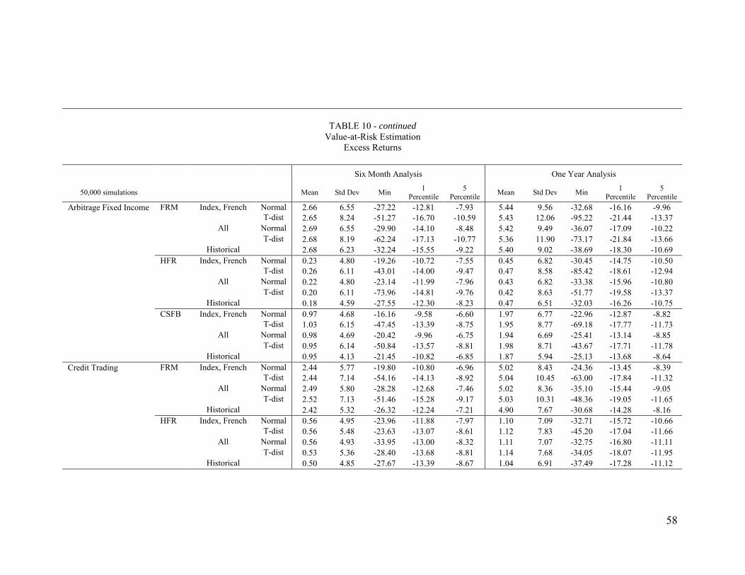
58

TABLE 10 - continued Value-at-Risk Estimation

Excess Returns

Six Month Analysis One Year Analysis

50,000 simulations Mean Std Dev Min 1 Percentile

5 Percentile Mean Std Dev Min 1

Percentile 5

Percentile Arbitrage Fixed Income FRM Index, French Normal 2.66 6.55 -27.22 -12.81 -7.93 5.44 9.56 -32.68 -16.16 -9.96 T-dist 2.65 8.24 -51.27 -16.70 -10.59 5.43 12.06 -95.22 -21.44 -13.37 All Normal 2.69 6.55 -29.90 -14.10 -8.48 5.42 9.49 -36.07 -17.09 -10.22 T-dist 2.68 8.19 -62.24 -17.13 -10.77 5.36 11.90 -73.17 -21.84 -13.66 Historical 2.68 6.23 -32.24 -15.55 -9.22 5.40 9.02 -38.69 -18.30 -10.69 HFR Index, French Normal 0.23 4.80 -19.26 -10.72 -7.55 0.45 6.82 -30.45 -14.75 -10.50 T-dist 0.26 6.11 -43.01 -14.00 -9.47 0.47 8.58 -85.42 -18.61 -12.94 All Normal 0.22 4.80 -23.14 -11.99 -7.96 0.43 6.82 -33.38 -15.96 -10.80 T-dist 0.20 6.11 -73.96 -14.81 -9.76 0.42 8.63 -51.77 -19.58 -13.37 Historical 0.18 4.59 -27.55 -12.30 -8.23 0.47 6.51 -32.03 -16.26 -10.75 CSFB Index, French Normal 0.97 4.68 -16.16 -9.58 -6.60 1.97 6.77 -22.96 -12.87 -8.82 T-dist 1.03 6.15 -47.45 -13.39 -8.75 1.95 8.77 -69.18 -17.77 -11.73 All Normal 0.98 4.69 -20.42 -9.96 -6.75 1.94 6.69 -25.41 -13.14 -8.85 T-dist 0.95 6.14 -50.84 -13.57 -8.81 1.98 8.71 -43.67 -17.71 -11.78 Historical 0.95 4.13 -21.45 -10.82 -6.85 1.87 5.94 -25.13 -13.68 -8.64 Credit Trading FRM Index, French Normal 2.44 5.77 -19.80 -10.80 -6.96 5.02 8.43 -24.36 -13.45 -8.39 T-dist 2.44 7.14 -54.16 -14.13 -8.92 5.04 10.45 -63.00 -17.84 -11.32 All Normal 2.49 5.80 -28.28 -12.68 -7.46 5.02 8.36 -35.10 -15.44 -9.05 T-dist 2.52 7.13 -51.46 -15.28 -9.17 5.03 10.31 -48.36 -19.05 -11.65 Historical 2.42 5.32 -26.32 -12.24 -7.21 4.90 7.67 -30.68 -14.28 -8.16 HFR Index, French Normal 0.56 4.95 -23.96 -11.88 -7.97 1.10 7.09 -32.71 -15.72 -10.66 T-dist 0.56 5.48 -23.63 -13.07 -8.61 1.12 7.83 -45.20 -17.04 -11.66 All Normal 0.56 4.93 -33.95 -13.00 -8.32 1.11 7.07 -32.75 -16.80 -11.11 T-dist 0.53 5.36 -28.40 -13.68 -8.81 1.14 7.68 -34.05 -18.07 -11.95 Historical 0.50 4.85 -27.67 -13.39 -8.67 1.04 6.91 -37.49 -17.28 -11.12

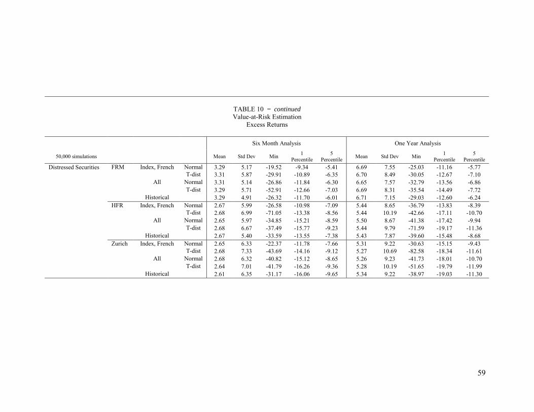
59

TABLE 10 − continued Value-at-Risk Estimation

Excess Returns

Six Month Analysis One Year Analysis

50,000 simulations Mean Std Dev Min 1 Percentile

5 Percentile Mean Std Dev Min 1

Percentile 5

Percentile Distressed Securities FRM Index, French Normal 3.29 5.17 -19.52 -9.34 -5.41 6.69 7.55 -25.03 -11.16 -5.77 T-dist 3.31 5.87 -29.91 -10.89 -6.35 6.70 8.49 -30.05 -12.67 -7.10 All Normal 3.31 5.14 -26.86 -11.84 -6.30 6.65 7.57 -32.79 -13.56 -6.86 T-dist 3.29 5.71 -52.91 -12.66 -7.03 6.69 8.31 -35.54 -14.49 -7.72 Historical 3.29 4.91 -26.32 -11.70 -6.01 6.71 7.15 -29.03 -12.60 -6.24 HFR Index, French Normal 2.67 5.99 -26.58 -10.98 -7.09 5.44 8.65 -36.79 -13.83 -8.39 T-dist 2.68 6.99 -71.05 -13.38 -8.56 5.44 10.19 -42.66 -17.11 -10.70 All Normal 2.65 5.97 -34.85 -15.21 -8.59 5.50 8.67 -41.38 -17.42 -9.94 T-dist 2.68 6.67 -37.49 -15.77 -9.23 5.44 9.79 -71.59 -19.17 -11.36 Historical 2.67 5.40 -33.59 -13.55 -7.38 5.43 7.87 -39.60 -15.48 -8.68 Zurich Index, French Normal 2.65 6.33 -22.37 -11.78 -7.66 5.31 9.22 -30.63 -15.15 -9.43 T-dist 2.68 7.33 -43.69 -14.16 -9.12 5.27 10.69 -82.58 -18.34 -11.61 All Normal 2.68 6.32 -40.82 -15.12 -8.65 5.26 9.23 -41.73 -18.01 -10.70 T-dist 2.64 7.01 -41.79 -16.26 -9.36 5.28 10.19 -51.65 -19.79 -11.99 Historical 2.61 6.35 -31.17 -16.06 -9.65 5.34 9.22 -38.97 -19.03 -11.30

60

TABLE 10 − continued Value-at-Risk Estimation

Excess Returns

Six Month Analysis One Year Analysis

50,000 simulations Mean Std Dev Min 1 Percentile

5 Percentile Mean Std Dev Min 1

Percentile 5

Percentile Merger Arbitrage FRM Index, French Normal 4.14 2.89 -7.05 -2.50 -0.57 8.44 4.27 -9.87 -1.29 1.49 T-dist 4.10 3.63 -20.01 -4.51 -1.70 8.43 5.36 -31.35 -3.97 -0.16 All Normal 4.12 2.89 -12.64 -4.13 -1.02 8.40 4.28 -12.57 -2.81 0.97 T-dist 4.13 3.52 -30.46 -5.17 -1.86 8.39 5.14 -17.72 -4.32 -0.25 Historical 4.10 3.02 -17.83 -4.67 -1.66 8.39 4.48 -19.19 -3.83 0.33 HFR Index, French Normal 3.76 2.90 -7.37 -2.87 -1.00 7.67 4.26 -8.86 -2.00 0.77 T-dist 3.74 3.72 -32.51 -5.04 -2.21 7.68 5.45 -32.75 -4.75 -0.99 All Normal 3.76 2.88 -12.83 -4.40 -1.40 7.63 4.23 -14.64 -3.40 0.25 T-dist 3.75 3.63 -24.77 -5.83 -2.40 7.66 5.31 -26.12 -5.36 -1.08 Historical 3.71 3.36 -16.20 -6.68 -2.98 7.62 4.94 -26.95 -6.14 -1.46 Henn Index, French Normal 3.37 2.50 -7.45 -2.44 -0.75 6.87 3.67 -7.54 -1.42 0.89 T-dist 3.39 3.17 -21.71 -4.16 -1.68 6.88 4.62 -15.19 -3.90 -0.54 All Normal 3.37 2.50 -10.29 -3.50 -1.05 6.89 3.67 -11.42 -2.68 0.58 T-dist 3.38 3.04 -14.27 -4.61 -1.80 6.88 4.40 -39.41 -4.00 -0.51 Historical 3.38 2.88 -13.75 -5.17 -2.16 6.83 4.23 -17.04 -4.78 -0.79 Zurich Index, French Normal 3.34 3.15 -10.43 -4.04 -1.84 6.76 4.59 -11.55 -3.68 -0.75 T-dist 3.32 3.85 -38.08 -5.86 -2.88 6.77 5.65 -33.75 -6.28 -2.23 All Normal 3.31 3.14 -15.54 -5.38 -2.26 6.78 4.58 -20.12 -4.77 -1.20 T-dist 3.36 3.60 -19.01 -6.14 -2.85 6.83 5.27 -23.25 -6.29 -2.04 Historical 3.34 3.32 -17.53 -6.86 -3.21 6.80 4.83 -21.75 -6.93 -2.03

61

TABLE 10 − continued Value-at-Risk Estimation

Excess Returns

Six Month Analysis One Year Analysis

50,000 simulations Mean Std Dev Min 1 Percentile

5 Percentile Mean Std Dev Min 1

Percentile 5

Percentile FRM Index, French Normal 5.48 4.97 -14.69 -6.04 -2.66 11.19 7.48 -18.30 -5.75 -0.96 MultiProcess

(Event Driven) T-dist 5.49 5.57 -32.92 -7.28 -3.60 11.18 8.38 -26.78 -7.65 -2.16 All Normal 5.46 4.97 -22.06 -7.10 -3.00 11.26 7.41 -20.37 -6.34 -1.12 T-dist 5.48 5.57 -28.54 -8.27 -3.91 11.20 8.36 -40.35 -8.47 -2.43 Historical 5.49 5.42 -24.09 -8.88 -3.70 11.30 8.05 -27.34 -8.05 -2.04 HFR Index, French Normal 4.83 5.46 -16.85 -7.90 -4.15 9.86 8.05 -19.00 -8.16 -3.11 T-dist 4.77 6.21 -37.58 -9.66 -5.27 9.75 9.18 -43.40 -10.85 -4.90 All Normal 4.80 5.44 -23.32 -9.25 -4.48 9.86 8.06 -25.68 -9.64 -3.65 T-dist 4.81 6.02 -35.74 -10.09 -5.30 9.83 8.96 -50.27 -11.43 -4.87 Historical 4.80 5.38 -23.33 -10.21 -4.61 9.84 8.05 -29.88 -10.51 -3.94 CSFB Index, French Normal 3.35 6.42 -25.67 -12.26 -7.45 6.80 9.31 -31.45 -14.24 -8.34 T-dist 3.33 7.38 -41.63 -14.23 -8.74 6.84 11.00 -58.39 -17.83 -10.70 All Normal 3.42 6.32 -36.23 -17.44 -9.85 6.73 9.38 -42.40 -19.60 -11.78 T-dist 3.33 6.96 -38.27 -18.28 -10.61 6.80 10.09 -45.44 -20.67 -12.11 Historical 3.33 6.47 -36.21 -18.59 -12.45 6.85 9.41 -45.03 -20.38 -12.72 Henn Index, French Normal 3.76 5.45 -19.05 -8.74 -5.14 7.68 7.98 -19.65 -10.07 -5.11 T-dist 3.83 6.67 -51.35 -11.73 -6.86 7.67 9.87 -67.22 -14.10 -7.86 All Normal 3.78 5.46 -21.96 -10.80 -5.56 7.67 8.05 -32.66 -11.82 -5.92 T-dist 3.80 6.35 -39.64 -12.28 -6.86 7.70 9.29 -49.14 -14.34 -7.52 Historical 3.79 6.05 -32.64 -13.44 -6.98 7.75 8.89 -33.75 -14.52 -7.58 Zurich Index, French Normal 2.79 3.79 -13.20 -5.97 -3.42 5.69 5.49 -18.34 -6.65 -3.20 T-dist 2.83 4.57 -56.39 -7.79 -4.55 5.68 6.61 -41.37 -9.31 -4.93 All Normal 2.79 3.77 -20.86 -8.50 -4.23 5.70 5.49 -22.09 -8.94 -4.10 T-dist 2.81 4.28 -46.74 -9.06 -4.77 5.67 6.25 -29.30 -10.46 -5.06 Historical 2.80 4.04 -22.47 -9.89 -5.20 5.71 5.84 -23.12 -10.50 -5.14