Heavy Quark Effective Field Theory∗†

Howard GeorgiLyman Laboratory of Physics, Harvard University

Cambridge, MA 02138

Abstract

In these three lectures, I review the ideas behind heavy quark effective fieldtheory.

Introduction and History

. . . And what there is to conquerBy strength and submission, has already been discoveredOnce or twice, or several times, by men whom one cannot hopeTo emulate — . . .

East CokerT.S. Eliot

There is a long list of people who are better qualified than I am to talk to you aboutthis subject. However, when this school was being organized, all of them were tooquick for Keith Ellis, so you are stuck with me. I am afraid that I am not very goodat giving review talks. For one thing, I lack the patience to do a thorough scouring ofthe literature. But even if I could, I would probably end up with a very idiosyncraticview of the field. I apologize in advance to all of my colleagues whose contributionsI will overlook or misrepresent in the following lectures. Please remember that it isKeith’s fault for inviting me. To you students, I will present my personal view ofwhat is going on in this subject without apology or remorse. What’s the sense ingiving lectures at all if you don’t have something unique and personal to say?

My plan in these lectures is as follows. I will concentrate on one rather small area,the matrix elements of weak currents between heavy meson states, because this is thearea that I understand best, and that I think is best understood in general. This isimportant not only for QCD, but also for flavor physics. Ultimately, the applicationsof the ideas I discuss here will help us to interpret experimental results and pin downthe KM matrix. But I will concentrate just on the QCD.

∗Research supported in part by the National Science Foundation under Grant #PHY-8714654.†Research supported in part by the Texas National Research Laboratory Commission, under

Grant #RGFY9106.

• I will begin with a brief review of the early history and literature of the subject.

• I will spend most of the rest of the first lecture waving my hands, building upthe physical picture of a heavy quark bound state.

• At the end of the first lecture I will briefly discuss the notion of effective fieldtheories in general,and at the beginning of the second, I will discuss at length theconstruction of the heavy quark effective field theory, and identify the peculiarSU(2f)∞ ⊗ Lorentz symmetry of this effective theory.

• In the second lecture, I will show how to use this symmetry structure in a tensoranalysis to extract information from the effective field theory efficiently.

• In the last lecture, I will use the effective field theory formalism to relate currentsin the full high energy theory to operators in the heavy quark effective field, by“matching and running”.

I got interested in the subject of heavy quarks a couple of years ago in my capacityas an Editor of Physics Letters B. I received, in quick succession, two interestingpapers by Nathan Isgur and Mark Wise [1] about the matrix elements of currentsbetween heavy meson states, in which they discussed a new symmetry of the QCDinteractions. Now symmetries of quantum field theory are one of my life-long interests,so I set about trying to understand what Mark and Nathan were talking about.

As it happened (“as it was supposed to happen” as Bokonen would say in KurtVonnegut’s Cat’s Cradle), at about the same time I received a paper on a relatedsubject by Esty Eichten and Brian Hill. [2] My own contribution to the subject wasto put these two sets of papers together into something that I could understand anduse.

But let’s start at the beginning. There are two reasons why a heavy quark mightbe a much simpler thing to think about than a light quark. One is the asymptoticfreedom of the QCD coupling. If the quark is sufficiently heavy, then the QCDcoupling relevant at a distance scale of the order of the quark’s Compton wavelengthis small. That should make it’s interactions easier to understand. This is an oldidea, going back at least as far as the prediction of Charmonium states by Appelquistand Politzer [3] before the discovery of the J/ψ. If all the quarks in the world weresufficiently heavy (very heavy indeed, see section 3 of [4]), this would be the wholestory. We would just calculate heavy meson properties from first principles. QCD, atleast for the quark states,1 would be like atomic physics. But the light quarks makethe world much more complicated. Asymptotic freedom is not enough to help withour understanding of a bound state of a heavy quark and a light antiquark in a heavymeson or of a heavy quark with two light quarks in a heavy baryon. Here the size ofthe state is determined by the QCD confinement scale, so that the QCD interactions

1The glueballs would still be complicated, but no one would care very much.

2

of the light constituents are very complicated — at least sufficiently complicated tobe confining.

In this first lecture, I am going to use a technique that I learned from DavidPolitzer, that he called “the method of the virtual guru”. The idea is that after youhave been the physics business for awhile, you learn that different good physicistshave very different skills, and that it sometimes helps to try to adopt the mind set ofa virtual guru, and approach the problem the way the guru would. For a little while,in this lecture, my virtual guru is going to be Nathan Isgur, because he explains whatis really going in the heavy quark business better than anyone else.

Nathan likes to call the complicated structure of confining QCD associated withthe light antiquark in a heavy meson (or light quarks in a heavy baryon) the “brownmuck” of hadron physics. I’ll adopt this phrase, because it is a nice reminder ofthe difficulties associated with the strong QCD interactions. When you have todescend into the brown muck, you abandon all pretense of doing elegant, pristine,first-principles calculations. You have to get your hands dirty with uncontrolledapproximations and models. When you are finished with the brown muck, you shouldwash your hands.

In this context, the heaviness of the heavy quark is important for a differentreason. As the heavy quark becomes heavier and heavier, you must go in to smallerand smaller distances to see the details of its structure. The color charge of thequark remains as obvious as ever because the color flux extends out to long distancesindependent of the mass. But relativistic effects such as color magnetism go to zeroas the quark mass goes to infinity. But it is only through these relativistic effectsthat the quark spin couples to the brown muck of the rest of the strongly interactingsystem. Thus as the quark mass goes to infinity, its spin decouples.

Perhaps the first application of these ideas to brown mucky systems occurred inthe early days of the QCD quark model of the strong interactions, after the discoveryof the J/ψ, but before the discovery of charmed particles. On the basis of a modelincorporating the decoupling of the heavy quark spin, the mass splitting betweenthe D∗ and D mesons was predicted to be much less than the ρ − π splitting, andestimated to be of the order of mπ, [5] which of course turned out to be about right.Since then, such models of heavy quark systems and their brown muck have beenrefined by many brave souls. [6, 7]2

It was also realized that this decoupling of the heavy quark spin could be justifiedrigorously in QCD by going to the nonrelativistic limit of the heavy quark system. [8,9] Many of the works on this subject were closely tied to thoughts about latticeQCD. You will hear more about this connection in the following set of lectures byEsty Eichten.

Finally, Voloshin and Shifman [10] and Politzer and Wise [11] understood the effectof QCD renormalization on operators involving a heavy quark, taking into account

2We will have more to say about reference [6] below, because while it is largely devoted todiscussions of the brown muck, it is one of the first papers to describe one of the essential physicalideas in the subject of heavy quark physics.

3

the decoupling of the spin and other relativistic effects. Also, in reference [6] and [10],the crucial physical argument (that I will discuss in a moment) is enunciated thatallows direct comparisons of bounds states of heavy quarks with different masses.

In principle, one can extract all of heavy quark physics using the techniques ofreferences [10] and [11]. However, in practice, the language used in these papers wasrather cumbersome, and no one quite realized how far it could be pushed. The greatcontribution of Isgur and Wise [1] was to elevate the physical argument of [6] and[10] to the status of a symmetry argument. That, finally, made it possible for peoplelike me to understand what was going on. A couple of years after the original Isgurand Wise papers, their new approach to heavy quark physics has become part of theCanon of perturbative QCD.

Now having breezed through the history, we will forget it. I will certainly not tryto reproduce the tortuous logic of history. I will not even always refer back to theoriginal papers. I will simply start with the modern language, and only occasionallyrefer to older ideas.

The Physical Picture

Pay no attention to Caesar. Caesar has no idea what is really going on.

Cat’s CradleKurt Vonnegut

I am interested in the matrix elements of heavy quark currents between heavy mesonstates. In particular, I will assume that the b and c quarks are heavy enough to makethe techniques I discuss useful. This is a questionable assumption, at best, for the cquark, and by no means completely obvious for the b. However, it is what I am goingto assume.

Let’s begin by considering the bound states of a c quark with a light antiquark,the JP = 0− D mesons and JP = 1− D∗ mesons:

D0 and D∗0 = cu , D+ and D∗+ = cd ,

Ds and D∗s = cs .

(1.1)

The splitting between the spin 0 and spin 1 meson states is small because it is arelativistic effect of the color magnetic interaction, suppressed by 1/mc. Furthermore,the decoupling of the heavy quark spin means that in the limit mc →∞, the structureof the brown muck in the 0− and 1− states is identical. There are 4 states for eachflavor of light quark with exactly the same brown muck, the 0− state and the 3 spinstates of the 1−

The Hilbert space of these 4 states can be conveniently represented in a tensorproduct notation:

|D,±1/2,±1/2〉 (1.2)

4

where the first ±1/2 is the z component of the spin of the heavy quark and the second±1/2 is the z component of the angular momentum of the brown muck (including thelight antiquark). This notation should be very familiar from the example of additionof spin and orbital angular momentum in nonrelativistic quantum mechanics.

We can find the eigenstates of the total angular momentum by the usual Clebsch-Gordan decomposition procedure. In this notation, the meson states are

|D∗, +1〉 = |D, +1/2, +1/2〉

|D∗, 0〉 =1√2

(|D, +1/2,−1/2〉+ |D,−1/2, +1/2〉)

|D∗,−1〉 = |D,−1/2,−1/2〉

|D〉 =1√2

(|D, +1/2,−1/2〉 − |D,−1/2, +1/2〉)

(1.3)

Note that the phase relation between the D∗ states and the D state is arbitrary,but everything else is completely fixed just by the angular momentum structure.

Now let us consider the matrix elements of currents between these states. Thesimplest thing to consider is the forward matrix element of the vector current,

jµ = cγµc (1.4)

We know that the space integral of this conserved current is the charge that countsthe number of c quarks (minus the number of c antiquarks, but there aren’t any inthis problem). With both states at rest, the momentum transfer vanishes and thecurrent’s matrix element is determined — the result is

〈D, s′h, s′m| jµ |D, sh, sm〉 = 2mD δs′

hsh

δs′msm (1.5)

Although (1.5) is an exact result of a symmetry argument, it will help us tohave a physical picture of the result that we can generalize to less trivial situations.Physically, what is happening here is that for very large quark mass, the heavy quarkis carrying almost all of the momentum of the meson state. The heavy quark is justbarreling along its world line, in this case sitting still and just evolving in time, almostunaffected by the cloud of muck that it carries with it. Its wave function is essentiallythat of a free heavy quark at rest just because of the kinematics. The “wave function”of a D state can be approximated as a product of the free heavy quark wave functionand the complicated wave function that describes the brown muck:

|D, sh, sm〉 ≈ |c, sh〉 |muck, sm〉 (1.6)

This factorization becomes exact in the limit that the heavy quark mass goes toinfinity.

5

The current acts on the free quark wave function. Again, this is only an approxi-mate result, as we will discuss below. The only nontrivial part of the matrix elementof the current between D meson states is an overlap between mucks:

〈D, s′h, s′m| jµ |D, sh, sm〉

≈ 〈c, s′h| jµ |c, sh〉 〈muck, s′m |muck, sm〉

= 2mD δs′hsh〈muck, s′m |muck, sm〉

(1.7)

In this case, the muck states are exactly the same, so the overlap integral is trivial,

〈muck, s′m |muck, sm〉 = δs′msm (1.8)

In this picture, it is easy to see why we can compute, at least approximately, thematrix elements of not just jµ, but also of the axial vector current, jµ

5 = cγµγ5c, orin general, any operator of the form c Γ c, where Γ is a Dirac matrix. The overlap ofthe muck is still trivial. The matrix element of the current is given approximately bythe matrix element between free c quark states:

〈D, s′h, s′m| c Γ c |D, sh, sm〉

≈ 〈c, s′h| c Γ c |c, sh〉 〈muck, s′m |muck, sm〉

= 〈c, s′h| c Γ c |c, sh〉 δs′msm

(1.9)

This describes all the matrix elements of the arbitrary current between all combi-nations of D and D∗ states, so there is a great deal of information here. We willwork out some explicit examples of (1.9) later, when have developed the theoreticalmachinery required to do it most efficiently. What I am interested in getting acrossnow is the physical idea. The important thing is that (1.9) does not depend at all onthe details of the brown muck, only that it is the same muck on both sides.

Usually, when we can compute anything reliably in the nonperturbative regimeof a strongly interacting theory, there is some symmetry at work, and (1.9) is noexception. When the quark mass goes to infinity, the theory describing the heavyquark states at rest has an extra symmetry because of the decoupling of the heavyquark spin. It is this symmetry that assures us that the brown muck is the same onboth sides of (1.9). As we will see later, we will be able to interpret (1.9) as a directconsequence of this spin symmetry, just as (1.5) follows from c-number conservation.

All this is not very surprising, perhaps. What seems much more bizarre at firstis that these same considerations can be extended to matrix elements between stateswith different heavy quarks.

Consider now the bound states of the b quark with a light antiquark, the JP = 0−

B mesons and the JP = 1− B∗ mesons:

B−

and B∗−

= bu , B0

and B∗0

= bd , Bs and B∗s = bs , (1.10)

6

and the matrix element of a current of the form c Γ b between a B and a D or D∗state:

〈D| c Γ b∣∣∣B

⟩, 〈D∗| c Γ b

∣∣∣B⟩

. (1.11)

These matrix elements are particularly interesting because for Γ = γµ and Γ = γµγ5,they are matrix elements relevant to the semileptonic weak decay of the B meson intoD or D∗ plus leptons.

As for the D states, we can label the B states by the heavy quark spin and theangular momentum of the brown muck,

∣∣∣B∗, +1

⟩=√

2mB

∣∣∣B, +1/2, +1/2⟩

∣∣∣B∗, 0

⟩=√

2mB1√2

(∣∣∣B, +1/2,−1/2⟩

+∣∣∣B,−1/2, +1/2

⟩)

∣∣∣B∗,−1

⟩=√

2mB

∣∣∣B,−1/2,−1/2⟩

∣∣∣B⟩

=√

2mB1√2

(∣∣∣B, +1/2,−1/2⟩−

∣∣∣B,−1/2, +1/2⟩)

(1.12)

and then approximately factor them into free heavy quark wave functions and brownmuck wave functions: ∣∣∣B, sh, sm

⟩≈ |b, sh〉 |muck, sm〉 (1.13)

Again the factorization becomes exact in the limit that the heavy quark mass goesto infinity.

Again, as the quark mass goes to infinity, the current acts on the free quark wavefunction, so the matrix element looks analogous to (1.9),

〈D, s′h, s′m| c Γ b

∣∣∣B, sh, sm

⟩

≈ 〈c, s′h| c Γ b |b, sh〉 〈muck, s′m |muck, sm〉

≈ 〈c, s′h| c Γ b |b, sh〉 δs′msm

(1.14)

There are several things to note about (1.14).

1. Again the point is not that we know anything about the muck wave functions,but only that they are more or less the same on both sides, in the D state andin the B state. Once the quark is sufficiently heavy, it just sits in the middle ofthe bound states and produces a static color Coulomb field.

2. The relation, (1.14), like the relation, (1.9), can be interpreted in terms of asymmetry of the theory describing the heavy quark states as the quark massesgo to infinity. But it is a rather odd symmetry in that it relates the D stateand the B state with different 4-momenta. What matters, in this symmetry, isnot the 4-momentum, but the 4-velocity. The brown muck looks the same in

7

the D and B states when both heavy quarks are at rest. Likewise the brownmuck in a D state moving with 4-velocity v looks the same as the brown muckin a B state moving with 4-velocity v.

3. The matrix element, (1.14), is not a forward matrix element with zero momen-tum transfer to the current like that in (1.9). Instead, because the symmetryrelates states with the same velocity, the calculable matrix element involves themaximum possible momentum transfer. [6, 10] The kinematic point where thevelocities are equal is sometimes referred to as the Shifman-Voloshin point.

This discussions suggests that we should be able to say something about matrixelements between states of different momenta. Of course, we should label the statesnot by their momenta, but by their velocities. But the physical picture is much thesame. For large quark masses, the matrix elements should factor into a piece thatinvolves the heavy quarks and is more or less determined kinematically, and a piecethat is an overlap integral between the brown mucks in the initial and final states.

〈D, s′h, s′m, v′| c Γ c |D, sh, sm, v〉

≈ 〈c, s′h, v′| c Γ c |c, sh, v〉 〈muck, s′m, v′ |muck, sm, v〉

= 〈c, s′h, v′| c Γ c |c, sh, v〉 ξs′msm(v′, v)

(1.15)

One might think that this overlap integral, ξs′msm(v′, v), could be a complicated matrixfunction in the spin space of the brown muck, involving many unknown functions.But in fact, it follows from Lorentz invariance and parity invariance of the QCDinteractions that it depends on only a single function, ξ(v′v).

It is easiest to see this in the brick will frame.

~v′ = −~v , v′0 = v0 =√

1 + |~v|2 (1.16)

v′v = v′0v0 + |~v|2 = 1 + 2 |~v|2 (1.17)

|~v|2 =v′v − 1

2(1.18)

In this frame, angular momentum around the ~v direction is conserved. But becauseof the decoupling of the heavy quarks spins, the angular momentum of the brown muckis separately conserved. When the external current turns the heavy quark around, itexerts no torque on the brown muck because of decoupling. Therefore the helicity ofthe incoming brown muck is opposite to that of the outgoing brown muck.

ξs′msm(v′, v) = δs′m,−sm ξsm(v′v) (1.19)

Then parity invariance implies that the overlap of the brown muck is the same forincoming left handed muck, and incoming right handed muck.

ξ1/2(v′v) = ξ−1/2(v

′v) ≡ ξ(v′v) (1.20)

8

soξs′msm(v′, v) = δs′m,−sm ξ(v′v) (1.21)

I call this ξ(v′v) the “Isgur-Wise” function. The Isgur-Wise function summarizesthe real nonperturbative dynamics. We can’t calculate it. But even so, this pictureis an enormous help in reducing the large number of independent functions requiredto describe the process in general, to just one in the heavy quark limit. We will seelater how to compute the matrix structure very simply.

The same argument applies equally well when the current changes the heavy quarkflavor. The matrix elements

〈D, s′h, s′m, v′| c Γ b

∣∣∣B, sh, sm, v⟩

≈ 〈c, s′h, v′| c Γ b |b, sh, v〉 〈muck, s′m, v′ |muck, sm, v〉

≈ 〈c, s′h, v′| c Γ b |b, sh, v〉 ξs′msm(v′, v)

(1.22)

should factor into a piece that involves the heavy quarks and is determined more orless determined kinematically, and a piece that is an overlap integral between thebrown mucks in the initial and final states. The brown muck doesn’t know that theheavy quark flavor has changed! There is still a tiny source of color charge in themiddle, and that is all the brown muck knows about.

In fact, we will discover that there are important corrections to these relationsfrom the QCD interactions. This is because the approximate factorization of thematrix element depends on the renormalization scale in QCD.

Effective Field Theories

Sufficient unto the day is the evil thereof.

Mt. 6:34King James Version

The idea of effective field theories comes straight from the Sermon on the Mount(which is well know to historians of science as an early warning against the excessesof string theory). The point is a simple one, but very important. If you want tounderstand what is happening in some physical process, it is counterproductive tohave to determine how the process fits into a theory of everything (even assumingthat such a concept makes sense). Instead, one should use a level of description thatis well matched to the problem at hand.

In QCD, the relevant variable is the “momentum scale”. The generic effective

9

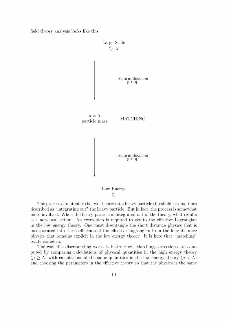
field theory analysis looks like this:

Large Scaleφj, χ

?

renormalizationgroup

µ = Λparticle mass MATCHING

?

renormalizationgroup

Low Energyφj

The process of matching the two theories at a heavy particle threshold is sometimesdescribed as “integrating out” the heavy particle. But in fact, the process is somewhatmore involved. When the heavy particle is integrated out of the theory, what resultsis a non-local action. An extra step is required to get to the effective Lagrangianin the low energy theory. One must disentangle the short distance physics that isincorporated into the coefficients of the effective Lagrangian from the long distancephysics that remains explicit in the low energy theory. It is here that “matching”really comes in.

The way this disentangling works is instructive. Matching corrections are com-puted by comparing calculations of physical quantities in the high energy theory(µ ≥ Λ) with calculations of the same quantities in the low energy theory (µ < Λ)and choosing the parameters in the effective theory so that the physics is the same

10

at the boundary (µ = Λ). Any interaction that is unchanged in the matching cancelsout of the matching because it contributes in the same way in the two theories. Thechange in a parameter in the effective theory due to matching is related, order byorder in perturbation theory, to a difference between the high energy and low energycalculations. In this difference, all effects of long distance physics, infrared diver-gences, physical cuts, etc., disappear, because they are the same, by construction,in the high and low energy theories. Thus only the short distance contributions areincorporated into the coefficients of the effective Lagrangian.

Heavy Quarks and the Velocity Superselection Rule

. . . strait is the gate, and narrow is the way, . . .

Mt. 7:14King James Version

The question is, what do you do if you are stuck at low energies (this often happensbecause of budgetary constraints — the taxpayers sometimes won’t build you a bigenough accelerator) but your universe contains a stable very heavy particle? Thisthings just lumbers along through your universe carrying a very large momentum.Because it’s momentum is huge, its evolution is essentially classical. What does theeffective field theory look like?

In the heavy quark example, the low energy scale I have in mind is ΛQCD, thetypical energy scale of the brown muck. A quark is heavy if mq À ΛQCD.

In these lectures, I will stick to the simple situation in which you have only oneheavy quark in your universe at any given time. If you have more than one, life getsmuch more difficult because the two heavy quarks can exchange gluons that carrylarge momenta.

However, we can imagine that the heavy quark changes its velocity in responseto some force that does not involve the QCD interactions. This does not pump anyenergy into the light quarks and gluons, so we stay at the energy scale of the brownmuck. Similarly, we can consider transitions between one heavy quark and another.No more energy is pumped into the brown muck when a b quark with velocity v iskicked by a weak current into a c quark with velocity v′, than when a c quark withvelocity v is kicked by an electromagnetic current into a c quark with velocity v′. Infact, as we have seen, the brown muck doesn’t know the difference.

The external currents are very useful as a way of keeping track of the trajectoryof the heavy quark. The external currents introduce kinks into the trajectories.

The question is, what does this effective theory look like? Evidently, the presenceof a heavy quark traveling with a definite velocity breaks Lorentz invariance, but wewould expect the invariance to be restored when we consider all possible heavy quarkvelocities. What is the symmetry structure of this peculiar theory?

Consider a heavy quark bound state with velocity v.

P µbound state = mbound statev

µ (2.23)

11

for large m,mquark ≈ mbound state

We expect the difference to be independent of mquark. We expect the heavy quark tocarry most, but not all of the momentum of the bound state. There will be a smallmomentum, qµ, of the brown muck from low energy QCD interactions. Then we canwrite

pµquark = P µ

bound state − qµ = mquarkvµ + kµ (2.24)

where this defines the small residual momentum

kµ = (mbound state −mquark)vµ − qµ

Now compare the 4-velocity fo the heavy quark with that of the state:

vµquark =

pµquark

mquark

= vµ + kµ/mquark (2.25)

They are the same in the heavy quark limit.

vµquark → vµ as mquark →∞

The QCD interactions do not change heavy quark’s velocity, no matter what thebrown muck is doing!

This leads to the velocity superselection rule. [12] Under the influence of theQCD interactions in the low energy theory, the heavy quarks move in straight linetrajectories. This is just conservation of momentum. If QCD interactions, by as-sumption, can only change the momentum by a small momentum, the change in the4-velocity, v = p/m, due to the soft QCD interactions is negligible. All the kinks inthe trajectories must be caused by some external (non-QCD) agency, like a weak

or electromagnetic interaction. These are represented by c†v′cv type operators thatannihilate a heavy quark with velocity v and create a heavy quark with velocity v′.

I will discuss three related (indeed equivalent) ways of looking at the effectivetheory — first looking at the action in momentum space — next discussing Feynmangraphs and the form of the propagator — and finally showing what is happening to thequark fields in position space. The starting point is always the relation pµ = mvµ+kµ.

First consider the functional integral in momentum space (the space is shown in

12

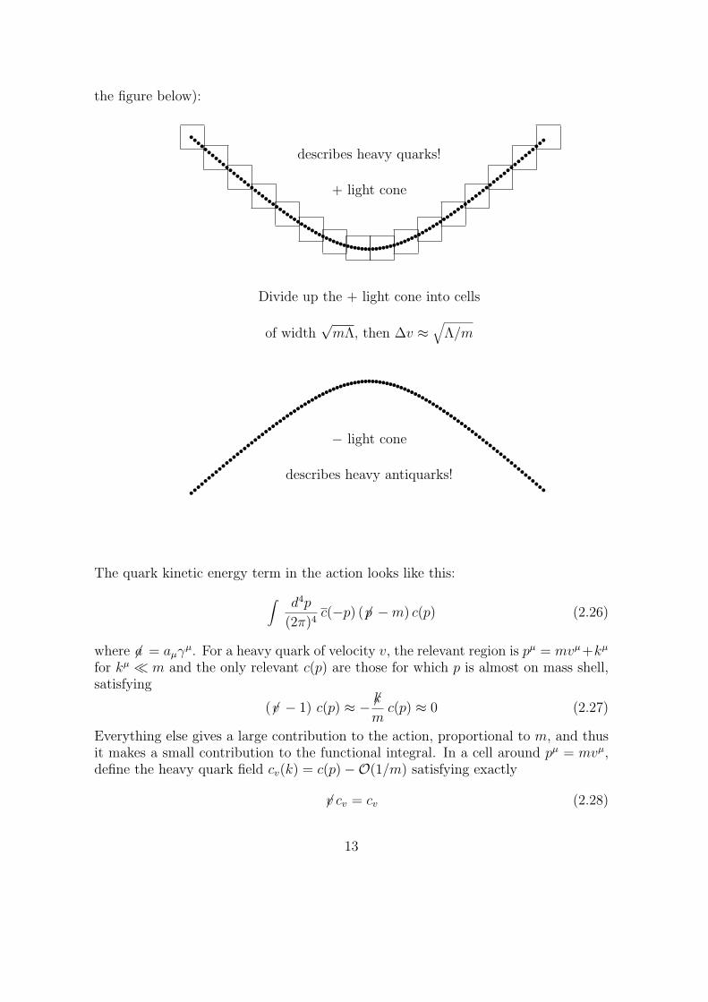
the figure below):

rrrrrrrrrrrrrrrrrrrrrrrrrrrrrrrrrrrrrrrrrrrrrrrrrrrrrrrrrrrrrrrrrrrr

rrrrrrrrr

rrrrrrrr

rrrrrrrr

rrrrrrr

rrrrrrrr

rrrrrrrr

rrrrrrrr

rrrrrrrrr

rrrrrrrrrrrrrrrrrrrrrrrrrrrrrrrrrrrrrrrrrrrrrrrrrrrrrrrrrrrrrrrrrrr

Divide up the + light cone into cells

of width√

mΛ, then ∆v ≈√

Λ/m

+ light cone

describes heavy quarks!

− light cone

describes heavy antiquarks!

The quark kinetic energy term in the action looks like this:

∫ d4p

(2π)4c(−p) ( 6p −m) c(p) (2.26)

where 6a = aµγµ. For a heavy quark of velocity v, the relevant region is pµ = mvµ+kµ

for kµ ¿ m and the only relevant c(p) are those for which p is almost on mass shell,satisfying

(6v − 1) c(p) ≈ − 6km

c(p) ≈ 0 (2.27)

Everything else gives a large contribution to the action, proportional to m, and thusit makes a small contribution to the functional integral. In a cell around pµ = mvµ,define the heavy quark field cv(k) = c(p)−O(1/m) satisfying exactly

6v cv = cv (2.28)

13

In other words, I am ignoring the variation of the spinor within the cell, because theeffect of this variation will vanish as m →∞.

Then in terms of the residual momentum, with k = p−mv small compared to m,the Lagrangian in the cell looks like

cv (6p −m) cv = cv 6k cv = cv vµkµ cv (2.29)

because

cv γµ cv =1

2cv {6v , γµ} cvcv vµ cv . (2.30)

Now as m →∞ and Λ →∞, the cells get closer together in velocity space, but thesize of each cell in momentum space also grows. Each cell becomes a mini-Lagrangianrelevant only for the heavy quark field with the corresponding velocity.

∫

cell

d4k

(2π)4cv(−k) vµkµ cv(k) . (2.31)

Next look at Feynman propagator in the full theory [13]

6p + m

p2 −m2 + iε(2.32)

If we insert pµ → mvµ + kµ and take the leading term in m in both the numeratorand the denominator

≈ m 6v + m

2m(vk) + iε=

1+ 6v2

1

(vk) + iε(2.33)

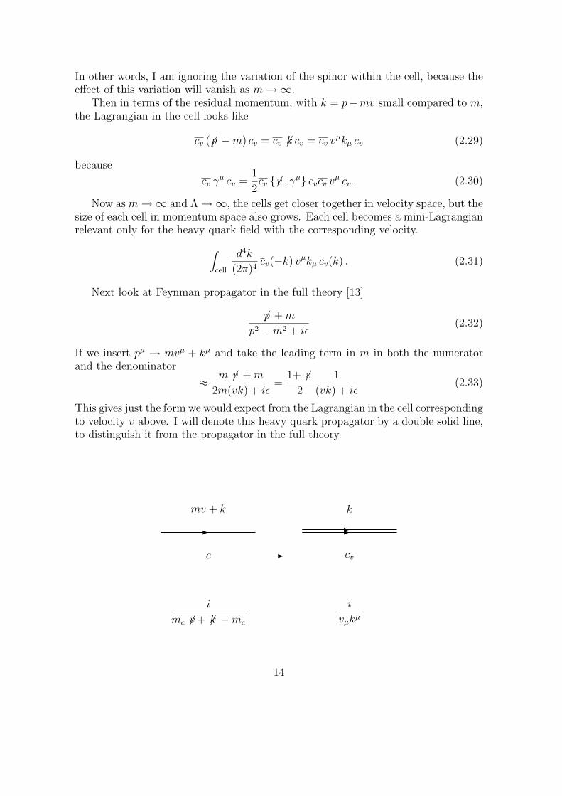
This gives just the form we would expect from the Lagrangian in the cell correspondingto velocity v above. I will denote this heavy quark propagator by a double solid line,to distinguish it from the propagator in the full theory.

- --

c cv

mv + k k

-

i

mc 6v + 6k −mc

i

vµkµ

14

Finally consider the Lagrangian in position space. In the full theory, the heavyquark field c has Lagrangian

L = c (i 6∂ −m) c (2.34)

— denote the heavy quark field by cv. The relation of cv with the usual heavy quarkfield c is the following (projecting away the negative light cone which corresponds tothe antiquarks):

c(x) =1+ 6v

2e−im vµxµ

cv(x) +O(1/m) (2.35)

L → icv vµ∂µ cv (2.36)

We have been ignoring the QCD interactions, but it is easy to incorporate them justby imposing the color gauge symmetry.

Lcv = i cv vµDµcv

This gives the same propagator again

1+ 6v2

1

(vk) + iε(2.37)

It is instructive to look at the propagator in position space. In the rest frame themomentum space propagator is

1 + γ0

2

1

k0 + iε(2.38)

The fourier transform is∝ δ3

(~r − ~r′

)Θ(t− t′) (2.39)

This just describes the particle sitting still, propagating in time along its classicaltrajectory.

The velocity superselection rule is equivalent to the statement that cv and cv′ areindependent fields for vµ 6= v′µ — they correspond to different cells on the massshell hyperboloid.

However, these unrelated independent fields are connected by Lorentz transfor-mations:

cv(x) → D(Λ)−1 cΛ−1v(Λ−1x) (2.40)

where D(Λ) = eiεµνσµνis the usual Dirac representation.

The Lagrangian is a sum (not an integral)3 over all v.

Lc =∑

~v

Lcv (2.41)

In this case, instead of integrating out heavy degrees of freedom, we have integratedextra degrees of freedom IN to describe the fact that infinitely heavy quarks with

3This is written down incorrectly in my original paper on heavy quark effective field theories.

15

different velocities have infinitely different momenta, and are therefore unrelated toeach other so far as the low energy theory is concerned.

Lcv = i cv vµDµcv

Heavy antiquarks, which I will denote by cv, can be treated in a similar way. Therelation of cv with the usual heavy quark field c is the following (this time projectingaway the quarks on the positive light cone):

cv(x) =1− 6v

2e−im vµxµ

c(x) (2.42)

L → −icv vµ∂µ cv (2.43)

Incorporating the color gauge symmetry gives the Lagrangian

Lcv = −i cv vµDµcv

Despite the −, this propagator is really almost the same as the quark propagator ifyou are describing heavy antiquarks propagating forward in time, because the creationand annihilation operators have been interchanged.4

In my original paper on the subject, I put the quark and antiquark Lagrangianstogether into a single structure using the Dirac algebra. While there is nothingreally wrong with this, it is potentially misleading, and I now think that it shouldbe avoided. In the low energy theory, the heavy antiquark has nothing to do withthe corresponding heavy quark (at least, in leading order in 1/m). They live in acompletely disconnected region of momentum space, infinitely far away in the heavyquark limit. The form of the Lagrangian should not disguise that fact.

We now will identify the symmetries of this system. It is simplest to see what thesymmetry looks like for a heavy quark in its rest system, v0 = 1, ~v = 0, for whichthe Lagrangian is

Lc0 = i c0 D0c0

whereγ0c0 = c0 (2.44)

This is invariant under rotation in the two dimensional space on which the heavyquark spinor is nonzero. To see what it looks like explicitly, we need a representationfor the γ matrices. It is simplest to take γ0 diagonal, so in a tensor product notation,

~σ ≡(

~σ 00 ~σ

), τ1 ≡

(0 II 0

), τ2 ≡

(0 −iIiI 0

), τ3 ≡

(I 00 −I

), (2.45)

we take γ0 = τ3, ~γ = i~στ1. Then the generators of the spin symmetry are

~S0 =(

1 + τ3

2

)~σ (2.46)

4As we will discuss below, the difference is only in the structure of the QCD interactions —antiquarks and quarks have different color charges.

16

Now look at the part of the Lagrangian describing a b quark at rest

Lb0 = i b0 D0b0

Lc0 + Lb0 has SU(4) symmetry. The reason is that the color interactions of the c0

and b0 are just the same. Both just produce a color Coulomb field in the rest frame.To see what the symmetry looks like, put the two field together into an 8-componentfield:

h0 ≡(

c0

b0

)(2.47)

thenLc0 + Lb0 = i h0 D0h0 (2.48)

In this 8 dimensional space, we need another set of Pauli matrices, ~η, that implementsthe SU(2) rotation between c and b subspaces. Then the Isgur-Wise SU(4) spin-flavorsymmetry is generated by

P0σj , P0ηj, , P0σjηk for j, k = 1 to 3 (2.49)

where

P0 =1 + τ3

2(2.50)

Let us now consider the general situation, for vµ

Lcv = i cv vµDµcv

Remember that because of the superselection rule, cv is a completely different fieldfrom c0.

We can define “spin” operators for any given vµ:

Svj = iεjk`[6e k, 6e `] (1+ 6v )/8 (2.51)

where eµj for j = 1 to 3 is an orthonormal set of space-like vectors orthogonal to vµ,

ejµeµk = −δjk , vµe

µj = 0 (2.52)

The Svj have the commutation relations of SU(2). Note that the S0

j could be definedin the same way with the ej

µ being unit vectors along the 1, 2 and 3 axes, ejµ = δµ

j .Now the Lagrangian is invariant under the transformation

δcv = i~ε · ~Sv cv (2.53)

It follows thatδcv = −i cv ~ε · ~Sv (2.54)

This looks more complicated than the v = 0 that we just discussed, but it really isn’t.In fact, we can go to the rest frame by a Lorentz transformation. This is the clue tothe symmetry structure of the heavy c quark Lagrangian.

17

There is one SU(2) for each v. Lorentz transformations change v, and with v, theSU(2)’s change as well. I’m not really sure what this symmetry structure is calledby mathematicians, but I will denote it by

SU(2)∞ ⊗ Lorentz

This is almost like a gauge symmetry, except that the Lorentz transformations alsorotate the SU(2)’s among themselves, because the eµ

j rotate under Lorentz transfor-mations.

The b quarks can be added in the same way as in the rest frame. The Lagrangianis

Lbv = i bv vµDµbv

and Lcv +Lbv has an SU(4) symmetry, constructed in the obvious way. If we put thec and b together as before,

hv ≡(

cv

bv

)(2.55)

then Isgur-Wise SU(4) spin-flavor symmetry is generated by

PvSvj , Pvηj, , PvS

vj ηk for j, k = 1 to 3 (2.56)

where

Pv =1+ 6v

2(2.57)

So the c-b system together has an

SU(4)∞ ⊗ Lorentz

symmetry structure.Note that the QCD interactions here are important. The heavy quark kinetic

energy (the sum over all v) has a much larger symmetry, because we can rotatequarks with different v’s into one another. But this symmetry is broken by theQCD interactions. For each v, there is a different characteristic color field producedby the heavy quark, just the Coulomb field in the appropriate rest frame.

Likewise, there is no symmetry between heavy quark and heavy antiquark, becausethe color interactions are different. On the over hand, heavy color triplets with otherspins (0, 1, etc.) could be included into the heavy quark formalism if Nature is sogenerous as to give such objects (relatively stable) to play with. The brown muckin a bound state of a heavy triplet scalar or gauge boson looks that same as in a Bmeson! [14, 15, 16]

18

Tensor Methods

Group theory is a useful technique, but it is no substitute for physics.

Lie Algebras in Particle PhysicsHoward Georgi

Sales of my group theory book have been dropping off lately — I thought that Ishould remind all of you that there is a lot of good pithy stuff there! I next want todevelop a tensor analysis to enable us to construct matrix elements consistent withthe SU(2)∞ ⊗ Lorentz symmetry in a simple and intuitive way. To do this, we willhave to find wave functions of heavy quark states in the effective theory consistentwith SU(2)∞ ⊗ Lorentz, and understand how to use them.

Tensor analysis is useful because it makes it easier both to calculate and to un-derstand the results of symmetry arguments.

A very familiar example is Gell-Mann’s SU(3). We could get all the informationabout the consequences of SU(3) symmetry just by clever use of raising and loweringoperators. But much easier to manipulate matrices, like

Σ0√2

+ Λ√6

Σ+ P+

Σ− −Σ0√2

+ Λ√6

N

Ξ− Ξ0 − 2Λ√3

(2.58)

The matrix, (2.58) is a generalized baryon wave function that includes flavor as anadditional index. It describes the wave functions of all the octet baryons at once. Thesymbols are labels for the different baryon wave functions. For example, to describea proton state, we would set P 6= 0 and all the other entries to 0.

Now lets look at the D and D∗ states and try to construct something similar. Wealready know the transformation properties of the fields under the SU(2)∞⊗Lorentzsymmetry. Let’s use them to construct the states. Define the wave functions asfollows:

D(v) ∝ 〈0| cvq |D, v〉

D(v, ε) ∝ 〈0| cvq |D∗, v, ε〉(2.59)

where ε is the D∗ polarization (ε∗µεµ = −1). D(v) and D(v, ε) are 4× 4 matrix wave

functions, analogous to a spinor wave function of a spin-12

fermion, F ,

uF (p) ∝ 〈0|ψ |F 〉 . (2.60)

The nice thing about this is that we know its symmetry properties. It has one indexthat transforms under the SU(2)v symmetry, the spin of the heavy quark, and it musttransform appropriately under Lorentz transformations.

19

Then the analog of the baryon matrix is the wave function of a general state

|D, v〉 ≡ d |D, v〉+∑ε

dε |D∗, v, ε〉 (2.61)

which isD(v) ∝ 〈0| cvq |D, v〉 = dD(v) +

∑ε

dε D(v, ε) (2.62)

Now d and dε are labels, like the baryon labels in (2.58), d = 1 in the D state anddε = 1 in D∗ state with polarization ε.

Because of the properties of cv, D(v) satisfies

6v D(v) = D(v) (2.63)

and transforms under SU(2)v as

D(v) → e−i~ε·~Sv

D(v) (2.64)

The set of all D(v) must also transform properly under Lorentz transformations:

D(v) → D(Λ)−1D(Λ−1v)D(Λ) (2.65)

The transformations (2.64) and (2.65) are the statement, in tensor language, of theSU(2)∞ ⊗ Lorentz symmetry. the SU(2)v spin symmetry that relates D and D∗ isnow automatically incorporated by using D instead of the separate wave functionsand constructing invariant matrix elements.

We can now use symmetry arguments to determine D(v) and D∗(v) almost com-pletely.

Lorentz invariance, parity and 6v D(v) = D(v) imply that we can take

D(v) = −√mD1+ 6v

2γ5 (2.66)

D(v, ε) =√

mD1+ 6v

26ε (2.67)

The overall normalization is completely arbitrary, however, we have the relativenormalization correct, up to a conventional phase between the D and D∗ states.We have included the factors of

√mD to make the counting of dimensions easier in

the applications that follow. Note that mD = mD∗ in the m → ∞ limit, so thedimensional factor is the mass of the state in both (2.66) and (2.67).

To see that the relative normalization is correct, let us look at the norms of thestates. These must satisfy (suppressing the momentum δ-function)

〈D, v |D, v〉 = 〈D∗, v, ε |D∗, v, ε〉

〈D∗, v, ε |D, v〉 = 〈D, v |D∗, v, ε〉 = 0

(2.68)

20

or〈D, v |D, v〉 ∝ |d|2 +

∑ε

|dε|2 (2.69)

As a first example of the use of tensor methods, let us check that (2.68) and(2.69) actually work. To do this, we have to introduce a little more formalism. Thematrix element is proportional to the wave functions put together consistent withthe SU(2)∞ ⊗ Lorentz symmetry. We already know that the |D, v〉 state has wavefunction D(v). The 〈D, v| state has a wave function proportional to D(v)∗, but thistransforms unpleasantly under SU(2)∞⊗Lorentz. We are familiar with this difficultyin dealing with fermion wave functions, u(p), where u(p)∗ transforms inconveniently,and instead we define a u(p) = u(p)†γ0 that is easier to handle. We can do the samething with the D(v)∗’s. They are, from (2.62),

D(v)∗ ∝ 〈D, v| (cvq)∗ |0〉 (2.70)

To turn the c∗v into cv and (q)∗ into q, we must transpose the matrix and multiply onboth sides by γ0. Thus it makes sense to define

D(v) ≡ γ0D(v)†γ0 ∝ 〈D, v| qcv |0〉 (2.71)

This object is acted on on the right by SU(2)v,

D(v) → D(v) ei~ε·~Sv

(2.72)

and it transform normally under the Lorentz symmetry,

D(v) → D(Λ)−1D(Λ−1v)D(Λ) (2.73)

We can now compute D(v) from D(v) and D(v, ε),

D(v) ≡ d∗ D(v) +∑ε

d∗ε D(v, ε) (2.74)

where because γ0㵆γ0 = γµ and γ0γ5†γ0 = −γ5,

D(v) =√

mD γ51+ 6v

2(2.75)

D(v, ε) =√

mD ε∗µγµ 1+ 6v

2(2.76)

We can now state the rule for computing matrix elements in the low energy theory

〈D′, v′| O |D, v〉 (2.77)

1. Replace the ket |D, v〉 by the wave function D(v);

2. Replace the bra 〈D, v| by the wave function D(v);

21

3. Put the wave functions together consistent with the SU(2)∞⊗Lorentz symmetryinto an object with the same symmetry structure as O. Each independent wayof putting things together gets multiplied by an unknown function of all theinvariants. Each of these functions must be fixed by the dynamics (or someother argument) in order to completely determine the matrix element.

Example 1 — we can now check (2.69): The heavy quark spin indices must becontracted for SU(2)v invariance. Then we must form a trace over the remainingDirac indices with all the possible Lorentz invariant combinations, 1, 6 v , 6 v 6 v , etc..Because D(v) 6v = −D(v) and 6v 6v = vµv

µ = 1, only the 1 term is independent. Wecan then explicitly work out the traces,

〈D, v |D, v〉 = tr(D(v)D(v)[A +

notindependent︷ ︸︸ ︷

B 6v + · · ·])

(2.78)

tr(D(v)D(v)

)= tr

(D(v, ε)D(v, ε)

)= −2mD (2.79)

tr(D(v, ε)D(v)

)= tr

(D(v)D(v, ε)

)= 0 (2.80)

For example, in detail, we have

tr(D(v, ε)D(v, ε)

)

= tr

(√mD ε∗µγ

µ 1+ 6v2

√mD

1+ 6v2

6ε)

= mD tr

(ε∗µγ

µ 1+ 6v2

6ε)

=1

2mD tr

(ε∗µγ

µ 6ε)

= −2mD

(2.81)

Thus

tr(D(v)D(v)

)= −2mD

(|d|2 +

∑ε

|dε|2)

(2.82)

and the result is

−2mDA

(|d|2 +

∑ε

|dε|2)

(2.83)

This means that (2.69) works and we got the relative normalization right.Example 2 — next consider the matrix element of the light quark vector current,

〈D, v| qγµq |D, v〉 = tr(D(v)D(v)[Avµ +

notindependent︷ ︸︸ ︷

B γµ + · · ·])

= −2AmDvµ

(|d|2 +

∑ε

|dε|2) (2.84)

22

Just as in example 1, we contract the heavy quark indices. Then put into the traceeverything that looks like a Lorentz vector. But all of these just reduce to vµ becauseof D(v) 6v = −D(v).

Here we know the answer!How? What is A?AnswerBecause qγµq is a conserved current, its forward matrix element is determined by

the charge, which here is −1 because the state contains one light antiquark

〈D, v| qγµq |D, v〉

= −2pµ

(|d|2 +

∑ε

|dε|2)

= −2mDvµ

(|d|2 +

∑ε

|dε|2)

(2.85)

A = 1

Thus the result of the spin symmetry in this case is nothing that we do not alreadyknow. However, for qDµq, for example, the spin symmetry argument would be exactlythe same, and gives the same matrix elements up to a constant. Thus for the currentqDµq, the relation between the D and D∗ states is a nontrivial consequence of theSU(2)∞ ⊗ Lorentz symmetry.Example 3 — let’s work out the matrix element of an axial vector current. Onceagain, there is only one invariant, which looks like this (note that vµγ5 vanishesbecause of D(v) 6v = −D(v)):

〈D, v| qγµγ5q |D, v〉 = tr(D(v)D(v)[Aγµγ5]

)

= −2AmD

∑ε (d∗εdεµ∗ + d∗dεε

µ)

(2.86)

From this we extract.

〈D∗(v, ε)| qγµγ5q |D(v)〉 = −2AmDεµ∗ (2.87)

〈D(v)| qγµγ5q |D∗(v, ε)〉 = −2AmDεµ (2.88)

This result is not interesting because the answer couldn’t have been anything else,but there is a moral hidden in the computation. The γµγ5 appears in the trace,not just because it’s in the current — it is simply the most general thing consistentwith Lorentz invariance and Parity and D(v) 6 v = −D(v)! In fact, the argument isprecisely the same for a current like i q Dµγ5 q.

Now for a trick question. What is

〈D′, v′| qq |D, v〉 (2.89)

23

for v′ 6= v?The answer is 0! In the low energy theory, by definition, QCD interactions can’t

change heavy quark velocities. This is forbidden by the velocity superselection rule.Such a change in velocities would require a large, O(mc), transfer of energy from thebrown muck to the heavy quarks, which would take us out of the effective theory.

Now for a more serious question, indeed, related to the central question of theselectures. What is

〈D′, v′| cv′Γcv |D, v〉 (2.90)

where Γ is some 4× 4 matrix like γµ or σµνγ5 (only 2× 2 really counts — because of6v D(v) = D(v) and D(v, ) 6v ′ = D(v′) the space is really 2× 2)?

There are two equivalent ways of thinking of thinking about this matrix element.We can figure out how cv′Γcv transforms for some fixed Γ and follow the rules, or whatis more convenient, we can extend the rules to incorporate the notion of “tensoroperators”. This goes as follows. If Γ were a field transforming as

Γ → e−i~ε′·~Sv′Γei~ε·~Sv

(2.91)

then the operator would be invariant under the spin symmetries. A field Γ trans-forming this way is a tensor. It is a kind of wave function for the current operator.If we imagine that we are computing the matrix element of the current multiplied bythis tensor field, Γ, we can impose the spin symmetry by simply requiring invarianceunder all of the relevant SU(2)v’s. Then at the end of the day, we can set Γ equal towhatever constant value we are interested in, and we will have the right symmetrystructure.

This leads to an improved rule for computing matrix elements in low energy theory

〈D′, v′| O |D, v〉 (2.92)

1. Replace the |D, v〉 by the wave function D(v).

2. Replace the 〈D′, v′| by the wave function D′(v′)

3. Replace the operators by tensors transforming appropriately under SU(2)∞.

4. Put the wave functions together into invariants under SU(2)∞, transformingappropriately under Lorentz transformations. Still, for each independent in-variant, we must include an arbitrary function of the Lorentz invariants. Eachof these must be fixed by the dynamics (or some other argument).

Let’s do it! The argumentation should now be familiar. We just have to contract

both sets of spin indices to make an invariant both under SU(2)v and SU(2)v′ . Asbefore there is only one term. This time, we have more objects that can contribute,because there are two vectors, v and v′, but when we impose D(v) 6 v = −D(v) and

24

6v ′D(v′) = −D(v′), they all reduce to a single unknown function of the invariant, v′v.

〈D, v′| cv′Γcv |D, v〉

= tr(D(v′)ΓD(v)[−ξ(v′v) +

notindependent︷ ︸︸ ︷

χ(v′v) 6v + · · ·])

= −ξ(v′v) tr(D(v′)ΓD(v)

)

(2.93)

If we choose the normalization right, this ξ(v′v) is the Isgur-Wise function that wediscussed in the first lecture. As we will show shortly, the last line of (2.93) producesthe right normalization (that is why we included the minus sign, as well as callingthe coefficient ξ(v′v) with no extra factors).

We can get the normalization information by looking at the forward matrix ele-ment of Γ = γµ, the vector current:

〈D, v′| cv′γµcv |D, v〉

= −ξ(v′v) tr(D(v′)γµD(v)

) (2.94)

We must simply insert into (2.93) the expressions for D(v) and D(v′),

D(v) =√

mD1+ 6v

2

(−dγ5 +

∑ε

dε 6ε)

(2.95)

D′(v′) =√

mD

(d′∗γ5 +

∑

ε′d′∗ε′ε

′∗µγ

µ

)1+ 6v ′

2(2.96)

This gives a complicated but interesting expression that we will compute in a momentin the context of b → c transitions. But at v′ = v it is simple

= ξ(1) 2mDvµ

d′∗d−∑

ε′,εd′∗ε′dε(ε

′∗µε

µ)

(2.97)

But now we know that ξ(1) = 1 because

cvγµcv = vµ cvcv (2.98)

is the symmetry current that counts the heavy cv quarks. Thus (2.93) is correct forthe conventionally normalized Igsur-Wise function that is 1 at the Shifman-Voloshinpoint, v′v = 1.

Phenomenologically more interesting are the cv′Γbv currents. The analysis of theirmatrix elements in the effective low energy theory is entirely analogous to the dis-cussion above. Just make the replacements c → b, D → B and D → B. This works

25

because in the theory with both a heavy b and a heavy c (which we are in when we arebelow the scale mc) there is actually an SU(4)∞ ⊗ Lorentz symmetry that behavesin exactly the same way as the SU(2)∞ ⊗ Lorentz symmetry that we used above. Ifwe wanted to, we could write all the wave functions in a 8 dimensional space, but thesymmetry that rotates the b into the c is so trivial that it hardly warrants this ex-cessively formal notation. We will simply remember that we could do it if we wantedto. The result for the transition matrix element looks exactly like (2.93)

〈D′, v′| cv′Γbv |B, v〉

= ξ(v′v)√

mDmB tr

[(d′∗γ5 +

∑

ε′d′∗ε′ε

′∗µγ

µ

)

· 1+ 6v ′2

Γ1+ 6v

2

(−bγ5 +

∑ε

bε 6ε)]

(2.99)

For example, we can extract the matrix elements for Γ = γµ and Γ = γµγ5 that arerelevant to the dominant semileptonic weak decays of the B.

In the low energy theory, it is exactly the same Isgur-Wise function that comes into(2.99) and (2.93). This, at low energies, depends only on the brown muck. Formally,in the effective low energy theory, this is a consequence of the SU(4)∞ ⊗ Lorentzsymmetry.

Working out the relevant matrix elements explicitly, we find

〈D, v′| cv′γµbv

∣∣∣B, v⟩

= ξ(v′v)√

mDmB tr

(γ5

1+ 6v ′2

γµ 1+ 6v2

γ5

)

= ξ(v′v)√

mDmB

(vµ + v′µ

)(2.100)

〈D∗, ε′, v′| cv′γµbv

∣∣∣B, v⟩

= ξ(v′v)√

mDmB tr

(ε′∗νγ

ν 1+ 6v ′2

γµ 1+ 6v2

γ5

)

= ξ(v′v)√

mDmBε′∗ν4

tr (γν 6v ′γµ 6v γ5)

= iξ(v′v)√

mDmB εµναβ ε′∗νvαv′β

(2.101)

becausetr

(γµγνγαγβγ5

)= i εµναβ (2.102)

26

and

〈D∗, ε′, v′| cv′γµγ5bv

∣∣∣B, v⟩

= ξ(v′v)√

mDmB tr

(ε′∗νγ

ν 1+ 6v ′2

γµγ51+ 6v

2γ5

)

= ξ(v′v)√

mDmB tr

(ε′∗νγ

ν 1+ 6v ′2

γµ 1− 6v2

)

= ξ(v′v)√

mDmB

[(1 + v′v) ε′µ∗ − ε′ν∗vνv

′µ]

(2.103)

Matching and Running

My object all sublimeI shall achieve in time —To make the punishment fit the crime —The punishment fit the crime

The MikadoGilbert and Sullivan

So far, we have been at low energies — kµ, µ ¿ mb, mc. To complete the calculation ofmatrix elements between heavy meson states, we must answer the following question.How are operators in the low energy theory related to currents in the full theory? Inparticular, consider the relation between cΓb and cv′Γbv.

The effective field theory formalism gives us a crank to turn to find this relation,shown in the figure below.

We begin at high energies, where we know the form of the semileptonic weakinteractions in terms of the currents in the full QCD theory. We start by matchingthe physics in two theories on either side of the scale µ = mb

High energies ↓normal quarks

µ = mb match physics

b heavy ↓RG running

c normal ↓

µ = mc match physics

both heavy ↓

µ ≈ Λ compute m.e.

27

There are two approximations involved — 1/mb and αs(mb).In leading order in both αs and 1/mb, the matching is trivial:

b(x) → e−imb vµxµ

bv(x) (3.104)

cΓb → e−imb vµxµ

cΓbv

In momentum space, the e−imb vµxµsimply eliminates all effects of order mb, as shown

diagrammatically below:

t t

µ > mb µ < mb

b c cbv

©©©*©©©©©HHHj

HHHHH

Γ Γ

mbvµ + kµ pµ

©©©*©©©*©©©©©

©©©©©HHHjHHHHH

kµ pµ→

For µ > mb, cΓb doesn’t depend on µ (because it is the Noether current associatedwith a softly broken symmetry), but in low energy theory, mc < µ < mb, there is nosymmetry. Thus we expect that the current has a nonzero anomalous dimension. Tocompute it, we need three Feynman graphs

Γ

¡¡

¡¡

¡¡

¡¡

¡¡

¡¡

¡¡

¡¡

¡¡

¡¡

¡¡¡µ

¡¡¡µ

¡¡¡µ

¡¡¡µ

t@

@@

@@

@@

@@

@

@@@R

@@@R

©©©©©©©©©©®®®®®®®®®®£¢ £¢ £¢ £¢ £¢ £¢ £¢ £¢ £¢ £¢

bv c

← qk p

k + q p + q

and the self energies of the bv and c

-- --©©©©©©©©©©®®®®®®®®®®£¢ £¢ £¢ £¢ £¢ £¢ £¢ £¢ £¢ £¢

' $' $--

bv bv

k ← q

k + q

k

28

and

- -

-

©©©©©©©©©©®®®®®®®®®®£¢ £¢ £¢ £¢ £¢ £¢ £¢ £¢ £¢ £¢

' $-

c c

p ← q

p + q

p

We will compute them in reverse order, using dimensional regularization (DR) andminimal subtraction (we’ll only worry about anomalous dimensions to one loop, sothere is no difference between MS and MS).

The tools we need will be the standard ones. Combining denominators, with theFeynman trick, and extending the theory to n = 4− ε dimensions, for regularization,where the typical Feynman integral looks like

∫ dn`

(2π)n

(`2)β

(`2 − A2)α

=i

(4π)n/2(−1)α+β(A2)β−α+n/2

·Γ(β + n/2) Γ(α− β − n/2)

Γ(n/2)Γ(α)

(3.105)

The issue of infrared (IR) divergences in dimensional regularization is sometimesconfusing, so I will begin with a digression.

The physical idea of a regularization scheme is that it is a modification of thephysics of the theory at short distances that allows us to calculate the quantumcorrections. If we modify the physics only at short distances, we expect that all theeffects of the regularization can be absorbed into the parameters of the theory. Thatis how we chose the parameters in the first place. However, it is not obvious thatDR is a modification of the physics at short distances. To see to what extent it is,consider a typical Feynman graph in the unregularized theory in Euclidean space.In one loop (which I discuss for simplicity), all graphs ultimately reduce to sums ofobjects of the following form:

I =∫

[dx]d4`

(2π)4

1

(`2 + A2)α, (3.106)

α is some integerIn DR, these get replaced by integrals over 4 + δ dimensional momentum space. I

am going to think of ε = −δ as being negative. This doesn’t really matter, because

29

everything is defined by analytic continuation anyway, but it makes things easier totalk about. The regularized integrals have the form

Iδ = c(δ)∫

[dx]d4+δ`

µδ (2π)4+δ

1

(`2δ + `2 + A2)α

, (3.107)

where c(δ) → 1 as δ → 0, and where I have explicitly separated out the “extra” δdimensions, so that `2 is the 4 dimensional length.

In practice, we would do the whole n dimensional integral at once, using (3.105).However, to see what is happening, I am going to split the integral up into an integralover the usual 4 dimensions and the extra δ dimensions. Rewrite the integral asfollows:

c(δ)∫

[dx]dδ`

(2πµ)δ

d4`

(2π)4

1

(`2δ + `2 + A2)α

, (3.108)

Now do integral over δ extra dimensions

Iδ =∫

[dx]d4`

(2π)4

1

(`2 + A2)αr(δ)

(`2 + A2

4πµ2

)δ/2

, (3.109)

where

r(δ) = c(δ)Γ(α− δ/2)

Γ(α). (3.110)

The factor r(δ) → 1 as δ → 0. The important factor is

ρδ/2 where ρ =`2 + A2

4πµ2. (3.111)

This also → 1 as δ → 0, but here convergence depends on ` and A.

ρδ/2 = e(δ ln ρ)/2 , (3.112)

ρδ/2 ≈ 1 for | ln ρ| ¿ 1

δ. (3.113)

You can see from (3.113), that for very small δ, we have not changed the physicsfor ` (the loop momentum) and A (which involves external momenta and masses)of the order of µ, but that there are significant differences if either ` or A is muchlarger than µ for fixed δ, or if they are both much smaller than µ. The first isexactly what we want. This is just a modification of the physics at short distances.The second is the problem. DR can modify the physics at large distances as well, sothat, in general, it is not a sensible regulator.

However, we are OK so long as we avoid IR divergences. Then small momentadon’t contribute in the integrals (A cannot get very small). We can always do this inthe calculation of an anomalous dimension or a matching contribution. In matching,it is trivial. The matching is chosen so that the infrared physics is exactly the same in

30

the two effective theories, so that the IR divergences always cancel in the calculation.In calculating an anomalous dimension, the IR region is also irrelevant. For example,we can keep external momenta nonzero until after renormalization, eliminating IRdivergences. However, we will do this in out heads, because the final result for theanomalous dimension doesn’t depend on the external momentum.

First consider the light quark self energy:

- -

-

©©©©©©©©©©®®®®®®®®®®£¢ £¢ £¢ £¢ £¢ £¢ £¢ £¢ £¢ £¢

' $-

c c

p ← q

p + q

p

In Feynman gauge and n = 4− ε dimensions, the corresponding Feynman integral is

∫ dnq

(2π)n

−i

q2 + iε[(−igµε/2)T aγν i(6q + 6p )

(q + p)2 + iε(−igµε/2)T aγν

] (3.114)

= −4

3g2µε

∫ dnq

(2π)n

γν(6q + 6p )γν

(q + p)2q2(3.115)

I’ve dropped iεWe are only interested in the 1/ε and ln µ terms, so we can do Dirac manipulations

for ε = 0, to get

=8

3g2µε

∫ dnq

(2π)n

(6q + 6p )

(q + p)2q2(3.116)

Then combining denominators using the Feynman trick gives

1

(q + p)2q2=

∫ 1

0dx

1

[q2 + 2xpq + xp2]2(3.117)

and q → `− xp

=8

3g2µε

∫ dn`

(2π)n

∫ 1

0dx

(6` + (1− x)6p )

[`2 + x(1− x)p2]2(3.118)

=4

3g2µε 6p

∫ dn`

(2π)n

1

[`2]2(3.119)

31

where I finally dropped the external momentum dependence, which was interestingonly because it was acting as an IR cutoff. The using (3.107), and Γ(ε) = 1

ε+ · · · we

get the final result for the 1/ε term,

8

3

g2

16π2

µε

εi 6p (3.120)

Then after the 1/ε pole is removed by MS, the two point function is

Γc2 = i 6p

(1 +

8

3

g2

16π2ln µ + · · ·

)(3.121)

From this we can calculate the anomalous dimension by requiring that RGE be sat-isfied (

µ∂

∂µ+ β(g)

∂

∂g+ 2γc

)Γc

2 = 0 (3.122)

The β function is β(g) = O(g3) and so irrelevant, thus

γc = −4

3

g2

16π2(3.123)

This should be familiar.Now let’s do the same thing for self energy of the bv:

-- --©©©©©©©©©©®®®®®®®®®®£¢ £¢ £¢ £¢ £¢ £¢ £¢ £¢ £¢ £¢

' $' $--

bv bv

k ← q

k + q

k

∫ dnq

(2π)n

−i

q2 + iε[(−igµε/2)T avν i

qv + kv + iε(−igµε/2)T avν

]

= −4

3g2

∫ dnq

(2π)n

1

(q2)(qv + kv)

(3.124)

I expect a result proportional to (kv), the tree term in the 2-point function. To isolateit, expand in (kv), keep the linear term, then set k = 0 (except for its job as an IRregulator):

=4

3g2µε (kv)

∫ dnq

(2π)n

1

(q2)(qv)2(3.125)

32

There are lots of ways of doing these funny looking Feynman integrals. I am goingto show you a method that, I think, always works, at least for finding anomalousdimensions. After you have combined the normal Feynman propagators, combinethem with the funny looking denominators using the following identity:

1

(q2)n(qv)m=

(n + m− 1)!

(n− 1)! (m− 1)!

∫ ∞

0

2mλm−1dλ

(q2 + 2λqv)n+m(3.126)

Here, this gives

=32

3g2µε (kv)

∫ dnq

(2π)n

∫ ∞

0

λ dλ

(q2 + 2λqv)3(3.127)

Next shift to eliminate linear terms in q, q = `− λv

=16

3g2µε (kv)

∫ dn`

(2π)n

∫ ∞

0

dλ2

(`2 − λ2)3(3.128)

Now rescale to a dimensionless integration variable, κ, pulling out a factor of√−`2

(`2 < 0 because we are in Euclidean space in our Feynman integrals)

λ2 = −`2 κ2 (3.129)

which gives

= −16

3g2µε (kv)

∫ dn`

(2π)n

1

(`2)2·∫ ∞

0

dκ2

(1 + κ2)3(3.130)

This breaks the integral up into two pieces, one of which is the normal log divergent(in n = 4) part, and the other of which is a convergent integral over κ.

Doing the κ integral is trivial, and gives

= −8

3g2µε (kv)

∫ dn`

(2π)n

1

(`2)2(3.131)

= −16

3

g2

16π2

µε

εi(kv) + · · · (3.132)

Then after renormalization, the two point function is

Γbv2 = i(kv)

(1− 16

3

g2

16π2ln µ + · · ·

)(3.133)

and using the RGE as before leads to

γbv =8

3

g2

16π2(3.134)

33

Finally. look at the three point function.

Γt

¡¡

¡¡

¡¡

¡¡

¡¡

¡¡

¡¡

¡¡

¡¡

¡¡

¡¡¡µ

¡¡¡µ

¡¡¡µ

¡¡¡µ

@@

@@

@@

@@

@@

@@@R

@@@R

©©©©©©©©©©®®®®®®®®®®£¢ £¢ £¢ £¢ £¢ £¢ £¢ £¢ £¢ £¢

bv c

← qk p

k + q p + q

Setting external momenta to zero, the Feynman integral is

∫ dnq

(2π)n

−i

q2[(−igµε/2)T aγν i 6q

q2Γ

i

qv(−igµε/2)T avν

]

= −i4

3g2µε 6v

∫ dnq

(2π)n

6q(q2)2(qv)

Γ

= −i16

3g2µε 6v

∫ dnq

(2π)n

∫ ∞

0dλ

6q(q2 + 2λqv)3

Γ

= −i16

3g2µε 6v

∫ dn`

(2π)n

∫ ∞

0dλ

6` − λ 6v(`2 − λ2)3

Γ

= i8

3g2µε Γ

∫ dn`

(2π)n

∫ ∞

0

dλ2

(`2 − λ2)3

(3.135)

This is the same integral as before, so the result for the vertex is

ΓcΓbv =

(1 +

8

3

g2

16π2ln µ + · · ·

)Γ (3.136)

This must satisfy the RGE

(µ

∂

∂µ+ β(g)

∂

∂g+ γc + γbv − γcΓbv

)ΓcΓbv = 0 (3.137)

or

γcΓbv = 4g2

16π2(3.138)

The β-function is

µ∂

∂µg ≡ β(g) = − b g3

16π2= −33− 2nq

3

g3

16π2= −25

3

g3

16π2(3.139)

34

where nq the number of light quarks, bv doesn’t count because we cannot producequark antiquark pairs in the effective low energy theory. If you explicitly computethe contribution of a bv loop to the gluon self energy, you get zero, as you expect. Inthe rest frame, in position space, this is particularly trivial — the heavy b0 quark canpropagate only forward in time, so there is no way to make a loop.

The running coupling isαs(µ)

4π≈ 1

2b ln µ/Λ(3.140)

Now the matrix element M(µ) = 〈D| cΓbv |B〉 depends on µ.(µ

∂

∂µ+ β(g)

∂

∂g− γcΓbv

)M(µ) = 0 (3.141)

The solution is

M(µ) = M(µ0) · exp

(∫ µ

µ0

γcΓbv(g(µ′))dµ′

µ′

)

= M(µ0) · exp

(∫ g(µ)

g(µ0)

γcΓbv(g′)

β(g′)dg′

)

≈ M(µ0) · exp(−12

25(ln g(µ)− ln g(µ0))

)

= M(µ0) ·(

αs(µ)

αs(µ0)

)− 625

(3.142)

M(mb) is related to the matrix element in the full theory

M(mb) = M(µ) ·(

αs(mb)

αs(µ)

)− 625

(3.143)

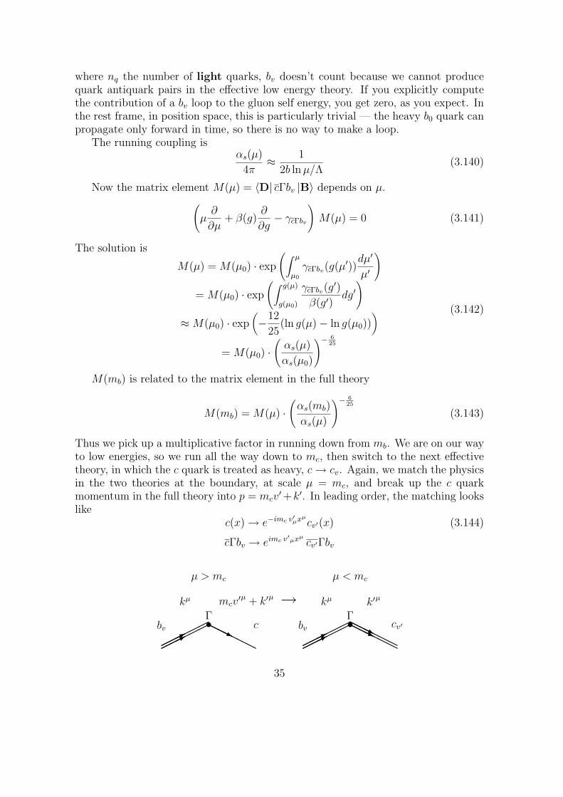
Thus we pick up a multiplicative factor in running down from mb. We are on our wayto low energies, so we run all the way down to mc, then switch to the next effectivetheory, in which the c quark is treated as heavy, c → cv. Again, we match the physicsin the two theories at the boundary, at scale µ = mc, and break up the c quarkmomentum in the full theory into p = mcv

′+k′. In leading order, the matching lookslike

c(x) → e−imc v′µxµ

cv′(x) (3.144)

cΓbv → eimc v′µxµ

cv′Γbv

t t

µ > mc µ < mc

bv c cv′bv

©©©*©©©*©©©©©

©©©©©HHHjHHHHH

Γ Γkµ mcv

′µ + k′µ

©©©*©©©*©©©©©

©©©©©HHHjHHHjHHHHH

HHHHH

kµ k′µ→

35

Now finally, we must do the most interesting anomalous dimension calculation,for the anomalous dimension of cv′Γbv.[17]

Γt

¡¡

¡¡

¡¡

¡¡

¡¡

¡¡

¡¡

¡¡

¡¡

¡¡

¡¡¡µ

¡¡¡µ

¡¡¡µ

¡¡¡µ

@@

@@

@@

@@

@@

@@@R

@@@R

@@

@@

@@

@@

@@

@@@R

@@@R

©©©©©©©©©©®®®®®®®®®®£¢ £¢ £¢ £¢ £¢ £¢ £¢ £¢ £¢ £¢

bv cv′

← qk k′

k + q k′ + q

Again setting external momenta to zero, the integral is

∫ dnq

(2π)n

−i

q2

[(−igµε/2)T av′ν

i

qv′Γ

i

qv(−igµε/2)T avν

]

= −i4

3g2µε v′v

∫ dnq

(2π)n

Γ

(q2)(qv)(qv′)

= −i32

3g2µε v′v ·

∫ dnq

(2π)n

∫ ∞

0dλ

∫ ∞

0dλ′

Γ

(q2 + 2λqv + 2λ′qv′)3

(3.145)

= −i32

3g2µε v′v ·

∫ dn`

(2π)n

∫ ∞

0dλ

∫ ∞

0dλ′

Γ[`2 − (λ2 + λ′2 + 2v′vλλ′)

]3 (3.146)

Now rescaleλ =

√−`2 κ , λ′ =

√−`2 κ′ (3.147)

giving

= i32

3g2µε v′v

∫ dn`

(2π)n

1

(`2)2·∫ ∞

0dκ

∫ ∞

0dκ′

Γ(1 + κ2 + κ′2 + 2v′vκκ′

)3 (3.148)

Now we can do the dn` integral

= −64

3

g2

16π2

µε

εv′v ·

∫ ∞

0dκ

∫ ∞

0dκ′

Γ(1 + κ2 + κ′2 + 2v′vκκ′

)3

= −32

3

g2

16π2

µε

εv′v ·

∫ ∞

0dκ2

∫ π/2

0dθ

Γ

[1 + κ2(1 + v′v sin 2θ)]3

= −16

3

g2

16π2

µε

εv′v Γ ·

∫ π/2

0

dθ

(1 + v′v sin 2θ)

= −16

3

g2

16π2

µε

εv′v r(v′v) Γ

(3.149)

36

where

r(w) =ln

(w +

√w2 − 1

)

√w2 − 1

(3.150)

The θ integral is best done by a symbolic manipulation program, however, if youhunker down to it, it is not so hard.

∫ π/2

0

dθ

(1 + w sin 2θ)(3.151)

let z = e2iθ, integral can be deformed to real axis

=∫ −1

1

dz

2iz

1(1 + w

2i[z − z−1]

)

=∫ −1

1

dz

w

1

(z2 + 2iz/w − 1)

=∫ −1

1

dz

w

1(z + i

w−

√w2−1w

) (z + i

w+

√w2−1w

)

=1

2√

w2 − 1

∫ −1

1

1(

z + iw−

√w2−1w

) − 1(z + i

w+

√w2−1w

)

=1

2√

w2 − 1ln

(−1 + i

w−

√w2−1w

)(1 + i

w−

√w2−1w

)(1 + i

w+

√w2−1w

)(−1 + i

w+

√w2−1w

)

(3.152)

=1

2√

w2 − 1ln

((w +

√w2 − 1)2 + 1

(w −√w2 − 1)2 + 1

)

=1

2√

w2 − 1ln

(w +

√w2 − 1

w −√w2 − 1

)

=1√

w2 − 1ln

(w +

√w2 − 1

)

(3.153)

Thus finally, the 3-point function is

Γcv′Γbv =

(1− 16

3

g2

16π2(v′v r(v′v)) ln µ + · · ·

)Γ (3.154)

This must satisfy the RGE(µ

∂

∂µ+ β(g)

∂

∂g+ γc′v + γbv − γcv′Γbv

)Γcv′Γbv = 0 (3.155)

or

γcv′Γbv = −16

3

g2

16π2(v′v r(v′v)− 1) (3.156)

37

Note that anomalous dimension vanishes for v′v = 1, symmetry current, which weknow on general grounds does not run.

Now solving the RGE and putting this together with the previous calculation, wehave the final result for the relation between the current in the full theory and thelow energy effective theory in leading order in 1/m and αs

q′Γq = Cq′q(µ) q′v′Γqv (3.157)

where for mq′ < mq

Cq′q(µ) =

(αs(mq)

αs(mq′)

)− 633−2nq

(αs(mq′)

αs(µ)

) 8(v′v r(v′v)−1)33−2nq

(3.158)

While we cannot compute the low energy matrix element, we expect it to givenapproximately by dimensional analysis if we take µ ≈ ΛQCD, so that the importantmultiplicative factor is

Cq′q = Cq′q(Λ) (3.159)

This gives the final result:

〈D, v′| cγµµb∣∣∣B, v

⟩

= Ccb ξ(v′v)√

mDmB

(vµ + v′µ

) (3.160)

〈D∗, ε′, v′| cγµb∣∣∣B, v

⟩

= iCcb ξ(v′v)√

mDmB εµναβ ε′∗νvαv′β

(3.161)

〈D∗, ε′, v′| cγµγ5b∣∣∣B, v

⟩

= Ccb ξ(v′v)√

mDmB

[(1 + v′v) ε′µ∗ − ε′ν∗vνv

′µ] (3.162)

〈D, v′| cγµµb∣∣∣D, v

⟩

= Ccc ξ(v′v) mD

(vµ + v′µ

) (3.163)

〈D∗, ε′, v′| cγµb∣∣∣D, v

⟩

= iCcc ξ(v′v) mD εµναβ ε′∗νvαv′β

(3.164)

〈D∗, ε′, v′| cγµγ5b∣∣∣D, v

⟩

= Ccc ξ(v′v) mD

[(1 + v′v) ε′µ∗ − ε′ν∗vνv

′µ] (3.165)

38

This is the fundamental result of the heavy quark effective field theory. You cannow try to improve on this by incorporating higher order effects in αs and 1/m. Theαs corrections are straightforward applications of QCD perturbation theory in thetwo theories. The 1/m terms, on the other hand, involve new, higher dimensionoperators, who matrix elements are new nonperturbative functions. This generallyintroduces much additional uncertainty into the game, except at the Shifman-Voloshinpoint [18, 19], or the spin 1/2. Λc and Λb baryons [20], where things are still relativelysimple.

AcknowledgementsI am grateful to Mark Wise for sending me reference [21] before publication. This

work was supported in part by the National Science Foundation under Grant #PHY-8714654; and by the Texas National Research Laboratory Commission, under Grant#RGFY9106. Harvard preprint #HUTP-91/A039.

References

[1] N. Isgur and M. B. Wise, Phys. Lett. 232B (1989) 113; 208B (1988) 504.

[2] E. Eichten and B. Hill, Phys. Lett. 234B (1990) 511.

[3] T. Appelquist and H. D. Politzer, Phys. Rev. Letters 34 (1975) 43.

[4] H. Georgi, Weak Interactions and Modern Particle Theory Ben-jamin/Cummings, Menlo Park, CA, 1984.

[5] A. De Rujula et al., Phys. Rev. D12 (1975) 147.

[6] S. Nussinov and W. Wetzel, Phys. Rev. D36 (1987) 130.

[7] M. Suzuki, Nucl. Phys. B258 (1985) 553; B. Grinstein, M. B. Wise and N. Isgur,Phys. Rev. Lett. 56 (1986) 286; T. Altomari and L. Wolfenstein, Phys Rev. Lett58 (1987) 1583; N. Isgur, D. Scora, B. Grinstein and M. B. Wise, Phys. Rev.D39 (1989) 799.

[8] E. Eichten and F. L. Feinberg, Phys. Rev. Lett. 43 (1979) 1205; Phys. Rev. D23(1981) 2724; E. Eichten in Field Theory on the Lattice, Proc. Intern. Symp.(Seillac, France, 1987) ed. by A. Billoire et al.,Nucl. Phys. B (Proc. Suppl.) 4(1988) 170.

[9] G. P. Lepage and B. A. Thacker, Cornell Report No. CLNS 87/114 (1987), in:Field Theory on the Lattice, Proc. Intern. Symp. (Seillac, France, 1987), ed.A. Billoire et al.,Nucl. Phys. B (Proc. Suppl.) 4 (1988) 199; W. E. Caswell andG. P. Lepage, Phys. Lett. 167B (1986) 437.

39

[10] M. B. Voloshin and M. A. Shifman, Yad. Fiz. 45 (1987) 463 [Sov. J. Nucl. Phys.45 (1987) 292], and Sov. J. Nucl. Phys. 47 (1988) 511.

[11] H. D. Politzer and M. B. Wise, Phys. Lett. 206B (1988) 681; 208B (1988) 504.

[12] H. Georgi, Phys. Lett. 240B (1990) 447. See also J. D. Bjorken, SLAC-PUB-5278, invited talk at Recontre de Physique de al Vallee d’Acoste, La Thuile, Italy(1990) unpublished.

[13] B. Grinstein, Nucl. Phys. B339 (1990) 253.

[14] H. Georgi and M. B. Wise, Phys. Lett. 243B (1990) 279.

[15] C. Carone, Phys. Lett. 253B (253) 408.

[16] M. Savage and M. B. Wise, Phys. Lett. 248B (1990) 177.

[17] A. Falk, et al., Nucl. Phys. B343 (1990) 1.

[18] M. Luke, Phys. Lett. 252B (1990) 447, H. Georgi, et al.op. cit. 456.

[19] C. G. Boyd and D. E. Brahm, Phys. Lett. 257B (1991) 393.

[20] N. Isgur and M. B. Wise, Nucl. Phys. B348 (1991) 278; H. Georgi, op. cit. 293.

[21] M. B. Wise, CALT-68-1721, Lectures presented at the Lake Louise Winter In-stitute.

40