Heat Transfer Optimization of Shell-and-Tube Heat ...publications.lib.chalmers.se/records/fulltext/155992.pdf · Heat Transfer Optimization of Shell-and-Tube Heat Exchanger through

Heat Transfer Optimization of Shell-and-TubeHeat Exchanger through CFD StudiesMaster’s Thesis in Innovative and Sustainable Chemical Engineering

USMAN UR REHMAN

Department of Chemical and Biological EngineeringDivision of Chemical EngineeringCHALMERS UNIVERSITY OF TECHNOLOGYGoteborg, Sweden 2011Master’s Thesis 2011:09

MASTER’S THESIS 2011:09

Heat Transfer Optimization of Shell-and-Tube Heat Exchangerthrough CFD Studies

Master’s Thesis in Innovative and Sustainable Chemical EngineeringUSMAN UR REHMAN

Department of Chemical and Biological EngineeringDivision of Chemical Engineering

CHALMERS UNIVERSITY OF TECHNOLOGY

Goteborg, Sweden 2011

Heat Transfer Optimization of Shell-and-Tube Heat Exchanger through CFD StudiesUSMAN UR REHMAN

c©USMAN UR REHMAN, 2011

Master’s Thesis 2011:09ISSN xxxx-xxxxSupervisor: Ronnie Andersson PhDExaminar: Professor Bengt Andersson”The work is done with the colaboration of TetraPak Processing Systems (Lund, Sweden)”

Department of Chemical and Biological EngineeringDivision of Chemical EngineeringChalmers University of TechnologySE-412 96 GoteborgSwedenTelephone: + 46 (0)722687465

Cover:Contour Plot of Temperature distribuion on the Tube walls

Chalmers ReproserviceGoteborg, Sweden 2011

4 , Chemical and Biological Engineering, Master’s Thesis 2011:09

PrefaceIn this study the design and simulation of an industrial scale TetraPak shell and tube heat ex-changer was carried out. The current design has been evaluated in the light of ComputationalFluid Dynamics (CFD) studies. The work has been carried out from May 2011 to September2011 at the Department of Chemical and Biological Engineering,, Chalmers University of Tech-nology, Sweden, with Usman ur Rehman as student and Professor Dr. Bengt Andersson andRonnie Andersson as supervisors.

Goteborg Sep 2011Usman ur Rehman

AcknowledgementAfter the several months of work, it took to produce the few pages before you, a few peoplethat were support to this project need to be thanked. First and most of all Prof.Dr. Bengt An-dersson, for his supervision of the project and freedom he left for me to choose most of theproject direction and working hours. Secondly, Dr. Ronnie Andersson was always there to helpand without his guidance this project was never going to find an end. I would like to thank Dr.Fredrik Innings at TetraPak, who gave me the opportunity to work on this project and helped toget industrial experience as well. Thanks to everybody around in Master Thesis room, who hasalways provided a perfect environment for the research and development at all levels.

For support to the project I would also like to thank Arash and Yaseen for always encouragingme and sharing some memorable time , specially at coffee breaks. Special thanks to my friends, Saqib, Waqar and Usman for motivating me and always helping me in any kind of problem. Itwas no doubt some great time here and would always remember the moments I spent here.

Goteborg Sep 2011Usman ur Rehman

II , Chemical and Biological Engineering, Master’s Thesis 2011:09

Heat Transfer Optimization of Shell-and-Tube Heat Exchanger through CFD StudiesMaster’s Thesis in Innovative and Sustainable Chemical EngineeringUSMAN UR REHMANDepartment of Chemical and Biological EngineeringDivision of Chemical EngineeringChalmers University of Technology

AbstractAn un-baffled shell-and-tube heat exchanger design with respect to heat transfer coefficient andpressure drop is investigated by numerically modeling. The heat exchanger contained 19 tubesinside a 5.85m long and 108mm diameter shell. The flow and temperature fields inside the shelland tubes are resolved using a commercial CFD package considering the plane symmetry. Aset of CFD simulations is performed for a single shell and tube bundle and is compared withthe experimental results. The results are found to be sensitive to turbulence model and walltreatment method. It is found that there are regions of low Reynolds number in the core of heatexchanger shell. Thus, k−ω SST model, with low Reynolds correction, provides better results ascompared to other models. The temperature and velocity profiles are examined in detail. It is seenthat the flow remains parallel to the tubes thus limiting the heat transfer. Approximately, 2/3rdof the shell side fluid is bypassing the tubes and contributing little to the overall heat transfer.Significant fraction of total shell side pressure drop is found at inlet and outlet regions. Due tothe parallel flow and low mass flux in the core of heat exchanger, the tubes are not uniformlyheated. Outer tubes fluid tends to leave at a higher temperature compared to inner tubes fluid.Higher heat flux is observed at shell’s inlet due to two reasons. Firstly due to the cross-flow andsecondly due to higher temperature difference between tubes and shell side fluid. On the basisof these findings, current design needs modifications to improve heat transfer. Keywords: Heattransfer, Shell-and-Tube Heat exchanger, CFD, Un-baffled

, Chemical and Biological Engineering, Master’s Thesis 2011:09 III

IV , Chemical and Biological Engineering, Master’s Thesis 2011:09

Contents

Preface . . . . . . . . . . . . . . . . . . . . . . . . . . . . . . . . . . . . . . . . . . . IAcknowledgments . . . . . . . . . . . . . . . . . . . . . . . . . . . . . . . . . . . . . IIAbstract . . . . . . . . . . . . . . . . . . . . . . . . . . . . . . . . . . . . . . . . . . IIIContents . . . . . . . . . . . . . . . . . . . . . . . . . . . . . . . . . . . . . . . . . . VList of Tables . . . . . . . . . . . . . . . . . . . . . . . . . . . . . . . . . . . . . . . VIIList of Figures . . . . . . . . . . . . . . . . . . . . . . . . . . . . . . . . . . . . . . . VIII

1 Introduction 11.1 Background . . . . . . . . . . . . . . . . . . . . . . . . . . . . . . . . . . . . . 1

1.1.1 Heat Exchanger Classification . . . . . . . . . . . . . . . . . . . . . . . 11.1.2 Applications of Heat exchangers . . . . . . . . . . . . . . . . . . . . . . 2

1.2 Literature Survey . . . . . . . . . . . . . . . . . . . . . . . . . . . . . . . . . . 21.3 Tubular Heat Exchanger . . . . . . . . . . . . . . . . . . . . . . . . . . . . . . 4

1.3.1 Heat Transfer . . . . . . . . . . . . . . . . . . . . . . . . . . . . . . . . 41.3.2 Overall Heat Transfer Coefficient . . . . . . . . . . . . . . . . . . . . . 6

2 Mathematical background and CFD 72.1 Flow Calculation . . . . . . . . . . . . . . . . . . . . . . . . . . . . . . . . . . 7

2.1.1 Continuity Equation . . . . . . . . . . . . . . . . . . . . . . . . . . . . 72.1.2 Momentum Equations (Navier-Stokes Equations) . . . . . . . . . . . . . 72.1.3 Energy Equation . . . . . . . . . . . . . . . . . . . . . . . . . . . . . . 8

2.2 Turbulence Modeling . . . . . . . . . . . . . . . . . . . . . . . . . . . . . . . . 92.2.1 Turbulence Model . . . . . . . . . . . . . . . . . . . . . . . . . . . . . 92.2.2 Two-Equations Models . . . . . . . . . . . . . . . . . . . . . . . . . . . 10

2.3 Wall Treatment Methods . . . . . . . . . . . . . . . . . . . . . . . . . . . . . . 132.3.1 Wall Functions . . . . . . . . . . . . . . . . . . . . . . . . . . . . . . . 13

3 CFD Analysis 193.1 Geometry . . . . . . . . . . . . . . . . . . . . . . . . . . . . . . . . . . . . . . 193.2 Mesh . . . . . . . . . . . . . . . . . . . . . . . . . . . . . . . . . . . . . . . . 20

3.2.1 y+ Values . . . . . . . . . . . . . . . . . . . . . . . . . . . . . . . . . . 203.2.2 Grid Independence . . . . . . . . . . . . . . . . . . . . . . . . . . . . . 20

3.3 Solution . . . . . . . . . . . . . . . . . . . . . . . . . . . . . . . . . . . . . . . 233.3.1 Boundary Conditions . . . . . . . . . . . . . . . . . . . . . . . . . . . . 233.3.2 Discretization Scheme . . . . . . . . . . . . . . . . . . . . . . . . . . . 243.3.3 Measure of Convergence . . . . . . . . . . . . . . . . . . . . . . . . . . 24

4 Results and Discussion 254.1 Model Comparison . . . . . . . . . . . . . . . . . . . . . . . . . . . . . . . . . 254.2 CFD Comparison with Experimental Results . . . . . . . . . . . . . . . . . . . . 264.3 Contour Plots . . . . . . . . . . . . . . . . . . . . . . . . . . . . . . . . . . . . 27

V

4.4 Vector Plots . . . . . . . . . . . . . . . . . . . . . . . . . . . . . . . . . . . . . 304.5 Profiles . . . . . . . . . . . . . . . . . . . . . . . . . . . . . . . . . . . . . . . 30

4.5.1 Velocity Profile . . . . . . . . . . . . . . . . . . . . . . . . . . . . . . . 314.5.2 Temperature Profiles . . . . . . . . . . . . . . . . . . . . . . . . . . . . 32

4.6 Mass and Heat Flux . . . . . . . . . . . . . . . . . . . . . . . . . . . . . . . . . 344.7 Pressure Drop and Heat Transfer . . . . . . . . . . . . . . . . . . . . . . . . . . 35

5 Conclusions 37

Bibliography 38

VI , Chemical and Biological Engineering, Master’s Thesis 2011:09

List of Tables

1.1 Heat Exchanger Applications in Different Industries . . . . . . . . . . . . . . . . 2

2.1 Closure Coefficients for k − ε Model . . . . . . . . . . . . . . . . . . . . . . . . 112.2 Closure Coefficients for k − ω Model . . . . . . . . . . . . . . . . . . . . . . . 12

3.1 Heat Exchanger Dimensions . . . . . . . . . . . . . . . . . . . . . . . . . . . . 203.2 Different Meshes . . . . . . . . . . . . . . . . . . . . . . . . . . . . . . . . . . 213.3 y+ Values for Different Wall Treatments . . . . . . . . . . . . . . . . . . . . . . 223.4 Boundary Conditions . . . . . . . . . . . . . . . . . . . . . . . . . . . . . . . . 243.5 Residuals . . . . . . . . . . . . . . . . . . . . . . . . . . . . . . . . . . . . . . 24

4.1 Velocity and Temperature Contour Plots . . . . . . . . . . . . . . . . . . . . . . 29

VII

List of Figures

1.1 Counter-current Heat Exchanger Arrangement (Courtesy Washington University) 11.2 Heat Transfer in a Heat Exchanger adopted from “Heat Transfer in Process En-

gineering(2009)“ . . . . . . . . . . . . . . . . . . . . . . . . . . . . . . . . . . 5

2.1 Wall Functions and Near Wall Treatment (Adopted from ”Computational FluidDynamics for Chemical Engineers”) . . . . . . . . . . . . . . . . . . . . . . . . 14

2.2 The Law of Wall (Adopted from ”Computational Fluid Dynamics for ChemicalEngineers”) . . . . . . . . . . . . . . . . . . . . . . . . . . . . . . . . . . . . . 15

3.1 Geometry . . . . . . . . . . . . . . . . . . . . . . . . . . . . . . . . . . . . . . 193.2 Mesh Composition . . . . . . . . . . . . . . . . . . . . . . . . . . . . . . . . . 223.3 Velocity Profiles for Different Meshes . . . . . . . . . . . . . . . . . . . . . . . 233.4 Temperature Profiles for Different Meshes . . . . . . . . . . . . . . . . . . . . . 23

4.1 Over all Heat Transfer Coefficient . . . . . . . . . . . . . . . . . . . . . . . . . 254.2 Pressure Drop . . . . . . . . . . . . . . . . . . . . . . . . . . . . . . . . . . . . 254.3 CFD and Experimental Results . . . . . . . . . . . . . . . . . . . . . . . . . . . 264.4 Comparison of Shell Side Pressure Drop . . . . . . . . . . . . . . . . . . . . . . 274.5 Comparison of Tube Side Pressure Drop . . . . . . . . . . . . . . . . . . . . . . 274.6 Comparison of Overall Heat Transfer Coefficient . . . . . . . . . . . . . . . . . 274.7 Velocity Contour Plot at Symmetrical Plane . . . . . . . . . . . . . . . . . . . . 284.8 Temperature Contour Plot at Symmetrical Plane . . . . . . . . . . . . . . . . . . 284.9 Vector Plot of Velocity at Inlet . . . . . . . . . . . . . . . . . . . . . . . . . . . 304.10 Vector Plots . . . . . . . . . . . . . . . . . . . . . . . . . . . . . . . . . . . . . 304.11 Profiling . . . . . . . . . . . . . . . . . . . . . . . . . . . . . . . . . . . . . . . 314.12 Velocity Profiles Across the Cross-section at Different Positions in the Heat Ex-

changer . . . . . . . . . . . . . . . . . . . . . . . . . . . . . . . . . . . . . . . 324.13 Temperature Profiles Across the Cross-section at Different Positions in the Heat

Exchanger . . . . . . . . . . . . . . . . . . . . . . . . . . . . . . . . . . . . . . 334.14 Tube side Temperature Profiles along the Length of Heat Exchanger . . . . . . . 334.15 Mass Averaged Shell and Tube side Temperatures . . . . . . . . . . . . . . . . . 344.16 Shell and Tube Side Temperature Profiles along the Length of Heat Exchanger . . 344.17 Contour Plots . . . . . . . . . . . . . . . . . . . . . . . . . . . . . . . . . . . . 354.18 Shell Side Pressure Drop along the Length of Heat Exchanger . . . . . . . . . . 364.19 Heat Transfer Coefficient along the Length of Heat Exchanger . . . . . . . . . . 36

VIII

Chapter 1

Introduction

1.1 BackgroundHeat exchangers are one of the mostly used equipments in the process industries. Heat exchang-ers are used to transfer heat between two process streams. One can realize their usage that anyprocess which involves cooling, heating, condensation, boiling or evaporation will require a heatexchanger for these purposes. Process fluids, usually are heated or cooled before the process orundergo a phase change. Different heat exchangers are named according to their applications.For example, heat exchangers being used to condense are known as condensers, similarly heat ex-changers for boiling purposes are called boilers. Performance and efficiency of heat exchangersare measured through the amount of heat transfered using least area of heat transfer and pressuredrop. A more better presentation of its efficiency is done by calculating over all heat transfercoefficient. Pressure drop and area required for a certain amount of heat transfer, provides an in-sight about the capital cost and power requirements (Running cost) of a heat exchanger. Usually,there is lots of literature and theories to design a heat exchanger according to the requirements.A good design is referred to a heat exchanger with least possible area and pressure drop to fulfillthe heat transfer requirements[1].

Figure 1.1: Counter-current Heat Exchanger Arrangement (Courtesy Washington University)

1.1.1 Heat Exchanger ClassificationAt present heat exchangers are available in many configurations. Depending upon their applica-tion, process fluids, and mode of heat transfer and flow, heat exchangers can be classified[2].

Heat exchangers can transfer heat through direct contact with the fluid or through indirectways. They can also be classified on the basis of shell and tube passes, types of baffles, arrange-ment of tubes (Triangular, square etc.) and smooth or baffled surfaces. These are also classified

1

through flow arrangements as fluids can be flowing in same direction(Parallel), opposite to eachother (Counter flow) and normal to each other (Cross flow). The selection of a particular heatexchanger configuration depends on several factors. These factors may include, the area require-ments, maintenance, flow rates, and fluid phase.

1.1.2 Applications of Heat exchangersApplications of heat exchangers is a very vast topic and would require a separate thorough studyto cover each aspect. Among the common applications are their use in process industry, me-chanical equipments industry and home appliances. Heat exchangers can be found employed forheating district systems, largely being used now a days. Air conditioners and refrigerators alsoinstall the heat exchangers to condense or evaporate the fluid. Moreover, these are also beingused in milk processing units for the sake of pasteurization. The more detailed applications ofthe heat exchangers can be found in the Table 1.1 w.r.t different industries[3].

Table 1.1: Heat Exchanger Applications in Different IndustriesIndustries ApplicationsFood and Beverages Ovens, cookers, Food processing and pre-heating, Milk

pasteurization, beer cooling and pasteurization, juices andsyrup pasteurization, cooling or chilling the final product todesired temperatures.

Petroleum Brine cooling, crude oil pre-heating, crude oil heat treat-ment, Fluid interchanger cooling, acid gas condenser.

Hydro carbon processing Preheating of methanol, liquid hydrocarbon product cool-ing, feed pre-heaters, Recovery or removal of carbon diox-ide, production of ammonia.

Polymer Production of polypropylene, Reactor jacket cooling for theproduction of polyvinyl chloride.

Pharmaceutical Purification of water and steam, For point of use cooling onWater For Injection ring.

Automotive Pickling, Rinsing, Priming, Painting.Power Cooling circuit, Radiators, Oil coolers, air conditioners and

heaters, energy recovery.Marine Marine cooling systems, Fresh water distiller, Diesel fuel

pre-heating, central cooling, Cooling of lubrication oil.

1.2 Literature SurveyShell and tube heat exchanger design is normally based on correlations, among these, the Kernmethod [4] and Bell-Delaware method [5] are the most commonly used correlations. Kernmethod is mostly used for the preliminary design and provides conservative results. Whereas, theBell-Delaware method is more accurate method and can provide detailed results. It can predictand estimate pressure drop and heat transfer coefficient with better accuracy. The Bell-Delawaremethod is actually the rating method and it can suggest the weaknesses in the shell side deign butit cannot indicate where these weaknesses are. Thus in order to figure out these problems, flowdistribution must be understood. For this reason, several analytical , experimental and numericalstudies have been carried out. Most of this research was concentrated on the certain aspects of theshell and tube heat exchanger design[6]. These correlations are developed for baffled shell and


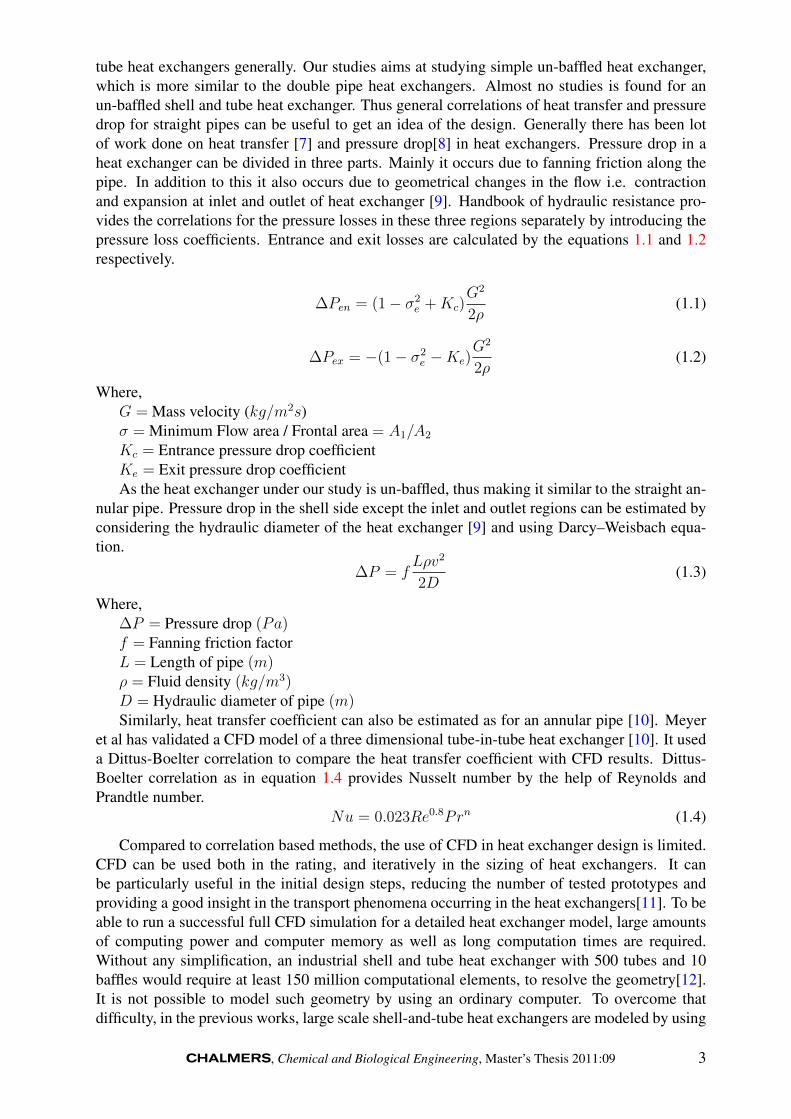
tube heat exchangers generally. Our studies aims at studying simple un-baffled heat exchanger,which is more similar to the double pipe heat exchangers. Almost no studies is found for anun-baffled shell and tube heat exchanger. Thus general correlations of heat transfer and pressuredrop for straight pipes can be useful to get an idea of the design. Generally there has been lotof work done on heat transfer [7] and pressure drop[8] in heat exchangers. Pressure drop in aheat exchanger can be divided in three parts. Mainly it occurs due to fanning friction along thepipe. In addition to this it also occurs due to geometrical changes in the flow i.e. contractionand expansion at inlet and outlet of heat exchanger [9]. Handbook of hydraulic resistance pro-vides the correlations for the pressure losses in these three regions separately by introducing thepressure loss coefficients. Entrance and exit losses are calculated by the equations 1.1 and 1.2respectively.

∆Pen = (1− σ2e +Kc)

G2

2ρ(1.1)

∆Pex = −(1− σ2e −Ke)

G2

2ρ(1.2)

Where,G = Mass velocity (kg/m2s)σ = Minimum Flow area / Frontal area = A1/A2

Kc = Entrance pressure drop coefficientKe = Exit pressure drop coefficientAs the heat exchanger under our study is un-baffled, thus making it similar to the straight an-

nular pipe. Pressure drop in the shell side except the inlet and outlet regions can be estimated byconsidering the hydraulic diameter of the heat exchanger [9] and using Darcy–Weisbach equa-tion.

∆P = fLρv2

2D(1.3)

Where,∆P = Pressure drop (Pa)f = Fanning friction factorL = Length of pipe (m)ρ = Fluid density (kg/m3)D = Hydraulic diameter of pipe (m)Similarly, heat transfer coefficient can also be estimated as for an annular pipe [10]. Meyer

et al has validated a CFD model of a three dimensional tube-in-tube heat exchanger [10]. It useda Dittus-Boelter correlation to compare the heat transfer coefficient with CFD results. Dittus-Boelter correlation as in equation 1.4 provides Nusselt number by the help of Reynolds andPrandtle number.

Nu = 0.023Re0.8Prn (1.4)

Compared to correlation based methods, the use of CFD in heat exchanger design is limited.CFD can be used both in the rating, and iteratively in the sizing of heat exchangers. It canbe particularly useful in the initial design steps, reducing the number of tested prototypes andproviding a good insight in the transport phenomena occurring in the heat exchangers[11]. To beable to run a successful full CFD simulation for a detailed heat exchanger model, large amountsof computing power and computer memory as well as long computation times are required.Without any simplification, an industrial shell and tube heat exchanger with 500 tubes and 10baffles would require at least 150 million computational elements, to resolve the geometry[12].It is not possible to model such geometry by using an ordinary computer. To overcome thatdifficulty, in the previous works, large scale shell-and-tube heat exchangers are modeled by using

, Chemical and Biological Engineering, Master’s Thesis 2011:09 3

some simplifications. The commonly used simplifications are the porous medium model and thedistributed resistance approach. Shell-and-tube heat exchangers can be modeled using distributedresistance approach[12]. By using this method, a single computational cell may have multipletubes; therefore, shell side of the heat exchanger can be modeled by relatively coarse grid. Kao etal [13] developed a multidimensional, thermal-hydraulic model in which shell side was modeledusing volumetric porosity, surface permeability and distributed resistance methods. In all ofthese simplified approaches, the shell side pressure drop and heat transfer rate results showedgood agreement with experimental data.

With the simplified approaches, one can predict the shell side heat transfer coefficient andpressure drop successfully, however for visualization of the shell side flow and temperature fieldsin detail, a full CFD model of the shell side is needed. With ever increasing computationalcapabilities, the number of cells that can be used in a CFD model is increasing. Now it ispossible to model an industrial scale shell- and-tube heat exchanger in detail with the availablecomputers and softwares. By modeling the geometry as accurately as possible, the flow structureand the temperature distribution inside the shell can be obtained. This detailed data can be usedfor calculating global parameters such as heat transfer coefficient and pressure drop that can becompared with the correlation based or experimental ones[6]. Moreover, the data can also beused for visualizing the flow and temperature fields which can help to locate the weaknesses inthe design such as recirculation and re-laminarization zones.

According to a recent review [14], commercial and non commercial softwares are used tomodel different types of heat exchangers. Normally, for modeling the flow, two equation modelsare the most commonly used models. k − ε models are mostly used in industrial designs alongwith wall functions. Jae et al [15] compared the different near wall treatment methods for highReynolds number flows. It was found that non-equilibrium wall functions along with k − εmodels predicts the reattachment lengths more accurately, but two layer model represents theoverall flow domain much better. The use of these near wall treatments is very much dependentupon the choice of turbulence model used.

1.3 Tubular Heat Exchanger

1.3.1 Heat Transfer

Heat transfer is considered to be the basic process of all process industries. During the processof heat transfer, one fluid at higher temperature transfers its energy in the form of heat to theother fluid at a lower temperature. Fluid can transfer its heat through different mechanisms.These mechanisms of heat transfer are conduction, convection and radiation. Radiation is not socommon mode of heat transfer in process industries but in some processes it plays a vital role inheat transfer for example in combustion furnace. Other two modes of heat transfer i.e conductionand convection are most encountered modes of heat transfer in process industries[16][4].

Overall energy balance of a heat transfer system can be generalized by the Equations 1.5 and1.6.

Qh = mhCp (Th,i − Th,o) (1.5)

Qc = mcCp (Tc,o − Tc,i) (1.6)

In actual heat provided by a hotter fluid to the fluid at low temperature is not exactly equaldue to losses and resistances in the form of wall fouling. Assumption is made that the amountof heat transfered from the hotter fluid is equal to the amount of heat transfered to the colderfluid. Usually, heat exchangers are made isolated to minimize the environmental losses. So wecan write as under,


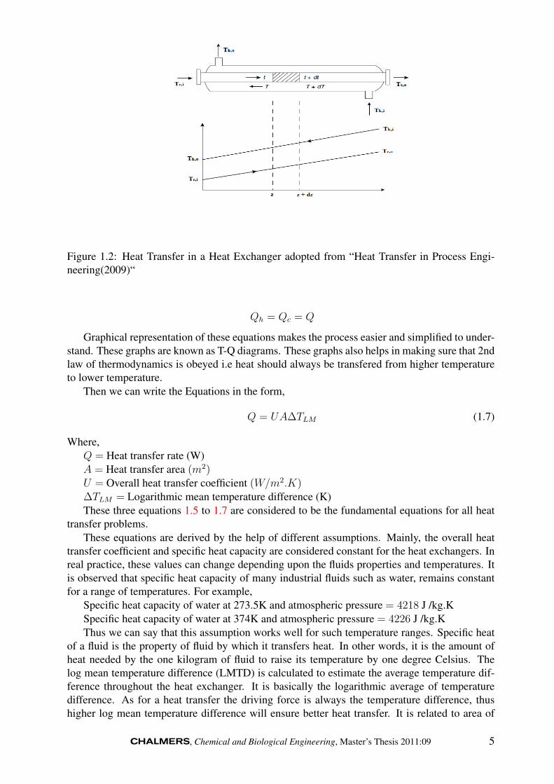
Figure 1.2: Heat Transfer in a Heat Exchanger adopted from “Heat Transfer in Process Engi-neering(2009)“

Qh = Qc = Q

Graphical representation of these equations makes the process easier and simplified to under-stand. These graphs are known as T-Q diagrams. These graphs also helps in making sure that 2ndlaw of thermodynamics is obeyed i.e heat should always be transfered from higher temperatureto lower temperature.

Then we can write the Equations in the form,

Q = UA∆TLM (1.7)

Where,Q = Heat transfer rate (W)A = Heat transfer area (m2)U = Overall heat transfer coefficient (W/m2.K)∆TLM = Logarithmic mean temperature difference (K)These three equations 1.5 to 1.7 are considered to be the fundamental equations for all heat

transfer problems.These equations are derived by the help of different assumptions. Mainly, the overall heat

transfer coefficient and specific heat capacity are considered constant for the heat exchangers. Inreal practice, these values can change depending upon the fluids properties and temperatures. Itis observed that specific heat capacity of many industrial fluids such as water, remains constantfor a range of temperatures. For example,

Specific heat capacity of water at 273.5K and atmospheric pressure = 4218 J /kg.KSpecific heat capacity of water at 374K and atmospheric pressure = 4226 J /kg.KThus we can say that this assumption works well for such temperature ranges. Specific heat

of a fluid is the property of fluid by which it transfers heat. In other words, it is the amount ofheat needed by the one kilogram of fluid to raise its temperature by one degree Celsius. Thelog mean temperature difference (LMTD) is calculated to estimate the average temperature dif-ference throughout the heat exchanger. It is basically the logarithmic average of temperaturedifference. As for a heat transfer the driving force is always the temperature difference, thushigher log mean temperature difference will ensure better heat transfer. It is related to area of


heat exchanger in a way that higher LMTD will cause less heat transfer area and lower LMTDwill need larger heat transfer area. Generally, LMTD is a process condition and one cannot domuch about it as inlet and outlet temperatures of fluids are usually pre decided for a heat ex-changer design. Area can certainly be reduced by making the full use of available LMTD byefficient heat transfer.

1.3.2 Overall Heat Transfer CoefficientThe overall heat transfer of heat exchangers is the ability of transferring heat through differentresistances, It depends upon, the properties of the process fluids, temperatures, flow rates andgeometrical arrangement of the heat exchanger. For example, the number of passes, number ofbaffles and baffle spacing etc. It is defined by the Equation 1.8. This equation basically sumsup all the resistances encountered during the heat transfer and taking the reciprocal gives us theoverall heat transfer coefficient[16].

1

U=

1

hh+

∆x

k+

1

hc+Rf (1.8)

Where:hh = Hot side heat transfer coefficient (W/m2.K)hc = Cold side heat transfer coefficient (W/m2.K)∆x = Exchanger tube wall thickness (m)k = Exchanger wall material thermal conductivity (W/m.K)Rf = Fouling coefficient (W/m2.K) The equation for the overall heat transfer coefficient

can be written as the equation 1.9.

1

U=

1

hh+

1

hc+Rf (1.9)

hh and hc are the individual film coefficients and are defined as the measure of heat transfer forunit area and unit temperature difference. These are calculated separately for both outside andinside fluids. The temperature difference of average temperature of bulk fluid (hot and cold)and wall temperature (inside and outside) is the driving force for the respective fluids. ∆x/k isusually ignored as it doesn’t have a significant effect on the over all heat transfer coefficient.[16].


Chapter 2

Mathematical background and CFD

In this chapter, the governing equations solved by FLUENT and the turbulence models used forthis simulation are explained. Two equation models are used for the simulations. Flow equationsand energy equations are described in detail. The wall treatment methods are also discussed andhow they are important for modeling the heat transfer is also described.

2.1 Flow Calculation

The flow is governed by the continuity equation, the energy equation and Navier-Stokes mo-mentum equations. Transport of mass, energy and momentum occur through convective flowand diffusion of molecules and turbulent eddies. All equations are set up over a control volumewhere i, j, k = 1, 2, 3 correspond to the three dimensions[17].

2.1.1 Continuity Equation

The continuity equation describes the conservation of mass and is written as in equation

∂ρ

∂t+∂ρU1

∂x1

+∂ρU2

∂x2

+∂ρU3

∂x3

= 0 (2.1)

or∂ρ

∂t+∂ρUi∂xi

= 0, i = 1, 2, 3

Equation 2.1 defines the rate of increase of mass in a control volume as equal to the amountthrough its faces. Whereas, for constant density continuity equation is reduced to

∂Ui∂xi

= 0, i = 1, 2, 3

2.1.2 Momentum Equations (Navier-Stokes Equations)

The momentum balance, also known as the Navier-Stokes equations, follows Newton’s secondlaw: The change in momentum in all directions equals the sum of forces acting in those direc-tions. There are two different kinds of forces acting on a finite volume element, surface forcesand body forces. Surface forces include pressure and viscous forces and body forces includegravity, centrifugal and electro-magnetic forces[17].

The momentum equation in tensor notation for a Newtonian fluid can be written as in equa-tion 2.2

7

∂Ui∂t

+ Uj∂Ui∂xj

= −1

ρ

∂P

∂xi+ ν

∂

∂xj(∂Ui∂xj

+∂Uj∂xi

) + gi (2.2)

The equation2.2 can be written in different forms for constant density and viscosity since

ν∂

∂xj(∂Ui∂xj

+∂Uj∂xi

) = ν∂2Ui∂xj∂xi

in incompressible flow. In addition to gravity, there can be

further external sources that may effect the acceleration of fluid e.g. electrical and magneticfields. Strictly it is the momentum equations that form the Navier-Stokes equations but some-times the continuity and momentum equations together are called the Navier-Stokes equations.The Navier-Stokes equations are limited to macroscopic conditions.[17].

The continuity equation is difficult to solve numerically. In CFD programs, the continuityequation is often combined with momentum equation to form Poisson equation 2.3. For constantdensity and viscosity the new equation can be written as below.

∂

∂xi(∂P

∂xi) = − ∂

∂xi(∂(ρUiUj)

∂xj) (2.3)

This equation has more suitable numerical properties and can be solved by proper iteration meth-ods.

2.1.3 Energy EquationEnergy is present in many forms in flow i.e. as kinetic energy due to the mass and velocity of thefluid, as thermal energy, and as chemically bounded energy. Thus the total energy can be definedas the sum of all these energies[17].

h = hm + hT + hC + Φ (2.4)

hm = 12ρUiUi Kinetic energy

hT =∑

nmn

∫ TTref

Cp,ndT Thermal energyhC =

∑nmnhn Chemical energy

Φ = gixi Potential energy

In the above equations mn and Cp,n are the mass fraction and specific heat for species n. Thetransport equation for total energy can be written by the help of above equations. The couplingbetween energy equations and momentum equations is very weak for incompressible flows, thusequations for kinetic and thermal energies can be written separately. The chemical energy is notincluded because there was no species transport involved in this project.

The transport equation for kinetic energy can be written as under,

∂(hm)

∂t= −Uj

∂(hm)

∂xj+ P

∂Ui∂xi− ∂(PUi)

∂xi− ∂

∂xj(τijUi)− τij

∂Ui∂xj + ρgUi

(2.5)

The last term in the equation 2.5 is the work done by the gravity force. Similarly, a balancefor heat can be formulated generally by simply adding the source terms from the kinetic energyequation.

∂(ρCpT )

∂t= −Uj

∂(ρCpT )

∂xj+ keff

∂2T

∂xjxj− P ∂Uj

∂xj+ τkj

∂Uk∂xj

(2.6)

The term on left side of the equation is accumulation term. The first on the right is convectionterm, second is the conduction, third expansion and last is dissipation term. Here the terms in theequation for transformation between thermal and kinetic energy, i.e. expansion and dissipationoccur as source terms.


2.2 Turbulence Modeling

Definition of TurbulenceTurbulent flows have some characteristic properties which distinct them from laminar flows[17].

• The motions of the fluid in a turbulent flow are irregular and chaotic due to random move-ments by the fluid. The flow has a wide range of length, velocity and time scales.

• Turbulence is a three dimensional diffusive transport of mass, momentum and energythrough the turbulent eddies that result in faster mixing rates.

• Energy has to be constantly supplied or the turbulent eddies will decay and the flow willbecome laminar, the kinetic energy becomes internal energy.

Turbulence arises due to the instability in the flow. This happens when the viscous dampeningof the velocity fluctuations is slower than the convective transport, i.e. the fluid element can rotatebefore it comes in contact with wall that stops the rotation. For high Reynolds numbers thevelocity fluctuations cannot be dampened by the viscous forces and the flow becomes turbulent.

Turbulent flows contain a wide range of length, velocity and time scales and solving allof them makes the costs of simulations large. Therefore, several turbulence models have beendeveloped with different degrees of resolution. All turbulence models have made approxima-tions simplifying the Navier-Stokes equations. There are several turbulence models availablein CFD-softwares including the Large Eddy Simulation (LES) and Reynolds Average Navier-Stokes (RANS). There are several RANS models available depending on the characteristic offlow, e.g., Standard k− ε model, k− ε RNG model, Realizable k− ε, k−ω and RSM (ReynoldsStress Model) models.

2.2.1 Turbulence ModelThe RANS models assume that the variables can be divided into a mean and fluctuating part.The pressure and velocity are then expressed as .

Ui = 〈Ui〉+ ui

Pi = 〈Pi〉+ pi

where the average velocity is defined as

〈Ui〉 =1

2T

∫ T

−TUidt

The decomposition of velocity and pressure inserted into Navier-Stokes equations gives

∂〈Ui〉∂t

+ 〈Ui〉∂〈Ui〉∂xj

= −1

ρ

∂

∂xj

{〈P 〉δij + µ

(∂Ui∂xj

+∂Uj∂xi

)− ρ〈uiuj〉

}(2.7)

The last term −ρ〈uiuj〉 is called the Reynolds stresses and describes the velocity fluctuationscaused by turbulence. This term needs to be modeled to close this equation.

The Reynolds averaged stress models use the Boussinesq approximation which is basedon the assumption that the Reynolds stresses are proportional to mean velocity gradient. TheBoussinesq approximation assumes that the eddies behave like the molecules, that the turbulenceis isotropic and that the stress and strain are in local equilibrium. These assumptions cannotbe made for certain flows, e.g., the highly swirling flows having a large degree of anisotropic


turbulence and then inaccurate results are obtained. The Boussinesq approximation allows theReynolds stresses to be modeled using a turbulent viscosity which is analogous to the molecularviscosity[17]. Thus above equation becomes,

∂〈Ui〉∂t

+ 〈Ui〉∂〈Ui〉∂xj

= −1

ρ

∂〈P 〉∂xi

− 2

3

∂k

∂xi+

∂

∂xj

[(ν + νT )

(∂Ui∂xj

+∂Uj∂xi

)](2.8)

The use of RANS models requires that two additional transport equations, for the turbulencekinetic energy, k, and the turbulence dissipation rate, ε, or the specific dissipation rate, ω, aresolved.

2.2.2 Two-Equations ModelsDifferent turbulence models can be classified on the basis of number of extra equations used toclose the set of equations. There are zero, one and two equations models which are commonlyemployed for turbulence modeling. Zero equation model makes a simple assumption of constantviscosity (Prandtl’s mixing length model). Whereas one equation model assumes that viscosityis related to history effects of turbulence by relating to time average kinetic energy.Similarly, twoequation model uses two equations to close the set of equations. These two equations can modelturbulent velocity or turbulent length scales. There are many variables which can be modeled forexample vorticity scale,frequency scale,time scale and dissipation rate. Among these variables,dissipation rate ε is the most commonly used variable. This model is named with respect to thevariables being modeled. For example k − ε model, as it models k (Turbulent kinetic energy)and k − ε(Turbulent energy dissipation rate). Another, important turbulence model is k − ωmodel. It models k (Turbulent kinetic energy) and ω (Specific dissipation rate). These modelshave become now common in industrial use. These provide significant amount of reliability asthey use two variables to close the set of equations[18].

k − ε Models

The first transported variable is turbulent kinetic energy, k. The second transported variable inthis case is the turbulent dissipation, ε. There respective modeled transport equations are asunder,

For k,

∂k

∂t+〈Uj〉

∂k

∂xj= νT

[(∂〈Ui〉∂xj

+∂〈Uj〉∂xi

)∂〈Ui〉∂xj

]−ε +

∂

∂xj

[(ν + νT

σk

) ∂k

∂xj

]And for ε

∂ε

∂t+〈Uj〉

∂ε

∂xj= Cε1νT

ε

k

[(∂〈Ui〉∂xj

+∂〈Uj〉∂xi

)∂〈Ui〉∂xj

]+Cε2

ε2

k+

∂

∂xj

[(ν +

νTσε

)∂ε

∂xj

]1 2 3 4 5

The physical interpretation of the ε equation is,

1. Accumulation of ε

2. Convection of ε by the mean velocity

3. Production of ε


4. Dissipation of ε

5. Diffusion of ε

The time constant for turbulence is calculated from the turbulent kinetic energy and dissipationrate of turbulent kinetic energy.

τ =k

εNote that the source term in ε equation is same as in the k-equation divided by the time

constant τ and the rates of dissipation ε is proportional toε

τ=ε2

k.

The turbulent viscosity must be calculated to close the k−εmodel. As the turbulent viscosityis given as the product between characteristic length and velocity scales, νT ∝ ul. This means

that, νT = Cµk2

ε.

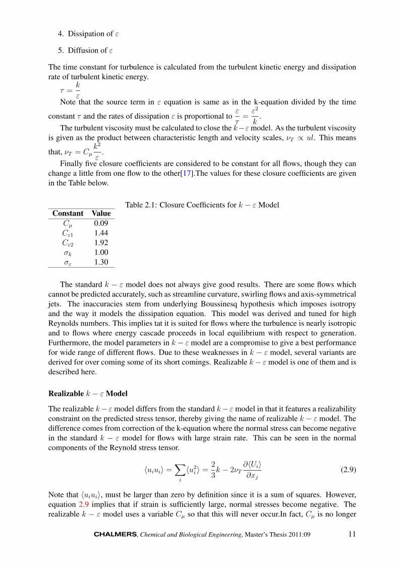
Finally five closure coefficients are considered to be constant for all flows, though they canchange a little from one flow to the other[17].The values for these closure coefficients are givenin the Table below.

Table 2.1: Closure Coefficients for k − ε ModelConstant Value

Cµ 0.09Cε1 1.44Cε2 1.92σk 1.00σε 1.30

The standard k − ε model does not always give good results. There are some flows whichcannot be predicted accurately, such as streamline curvature, swirling flows and axis-symmetricaljets. The inaccuracies stem from underlying Boussinesq hypothesis which imposes isotropyand the way it models the dissipation equation. This model was derived and tuned for highReynolds numbers. This implies tat it is suited for flows where the turbulence is nearly isotropicand to flows where energy cascade proceeds in local equilibrium with respect to generation.Furthermore, the model parameters in k− ε model are a compromise to give a best performancefor wide range of different flows. Due to these weaknesses in k − ε model, several variants arederived for over coming some of its short comings. Realizable k− ε model is one of them and isdescribed here.

Realizable k − ε Model

The realizable k− ε model differs from the standard k− ε model in that it features a realizabilityconstraint on the predicted stress tensor, thereby giving the name of realizable k − ε model. Thedifference comes from correction of the k-equation where the normal stress can become negativein the standard k − ε model for flows with large strain rate. This can be seen in the normalcomponents of the Reynold stress tensor.

〈uiui〉 =∑i

〈u2i 〉 =

2

3k − 2νT

∂〈Ui〉∂xj

(2.9)

Note that 〈uiui〉, must be larger than zero by definition since it is a sum of squares. However,equation 2.9 implies that if strain is sufficiently large, normal stresses become negative. Therealizable k − ε model uses a variable Cµ so that this will never occur.In fact, Cµ is no longer


constant, instead it is a function of the local state of flow to ensure that the normal stresses arepositive under all flow conditions, i.e. to ensure that normal stresses are positive under all flowconditions. Realizability also means that the stress tensor satisfies 〈u2

i 〉〈u2j〉 − 〈uiuj〉2 ≥ 0, i.e.

the Schwartz’s inequality is fulfilled. Hence, the model is likely to to provide better performancefor flows involving rotation and separation. It is noteworthy that the realizable model is bettersuited to flows where the strain rate is large. This includes the flows with strong streamlinecurvature and rotation. Validation of complex flows, e.g. boundary layer flows, separated flowsand rotating shear flows show that the realizable k − ε model performs better than the standardk − ε model[17][18].

k − ω SST Model

It has been a problem to accurately predict the flow separation. It is seen that standard modelusually predicts the separation too late and length of separation is not accurately predicted. Forthis reason, near wall region becomes very important and critical in such situations. The k − ωSST turbulence model is a two equation model. This model is known because it uses both k− ωand k − ε models. In a simple k − ω model, specific dissipation energy is modeled along withturbulent kinetic energy.

The modeled equation for k is as under.

∂k

∂t+ 〈Uj〉

∂k

∂xj= νT

[(∂〈Ui〉∂xj

+∂〈Uj〉∂xi

)∂〈Ui〉∂xj

]− βkω +

∂

∂xj

[(ν +

νTσk

)∂k

∂xj

](2.10)

and the modeled equation for ω is

∂ω

∂t+〈Uj〉

∂ω

∂xj= α

ω

kνTε

k

[(∂〈Ui〉∂xj

+∂〈Uj〉∂xi

)∂〈Ui〉∂xj

]−β∗ω2+

∂

∂xj

[(ν +

νTσω

)∂ω

∂xj

](2.11)

The turbulent viscosity can be estimated from νT =k

ω. This model is superior to standard

models in a way that it models the region of low turbulence better where turbulent kinetic energyand dissipation energy both approach to zero. Whereas, the k − ω model is good in near wallregions and doesn’t need the wall functions. Thus this model performs good in viscous sublayer.Due to this, it demands very fine mesh near wall, such that first grid is kept at a y+ < 5. Closurecoefficients for k − ω model can be seen in Table 2.2.2.

Table 2.2: Closure Coefficients for k − ω ModelConstant Value

α 5/9β 3/40β∗ 9/100σk 1/2σω 1/2

SST models stands for Shear Stress Transport model, it is the combination of k−ω and k−εmodels. As k − ε is a high Reynolds number model thus in the near wall region k − ω modelis used. Whereas, in the region away from the walls, k − ε model is used. The SST modeluses a blending function whose value depends upon the distance from the walls. Near the wall,in viscous sublayer, this blending function is one and only k − ω model is used. The regionsaway from the wall this function is zero and uses only k − ε model. This model also includesthe cross diffusion term. In this model turbulent viscosity is changed to include the effect of


turbulent shear stress transport. Modeling constants are also different from other models. Thesecharacteristics make the SST model reliable for the adverse pressure gradient flows and boundarylayer separation. Details can be seen in the Fluent user guide [19].

2.3 Wall Treatment MethodsThe near-wall modeling considerably effects the reliability of numerical solutions, because wallsare the major cause of mean vorticity and turbulence. Near the wall, gradients of variable suchas velocity and pressure are high and other scalar variables also undergo sudden increase ordecrease. So, precise estimation of flow variables in these regions is of major concern, whichwill lead to good predictions of turbulence as well.[19].

It is known that the region near wall can be divided into three sub sections. The section/layernext to the wall is named as viscous sub-layer. The flow in this layer is entirely laminar andmolecular viscosity is major factor in calculating the heat and momentum transfer. In this regionturbulent viscosity assumption is not valid at all. While, the section farthest from the wall insidethe near wall region, is called the fully turbulent layer. Here the assumption of turbulent viscosityis valid and turbulence has a major effect over the heat and momentum transport. Then there is atransition region in between these two sections called buffer layer. In this layer, both molecularand turbulent viscosity is important[19].

Modeling of the near wall region can be achieved by fully resolving the region all the wayto the wall. This approach may need very fine mesh near the wall and would definitely needhuge computational resources to solve. There is another approach, in which near wall regionis not resolved completely and empirical formulas are used to guess the variables at the wall.These empirical formulas are called the wall functions. Wall functions are applied on a pointaway from the wall outside the viscous sublayer. These wall functions are used to connect theturbulent regions with the viscous sublayer[19]. Graphical representation of these both methodscan be seen in the Figure 2.1.

2.3.1 Wall FunctionsWall functions are a set of empirical formulas which connects the different variables such as ve-locity, temperature and pressure at the wall to the near wall region (Turbulence boundary layer).Wall functions are applied by using the law of wall for the variables near the wall region. Thenthey formulate the turbulence variables such as turbulent kinetic energy and turbulent dissipationenergy. These formulations depend upon the respective turbulence model. There are followingtypes of wall functions mostly used.

• Standard Wall Functions

• Non-Equilibrium Wall Functions

• Enhanced Wall Functions

Standard Wall Functions

Wall functions basically do not resolve the boundary layer. Thus in their true sense, these arenot exact solution to any problem. Wall functions make it possible to calculate the boundarycondition away from the wall. Use of wall functions permit the solution at a point where wallfunctions are suitable, rather than on the wall itself. The boundary conditions are then used atthis point and wall functions compute the rapid variation of the flow variables which arise inclose proximity to the wall region to be accounted for without resolving the viscous layer next


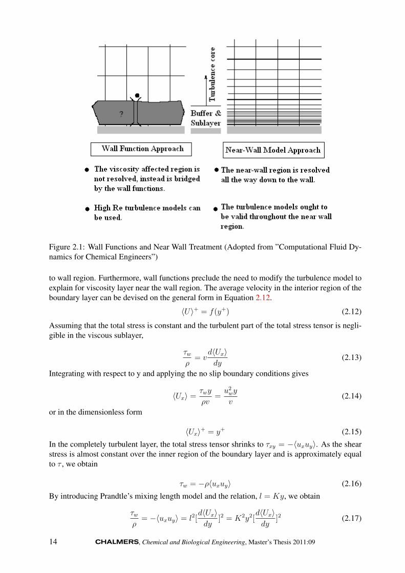
Figure 2.1: Wall Functions and Near Wall Treatment (Adopted from ”Computational Fluid Dy-namics for Chemical Engineers”)

to wall region. Furthermore, wall functions preclude the need to modify the turbulence model toexplain for viscosity layer near the wall region. The average velocity in the interior region of theboundary layer can be devised on the general form in Equation 2.12.

〈U〉+ = f(y+) (2.12)

Assuming that the total stress is constant and the turbulent part of the total stress tensor is negli-gible in the viscous sublayer,

τwρ

= vd〈Ux〉dy

(2.13)

Integrating with respect to y and applying the no slip boundary conditions gives

〈Ux〉 =τwy

ρv=u2wy

v(2.14)

or in the dimensionless form

〈Ux〉+ = y+ (2.15)

In the completely turbulent layer, the total stress tensor shrinks to τxy = −〈uxuy〉. As the shearstress is almost constant over the inner region of the boundary layer and is approximately equalto τ , we obtain

τw = −ρ〈uxuy〉 (2.16)

By introducing Prandtle’s mixing length model and the relation, l = Ky, we obtain

τwρ

= −〈uxuy〉 = l2[d〈Ux〉dy

]2 = K2y2[d〈Ux〉dy

]2 (2.17)


As the characteristic velocity scale for the sub-layers is given by u∗ =√τw/ρ. Equation 2.17

can now be written as

u2∗ = K2y2[

d〈Ux〉dy

]2 (2.18)

Taking the square root of the both sides and integrating with respect to y we obtain the logarith-mic velocity profile, which in dimensionless form reads

〈Ux〉+ =1

Kln(y+) +B (2.19)

where k ≈ 0.42 and B ≈ 5.0 (K is Von Karman constant). Equation 2.19 is referred to aslogarithmic law of wall or simply the log law. Thus in the viscous sub-layer velocity varieslinearly with y+, whereas it approaches the log law in the buffer sub-layer as shown in Figure2.3.1 below.

Figure 2.2: The Law of Wall (Adopted from ”Computational Fluid Dynamics for ChemicalEngineers”)

In addition of the logarithmic profile for the average velocity, the wall functions also consistsof equation for the near wall turbulent quantities.There is no transport of k to the wall while εoften has the maximum at the wall. In the derivation of boundary conditions for the turbulentquantities, it is assumed that flow is in local equilibrium which means that production equalsdissipation. The boundary condition for k is given by Equation 2.20.

k =u2∗

C1/2µ

(2.20)

and for ε by,

ε =u3∗ky

(2.21)

The use of wall functions requires that the first grid point adjacent to the wall is within thelogarithmic region. In dimensionless distance, that is 30 < y+ < 100. Upper limit of y+ can be


as high as 300 but it should not exceed 300. Thus it can be said that use of standard wall functionsrequires y+ values between 30 and 300. The log-law has proven very useful as a universal forthe inner region of the flat plate turbulent boundary layer and has been experimentally verifiedin numerous studies. However, wall functions are not as valid under the conditions of strongpressure gradients, separated and impinging flows. In these situations standard wall functionsare not appropriate choice[19].

Non-equilibrium Wall Functions

Non equilibrium wall functions are commonly used for the non-equilibrium turbulent boundaryconditions. In such conditions assumption of local equilibrium between production and dissipa-tion is not valid. Standard wall functions are based on this primary assumptions, thus limitingtheir use in these conditions. In boundary layer experiencing an adverse pressure gradient, thefluid closest to the wall is retarded due to the pressure increase in the stream wise direction. Asa result, wall shear stress is decreased. Consequently, adverse pressure gradients alter the meanvelocity profile as well as the turbulence in the boundary layer.This means that when the pressuregradient is high, the logarithmic boundary layer representation cannot be used. Hence, severalflows e.g flow separation, reattachment, strong pressure gradients and flow impinging on a wall,the flow situation departs significantly from the ideal conditions and accuracy of the standardwall functions is low.

Modified wall functions which are capable to some extent in accounting for effects of pres-sure gradients and departure from equilibrium have been developed. By using such modified wallfunctions, for non-equilibrium boundary layers, improved predictions can be obtained. Thesewall functions typically consist of a log-law for the mean velocity, which is sensitized to pres-sure gradients effects. Boundary conditions for the turbulence quantities are derived based onmethods where equilibrium condition is relaxed. Thus, these modifications further extend theapplicability of the wall function approach and allows improvements to be obtained for complexflow conditions.

When the near wall region is of particular interest and the conditions are very non-ideal, itmay be necessary to resolve the viscosity affected near wall region in detail. Such simulations,require dense meshes and modifications of high Reynolds number model since they are not validin the near wall region[19].

Enhanced Wall Treatment

Improved modeling of wall bounded flows can be achieved using a two layer zonal approach orsing Low Reynolds number turbulence models. These techniques permit governing equationsto be solved all the way to the wall, thereby eliminating the use of wall functions. It improvesthe predictions of wall shear stress and wall hear transfer. Resolution of the near wall region in-cluding the viscous sub-layer requires a very fine near wall grid resolution. Hence this modelingapproach requires larger computational power compared to the wall function approach[19].

Two Layer Zonal Modeling

In the two layer zonal approach, the domain is divided into two zones or regions as the nameimplies. These two regions may be identified by the wall distance based Reynolds number.

Rey = y

√k

v(2.22)

where y is the distance to the nearest wall.The fully turbulent region is normally taken as Rey > 200 and the viscosity affected region as


Rey < 200. In the viscosity affected near wall region, a one equation turbulence model for theturbulent kinetic energy is applied and an algebraic relationship is used to calculate the energydissipation rate. Whereas, a two-equation model such as standard or an advanced k − ε modelis used in the completely turbulent region. Thus, in the viscous zone the energy dissipation iscalculated from,

ε =k3/2

lε(2.23)

where lε is an appropriate length scale.It is common practice to use a blending function to calculate the viscosity in the transition re-gion. This function simply blends the turbulent viscosity in the viscosity affected region with theturbulent viscosity in turbulent region to obtain a smooth transition. Thus blending function isdefined as unity far from the wall and zero at the wall. The two layer zonal approach requiresapproximately the same boundary layer resolution as the low Reynolds number approach. Sincethe dissipation energy is calculated from an algebraic equation, this approach may be more stablecompared to the low Reynolds number approach[19].

Low Reynolds Number Turbulence Models

One way of characterizing a turbulence model is to distinguish between high and low Reynoldsnumber models. In the former, wall functions are used to approximate the turbulence quantitiesnear the walls. The standard k − ε model is an example of high Reynolds number model.Thesemodels are not valid near the wall region. Low Reynolds number models are examples of themodels which are also valid in the viscous wall region and can thus be integrated all the way tothe wall.

The low Reynolds number modifications typically consist of dampening functions for thesource terms in the transport equation for ε and in the expression for turbulent viscosity. Thesemodifications allow the equations to be integrated through the turbulent boundary layer, includingthe viscous sub-layer, thereby giving better prediction for near wall flows. It is important to pointout that these models are applicable for high global Reynolds numbers. For that a transitionmodel is needed. It should also be noted that these models are of ad-hoc nature and cannot berelied upon to give consistently good results for all type of flows. Examples of low Reynoldsnumber variants of k − ε model are the Launder-Sharma, Lam-Bremhorst and several othermodels.

For low Reynolds number models, the general transport equations for k are given by Equation2.24

∂k

∂t+ 〈Uj〉

∂k

∂xj=

∂

∂xj{(v +

vtσk

)∂k

∂xj}+ vt{(

∂〈Ui〉∂xj

+∂〈Uj〉∂xi

)∂〈Ui〉∂xj} − ε (2.24)

and the general transport equations for ε are given by Equation 2.25.

∂ε′

∂t+ 〈Uj〉

∂ε′

∂xj=

∂

∂xj{(v +

vtσε

)∂ε

′

∂xj}+ C1εf1vt

ε′

k{(∂〈Ui〉

∂xj+∂〈Uj〉∂xi

)∂〈Ui〉∂xj} − C2εf2

ε′2

k+ E

(2.25)where the turbulent viscosity is calculated by

vT = fµCµk2

ε′(2.26)

and the energy dissipation, ε, is related to ε′ by Equation 2.27.

ε = ε0 + ε′

(2.27)


The quantities ε0 and E are defined differently for each model, ε0 is the value of ε at the wall.The difference between these models and the standard k − ε is the dampening functions f1 andf2 in the equation of ε and the dampening function fµ. The dampening functions are generallywritten in terms of specifically defined Reynolds numbers, such as in Equations 2.28 and 2.29.

Ret =k2

vε(2.28)

and

Rey =

√ky

v(2.29)

Obviously the global Reynolds number has nothing to do with the low Reynolds number turbu-lent models. The low Reynolds number comes from the local Reynolds number[19].


Chapter 3

CFD Analysis

Computational fluid dynamic study of the system starts with building desired geometry and meshfor modeling the domain. Generally, geometry is simplified for the CFD studies. Meshing isthe discretization of the domain into small volumes where the equations are solved by the helpof iterative methods. Modeling starts with defining the boundary and initial conditions for thedomain and leads to modeling the entire system domain.Finally, it is followed by the analysis ofthe results.

3.1 GeometryHeat exchanger geometry is built in the ANSYS workbench design module. Geometry is sim-plified by considering the plane symmetry and is cut half vertically. It is a counter current heatexchanger, and the tube side is built with 11 separate inlets comprising of 8 complete tubes and3 half tubes considering the symmetry. The shell outlet length is also increased to facilitate themodeling program to avoid the reverse flow condition. In the Figure 3.1, the original geometryalong with the simplified geometry can be seen.

(a) Original Geometry (b) Simplified Geometry

Figure 3.1: (a) and (b)

The dimensions of the geometry are also given in the Table 3.1 below.

19

Table 3.1: Heat Exchanger DimensionsNo. Description Unit Value1 Overall dimensions mm 54x378x58502 Shell diameter mm 1083 Tube outer diameter mm 164 Tube inner diameter mm 14.65 Number of tubes 196 Shell/Tube length mm 58507 Inlet length mm 708 Outlet length mm 200

3.2 Mesh

Initially a relatively coarser mesh is generated with 1.8 Million cells. This mesh contains mixedcells (Tetra and Hexahedral cells) having both triangular and quadrilateral faces at the bound-aries. Care is taken to use structured cells (Hexahedral) as much as possible, for this reasonthe geometry is divided into several parts for using automatic methods available in the ANSYSmeshing client. It is meant to reduce numerical diffusion as much as possible by structuring themesh in a well manner, particularly near the wall region. Later on, for the mesh independentmodel, a fine mesh is generated with 5.65 Million cells. For this fine mesh, the edges and regionsof high temperature and pressure gradients are finely meshed.

3.2.1 y+ Values

y+ values play an important role in turbulence modeling for the near wall treatment. For thisreason, inflation on the walls is created to achieve the correct values of y+ values. Requirementsfor the y+ values for different wall treatments are given in the Table 3.3 [20]. It can be seen inthe Table 3.3 that y+ required for the standard and Non-equilibrium wall functions is high.

The tubes inside the shell are very close to each other and thus has very little space in be-tween. In order to resolve the boundary layer sufficiently, 10 to 15 cells are required between theadjacent tube walls. The inflation is thus kept very fine with first cell y+ < 5. This y+ conditionputs a restriction thus limiting the use of standard and non-equilibrium wall functions. For allother walls of the heat exchanger, y+ values are set according to the wall treatment methods re-quirements. So when using Standard and Non-equilibrium wall functions y+ values are less than5 at the tube walls and at all other walls are according to requirements mentioned in Table 3.3.

3.2.2 Grid Independence

The contours from coarser mesh and fine mesh are analyzed and it is noted that fine mesh resolvesthe region of high pressure and temperature gradients better as compared to coarse mesh. Thustaking care of these particular regions, coarse mesh is adapted to resolve these gradients. Thecriterion for adaption are temperature and pressure gradients. It is mainly refined in inlet andoutlet regions to get the better estimations of pressure drop and heat transfer. Rapid mixing ofhot and cold fluids is observed at the outlet, which led to refine the mesh further. Adaptions on thebasis of temperature and pressure gradients are made to the mesh to get a fully grid independentmodel. Aspect ratio of the cells is kept same as coarse mesh because it is checked that the aspectratio doesn’t effect much. Thus finally, mesh contains 2.2 million cells. Different views of allthese meshes can be seen in the Table 3.2. The mesh contained different types of cells but 80%


Table 3.2: Different MeshesMesh Symmetry view Cross-section view

Coarse

Medium

Fine


Table 3.3: y+ Values for Different Wall TreatmentsWall Treatment Method Recommendedy+ values Used y+ values at Tube wallsStandard wall functions 30 < y+ < 400 y+ < 5

Non-equilibrium wall functions 30 < y+ < 100 y+ < 5Low Reynolds number model y+ ∼= 1 y+ < 1

of them are hexahedral cells. Detailed composition of the mesh can be seen in the Pi chart 3.2.2.

Figure 3.2: Mesh Composition

In order to see the grid independence, local velocity and temperature profiles at the shellcross-section are observed and it can be seen in Figures 3.2.2 and 3.2.2. The velocity and tem-perature profile for the coarse mesh is very much different from the profile obtained with Finemesh. Thus, the coarse mesh after adaption is converted to a medium mesh of 2.2 million cellsand its velocity and temperature profiles are in better agreement with fine mesh. Local heat fluxdepends upon temperature and mass flux (velocity of the fluid) in this case, as specific heat anddensity are considered constant. Thus on the basis of above mentioned results, heat flux is alsofound grid independent.


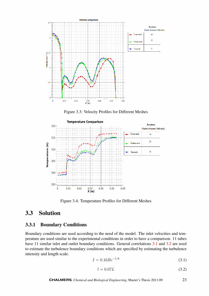
Figure 3.3: Velocity Profiles for Different Meshes

Figure 3.4: Temperature Profiles for Different Meshes

3.3 Solution

3.3.1 Boundary Conditions

Boundary conditions are used according to the need of the model. The inlet velocities and tem-perature are used similar to the experimental conditions in order to have a comparison. 11 tubeshave 11 similar inlet and outlet boundary conditions. General correlations 3.1 and 3.2 are usedto estimate the turbulence boundary conditions which are specified by estimating the turbulenceintensity and length scale.

I = 0.16Re−1/8 (3.1)

l = 0.07L (3.2)


Later it is seen that the turbulence boundary conditions have a very little affect over the resultsand solution. The walls are separately specified with respective boundary conditions. ’No slip’condition is considered for each wall. Except the tube walls, each wall is set to zero heat fluxcondition. The tube walls are set to ’coupled’ for transferring of heat between shell and tube sidefluids. The details about all boundary conditions can be seen in the Table 3.4.

Table 3.4: Boundary ConditionsBC Type Shell Tube

Inlet Velocity-inlet 1.2 m/s 1.8 m/sOutlet Pressure-outlet 0 0Wall No slip condition No heat flux CoupledTurbulence Turbulence Intensity 3.6% 4%

Length Scale 0.005 0.001Temperature Inlet temperature 317K 298KMass flow rate 20000kg/hr 20000kg/hr

3.3.2 Discretization SchemeThere are several discretization schemes to choose from. Initially every model is run with thefirst order upwind scheme and then later changed to the second order upwind scheme. It is doneto have better convergence but changed to higher order scheme to avoid the numerical diffusionIt is seen that the flow is unidirectional in most of the domain. So, it is recommended to usesecond order schemes for strong convection. Second order upwind scheme fulfills the propertyof transportivness and is more accurate than first order scheme. A major drawback of this schemeis its unboundedness which is not the case with first order scheme.

3.3.3 Measure of ConvergenceIt is tried to have a good convergence through out the simulations. The solution time increasesif the convergence criteria is made strict. Good thing about this model is that it doesn’t take toomuch time to converge. Thus a strict criteria is possible to get good accurate results. For thisreason unscaled residuals in ANSYS Fluent which is given as in equation 3.3 are set accordingto Table 3.5.

RΦ =∑cellsP

|∑nb

anbΦnb + b− apΦp| (3.3)

Here Φ is any variable, ap is center coefficient, anb are the influence coefficients from the neigh-boring cells and b is the constant part of the boundary condition.

Table 3.5: ResidualsVariable Residualx-velocity 10−6

y-velocity 10−6

z-velocity 10−6

Continuity 10−6

Specific dissipation energy/ dissipation energy 10−5

Turbulent kinetic energy 10−5

Energy 10−9


Chapter 4

Results and Discussion

4.1 Model Comparison

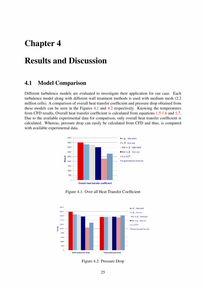
Different turbulence models are evaluated to investigate their application for our case. Eachturbulence model along with different wall treatment methods is used with medium mesh (2.2million cells). A comparison of overall heat transfer coefficient and pressure drop obtained fromthese models can be seen in the Figures 4.1 and 4.2 respectively. Knowing the temperaturesfrom CFD results, Overall heat transfer coefficient is calculated from equations 1.5 1.6 and 1.7.Due to the available experimental data for comparison, only overall heat transfer coefficient iscalculated. Whereas, pressure drop can easily be calculated from CFD and thus, is comparedwith available experimental data.

Figure 4.1: Over all Heat Transfer Coefficient

Figure 4.2: Pressure Drop

25

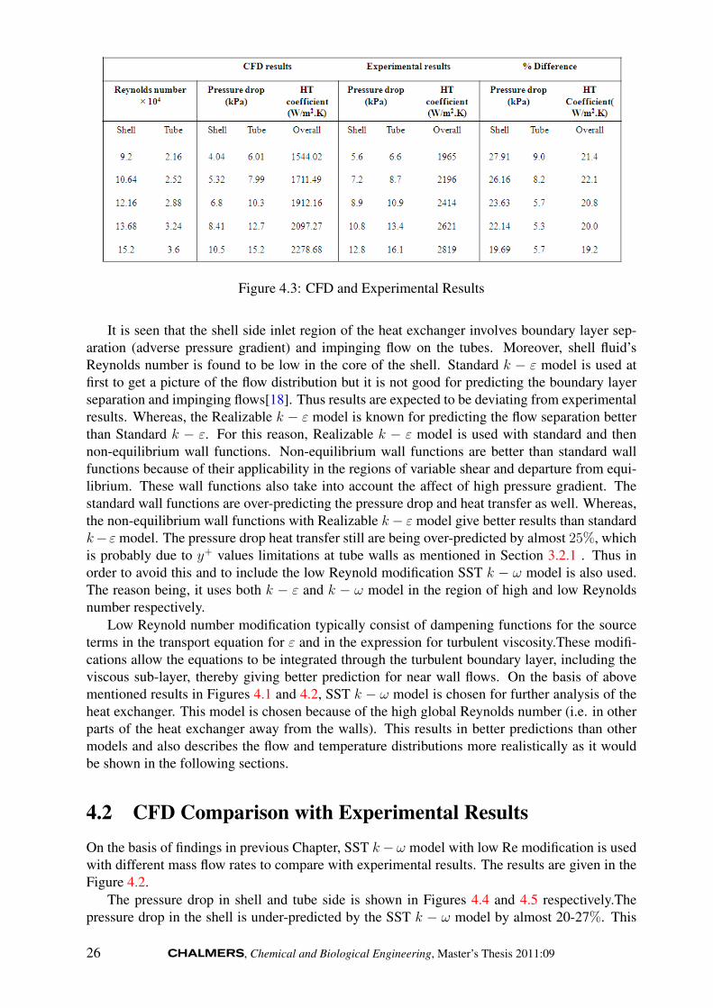
Figure 4.3: CFD and Experimental Results

It is seen that the shell side inlet region of the heat exchanger involves boundary layer sep-aration (adverse pressure gradient) and impinging flow on the tubes. Moreover, shell fluid’sReynolds number is found to be low in the core of the shell. Standard k − ε model is used atfirst to get a picture of the flow distribution but it is not good for predicting the boundary layerseparation and impinging flows[18]. Thus results are expected to be deviating from experimentalresults. Whereas, the Realizable k − ε model is known for predicting the flow separation betterthan Standard k − ε. For this reason, Realizable k − ε model is used with standard and thennon-equilibrium wall functions. Non-equilibrium wall functions are better than standard wallfunctions because of their applicability in the regions of variable shear and departure from equi-librium. These wall functions also take into account the affect of high pressure gradient. Thestandard wall functions are over-predicting the pressure drop and heat transfer as well. Whereas,the non-equilibrium wall functions with Realizable k− ε model give better results than standardk− ε model. The pressure drop heat transfer still are being over-predicted by almost 25%, whichis probably due to y+ values limitations at tube walls as mentioned in Section 3.2.1 . Thus inorder to avoid this and to include the low Reynold modification SST k − ω model is also used.The reason being, it uses both k − ε and k − ω model in the region of high and low Reynoldsnumber respectively.

Low Reynold number modification typically consist of dampening functions for the sourceterms in the transport equation for ε and in the expression for turbulent viscosity.These modifi-cations allow the equations to be integrated through the turbulent boundary layer, including theviscous sub-layer, thereby giving better prediction for near wall flows. On the basis of abovementioned results in Figures 4.1 and 4.2, SST k − ω model is chosen for further analysis of theheat exchanger. This model is chosen because of the high global Reynolds number (i.e. in otherparts of the heat exchanger away from the walls). This results in better predictions than othermodels and also describes the flow and temperature distributions more realistically as it wouldbe shown in the following sections.

4.2 CFD Comparison with Experimental ResultsOn the basis of findings in previous Chapter, SST k− ω model with low Re modification is usedwith different mass flow rates to compare with experimental results. The results are given in theFigure 4.2.

The pressure drop in shell and tube side is shown in Figures 4.4 and 4.5 respectively.Thepressure drop in the shell is under-predicted by the SST k − ω model by almost 20-27%. This


Figure 4.4: Comparison of Shell Side Pressure Drop

Figure 4.5: Comparison of Tube Side Pressure Drop

could be due to the several reasons including complicated geometry of the shell side and nu-merical diffusion. Where as, the pressure drop in tube side (straight tubes) is predicted with anaverage error between 5-9%. It can be due to small baffles in the tubes used in the experimentalsetup.

Overall heat transfer coefficient comparison with experiments can also be seen in the Figure4.6. It is also been under-predicted by this model but still better than other models with anaverage error of 19-20%. The good thing about these results is the constant difference fromexperimental results and consistency with the real systems, i.e. with higher pressure drop, higherheat transfer is achieved.

Figure 4.6: Comparison of Overall Heat Transfer Coefficient

4.3 Contour PlotsThe temperature and velocity distribution along the heat exchanger can be seen through side viewon the plane of symmetry. The contour plots in Figure 4.7 and 4.8 shows the whole length of heat


exchanger. The whole length is too much to be displayed on a single page with understandableresolution, thus it is cut into 4 parts to see it closely. The top most part is the inlet region andlowest part is the outlet.

As the heat exchanger is almost 6 meters long, the velocity and temperature contour plotsacross the cross section at different position along the length of heat exchanger will give an ideaof the flow in detail. For convenience the plots are taken at 5 different positions and the detailsof the temperature distribution in comparison to the velocity distribution can be observed in theTable 4.1.

Figure 4.7: Velocity Contour Plot at Symmetrical Plane

Figure 4.8: Temperature Contour Plot at Symmetrical Plane


Table 4.1: Velocity and Temperature Contour Plots

Velocity Temperature

Inlet

1 m

3 m

5 m

Outlet


4.4 Vector PlotsVelocity vector plots can be seen below in Figures 4.9, 4.10(a) and 4.10(b). These plots givean idea of flow separation at at inlet region and the impingement of the fluid on the tubes. Therecirculation at the inlet region is also obvious from the Figure 4.10(b). The major portion of thefluid tends to move around the tube bundle, and part of the fluid enters the tube bundle throughthe tube spacing as seen in Figure 4.9. This region is a major reason of pressure drop due toimpingement on the tube bundle. At the outlet, boundary layer separation takes place and theflow from the shell tends to mix with each other. This could be a non-symmetric region due tomixing of fluid from all sides.

Figure 4.9: Vector Plot of Velocity at Inlet

(a) Vector Plot of Velocity at Outlet (b) Vector Plot of Velocity at Inlet Recirculation

Figure 4.10: Outlet (a) and Inlet (b)

4.5 ProfilesTemperature and velocity profiles are very useful to understand the heat transfer along with theflow distribution. The temperature profiles are drawn across the cross section and along the length


of heat exchanger at different positions. Whereas, the velocity profiles are drawn only across thecross section. In order to understand the profiles, following Figures 4.11(a) and 4.11(b) must beunderstood first.

(a) Cross-Section (b) Length

Figure 4.11: Profiling(a) and (b)

In Figure 4.11(a), the outer edge of the shell is divided into three different names according totheir positions. Top, bottom and outer middle can be seen in the Figure 4.11(a). Then, the innerfluid is divided into different fluid zones namely A,B, C to H. The temperature profile is drawnat these locations through to the whole length of the heat exchanger. It is done to understandtheir temperature profiles separately along the length of heat exchanger because the shell fluidremains parallel to tubes and doesn’t mix until the outlet region. The tubes are also numbered 1to 11. Where 1 being the inner most tube and 6 to 11 being the outer row of tubes exposed to theouter shell fluid.

In Figure 4.11(b), the yellow lines are drawn across the cross-section (joining the circumfer-ence and center of the shell cross-section). These lines are drawn at different positions in theheat exchanger, where temperature and velocity profiles are drawn.

4.5.1 Velocity ProfileBefore going into detailed discussions, velocity profile is examined to understand the flow dis-tribution across the cross section at different positions in heat exchanger. Below in Figure 4.12is the velocity profile. Here x-axis is the distance from the center and y-axis is the local velocityof the fluid. It should be kept in mind that the heat exchanger is modeled considering the planesymmetry. Thus the graph is showing only half the cross section of whole shell. The high peakon the left is a part of the tube side velocity, thus should not be confused with rest of the graph.

It can be seen that the velocity profile at the inlet is not consistent due to the cross flow andhigh pressure gradients. The flow seems to be developed as it reaches to 1 m length, and isobserved to keep this profile until it reaches outlet region. Three peaks can be seen in everyprofile. The highest peak which is on the most right of the graph represents the outer fluid.The smallest peak represents the velocity for the fluid nearest to the inner tube. Thus at a givencross section the outer fluid is moving at higher a velocity compared to the inner fluid. It canbe explained by the enhanced affect of skin friction due to the nearby tubes at the inner core ofshell. It also tells that the residence time for the outer fluid is less than the inner fluid, resultingin less heat transfer.


Figure 4.12: Velocity Profiles Across the Cross-section at Different Positions in the Heat Ex-changer

4.5.2 Temperature ProfilesTemperature profiles in the shell and tube side can be drawn in several ways. Similar to velocityprofiles, temperature is also drawn across the cross section at different positions.

Shell Side Temperature Profiles

Graph in the Figure 4.13 shows the temperature profile along the cross section of the shell ac-cording to Figure 4.11(b). The red line shows the temperature profile at the inlet, which is moreor less constant. 1 meter away from inlet, temperature falls down due to heat transfer to thetubes. This fall in temperature is not same across the cross section of the heat exchanger. Thepeaks show the variation in shell side temperature across the cross section of shell. It is observedthat the fluid near the center of the shell loses temperature much more than the fluid at the outeredge as obvious from the smallest peak near to the center and larger peak farthest from center.This trend is obeyed until outlet region of heat exchanger. At the outlet, the inner fluid tendsto mix with the outer fluid and this causes a little smoothening of the temperature profile. Thistemperature profile alongside velocity profile provides the justification of heat transfer variationin the cross section. It is observed that the shell fluid outside the tube bundle is flowing withhigher velocity, thus has lower residence time and resulting in lesser contribution in heat trans-fer. Whereas, the shell fluid in the core of shell is flowing with less velocity and has longerresidence time and contact with the tubes, resulting in higher heat transfer.

Tube Side Temperature Profiles

Below in the Figure 4.14 are the temperature profiles for the tube side fluid along the heat ex-changer. Here the x-axis is the length of heat exchanger. It shows how the fluid temperatureinside the tubes rises along the length of the heat exchanger. It is clear from the profiles that theouter bundle of tubes leaves at higher temperature as compared to the inner tube bundle. Thusinner tubes are less heated and outer tubes are heated to a higher temperature. It is exactly oppo-site to what discussed earlier for the shell side fluid, where the outer shell fluid transfer less heatand inner shell fluid transfer more heat to the tubes. This behavior is explained later.


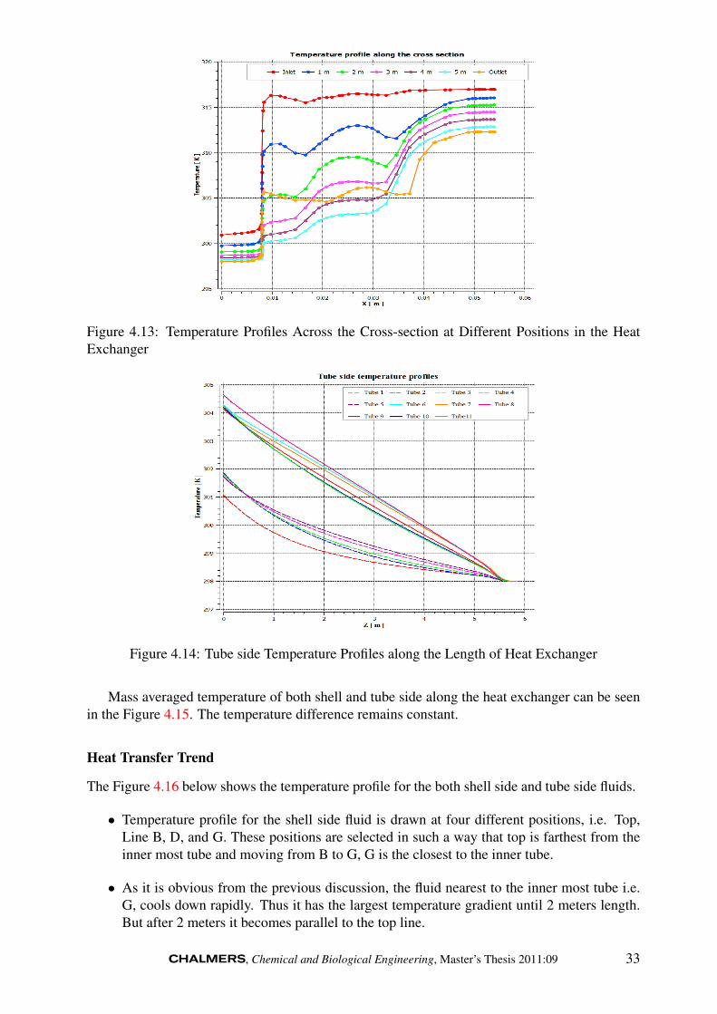
Figure 4.13: Temperature Profiles Across the Cross-section at Different Positions in the HeatExchanger

Figure 4.14: Tube side Temperature Profiles along the Length of Heat Exchanger

Mass averaged temperature of both shell and tube side along the heat exchanger can be seenin the Figure 4.15. The temperature difference remains constant.

Heat Transfer Trend

The Figure 4.16 below shows the temperature profile for the both shell side and tube side fluids.

• Temperature profile for the shell side fluid is drawn at four different positions, i.e. Top,Line B, D, and G. These positions are selected in such a way that top is farthest from theinner most tube and moving from B to G, G is the closest to the inner tube.

• As it is obvious from the previous discussion, the fluid nearest to the inner most tube i.e.G, cools down rapidly. Thus it has the largest temperature gradient until 2 meters length.But after 2 meters it becomes parallel to the top line.


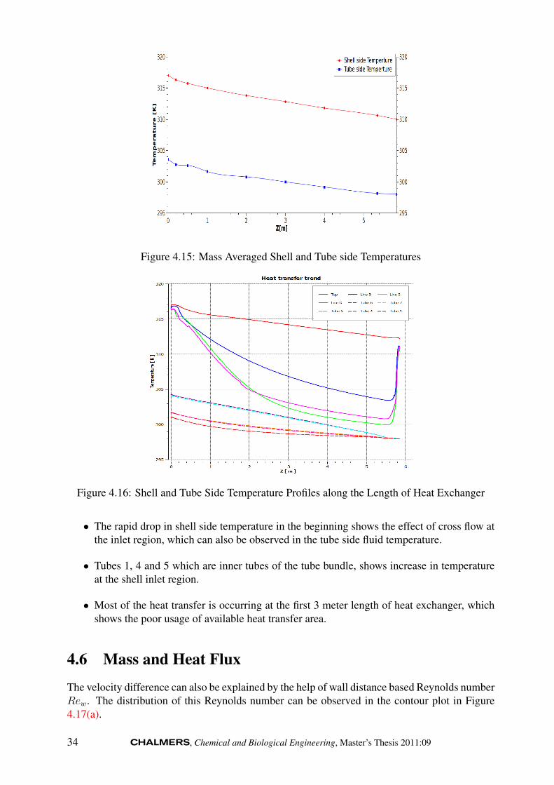
Figure 4.15: Mass Averaged Shell and Tube side Temperatures

Figure 4.16: Shell and Tube Side Temperature Profiles along the Length of Heat Exchanger

• The rapid drop in shell side temperature in the beginning shows the effect of cross flow atthe inlet region, which can also be observed in the tube side fluid temperature.

• Tubes 1, 4 and 5 which are inner tubes of the tube bundle, shows increase in temperatureat the shell inlet region.

• Most of the heat transfer is occurring at the first 3 meter length of heat exchanger, whichshows the poor usage of available heat transfer area.

4.6 Mass and Heat Flux

The velocity difference can also be explained by the help of wall distance based Reynolds numberRew. The distribution of this Reynolds number can be observed in the contour plot in Figure4.17(a).


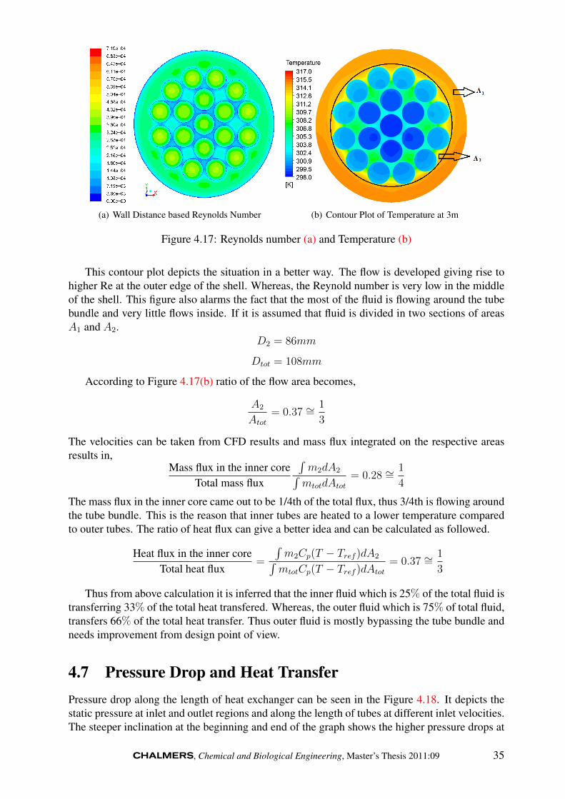
(a) Wall Distance based Reynolds Number (b) Contour Plot of Temperature at 3m

Figure 4.17: Reynolds number (a) and Temperature (b)

This contour plot depicts the situation in a better way. The flow is developed giving rise tohigher Re at the outer edge of the shell. Whereas, the Reynold number is very low in the middleof the shell. This figure also alarms the fact that the most of the fluid is flowing around the tubebundle and very little flows inside. If it is assumed that fluid is divided in two sections of areasA1 and A2.

D2 = 86mm

Dtot = 108mm

According to Figure 4.17(b) ratio of the flow area becomes,

A2

Atot= 0.37 ∼=

1

3

The velocities can be taken from CFD results and mass flux integrated on the respective areasresults in,

Mass flux in the inner coreTotal mass flux

∫m2dA2∫mtotdAtot

= 0.28 ∼=1

4

The mass flux in the inner core came out to be 1/4th of the total flux, thus 3/4th is flowing aroundthe tube bundle. This is the reason that inner tubes are heated to a lower temperature comparedto outer tubes. The ratio of heat flux can give a better idea and can be calculated as followed.

Heat flux in the inner coreTotal heat flux

=

∫m2Cp(T − Tref )dA2∫mtotCp(T − Tref )dAtot

= 0.37 ∼=1

3

Thus from above calculation it is inferred that the inner fluid which is 25% of the total fluid istransferring 33% of the total heat transfered. Whereas, the outer fluid which is 75% of total fluid,transfers 66% of the total heat transfer. Thus outer fluid is mostly bypassing the tube bundle andneeds improvement from design point of view.

4.7 Pressure Drop and Heat TransferPressure drop along the length of heat exchanger can be seen in the Figure 4.18. It depicts thestatic pressure at inlet and outlet regions and along the length of tubes at different inlet velocities.The steeper inclination at the beginning and end of the graph shows the higher pressure drops at


inlet and outlet regions. As described earlier, this happens due to cross-flow and impingement ofthe flow at inlet and outlet of the heat exchanger. Subsequently, heat transfer at these regions ishigher as compared to the rest of heat exchanger. It can be seen in the Figure 4.19 that local heattransfer coefficient is very high at the inlet. This is due to several reasons, mainly being the crossflow at inlet. In addition, the temperature difference between the shell side and tube side fluid ismuch higher as observed in Figure 4.16.

The study of both Figures 4.18 and 4.19 gives an idea of effect of cross-flow over the pressuredrop and heat transfer. Certainly, creating cross-flow regions enhances the heat transfer at thecost of higher pressure drop. Thus it provides an insight about installing baffles for higher heattransfer in this thin and long heat exchanger.

Figure 4.18: Shell Side Pressure Drop along the Length of Heat Exchanger

Figure 4.19: Heat Transfer Coefficient along the Length of Heat Exchanger


Chapter 5

Conclusions

The heat transfer and flow distribution is discussed in detail and proposed model is comparedwith the experimental results as well. The model predicts the heat transfer and pressure dropwith an average error of 20%. Thus the model still can be improved. The assumption of planesymmetry works well for most of the length of heat exchanger except the outlet and inlet regionswhere the rapid mixing and change in flow direction takes place. Thus improvement is expectedif complete geometry is modeled. Moreover, SST k − ω model has provided the reliable resultsgiven the y+ limitations, but this model over predicts the turbulence in regions with large normalstrain (i.e. stagnation region at at inlet of the shell). Thus the modeling can also be improved byusing Reynold Stress Models, but with higher computational costs. Furthermore, the enhancedwall functions are not used in this project due to convergence issues, but they can be very usefulwith k − ε models.

The heat transfer is found to be poor because the most of the shell side fluid by-passes thetube bundle without interaction. Thus the design can be modified in order to achieve the betterheat transfer in two ways. Either, the shell diameter is reduced to keep the outer fluid mass fluxlower or tube spacing can be increased to enhance the inner fluid mass flux. Just doing this mightnot be enough, because it is seen that the shell side fluid after 3m doesn’t transfer heat efficiently.It is because the heat transfer area is not utilized efficiently. Thus the design can further beimproved by creating cross-flow regions in such a way that flow doesn’t remain parallel to thetubes. It will allow the outer shell fluid to mix with the inner shell fluid and will automaticallyincrease the heat transfer.

37

Bibliography

[1] “A heat exchanger applications general.” http://www.engineersedge.com/heat_exchanger/heat_exchanger_application.htm, 2011.

[2] S. Kakac and H. Liu, “Heat exchangers: Selection, rating, and thermal performance,” 1998.

[3] http://www.wcr-regasketing.com, “Heat exchanger applications.” http://www.wcr-regasketing.com/heat-exchanger-applications.htm, 2010.

[4] D. Kern, Process Heat Transfer. McGraw-Hill, 1950.

[5] R. Serth, Process Heat Transfer, Principles and Applications. Elsevier Science and Tech-nology Books,.

[6] E. Ozden and I. Tari, “Shell side cfd analysis of a small shell-and-tube heat exchanger,”Energy Conversion and Management, vol. 51, no. 5, pp. 1004 – 1014, 2010.

[7] J. J. Gay B, Mackley NV, “Shell-side heat transfer in baffled cylindrical shell and tubeexchangers- an electrochemical mass transfer modelling technique,” Int J Heat Mass Trans-fer, vol. 19, pp. 995–1002, 1976.

[8] G. V. Gaddis ES, “Pressure drop on the shell side of shell-and-tube heat exchangers withsegmental baffles,” Chem Eng Process, vol. 36, pp. 149–59, 1997.

[9] F. E. Idelchik, I.E., Handbook of hydraulic resistance. Hemisphere Publishing,New York,NY, second ed., 1986.

[10] M. J. Van Der Vyver H, Dirker J, “Validation of a cfd model of a three dimensional tube-in-tube heat exchanger.,” 2003.

[11] S. B., “Computational heat transfer in heat exchangers,” Heat Transfer Eng, pp. 24:895–7,2007.

[12] A. M. Prithiviraj M, “Shell and tube heat exchangers. part 1: foundation and fluid mechan-ics,” Heat Transfer, p. 33:799–816., 1998.

[13] K. T. C. S. Sha WT, Yang CI, “Multidimensional numerical modeling of heat exchangers.,”Heat Transfer, vol. 104, pp. 417–25, 1982.

[14] N. B. M. Bhutta, M.A.A Hayat, “Cfd applications in various heat exchangers design: Areview,” Applied Thermal Engineering, vol. 32, pp. 1–12, 2011.

[15] J. G. Jae-Young, K. Afshin, “Comparison of near-wall treatment methods for high reynoldsnumber backward-facing step flow,” Int. J Computational Fluid Dynamics, vol. 19, 2005.

[16] E. Cao, Heat Transfer in Process Engineering. McGraw Hill, 2009.

38

http://www.engineersedge.com/heat_exchanger/heat_exchanger_application.htm

http://www.engineersedge.com/heat_exchanger/heat_exchanger_application.htm

http://www.wcr-regasketing.com

http://www.wcr-regasketing.com/heat-exchanger-applications.htm

http://www.wcr-regasketing.com/heat-exchanger-applications.htm

[17] B. Andersson, R. Andersson, L. Hakansson, M. Mortensen, R. Sudiyo, and B. V. Wachem,Computational Fluid Dynamics for Chemical Engineers. sixth ed., 2010.

[18] H. K. Versteeg and M. W., An Introduction to Computational Fluid Dynamics, The FiniteVolume Method. Pearson Education Limited, 2007.

[19] “Ansys fluent theory guide.” http://www.ansys.com, 2010.

[20] “Cfd-online wiki.” http://http://www.cfd-online.com/Wiki/Main_Page,2011.


http://www.ansys.com

http://http://www.cfd-online.com/Wiki/Main_Page

Documents

Heat Transfer Optimization of Shell-and-Tube Heat ...publications.lib.chalmers.se/records/fulltext/155992.pdf · Heat Transfer Optimization of Shell-and-Tube Heat Exchanger through