Embed Size (px)
Citation preview

2013 95
Irene Bolea Agüero
Heat transfer in oxy-fuelfluidized bed boilers
Departamento
Director/es
Instituto Universitario de Investigación MixtoCIRCE
Romeo Giménez, Luis Miguel
Director/es
Tesis Doctoral
Autor
Repositorio de la Universidad de Zaragoza – Zaguan http://zaguan.unizar.es
UNIVERSIDAD DE ZARAGOZA

Departamento
Director/es
Irene Bolea Agüero
HEAT TRANSFER IN OXY-FUELFLUIDIZED BED BOILERS
Director/es
Instituto Universitario de Investigación Mixto CIRCE
Romeo Giménez, Luis Miguel
Tesis Doctoral
Autor
2013
Repositorio de la Universidad de Zaragoza – Zaguan http://zaguan.unizar.es
UNIVERSIDAD DE ZARAGOZA

Departamento
Director/es
Director/es
Tesis Doctoral
Autor
Repositorio de la Universidad de Zaragoza – Zaguan http://zaguan.unizar.es
UNIVERSIDAD DE ZARAGOZA

HEAT TRANSFER IN OXY-FUEL
FLUIDIZED BED BOILERS
PhD Thesis
Irene Bolea Agüero
Supervised by:
Dr. Luis Miguel Romeo Giménez


From the 19th century, the world has witnessed one of the most spectacular
changes on the way of living along the History. The industrial revolution meant a
drastic development for the economy, the quality of life, and the beginning of the
society as we know it now, a globalized world. The steam generation was the
breakthrough that let machines do double in half time than humans. And the coal
has been the element accompanying men on such travel, followed later by the oil
and the gas. But this story of success and progress had also hidden sides that we
did not want to see until they were almost uncovered. Far from flattening, the
curve of production and consumption has been never-ending exponential. From
then on, manufacturing and transportation, the two pillars of the industrial era,
are completely dependent on those non-infinite fuels. Globalization and progress
meant not the same for every country and inequalities accentuate among them.
And, in spite of this, the consequences of the progress of some will be paid by all.
The climate change will be suffered by all the countries. But it is evident that those
with infrastructure will cope better with the up-coming events. The dad
Development must do his job and assumes his responsibilities. We, researchers are
his tools, to carry out this hard task. Each of us must look for the piece of the
jigsaw that is still not placed, to accelerate the change towards a fairer world and
to lessen the irremediable repercussion of the acts of the teenager Progress that
wanted to be Development.


ACKNOWLEDGEMENTS
First I would like to express my deep gratitude to my supervisor Prof. Luis Miguel
Romeo. Since the very beginning of my career he has been an essential guide of my
formation as professional researcher, not only in the technical issues, but also as a
motivating leader and as a contagious optimistic.
I feel very grateful to Dr. David Pallarès for offering me the possibility of spending
a fruitful and pleasant time in Chalmers University of Technology. Without his
invaluable guidance and his opportune advices, this thesis would not have been
what it is. I would like to acknowledge Prof. Bo Leckner for his helpful comments
and ideas, some of which have been the seeds of parts of this work.
I would like to give special thanks to my team, the Oxicocos, Isabel Guedea and
Carlos Lupiáñez, with whom I learnt much about oxy-fuel combustion in fluidized
beds … but I learnt much more about patience, support, understanding, team-
working and friendship.
Along these years I had the luck to meet exceptional people in CIRCE, always
available to help and assist in whatever I needed. Some of them have become very
good friends, willing to patiently listening to any worry about my projects, or to
share some laughs in front of a beer.
Thanks to my family, for their backing, their confidence, their sensitivity and their
love. Especially to my brother David that is in the beginning of his research career,
I hope to be as encouraging as you have been for me.
Thank you Jose, you are part of this work as much as the words that are written in
it.


i
RESUMEN
A pesar de la estabilización de la demanda de carbón en los países desarrollados, su
papel en el mix energético de las próximas décadas es fundamental todavía. El uso
de carbón como combustible incrementará particularmente en las economías
desarrolladas, como India, o China, donde este combustible es abundante y permite
moderar la dependencia energética de potencias extranjeras. Paralelamente, la
comunidad internacional coincide en la importancia de dirigir esfuerzos hacia
políticas que se comprometan a reducir las emisiones de CO2 a la atmósfera en el
corto período hasta 2015. Se han realizado ya avances considerables con respecto a
la eficiencia energética de las plantas de potencia, lo que conlleva la reducción de
las toneladas de CO2 producidas por KWh. Sin embargo, la disminución de
emisiones globales ha de ser más drástica para amortiguar sus consecuencias. A
este respecto, la captura y almacenamiento de CO2 (CCS, Carbon Capture and
Storage) presentan un potencial de reducción de emisiones de CO2 de fuentes
estacionarias de un 25%, en cuanto se encuentren en un desarrollo comercial.
Las tecnologías CCS se agrupan generalmente en tres grandes grupos: las de post-
combustión (final de tubería), pre-combustión (tratamiento del combustible previo a
la combustión) y oxicombustión (combustión con oxígeno sin presencia de nitrógeno
del aire). La oxicombustión de combustibles sólidos, como la combustión
convencional, puede ser implementada en calderas de combustible pulverizado o en
calderas de lecho fluido (CFB, Circulating Fluidized Beds). Esta última tecnología
exhibe unas características de operación especialmente adecuadas para la
aplicación de la oxicombustión. En primer lugar, la versatilidad de combustibles
que pueden ser utilizados, desde biomasa a diferentes rangos de carbones, o
incluso, residuos, tiene un enorme potencial para ser aplicado en el mix energético
de una manera muy flexible. La temperatura moderada y uniforme en el lecho,
evita por un lado la formación de NOx térmico. Por otro, con la adición de sorbentes
cálcicos, esta temperatura optimiza las reacciones de sulfatación y se minimizan
las emisiones de SO2. Si además se implementa la tecnología de captura de CO2 en
oxicombustión, el resultado se aproximaría por fin al concepto de combustión
limpia de carbón.

ii
El interés de la oxicombustión en lecho fluido ha crecido mucho en la última
década. Existen algunas plantas piloto en el mundo dedicadas a profundizar en
aspectos fundamentales del proceso. La planta más grande de oxicombustión en
lecho fluido se encuentra precisamente en Ponferrada, León, y funciona
exitosamente desde 2011. Es una planta demostrativa de 30 MW térmicos,
exclusivamente dedicada a investigación.
Las implicaciones de la oxicombustión en lechos fluidos a gran escala,
particularmente con altos porcentajes de O2 en la corriente oxidante, solo se pueden
pronosticar por el momento, a través de modelos matemáticos. En el Capítulo 2 de
esta tesis, se ha realizado un modelo unidimensional de un lecho fluido circulante
en oxicombustión de gran tamaño. La primera parte de dicho capítulo se dedica a
revisar los modelos existentes y validados para la combustión con aire. Las mismas
estrategias se han aplicado al modelado de la oxicombustión, dividiendo el modelo
en tres módulos interdependientes entre sí: la fluidodinámica, la combustión y
sulfatación, y la transferencia de calor. La validación real de los modelos de
oxicombustión a gran escala no es posible, ya que no existen plantas reales
operando en estas condiciones. En la literatura existen dos grandes compañías que
han publicado los resultados de sus modelos de oxicombustión en grandes lechos
fluidos. Aunque no es posible encontrar los detalles de dichas simulaciones, sus
resultados se han comparado con los del modelo desarrollado aquí, para comprobar
si el grado en que los resultados del modelo son coherentes y fiables.
Los resultados del modelo de oxicombustión en un lecho fluido de gran tamaño se
han analizado desde tres perspectivas diferentes. Por un lado, los futuros lechos
fluidos en oxicombustión permitirán reducir el tamaño de caldera y, con él, los
costes de capital. A medida que se incrementa la concentración de oxígeno en la
corriente oxidante, el área transversal de la caldera habrá de disminuir, para
obtener velocidades adecuadas de fluidización. Los resultados indican que,
incrementando la concentración de oxígeno hasta un 60%, el tamaño de la caldera
pude reducirse un 66%. En consecuencia, el área disponible para intercambiar
calor en las paredes de la caldera, disminuirá también considerablemente. Para
refrigerar la caldera de manera adecuada, los sólidos recirculados habrán de
incrementarse desde 7.8 kg/m2s, hasta 32.7 kg/m2s. La posibilidad de manipular el
caudal de sólidos arrastrados y recirculados, permite una gran flexibilidad para
trabajar a diferentes potencias de combustible. Por ejemplo, para regular

iii
adecuadamente la temperatura de una caldera con una geometría determinada,
que aumente su potencia de 600 MW a 800 MW, los sólidos recirculados habrán de
incrementar 14.3 kg/m2s. De manera análoga, el incremento de concentración de
oxígeno en la corriente oxidante, permite mayor alimentación del combustible, dado
por la estequiometria. De esta manera, con 40% de oxígeno a la entrada, la
temperatura en la caldera puede regularse con dos estrategias complementarias: o
bien incrementando el caudal de sólidos recirculados, hasta 20.7 kg/m2s y enfriarlos
hasta 720ºC antes de introducirlos de nuevo al lecho; o bien, no modificar dicho
caudal, pero disminuir la temperatura a la que los sólidos son recirculados, hasta
620ºC.
Todo este análisis apunta a un protagonismo particularmente relevante de un
equipo de extracción de calor externo a la caldera, el denominado External Heat
Exchanger, EHE. Estos intercambiadores de calor se usan en ocasiones en las
grandes calderas de lecho fluido circulante de combustión convencional, pero en la
oxicombustión, su uso será esencial e inevitable, para poder controlar las
temperaturas en niveles adecuados.
Los EHEs son, en general, intercambiadores de calor de lecho fluido en régimen
burbujeante. Constan de haces de tubos que los atraviesan transversal o
longitudinalmente. Su uso en calderas de lecho fluido en oxicombustión va a
entrañar dos particularidades que aún no han sido abordadas por ninguna
investigación: la diferente composición del gas de fluidización con respecto a su
funcionamiento con aire y la mayor cantidad de sólidos que habrán de ser enfriados
para conseguir las temperaturas de lecho adecuadas.
Por un lado, la composición del gas con el que será fluidizado el EHE, será
diferente. Convencionalmente se ha tratado de aire. En muchos casos, parte del
oxígeno del aire, permite la combustión de partículas inquemadas que llegan al
EHE desde el ciclón. En el caso de la oxicombustión, el aire no puede ser
introducido en el sistema, ya que el objetivo último es obtener una corriente
concentrada de CO2, y la presencia de N2 contaminaría los gases de salida. El gas
con el que se fluidice el EHE será una extracción de los propios gases de escape,
que estarán compuestos de altas concentraciones de CO2. La transferencia de calor
en lechos fluidos burbujeantes se ha estudiado extensamente a lo largo de las
décadas. El mecanismo fundamental de transferencia de calor en este régimen es el
debido a la conducción transitoria de las partículas cuando contactan con la pared
iv
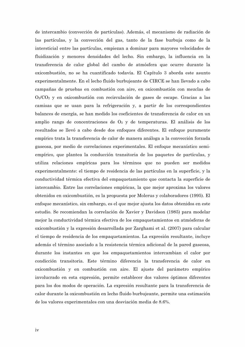
de intercambio (convección de partículas). Además, el mecanismo de radiación de
las partículas, y la convección del gas, tanto de la fase burbuja como de la
intersticial entre las partículas, empiezan a dominar para mayores velocidades de
fluidización y menores densidades del lecho. Sin embargo, la influencia en la
transferencia de calor global del cambo de atmósfera que ocurre durante la
oxicombustión, no se ha cuantificado todavía. El Capítulo 3 aborda este asunto
experimentalmente. En el lecho fluido burbujeante de CIRCE se han llevado a cabo
campañas de pruebas en combustión con aire, en oxicombustión con mezclas de
O2/CO2 y en oxicombustión con recirculación de gases de escape. Gracias a las
camisas que se usan para la refrigeración y, a partir de los correspondientes
balances de energía, se han medido los coeficientes de transferencia de calor en un
amplio rango de concentraciones de O2 y de temperaturas. El análisis de los
resultados se llevó a cabo desde dos enfoques diferentes. El enfoque puramente
empírico trata la transferencia de calor de manera análoga a la convección forzada
gaseosa, por medio de correlaciones experimentales. El enfoque mecanístico semi-
empírico, que plantea la conducción transitoria de los paquetes de partículas, y
utiliza relaciones empíricas para los términos que no pueden ser medidos
experimentalmente: el tiempo de residencia de las partículas en la superficie, y la
conductividad térmica efectiva del empaquetamiento que contacta la superficie de
intercambio. Entre las correlaciones empíricas, la que mejor aproxima los valores
obtenidos en oxicombustión, es la propuesta por Molerus y colaboradores (1995). El
enfoque mecanístico, sin embargo, es el que mejor ajusta los datos obtenidos en este
estudio. Se recomiendan la correlación de Xavier y Davidson (1985) para modelar
mejor la conductividad térmica efectiva de los empaquetamientos en atmósferas de
oxicombustión y la expresión desarrollada por Zarghami et al. (2007) para calcular
el tiempo de residencia de los empaquetamientos. La expresión resultante, incluye
además el término asociado a la resistencia térmica adicional de la pared gaseosa,
durante los instantes en que los empaquetamientos intercambian el calor por
condicción transitoria. Este término diferencia la transferencia de calor en
oxicombustión y en combustión con aire. El ajuste del parámetro empírico
involucrado en esta expresión, permite establecer dos valores óptimos diferentes
para los dos modos de operación. La expresión resultante para la transferencia de
calor durante la oxicombustión en lecho fluido burbujeante, permite una estimación
de los valores experimentales con una desviación media de 8.6%.
v
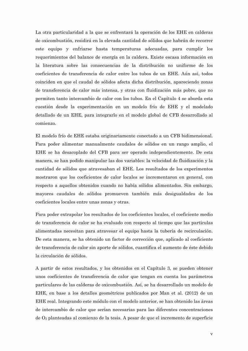
La otra particularidad a la que se enfrentará la operación de los EHE en calderas
de oxicombustión, residirá en la elevada cantidad de sólidos que habrán de recorrer
este equipo y enfriarse hasta temperaturas adecuadas, para cumplir los
requerimientos del balance de energía en la caldera. Existe escasa información en
la literatura sobre las consecuencias de la distribución no uniforme de los
coeficientes de transferencia de calor entre los tubos de un EHE. Aún así, todos
coinciden en que el caudal de sólidos afecta dicha distribución, apareciendo zonas
de transferencia de calor más intensa, y otras con fluidización más pobre, que no
permiten tanto intercambio de calor con los tubos. En el Capítulo 4 se aborda esta
cuestión desde la experimentación en un modelo frío de EHE y el modelado
detallado de un EHE, para integrarlo en el modelo global de CFB desarrollado al
comienzo.
El modelo frío de EHE estaba originariamente conectado a un CFB bidimensional.
Para poder alimentar manualmente caudales de sólidos en un rango amplio, el
EHE se ha desacoplado del CFB para ser operado independientemente. De esta
manera, se han podido manipular las dos variables: la velocidad de fluidización y la
cantidad de sólidos que atravesaban el EHE. Los resultados de los experimentos
mostraron que los coeficientes de calor locales se incrementaron en general, con
respecto a aquellos obtenidos cuando no había sólidos alimentados. Sin embargo,
mayores caudales de sólidos promueven también más desigualdades de los
coeficientes locales entre unas zonas y otras.
Para poder extrapolar los resultados de los coeficientes locales, el coeficiente medio
de transferencia de calor se ha evaluado con respecto al tiempo que las partículas
alimentadas necesitan para atravesar el equipo hasta la tubería de recirculación.
De esta manera, se ha obtenido un factor de corrección que, aplicado al coeficiente
de transferencia de calor sin aporte de sólidos, cuantifica el aumento de éste debido
la circulación de sólidos.
A partir de estos resultados, y los obtenidos en el Capítulo 3, se pueden obtener
unos coeficientes de transferencia de calor que tengan en cuenta los parámetros
particulares de las calderas de oxicombustión. Así, se ha desarrollado un modelo de
EHE, en base a los detalles geométricos publicados por Man et al. (2012) de un
EHE real. Integrando este módulo con el modelo anterior, se han obtenido las áreas
de intercambio de calor que serían necesarias para las diferentes concentraciones
de O2 planteadas al comienzo de la tesis. A pesar de que el incremento de superficie

vi
de intercambio era evidente, dada la cantidad de calor que habría de evacuar el
EHE, este aumento queda moderado por el incremento de coeficiente de
transferencia de calor dado por el mayor caudal de sólidos calientes que atraviesan
el equipo.
Con esta tesis se ha demostrado que las superficies de transferencia de calor en los
lechos fluidos de oxicombustión habrán de adaptarse a las nuevas características
de operación. La relevancia del EHE será particular de los grandes CFB. La
predicción de los coeficientes de transferencia de calor en este equipo diferirá de los
modelos utilizados en la combustión convencional. En consecuencia, para optimizar
el rendimiento de las futuras calderas de oxicombustión en CFB, el diseño de la
configuración del EHE tendrá que tener en cuenta los aspectos tratados en esta
tesis.
CONCLUSIONES
Las grandes calderas de lecho fluido en oxicombustión van a requerir mayor caudal
de sólidos recirculados, para poder moderar la temperatura de manera adecuada.
Esto conllevará un diseño particularizado de los intercambiadores de calor externo
(EHE). Las contribuciones de esta tesis se dirigen a demostrar teórica y
experimentalmente los puntos más diferenciadores en los EHE de un lecho fluido
en oxicombustión de uno en combustión convencional:
- El modelo unidimensional estacionario de lecho fluido circulante (CFB) a
gran escala desarrollado en esta tesis permite cuantificar la evacuación de
calor necesaria en los EHE para las diferentes condiciones de concentración
de O2 en la corriente oxidante y diferentes tamaños de caldera. La
relevancia de este equipo apunta a dos diferencias fundamentales con los
EHE asociados a la combustión convencional: la composición del gas de
fluidización, y el aumento de sólidos recirculados
- El estudio teórico original de los modelos de transferencia de calor en lechos
fluidos burbujeantes, tanto desde el punto de vista empírico como
mecanístico, ayudan a predecir las posibles influencias de los cambios de

vii
composición en las atmósferas de oxicombustión respecto a las de
combustión con aire.
- Los coeficientes de transferencia de calor en el lecho fluido burbujeante de
90 kW se miden y presentan por primera vez en esta tesis durante la
oxicombustión con mezclas de O2/CO2 y con O2 diluido en gases de escape,
para comparar los resultados con los medidos en combustión con aire.
- El tratamiento de los datos experimentales desde los números
adimensionales y desde el enfoque mecanístico, permite proponer una
expresión completa que predice los valores de coeficientes de calor obtenidos
experimentalmente durante la oxicombustión en lecho fluido burbujeante
- La influencia de los sólidos recirculados en la transferencia de calor de un
EHE se analiza experimentalmente en un modelo frío a escala, desacoplado
del CFB original. Los resultados muestran un incremento de la
transferencia de calor con el caudal de sólidos recirculados, a la vez que las
los valores de los coeficientes de calor de unos tubos a otros también
aumentan.
- Por primera vez se propone una expresión que modifique el coeficiente de
transferencia de calor sin recirculación de sólidos, y que tenga en cuenta el
tiempo que tardan las partículas en abandonar el EHE
- La simulación de une EHE, integrado en el modelo de CFB previamente
desarrollado, incluirá el cálculo de los coeficientes de transferencia de calor
tal y como se propone en esta tesis. Este modelo incluirá además el efecto de
la re-carbonatación y sus posibles consecuencias en la de-fluidización del
EHE.
- Finalmente se ha calculado el área de transferencia de calor requerida en el
EHE para diferentes condiciones de concentración de oxígeno a la entrada
del CFB. Gracias a las expresiones desarrolladas aquí, que tienen en cuenta
de manera más realista las condiciones propias de la oxicombustión, las
superficies de transferencia de calor resultantes aumentan a medida que se
incrementa la evacuación de calor necesaria en el EHE, pero de manera más
moderada de lo esperado.

viii

ix
RESUMEN I
CONCLUSIONES VI
NOMENCLATURE XIII
LIST OF FIGURES XIX
LIST OF TABLES XXIII
CHAPTER 1 CONTEXT, JUSTIFICATION AND OBJECTIVES 1
1.1 THE GLOBAL SCENE 1
1.1.1 MAKING THE COAL SUSTAINABLE: THE CO2 CAPTURE AND STORAGE CHAIN
(CCS) 4
1.1.2 STATE OF THE ART OF OXY-FUEL COMBUSTION 9
1.1.3 THE ROLE OF FLUIDIZED BED ON CCS 16
1.2 JUSTIFICATION 17
1.3 OBJECTIVES AND SCOPE 21
CHAPTER 2 LARGE OXY-FUEL CIRCULATING FLUIDIZED BED
BOILER MODELING 25
2.1 INTRODUCTION 25
2.1.1 LARGE CFB MODELING 26
2.1.2 OXY-FUEL CFB MODELING EXPERIENCES 30
2.2 FUNDAMENTALS ON CFB MODELING 32
2.2.1 FLUID-DYNAMICS 35
2.2.2 COMBUSTION AND POLLUTANT FORMATION 39
2.2.3 HEAT TRANSFER 47
2.3 THE OXY-FUEL CFB MODEL 52
2.3.1 FLUID-DYNAMICS SIMULATION 55
2.3.2 COMBUSTION SIMULATION 58
2.3.3 ENERGY BALANCE 64
x
2.4 MODEL VALIDATION 68
2.4.1 AIR FIRING 68
2.4.2 OXY-FIRING 70
2.5 THE ROLE OF THE EXTERNAL HEAT EXCHANGER 74
2.5.1 REDUCTION OF OXY-FUEL BOILER SIZE 74
2.5.2 VARYING POWER INPUT 75
2.5.3 VARYING O2 AT INLET 77
2.6 CONCLUSIONS 79
CHAPTER 3 HEAT TRANSFER IN CIRCE EXPERIMENTAL OXY-FUEL
COMBUSTION BUBBLING FLUIDIZED BED 81
3.1 INTRODUCTION 81
3.2 HEAT TRANSFER IN FLUIDIZED BEDS 82
3.2.1 PREVIOUS FINDINGS 82
3.2.2 THEORETICAL INFLUENCES OF OXY-FUEL CONDITIONS 95
3.2.3 SUMMARY 103
3.3 EXPERIMENTAL SET-UP 104
3.3.1 PREVIOUS EXPERIENCES ON OXY-FUEL FLUIDIZED BEDS PILOT PLANTS. 104
3.3.2 CIRCE OXY-FUEL BUBBLING FLUIDIZED BED PILOT PLANT 106
3.3.3 EXPERIMENTS PLANNING 109
3.4 HEAT TRANSFER COEFFICIENTS MEASUREMENT 113
3.4.1 MEASURING PROCESS 113
3.4.2 HEAT TRANSFER RESULTS 118
3.4.3 UNCERTANITY ANALYSIS 120
3.5 DISCUSSION ON THE RESULTS OF THE HEAT TRANSFER IN OXY-
FUEL BFB 122
3.5.1 EMPIRICAL APPROACH ANALYSIS 122
3.5.2 CONTRIBUTION OF RADIATION HEAT TRANSFER 129
3.5.3 MECHANISTIC APPROACH AND PROPOSAL OF MODIFICATION FOR OXY-FUEL
CONDITIONS 130
3.6 CONCLUSIONS 134

xi
CHAPTER 4 THE INFLUCENCE OF SOLIDS RECIRCULATION ON HEAT
TRANSFER IN AN EXTERNAL HEAT EXCHANGER 137
4.1 INTRODUCTION 137
4.2 HEAT TRANSFER IN EXTERNAL HEAT EXCHANGER FLUIDIZED
BEDS 138
4.2.1 HEAT TRANSFER TO TUBES BUNDLES 138
4.2.2 INFLUENCE OF SOLIDS RECIRCULATION 141
4.2.3 REAL EXTERNAL HEAT EXCHANGERS 145
4.3 EXPERIMENTAL SET-UP 148
4.4 RESULTS OF HEAT TRANSFER IN THE COLD EHE 151
4.4.1 COOLING RATES 151
4.4.2 UNEVEN DISTRIBUTION OF HEAT TRANSFER COEFFICIENTS 155
4.4.3 AVERAGE HEAT TRANSFER COEFFICIENT 158
4.5 INTEGRATION OF THE EHE MODEL IN THE OXY-FUEL CFB MODEL
161
4.5.1 FLY-ASH RE-CARBONATION 161
4.5.2 EXTERNAL HEAT EXCHANGER SIMULATION 167
4.5.3 INTEGRATION RESULTS 169
4.6 CONCLUSIONS 173
CHAPTER 5 SYNTHESIS, CONTRIBUTIONS AND RECOMMENDATIONS
175
5.1 SYNTHESIS 175
5.2 CONTRIBUTIONS 179
5.3 RECOMMENDATIONS AND FURTHER WORK 182
5.4 PUBLICATIONS 183
REFERENCES 187

xii

xiii
NOMENCLATURE
A area m2
A0 gas-distributor area per nozzle m2
BFB Bubbling Fluidized Bed
C molar concentration of a gas compound kmol/ m3
CFB Circulating Fluidized Bed
CCS Carbon Capture and Storage
cp specific heat capacity J/kgK
d diameter m
D bed diameter m
Dg diffusivity of oxygen in nitrogen m2/s
Dsh horizontal dispression coefficient m2/s
Dsv horizontal dispression coefficient m2/s
E enthalpy J/kgK
EHE External Heat Exchanger
f fraction of time of a phase conctacitng a suface
g gravity constant m/s2
Gs elutriated solids mass flux kg/m2s
H bed height m
h heat transfer coefficient W/m2K
HT Heat Transfer
k conductivity W/mK
xiv
kbm backmixing parameter
Kc apparent kinetic constant for surface reaction m/s
kD calcination kinetic constant m/s
l characteristic length scale m
L length m
LHV Low Heating Value kJ/kg
LS loop seal
m mass flow rate kg/s
M dimensionless parameter for the film thermal resistance estimation
n number of
p proportion of particle types -
P pressure bar
Pp partial pressure bar
Q heat kW
r radius m/s
R thermal resistance m2K/W
Rc calcination rate
RFG Recycled Flue Gas
s path length m
S2 typical deviation
T temperature ºC
T average temperature ºC
t time s
tce contact time of clusters in the emulsion
xv
tδ wall thickness m
te emulsion contact time s
tpc contact time of particles attached to bubble
tR time for recycled particles to cross the EHE
u fluidizing velocity m/s
u average velocity
U uncertainty
UA Overall heat transfer coefficient times heat transfer area W/m2
V measured water volumetric flow m3/h
VCu volume of copper m3
VW volume of water m3
xcc carbon fraction in the core
z height above distributor m
Greek Symbols
α thermal diffusivity m2/s
δ volume fraction
∆P pressure drop bar
∆Tln mean temperature logarithmic ºC
ε void fraction
εr radiative emissivity -
εf fouling coefficient m2/W
sφ particle sphericity
η efficiency
Н dimensionless heat transfer coefficient

xvi
κ absorption coefficient 1/m
ν coefficient of kinematic viscosity for flue gas m2/s
ξ a ratio of solids that effectively exchanged heat in the EHE
ρ density kg/m3
σ Bolzman constant m2kg/s2K
τ residence time s
Θ dimensionless time
Ψ dimensionless visible bubble flow
Subscripts
ave average
b bubble
B bed
bb bottom bed
br bubble rising
c cluster
conv convection
d dense phase
disp,h height of disperse phase
e emulsion
eq equivalent
eff effective
f fluidizing/fluidized
g gas

xvii
gc gaseous convection
HT heat transfer
i cell or tube numbering
in instantantaneous
lat lateral flow
m number of measurements
mf minimum fluidization
Pa packet
p particle
pc particle convection
r radiation
ref riser height interval from 0.135 to 1.635 m above gas distributor
RS recycled solids
s solids
sat saturation value
tf throughflow
t terminal
vis visible flow
VOL volatile matter
w wall/wakes
Non-dimensional groups
Ar Archimedes
2gpg
3p
μ
ρρρgd
Fo Fourier Modulus 2l
Dt

xviii
Nu Nusselt g
p
k
hd
Pr Prandtl g
pp,
k
μc
Re Reynolds μ
udρ pg
Sh Sherwood D
kl

xix
LIST OF FIGURES
Figure 1.1. Shares of anthropogenic greenhouse-gas emissions in Annex I countries, 2009,
adapted from IEA (2011a). .................................................................................................. 2
Figure 1.2. World CO2 emissions by fuel. Adapted from IEA (2011a) ...................................... 3
Figure 1.3. CO2 emissions by fuel and sector. Data taken from IEA (2011a) .......................... 4
Figure 1.4. CCS chain scheme .................................................................................................... 5
Figure 1.5. Pre-combustion capture scheme .............................................................................. 6
Figure 1.6. Post-combustion capture scheme ............................................................................. 7
Figure 1.7. Oxy-fuel combustion capture scheme ...................................................................... 9
Figure 2.1. Types of CFB modeling, highlighted the one followed in the current work ....... 26
Figure 2.2. Interaction between the three great groups of phenomena occurring in a CFB
combustor. Adapted from Pallarès and Johnsson (2006) ................................................ 32
Figure 2.3. Dependence of calcination rate on partial pressure and temperature ................ 43
Figure 2.4. Main conversion paths of fuel nitrogen. Adapted from Leckner (1997) ............. 46
Figure 2.5. Dependence of the a) total and b) radiative heat transfer coefficient with the bed
density according to Beritholtz and Leckner (1997) and Krzywansky et al. (2010b) for
different radiating layer thickness, s ................................................................................ 51
Figure 2.6. CFB model flow-chart ............................................................................................. 53
Figure 2.7. CFB boiler mass and energy balance scheme ....................................................... 54
Figure 2.8. CFB fluid-dynamics modeling flow-chart .............................................................. 56
Figure 2.9. CFB combustion modeling flow-chart ................................................................... 59
Figure 2.10. Simulations results of non-convergence of applying volatile composition
methodology, considering. a) CO2, CO, H2, H2O and CH4; b) CO2, CO, H2, H2O, CH4 and
C6H6 .................................................................................................................................... 61
Figure 2.11. Scheme of applying back-mixing parameter, kbm. Z being the char in each cell
............................................................................................................................................. 63
Figure 2.12. Sankey diagram of the CFB ................................................................................. 64
Figure 2.13. CFB energy balance modeling flow-chart ........................................................... 65
Figure 2.14. Energy balance scheme in the dense zone of the CFB ....................................... 66
Figure 2.15. Energy balance scheme in a cell of the dilute zone of the CF ............................ 67
Figure 2.16. Comparison of model pressure profile prediction with the one reported in Yang
et al. (2005) ......................................................................................................................... 68
Figure 2.17. Comparison of flue gas composition prediction with the one reported in Lee
and Kim (1999) ................................................................................................................... 69
xx
Figure 2.18. Comparison of the model temperature profile result with the one reported in
Hannaes et al. (1995) ......................................................................................................... 70
Figure 2.19. Heat transfer share comparison of simulated results with those obtained by
Seddighi et al. (2010) ......................................................................................................... 71
Figure 2.20. Heat duties share model results compared with heat duties estimated by
Saastamoinen et al. (2006) and Nsakala et al (2004) ...................................................... 73
Figure 2.21. Heat transfer share for different oxygen concentration, 650 MW power input 75
Figure 2.22. Heat transfer share for three fuel inputs and same boiler geometry ................ 76
Figure 2.23. Heat transfer share with air design boiler geometry and different O2
concentrations at inlet ....................................................................................................... 78
Figure 3.1. Effect of Reynolds on Nusselt number prediction by different authors .............. 86
Figure 3.2. Dependence of Nusselt number with Reynolds number for vertical tubes
immersed in 500 μm silica sand fluidized bed (Mathur et al., 1986) ............................. 86
Figure 3.3. Temperature effect on effective thermal conductivity ......................................... 90
Figure 3.4. Predicted residence time dependence on fluidizing velocity, by different authors
............................................................................................................................................. 93
Figure 3.5. Gas properties variation for different O2 concentration at inlet: a) density; b)
viscosity; c) conductivity; d) specific heat capacity .......................................................... 95
Figure 3.6. a) Variation of fluidizing velocity, uf, with O2 content in the gas mixture
(constant molar rate of O2) and b) the variation of the total gas molar rate ................. 96
Figure 3.7. Variation of non-dimensional parameters with O2 content in the gas mixture a)
densities ratio, b) Archimedes number, c) Prandtl number ............................................ 98
Figure 3.8. Variation of Reynolds number with O2 content in the gas mixture: a) for a molar
O2 rate b) for constant uf = 1 m/s .................................................................................... 100
Figure 3.9. Effect of O2 content in the gas mixture on Nusselt number predicted by different
authors .............................................................................................................................. 101
Figure 3.10. Prediction of heat transfer coefficient by the Zabrodsky expression (Eq. 3.2)
........................................................................................................................................... 101
Figure 3.11. Emissivity of a gas mixture of CO2 and H2O .................................................... 102
Figure 3.12. Pilot plant scheme: 1- Bubbling fluidized bed. 2-O2 supply bottles. 3-CO2
supply bottles. 4-Propane burner pre-heater. 5- Cyclone. 6-Flue gas heat recovery
exchanger. 7-Bag filter. 8-Induce draft fan. 9-Forced or recirculation draft fan. 10-
Cooling water pump. 11-Air-Water cooler ...................................................................... 107
Figure 3.13. Photo of the fluidized bed pilot plant ................................................................ 107
Figure 3.14. Lower section of the bubbling fluidized bed. Constructive scheme. ................ 109
Figure 3.15. Example of the beginning of the bed cooling (17/02/2011) ............................... 115
Figure 3.16. Fluidized bed heat transfer coefficients measured in each jacket ................... 118
Figure 3.17. Influence of O2 content on non-dimensional parameters ................................. 123
Figure 3.18.Influence of non-dimensional parameters on Nusselt number ......................... 124

xxi
Figure 3.19. Influence of non-dimensional parameters on Nusselt number for similar
fluidizing velocities .......................................................................................................... 126
Figure 3.20. Influence of non-dimensional parameters on Nusselt number for similar bed
temperature ...................................................................................................................... 127
Figure 3.21. Comparison of tests results with prediction by Molerus correlation .............. 128
Figure 3.22. Estimation of the variation of radiant heat transfer coefficient with bed
temperature ...................................................................................................................... 130
Figure 3.23. Maximum and average deviation of predicted values for different values of M
........................................................................................................................................... 132
Figure 3.24. Validation of calculated heat transfer coefficients ........................................... 133
Figure 4.1. Void fraction around an horizontal tube (Umekawa et al., 1999) ..................... 139
Figure 4.2. Dispersion coefficients calculated for different fluidization velocities and
different tubes arrangements, according to Eq. 4.6 and Eq. 4.7. ................................ 141
Figure 4.3. Results from the heat transfer measurement in a cold model of an External
Heat Exchanger. Adapted from Wang et al. (2003) ....................................................... 143
Figure 4.4. Heat transfer rates at different locations of a loop-seal heat exchanger. Adapted
from Johansson et al. (2006) ........................................................................................... 144
Figure 4.5. Heat transfer coefficients measured in different positions in a real HHE. Data
taken from Wedermann and Werther (1993) ................................................................ 146
Figure 4.6. Heat transfer coefficients measured in one of the chambers of the external heat
exchanger. Data taken from Man et al. (2012). ............................................................. 147
Figure 4.7. Experimental set-up. Filled circles indicate the thermocouples location ......... 149
Figure 4.8. Photo of the loop seal, the instrumented tubes bundle, and the air supply ..... 149
Figure 4.9. Example of cooling curve for a testing tube. Zoom to the first seconds of cooling
to calculate the cooling rate. ............................................................................................ 150
Figure 4.10. Cooling rates at the first row, near the distributor, low velocities .................. 152
Figure 4.11. Comparison between low and higher tubes with two solid rates .................... 153
Figure 4.12. Comparison between low and higher tubes with two aeration velocities ....... 153
Figure 4.13. Comparison of four tests at different row heights ............................................ 154
Figure 4.14. Heat transfer coefficients, a) high velocity and increasing solids rate; b) low
velocity and different solids rate ..................................................................................... 156
Figure 4.15. Heat transfer coefficients with two velocities and solids rate conditions ....... 157
Figure 4.16. Influence of a) solids flow, and b) velocities ratio, on the average heat transfer
coefficient .......................................................................................................................... 158
Figure 4.17. Residence time influence on the average heat transfer coefficients ............... 159
Figure 4.18. Influence of residence time of recycled particles on heat transfer coefficients in
the cold model and in the real EHE ................................................................................ 160
Figure 4.19. Carbonation-calcination equilibrium ................................................................ 162

xxii
Figure 4.20. Partial pressure and equilibrium pressure of CO2 along the riser, 40% O2 at
inlet ................................................................................................................................... 163
Figure 4.21. Partial pressure and equilibrium pressure of CO2 along the riser, 60% O2 at
inlet ................................................................................................................................... 163
Figure 4.22. Modeling flow chart of the integration of an External Heat Exchanger into the
global CFB model ............................................................................................................. 168
Figure 4.23. Results of recycled solids flow and heat transfer coefficients in the EHE ...... 170
Figure 4.24. Results of heat transfer coefficients with and without recycled solids, and the
calculated heat transfer surface required for the proper heat exchange ..................... 171
Figure 4.25. Heat transfer coefficients estimated by different authors ............................... 172

xxiii
LIST OF TABLES
Table 1.1. Pilot and demonstration plants of oxy-fuel combustion (Spero and Montagner,
2007; Total, 2007; McCauley et al., 2008; Barbucci, 2009; Burchhardt, 2009; Ochs et
al., 2009a; Scheffknecht, 2009; Sturgeon, 2009; Wall et al., 2009; Alvarez et al., 2011;
Spero et al., 2011; Schoenfield and Menendez, 2012) ...................................................... 13
Table 1.2.. Research groups with experimental experiences on oxy-fuel fluidized bed pilot
plant .................................................................................................................................... 20
Table 2.1. Models of fluidized bed combustors ......................................................................... 33
Table 2.2. Nomenclature of Table 2.1 ....................................................................................... 34
Table 2.3. Correlations for estimating bubble velocity ............................................................ 37
Table 2.4. Coal composition used in the simulations .............................................................. 59
Table 3.1. Empirical expressions for the prediction of heat transfer coefficient from fluidized
bed to vertical walls ........................................................................................................... 85
Table 3.2. Effective thermal conductivity of particulate phase by different authors ............ 90
Table 3.3. Composition of fuels used in the tests ................................................................... 111
Table 3.4. Experiments planning matrix, planned and achieved ranges ............................. 111
Table 3.5. Experimental operational ranges and devices ..................................................... 112
Table 3.6. Summary of AF tests stable zones for heat transfer measurements .................. 116
Table 3.7. Summary of OF tests stable zones for heat transfer measurements .................. 117
Table 3.8. Summary of OF+RFG tests stable zones for heat transfer measurements ........ 118
Table 3.9. Instantaneous and averaging relative uncertainty for heat transfer
determination ................................................................................................................... 121
Table 4.1. Experiments planning matrix for the operation of the cold EHE ....................... 151
Table 4.2. Recarbonation inputs for the simulations ............................................................ 164
Table 4.3. Recarbonation results from the simulations ....................................................... 165


1
CHAPTER 1
CONTEXT, JUSTIFICATION AND
OBJECTIVES
1.1 THE GLOBAL SCENE
In 1992, the United Nations Framework Convention on Climate Change
(UNFCCC) set an intergovernmental framework aimed to be a starting point to
cope with the global climate change. The ultimate objective of the Convention was
“to stabilize greenhouse gas concentrations at a level that will prevent dangerous
human interference with the climate system” (UNFCC, 1992). With 194 Parties, the
UNFCCC has near universal membership. Under the Convention, membership
governments committed to: i) gather and share information on greenhouse gas
emissions, national policies and best practices; ii) launch national strategies for
addressing greenhouse gas emissions and adapting to expected impacts, including
the provision of financial and technological support to developing countries; and
iii) cooperate in preparing for adaptation to the impacts of climate change. This
Convention represented the universal acceptation that human activities are the
major cause of the increasing greenhouse gas emissions in the atmosphere and the
agreement of reinforcing the countries to cope with climate change in cooperation
with the international community. The Parties agreed to take precautionary
measures to anticipate, prevent or minimize the causes of climate change and
mitigate its adverse effects.
The International Panel of Climate Change (IPCC) has been making an
outstanding task of preparing a comprehensive review and recommendations with
respect to the state of knowledge of the science of climate change; social and
economic impact of climate change, possible response strategies and elements for
inclusion in a possible future international convention on climate (IPCC, 2010). In
spite of the international community commitment, facts of greenhouse gas (GHG)

1.1. The global scene
2
emissions to the atmosphere in the last two decades are not as comforting as they
should. According to the Fourth Assessment report by IPCC (2007): ”… the
atmospheric concentrations of long-lived GHGs CO2 and CH4 in 2005 exceed by far
the natural range over the last 650,000 years. Global increases in CO2
concentrations are due primarily to fossil fuel use, with land-use change providing
another significant but smaller contribution.…”. IPCC concluded that reductions of
at least 50% in global CO2 emissions compared to 2000 levels will need to be
achieved by 2050 to limit the long-term global average temperature rise to 2-2.4ºC
(IEA, 2010a).
Energy production is the human activity that represents the major source of CO2
emissions in the developed countries, because CO2 is an intrinsic waste from the
combustion of fossil fuels for power generation.
Figure 1.1. Shares of anthropogenic greenhouse-gas emissions in Annex I countries, 2009, adapted from IEA (2011a).
The economic growth, together with the increasing world population are narrowly
related to the emissions of GHGs to the atmosphere, due to the dependence on the
fossil fuel combustion as primary energy all over the world, in the so-called carbon-
based economy. In spite of the smoother increment of the global GDP, the
international indicators remain unaltered. The small variation of advanced
economies does not alter the global tendency. The rate of growth of OCDE
countries is estimated on 2% in the following 30 years, and the non-OCDE will
grow more than 4.5% (ExxonMobil, 2012). Estimations of the world energy demand
ranged from 30-40% in the following decades (BP, 2011a; ExxonMobil, 2012), while
this growth will achieve 63% in a “usual as business” scenario (EIA, 2011).
CO2; 92%CH4; 7%N2O; 1%
Waste3%
Agriculture8%
Energy83%
Industry6%

Chapter 1. Context, Justification and Objectives
3
Fossil fuels accounts for more than 60% of the electricity generation. Coal has been
a key component of the electricity generation mix worldwide. It fuels more than
40% of the world’s electricity, although this share is higher in some areas. In
countries like South Africa, 93% of power comes from coal, in Poland, 92%, in
China, 79%, in India, 69% and in the United States, 49% (IEA, 2010b). In Europe,
the growth of coal demand is being progressively replaced by the gas, but still
accounts for almost 40 % of the power generation share.
The reports coincide to recognize that energy efficiency continues to improve
globally, and at an accelerating rate. The IEA World Energy Outlook (2011b)
remarks the need to achieve an even higher pace of change, with efficiency
improvements accounting for half of the additional reduction in emissions.
In 2009, 43% of CO2 emissions from fuel combustion were produced from coal, 37%
from oil and 20% from gas, Figure 1.2. Growth of these fuels in 2009 was quite
different, reflecting varying trends that are expected to continue in the future.
Global CO2 emissions actually decreased by 0.5 Gt CO2, between 2008 and 2009,
representing a decline of 1.5%. However, trends varied greatly: the emissions of
developed countries decreased, whereas the emissions of developing countries
increased up to 54%.
Figure 1.2. World CO2 emissions by fuel. Adapted from IEA (2011a)

1.1. The global scene
4
Urgent actions are needed for changing the directions of the CO2 emissions trends,
aiming for the long-term target of limiting the global average temperature increase
to 2°C. Some scenarios are pessimistic about the effectiveness of policies to act
quickly enough. And all of them coincide on pointing out the reduction of CO2
emissions from fossil fuel sources as a priority for a real global reduction.
1.1.1 MAKING THE COAL SUSTAINABLE: THE CO2 CAPTURE AND STORAGE CHAIN (CCS)
Electricity and heat generation accounts for more than 60% of the CO2 emissions
derived from coal combustion (Figure 1.3). This represents most of the stationary
power plants. From a technological point of view, this should be a simplification
when applying measures for emissions reduction from the source itself. This CO2
reduction is based on increasing the power plants efficiency and on deploying CO2
capture and storage technologies.
According to the IEA World Energy Outlook (2011b) widespread deployment of
more efficient coal-fired power plants and carbon capture and storage (CCS)
technology could promote the long-term prospects for coal. Therefore, it is
necessary the development of clean fossil fuels power plants. The development of
zero and near zero emissions power plant technologies is gaining importance
worldwide and large demonstration projects are expected in the coming decade for
new plants (IPCC, 2005). But if drastic reductions are requested in the medium
term, it is also necessary to support and deploy technologies that could be able to
capture part of CO2 from existing power plants.
Figure 1.3. CO2 emissions by fuel and sector. Data taken from IEA (2011a)
Coal
Oil
NG
0
5000
10000
15000
20000
25000
30000
35000
All sectors
CO2emissions in 2009
(millions tonnes)
Elect &
Heat
Manuf.
Coal

Chapter 1. Context, Justification and Objectives
5
There are three main approaches to capture CO2 from fossil-fired energy systems:
pre-combustion, post-combustion, oxy-fuel. These technologies have application in
large, stationary carbon emission point sources. However, capture is only one link
in the CCS chain. A CCS system also requires CO2 compression, a means to
transport it and a storage site, as illustrated in Figure 1.4. This means a great
complexity and effort required to successfully remove CO2 from the atmosphere
that goes beyond the carbon capture step.
Figure 1.4. CCS chain scheme
Looking at Figure 1.4, it is clear that much of the barriers found by any CCS
system to be economically feasible will relay on the way that energy requirements
are minimized and integration of the overall power system with CCS chain
components. Following, the technologies considered for capturing CO2 from fossil
fuel combustion in the near and medium term will be explained.
Precombustion capture
In pre-combustion capture, carbon dioxide is separated from a gaseous fuel mixture
under reducing conditions prior to its combustion. The majority of commercially
available pre-combustion CO2 separation technologies rely on the use of liquid
solvents for absorption of CO2 from a gas stream (Kohl and Nielsen, 1997). CO2 is
usually separated by scrubbing with a physical solvent. A simplified diagram is
depicted in Figure 1.5. It involves the conversion of a carbonaceous fuel, such as
natural gas, coal, biomass or oil to a gaseous mixture that primarily consists of H2
and CO, called syngas. The fuel conversion step during gasification or reforming is
endothermic and requires supplementary heating, typically supplied by partial
Power plant
CO2 capture system
CO2
CompressionCO2
Transport
Flue gas with no CO2
Geological Storage
Heat and power
Heat and power
Fuel
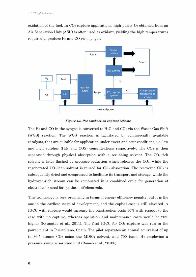
1.1. The global scene
6
oxidation of the fuel. In CO2 capture applications, high-purity O2 obtained from an
Air Separation Unit (ASU) is often used as oxidant, yielding the high temperatures
required to produce H2 and CO-rich syngas.
Figure 1.5. Pre-combustion capture scheme
The H2 and CO in the syngas is converted to H2O and CO2 via the Water-Gas Shift
(WGS) reaction. The WGS reaction is facilitated by commercially available
catalysts, that are suitable for application under sweet and sour conditions, i.e. low
and high sulphur (H2S and COS) concentrations respectively. The CO2 is then
separated through physical absorption with a scrubbing solvent. The CO2-rich
solvent is later flashed by pressure reduction which releases the CO2, while the
regenerated CO2-lean solvent is reused for CO2 absorption. The recovered CO2 is
subsequently dried and compressed to facilitate its transport and storage, while the
hydrogen-rich stream can be combusted in a combined cycle for generation of
electricity or used for synthesis of chemicals.
This technology is very promising in terms of energy efficiency penalty, but it is the
one in the earliest stage of development, and the capital cost is still elevated. A
IGCC with capture would increase the construction costs 30% with respect to the
case with no capture, whereas operation and maintenance costs would be 20%
higher (Kyungtae et al., 2011). The first IGCC for CO2 capture was run in the
power plant in Puertollano, Spain. The pilot separates an annual equivalent of up
to 36.5 ktonne CO2 using the MDEA solvent, and 700 tonne H2 employing a
pressure swing adsorption unit (Romeo et al., 2010b).
GasifierShift CO2 capture
system
Compression, transport and
storage
Heat and power
Power
Fuel
Air
Gas turbine
H2
SyngasCO2
ASU
Steam turbine
N2
Stean

Chapter 1. Context, Justification and Objectives
7
Postcombustion capture
Post-combustion capture refers to the removal of CO2 from flue gases downstream
of fossil-fuelled emission sources. In broad terms, CO2 can be captured using: a)
liquid or solid absorption, b) solid adsorption, and c) membranes. The most mature
post-combustion capture techniques involve liquid absorption using chemical
solvents. Solid-based absorption and adsorption are in the early stages of
development. Membrane technology is somewhat limited in application at the
moment, but the research efforts in this area are significant.
Because post-combustion capture is often implemented in atmospheric air-fired
combustion processes (i.e., low partial CO2 pressure), CO2 is captured by scrubbing
the flue gases with a chemical solvent. Most solvent-based CO2 absorption
processes work in a similar fashion (Figure 1.6): the flue gas is cooled and
channeled to an absorber where it flows counter-current of a chemical solvent.
Most of the CO2 leaves the absorber with the solvent, while the “clean” flue gas
exits at the top. The CO2-rich stream from the absorber is then sent to a stripper
where CO2 is recovered by the application of heat, regenerating the solvent. The
regenerated solvent, also known as the CO2-lean stream, is cooled and recycled to
the absorber. The recovered CO2 is then dehydrated and compressed for transport.
Figure 1.6. Post-combustion capture scheme
Key operational parameters that affect the techno-economics of solvent-based post-
combustion CO2 capture include: flue gas and solvent flow rates, desired CO2
removal, and energy requirements. The flue gas flow rate determines the absorber
BOILER
CO2 capture system
Compression, transport and storage
Flue gas with no CO2
Heat and power
Heat and power
Fuel
Air
Power cycle
Steam
Flue gasCO2

1.1. The global scene
8
size and thus, largely sets the capital costs. The desired CO2 removal affects costs
and energy demands. Higher CO2 recoveries require taller absorbers and incur
higher ancillary energy demands, which are a function of the thermal energy for
solvent regeneration and the electricity for pumps and compressors. The former is
set by the activation energy and reaction kinetics of solvents while the latter is
related to flue gas and solvent flow rates.
Although there are many solvents which can absorb CO2, only a handful of them
have been tested for CO2 capture in post-combustion applications. Aqueous amines
and blends of amines are currently the most suitable solvents, but novel solvents
are under development. Efforts are lately focused on the energy integration of the
capture system into the power plant, in order to reduce the energy penalty
associated with the recovery of the solvent (Romeo et al., 2008).
Oxyfuel combustion
The basic approach of oxy-fuel (OF) combustion is to carry out the combustion
using pure oxygen as oxidant, instead of air. Thereby, the resulted flue gas stream
consists mainly of carbon dioxide and water vapour. The steam is easy to remove
by condensation and so, carbon dioxide is already concentrated for the required
conditioning. Since high temperatures can be reached in the boiler, part of the flue
gas is recycled back into the boiler with the so-called recycled flue gas stream
(RFG). Therefore, it is possible to reach similar conditions of temperature and
volumetric gas fluxes as in air combustion.
Since the oxidant stream contains higher O2 concentration and the diluting CO2 is
denser that the air-N2, the volume of produced flue gas decreases. This means a
reduction in flue gas treatment equipments size and heat losses. This reduction
would be a drawback, if the purpose were the use of sensible heat in the flue gases,
like, in a convective heat exchanger. In Figure 1.7 the blocks diagram of an oxy-fuel
combustion approach is represented.
One of the main advantages that make oxy-fuel combustion a suitable technology
for CO2 capture in power plants is the use of a conventional steam boiler
technology. This is especially attractive when considering retrofit of existing power
plants. However, there are also benefits in applying oxy-firing to new high efficient
power plants, since their increased efficiency reduces the oxygen demand per unit
of generated electricity.

Chapter 1. Context, Justification and Objectives
9
Figure 1.7. Oxy-fuel combustion capture scheme
When operating in oxy-fuel conditions, gaseous species are different. These will
consist mainly of O2, CO2, and water vapour. Density and thermal capacity of gases
and proportion of these compounds differ from conventional air combustion. This
will mean substantial changes in the heat transfer, flame temperature and
stability, combustion efficiency and pollutant emissions. These issues, together
with the high energy requirements of ASU plant, are the main current research
topics in oxy-fuel combustion.
1.1.2 STATE OF THE ART OF OXY-FUEL COMBUSTION
Status
Oxy-fuel (OF) combustion with the purpose of capturing CO2 was first proposed in
1981 and earliest studies were carried out at Argonne National Laboratory (Kiga et
al., 1997; Santos and Haines, 2007). The main reason was its potential for
enhanced oil recovery. However, the oil crisis diminished the interest for CO2
capture. In the late 1990s, attention grew again towards oxy-fuel technology, due to
the imminent necessity of looking for solutions that decrease greenhouse gas
emissions. Differences with the well-known air-combustion (AF) include the heat
transfer mechanism variations, the combustion and ignition processes, the
pollutant formation and the oxygen production technology.
BOILERCompression, transport and
storage
N2
Heat and power
Heat and power
Fuel
Air
Power cycle
Steam
CO2
ASUO2
1.1. The global scene
10
Heat transfer
Radiation heat transfer is the dominant heat transfer mechanism in the furnace of
a conventional pulverized coal boiler. Participative gases, as CO2 and H2O, are
responsible for most of the radiation exchange, emitting, absorbing and scattering
of the energy beams. In studies on retrofit applications, heat transfer show an
increase in the furnace heat transfer but a decrease in the convective pass (Buhre
et al., 2005; Sarofim, 2007; Smart et al., 2009). Convection heat transfer zones,
located normally in cooler parts of the boiler are affected. An increase in the
radiant heat exchange area requires lower temperature difference when passing
through the convective pass. Furthermore, a lower volumetric flue gas flux implies
a lower gas velocity, which also leads to lower convective transfer rates. Payne and
co-workers (Buhre et al., 2005) studied the optimum recirculation rate in order to
reach a heat transfer profile similar to the air-fired combustion system. They
calculated that, with a factor of around 3, this requirement is matched and that, in
the case of fluidized beds, this rate could be smaller, due to better control peak
temperatures by the solids circulation.
In the case of oxy-fuel combustion in fluidized bed boilers attention must be paid
when defining and locating heat transfer surfaces. Since there is less volumetric
gas flows per unit of fuel, boiler size is reduced, but this reduction is limited by the
required fluidization velocity inside the boiler. However, heat transfer surface must
evacuate the same energy than in the air case. This leads to changes in the water
walls design and optimization (Jäntti et al., 2007)
Combustion and ignition
The higher the O2 concentration, the higher inflammability limit and the lower
ignition temperature (Sarofim, 2007). Moreover, flame propagation velocity in
O2/CO2 atmosphere is lower than O2/N2, for the same O2 concentration. In general,
CO2 properties provoke flame instability in the case of using conventional burner
designs. However, this effect could be compensated with oxidant enrichment.
For natural gas and coal combustion, optimum O2 concentration was found to be
between 30% and 35% dry basis, balancing with RFG CO2. However, this optimum
varies depending on the moisture in the fuel, in the RFG and in the ash.
Additionally, O2 partial pressure is higher in oxy-fuel combustion, which allows
reducing O2 excess in the flue gas, while still having a complete burnout.

Chapter 1. Context, Justification and Objectives
11
Regarding oxy-fuel combustion in fluidized bed, the influence of particle size and
lower temperature was recently explored by Guedea et al. (2013). They found
different conversion patterns under O2/N2 and O2/CO2 atmospheres, finding lower
reactivity of char in O2/CO2 mixture, due to lower diffusivity of O2 in CO2.
Emissions control
Pollutant emissions in the case of oxy-fuel combustion highly depend on the
temperature, coal composition and O2/RFG composition. Depending on which
section of the flue gas treatment RFG is taken from, water vapour, SO2, NOx and
other species could be present and these will be fed back to the boiler.
CO2 concentration in the flue gas has reached up to 92% in some pilot scale
experiments. Higher purities were difficult to reach due to air in-leakage into the
boiler (Santos, 2009).
NOx, so as SO2 emissions tend to reduce during oxy-firing, although the
mechanisms of this trend are not yet fully understood. In air-firing case, NOx could
be generated from the nitrogen found in the coal or in the air. Nitrogen from fuel is
the main cause of NOx formation, through a complex chain of reactions. In the case
of NOx from RFG reburning can take place and gets dissociated to form nitrogen.
CANMET research group (Croiset and Thambimuthu, 2001) observed a reduction
of SO2 formation from coal sulphur, compared with air-firing case. SO2 removal has
shown to be enhanced up to 30%, explained by higher kinetics of sulfation of ash,
the inhibition of CaSO4 decomposition in the high SO2 concentrations and a more
porous structure due to high CO2 content in the gas.
SO2 capture in oxy-fuel fluidized bed boilers is generally lower at bed temperature
typical for air-firing, due to changes in the sulfation mechanisms and thus, the
sorbent particle porous structure (de Diego et al., 2011). NOx emissions is, in
general, lower in oxy-fuel fluidized bed boilers, although numerous factors affect its
formation-destruction mechanism, and this issue needs further research (Lupiáñez
et al., 2012).
Oxygen production
Up-scaling oxy-fuel combustion development towards industrial plant sizes
depends mainly on the feasibility of obtaining large quantities of oxygen
economically. Nowadays, there are several technologies for oxygen separation from

1.1. The global scene
12
nitrogen, but only cryogenic is considered feasible for large scale applications. The
largest industrial ASU reported produces 4000t/d, and design studies have been
performed for 7000 t/d, for a single train (Anheden et al., 2005).
Pilot and demo plants
The deployment of oxy-fuel technology involves the whole R&D chain, from basic
research to the technology development. Therefore, the role of the pilot plants and
experimental facilities is rather essential for the acceleration of the
implementation of the CO2 capture technologies.
Five independent main pilot plant studies, carried out by EERC-ANL, IFRF, IHI,
CANMET and B&W-Air Liquid, with furnace sizes ranging from 0.3 to 3 MW,
during late 1980s to 2000s, demonstrated the feasibility of oxy-fuel combustion and
concluded that no technical limitations exist (Santos and Haines, 2005). However,
they recommended further studies for heat transfer issues, especially because of
the differences in temperature distribution along the furnace and the radiation
characteristics.
Two main technologies for coal combustion are applied for large scale power
generation: Pulverized Coal (PC) and Fluidized Bed (FB) boilers. Currently several
industrial scale steam generation plants are projected and some of them are
already in the commissioning phase. In Table 1.1, main pilot and projected
demonstration plants for oxy-firing combustors are gathered.

Chapter 1. Context, Justification and Objectives
13
Project/ Institution
Country Size
(MWth) Status
/Schedule Boiler Type
Fuel CO2
capture dtails
Babcock & Wilcox
USA 30 Demonstration
tests during 2007-2008
Pilot PC Bit.
SubBit, Lig
No Capture
Jupiter USA 15 Start-up 2011 PC retrofit.
No FGR
NG, , High
sulphur coal
25% flue gases to be treated. No
storage Doosan Babcock
UK 40 Start-up 2009 Pilot PC
Vattenfall Germany 30 Start-up 2008 Pilot PC Lig. Bit. With CCS
Total, Lacq France 30 Start-up 2009 Industrial. Steam for utilities
NG and Liq.
Fuels
With CCS in gas
depleted reservoir
Enel Italy 48 Start-up
planned 2012 Presurized
PC
Jupiter (Pearl Plant)
USA 66 Started-up
2009 22 MWe PC Bit Side stream
Callide Australia 90
Air tests in March 2009 O2/CO2 plant
contract: August 2009
30 MWe Retrofit PC
Bit
75 tpd to CCS. Road
transport to a depleted gas field
Ciuden-PC Spain 20 Start-up in
2010
Pilot PC Antr.
Pet cok
Ciuden-CFB
Spain 30 Pilot CFB Antr.
Pet cok
Babcock & Wilcox
USA 400 100 MWe
PC SubBit With CCS
Jamestown USA 150 Announced for
2015
CFB 78 MWe gross /44
MWe with CCS
Bit, biomass
With CCS to Michigan
Basin
Endesa Spain 1500 Announced for
2015 With CCS
Vattenfall Germany 1000 Announced for
2015 250 MWe
PC Lig. Bit. With CCS
KEPCO (Young-dong)
Korea 400 Announced for
2016 100 MWe
Repowering SubBit,
Bit With CCS
Table 1.1. Pilot and demonstration plants of oxy-fuel combustion (Spero and Montagner, 2007; Total, 2007; McCauley et al., 2008; Barbucci, 2009; Burchhardt, 2009; Ochs et al.,
2009a; Scheffknecht, 2009; Sturgeon, 2009; Wall et al., 2009; Alvarez et al., 2011; Spero et al., 2011; Schoenfield and Menendez, 2012)

1.1. The global scene
14
Barriers and future prospects
Large Scale Oxygen production
One of the great drawbacks of oxy-fuel combustion comparing with other CO2
capture technologies is the energy cost of oxygen production. Current technology,
based on cryogenic air separation, for producing 95% purity O2, requires around
200 kWh/tonO2 (Sarofim, 2007). In a steam power plant this means energy losses of
around 7%-10% of the LHV efficiency. Possibilities of achieving higher O2
production efficiency with the current cryogenic ASU are limited. An added
drawback of this technology is the residual N2 that remains in the oxygen stream.
It can reach up to 5% volume diminishing CO2 stream purity. However, different
concepts are also investigated: Ion Transport Membrane (ITM), developed by Air
Products, is a promising technology. It operates at temperatures around 800-900ºC,
at which the crystalline structure incorporates oxygen ion vacancies (White et al.,
2009). Oxygen Transport Membrane (OTM), patented by Praxair, is also a new
technology based on droped Zirconia, being able to consume 75% less power than
cryogenic ASU (Wilsoon et al., 2009). Membranes show the advantage of avoiding
presence of N2 from air, and only bound N2 would be present in the gas stream.
Ceramics Autothermal Recovery (CAR) is under development by Linde and BOC
(Santos, 2009).
CO2 cleaning for disposal
Some research is needed to know the effect of recycling flue gas stream from the
different points of the flue gas circuit: recirculation fans consumption, flue gas
cleaning equipments sizing, or increase in accumulated pollutants in the boiler are
some of the issues under study (Kather, 2007). Flue gas desulphurization tests
were already carried out in Schwarze Pumpe, obtaining similar results as in air-
firing cases (Yan et al., 2009)
On the other hand, uncertainties in the purity requirements for CO2 geological
disposal are still an issue, although some guidelines were determined from ENCAP
project (Sarofim, 2007). In this respect, CO2 stream from oxy-fuel combustion has
more non-condensable species concentration than from other capture technologies
(Seevam et al., 2008). Properties of gasses blends are not known around the critical
point and changes in the phase diagram due to the presence of non-condensable
gases in the CO2 stream are difficult to determine. O2 content in the flue gas

Chapter 1. Context, Justification and Objectives
15
stream is around 3%. This represents a great drawback when the storage site is a
depleted hydrocarbon site, because high probability of combustion reactions. In this
case, O2 should be removed before storage.
Moreover, undesired air ingress into the system is the major source of impurities in
oxy-firing process. These leakages could be reduced by pressurizing gas feeding
into the boiler. Especial care must be taken with NOx, SO2 and O2 content, which
represent around 0.25%, 2.5% and 3% vol. respectively. NO and SO2, can react in
the compressors in the presence of water and oxygen, forming H2SO4 and HNO3.
New concepts are also proposed, for integrating captured CO2 with compression
phase (Romeo et al., 2009a). For diminishing compression costs, pressurized
combustion systems would lead to a high pressure flue gas stream, for example, in
the case of a pressurized fluidized bed. In the case of oxy-fuel, this would also help
to avoid air leakages into the system, reaching a higher purity CO2 stream.
Burners and boilers design
Adjustments in the burner designs need to accomplish several issues: higher
oxygen feed concentration, different primary air for fuel conveying, different
aerodynamics due to denser CO2 gas around the burner and changes in flame
staging because of NOx feeding with RFG. With the help of computational fluid-
dynamics modeling, new burner designs have been proposed by several researchers
from academia and industry (Becher, 2008; Tchunko et al., 2008; Lee et al., 2009;
Scheffknecht et al., 2009; Seltzer et al., 2009)
Regarding the boiler design, heat and energy balances are changing in the case of
oxy-fuel combustion. As explained above, heat transfer is modified by the flue gases
properties and flows. This leads to a re-sizing of the heat transfer exchange areas,
reducing the radiant zone and increasing the area of the convective pass (Jordal et
al., 2004; Jäntti et al., 2007; Ochs et al., 2009b). High ash fuels could also cause
slugging and fouling problems in the radiant area (Scheffknecht, 2009).
Fluidized bed combustors are a highlighted option for implementing oxy-fuel
combustion in the medium term time framework. In general, fluidized bed
technology presents interesting characteristics when compared to pulverized fuel
boilers, mainly related to the pollutant emissions control. This has allowed to
improve the combustion performance of difficult, such as low-rank fuels, or fuels

1.1. The global scene
16
that are difficult to pulverize. Additionally to these known advantages, fluidized
bed present a remarkable feature that makes it suitable for burning under oxy-fuel
conditions. Thanks to the high bulk density of inert particles and their movement,
temperature is easier to control and uniform. For high O2 concentration in
fluidizing streams higher fuel is fed for the same boiler geometry. More compact
boilers lead to less boiler wall surface to exchange heat. Along next section,
fluidized bed combustion fluidized beds will be explored.
1.1.3 THE ROLE OF FLUIDIZED BED ON CCS
The particular characteristics of fluidized bed (FB) technology are caused by the
fluid-like behavior of certain types of solids particles when a liquid or gas suspends
them from below. Such a basic phenomenon provides an intense contact and
interaction between the fluidization substance and particles and among the
particles themselves. This allows FB to be susceptible to be applied to numerous
industrial processes. Energy conversion in all its forms is one of the major
applications for fluidized beds. Initially, fluidized beds were conceived by Fritz
Winkler in 1912 for coke gasification. It was not until the 60’s when Douglas Elliot
recognized the possibility of burning coal in fluidized beds to generate steam (Basu,
2006).
The use of fluidized bed boilers has grown drastically in the last years. One of the
main reasons is that environmental regulations have become stricter regarding
pollutant emissions from combustion sources. Fluidized beds have the capability of
capturing SO2, thanks to the addition of calcium-based sorbents directly to the
furnace. One of the main problems that fluidized bed combustion must cope with is
the risk of inert matter agglomeration. This phenomenon is due to the melting of
solids particles due to peaks of temperature. Melted particles become sticky and
form agglomerates extremely quickly. This drives to a bed defluidization and
consequent un-desirable operation turn off. For avoiding this problem, bed
temperature must be always kept below ashes melting temperature. This is
actually not a real handicap, having into account that optimum temperature for
SO2 capture under conventional air-firing is around 850ºC. Additionally, this
temperature is sufficiently low for avoiding thermal mechanisms of NOx formation,
lowering the emissions of this compound as well.
Chapter 1. Context, Justification and Objectives
17
For these reasons, fluidized bed is a very promising candidate to apply oxy-fuel
combustion as a CCS technology. The support given by the European Commission
to the deployment of oxy-fuel combustion to large circulating fluidized bed boilers,
has been translated into two highly relevant projects within the Seventh
Framework Program. First, the Flexi-Burn project, funded with 6.4 million Euros,
started in 2009 and ended in 2012. Its aim was fully utilizing all the new CFB
design and advancements for merging a CFB boiler with supercritical one through
(OT) steam cycle and air separation unit, together with the CO2 capture unit. The
air/oxy flexible concept aim to have the capability of substituting 20% of the coal
input with biomass fuels. The demonstration phase in this project took place, in
parallel, in the CIUDEN 30 MWth CFB plant, for the oxy-fuel tests, and in Lagisza
plant, the 460 MWe OT CFB boiler.
The second project, called O2GEN, within EU Seventh Framework Program was
approved in the beginning of 2012, with a funding of 6 million euros. It will be
coordinated by CIRCE. The focus is now to optimize and integrate the main
components of the oxy-fuel CO2 capture system, the ASU, the CFB boiler and the
compression unit, aiming to reduce the overall energy penalty down to half of the
current state of the art. The demonstration stage will be mainly developed in the
30 MWth CFB unit in CIUDEN and the results will be deployed in the OXY-CFB-
300 Compostilla Project (Table 1.1). The Compostilla Project was selected by the
European Energy Program for Recovery (EPR) to receive funding of 180 milion
Euros to develop the technology. It will be the first demonstration scale oxy-fuel
power plant, based on supercritical CFB boiler, involving the whole CCS chain.
1.2 JUSTIFICATION
From a global point of view, the research community has an urgent task to develop
instruments for avoiding CO2 emissions to the atmosphere as soon as possible, as
has been internationally recognized. The consequences of the climate change are
imminent, and the necessity of mitigate CO2 emissions from anthropogenic origin
is an issue of absolute priority. One of the most relevant sources of CO2 is the large
fossil fuel combustor used in the energetic and the steel and concrete sectors.
It is clear that avoiding emissions from large stationary sources, such as said
boilers and combustors, the essential contribution CO2 capture and storage

1.2. Justification
18
technologies, has been recognized by the international authorities, as revealed by
the Working group III report for the UNFCC on CO2 mitigation (Sims et al., 2007).
Still, it must be beard in mind, that CCS must be a transition technology towards
the decarbonization of energy sources (IEA, 2011c).
The CCS chain technology acquires especial relevance for the appliance to de-
localize, low-cost and carbon intensive fuels, such as coal. Indeed, coal is the fuel
with the largest R/P ratio (reserves-to-production) and the world proved reserves in
2010 were sufficient to meet 118 years of global production. Moreover, in 2010 the
world coal production grew around 6% over the historical average, and Asia Pacific
region accounted for 89% of global growth. Solely China is planning to build 110
GWe of supercritical power plants by 2015 (BP, 2011b). Additionally given the
successful commissioning of the first supercritical CFBC at Lagisza (Poland), both
China and Russia are initiating programs for constructing supercritical CFBC
units (Burnard and Bhattacharya, 2011).
It is then clear that fluidized bed technology is gaining importance because its
unique features for burning broad range of local solid fuels. Particularly relevant is
its capacity of avoiding SO2 emissions by the addition of limestone based sorbents
inside the boiler, contributing this way to the use of low-rank local lignite,
indigenous of many regions around the world. The possibility of keeping
temperatures, also below the point of NOx thermal generation, drives fluidized bed
combustion process to the concept of clean coal technology approach. It appears
then as an outstanding opportunity for applying oxy-fuel combustion into this type
of technology. This will be the first step towards developing a realistic concept of
zero-emissions coal power plants.
From this perspective, oxy-fuel stands as one of the three feasible technologies to
be implemented in the near term and, in fact, already at the demonstrations stage.
Although the ratio of CFB combustors over the PC combustors for conventional air-
firing was only around one fourth in North America and Europe was in 2007
(Koornneef et al., 2007), the oxy-fuel pilot and demonstration roadmap shows that
both technologies are considered equally suitable. In fact, the two options are
already working at a demonstration scale, 30 MW. Oxy-fuel PC was commissioned
in 2008 in Schwarze Pumpe (Germany) and oxy-fuel CFB began operation in
CIUDEN (Spain) in 2011 (Alvarez et al., 2011).

Chapter 1. Context, Justification and Objectives
19
With this global picture in mind, research must be focused on overcoming the
barriers to make oxy-fuel (OF) technology a reliable option for the new power
plants generation. Expected differences with the well known air-firing (AF)
technology have been early recognized. The main research groups that have carried
out experiments on oxy-fuel pilots plants are summarized in Table 1.2.
As seen in Table 1.2, one of the main concerns of scientific community is coping
with the pollutant emissions inherent in solid fuels combustion, particularly coal.
This is the reason why most of the studies focus on looking deeper inside the SO2
capture and NOx destruction during OF mode. Many of the groups, in fact, had
experiences on the research on these topics and retrofitted existing plants to adapt
them to OF, like in CANMET, Utah or VTT.
From the table it is noteworthy that little attention has been paid to the behavior
of the fluidizing bed itself. It has been widely recognized that the distinguishing
particularities inherent to the fluidized bed technology are related to the movement
of particles, strongly influencing heat transfer inside and thus, providing the
outstanding characteristic of uniform and controlled temperature. Heat transfer
during OF in FB has been only measured by ALSTOM (Nsakala et al., 2004),
finding not remarkable differences between AF and OF heat transfer coefficients,
although no numerical values were published. However, as stated by Eddings et al.
(2009), the control of bed temperature when fixing exit O2 will be critical when
varying oxygen levels.
At great scale, some modeling results have been published, highlighting the role of
a proper recycled solids rate and temperature for a proper control of bed heat
balances (Nsakala et al., 2004; Saastamoinen et al., 2006; Seddighi et al., 2010).
This temperature control will be an issue narrowly related with the SO2 capture
process. On the one hand, as stated by García Labiano et al. (2011) optimum
temperature for SO2 capture will differ from AF conditions, increasing for OF
mode. Also, as indicated by Varonen (2011) or Nsakala et al. (2004), there are high
probability of recarbonation of fly-ash, giving place to problems in the heat
exchanger tubes, or meaning a risk of de-fluidization in the large CFB external
heat exchanger. Additionally, temperature in fluidized beds must be strictly
controlled under the limits of agglomeration and sintering risk.

1.2. Justification
20
Group Experimental
facility Modeling Issues Refs
CANMET CFB
ID 100 mm H= 5 m
No Sulfure Capture NOx emissions
(Jia et al., 2007)
VTT CFB
ID167 mm H=8 m
Yes, dynamic simulation
Sulfure Capture NOx emissions
(Pikkarainen, 2007)
Czestochowa University of Technology
CFB ID 250 mm
H=5 m
Yes, at large scale (not validated)
Fuel conversión (S,N,C)
(Czakiert et al., 2010;
Krzywanski et al., 2010a)
ALSTOM
CFB ID lower = 0.66
m ID upper = 1 m
H = 18 m
Yes, at large scale (not validated)
Sulfure Capture NOx emissions Combustion efficiency
Heat transfer
(Nsakala et al., 2004)
CSIC-ICB BFB
ID 100 mm H = 0.6 m
No Sulfure Capture
(de Diego et al., 2011)
University of Utah
CFB ID 250 mm H = 6.4 m
No Sulfure Capture NOx emissions
(Eddings et al., 2009)
METSO CFB
1 x 1 m2 H = 13 m
Yes Sulfure Capture NOx emissions
(Seddigh et al., 2011; Varonen,
2011)
Wien Technical University
CFB ID 150 mm
H =5 m
No Sulfure Capture NOx emissions CO emissions
(Tondl et al., 2011)
CNR BFB
ID 40 mm H = 1 m
Yes Sulfure Capture Attrition
(Scala et al., 2011)
CIRCE BFB
ID 207 mm H = 2.7 m
Yes
Sulfure Capture NOx emissions CO emissions Combustion efficiency
Fluid-dynamics Heat transfer
(Romeo et al., 2010a;
Guedea et al., 2011;
Lupiáñez et al., 2011)
Table 1.2.. Research groups with experimental experiences on oxy-fuel fluidized bed pilot plant
For this reasons the current research is going to stress the attention on the heat
transfer during the oxy-fuel fluidized bed operation. Results will have to be
extrapolated towards the implications that these results will have on the future

Chapter 1. Context, Justification and Objectives
21
large oxy-fuel boilers. Second generation designs of oxy-fuel boilers working with
higher concentration of O2 in the comburent, will need to handle greater heat
removal with less available surface for this exchange.
1.3 OBJECTIVES AND SCOPE
In spite of the existence of several experimental pilot plants worldwide, running
oxy-fuel experiments, none of them have measured heat transfer during oxy-fuel
combustion in the bubbling zone of a fluidized bed. The relevance of this issue,
resides not only in the quantification of heat transfer during the combustion in an
oxy-fuel boiler. Large oxy-fuel boilers will have to handle greater solids rates and
the overall heat balance of plant will change. The external heat exchangers
attached to the CFB boilers in the solids recycled loop will gain an essential
relevance. These devices work, in most of the cases, in a bubbling regime, to assure
a proper conveying of solids back to the boiler. Heat from recycled hot particles will
be removed partly on this device. It is assumed that the external heat exchanger
will be fluidized with recycled flue gas, consisting mostly on CO2. The conditions in
an external heat exchanger of an oxy-fuel boiler, will be similar to those existing on
our bubbling oxy-fuel fluidized bed. Hence, the study of the heat transfer in the
bubbling fluidized bed under oxy-firing conditions will be essential to correctly
make proper design assumptions in future external heat exchanger devices.
This thesis aims to demonstrate which will be the key aspects that will modify the
heat transfer surfaces design in the future commercial scale oxy-fuel CFB boilers.
With this purpose, this thesis will be addressed to:
establish how the heat balance of a large CFB will change in oxy-fuel
combustion
quantify the heat transfer during oxy-fuel combustion in a bubbling
fluidized bed, under several operating conditions
assess which will be the practical consequences of these changes within the
plant configuration
evaluate the influence of larger solids recirculation on the performance of
the external heat exchanger fluidized beds
By means of a mathematical model of a large-scale oxy-fuel boiler, results will
highlight the relevance that extra heat transfer surfaces to acquire a proper heat

1.3 Objectives and scope
22
balance of the plant when applying oxy-fuel combustion to the boiler. The external
heat exchanger (EHE) will be then an essential device in future oxy-fuel CFB
boilers. A new sub-model of generic EHE will be developed and integrated in the
CFB loop previously developed. The appropriate estimation of the heat transfer
coefficients in the EHE during fluidization with recycled flue gases lead to great
uncertainties to quantify the heat transfer surface needed in the EHE for certain
cooling requirements. Since the conventional frame of operation of EHE are inside
the bubbling regime, measurements of heat transfer in the oxy-fuel bubbling
fluidized bed pilot plant in CIRCE will give useful information. Additionally the
contribution of recycled solids through the EHE on the heat transfer coefficient will
be also quantified, by means of experiments on a EHE cold model. Experimental
derived expression will be then included in the EHE sub-model, to reach the heat
transfer surface area required under several oxy-fuel conditions.
This work is divided into three different sections:
First, a comprehensive one-dimensional model of a large-scale circulating fluidized
bed has been developed. Oxy-fuel conditions have been run in the model. Results of
the energy balance and the main difference of the operation conditions are
explained in Chapter 2. The reader will find a review of the main modeling
approaches and the explanation of the model itself, dividing the overall program in
three main sub-models: fluid-dynamics sub-model, combustion sub-model and heat
transfer sub-model. Validation of the model in air-firing conditions is made against
literature results of large-CFB boilers. The energy balance validation under oxy-
fuel conditions is also compared with three published reports by different authors.
The results are shown, analyzing the consequences of changing O2 content at inlet,
the temperature of recycled solids and the effect of the boiler geometry on the
overall plant balance. An essential role of the external heat exchanger device is
drawn from this study. This will lead to the next section, when heat transfer in an
oxy-fuel bubbling fluidized bed will be studied.
Chapter 3 explores the main previous findings on heat transfer in fluidized beds,
and the expected influence of oxy-fuel conditions, according to the known
approaches. Heat transfer coefficient is then measured during the oxy-firing
operation in the bubbling fluidized bed pilot plant in CIRCE. The bubbling
fluidized bed pilot plant is described, and the way of cooling the bed during
operation is explained. Influences of oxy-fuel conditions on the coefficients are
Chapter 1. Context, Justification and Objectives
23
analyzed and the main parameters affecting heat transfer are determined. Further
discussion is driven under the perspective of fully empirical models, and the
mechanistic semi-empirical approaches. A complete expression for the evaluation of
heat transfer coefficients under oxy-fuel combustion is proposed, fitting the
experimental heat transfer coefficients measured.
In the next section of this work, the experiments carried out on the cold model of a
EHE are explored and discussed. On the one hand, the non-uniformity of local heat
transfer coefficient across the EHE is measured. On the other hand, the average
heat transfer coefficient will allow quantifying the contribution of the solids
recirculation to the heat transfer coefficient when no solids are recycled. The
expression derived from the experiments can be then included in an EHE sub-
model, to be integrated in the overall CFB loop. From a design point of view, the
great differences of heat transfer surface needed for different operational
conditions will be analyzed.
This thesis intends to be an important support for the second generation oxy-fuel
boilers designs. It aims to cover the main implications of the heat transfer on the
plant balance and so, being a breakthrough to reach the optimum boiler efficiency
when working under oxy-fuel conditions.

24

25
CHAPTER 2
LARGE OXY-FUEL CIRCULATING
FLUIDIZED BED BOILER MODELING
2.1 INTRODUCTION
Combustion in fluidized bed has outstanding characteristics that make it
advantageous in some aspects compared to the conventional pulverized combustion
boilers. However, due to the presence of a large amount of particles and the effect
of interactions among them, numerous phenomena take place at the same time.
Thus, in spite of being an acknowledged mature technology, its complexity makes
research efforts be kept addressed towards a better understanding of the processes
taking place inside the boiler for more accurate and less tedious prediction of the
system behavior.
Processes modeling in general and fluidized bed modeling in particular, can level,
at least, at one of the following objectives:
I. to interpret data obtained from experimental plants, like in Redermann et
al. (2009) or
II. to scale-up processes that are already running at lab-scale (Breitholtz. and
B., 2000);
III. to optimize existing systems, like the one developed by Heikkinen et al.
(2009) and
IV. to predict changes in conventional process or operational conditions, as
made by Krywanski et al. (2010a).
This last is the purpose of the present work. The main concern here will be
assessing the effects of oxy-fuel combustion in fluidized beds at large scale. With
this aim, a model is developed, based on the knowledge of conventional air-CFB
combustors. A review of the main modeling strategies for large circulating fluidized

2.1. Introduction
26
boilers will provide us the criteria to select the appropriate modeling approach to
reach adequate results. A one-dimensional steady-state semi-empirical modeling
has been applied then to the current programming. The model predictions will be
first compared with air-firing public data from large plants. Since no oxy-fuel large
scale plants are commercially available yet, results of the current model will be
analogized with three models published. The analysis by means of the current
model will be assesed from two different approaches: i) modification of boiler
geometry, imposing certain operational requirements, from the design point of
view; ii) variation of O2 concentration and fuel input, for the operational
perspective, keeping unchanged the boiler geometry.
The model will highlight the relevance of allocating extra heat transfer surface out
of the conventional water walls, wing walls or convective pass, to properly control
the bed temperature.
2.1.1 LARGE CFB MODELING
Mathematical modeling is an essential tool for predicting operational behavior of
existing plants or analyzing effects on the process when conventional input
parameters are changed. With this purpose, researchers and boiler companies have
been trying to develop different ways of representing CFB performance. Different
approaches can be found depending on the aim of the model itself, Figure 2.1.
Modeling of the system response, when facing changes in the input parameters, is
the focus of the dynamic approach. These models predict the system behavior with
time when fuel load changes (Park and Basu, 1997; Chen and Xiaolong, 2006), or
fresh particles are entering the system (Hartge et al., 2007). Changes on the
comburent composition, like in the transition to oxy-fuel combustion, is being lately
investigated by the group in VTT (Pikkarainen, 2007).
Figure 2.1. Types of CFB modeling, highlighted the one followed in the current work
CFB Modeling
Steady
Semi-empirical CFD
Dynamic

Chapter 2. Large oxy-fuel circulating fluidized bed boiler modeling
27
Major number of models is focused on simulations assuming stable conditions with
time. When considering steady-state simulations, two different types of models can
be used: models based on a semi-empirical approach or models based on
Computational Fluid-Dynamics (CFD). This last approach has been receiving
increasing attention lately, but it must be considered under research, assuring a
mesh, independent sub-grid model (Wang et al., 2010). One of the latest works on
3D CFD modeling of a large-scale CFB was performed by Zhang et al. (2010). They
aimed to reach a virtual simulator of large-scale boilers. They reached a quite good
fit of experimental data with modeling results, but still, complex phenomena such
as mass and heat transfer processes were not included in the model. In
Lappeenranta University the group of Timo Hyppänen is leading the CFD
modeling of the Foster Wheeler 330 MWe Flexi-Burn boilers at large scale
(Myöhänen et al., 2012).
Many researchers, however, bet for compromising accuracy at hydrodynamics
prediction, by using empirical or semi-empirical expressions, with the aim of
including fuel conversion and heat transfer phenomena into the model. Most of
these models adopt a lumped model approach by dividing the boiler in dense and
freeboard zones and, sometimes, sparse zone, dilute zone and exit zone are
considered inside the freeboard as well. These parts are treated differently,
depending on the processes taking place, but relations among them must always be
included.
One of the extended one-dimensional CFB large scale models intended to become
the basis for a common computer code was the one used by the IEA mathematical
modeling group (Hannaes et al., 1995). The aim was to simulate the operation of a
CFB defined by overall geometry, coal and limestone feed rates and composition,
air feed and air staging ratios. One-dimensional hydrodynamics were on the
vertical direction, and horizontal exchange was distinguished in the transition zone
between core and annulus. A two-phase dense zone assumed bubble and emulsion
phases. Additionally, different particles types were considered, differenced by size
and density, taking into account primary fragmentation and attrition. Regarding
combustion considerations volatiles were formed by CO, O2, SO2, H2 NH3 and char
formed CO, CO2 and NO. Volatiles were released instantaneously in the feed port.
The heat transfer mechanisms, gas convection, radiation and particle convection,
were estimated following the expressions:

2.1. Introduction
28
0.3
21
31
gu
uArPr 0.0175Nu
Eq. 2.1
3r 4εεσh
Eq. 2.2
πFo
114
kk
Nu
1
Nu
1 s
g
maxp,p
Eq. 2.3
They compared their simulation results with tests run in a 120 MW power plant.
The authors considered qualitative correct tendencies between experiments and
model.
The same model was applied by Lee and Kim (1999) for simulating the 200 MWe
Tonghae thermal power plant CFB boiler, designed to fire an indigenous Korean
anthracite. They contrast their simulation results with the design values at
different loads. These authors also analyzed the effect of different splitting ratios of
primary air (PA) over total fed air (PA + SA). According to this model the
temperature difference between the dense bed and the freeboard region decreases
with increasing the split ratio (PA/PA+SA). The solid fraction in the dense phase
increased from 0.163 to 0.74, but decreased in the lean phase.
Other authors such as Yang and co-workers (2005), included in the IEA-CFB the
influence of particle residence time and segregation in the dense bed. They did not
take into account combustion or heat transfer issues, but they could validate
results of pressure drop profiles and solids distributions and sizing with data
measured in the 135 MWe Zibo power plant.
Some models pay special attention to the evolution of particle diameter of the
different groups of particles coexisting in the whole CFB loop, characterized by
radius and density, for predicting optimum combustion performance as a function
of particle sizing mass balances. An example applied to a large scale modeling is
the model by Wang et al. (1999). They included a mass balance equation applied to
every type of particle involved in the fluid-dynamics of the CFB. The model was
applied to the simulation of the Chalmers 12 MW CFB boiler. Temperature profiles
along the furnace and along the whole loop were fairly good fitted by simulations.
Other comparisons regarding solids balances, such as the size particle distribution
or average particle diameter profile, also showed good agreement, except for the

Chapter 2. Large oxy-fuel circulating fluidized bed boiler modeling
29
residual carbon content in particles that were underestimated by the model for
coarse particles. However, this deviation was considered neglected because of the
small portion of these type of particles in the dilute zone. Predictions of gaseous
species were presented and well fitted by the simulation.
More recently a similar approach with a particle population model was developed
by Redermann and co-workers (2009) and applied to the 105 MW Stadtwerke
Neumünster combustion plant (Germany), which operates with refuse-derived fuel.
The model aimed to calculate the solids mass flows as well as the corresponding
particle size distributions at any point inside the combustion system. The
hydrodynamics considered were quite simplified, but they included detailed
attrition expressions, with fitted attrition constants from experiments in the same
plant. They also added the cyclone sub-model and external heat exchanger (EHE)
as a stirred tank reactor. They could compare measurements of pressure drop and
solids volume concentration profiles with data measured in the power plant.
Measurements in large scale units are complicated and most of the times it is not
possible to obtain data from the points that would be necessary for proper model
validations. Because of this, Werther et al. (2009) proposed the so-called
simulation-assisted measurement, consisting in introducing the measured values as
inputs into the model for deducing information about the process at another
location inside the combustion chamber. With this purpose they developed a 3D
semi-empirical model. The horizontal velocity profile at every height was calculated
as a potential flow field. In the dense zone, vertical and horizontal solids dispersion
was considered but gas flowed in plug flow. In the upper part, splash, dilute and
exit zones involved horizontal and vertical gas and solids dispersion. In the
combustion sub-model, drying and devolatilization of fuel particles, primary
fragmentation was assumed before volatile and char combustion. The aim was to
determine secondary air penetration into the combustion chamber and its effect on
the local combustion processes. The model was successfully developed for the 252
MWth CFB boiler of Stadtwerke Duisburg AG in Duisburg, Germany.
Most of the data published along the years from a semi-industrial scale CFB
combustor were obtained in the 12 MW CFB boiler installed in the Chalmers
University of Technology, in Sweden. In spite of being a commercial size boiler,
available for its use during the winter, this facility was equipped with a
comprehensive set of instrumentation taps for acquiring detailed and realistic

2.1. Introduction
30
results on the plant performance during the operation. Long runs were possible,
due to the commercial used availability, so realistic results were obtained
continuously. Regarding fluid-dynamics, developments were gathered in the review
paper by Pallarès and Johnsson (2006). Detailed heat transfer findings were also
reported by Andersson (Andersson, 1988; Andersson, 1996).
2.1.2 OXY-FUEL CFB MODELING EXPERIENCES
The interest of applying oxy-fuel combustion into fluidized bed technology, has
been growing in the last years. Some groups have developed their own models for
their experimental pilot plants, as previously summarized in Table 1.2.
For the moment oxy-fuel CFB is not deployed at demonstration scale. Maximum
thermal power size of pilot boilers currently running are less than 30 MW. Hence,
modeling of oxy-fuel CFB is either a model of a small-rig and it is validated in the
rig itself, or an existing and validated large-scale CFB model for air combustion
adapted to oxy-fuel combustion conditions.
Large scale oxy-fuel modeling has been scarcely published in the literature. Four
main group’s works are available in the open sources. Three of them have
experiences in oxy-fuel experimental fluidized bed facilities, but their modeling in
large CFB cannot be validated.
Nsakala and co-workers (2004) published a comprehensive report about OF in FB.
They showed some results from their experimental Multi-Use-Fuel facility and
modelled a large-scale OF CFB. They did not find remarkable differences between
AF and OF heat transfer coefficients inside the boiler or inside the external heat
exchanger, arguing that heat transfer in both zones are dominated by particles.
When comparing the heat balance between large-scale AF and OF CFB models,
they encountered a significant importance of an external way of transferring heat
from particles. This is due to a boiler size reduction for the OF case, resulting in
less available area inside the boiler. However they stated an additional handicap of
using an external fluidized bed as heat exchanger: the temperature of limestone to
be calcined for high CO2 partial pressures (around 900ºC) is higher than usual AF
conditions (around 850ºC). Below this temperature, recarbonation of the formed
calcium oxide from limestone would consume CO2. In the case of an external heat
exchanger fluidized with flue gas, they calculated that almost all CO2 present in

Chapter 2. Large oxy-fuel circulating fluidized bed boiler modeling
31
the gas would be recarbonated at typical particles recirculation temperatures
(around 650ºC). Thus, fluidization process would fail. For avoiding this, they
proposed a moving fluidized bed, where no fluidizing gas was needed. Conventional
AF temperature in oxy-fuel combustion were tested in the mini-CFB located in
CANMET Energy facilities (Wu et al., 2011). They found CaCO3 presence in ashes
supporting the belief that calcination was avoided.
Saastamoinen and co-workers (2006) carried out experiments in a bench scale
CFB-BFB facility, for different O2/CO2 ratios. They attained stable operation
conditions and presented sulphur capture equally or more effective in oxy-fuel CFB
than in air CFB combustion conditions. They also simulated a large scale CFB
boiler, reporting some important re-design remarks for new oxy-fuel CFB boilers
configuration. They calculated an available surface in a OF boiler being 38%
smaller than the one for AF when feeding 60% O2 at inlet. They estimate that
higher heat flux surfaces would lead to significant reduction in the boiler size. They
suggested that attention must be paid in arranging the heat transfer surfaces so
that no blocking of gas or solids may occur and in locating surfaces not so close that
suspension in between could cool down excessively (Jäntti et al., 2007). Related to
oxy-fuel efficiency penalty, it has been proposed a fire-more concept for producing
more steam with the same size boiler, based on higher heat transfer fluxes in oxy-
fuel combustion (Hack and Shah, 2008).
Seddighi et al. (2010) modelled a large scale fluidized bed and predicted particle
recirculation rates higher than 30 kg/m2s for controlling bed temperature at O2
concentration as high as 90% at inlet (Johnsson, 2010; Seddighi et al., 2010).
Krzywanski and co-workers (2010b) modelled an oxy-fuel boiler based on the 670
t/h lignite CFB boiler in Turow power station in Poland and simulated mixtures of
O2/CO2 and O2/N2 atmospheres, confirming higher heat transfer to furnace walls
when increasing O2 concentration at inlet. They considered a limit of 60% of O2 at
inlet, stating that bed temperature over this concentration will exceed 1050ºC and
so ash melting would take place.
We will now review the fundamentals of one-dimensional modeling air-firing CFB
boilers. From them, the strategies selected to model the oxy-fuel CFB boiler will be
selected, and further explained in section 2.3.
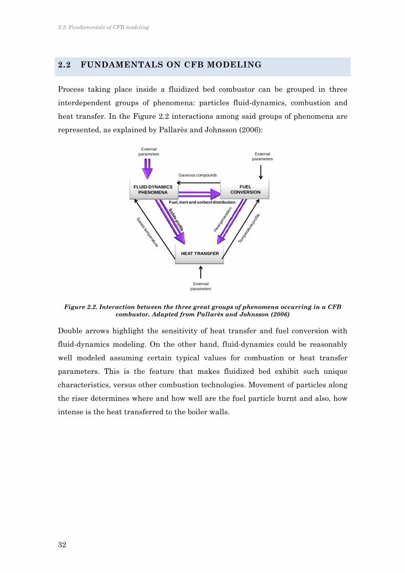
2.2. Fundamentals of CFB modeling
32
2.2 FUNDAMENTALS ON CFB MODELING
Process taking place inside a fluidized bed combustor can be grouped in three
interdependent groups of phenomena: particles fluid-dynamics, combustion and
heat transfer. In the Figure 2.2 interactions among said groups of phenomena are
represented, as explained by Pallarès and Johnsson (2006):
Figure 2.2. Interaction between the three great groups of phenomena occurring in a CFB combustor. Adapted from Pallarès and Johnsson (2006)
Double arrows highlight the sensitivity of heat transfer and fuel conversion with
fluid-dynamics modeling. On the other hand, fluid-dynamics could be reasonably
well modeled assuming certain typical values for combustion or heat transfer
parameters. This is the feature that makes fluidized bed exhibit such unique
characteristics, versus other combustion technologies. Movement of particles along
the riser determines where and how well are the fuel particle burnt and also, how
intense is the heat transferred to the boiler walls.
FLUID-DYNAMICS PHENOMENA
FUEL CONVERSION
HEAT TRANSFER
Fuel, inert and sorbentdistribution
Gaseous compounds
Externalparameters
Externalparameters
Externalparameters

Ref Type Scope Hydrodinamics
Fragm. Combustion
SOx Capture
NOx
HT Validation /Scale
Level Zones Phases Devolatilization Coal
combustion Shrinking Gen Rad
(Adánez and Diego, 1995)
CFB A II A B A C Y B C C D N
(Aibéo and Pinho, 2003) CFB A II B B ? A B N (Arena et al., 1995) BFB & CFB A I A B Y A C ? C D N (Krzywanski et al., 2010b)
OXY-CFB B II B C A D N B B B B N
(Seddighi et al., 2010) OXY-CFB A II B A A C N D C A B N (Chen and Saxena, 1977)
BFB? A I A A N F A N B C D C Y Literature
(Sotudeh-Gharebaagh et al., 1998)
CFB A I A A N A D N B B D D Y 800 kW
(Gungor, 2009) CFB A II B B A C ? B D Y 50 kW
(Gayan et al., 2004) CFB A II B Y D C Y D C C D Y 300 kW 100 kW
(Adanez et al., 2001) Turbulent A II A B A C Y B C C D Y 300 kWth
(Alagöz, 2006) BFB A I A B A C ? B C A C Y 300 kWth
16 MW
(Chen and Xiaolong, 2006)
CFB DYN B II Y C C ? B B A B Y
410 t/h Pyroflow
CFB (Steady state)
(de Souza-Santos, 2007) BFB I B ? Y 1.6 MW (Werner, 2001) CFB A II A B N A E Y 0.25m2
(Gungor and Eskin, 2008)
CFB A III B B Y A D Y D D B D? Y 50 kW
160 MW (literature)
(Wang et al., 1999) CFB C II A B Y A D N B B A A Y 12 MW (Huilin et al., 2000) CFB A II B B Y A D Y B C A A Y 30 MW (Romeo and Cortés, 1998)
PFB A II B B N A A N C C B B Y 80 MW
(Hannaes et al., 1995) CFB B III B B Y E C Y B B B B Y 120 MW (Lee and Kim, 1999) CFB A II B B Y A D Y B C A A Y 200 MWe (Werther et al., 2009) CFB B III A B Y C C Y D C D D Y 252 MWt (Vepsalainen et al., 2009)
CFB A IV E D B B Y
370 MWt
Table 2.1. Models of fluidized bed combustors
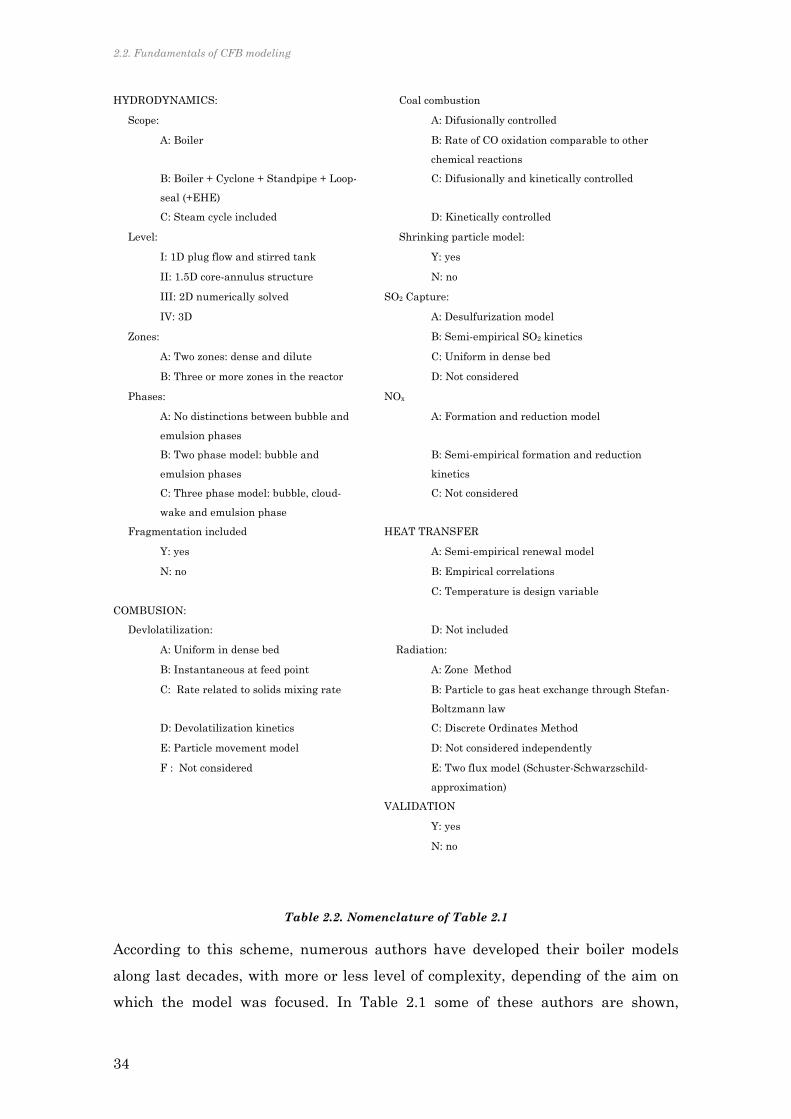
2.2. Fundamentals of CFB modeling
34
HYDRODYNAMICS: Coal combustion
Scope: A: Difusionally controlled
A: Boiler B: Rate of CO oxidation comparable to other
chemical reactions
B: Boiler + Cyclone + Standpipe + Loop-
seal (+EHE)
C: Difusionally and kinetically controlled
C: Steam cycle included D: Kinetically controlled
Level: Shrinking particle model:
I: 1D plug flow and stirred tank Y: yes
II: 1.5D core-annulus structure N: no
III: 2D numerically solved SO2 Capture:
IV: 3D A: Desulfurization model
Zones: B: Semi-empirical SO2 kinetics
A: Two zones: dense and dilute C: Uniform in dense bed
B: Three or more zones in the reactor D: Not considered
Phases: NOx
A: No distinctions between bubble and
emulsion phases
A: Formation and reduction model
B: Two phase model: bubble and
emulsion phases
B: Semi-empirical formation and reduction
kinetics
C: Three phase model: bubble, cloud-
wake and emulsion phase
C: Not considered
Fragmentation included HEAT TRANSFER
Y: yes A: Semi-empirical renewal model
N: no B: Empirical correlations
COMBUSION:
C: Temperature is design variable
Devlolatilization: D: Not included
A: Uniform in dense bed Radiation:
B: Instantaneous at feed point A: Zone Method
C: Rate related to solids mixing rate B: Particle to gas heat exchange through Stefan-
Boltzmann law
D: Devolatilization kinetics C: Discrete Ordinates Method
E: Particle movement model D: Not considered independently
F : Not considered E: Two flux model (Schuster-Schwarzschild-
approximation)
VALIDATION
Y: yes
N: no
Table 2.2. Nomenclature of Table 2.1
According to this scheme, numerous authors have developed their boiler models
along last decades, with more or less level of complexity, depending of the aim on
which the model was focused. In Table 2.1 some of these authors are shown,

Chapter 2. Large oxy-fuel circulating fluidized bed boiler modeling
35
attending at the strategies of modeling followed by each of the aforementioned
fields.
2.2.1 FLUID-DYNAMICS
A very extensively used and experimentally confirmed way of modeling fluidized
beds divides the combustor into several zones in which particles movement is
different and so they are the processes taking place in each region. In the bottom
part of a fluidized bed, a dense zone is clearly distinguished. Above this zone,
concentration of solids decays dramatically. Some researchers include in their
models an intermediate zone called splash zone. At the top of the riser, a fourth
region can be considered, the exit zone, very much dependant of exit geometry. In
Table 2.1 this division is shown in the corresponding column, distinguishing
between those authors that consider dense and dilute zones (Adánez and Diego,
1995; Arena et al., 1995; Sotudeh-Gharebaagh et al., 1998; Wang et al., 1999;
Adanez et al., 2001; Werner, 2001; Alagöz, 2006; Werther et al., 2009), and those
that also include spares and exit zones (Hannaes et al., 1995; Romeo and Cortés,
1998; Lee and Kim, 1999; Huilin et al., 2000; Aibéo and Pinho, 2003; Gayan et al.,
2004; Gungor and Eskin, 2008; Gungor, 2009; Krzywanski et al., 2010b; Seddighi
et al., 2010).
The bottom zone
This region occupies a small volume in the overall CFB combustor, above the
distributor, up to a height of around half a meter in large boilers. It is in this
region, where particle density is hundred times higher than in the rest of the boiler
and thus, most of combustion and chemical reactions occur here.
The way of modeling the bottom zone can be as simple as considering it a well
mixed stirred tank or assuming the two-phase model or even including the cloud-
wake phase and the mass transfer between the phases. The common point among
these treatments is assuming that the bottom zone behavior is similar to that
found in a bubbling bed regime. This was confirmed for example, with the
experiments made by Svensson et al. (1996), that found that increasing fluidization
velocities makes an increase in gas flow through the bubbles and the bubble
dynamics, showing fluctuation frequencies similar to those in bubbling beds,
around 1 Hz. In spite of these fluctuations generated by bubbles, dense bottom bed

2.2. Fundamentals of CFB modeling
36
has a quite uniform time-average void fraction. One of the main characteristics of
the bubbling bed regime, observed in the dense part of a CFB, is the linear time-
averaged vertical pressure drop profile above the distributor, as confirmed by the
authors. If an homogeneous mixing is assumed, i.e. the effect of the particle side
distribution (PSD) on jetsam/flotsam segregation can be neglected, void fraction
along the dense bottom zone is also constant. It can be expressed as:
emulsionbbb εδ1δε Eq. 2.4
According to the two-phase model, bottom zone consists of a dense or emulsion
phase, formed by bed particles and the interstitial flow between the particles; and a
bubble phase, made of uprising gas bubbles, considered to be free of solids (Kunii
and Levenspiel, 1991). First approaches assumed that all the gas in excess of umf
flowed through the bed as bubbles, while the emulsion stayed at minimum
fluidizing conditions. The expression for a single bubble rise velocity yields then:
21
bbr gd0.711u Eq. 2.5
However, there have been experimental evidences that the flow of bubbles is
overestimated by this assumption (Shen et al., 2004). This is because gas crosses a
certain section of the bed, not only by translation of bubble voids, but also by the
flow through the bubbles relative to them and the interstitial flow relative to the
particles in the dense phase. So, the overall gas balance would fulfill the following
expression:
vismftf uuuu Eq. 2.6
where the visible flow, uvis, would yield:
bbvis uδu
Eq. 2.7
Or it can be also expressed as the dimensionless visible bubble flow, Ψ:
mf
vis
uu
uψ
Eq. 2.8
Several empirical expressions have been proposed and used by researchers for
estimating the bubbling velocity. Some of them are summarized in Table 2.3.

Chapter 2. Large oxy-fuel circulating fluidized bed boiler modeling
37
Reference Correlation
Farrokhalaee (1979) in (Davidson et al., 1985)
D0.24xexpHu0.44uuu 0.230.32
mf0.62
b Eq. 2.9
Peters et al. (1982) in (Davidson et al., 1985)
mfb u-uYu
2mfmf uu5uu0.130.785Y Eq. 2.10
Werther (1983) in (Kunii and Levenspiel, 1991)
br1.35t
0.5bmfb ud1.13duu1.6u Eq. 2.11
Werther and Wein (1994) in (Pallarès and Johnsson, 2006)
0.181.45Arψ Eq. 2.12
Johnsson et al. (1991) in (Pallarès and Johnsson, 2006)
40CFB A4hfψ
ref5
b1
CFB ΔP102.6116.6d0.129u0.3121f
refΔP being the pressure drop between riser
height interval from 0.135 to 1.635 m above gas distributor
Eq. 2.13
Eq. 2.14
Table 2.3. Correlations for estimating bubble velocity
The transport zone
When bubbles reach the limit of the dense bed they explode in the surface.
Aggregates of particles are thrown into the splash zone. Due to the differences of
particles physical properties, drag forces per unit weight also differs from one type
of particle to another. A high drag force per unit weight makes the particles move
upwards, whereas particles with low drag per unit weight will tend to sink to the
bottom. During this instantaneous explosion of bubbles in the bottom bed surface,
competition between both mechanisms, mixing and segregation, occur
simultaneously. A strong back-mixing is caused in this region by the decay in the
solids concentration. The transport region comprises the height between the dense
bottom zone limit and the top of the riser. For covering both, the upper diluting and
the lower dense regions, the following expression was proposed by Li and Kwauk in
1980 (Horio, 1997):
isb
sp zzaexpεε
εε
Eq. 2.15
This way of modeling back-mixing and decay of solids concentration in the
freeboard has been extensively used by most of models in Table 2.1

2.2. Fundamentals of CFB modeling
38
The decay constant for these models, a, is inversely proportional to the gas velocity.
It represents fairly well the effect of the back-mixing of solids above the dense bed,
dominated by clustered solids thrown up into the freeboard.
For this reason, Johansson and Leckner (1995) proposed a two-solid-phase model,
consisting of a cluster and disperse phases. The first, describing a ballistic type of
solids back-mixing, similarly to Eq. 2.15 and the second, dominating the
contribution of the wall layer falling solids effect. The formed clusters in the dense
bottom zone are immersed in the disperse phase but there are few that reach the
top of the riser. So, particles are elutriated from the bottom rising upward along
the central region of the riser. In this region, the flow is turbulent due to high slip
velocities (the difference between the mean interstitial gas velocity and the mean
upward particle velocity) and particles are thrown towards the wall. A falling film
is then formed. This falling layer captures particles close to it and those particles
are entrained back to the core less frequently. This makes the concentration of
solids along the riser height adopting an exponential shape (Davidson, 2000). The
expression derived by Johansson and Leckner (1995) including the mentioned
back-mixing processes yields:
zHKexpρHzaexpρρρ exitexitxhdisp,bb Eq. 2.16
Where a corresponds, as in Eq. 2.15, to the back-mixing from homogeneous
clustering flow in the splash zone. K is the decay coefficient for the back-mixing in
the wall-layer flow (Johansson et al., 2007). Zijerveld et al. (1997) calculated the
decay constant using Eq. 2.15 and Eq. 2.16 in three boilers, the 12MWth CFB, a
1.2m x 0.8m and a 0.083 m ID CFB. They found that Eq. 2.15 fails to predict
satisfactorily the concentration in the larger risers, so they suggest to avoid that
expression for those commercial CFBs.
The exponential behavior of solids along the riser is then due to the lateral
transport of solids from the core to the down-flow wall layer of solids. According to
Horio (1997) there are two other ways of modeling the lateral solids transfer. One
approach explains the core-annulus flow by the radial velocity distribution and
radial density profile. The other explanation is based on time-average mass and
momentum balances.
The wall thickness, tδ, is the distance between the riser walls to the point where
net flux of solids is zero in the vertical direction. This magnitude has been

Chapter 2. Large oxy-fuel circulating fluidized bed boiler modeling
39
extensively studied and several correlations have been proposed, like the one by
Harris et al. (2002):
0.0663
0.05850.0247s
δ
H
zHRe0.4014ε10.5
D
t Eq. 2.17
In general, a clear dependence of wall thickness on riser height is observed. Some
authors include the effect of solids circulation adding the average solids
concentration term within their expressions, like the one proposed by Bi et al
(1996). Johnsson et al. (1995) collected data from different unit sizes and
conditions. For large-scale CFB boilers, this decrease in wall-layer thickness
upwards is also observed. This reduction levels out for (H-z)/Dequiv > 6 from where
a height-independent value for tδ was proposed. Therefore, the expression for the
wall-layer thickness was:
zH0.0108tδ for ductsat HzH
Eq. 2.18
and
equivδ 0.0648Dt for satb HzH Eq. 2.19
Gas composition seems to influence slightly on the explained theory of large one-
dimensional fluid-dynamics modeling. The models including oxy-fuel conditions on
their fluid-dynamic modeling do not include variations of the semi-empirical
approaches developed for air-firing. However, few studies have been published
lately, showing certain differences on the bubbling regime for high CO2
concentration in the fluidizing gas, specially related to changes in viscosity and
density (Guedea et al., 2011).
2.2.2 COMBUSTION AND POLLUTANT FORMATION
When a fuel particle enters the bed, the following processes take place:
‐ Heating and drying
‐ Devolatilization and volatile combustion
‐ Swelling and primary fragmentation
‐ Char combustion

2.2. Fundamentals of CFB modeling
40
The typical bulk temperature in fluidized bed boilers is over 800ºC. Then, at 100ºC
heating and drying of the particles happens quickly and can be considered to occur
almost completely in the dense part. Volatile content is considered a property of
coal. There are methodologies to estimate the portion of carbon on volatiles but, in
fact, to quantify coal volatile content, temperature, heating rate and particle
diameter should be considered (Thunman et al., 2001). When a detailed model of
the particle combustion is needed, fragmentation of the fuel particle must be
regarded. Fragmentation takes place when steam or volatiles inside the particles
are released, but the pore structure of the fuel particle does not let them escape.
Thus, higher pressure is generated inside the particle and it can be then broken.
One of the consequences of fuel particle fragmentation is the unburnt carbon
entrainment (Daki et al., 1989).
In the range of 400-900ºC the temperature has a positive influence on the quantity
of volatiles. If heating rates are below 600ºC/s, less volatile matter is released. In
the case of lignites, it does not depend on pressure but for bituminous coals
decreases with increase of pressure (Oka, 2003).
For understanding the devolatilization and volatile combustion of a single coal
particle inside a fluidized bed, the study by Prins et al. (1989) gave a
comprehensive data analysis. Huilin et al. (2000) suggested the expression
developed by Peter and Poynton in 1992 for estimating the devolatilization time:
pg
VOL dT
104810t
Eq. 2.20
Devolatilization time, tVOL, is very short and depends mainly on temperature, Tg,
and particle diameter, dp. As seen in Table 2.1, most of models assumed that
devolatilization occurred in the dense part of the fluidized bed, uniformly
distributed along the bottom bed height. This is the assumption considered in this
work.
Regarding char combustion modeling, it is often carried out including a kinetic
model, like the one used by Huilin et al. (2000), Gungor and Eskin (2008) or
Sotudeh-Gharebaagh et al. (1998). Some authors also included the diffusion mass
transfer in their models. The shrinking unburned core model has been extensively
used in these kind of detailed combustion model. Thus the shrinking rate of the
particle radius could be expressed like suggested by Adánez and de Diego (1995):

Chapter 2. Large oxy-fuel circulating fluidized bed boiler modeling
41
g
p
cccchar
Oi
ShD
d
K
1xρ
12C
dt
dr2
Eq. 2.21
Where CO2 is the concentration of O2 around the particle; Kc is the kinetic constant
of burning char particles; Sherwood number is semi-empirically estimated, using
two different expressions for the dense part and for the dilute zone; and Dg is the
diffusivity of oxygen in nitrogen.
Fuel conversion in oxy-fuel fluidized beds was explored by the team from
Czestochowa Technical University (Czakiert et al., 2006). They made experiments
for different O2/N2 mixtures and compared it with O2/CO2 mixtures. Carbon
conversion ratio increased with increasing oxygen concentration in the gas
mixture, regardless the reactor’s temperature level. This was explained because
combustion rate increased by an increase in oxygen partial pressure. Increasing
temperature had no effect on carbon conversion ratio. The carbon conversion in the
O2/N2 mixtures was always higher than for O2/ CO2 mixtures, at the same oxygen
concentration and combustor temperature. Tests reported by Nsakala et al. (2004)
in the ALSTOM Multi-fuel CFB also observed, as expected, higher CO emissions,
likely due to high CO2 content of the flue gas, which hinders oxidation of CO.
Still, the influence of atmosphere on char combustion during oxy-fuel fluidized beds
is not evident, as explained by Guedea et al. (2013). Char reactivity changes with
varying the diluting gas in the atmosphere, but it is related with higher volatile
matter content and porous residual char. Higher reactivity was found under O2/N2
atmosphere, due to higher diffusivity coefficients. On the other hand, in some
cases, higher O2 concentration implied higher velocity of reaction, concluding that
different fuels are not affected in the same way by oxy-fuel conditions.
SO2 formation
One of the main advantages of burning coal in fluidized bed is the capacity of in-
furnace SO2 capture, when adding a proper solid sorbent. This sorbent is usually
limestone or dolomite mineral stones which do not influence the combustion
process. Under certain conditions, they calcined, i.e. calcite crystals (CaCO3)
disintegrate into small lime crystals (CaO) due to CO2 diffusion, according to the
reaction:

2.2. Fundamentals of CFB modeling
42
23 COCaOCaCO R. 2.1
The resulting porous structure depends on limestone and calcination conditions,
i.e. temperature and CO2 partial pressure, and dominates the subsequent sulfation
phenomena:
422 CaSOO SO CaO 2
1 R. 2.2
Under conventional atmospheric air-firing conditions, where CO2 partial pressure
is around 0.12-0.15 bar, calcination takes place above 790ºC. Then, SO2 and O2
penetrate through the pores and react with CaO yielding CaSO4. Formed CaSO4
will not decompose until approximately 1580ºC, so it is thermodynamically stable
at a range of conventional bed temperatures of 800-1000ºC. This is one of the
reasons of keeping fluidized bed temperature within the mentioned range.
Optimum desulfurization temperature is commonly accepted to be located near
850ºC. Nevertheless, this optimum temperature depends on sorbent properties and
combustion conditions. For example, Mattison and Lyngfelt (1999) found that
under alternating conditions, CaSO4 reacts with CO or H2, releasing SO2 and
breaking CaSO4 layer. Therefore SO2 capture efficiency is increased and optimum
temperature is also lower than under oxidizing conditions.
By analyzing the equilibrium between CaO and CaCO3, high CO2 partial pressure
does not let limestone to be calcined at conventional air-firing temperature and
sulfation takes place in one step, also called direct sulfation:
24223 COCaSOO SO CaCO 2
1 R. 2.3
Direct sulfation was previously addressed for pressurized fluidized beds (Snow et
al., 1988), but it can also happen under atmospheric oxy-fuel combustion. The effect
of CO2 partial pressure on limestone conversion is commonly expressed with
equilibrium pressure term, Peq, at bed temperature, that coincides with the
equilibrium constant of reaction, estimated from thermochemical data (García-
Labiano et al., 2002):
T
20474exp104.137P 12
eq Eq. 2.22
Calcination rate becomes lower when PCO2 is increased. Figure 2.3 shows this
tendency, represented by the expression (Stanmore and Gilot, 2005):

Chapter 2. Large oxy-fuel circulating fluidized bed boiler modeling
43
CO2eqDc PPkR Eq. 2.23
T
40261.22expkD Eq. 2.24
Figure 2.3. Dependence of calcination rate on partial pressure and temperature
When PCO2 is above Peq, CO2 cannot migrate out the sorbent particle, preventing
calcination (García-Labiano et al., 2002). Nevertheless, although desulfurization
rate is lower than in indirect process, CaSO4 layer formed around the particle core
has more and larger porous, allowing a higher Ca conversion (Hu et al., 2006). This
improvement depends strongly on particle size and residence time (Liu et al.,
2000). Unlike in indirect sulfation, there is no agreement on an optimum
temperature for direct sulfation (Qiu and Lindqvist, 2010).
Since CO2 partial pressure under oxy-firing atmospheres significantly differs from
air-firing, desulfurization reaction mechanisms also change. For typical bed
temperatures (800-900 ºC) and near to atmospheric pressure, direct sulfation takes
place instead of the indirect sulfation, similarly as in PFB. De Diego and co-
workers (de Diego et al., 2011; García-Labiano et al., 2011) analyzed the influence
of temperature, particle size and CO2 concentration during sulfation under oxy-
firing conditions on desulfurization process in a thermogravimetric balance. They
found lower particle conversion in direct sulfation which improved at higher
temperature. The contrary happened for indirect sulfation. First results published
about desulfurization under oxy-firing conditions in a CFB do not reveal a clear
tendency of desulfurization efficiency using the same Ca:S ratio. Jia and co-
workers (2010), reported lower efficiencies using two kinds of limestones and coals
whereas Duan and co-workers (2011b) obtained higher values under oxy-firing for
an anthracite and a bituminous coal with a similar CaO content in limestone
(around 53%of CaO).
0 0,4 0,8 1,2 1,6 2
0,02
0,04
0,06
0,08
CO2 Partial pressure, PCO2 (atm)
Ca
lcin
atio
n ra
te o
f lim
esto
ne, R
c (m
ol/m
2 s)
850ºC
950ºC950ºC

2.2. Fundamentals of CFB modeling
44
However, several studies confirm that indirect sulfation also occurs under oxy-fuel
bed combustion if the temperature is high enough, and consequently
desulfurization rate sharply increases, as shown in Figure 2.3. Higher bed
temperature is required during oxy-fuel combustion for reaching similar SO2
capture efficiency.
In the current model, SO2 capture will be implemented because of its influence on
CO2 emissions and, mainly, in the energy balance. Calcination is an endothermic
process, whereas sulfation is exothermic. Thus, SO2 capture by the indirect way
would consume heat of combustion if CaCO3 excess is used.
NOx formation
During coal combustion, NOx is originated from the nitrogen present in air or from
the N-fuel. Air-nitrogen generates NOx at high temperature (thermal process), that
are not usually reached in fluidized beds. It can be formed also by the prompt
process, but this is not usual process in fluidized bed, since hydrocarbon free
radicals and high temperature would be necessary. So 95% of NOx in a fluidized
bed is formed from the fuel nitrogen. During devolatilization, when coal particle is
heating-up, nitrogen decomposes to yield gaseous HCN as the main nitrogen-
containing specie. This hydrogen cyanide then forms the basis for most reactions
leading to NOx in the gas phase (Hayhurst and Lawrence, 1996).
Destruction of formed NO is usual as well. It can react with other species such as
NH2 yielding N2. NO reduction is also possible with CH:
OHCNNO CH R. 2.4
This is the reaction that allows reburning, as a method for reducing NOx emissions,
feeding methane in the freeboard. Reburning can occur in fact during the
incomplete combustion of volatiles. However, if O2 is available, CH radicals
oxidized quickly yielding CO and CO2, before reacting with NO.
When fuel is present, NO can also be reduced by other species in atmosphere with
NH2:
OHNNH NO 222 R. 2.5
OHNNH NO 2 R. 2.6
Char particles also help to heterogeneous reduction of NO to N:

Chapter 2. Large oxy-fuel circulating fluidized bed boiler modeling
45
CONchar NO 2 R. 2.7
22
char
CON2
1CO NO
R. 2.8
Nitrous oxides, N2O, are formed similarly than NOx. It is formed from N-fuel and it
requires the same precursors: HCN and NH3. So, reactions yielding these
intermediate compounds are common for all nitrogen oxides:
COONNO NCO 2 R. 2.9
HONNO NH 2 R. 2.10
Bed temperature is an important parameter. According to de Diego et al. (1996)
bed temperature makes NOx emissions decrease but N2O increase. This influence is
even greater for higher air excess. Also, when incrementing air excess, NOx and
N2O increase. This is explained because higher O2 concentration increases volatile
and chars combustion and also, at the same time, concentration of char and CO is
lower, so heterogeneous reduction of NO is decrease in the char surface.
N2O is also increase by higher volatile (NH3 and HCN) conversion via homogeneous
reactions as:
HNCOO HCN R. 2.11
COONNO NCO 2 R. 2.12
NOx and N2O is reduced by increasing secondary air injection. This is an
extensively used method for control of pollutants. This is because combustion
occurs in oxygen-limited conditions, favoring volatile conversion from N to N2,
instead to NOx. Moreover, char is accumulated and higher CO concentration allows
decomposition of NO via CO (R. 2.8) in the char surface. Finally, residence time of
gas in the lower part increases. Thus, NOx decreases because NOx decomposition is
faster than NOx formation along the riser.
Mechanisms of formation and destruction for NO and N2O during fluidized bed
combustion have been thoroughly studied in the literature. A clarifying way of
understanding main conversion paths of fuel nitrogen during fluidized bed
combustion was explained by Leckner (1997) and it is schematically present in
Figure 2.4

2.2. Fundamentals of CFB modeling
46
Figure 2.4. Main conversion paths of fuel nitrogen. Adapted from Leckner (1997)
In oxy-fuel combustion there have been numerous investigations of NOx formation
specially in pulverized coal combustion. Experiments from the Czestochowa CFB
pilot plant (Czakiert et al., 2006) show a significant limitation of fuel-nitrogen
conversion to NOx during oxy-fuel combustion.
In the 50kW CFB in Southeast University in China the effect of operation
parameters of oxy-fuel combustion on NO emissions were analyzed by Duan et al.
(2011a). NO formation decreased in 21%/79% O2/CO2 atmosphere. They explained
it as due to the less O and OH radicals formed under lower bed temperature. In
addition, low temperature and high CO2 concentration bring possibility of higher
CO concentration in O2/CO2 atmosphere. As the O2 concentration at inlet is
increased gas velocity diminishes and this means longer residence time of fuel
particles in the combustor, which would promote fuel-N conversion into NOx
precursors. Increasing bed temperature or oxygen stoichiometric ratio brings
higher NO emission in O2/CO2 atmosphere, which is consistent with the results in
air-fired CFB combustion. Stream staging is more efficient for controlling NO
emission in oxy-CFB combustion than that in air combustion.
Another important issue in oxy-fuel is the positive effect of RFG on the decrease of
NO emissions. Okazaki and Ando (1997) examined the effects of CO2 concentration,
together with the less recycled-NO in the flame, and the interaction of fuel-N and
Nfuel
Nchar Nvol
NH3 HCN
NH2
N2
N2
N2
NO
N2ONO
N2ONO
N2O
N2N2
NO Nchar NH3 HCN N2O

Chapter 2. Large oxy-fuel circulating fluidized bed boiler modeling
47
recycled NOx on the decrease of the final NOx exhausted from the coal combustion
system with the recycled CO2. They concluded that the conversion ratio from the
fuel-N to exhausted NOx is reduced to less than one-fourth of that with air
combustion, and the effect of a reduction of recycled-NO in the furnace was
dominant and amount to 50%-80%.
In the current model, NOx formation and destruction reactions are not included,
since their energy interactions can be neglected, compared with combustion and
sulfation reactions.
2.2.3 HEAT TRANSFER
For decades, there have been numerous investigations on heat transfer in fluidized
bed, specially carried out in laboratory scale facilities. Although not completely
independent, there is a generalized treatment of heat transfer from bed to surfaces
as the contribution of three mechanisms: the transient conduction of particles
when contacting the surface, also called particles convection; the gas convection,
and the radiation heat transfer. In fast beds such as circulating fluidized bed, heat
transfer is strongly dependent on particles fluid-dynamics. Parameters like rate of
solids circulation, superficial velocity through the column, and particle size, will
define the dominant heat transfer mechanism. Particles travel upwards along the
core in the form of strands. When strands approach the wall layer, they change
direction. Therefore, energy is transferred from particle strands or agglomerates at
bed temperature that “enters” into the wall and exchange heat with the surface
during certain residence time. This is called renewal packet theory and it is further
explained in the next chapter.
Radiation heat transfer turns out the dominant heat transfer mechanism for the
low density boiler zones. Normally, gas-particle suspension can be considered
isothermal. Thus, the expression for the radiative heat transfer coefficient related
to a plane grey heat transfer surface follows the expression:
wb2
w2
bbwr TTTTσεh Eq. 2.25
Where

2.2. Fundamentals of CFB modeling
48
1ε
1
ε
1ε
wef
bw
1
Eq. 2.26
As stated by Baskakov and Leckner (1997) there is not a unique methodology for
accurately estimate the value of emissivity of an isothermal suspension. All those
methodologies coincide in indicating that particle emissivity is the main factor for
the suspension emissivity, so as particle porosity. For estimating values of the
radiative heat transfer, these authors separated the effect of gas phase convection
heat transfer from the measures values, calculating the gas contribution by the
expression:
0.430.8gc Pr0.003ReNu Eq. 2.27
The heat transfer coefficient in the membrane wall of the 12MWth CFB at
Chalmers was 104 W/m2K. Convection and radiation heat transfer coefficients were
estimated around 20 and 78 W/m2K respectively, confirming good fitting of
aforementioned assumptions.
Basu and Nag (1996) collected heat transfer data from several commercial CFB
units. Average heat transfer coefficients ranged from 80-220 W/m2K and shows
great dependency on suspension density. He correlated data against suspension
density and obtained the following expression:
nsaρh Eq. 2.28
with 40 and 0.5, for 5 25 /m and 750 850ºC. Similar
expressions were proposed by Divillo and Boyd (1994), where 23.2 and
0.55, although this was proven by Xie et al. (2003) to overestimate data for
densities greater than 200 kg/m3.
Basu and Nag (1996) explained the dependence of heat transfer in large units with
temperature. There is an obvious increase of heat transfer coefficient with
increasing temperature, due to higher gas thermal conductivity and higher
radiation. At a relatively high suspension density of 20 kg/m3 the increase in heat
transfer coefficient with temperature was linear. This may not be the case at a
more dilute bed where the radiation becomes dominant. Regarding fluidization
velocity there were not much influence on heat transfer in large units. It was
reported that change in secondary air rate did not affect the heat transfer

Chapter 2. Large oxy-fuel circulating fluidized bed boiler modeling
49
coefficient in the upper part of the furnace, but an increase in the primary air
velocity did increase it (Andersson and Leckner, 1992). This happened because the
increased primary air transported more solids to the upper section increasing the
suspension density in that region of the bed. Particle size had a strong effect in
laboratory units, but influenced much less heat transfer in large units. This is not
the case for bubbling fluidized beds where the particle size is the most important
factor influencing heat transfer irrespective of the plant size.
Breitholtz et al. (2001) reviewed heat transfer coefficients from laboratory and
industrial scale fluidized bed boilers and proposed an exponential simplified
expression for particle convection heat transfer that fit data of all the cases
studied. Considering the different mechanisms to transfer heat as independent
contributions, the overall bed-to-wall heat transfer could be expressed as:
maxr,rb
0rconv hηραhhh Eq. 2.29
Where hconv comprises particle and gas convection mechanisms and hrad is radiation
heat transfer coefficient. Parameters for the equation yields α0 = 25 and b = 0.58.
ηr refers to the radiation efficiency term, that gives an idea about the shadow effect
of the boundary layer. In the extremes cases, this term would becomes 1 for a very
thin optical wall layer, and 0.65 when optical layer is thick. ηr takes the form:
1.6
2.6
ρ arctan 0.140.86
rη s Eq. 2.30
This expression shows an asymptotical shape on the value 0.65, i.e., for dense wall
layer only 65% of the energy emitted by radiation will be seen by the wall.
Cheng and co-workers (2007) reviewed numerous measured heat transfer
coefficients in large fluidized beds. They measured heat transfer in a 12 MWe, 50
MWe and 135 MWe CFB boilers and observed again the high dependence of these
values with the solids concentration in the riser, and in different zones of the
boiler, such as the cyclone, and the economizer. They confirmed that it is mainly
influenced by solid suspension density and furnace temperature. They stated
following a correlation in the form of:
βs
αs TKρh Eq. 2.31
Being K, α and β regression coefficients, which are not specified in the paper. They
proposed this expression because in the review of large CFB most of expressions for
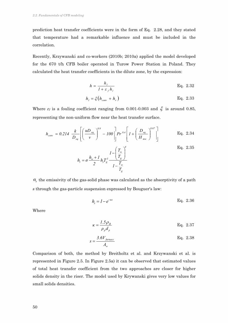
2.2. Fundamentals of CFB modeling
50
prediction heat transfer coefficients were in the form of Eq. 2.28, and they stated
that temperature had a remarkable influence and must be included in the
correlation.
Recently, Krzywanski and co-workers (2010b; 2010a) applied the model developed
for the 670 t/h CFB boiler operated in Turow Power Station in Poland. They
calculated the heat transfer coefficients in the dilute zone, by the expression:
1f
1
hε1
hh
Eq. 2.32
rconv1 hhh Eq. 2.33
Where εf is a fouling coefficient ranging from 0.001-0.003 and is around 0.85,
representing the non-uniform flow near the heat transfer surface.
0.67
mw
eq0.4
0.8
eq
eqconv H
D1Pr100
ν
uD
D
k0.214h Eq. 2.34
g
w
4
g
w
3gs
wr
T
T1
T
T1
Th2
1hσh
Eq. 2.35
sα the emissivity of the gas-solid phase was calculated as the absorptivity of a path
s through the gas-particle suspension expressed by Bouguer's law:
κss e1h Eq. 2.36
Where
pp
B
dρ
1.5κ
Eq. 2.37
w
furnace
A
3.6Vs
Eq. 2.38
Comparison of both, the method by Breitholtz et al. and Krzywanski et al. is
represented in Figure 2.5. In Figure 2.5a) it can be observed that estimated values
of total heat transfer coefficient from the two approaches are closer for higher
solids density in the riser. The model used by Krywanski gives very low values for
small solids densities.

Chapter 2. Large oxy-fuel circulating fluidized bed boiler modeling
51
Looking at the estimated values for radiative heat transfer, Figure 2.5b), in the
model of Krzywanski et al. they tend to zero for very low solids concentration, due
to the form of Eq. 2.13. The influence of particle densities shows opposite behavior
in the approach by Breitholtz et al. Denser riser leads to denser wall layer and the
shadow effect to the heat transfer surfaces increases, and thus, heat transfer by
radiation decreases. This is not the case of the expression used by Krzywanski et
al. since the term for suspension absorptivity makes denser medium leading more
intense radiation. The influence of the radiation path thickness is shown to
influence remarkably on the estimation of the radiation. This term is not
considered by Breitholtz et al. but the empirical term of radiation efficiency allows
taking density of wall layer into account.
Figure 2.5. Dependence of the a) total and b) radiative heat transfer coefficient with the bed density according to Beritholtz and Leckner (1997) and Krzywansky et al. (2010b) for
different radiating layer thickness, s
0 2 4 6 8 100
45
90
135
180
225
Average solids concentration (kg/m3)
Tot
al h
eat t
rans
fer
coef
ficie
nt (
W/m
2K
)
Krzywanski s=0.05m
Krzywanski s=0.1m Krzywanski s=0.1m
Krzywanski s=0.2m Krzywanski s=0.2m
Krzywanski s=0.3 m Krzywanski s=0.3 m
Breitholtz Breitholtz
0 2 4 6 8 1040
60
80
100
120
140
160
180
200
Average solids concentration (kg/m3)
Rad
iatio
n he
at tr
ansf
er c
oeff
icie
nt (
W/m
2K
)
Krzywanski s=0.05m
Krzywanski s=0.1m Krzywanski s=0.1m
Krzywanski s=0.2m Krzywanski s=0.2m
Krzywanski s=0.3 m Krzywanski s=0.3 m
Breitholtz Breitholtz
a)
b)

2.3. The oxy-fuel CFB model
52
In none of the aforementioned models, radiative gas properties influence
appreciably the radiative heat transfer coefficient. This is not the case for heat
transfer in pulverized coal boilers, where radiation from the flame through the gas
is the dominant heat transfer mechanism.
It is generally assumed that heat transfer under oxy-fuel combustion conditions
behaves similarly to air-firing conditions, i.e. main parameters influencing heat
transfer such as bed temperature, particles concentration, particles diameter or gas
velocity affects heat transfer the same way as it does under oxy-fuel conditions.
However, there are no experimental published data about this issue and models
available in the literature takes the same models used for air-combustion.
2.3 THE OXY-FUEL CFB MODEL
The overall model for the OF in CFB has been sub-divided into three non-
independent modules that interact with each other as shown in Figure 2.2: i) solids
fluid-dynamics, ii) combustion and iii) energy balance. The sequence of sub-models
arranged for CFB modelling is represented in Figure 2.6. Main initial
considerations are following explained, for understanding the significant
operational factors that would determine the overall CFB behaviour.
‐ Fuel input and fuel characteristics: Thermal power input is determined by
fuel rate and by its composition and heating value. These parameters allow
calculation of stoichiometric O2 needed plus certain excess for assuring
proper combustion. In the case of air combustion, an air-excess around 20%
is generally accepted to reach around 3-6 % O2 in flue gases. Similar oxygen
contents in flue gas have been considered in the OF simulations. In any
case, the fuel thermal input imposes the amount of oxidant flow.
‐ Inert matter properties: Main fluidization parameters such as fluidization
velocity or terminal velocity are determined by the particle density of the
bed material and particles size distribution, among other factors. A solids
inventory consisting of particles with a diamter of 200 μm and a density of
2500 kg/m3 (Geldart B type) has been assumed.
‐ Boiler geometry. The amount of gas entering the boiler and the boiler cross
sectional area will settle the fluidization velocity and thus, how solids will

Chapter 2. Large oxy-fuel circulating fluidized bed boiler modeling
53
be distributed along the riser. Secondary gas inlet is located at 5 m height
from the distributor.
‐ Pressure drop along the combustor: This parameter is easily measured with
conventional pressure taps and bottom bed height can be estimated. Values
around 9000-12000 Pa have been considered as average range on
conventional air firing boilers. Thus, the pressure drop limits the height of
the lower dense region (Yang et al., 2005; Redemann et al., 2009; Lu et al.,
2010)
The first sub-module in the programme aims to estimate the solids concentration
profile for certain fuel input, boiler geometry and pressure drop across the boiler. It
calculates fluid-dynamics in the dense and in the transport zones, such as void
fraction, gas velocity and wall layer thickness at every height. For estimating gas
properties, temperature profile must be an input that will be calculated in the
energy balance sub-model.
Figure 2.6. CFB model flow-chart

2.3. The oxy-fuel CFB model
54
The combustion module calculates the main formed species based on disperse and
cluster phases present at each cell. Temperature must be also an input for
estimating if calcination of limestone takes place before sulfation, according to Eq.
2.22.
Finally, the energy balance sub-module will carry out the energy balance cell by
cell, according to the combustion, heating of gases, heat carried by the solids and
cooling at each height.
In Figure 2.7 it has been graphically represented the processes taking place in each
part of the control volume considered in this model. Black arrows represent the
flux of solids, modeled by the fluid-dynamic module, where primary and secondary
gas are the inlets, so as the boiler geometry and pressure drop. Red circle arrows
represent the heat of reactions. As can be seen, combustion in the loop-seal was not
considered. During air firing combustion, unburnt fine particles are likely to be
burnt by the O2 present in the fluidizing gas. However, O2 in the fluidizing gas of
the EHE will be avoided, for economical reasons.
Figure 2.7. CFB boiler mass and energy balance scheme
Primarygas
Fuel
Secondarygas
Recycledparticles
Flue gas
Waterwalls
ExternalHeat
Exchange
Convectivepass
Particles
Gas
Combustion
Energy

Chapter 2. Large oxy-fuel circulating fluidized bed boiler modeling
55
2.3.1 FLUID-DYNAMICS SIMULATION
The fluid-dynamics simulation sequence is represented in Figure 2.8. Input
parameters are:
1. Fuel input. During AF, this is given by the fuel input considered and so, by
the stoichiometric O2 required for combustion, plus a certain excess, for
assuring adequate efficiency of combustion. For OF case, a higher O2
concentration allows to introduce higher fuel inputs for a certain fluidizing
velocity. Thus, the fuel feeding rate sets the volumetric flow of gases
entering into the boiler.
2. The secondary gas ratio. Although it is evident that in real boilers there are
several secondary air entrances, for the scope of this model, one secondary
gas inlet is considered. By calculating the volumetric inlet gas required,
together with the secondary gas ratio, the primary gas is calculated and
then, the fluidizing velocity at the entrance of the distributor plate.
3. The pressure drop along the riser. In many simulations found in the
literature, the entrained solids flow, Gs, and the dense bed height are
estimated using semi-empirical expressions. However, in the current model,
it has been considered that in a real boiler, certain pressure drop along the
boiler can always be measured and reasonable values for these parameters
are generally known. Thus, riser pressure drop will be an input parameter
for the model
4. The model is developed using monosize inner matter particles and thus, no
attrition is included.
Main assumptions used in the fluid-dynamical module are:
i. The bed is divided into two zones, the bottom dense bed and the transport
zone
ii. Core-annulus structure is assumed in the transport zone
iii. Two-phase theory is used for calculating properties in the dense phase,
according to Eq. 2.13.
iv. Dilute and cluster phases are considered for calculating the distribution of
solids along the riser, Eq. 2.16
v. PSD has not been included, and particles are considered monosize, with a
average particle diameter of 200 microns
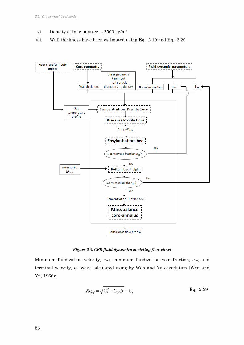
2.3. The oxy-fuel CFB model
56
vi. Density of inert matter is 2500 kg/m3
vii. Wall thickness have been estimated using Eq. 2.19 and Eq. 2.20
Figure 2.8. CFB fluid-dynamics modeling flow-chart
Minimum fluidization velocity, umf, minimum fluidization void fraction, εmf, and
terminal velocity, ut. were calculated using by Wen and Yu correlation (Wen and
Yu, 1966):
1221mf CArCCRe Eq. 2.39
Chapter 2. Large oxy-fuel circulating fluidized bed boiler modeling
57
g
pmfgmf μ
duρRe
Eq. 2.40
where C1=27.2 and C2=0.0408. And for minimum fluidization void fraction, Ergun
correlation was solved (Ergun and Orning, 1949):
ArReφε
)ε150(1Re
φε
1.75mf2
s2mf
mf2mf
s3mf
Eq. 2.41
Bottom bed voidage, so as bubble properties were estimated with Eq. 2.4 –2.9 and
Eq. 2.13 – 2.16. Wall layer thickness followed Eq. 2.18 –2.20.
The solids concentration along the riser considered the contribution of the cluster
and dilute phase, Eq. 2.16, being the decay constants:
u(z)
u4a(h) t Eq. 2.42
tuu(z)
0.23K(h)
Eq. 2.43
The decay constants depend on the gas velocity in riser. This velocity could vary if
boiler geometry does, so as with secondary gas injection. And also, the temperature
profile and the gas composition will vary gas velocity with the height of the riser.
Knowing the solids profile along the boiler, pressure drop profile is calculated:
(h)gz(h)ΔP coreriser Eq. 2.44
From this calculation, ΔPref is re-calculated and used for the iterations of the
bottom bed voidage. For estimating the height of the dense zone, pressure drop
measurements must be compared with the calculated pressure drop and so, by
interpolation, a new hbb is calculated and introduced in the sequence again.
Once the core solids concentration profile is calculated, the solids up-flow in the
core region, mcore, becomes:
(z)(z)u(z)A(z)m slipetransv_corcorecore Eq. 2.45
Being the slip velocity:
(z)uu(z)(z)u tslip Eq. 2.46

2.3. The oxy-fuel CFB model
58
Up-raising solids decrease with boiler height, because some are transferred to the
wall and falls down contributing to create the downward flow of solids in the so-
called annulus. Thus:
dz)(zm(z)m(z)m corecorelat Eq. 2.47
(z)mdz)(zm(z)m latwallwall Eq. 2.48
The exponential decrease of solids with height, explained for solids concentration
profile, was, in fact, experimentally verified for the solids mass flow. Application of
Eq. 2.47 and Eq. 2.48 implied then these intrinsic assumptions:
- no dependency of velocity with height
- no dependency of core cross sectional area with height
With the aim of compensating mistakes dragged by these assumptions an
additional term is included in the concentration profile expression:
core
core
slip
slipclusterdispcore A
A
u
u(z)(z)(z) BBBB Eq. 2.49
This fluidynamics modeling calculates the solids density distribution along the
whole boiler height and thus, also, the elutriated solids and the density and
thickness of the wall layer of particles. This sequence must be up-dated with the
values obtained from the combustion modeling, to account for the gas composition,
and from the heat transfer modeling, to account for the temperature at every
height.
2.3.2 COMBUSTION SIMULATION
Combustion modeling sequence is represented in Figure 2.9. Results from the fluid-
dynamics module are the main inputs of this module. Coal proximate and ultimate
analysis are needed, on the one hand for calculating the volatile composition and
also, for setting-up the carbon combustion at each height. As seen in Figure 2.9 the
temperature profile from the energy balance module is also an input. This input
will be applied for determining the mechanism of SO2 capture according to Eq.
2.22.

Chapter 2. Large oxy-fuel circulating fluidized bed boiler modeling
59
Figure 2.9. CFB combustion modeling flow-chart
Table 2.4. Coal composition used in the simulations
Spanish lignite
Central Europe
Antrhacite
ANALYSIS DATE 22/02/2010 03/11/2010
HHV (Kcal/kg) 3420 7124
INMEDIATE
Moisture 19,98% 2,04%
Volatile 23,81% 17,10%
Fixed C 28,15% 68,82%
Ash 28,05% 12,04%
ELEMENTAL
C 37,52% 75,86%
S 6,16% 0,38%
H 3,77% 3,44%
N 0,26% 1,95%
O 24,24% 6,33%

2.3. The oxy-fuel CFB model
60
Volatile content in coal was considered as a coal property. Volatile composition was
not known and needed to be estimated. Firstly, the methodology used by Thurman
et al. (Thunman et al., 2001) was applied on two different coals considered for
simulations: Spanish lignite and anthracite from Central Europe. Both coals
compositions are shown in Table 2.4.
Calculations of volatile composition are based on the mass balance of O, H and
volatile C, yielding CO2, CO, H2, H2O and CH4. This composition is also assumed by
Hannes et al. (1995). Volatile heating value can be estimated from the balance:
LHVvolatile = LHVfuel – (LHVdrying + LHVdevolatilization + LHVchar ) Eq. 2.50
Mass and energy balance of volatile compounds gives a degree of freedom that
could be solved by iteration. Energy for water vaporization and devolatilization is
small compared with the rest of terms, so approximation values have been
considered:
LHVdrying = 2253 kJ/kg
LHVdevolatilization = 300 kJ/kg
Hence, equations system yields:
x C = αCO2 + β CO + γCH4
y H = δ/2 H2O + γ/4 CH4 + ε/2 H2
z O = α/2 CO2 + βCO + δH2O
β ΔHCO + γ ΔH CH4 + ε ΔH H2 = LHVvolatile
This system has five unknown variables and four equations. The variables α , β , γ ,
δ and ε, are the molar rate of each component. The way of solving would be giving
values to one of the unknowns. The system would look like:
volatileHCHCO
LHVz
yx
HHH
2
0
00211
21
4100
0111
24
Eq. 2.51
Applying this methodology to the aforementioned coals found no convergence.
Then, they were also included other components to the calculations, such as C6H6,

Chapter 2. Large oxy-fuel circulating fluidized bed boiler modeling
61
C2H6, C2H4 and C2H2. In none of the runs convergence on the volatile composition
was reached. In the Figure 2.10, some of the simulations are shown: In Figure
2.10a), the basics components and in Figure 2.10b), C6H6 is added.
Figure 2.10. Simulations results of non-convergence of applying volatile composition methodology, considering. a) CO2, CO, H2, H2O and CH4; b) CO2, CO, H2, H2O, CH4 and C6H6
There is no point in which all parameters are above zero and below 100%, so no
feasible solution is possible considering these compounds. The same occurred when
adding other compounds to the iterations of Eq. 2.51. Possible causes of this lack of
convergence could be that this methodology was developed for biomass fuel, with a
higher volatile content than coal. An alternate possibility of estimating volatile
0 20 40 60 80 100-10
0
10
20
30
40
50
60
70
CH4 (%)
CO
, C
O2,
H2,
H2O
(%
)
COCO
CO2CO2
H2H2
H2OH2O
0 20 40 60 80 100-200
-150
-100
-50
0
50
100
150
200
250
CH4 (%)
C2H
6,
CO
, C
O2,
H2,
H2O
(%
) C2H6
COCOCO2CO2
H2H2
H2OH2O
a)
b)

2.3. The oxy-fuel CFB model
62
composition is by looking at the literature coal composition analysis. Hence, energy
balance is compromised, by not fulfilling the heating value of the volatile part.
This leaded to adopt a simpler way of considering volatile composition that fulfilled
the energy balance, by compromising accuracy in the mass balance, since the
simulation was focused on looking at the overall system energy balance and
minimum deviation in species formation could be neglected. Thus, all volatile
carbon would yield CO2. To complete the volatile heating value LHVvolatile, part of
hydrogen would produce H2 and the rest would be released in the form of H2O and
NH3.
Once volatile composition is estimated, these compounds are released and burnt
quickly, before fixed carbon. Volatile and moisture are released proportionally to
the accumulated solids in the dense phase and to the cluster phase solids in the
riser. This is in accordance with the assumption made by numerous authors of
considering volatile combustion taking place completely in the dense zone of the
boiler (Basu, 1999; Gungor, 2009) . In every cell volatile matter is oxidized before
char, if oxygen is available. This means that volatile combustion is instantaneous
and controlled by the devolatilization rate, as explained by Oka (2003).
Char is released proportionally to the accumulated solids in the dense phase and to
the cluster phase plus the disperse phase solids in the riser. This agrees with the
concept that elutriated fine char particles can burn along the riser. These fuel
particles find an oxygen enriched zone after the secondary air injection. Un-burnt
char particles that found reducing atmosphere in the dense phase during volatile
combustion will have time to be in contact with oxidant before the exit zone.
Below secondary gas is injection, a reducing conditions zone can appear. This is
because volatile combustion can consume the primary oxygen before the secondary
gas is fed. In practice, the good back-mixing of gas and solids in the fluidized bed,
allows oxygen from the secondary injection point encountering un-burnt carbon.
For taking into account this good back-mixing of gas and solids, that ideally avoids
un-burnt matter, a new parameter is considered. The back-mixing parameter, kbm
is applied to char and volatile matter in the oxidizing conditions areas, so that the
result is a complete conversion of char. This is graphically represented in the
Figure 2.11.

Chapter 2. Large oxy-fuel circulating fluidized bed boiler modeling
63
Figure 2.11. Scheme of applying back-mixing parameter, kbm. Z being the char in each cell
In the left hand side of the Figure 2.11 O2 from primary air is consumed before the
secondary air is fed. Thus, it appears a region of reducing conditions. In the right
hand side, the secondary air contact also with the unburned fuel below the feeding
point, thanks to the application of the back-mixing parameter, kbm.
Using the temperature profile input, from the energy-balance module, allows to
estimate the equilibrium CO2 partial pressure of the calcination-carbonation
reaction, as expressed in Eq. 2.22. This value is compared with the CO2 partial
pressure at each height. Thus, it is possible to estimate if calcination is taking
place or limestone is sulfated directly through the one-step reaction. Values of CO2
partial pressure over this value, lead to calcination conditions. If Peq values are
higher than CO2 partial pressure, direct sulfation would take place. Together with
the efficiency values for each case, SO2 emissions and CaO formation is calculated
along the riser. S conversion to SO2 occurs after volatile released and combustion.
Efficiency values of 80% and 95% have been applied for direct and indirect
desulfurization respectively. These values were experimentally obtained in Bolea et
al. (Bolea et al., 2012a)

2.3. The oxy-fuel CFB model
64
2.3.3 ENERGY BALANCE
The CFB system must fulfill the overall energy balance as shown in Figure 2.12.
Fuel input and gas, together with the recycled solids from the loop-seal are the
global entrances of the energy balance system. Heat transfer to walls, to the
convective pass and to the external heat exchanger, must ideally complete the
overall energy balance.
Figure 2.12. Sankey diagram of the CFB
Programming sequence begins then from bottom dense bed. Inputs are the
temperature of this zone, primary gas and fuel entering the furnace. Also solids
recirculation rate from the fluid-dynamical sub-model is needed. In this zone,
combustion takes place as calculated in the combustion sub-model. An initial
temperature for recycled solids is assumed. Another required initial value is a
temperature value for solids falling down by the walls. Thus, temperature of
elutriated particles is the input for energy balance of first cell in dilute zone.
Energy balance of each cell in the core makes a first temperature profile for core
cells. From the last core cell, energy balance to the annulus cell starts. When
energy balance of wall cells takes place in the first wall cell, energy balance in the
dense zone is actualized. Bed temperature profile is obtained by the energy balance
applied to every cell. The programming sequence is represented in Figure 2.13:

Chapter 2. Large oxy-fuel circulating fluidized bed boiler modeling
65
Figure 2.13. CFB energy balance modeling flow-chart
In Figure 2.13 represents how the temperature profile from this sub-model is
introduced again in the combustion sub-model, and reaches the convergence by
iterative process. This temperature is used for calculating equilibrium CO2 partial
pressure profile and so, estimating if direct or indirect sulfation conditions are
taking place.
Dense zone and dilute zone are treated differently. The schemes of energy balance
in both zones are represented in Figure 2.14 and Figure 2.15.

2.3. The oxy-fuel CFB model
66
Figure 2.14. Energy balance scheme in the dense zone of the CFB
The dense zone is considered isothermal and no heat transfer surfaces are present
in this zone, i.e. a constant temperature along bottom bed zone is assumed. This
assumption is common in numerous models in the literature (Table 2.1). The
intense fuel mixing of this area, together with high solids density and their high
thermal capacity make this assumption fair enough.
Thus, the dense zone energy balance is treated as a whole, following the
expression:
bbCHARcomb,bbVOLcomb,
bbbbOutg,ing,Ing,bbCore,1Wall,1Wall,1RSRSS
TEmTEmTmTmTmCp
...
... Eq. 2.52
Right hand side of Eq. 2.52 is the combustion energy from the char and volatile
reactions. This energy is invested in heating up the gaseous oxidant stream mg,in,
the solids from the recycled pipe, mRS and the solids falling from the wall layer of
particles, mWall. The output gaseous and solid flows are the elutriated solids to the
transport zone, mCore, and the resulting flue gas with the remaining oxidant, mg,Out,
respectively.
The energy balance in the dilute zone is divided into the core cells and the wall
layer cells. The energy balance for each core cell is:
wallcoreHTiCHARcomb,iVOLcomb,
iiout, gas,1-iiin, gas,iilat,iiout, core,1iiin, Core,S
QQQ
TEmTEmTmTmTmCp
Eq. 2.53
Volatile and char combustion heats up the solid and gaseous streams arriving at
the cell, mCore,in, mgas,in, and leaving the cell, mcore,out, mlat and mgas,out and heat is also
transferred to the wall layer, QHT|corewall.
The energy balance of a wall layer cell is then:
Solids recirculation
(Trecirc)
Wall layer downward
solids (Twall i+1)
Eentrained solids (Tout 1)
FUEL CONVERSION
Fed fuel (Tin)Fed gas (Tin)
Flue gas + remaining fed
gas (Tout 1)
Dense bed mass/energy balance
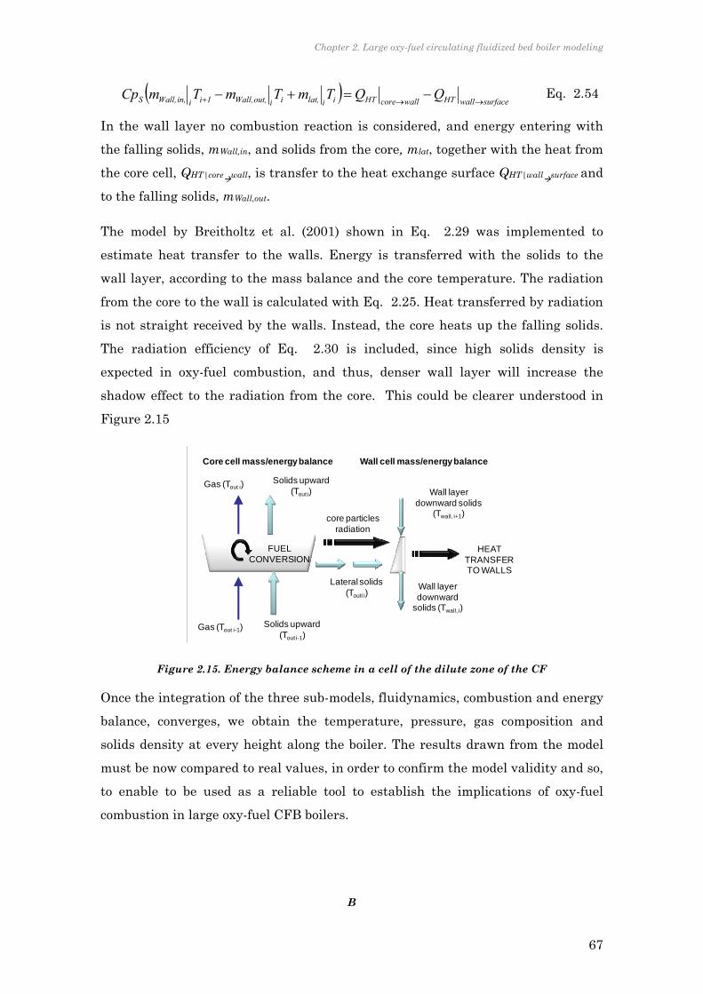
Chapter 2. Large oxy-fuel circulating fluidized bed boiler modeling
67
surfacewallHTwallcoreHTiilat,iiout, Wall,1iiin, Wall,S QQTmTmTmCp
Eq. 2.54
In the wall layer no combustion reaction is considered, and energy entering with
the falling solids, mWall,in, and solids from the core, mlat, together with the heat from
the core cell, QHT|corewall, is transfer to the heat exchange surface QHT|wallsurface and
to the falling solids, mWall,out.
The model by Breitholtz et al. (2001) shown in Eq. 2.29 was implemented to
estimate heat transfer to the walls. Energy is transferred with the solids to the
wall layer, according to the mass balance and the core temperature. The radiation
from the core to the wall is calculated with Eq. 2.25. Heat transferred by radiation
is not straight received by the walls. Instead, the core heats up the falling solids.
The radiation efficiency of Eq. 2.30 is included, since high solids density is
expected in oxy-fuel combustion, and thus, denser wall layer will increase the
shadow effect to the radiation from the core. This could be clearer understood in
Figure 2.15
Figure 2.15. Energy balance scheme in a cell of the dilute zone of the CF
Once the integration of the three sub-models, fluidynamics, combustion and energy
balance, converges, we obtain the temperature, pressure, gas composition and
solids density at every height along the boiler. The results drawn from the model
must be now compared to real values, in order to confirm the model validity and so,
to enable to be used as a reliable tool to establish the implications of oxy-fuel
combustion in large oxy-fuel CFB boilers.
B
FUEL CONVERSION
Solids upward (Tout i-1)
Solids upward (Tout i)
Gas (Tout i-1)
Gas (Tout i)
Wall layer downward
solids (Twall, i)
Wall layer downward solids
(Twall, i+1)
Lateral solids (Touti i)
HEAT TRANSFER TO WALLS
Core cell mass/energy balance Wall cell mass/energy balance
core particles radiation

2.4. Model validation
68
2.4 MODEL VALIDATION
2.4.1 AIR FIRING
In spite of the scarce published data on commercial and large-scale fluidized bed
boilers, some published measurements could be useful for confirming the model
feasibility and reliability:
Published data Author
Pressure drop profile Yang et al. (2005)
Flue gas composition Lee and Kim (1999)
Temperature profile Hannaes et al. (1995)
The measurements published by Yang et al. (2005) has been taken as a reference
for comparing pressure drop along the boiler. The 135We CFB boiler, located at
Zibo power station was 38 m height, and the cross section was 6.6 x 13.1 m2. They
specified the coal used in the plant, that contained 45.39% of fixed carbon, 4.44%
moisture and 16.73% of volatile matter. The heating value was 21060 kJ/kg. Some
of the operation conditions at which measurements were taken were indicated. A
temperature of 885ºC in one case and 896ºC in the other was average along the
riser. Elutriated solids were 5.79 and 6.50 kg/m2s respectively. With these inputs,
comparison of measurements and model are shown in Figure 2.16.
Figure 2.16. Comparison of model pressure profile prediction with the one reported in Yang et al. (2005)

Chapter 2. Large oxy-fuel circulating fluidized bed boiler modeling
69
From the Figure 2.16 it can be confirmed that realistic values of pressure drop
profile are drawn from the model.
For main gas species concentration in the boiler, emissions of CO2 and O2, are
reported by Lee and Kim (1999) and Hannaes et al. (1995), for a 200 and 120 MW
boiler respectively. The former was a 32 m height CFB with a cross section of 19 m
7m. The coal used is a Korean Anthracite with 53.7% fixed carbon and only 4% of
volatile matter and 3.3% moisture. Average temperature was 900ºC. Entering said
parameters, comparison results are shown in Figure 2.17.
Figure 2.17. Comparison of flue gas composition prediction with the one reported in Lee and Kim (1999)
Figure 2.17 cannot be considered a proper validation, since measurements of the
gas composition along the height of the riser were not available and the deviation
of CO2 and O2 results is usually small, even for the simplest modelling approach.
Even though, the common available data from real boilers are taken at the flue gas
outlet. Figure 2.17 is also interesting for showing the estimated CO2 and O2 profile
by the model. It shows the reducing zone commented in the section 2.3.2 and it can
be also distinguished that most of the combustion reactions take place in the lower
zone of the boiler.
Temperature profile measurements in a 120 MW boiler was reported by Hannaes
et al. (1995), for validating the IEA-CFB model. The boiler is 30 m height and 38
m2 in cross section. However, they do not specify the coal used in the tests, so a
bituminous coal was assumed, with a fix coal fraction of 63%, 5.7% moisture and
24% volatile, and 24450 kJ/kg as heating value.
0%
5%
10%
15%
20%
25%
0 5 10 15 20 25 30 35
Volume fraction (%
)
Height (m)
O2 Exp (Lee 1999) CO2 Exp (Lee 1999) O2 model CO2 model

2.4. Model validation
70
Figure 2.18. Comparison of the model temperature profile result with the one reported in Hannaes et al. (1995)
In Figure 2.18 the two highest thermocouples indicated a drastic decrease of
temperature. The reason was the additional heat exchanger tubes located at this
point. Solids at this location were then further cooled.
In general, the model developed in this work gives reliable results. It can be
adapted to different input conditions, satisfactorily estimating the measurements
from large scale boilers. More accurate predictions could be achieved, particularly
with a more detailed combustion modelling. However, for the aim of this work, the
model is more useful if it can be flexible for different configurations and inputs
parameters.
2.4.2 OXY-FIRING
Since there is no available data from commercial CFB installations operating
under oxy-firing conditions, the validation for these cases is based on a
quantitative comparison of published simulations (Nsakala et al., 2004;
Saastamoinen et al., 2006; Seddighi et al., 2010)
In order to validate the present model, heat transfer ratio per fuel input in the
different heat transfer locations will be compared. Three main zones are
distinguished in the the CFB system: furnace walls, including water walls and
wing walls; external heat exchanger (EHE) in the loop-seals, for cooling down
recycled particles before re-injected to the boiler; and the energy contained in the
flue gas stream.
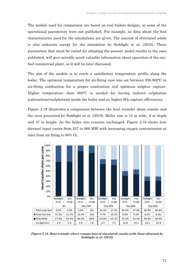
Chapter 2. Large oxy-fuel circulating fluidized bed boiler modeling
71
The models used for comparison are based on real boilers designs, so some of the
operational parameters were not published. For example, no data about the fuel
characteristics used for the simulations are given. The amount of elutriated solids
is also unknown except for the simulation by Seddighi et al. (2010). These
parameters that must be varied for adapting the present model results to the ones
published, will give actually much valuable information about operation of the oxy-
fuel commercial plant, as it will be later discussed.
The aim of the models is to reach a satisfactory temperature profile along the
boiler. The optimum temperature for air-firing case was set between 850-900ºC in
air-firing combustion for a proper combustion and optimum sulphur capture.
Higher temperature than 900ºC is needed for having indirect sulphation
(calcinations+sulphation) inside the boiler and so, higher SO2 capture efficiencies.
Figure 2.19 illustrates a comparison between the heat transfer share results and
the ones presented by Seddighi et al. (2010). Boiler size is 15 m wide, 6 m depth
and 37 m height. As the boiler size remains unchanged, Figure 2.19 shows how
thermal input varies from 257 to 900 MW with increasing oxygen concentration at
inlet from air firing to 80% O2.
Figure 2.19. Heat transfer share comparison of simulated results with those obtained by Seddighi et al. (2010)
Seddighi et al.
this study
Seddighi et al.
this study
Seddighi et al.
this study
Seddighi et al.
this study
Seddighi et al.
this study
Air Oxy 24% Oxy 40% Oxy 60% Oxy 80%
Rate Loop Seal 0.0% 0.0% 0.0% 0% 26.5% 27.5% 49.9% 47.0% 60.8% 60.8%
Rate Flue Gas 31.9% 31.5% 10.5% 14% 9.7% 10.5% 8.9% 9.6% 8.4% 8.3%
Rate Walls 67.8% 68.5% 89.5% 86% 63.9% 62.1% 41.3% 43.4% 30.8% 30.9%
Gs (kg/m2s) 1.9 2.4 1.9 7.8 5.2 7.0 14.8 14.2 24.2 22.4
0%
10%
20%
30%
40%
50%
60%
70%
80%
90%
100%
Heat transfer share per zone
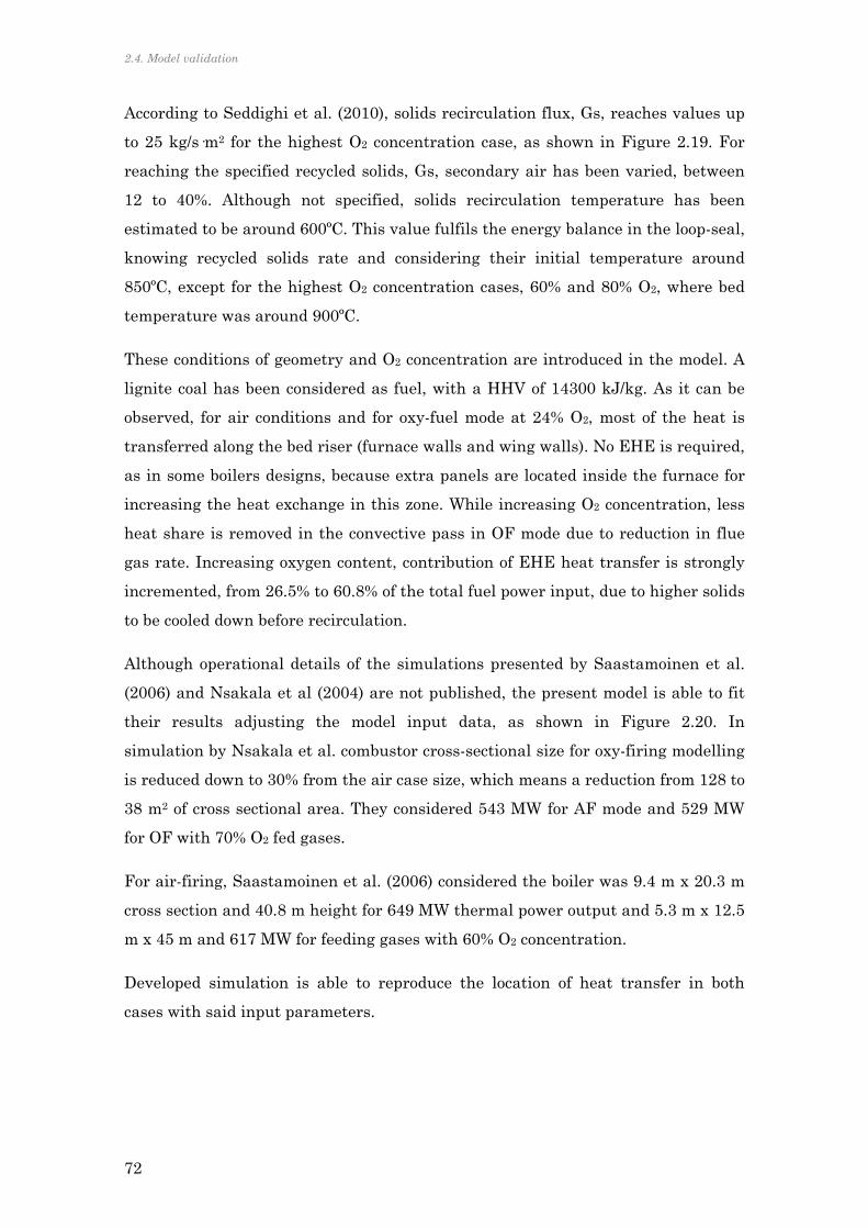
2.4. Model validation
72
According to Seddighi et al. (2010), solids recirculation flux, Gs, reaches values up
to 25 kg/s·m2 for the highest O2 concentration case, as shown in Figure 2.19. For
reaching the specified recycled solids, Gs, secondary air has been varied, between
12 to 40%. Although not specified, solids recirculation temperature has been
estimated to be around 600ºC. This value fulfils the energy balance in the loop-seal,
knowing recycled solids rate and considering their initial temperature around
850ºC, except for the highest O2 concentration cases, 60% and 80% O2, where bed
temperature was around 900ºC.
These conditions of geometry and O2 concentration are introduced in the model. A
lignite coal has been considered as fuel, with a HHV of 14300 kJ/kg. As it can be
observed, for air conditions and for oxy-fuel mode at 24% O2, most of the heat is
transferred along the bed riser (furnace walls and wing walls). No EHE is required,
as in some boilers designs, because extra panels are located inside the furnace for
increasing the heat exchange in this zone. While increasing O2 concentration, less
heat share is removed in the convective pass in OF mode due to reduction in flue
gas rate. Increasing oxygen content, contribution of EHE heat transfer is strongly
incremented, from 26.5% to 60.8% of the total fuel power input, due to higher solids
to be cooled down before recirculation.
Although operational details of the simulations presented by Saastamoinen et al.
(2006) and Nsakala et al (2004) are not published, the present model is able to fit
their results adjusting the model input data, as shown in Figure 2.20. In
simulation by Nsakala et al. combustor cross-sectional size for oxy-firing modelling
is reduced down to 30% from the air case size, which means a reduction from 128 to
38 m2 of cross sectional area. They considered 543 MW for AF mode and 529 MW
for OF with 70% O2 fed gases.
For air-firing, Saastamoinen et al. (2006) considered the boiler was 9.4 m x 20.3 m
cross section and 40.8 m height for 649 MW thermal power output and 5.3 m x 12.5
m x 45 m and 617 MW for feeding gases with 60% O2 concentration.
Developed simulation is able to reproduce the location of heat transfer in both
cases with said input parameters.
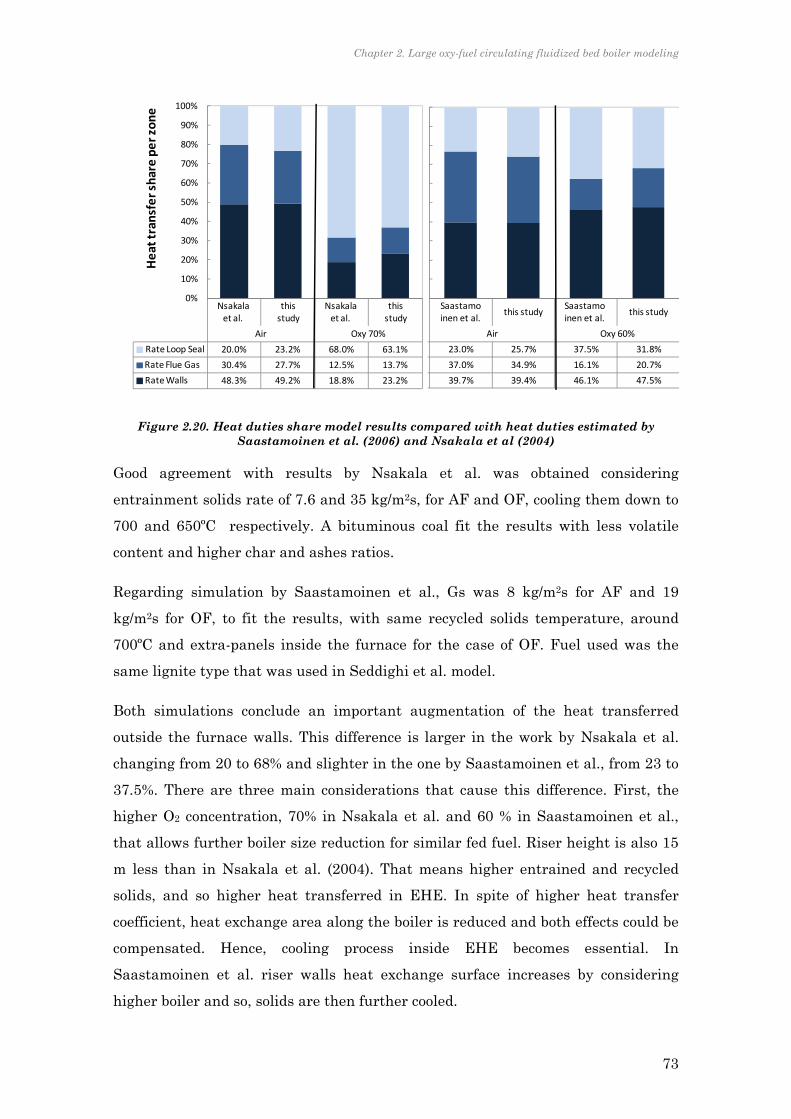
Chapter 2. Large oxy-fuel circulating fluidized bed boiler modeling
73
Figure 2.20. Heat duties share model results compared with heat duties estimated by Saastamoinen et al. (2006) and Nsakala et al (2004)
Good agreement with results by Nsakala et al. was obtained considering
entrainment solids rate of 7.6 and 35 kg/m2s, for AF and OF, cooling them down to
700 and 650ºC respectively. A bituminous coal fit the results with less volatile
content and higher char and ashes ratios.
Regarding simulation by Saastamoinen et al., Gs was 8 kg/m2s for AF and 19
kg/m2s for OF, to fit the results, with same recycled solids temperature, around
700ºC and extra-panels inside the furnace for the case of OF. Fuel used was the
same lignite type that was used in Seddighi et al. model.
Both simulations conclude an important augmentation of the heat transferred
outside the furnace walls. This difference is larger in the work by Nsakala et al.
changing from 20 to 68% and slighter in the one by Saastamoinen et al., from 23 to
37.5%. There are three main considerations that cause this difference. First, the
higher O2 concentration, 70% in Nsakala et al. and 60 % in Saastamoinen et al.,
that allows further boiler size reduction for similar fed fuel. Riser height is also 15
m less than in Nsakala et al. (2004). That means higher entrained and recycled
solids, and so higher heat transferred in EHE. In spite of higher heat transfer
coefficient, heat exchange area along the boiler is reduced and both effects could be
compensated. Hence, cooling process inside EHE becomes essential. In
Saastamoinen et al. riser walls heat exchange surface increases by considering
higher boiler and so, solids are then further cooled.
Saastamoinen et al.
this studySaastamoinen et al.
this study
Air Oxy 60%
Rate Loop Seal 23.0% 25.7% 37.5% 31.8%
Rate Flue Gas 37.0% 34.9% 16.1% 20.7%
Rate Walls 39.7% 39.4% 46.1% 47.5%
0%
10%
20%
30%
40%
50%
60%
70%
80%
90%
100%
Heat transfer share per zone
Nsakala et al.
this study
Nsakala et al.
this study
Air Oxy 70%
Rate Loop Seal 20.0% 23.2% 68.0% 63.1%
Rate Flue Gas 30.4% 27.7% 12.5% 13.7%
Rate Walls 48.3% 49.2% 18.8% 23.2%
0%
10%
20%
30%
40%
50%
60%
70%
80%
90%
100%
Heat transfer share per zone

2.5. The role of the external heat exchanger
74
In the model by Seddighi et al. (2010), boiler size was not modified and bed
temperature was controlled by increasing the amount of recycled solids. Heat
removed in the convective pass during oxy-fuel simulations represent 8-10% of the
total thermal power fed and does not change significantly varying O2 concentration
at inlet. If gas flow rate per fuel input does not vary significantly and boiler
temperatures keep similar, shared of heat that can be extracted by gas convection
per unit fuel input is also similar within different oxy-fuel conditions.
2.5 THE ROLE OF THE EXTERNAL HEAT EXCHANGER
2.5.1 REDUCTION OF OXY-FUEL BOILER SIZE
New OF CFB boiler designs, using high O2 concentrations in the oxidant stream,
may lead to reduce boiler size and so, capital costs. This means also diminishing
the mass flow of gas per unit of thermal fuel input. This will allow reducing the
cross sectional area for reaching similar fluidizing velocities. However, decreasing
the boiler cross sectional area involves a considerable reduction on the available
area along the riser for heat exchange in the wall tubes.
The OF CFB model is used to estimate the consequences of the boiler size
reduction. With this aim, four runs results are compared in , the AF case and three
OF cases, at three O2 concentrations. Fuel input is kept constant, at 650 MW,
feeding low rank Spanish lignite. Temperature at which elutriated solids are
recycled back into the boiler is 700ºC. The heat share called Rate Loop Seal is
calculated by the elutriated solids and the energy difference between the bed
temperature and the imposed recycled temperature. Average bed temperature is
between 850ºC and 900ºC in all the cases. Fixing these parameters will allow
isolating the effect of increasing O2 at inlet, for a certain thermal power.
For fixed boiler geometry, AF case and 30% O2 case require similar recycled solids
rate, to lie within the appropriate bed temperature range, Figure 2.21. Energy
contained in flue gases is lower in the case of OF than AF due to the change in gas
flow rate. This is, O2 concentration is higher in OF 30% than in AF (21%) so the
mass flow of gas conveys less energy than in AF. This difference is distributed in
an increment of 2 points on the EHE and 3 points in the walls. The increment in

Chapter 2. Large oxy-fuel circulating fluidized bed boiler modeling
75
the wall region is due to an increase in bed temperature around 40 ºC compared
with the AF bed temperature.
Figure 2.21. Heat transfer share for different oxygen concentration, 650 MW power input
In the two other OF cases the O2 concentration is incremented up to 45% and 60%
respectively. This is to acquire an estimation of the increase of elutriated solids
needed for controlling bed temperature and hence, the higher heat that the EHE
must remove. The elutriated solids must augment up to 11 and 25 kg/m2s
respectively. Energy with gases almost halves the flue gases heat share in AF. As a
consequence, the heat removed in the EHE is almost double. The cross sectional
area for the 60% O2 case is reduced to 34% from the original size. This also
contributes to diminish the cooling capacity of the riser water walls 7%.
2.5.2 VARYING POWER INPUT
The flexibility that fluidized beds exhibit for working under different fuel loads
resides on the possibility of reducing or increasing elutriated solids, Gs, for
regulating the bed temperature. This can be a particular great advantage for OF
combustion if an appropriately flexible EHE is available. Broad variety of thermal
power output in the same boiler can be handled in a OF CFB. With the aim of
Air Oxy 30% Oxy 45% Oxy 60%
Rate Loop Seal 23.27% 25.34% 40.04% 48.76%
Rate Flue Gas 34.86% 30.82% 22.28% 17.91%
Rate Walls 40.68% 43.84% 37.69% 33.33%
Gs (kg/m2s) 7.8 7.8 18.5 32.7
A cross (m2) 190.8 190.8 103.4 64.0
0%
10%
20%
30%
40%
50%
60%
70%
80%
90%
100%Heat transfer share per zone
2.5. The role of the external heat exchanger
76
understanding this particular feature, a certain boiler size was fixed and the boiler
geometry was selected, with a cross section of 12.5 m x 5.3 m and 40 m high. In the
simulations results are shown in Figure 2.22. Oxygen concentration of 60% at inlet
and solids are recycled at 700ºC were the input values in these runs.
Figure 2.22. Heat transfer share for three fuel inputs and same boiler geometry
While increasing fuel input and so, the required stoichiometric O2, the fluidizing
gas is incremented. To achieve the adequate rate of Gs that made possible a proper
regulation of bed temperature, between 850 and 900ºC, the secondary gas ratio, per
total fed gas is manipulated. By increasing this ratio, the primary gas, and so, the
fluidizing velocity, is controlled within the convenient limits to convey the proper
amount of solids out o the boiler.
As observed in Figure 2.22, an increment of 200 MW in the fuel, means that more
than double of the necessary combustion gas should be deviated, not being fed in
the lower part of the boiler. If this deviation were not enough, the high fluidizing
velocity would drag too many solids and thus, the bed would be cooled down below
the acceptable limits.
In the runs results shown in Figure 2.22, fuel input from 600 to 800 MW, needs Gs
ranging from 25 to 40 kg/m2s, thanks to secondary air ratio, that was varied from
600 MW 700 MW 800 MW
Rate Loop Seal 42.28% 48.28% 52.77%
Rate Flue Gas 17.22% 18.04% 18.16%
Rate Walls 40.00% 33.68% 29.07%
Gs (kg/m2s) 25.4 32.3 39.7
Sec Gas 20% 34% 43%
0%
10%
20%
30%
40%
50%
60%
70%
80%
90%
100%
Heat transfer share per zone
Chapter 2. Large oxy-fuel circulating fluidized bed boiler modeling
77
20-43%. In spite of keeping temperature difference between the bed and the
recycled solids similar in all cases, the increase of Gs makes the contribution of the
EHE increments from 42.3 to 52.8%.
2.5.3 VARYING O2 AT INLET
The distinguishing characteristic of OF combustion versus AF combustion lies on
the possibility of modifying the O2 content in the fluidizing gas. While in AF, the
only way of changing fluidizing velocity is by incrementing the air excess, in OF
case, it also can be varied by manipulating the O2 concentration at inlet.
In future concepts of OF CFB boilers it will be essential to know what flexibility is
possible to achieve for a certain boiler arrangement similar to AF case. In the
following runs an area of 16 x 9.4 m was considered, as the adequate size for air
firing boilers.
Reaching AF temperature conditions is possible with an O2 concentration around a
30% v. This statement has been extensively assumed for pulverized fuel boilers
(Scheffknecht, 2009) but fluidized bed do not present such a great restriction in
feeding wider range of O2 concentration.
A proper temperature profile along the furnace is possible for higher O2
concentrations, when fuel input is also increased. Therefore, higher volume of
gases must be introduced into the boiler and so, higher velocity entrains more
solids to the particles separator device (cyclone).
Figure 2.23 shows the distribution of heat transfer along the system, for keeping
similar temperature profile in the boiler, but different conditions of the oxidant
stream.

2.5. The role of the external heat exchanger
78
Figure 2.23. Heat transfer share with air design boiler geometry and different O2 concentrations at inlet
When O2 at inlet is incremented up to 40%, it is possible to raise entrainment of
solids, up to 20.7 kg/m2s. More particles are managed by the EHE and so 36.7% of
the total fuel input is removed in this part. But it is also possible to maintain the
fluid-dynamical conditions by increasing the temperature difference of solids that
comes out from the boiler. In the last column of Figure 2.23, Gs has been kept
similar than in the 30% O2 case, but solids have been cooled down to 620ºC. Hence,
the contribution of EHE represents 35% of the overall fuel input, as high as the
case of high Gs. In these runs, geometry has been kept constant, but Gs changes by
varying fuel input, up to 730 MW. From the graph it is found that the possibilities
of proper regulation of the fluidized bed operation fall on the external device for
cooling down the particles that are coming back into the boiler. It is possible to
recycle larger amount of solids, or to cool them down to lower recycled
temperatures. In both cases, an important effort must be dedicated to a proper
external heat exchanger design. Conventionally, EHE devices for CFB are bubbling
fluidized beds or moving fluidized beds.
Air Oxy 30% Oxy 40% Oxy 40%
Rate Loop Seal 21.83% 24.61% 37.73% 40.80%
Rate Flue Gas 35.82% 31.94% 25.39% 23.98%
Rate Walls 42.36% 43.46% 36.68% 35.22%
Gs (kg/m2s) 11.0 11.2 20.7 10.6
Fuel input (MW) 570 580 850 730
0%
10%
20%
30%
40%
50%
60%
70%
80%
90%
100%Heat transfer share per zone Trecirc = 720ºC Trecirc = 620ºC
Chapter 2. Large oxy-fuel circulating fluidized bed boiler modeling
79
2.6 CONCLUSIONS
Two of the models of large-scale oxy-fuel CFB available in open literature have
been developed by boiler companies, with long experience on air-firing large CFB.
These models are presumably complex, and based on computational fluid-dynamics
modeling, although modeling data are not public. In spite of this lack of details, the
one-dimensional modeling developed up to here is able to predict the oxy-fuel boiler
heat balance with similar results as those previously mentioned. The heat balance
has been then compared using the heat ratios, dividing the overall energy balance
into three shares: the energy removed by the walls, the flue gas sensible heat
through the convective pass, and the heat removed in the external heat exchanger,
the three of them, represented by unit of fuel input. The values obtained from the
comparison made the model fairly reliable to be used for further analysis.
The effect of changing O2 concentration on the design of certain boiler geometry
was evaluated. Fixing the fuel input and the temperature at which solids are
recycled, three different O2 concentrations were run. The results indicated that a
much compact boiler is required for the case of 60% O2. For this case, the boiler
cross sectional area was 33% less than the case of 30% O2. This implied a reduction
in the available surface for heat removal in the water walls. Consequently, the heat
transferred in the EHE increased twice from the 30% O2, to the 60% O2 cases.
When boiler geometry was not variable, fuel input did increase for higher O2
percentages, to reach the proper fluidizing velocity. Again, this led to higher heat
removal requirements in the EHE up to 53% from the overall combustion heat.
Oxy-fuel applied in the CFB boiler presents outstanding operating flexibility, for a
range of O2 at inlet, analogous to the conventional case in which boiler load must
change for adapting the energy market requirements.
On the other hand, the EHE is now an essential device for acquiring the mentioned
flexibility and it will not be possible to disregard it in future oxy-fuel CFB boilers
designs.
There will be then two essential differences in the operation between EHE
attached to an oxy-fuel and an air-fired CFB. On the one hand, the fluidizing gas
composition cannot be air, but it will consist of flue gases bleeding, in order to
preserve the purity of the CO2 concentrated flue gas, within acceptable limits for

2.6. Conclusions
80
transport and storage. On the other hand, higher recycled flow of solids will lead to
non-uniformities along the tubes in the EHE. Consequently, the average heat
transfer coefficient will be affected. Following, both issues will be experimentally
assessed and discussed.

81
CHAPTER 3
HEAT TRANSFER IN CIRCE
EXPERIMENTAL OXY-FUEL COMBUSTION
BUBBLING FLUIDIZED BED
3.1 INTRODUCTION
The particular relevance of higher heat removal in the EHE of an oxy-fuel CFB
leads the attention towards an adequate design of the heat transfer areas and the
allocation of this equipment. EHEs work usually under bubbling regime conditions.
This allows the proper displacement of solids from the bottom of the cyclone leg, to
the recycling pipe. At the same time, low velocity fluidization regime prevents from
excess of gas flow through the dip-leg solids column (Grace et al., 1997). The
bubbling regime exhibits an intense heat transfer from the particles to the heat
tubes, due to the dominant contribution of the particle convection mechanism.
Unlike in conventional EHE, the oxy-fuel CFB’s EHE will not be fluidized with air,
but with RFG. Only one previous experience evaluated heat transfer coefficients
under oxy-fuel fluidized bed conditions (Nsakala et al., 2004). They measured the
heat transfer coefficients in the riser of a CFB, finding no significant differences
with the ones measured under air-firing. In the CFB riser, the radiation
contribution and gas convection prevails over the particle convection mechanism,
unlike in dense beds. Thus, presumably, most researchers assume that the change
on the gaseous atmosphere would not mean a significant difference on heat
transfer. However, the change on gas composition would affect the conductivity and
heat capacity of the gas layer adjacent to the wall. This gas layer is, in fact, the
limiting actor to the heat flow. The fluid-dynamics is also assumed to behave
similarly in OF than in AF mode by most of researchers, although the bubbles were

3.2. Heat transfer in fluidized beds
82
found to be slightly smaller and with more vigorous bubbling than in air-firing case
(Guedea et al., 2011). This affects the fraction of time during which particles are in
contact with the surface.
Heat transfer in an oxy-fuel bubbling fluidized bed (BFB) is measured in this work.
This will allow evaluating the differences with the known air-combustion
operation. The two main approaches used for the prediction of heat transfer
coefficients in fluidized beds, the empirical and the mechanistic approaches, are
examined to forecast the differences between air and oxy-fuel operation. The heat
transfer coefficients measured during the pilot plant operation will allow proposing
a complete expression for the heat transfer coefficient during oxy-fuel combustion
in fluidized beds.
3.2 HEAT TRANSFER IN FLUIDIZED BEDS
3.2.1 PREVIOUS FINDINGS
Heat transfer between a surface and a gas flowing through a bed of particles is
many times higher than expected for the same flow in an empty column. Thus, the
heat transferred through particles in movement is rather more intense than the
gas convection alone. Heat from hot particles to the cold inlet fluidization gas is
transferred intensively. Thus, bed and gas temperatures are generally considered
equal to the average bed temperature, even in the vicinity of the distributor.
Researchers confirmed this phenomenon and it was mostly represented by means
of empirical expressions. Compendium of correlations of heat transfer between gas
and solid particles in fluidized beds can be found in general literature of fluidized
beds like (Botterill, 1989; Howard, 1989; Kunii and Levenspiel, 1991; Oka, 2003;
Basu, 2006). Although these quantification is particularly relevant for the modeling
of fuel particle conversion, in this work the heat transfer from the particles to the
gas will be considered high enough to be neglected.
The mechanisms involved in the heat transfer between the bed and the surface
include:
‐ The solid conduction that takes place while solid particles contact the
surface. The emulsion phase contains the majority of solid particles, but

Chapter 3. Heat transfer in CIRCE experimental oxy-fuel combustion bubbling fluidized bed
83
there is also a small proportion in the bubble phase. Although it is based on
solids conduction, this mechanism is known as particle convection, because
the movement of solids greatly enhances the energy transfer, hpc.
‐ The gas convection from both, the bubble phase and the gas found in the
emulsion, hgc.
‐ The radiation heat transfer from the layer adjacent to the wall, hrad.
As an engineering approximation the contribution of these mechanisms are
regarded as independent, from each other, and the heat transfer coefficient is then
written as:
rpcgc hhhh Eq. 3.1
The particle convection heat transfer mechanism prevails in fluidized bed region
for bubbling fluidized beds and in the freeboard, radiation mechanism dominates.
Thus, heat transfer coefficients to immersed surfaces in the fluidized region can
range from 250 to 700 W/m2K and in the freeboard these coefficients are less than
100 W/m2K (Breitholtz et al., 2001; Oka, 2003). The transition in the heat transfer
values in the splash zone was measured by Pidwerbecki and Wely (1995).
Moreover, radiation heat transfer is often neglected when the bed temperature is
lower than 600ºC. Numerous authors analyzed the parameters influencing heat
transfer at low temperature, isolating the radiation contribution. In most of cases,
the cooling rate of a heated surface (van Heerden et al., 1953; Ziegler et al., 1964;
Schmidt and Renz, 2005; Patil et al., 2006) or sample probe (Grewal and Saxena,
1981; Mathur et al., 1986; Sunderesan and Clark, 1995) is used to measure the
energy transfer. Since the earliest studies it was stated that the greatest influence
on heat transfer intensity is that of the fluidization velocity and particle size:
On the one hand, fluidizing velocity influence is usually described in three stages:
‐ At fixed bed regime, heat is transferred by conduction of particles in contact
with the surface and by convective gas flow between bed particles. With
onset of fluidization, particle convection heat transfer starts. At minimum
fluidization velocity, heat transfer increases sharply.
‐ With further increase in fluidization velocity, heat transfer coefficient
continues to increase, and it reaches a maximum at an optimal fluidization
velocity. Below this limit, the major contributor to heat transfer is the
particle convection, increasing with particle mixing.

3.2. Heat transfer in fluidized beds
84
‐ With velocities higher than the optimal velocity, the key mechanism of heat
transfer is gas convection. Since bed density is lower, the influence of
particle convection decreases.
Particle size, on the other side, determines the relative influence of each
mechanism. With increasing particle diameter, optimal fluidization velocity
increases and the maximum heat transfer coefficient is significantly smaller. In
fluidized beds of small particles less than 0.1 mm, particle convection makes for
more than 90% of heat transfer, while in beds with particles greater than 1 mm, it
makes only 20% of particle heat transfer. A detailed review of the influence of
particle diameter on heat transfer can be found in Decker and Glicksman (1983).
The role of gas convection becomes significant when the gas flow occurs at particle
diameters greater than about 800 μm. For particles of this size and larger, the
convective component of heat transfer by gas becomes significant and total heat
transfer coefficient does not depend much on the particle size.
Additionally, the solids density is closely related to both, the fluidizing velocity and
the particle size. Breitholtz et al. (2001) gathered experimental data from pilot and
large plants, and established a simple correlation that directly related the global
heat transfer coefficient with the solids suspension density. Their study focused on
circulating fluidized bed boilers, but they highlighted the adequacy of bed density
for satisfactorily predict the heat transfer coefficients in a generalized way.
Empirical approaches
One of the most widely recommended expressions for estimating heat transfer in
fluidized beds is the one proposed by Zabrodsky (1966). Due to simplicity and also,
the reasonable predictions given, it has been extensively used along decades
(Botterill, 1989; Howard, 1989; Basu, 2006).
0.36p
0.6g
0.2
g
smax dk
ρ
ρ37.6h
Eq. 3.2
Note that the energy units for this expression were not S.I. but kcal/h. Botterill et
al. (1984) recommended that a value of about 70% of that predicted by Eq. 3.1
represents a conservative estimate for hmax.
Earlier common approaches for modeling heat transfer to surfaces in fluidized beds
assumed similarity to gaseous convection and assigned thermal resistance to a
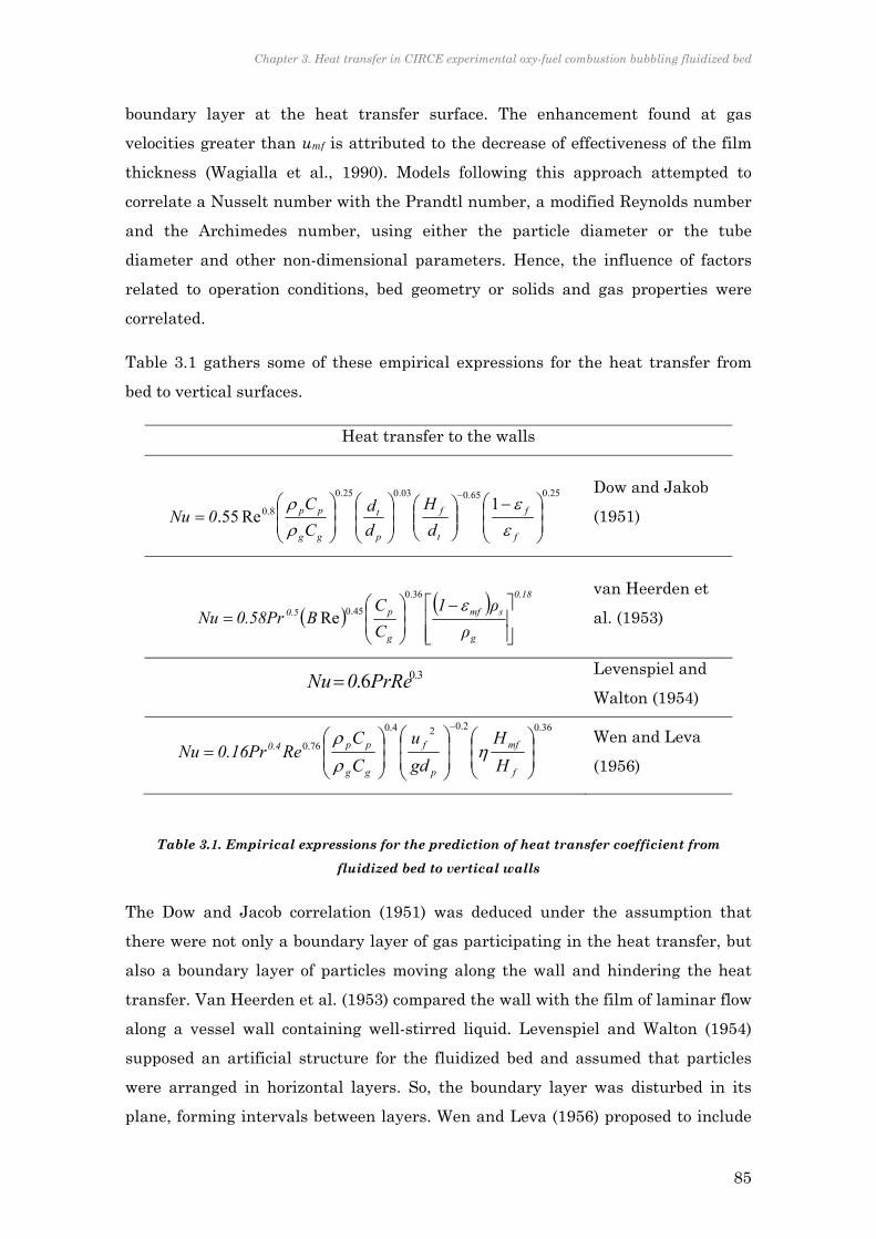
Chapter 3. Heat transfer in CIRCE experimental oxy-fuel combustion bubbling fluidized bed
85
boundary layer at the heat transfer surface. The enhancement found at gas
velocities greater than umf is attributed to the decrease of effectiveness of the film
thickness (Wagialla et al., 1990). Models following this approach attempted to
correlate a Nusselt number with the Prandtl number, a modified Reynolds number
and the Archimedes number, using either the particle diameter or the tube
diameter and other non-dimensional parameters. Hence, the influence of factors
related to operation conditions, bed geometry or solids and gas properties were
correlated.
Table 3.1 gathers some of these empirical expressions for the heat transfer from
bed to vertical surfaces.
Heat transfer to the walls
25.065.003.025.0
8.0 1Re55.
f
f
t
f
p
t
gg
pp
d
H
d
d
C
C0Nu
Dow and Jakob
(1951)
0.18
g
smf
g
p0.5
ρ
ρ1
C
CB0.58PrNu
36.0
45.0Re
van Heerden et
al. (1953)
3.06. PrRe0Nu Levenspiel and
Walton (1954)
36.02.024.0
76.0
f
mf
p
f
gg
pp0.4
H
H
gd
u
C
CRe0.16PrNu
Wen and Leva
(1956)
Table 3.1. Empirical expressions for the prediction of heat transfer coefficient from
fluidized bed to vertical walls
The Dow and Jacob correlation (1951) was deduced under the assumption that
there were not only a boundary layer of gas participating in the heat transfer, but
also a boundary layer of particles moving along the wall and hindering the heat
transfer. Van Heerden et al. (1953) compared the wall with the film of laminar flow
along a vessel wall containing well-stirred liquid. Levenspiel and Walton (1954)
supposed an artificial structure for the fluidized bed and assumed that particles
were arranged in horizontal layers. So, the boundary layer was disturbed in its
plane, forming intervals between layers. Wen and Leva (1956) proposed to include
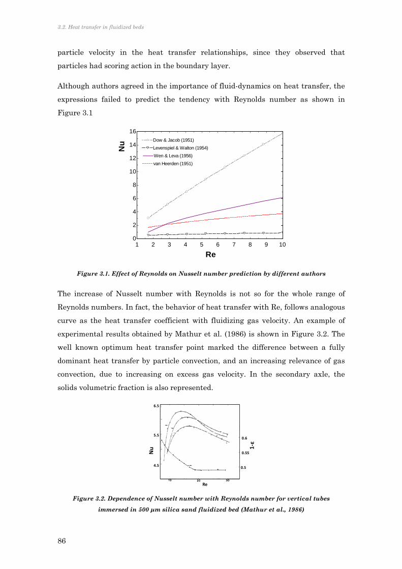
3.2. Heat transfer in fluidized beds
86
particle velocity in the heat transfer relationships, since they observed that
particles had scoring action in the boundary layer.
Although authors agreed in the importance of fluid-dynamics on heat transfer, the
expressions failed to predict the tendency with Reynolds number as shown in
Figure 3.1
Figure 3.1. Effect of Reynolds on Nusselt number prediction by different authors
The increase of Nusselt number with Reynolds is not so for the whole range of
Reynolds numbers. In fact, the behavior of heat transfer with Re, follows analogous
curve as the heat transfer coefficient with fluidizing gas velocity. An example of
experimental results obtained by Mathur et al. (1986) is shown in Figure 3.2. The
well known optimum heat transfer point marked the difference between a fully
dominant heat transfer by particle convection, and an increasing relevance of gas
convection, due to increasing on excess gas velocity. In the secondary axle, the
solids volumetric fraction is also represented.
Figure 3.2. Dependence of Nusselt number with Reynolds number for vertical tubes
immersed in 500 μm silica sand fluidized bed (Mathur et al., 1986)
1 2 3 4 5 6 7 8 9 100
2
4
6
8
10
12
14
16
Re
Nu Dow & Jacob (1951)Dow & Jacob (1951)
Levenspiel & Walton (1954)Levenspiel & Walton (1954)
van Heerden (1951)van Heerden (1951)
Wen & Leva (1956)Wen & Leva (1956)
0.6
0.55
0.5
1‐ε
6.5
5.5
4.5
Nu
Re

Chapter 3. Heat transfer in CIRCE experimental oxy-fuel combustion bubbling fluidized bed
87
Molerus et al. (1994) proposed a new fully empirical correlation, deduced from the
two limiting conditions for heat transfer in fluidized bed: fully dominant gas
convection (105 < Ar < 108) or fully dominant particle convection (Ar < 102).
11
mf
mf
1/3
gp
g1/3
mf
mf
2
mf3
g
pp
0.5
gp
g2mf
p
g
11
mf3
g
pp3
mf
mfmf
g
l
u
uu0.051
ρρ
ρ0.165Pr...
...
uu
uuu
gk
cρ
ρρ
ρε10.281
μ2c
k1
uugk
cρ
u
uu33.31ε10.125
k
hl
Eq. 3.3
Eq. 3.3 was deduced from cold tests, but still, it appears as a quite reliable
expression for predicting the behavior of changes in gas composition, as in oxy-fuel
combustion. The existing expressions were modified to represent the dependence of
heat transfer on the slip velocity parameter. This expression was compared with
numerous experimental data from other authors and agrees in the prediction of the
real tendency of heat transfer with Reynolds number.
Mechanistic approaches
Although there is no universal theory for the mechanisms of heat transfer in
fluidized beds, it is generally accepted that heat transfer in BFB is best explained
by the packet renewal model, developed by Mickley and Fairbanks (1955),
explained and recommended in numerous general studies (Xavier and Davidson,
1985; Chen, 2003; Basu, 2006). They analyzed the simple case of aggregates of
particles, named packets, receiving heat while contacting an isothermal flat
surface. Thus, packets of particles at bulk bed temperature are swept to the heat
transfer surface due to the action of bubbles. They stay in contact with the
exchange surface for a period of time τ and then they are swept back to the bed.
During this time, unsteady state heat transfer takes place between the packet and
the surface. Eq. 3.4 yields the instantaneous heat transfer coefficient:
τπ
cρkh Pap,PaPa
in Eq. 3.4
Where the subscript Pa indicates the packet properties. This concept was
experimentally confirmed by researchers who were able to measure transient
3.2. Heat transfer in fluidized beds
88
variations of particle concentration at heat transfer surfaces, for example, with
surface capacitance sensors with flush mounted electrodes, as Chen et al. (2005).
Techniques such an optical probes (Kurosaki et al., 1995) or pressure fluctuation
measurements (van Ommen and Mudde, 2007) are also used for obtaining
quantitative voidage values. All of them allow to obtain real-time measurements of
fluctuating particle concentration at surfaces in fluidized bed (Werther, 1999).
These experiments confirmed that particle concentration is highly dynamic and
varies dramatically over time. An additional heat transfer resistance to the particle
packet transient conduction was first proposed by Baskakov (1964), considering
that the contact zone is time-independent with changing properties and it could not
be considered as a continuous medium. Particle concentration alternates between
pure gas (bubble phase) and high concentration similar to that for packed beds
(emulsion packet phase). These evidences support the renewal model where the
time average heat transfer coefficient involves proportional contributions from the
bubble phase coefficient and packet phase coefficient (Xavier and Davidson, 1985),
Eq. 3.5:
gcbpcb h)h(1h Eq. 3.5
There are two difficulties added to the evaluation of the transient conduction term.
On the one hand, time-domain parameters are not easy to measure or evaluate.
These parameters include fd, the fraction of time when surface is in contact with
dense phase and τ, the root mean residence time of packets at the heat transfer
surface. According to the two-phase approach for fluid-dynamics in a fluidized bed,
where bubbles as composed by pure gas, the frequency at which solids packets are
contacting the wall is related to the residence time through the bubble fraction δb
as shown in Eq. 3.6:
τ
δ1f-1 b
d
Eq. 3.6
On the other hand, Eq. 3.4 is reasonably accurate for long packet residence times
or very small particle diameters, because it ignores variations in bed voidage with
distance normal to the surface. Thus, physical and thermal properties of packet
near the surface must be estimated as effective properties (Xavier and Davidson,
1985; Kunii and Levenspiel, 1991), taken at one-half of the penetration depth of the
temperature wave for the given operation conditions (Chen, 2003). In 1964
Baskakov modified this model by adding a time-independent contact resistance

Chapter 3. Heat transfer in CIRCE experimental oxy-fuel combustion bubbling fluidized bed
89
between the packed and the surface to account for the zone with variable
properties (Xavier and Davidson, 1985).
Effective thermal conductivity
From the earliest studies on heat transfer (Zabrodsky, 1966), it was observed that
temperature gradient in the proximity of the wall dramatically dropped. This
indicated that the resistance due to the conductivity in the wall layer was more
elevate than the bulk of particles conductivity. The fluidized bed effective thermal
conductivity is higher than the gas or solid particles thermal conductivity. This is
due to the interaction among the particles in bed and the number of contacts
between them and the wall. Furthermore, experiments showed that effective
thermal conductivity in axial directions is one order of magnitude lower than in the
radial direction. This effective conductivity was studied first based on bulk void
fraction and later, on the near-wall void fraction. The importance of accurate
prediction of thermal conductivity has gained importance in the last decade,
thanks to the development of computational fluid-dynamics modeling, which
includes particle-particle interactions in their approaches (Patil et al., 2006; Yusuf
et al., 2012).
Kunii and Levenspiel (1991) proposed Eq. 3.7 to account for the added contribution
to the effective conductivity from the particle through the gas layer and through
the contact point between particles. They corrected the model in which heat would
flow through parallel paths, to account for the geometry of the particles. Based on
analogous approach, Xavier and Davidson (1985) recommended the estimation of
both components of the effective conductivity, as shown in Eq. 3.9. In the equation
it was approximated the solution in packing of spheres and cylinders. The first is
independent of the fluid flow, and second represents the effect of the diffusion in
the fluid phase. Chen et al. (2005) simplified these expressions correlating the
results by other authors in Eq. 3.10.

3.2. Heat transfer in fluidized beds
90
Kunii and
Levenspiel (1991)
3
2k
kφ
1k ε1kεk
g
sb
smfgmfeff
0
3
1k
kφ
1k ε1kεk
g
sw
smfgmfweff
Eq. 3.7
Eq. 3.8
Xavier and
Davidson (1985) mfpgpg
k
k0.057log0.757logε0.28
g
sgeff udc0.1ρ
k
kkk
g
s
Eq. 3.9
Chen et al. (2005)
46.046.0
5.25.3
g
seff k
kk Eq. 3.10
Table 3.2. Effective thermal conductivity of particulate phase by different authors
Figure 3.3 shows the effect of temperature on the effective thermal conductivity,
estimated with Eq. 3.10. The discontinuous line represents the air-firing case and
the oxy-fuel lines are estimated for two O2 concentrations, 40% and 60%. The
effective conductivity during oxy-fuel is higher than in air-firing, and the
temperature influence exhibits similar dominance on this value than the
proportion of O2 in the mixture.
Figure 3.3. Temperature effect on effective thermal conductivity
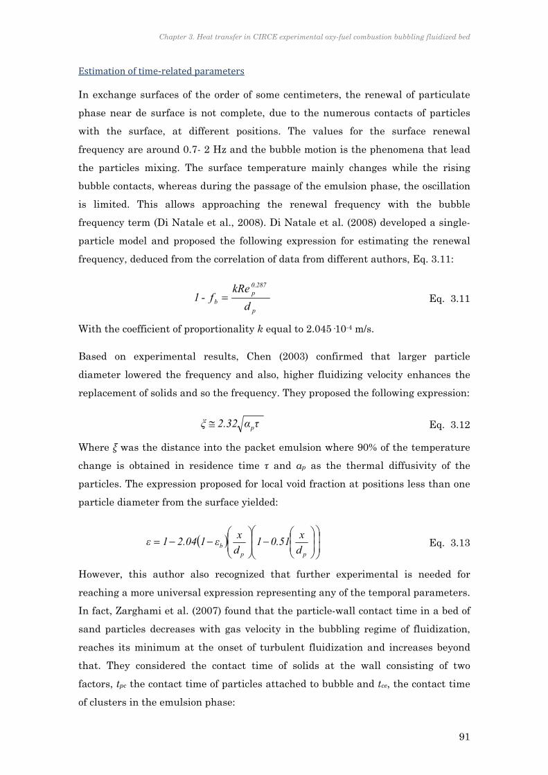
Chapter 3. Heat transfer in CIRCE experimental oxy-fuel combustion bubbling fluidized bed
91
Estimation of time‐related parameters
In exchange surfaces of the order of some centimeters, the renewal of particulate
phase near de surface is not complete, due to the numerous contacts of particles
with the surface, at different positions. The values for the surface renewal
frequency are around 0.7- 2 Hz and the bubble motion is the phenomena that lead
the particles mixing. The surface temperature mainly changes while the rising
bubble contacts, whereas during the passage of the emulsion phase, the oscillation
is limited. This allows approaching the renewal frequency with the bubble
frequency term (Di Natale et al., 2008). Di Natale et al. (2008) developed a single-
particle model and proposed the following expression for estimating the renewal
frequency, deduced from the correlation of data from different authors, Eq. 3.11:
p
0.287p
b d
kRef-1 Eq. 3.11
With the coefficient of proportionality k equal to 2.045·10-4 m/s.
Based on experimental results, Chen (2003) confirmed that larger particle
diameter lowered the frequency and also, higher fluidizing velocity enhances the
replacement of solids and so the frequency. They proposed the following expression:
τα2.32ξ p Eq. 3.12
Where ξ was the distance into the packet emulsion where 90% of the temperature
change is obtained in residence time τ and αp as the thermal diffusivity of the
particles. The expression proposed for local void fraction at positions less than one
particle diameter from the surface yielded:
ppb d
x0.511
d
xε12.041ε Eq. 3.13
However, this author also recognized that further experimental is needed for
reaching a more universal expression representing any of the temporal parameters.
In fact, Zarghami et al. (2007) found that the particle-wall contact time in a bed of
sand particles decreases with gas velocity in the bubbling regime of fluidization,
reaches its minimum at the onset of turbulent fluidization and increases beyond
that. They considered the contact time of solids at the wall consisting of two
factors, tpc the contact time of particles attached to bubble and tce, the contact time
of clusters in the emulsion phase:

3.2. Heat transfer in fluidized beds
92
cepc ttτ Eq. 3.14
The fraction of time in which the surface is bathed by particles attached to bubbles
is proportional to the volume fraction of emulsion in the vicinity of the surface:
bb
be
b
epc uδ
dδa
n
δt Eq. 3.15
Being a an empirical correction factor to take into account the ratio of the existence
probability of bubbles near the surface to their probability within the bed.
For cet it is considered that the clusters are pushed towards the wall by the bubbles
and so, the contact time of the clusters in the emulsion phase is proportional to the
bubble fraction. It is also added a correction factor b for the probability of cluster
being near the surface:
cc
cb
c
bce uδ
dδb
n
δt Eq. 3.16
So, the proposed formula for particle-wall contact time is expressed as:
cc
cb
bb
be uδ
dδb
uδ
dδaτ Eq. 3.17
Factors a and b are correction factors for taking the wall effect into account and so,
evaluating radial distribution of bubbles and cluster. According to their
experiments Zarghami et al. observed less frequently clusters in the wall than in
the center, less frequently bubbles in the center than in the wall. They compared
the experimental results of Hamidipour et al. (2005) with the model developed and
with the expression proposed by Lu et al. (1993):
b
bb
b
d
u3δ
δ12τ
Eq. 3.18
Looking at the influence of slip velocity in residence time, Figure 3.4 illustrates the
prediction by the above-mentioned authors.

Chapter 3. Heat transfer in CIRCE experimental oxy-fuel combustion bubbling fluidized bed
93
Figure 3.4. Predicted residence time dependence on fluidizing velocity, by different authors
The bath shape of Zarghami et al. approach appears a realistic prediction of the
effect of velocity in the residence time of particles. This would agree with the
velocity influence on heat transfer, commented above, in which there would be an
optimal velocity at which residence time were lowest and the packet presence at
the wall had the major importance.
Radiation heat transfer
Radiation heat transfer mechanism begins to contribute appreciably to the overall
heat transfer in bubbling fluidized beds at temperature greater than 500oC.
Measurements of radiant heat transfer in dense beds are scarce. Yamada et al.
(2001) affirmed that the reason was that conclusion from models are contradictory
among authors. In their experiments they showed that the real contribution to this
radiant heat transfer lies on the particles adjacent to the surface, and hinders the
radiation heat transfer between the surface and the higher temperature particles
in the depth of the bed. They measured the influence of particle diameter and
fluidizing velocity on the radiant energy transfer to the surface. In the transport
zone of circulating fluidized beds radiation models are proposed, and extensive
research is available (Luan et al., 2000; Eriksson and Golriz, 2005; Glicksman,
2007). Basu and Konuche (1988) reported that the radiative component is 70%-90%
of the total heat flux transferred from the suspension to the wall at 600ºC-885ºC.
0,5 1 1,5 2 2,50
0,1
0,2
0,3
u - umf (m/s)
(
s)
Chen (2003)
Lu et al. (1993)Lu et al. (1993)
Zarghami et al. (2007)Zarghami et al. (2007)

3.2. Heat transfer in fluidized beds
94
The high percentage of radiation to total heat transfer in CFBs compared with
bubbling fluidized beds is attributed to relatively low convective heat transfer due
to low particle concentrations (Luan et al., 1999).
A simple approach to estimate radiation, used by many authors (Botterill, 1989;
Wirth, 1994; Molerus et al., 1995b; Molerus et al., 1995a; Baskakov and Leckner,
1997; Basu, 2006), is to treat the radiation transfer as the exchange between
opaque gray bodies separated by a nonparticipating medium. Then, the expression
for radiation exchange yields as previously stated in Eq. 2.25. Where, for two
parallel planes much larger than the distance between them, Eq. 2.26 showed the
calculation of the bed-to-wall emissivity. In that expression, the term of bed
emissivity εb is difficult to accurately estimate. It appears that it exceeds the value
of particle emissivity, εp, because of reflections from particles near the bed surface.
This was attributed to the same reason that an irregular surface has a higher
emissivity than a smooth surface of the same material. Effective emissivity of
fluidized bed has been correlated against different bed and wall temperatures and
shown in Botterill (1989). A more simple expression was, however proposed by
Baskakov and Leckner (1997) yielding:
0.64pb εε Eq. 3.19
The heat transfer of the layer of particles near the wall is controlled by a thermal
resistance, Rw. This resistance is determined by the thickness of the gas layer
between the heat transfer surface and the layer of particles. If the value of Rw is
small, particles close to the surface at surface temperature influence is low.
The increase of heat transfer when increasing bed temperature is not only
attributable to radiation heat transfer (Glicksman and Decker, 1982). Gas
conductivity also augments, causing the corresponding increase on conduction
mechanisms. They actually proposed to use an additional radiative conductivity for
including the radiation heat transfer for particles adjacent to the surface. They
added this conductivity term to the effective thermal conductivity and yielded:
3
9
8Tdk pr Eq. 3.20

Chapter 3. Heat transfer in CIRCE experimental oxy-fuel combustion bubbling fluidized bed
95
3.2.2 THEORETICAL INFLUENCES OF OXY-FUEL CONDITIONS
The immediate difference between the air-firing and oxy-firing modes resides on
the atmosphere composition in which combustion and fluidization takes place.
High concentration of CO2, instead of N2 is present in the gases. For acquiring an
impression of how the gas properties would vary in both cases Figure 3.5 shows the
theoretical properties of a mixture of O2/N2 (Air) and a mixture of O2/CO2 at
different O2 proportions, at 850ºC. Density and heat capacity were evaluated as
proportional with gas composition, while conductivity and viscosity follow the
recommendation by Lindsay and Bromley (1950) and Wilke (1950), respectively:
Figure 3.5. Gas properties variation for different O2 concentration at inlet: a) density; b)
viscosity; c) conductivity; d) specific heat capacity
In the four properties observed here, for the same O2 proportion, O2/CO2 mixture
shows higher values. The greatest difference turns out in the gas density, which is
45% higher in the mixture with low O2 compared with O2/N2 mixture. While
increasing O2 in the mixture, the gas density decreases 18%. Heat capacity
diminishes 9 percentage points from the lowest O2 content case, to the highest,
1,12
1,14
1,16
1,18
1,20
1,22
1,24
1,26
0% 20% 40% 60% 80% 100%
c p(kJ/kgK)
O2 (%w.)
O2/N2
0,00
0,05
0,10
0,15
0,20
0,25
0,30
0,35
0,40
0,45
0,50
0% 20% 40% 60% 80% 100%
(kg/m
3 )
O2 (%w.)
O2/N2
O2/CO2
7,2E‐05
7,4E‐05
7,6E‐05
7,8E‐05
8,0E‐05
8,2E‐05
8,4E‐05
0% 20% 40% 60% 80% 100%
k g(kW/m
K)
O2 (%w.)
O2/N2
O2/CO2
4,4E‐05
4,5E‐05
4,6E‐05
4,7E‐05
4,8E‐05
4,9E‐05
5,0E‐05
5,1E‐05
5,2E‐05
0% 20% 40% 60% 80% 100%
(kg/m
s)
O2 (%w.)
O2/N2
O2/CO2
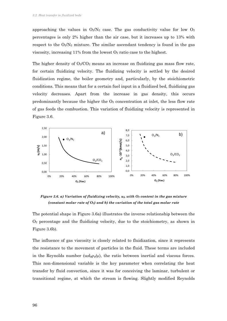
3.2. Heat transfer in fluidized beds
96
approaching the values in O2/N2 case. The gas conductivity value for low O2
percentages is only 2% higher than the air case, but it increases up to 13% with
respect to the O2/N2 mixture. The similar ascendant tendency is found in the gas
viscosity, increasing 11% from the lowest O2 ratio case to the highest.
The higher density of O2/CO2 means an increase on fluidizing gas mass flow rate,
for certain fluidizing velocity. The fluidizing velocity is settled by the desired
fluidization regime, the boiler geometry and, particularly, by the stoichiometric
conditions. This means that for a certain fuel input in a fluidized bed, fluidizing gas
velocity decreases. Apart from the increase in gas density, this occurs
predominantly because the higher the O2 concentration at inlet, the less flow rate
of gas feeds the combustion. This variation of fluidizing velocity is represented in
Figure 3.6.
Figure 3.6. a) Variation of fluidizing velocity, uf, with O2 content in the gas mixture
(constant molar rate of O2) and b) the variation of the total gas molar rate
The potential shape in Figure 3.6a) illustrates the inverse relationship between the
O2 percentage and the fluidizing velocity, due to the stoichiometry, as shown in
Figure 3.6b).
The influence of gas viscosity is closely related to fluidization, since it represents
the resistance to the movement of particles in the fluid. These terms are included
in the Reynolds number (ufdpg/), the ratio between inertial and viscous forces.
This non-dimensional variable is the key parameter when correlating the heat
transfer by fluid convection, since it was for conceiving the laminar, turbulent or
transitional regime, at which the stream is flowing. Slightly modified Reynolds
0,0
1,0
2,0
3,0
4,0
5,0
6,0
7,0
8,0
0% 20% 40% 60% 80% 100%
ng10‐4 (kmol/s)
O2 (%w.)
O2/N2
O2/CO2
0,00
0,50
1,00
1,50
2,00
2,50
0% 20% 40% 60% 80% 100%
uf(m
/s)
O2 (%w.)
O2/N2
O2/CO2
a) b)

Chapter 3. Heat transfer in CIRCE experimental oxy-fuel combustion bubbling fluidized bed
97
number, is used, referred to the particle diameter instead to any longitudinal
parameter.
Archimedes number (dp3g(p-g)/2) also comprises the effect of particle diameter
and solids and gas densities on the fluidization regime (Rabinovich and Kalman,
2011; Shaul et al., 2012). The term of Archimedes number has been usually related
to the contribution of gas convection heat transfer component, like the expressions
used by Kunii and Levenspiel (1991), Xavier and Davidson (1985) or by Botterill et
al. (1989). In circulating fluidized beds the influence of Archimedes number is more
evident. Wirth (1995) established a direct relation between the Archimedes number
and the influence of the gas conductivity in the component of heat transfer by gas.
He stated that, for high Archimedes numbers, the conductivity of gas did not
influence the heat transfer coefficients, unlike for low Archimedes numbers that
based the gas heat transfer on the gas conduction. Archimedes number is also
related to the void fraction of the bed. Void fraction at minimum fluidization
velocity, together with the Archimedes number, are the most influencing
parameters for determining the bed porosity, according to Di Natale et al. (2008).
Thermal properties of gas, such as conductivity and specific heat capacity, are
higher for O2/CO2 mixtures, diminishing with the O2 content in the case of cp.
Prandtl number (cp/kg) includes both variables and reflects the predominant
influence of either convection or conduction heat transfer. This is also a common
parameter participating in forced internal convection correlations. Prandtl varies
slightly for certain gas composition and its value is usually around 0.7 for gaseous
phase.
The influence of gas composition at inlet is now reviewed, by means of non-
dimensional parameters included in Table 3.1. With this aim, Figure 3.7 shows the
influence of gas composition and temperature on the densities ratio, (1-εmf)ρs/ρg, the
Archimedes and Prandtl numbers, respectively, at three different temperatures
750ºC, 850ºC and 950ºC. These three temperature values approach the lower,
average and upper limit of temperature in a fluidized bed boiler.

3.2. Heat transfer in fluidized beds
98
Figure 3.7. Variation of non-dimensional parameters with O2 content in the gas mixture a)
densities ratio, b) Archimedes number, c) Prandtl number
0 20 40 60 80 1002500
2950
3400
3850
4300
4750
O2 (%w.)
(1-
mf)
p /
g
950ºC
850ºC850ºC
750ºC750ºC
O2 /N2
O2 /CO2
0 20 40 60 80 100300
400
500
600
700
800
900
O2 (%w.)
Ar
950ºC
850ºC850ºC
750ºC750ºC
O2 /N2
O2 /CO2
0 20 40 60 80 100
0,70
0,71
0,72
0,73
0,74
0,75
O2 (%w.)
Pr
950ºC
850ºC850ºC
750ºC750ºC
O2 /N2
O2 /CO2
a)
b)
c)

Chapter 3. Heat transfer in CIRCE experimental oxy-fuel combustion bubbling fluidized bed
99
Regarding Figure 3.7a) the term of minimum fluidization voidage, εmf, was
calculated using Ergun and Orning (1949) and Wen and Yu (1966) correlations.
The densities ratio is 35% lower in O2/CO2 mixture for O2 content similar to air.
While increasing O2, this ratio reaches values still 13% lower than the O2/N2
mixture ones. This parameter diminishes with temperature. This tendency is
particular of this parameter, unlike the other non-dimensional parameters, that
increases with O2 content.
Archimedes number is 33% higher in O2/CO2 mixture than O2/N2 mixture, for the
same O2 percentage (Figure 3.7b)). It diminishes with the O2 content, down to
values close to those of air. This decrease on Archimedes number, given a non-
changing particle diameter, is dominated by descendant viscosity of the mixture.
Values of Archimedes number are higher for lower temperatures, which is again
the added effect of higher gas density and lower viscosity when temperature
decreases.
The temperature influence on Prandtl number for O2/CO2 mixture is negligible,
compared to O2/N2 mixture, Figure 3.7c). The decrement of this parameter with O2
proportion coincides both, with an increment of gas conductivity and a decrement
of gas specific thermal capacity (Figure 3.5). Still, this decrement represents only
2% of the value in O2/N2 mixture.
Knowing the differences on gas velocity when fluidizing with O2/CO2 or air (Figure
3.6), Reynolds number is following represented in two ways. In Figure 3.8 a) gas
velocity varies with O2 content, but fuel input is constant, which means that molar
rate of O2 in the stream must be constant. Figure 3.8b) represents constant
fluidizing velocity, regardless of the fuel that should be fed for each O2 percentage.
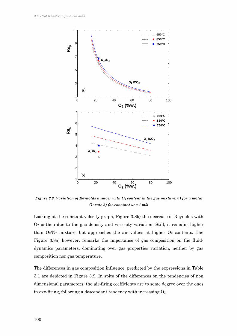
3.2. Heat transfer in fluidized beds
100
Figure 3.8. Variation of Reynolds number with O2 content in the gas mixture: a) for a molar
O2 rate b) for constant uf = 1 m/s
Looking at the constant velocity graph, Figure 3.8b) the decrease of Reynolds with
O2 is then due to the gas density and viscosity variation. Still, it remains higher
than O2/N2 mixture, but approaches the air values at higher O2 contents. The
Figure 3.8a) however, remarks the importance of gas composition on the fluid-
dynamics parameters, dominating over gas properties variation, neither by gas
composition nor gas temperature.
The differences in gas composition influence, predicted by the expressions in Table
3.1 are depicted in Figure 3.9. In spite of the differences on the tendencies of non
dimensional parameters, the air-firing coefficients are to some degree over the ones
in oxy-firing, following a descendant tendency with increasing O2.
0 20 40 60 80 1001
3
5
7
9
11
O2 (%w.)
Re p
950ºC
850ºC850ºC
750ºC750ºC
O2 /N2
O2 /CO2
0 20 40 60 80 1001
2
3
4
5
6
7
O2 (%w.)
Re p
950ºC
850ºC850ºC
750ºC750ºC
O2 /N2
O2 /CO2
a)
b)

Chapter 3. Heat transfer in CIRCE experimental oxy-fuel combustion bubbling fluidized bed
101
Figure 3.9. Effect of O2 content in the gas mixture on Nusselt number predicted by different
authors
The Figure 3.10 shows the prediction by Zabrodsky (1966), Eq. 3.2, for two gas
mixtures, O2/CO2 and O2/N2, at three temperatures. Since the gas density and gas
conductivity varied with opposite tendencies, the influence of O2 content at inlet is
almost offset. According to this, the heat transfer would be higher under oxy-firing
conditions, but the influence of O2 concentration would not be relevant. The heat
transfer coefficient decreases only 5% while increasing O2 in the mixture.
According to this expression, the effect of temperature would decrease the heat
transfer coefficient down to 8%, due to the changes on gas properties (since
radiation is not included in this expression).
Figure 3.10. Prediction of heat transfer coefficient by the Zabrodsky expression (Eq. 3.2)
20 40 60 800
2
4
6
8
10
12
14
16
O2 (%w.)
Nu
Dow & Jacob (1951) Dow & Jacob (1951)
Wen & Leva (1956)Wen & Leva (1956)
van Heerden (1951)van Heerden (1951)
Levenspiel & Walton (1954)Levenspiel & Walton (1954)
O2 /N2O2 /CO2
0 20 40 60 80 100400
410
420
430
440
450
460
470
480
O2 (%w.)
hm
ax (
W/m
2 K)
O2 / N2
950ºC950ºC850ºC850ºC750ºC750ºC
O2 / CO2

3.2. Heat transfer in fluidized beds
102
Radiation contribution from the gas phase is, in many cases, neglected in dense
bed. However, it must be carefully considered for the dilute zone of oxy-fuel
fluidized beds, since participative gas CO2 partial pressure is now higher. The
expression in Eq. 3.21 (Baukal, 2000) can be used to calculate the emissivity of a
mixture of gases:
εεεε OHCOg 22 Eq. 3.21
Being εf the emissivity of the mixture, and εCO2 and εH2O, the emissivity of the two
compounds at the operating temperature. Δε considers the overlapping of the
emission bands of H2O and CO2. Figure 3.11 shows the influence of the CO2 content
in the gas for three different cases of H2O content, considering a freeboard
temperature of 700ºC. The presence of H2O inhibits the mixture emissivity. The
value of the gas emissivity differs up to 15% for high CO2 content in the gas. At
lower gas temperature εH2O dominates over εCO2 for both air and oxy-fuel modes, at
27% O2 at inlet (Andersson and Johnsson, 2006).
Figure 3.11. Emissivity of a gas mixture of CO2 and H2O
From the variation of emissivity values in Figure 3.11 the contribution of radiation
mechanism will be treated as in air-firing case, including only the wall and
particles emissivities, and not the gas phase radiative properties.
0 10 20 30 40 50 60 70 800,32
0,33
0,34
0,35
0,36
0,37
0,38
CO2 (%)
g
15% H2 O
5% H2O
No H2O

Chapter 3. Heat transfer in CIRCE experimental oxy-fuel combustion bubbling fluidized bed
103
3.2.3 SUMMARY
Heat transfer in fluidized beds has been widely investigated along the last decades.
The movement of particles is the main responsible for the exchange of heat with
the immersed or wetted surfaces. Together with this mechanism, the gas
convection and the radiation are also involved in the overall heat transfer. In the
earlier decades, researchers looked for empirical expressions that fairly
represented the phenomena occurring during the contact of particles with the
exchange surface, through the gas layer in the proximity of the wall. In spite of
their simplicity, some predict the influences of operational parameters similarly to
the more mechanistic models. Empirical correlations, however, have been
developed usually for small rigs and their extrapolation to a different geometry and
conditions must be carefully treated. The theoretical analysis of heat transfer
during oxy-fuel in fluidized beds is assessed for the first time. The predictions from
some of the expressions forecast different values for oxy-fuel case. In most of them,
however, the value of heat transfer in oxy-fuel is slightly higher than in air-firing.
This will be quantified and analyzed in the following sections. The mechanistic
approach turns out as a suitable option for including the differences in the
fluidizing atmosphere. Particular attention should be paid to the effective
properties of the particle phase and to the residence time of particles when gas
properties change. Although the heat transfer coefficients in oxy-fuel combustion
are not expected to be far from those during air-firing, there is no study yet
pointing at this line.
From this lack of experimentation on heat transfer in oxy-fuel fluidized bed, we
now characterize the heat transfer experimentally in a pilot plant working both,
under oxy and air-firing conditions.

3.3. Experimental set-up
104
3.3 EXPERIMENTAL SET-UP
3.3.1 PREVIOUS EXPERIENCES ON OXY-FUEL FLUIDIZED BEDS
PILOT PLANTS.
In the last decade, some fluidized bed pilot plants operating under oxy-firing
conditions were erected. Details can be found in Table 1.2. In general, they
estimate the heat transfer coefficients analogously to the air-firing mode of
operation. In spite of the remarkably importance of the proper heat transfer
surfaces allocation in oxy-fuel fluidized beds, there is only one study that included
the measurement of heat transfer coefficients under oxy-fuel conditions. It was
carried out by Alstom in their 3MW Multi-Use Combustion Test Facility (Nsakala
et al., 2004). For measuring heat transfer at two different sections of the furnace,
they installed two single tube test sections in the furnace. The pipes were 2 and 11/4
inch, for assuring a high water velocity and so, low heat transfer resistance. They
concluded that there was no clear difference in the heat transfer to the test sections
between air and oxy-fuel operation. Still, they did not show any numerical results
of these measurements. Furthermore, the particular relevance that the external
heat exchanger will gain in the future oxy-fuel designs, points out the need of
measuring the heat transfer coefficient also in the dense part of the fluidized beds.
A pilot plant that were initially conceived for operating under conventional air-
firing conditions and that was retrofitted for oxy-firing should have included
additional heat removal systems or should have considered this cooling flexibility
from the initial design. It is difficult to find, in the published description of
existing oxy-fuel pilot plants, the techniques used for controlling the bed
temperature. Some of the facilities, used water cooled pipe, introduced vertically
into the fluidized bed (de Diego et al., 2012). During operation they can move the
pipe upward and downwards, controlling so the heat transfer surface and easily
regulating the temperature. In other cases, the cooling methods are less
sophisticated, and they consist of removing layers of isolating wool, for external
walls natural convection enhancement (Czakiert, 2011).
Despite there are no other studies in which attention were particularly paid to heat
transfer during oxy-fuel combustion in fluidized bed, there are important issues
Chapter 3. Heat transfer in CIRCE experimental oxy-fuel combustion bubbling fluidized bed
105
closely related to the heat removal of oxy-fuel fluidized beds and the control of bed
temperature:
‐ One of them and the most influencing for the proper future oxy-fuel large
boilers have already explained in the previous chapter, regarding the heat
transfer balance in the overall plant between AF and OF cases. The
external heat transfer in fluidized bed heat exchanger will not be fluidized
with air anymore but, most probably, with recycled flue gases. The
composition will be predominantly CO2. Probably with certain O2, H2O or N2
from air-leakages. This change in gas composition is closer to the oxy-fuel
atmosphere in a bubbling fluidized bed, as will be further explained here.
‐ Other fundamental issue regards the mechanisms of in-bed SO2 capture.
These change from usual air fluidized bed conditions. Garcia-Labiano et al.
(2011) found that higher bed temperature would be needed for obtaining
similar SO2 capture efficiencies than with air. Calcination previous sulfation
of limestone, the two-step reaction that usually occurs in conventional firing
at around 850ºC, will not take place under oxy-firing conditions. Higher CO2
partial pressure existing on oxy-fuel boilers avoid calcination of limestone at
that temperature, and thus, lower SO2 capture efficiencies. The authors
proof this in a small fluidized bed rig (de Diego et al., 2011) and
recommended higher bed temperature for optimum SO2 capture under OF.
This was confirmed at greater scale by Lupiañez et al. (2012) If higher
temperature level is needed, heat removal along the boiler requires a more
accurate design. The risk of ashes agglomeration in hot spots is then more
probable. Moreover the proper allocation of the heat transfer surfaces along
the boiler need to be carefully design for optimizing the combustor
efficiency, since higher heat recovery will be needed in the convective pass
of the boiler.
‐ Another important concern is also related to the calcination of limestone for
SO2 capture. If calcination takes place the excess of CaO arrives at the
external heat exchanger. It will meet there the fluidizing gas consisting
mostly on CO2. Below certain temperature, this CO2 would react with the
arriving CaO and the external heat exchanger could be instantaneously
defluidized. Control of temperature in this device will then be of an
essential importance, for avoiding such problem. In the literature, the 4 MW
3.3. Experimental set-up
106
pilot plant unit, owned by Metso Power, reported this kind of difficulties
(Varonen et al., 2012).
CIRCE oxy-fuel bubbling fluidized bed was initially designed based on flexibility
criteria. Different fuel ranks, from lignite to bituminous coal, and also biomass and
coal blends have been characterized under oxy-fuel combustion (Romeo et al.,
2011). A wide range of O2 percentages at inlet have also been tested. This plant has
been used by other components of the research group, for assessing the influencing
of oxy-fuel combustion on the pollutant emissions, such as NOx and SO2 (Romeo et
al., 2009b; Lupiáñez et al., 2011). Fluid-dynamics differences between AF and OF
have also been addressed (Guedea et al., 2011). Combustion performance was
analyzed and reported. The focus is addressed now towards the heat transfer
measurements and the influence of oxy-fuel conditions on it.
3.3.2 CIRCE OXY-FUEL BUBBLING FLUIDIZED BED PILOT PLANT
In 2008 erection of the oxy-fuel bubbling fluidized bed combustor was finished and
first characterization tests were run. The pilot plant was designed to burn up to 90
thermal kW under oxy-fuel conditions. Figure 3.12 represents the whole
arrangement of plant equipments. Figure 3.13 shows a picture of the facility.
The combustion takes place in a bubbling fluidized bed, 203 mm internal diameter.
Freeboard height was fixed at 1.8 m with an estimated maximum dense-bed height
of 0.7 m. A propane burner pre-heats the bed material, up to the ignition
temperature, which depends on the fuel. The induced draft fan is needed for the
preheating stage, since it facilitates combustion flue gases to be conducted along
the bed and the auxiliary equipments and so, heating up the overall facility.

Chapter 3. Heat transfer in CIRCE experimental oxy-fuel combustion bubbling fluidized bed
107
Figure 3.12. Pilot plant scheme: 1- Bubbling fluidized bed. 2-O2 supply bottles. 3-CO2 supply
bottles. 4-Propane burner pre-heater. 5- Cyclone. 6-Flue gas heat recovery exchanger. 7-Bag
filter. 8-Induce draft fan. 9-Forced or recirculation draft fan. 10-Cooling water pump. 11-
Air-Water cooler
Figure 3.13. Photo of the fluidized bed pilot plant
Regarding the fuel and fresh sorbent supply, two 0.2 m3 hoppers are located
besides the reactor. When using coal and coal mixtures, one hopper contains the
11
9
8
710
1
3
2
4
10
65

3.3. Experimental set-up
108
fuel and the other limestone. When solids with different properties are used, such
as coal and biomass, it is necessary to feed them separately, because segregation
could take place easily inside the hopper. Each hopper discharges into endless
screws controlled by variable-frequency drives and so, independent flow rates can
be fed from every hopper. Each endless screw discharges in a faster one that feeds
the combustor in the lower part, at 0.1 m over the distributor plate. While
operating the plant under air-firing conditions, a forced-draft fan (or recirculation
fan) introduces air into the boiler. When feeding oxygen with carbon dioxide
mixtures from the gas canisters, this fan is no needed but is used again when
substituting commercial CO2 by RFG. In any case, an induced-draft fan evacuates
the flue gas from the reactor. Fans nominal flow rates are 45 Nm3/h and 130
Nm3/h, respectively. O2/CO2 mixture is initially taken from 2 blocks of 12 canisters
each. The proportion of each compound in the oxidant is controlled in a gas-mixer
and the mixture is stored in small tank before it is fed. Once the operation is
stabilized, a bleed from flue gases is recycled by the recirculation-draft fan,
replacing the consumption of CO2 cylinders.
Particles present in flue gases from the fluidized bed combustor are first removed
by a fall chamber and later by a high efficiency Stairmand cyclone, designed for a
cut size of 2 µm. Sensible heat from flue gases can be used in a 9kW shell-and-tube
heat exchanger, where oxidant gas can be preheated, or by-passed depending of the
required temperature level. At the end, a fabric-filter bag is located for additional
particle retention.
For monitoring and controlling purposes, measurement instruments, valves, motor
starters and variable-frequency drivers, are connected to a PLC (Programmable
Logic Controller). Signals from thermocouples, pressure gauges, flow-meters and
control valves are connected by distributed I/O. Some automatic sequences are
programmed, to execute well-defined operating actuations. The supervision is
carried out by Supervisory Control and Data Acquisition Application (SCADA).
Initially, the bed was designed for being cooled down thanks to a cooling jacket that
covered the dense part, but the design was modified for accomplishing four
independent jackets.
The constructive division of the combustor consists of two separated zones, the
lower part, 0.8 m height, and the upper part, 1.6 m height and refractory lined. The
lower part is where most of the combustion and reactions occurs. For controlling
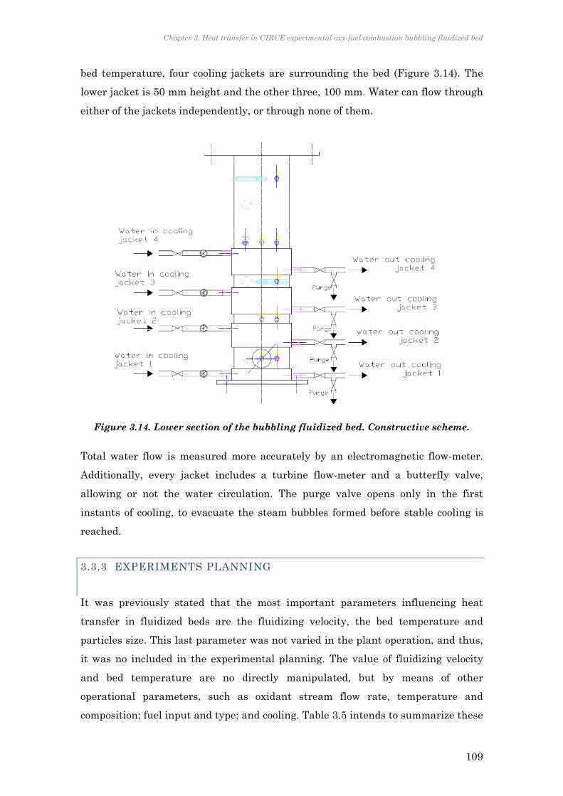
Chapter 3. Heat transfer in CIRCE experimental oxy-fuel combustion bubbling fluidized bed
109
bed temperature, four cooling jackets are surrounding the bed (Figure 3.14). The
lower jacket is 50 mm height and the other three, 100 mm. Water can flow through
either of the jackets independently, or through none of them.
Figure 3.14. Lower section of the bubbling fluidized bed. Constructive scheme.
Total water flow is measured more accurately by an electromagnetic flow-meter.
Additionally, every jacket includes a turbine flow-meter and a butterfly valve,
allowing or not the water circulation. The purge valve opens only in the first
instants of cooling, to evacuate the steam bubbles formed before stable cooling is
reached.
3.3.3 EXPERIMENTS PLANNING
It was previously stated that the most important parameters influencing heat
transfer in fluidized beds are the fluidizing velocity, the bed temperature and
particles size. This last parameter was not varied in the plant operation, and thus,
it was no included in the experimental planning. The value of fluidizing velocity
and bed temperature are no directly manipulated, but by means of other
operational parameters, such as oxidant stream flow rate, temperature and
composition; fuel input and type; and cooling. Table 3.5 intends to summarize these

3.3. Experimental set-up
110
variables limits and monitoring devices, aiming at operating inside a proper range
of values for fluidizing velocity and bed temperature.
The first column in Table 3.5 shows the parameters of the plant and inert matter
that keep constant during the tests. These are the boiler geometry, the distributor
plate arrangement, sand characteristics and its particle size distribution. The
central section of Table 3.5 indicates the variables that can be manipulated during
the plant operation. uf and T are then indirectly varied:
‐ The fluidizing velocity is determined by the stoichiometric oxygen related to
the fuel fed, the proportion of diluents: CO2, recycled flue gas or air-N2 and
the bed temperature. The temperature influences the density of gases and
thus, the velocity inside the reactor. For fitting into the desired bubbling
regime, velocities were kept between 0.8 and 1.6 m/s
‐ The bed temperature is uniform in the dense part of the bed. Oxygen
concentration affects the temperature profile. Particularly in this
installation, temperature in the freeboard will be remarkably higher under
oxy-fuel that under air-firing. Keeping temperature below 1000ºC will be
essential for avoiding agglomeration problems.
Although fuels tested in the plant ranged from anthracite to lignite and blends
with biomass, the experiments considered for the heat transfer coefficient
assessment were the ones using anthracite type of coal. The other fuels exhibited
lower heating values and so, lower thermal output during operation. As a
consequence, the heat of combustion was not enough to keep stable cooling and
heat transfer coefficients were not considered. The two types of Spanish anthracite
used in the tests are shown in Table 3.3.
The ranges of experiments planned and finally achieved are summarized in Table
3.4. The range of oxidant composition was varied in oxy-fuel mode up to 65% O2
concentration. Gas velocities were lower under oxy-fuel combustion, compared with
air-mode.

Chapter 3. Heat transfer in CIRCE experimental oxy-fuel combustion bubbling fluidized bed
111
Fuel: Anthracite 1 Anthracite 2
HHV( Kcal/kg) 5095 5350
INMEDIATE ANALYSIS (%w.)
moisture 2,05 1,00
volatile matter 10,84 7,55
fixed carbon 61,11 59,90
ashes 26,00 31,55
PROXIMATE ANALYSIS (%w.)
C 64,46 60,66
S 1,04 1,33
H 2,32 2,16
N 1,20 0,87
O 4,98 3,43
Table 3.3. Composition of fuels used in the tests
MODE O2 inlet (% v.) T bed (C) uf (m/s)
Planned Achieved Planned Achieved Planned Achieved AF N/A N/A 800-850 785-850 0,8-1 0.95
OF
25%-35% 31%-32% 800-850 - 0,8-1 - 35%-45% 36%-44% 800-850 827-855 0,8-1 0.74-0.94 45%-55% 50%-54% 800-850 - 0,8-1 - 55%-65% 57%-60% 800-850 833 0,8-1 0.86-0.98
OF-RFG 30%-35% 36-37% 800-850 796-830 0,8-1 0.84-0.85 AF N/A N/A 850-900 859-958 0,8-1 0.95
OF
25%-35% 31%-32% 850-900 877-895 0,8-1 0.84-0.98 35%-45% 36%-44% 850-900 858-964 0,8-1 0.78-0.94 45%-55% 50%-54% 850-900 889-943 0,8-1 0.82-0.98 55%-65% 57%-60% 850-900 885-918 0,8-1 0.86
OF-RFG 30%-35% 36-37% 850-900 859-887 0,8-1 0.85 AF N/A N/A 800-850 785-850 1-1,2 1.3-1.6
OF
25%-35% 31%-32% 800-850 - 1-1,2 - 35%-45% 36%-44% 800-850 827-855 1-1,2 - 45%-55% 50%-54% 800-850 - 1-1,2 - 55%-65% 57%-60% 800-850 833 1-1,2 -
OF-RFG 30%-35% 36-37% 800-850 796-830 1-1,2 1.05 AF N/A N/A 850-900 859-958 1-1,2 1.3-1.6
OF
25%-35% 31%-32% 850-900 - 1-1,2 1.02-1.23 35%-45% 36%-44% 850-900 858-964 1-1,2 1.04 45%-55% 50%-54% 850-900 889-943 1-1,2 - 55%-65% 57%-60% 850-900 885-918 1-1,2 1.05
OF-RFG 30%-35% 36-37% 850-900 859-887 1-1,2 - Table 3.4. Experiments planning matrix, planned and achieved ranges

Fixed Parameters Parameters that can be modified during operation Parameters that defined the plant
operation
Parameter Range Parameter Control device Monitoring Range Parameter Monitoring Range
Bed geometry
-207 mm
diameter
-Lower 1 m no
refractory lined
-Upper 2 m
additional
refractory lined
Gas inlet flow
rate
-Forced-draft fan with
variable-frequency
drives (AF)
-Valves (OF)
Flow-meters 30-150 m3/h Fluidization
velocity Flow-meters 0.7-1.2 m/s
Inert matter
Sand
Comburent
composition -Gas bottles mixer (OF) Gas analyzer
Air, 25%-
65%O2,
FGR
Bed
temperature
Thermo-
couples 750-980ºC
Particle size
distribution
500-800 microns
Thermal
power
Fuel endless screw with variable-frequency
drives. 30-100 kW
Distributor
plate
Flat plate with
210 orifices
Fuel Type Proximate and ultimate analysis
Coals,
biomass,
coke…
Cooling
-Valves opening to the
cooling jackets
-Aero-cooler
Water
thermocouples
Water flow-meter
5- 60 kW
Gas inlet
temperature
Proportional valve bypassing the heat
exchanger 35-180ºC
Table 3.5. Experimental operational ranges and devices

Chapter 3. Heat transfer in CIRCE experimental oxy-fuel combustion bubbling fluidized bed
113
3.4 HEAT TRANSFER COEFFICIENTS MEASUREMENT
3.4.1 MEASURING PROCESS
Heat transfer coefficients are measured by an indirect way. When cooling is
required for keeping a proper bed temperature, one of the cooling jackets valve is
opened, at inlet, allowing water to pass through it. In the first instant of water
crossing the jacket, the purge valve is opened. Water is around 40ºC when it enters
the jacket, and the bed wall is near bed temperature, at more than 850ºC. Thus,
during cooling start a great overpressure takes place, because of steam bubbles
generation. Opening the purge valve releases this initial steam, protecting also the
welding of the jackets. When water is not vaporized anymore, the purge valve is
closed and the valve at outlet is opened, to close the water circuit. Heat transfer
coefficient is measured at this instant.
Water mass-flow measurements and water temperature are averaged for every
cooling period to calculate the energy removed by the water is approximated with
Eq. 3.22:
INwater;OUTwater;cooling TTcmQ Eq. 3.22
Being m the water mass flow, c the average water thermal capacity and Twater;OUT
and Twater;IN temperatures at outlet and inlet of the cooling jacket respectively. This
expression assumes the approximation of considering the water calorific value, c,
constant at the water average temperature.
The energy transferred to the cooling jackets is analogous to the Newton Cooling
Law, calculated by means of the global heat transfer coefficient UA, yielding:
ΔTUAQcooling Eq. 3.23
ΔT is the logarithmic temperature difference evaluated as:
OUTwater;bed
INwater;bed
INwater;OUTwater;
T-T
T-Tln
T-TΔTln
Eq. 3.24
3.4 Heat transfer coefficients measurement
114
Bed temperature is measured at different heights in the bed. Particularly the
temperature measured at the lowest position is located at 99 mm from the
distributor. Then, bed temperature of the first jacket is approximated to the
average between the oxidant stream temperature and the value from the first
thermocouple.
Neglecting the conduction through the bed wall, UA involves two main
contributions, the water convection coefficient, hwater, and the fluidized bed
coefficient, hbed:
bedbedwaterwater Ah
1
Ah
1
UA
1
Eq. 3.25
Water circulates through the jacket at high velocity, since the jacket is only 6 mm
width. Water convection heat transfer coefficient is estimated using the formula by
Gnielinsky, recommended by Mills (1995), for calculating heat transfer coefficient
in the water side. The water heat transfer coefficient reaches values around 2500
W/m2K. This is around an order of magnitude higher than the heat transfer
coefficient in fluidized beds and, it can be neglected from Eq. 3.25.
Following criteria have been established for selecting an appropriate time-
framework of measurements:
‐ At least 1 minute of stable operation on water parameters: mass flow rate
and temperature at outlet and inlet (avoiding bubbling phase)
‐ During this time, fed fuel must be also constant
‐ During this time, fan drivers frequency is not varied.
‐ Registered emissions delays at least 3 minutes after any change inside the
combustor. With this premise, 1 minute of stability in emissions
measurements is also considered after the moment of stability in the water
parameters.
‐ Values for calculations are averaging over the stability range selected
‐ The number of values increases when the time framework is longer, and
this will allow reducing uncertainty, as it will be later explained.
A usual cooling curve is shown in the Figure 3.15. Here they are represented the
water inlet and outlet temperature, the water flow rate and, in the secondary axle,
the bed temperature. The frame remarks the time of operation at which values of
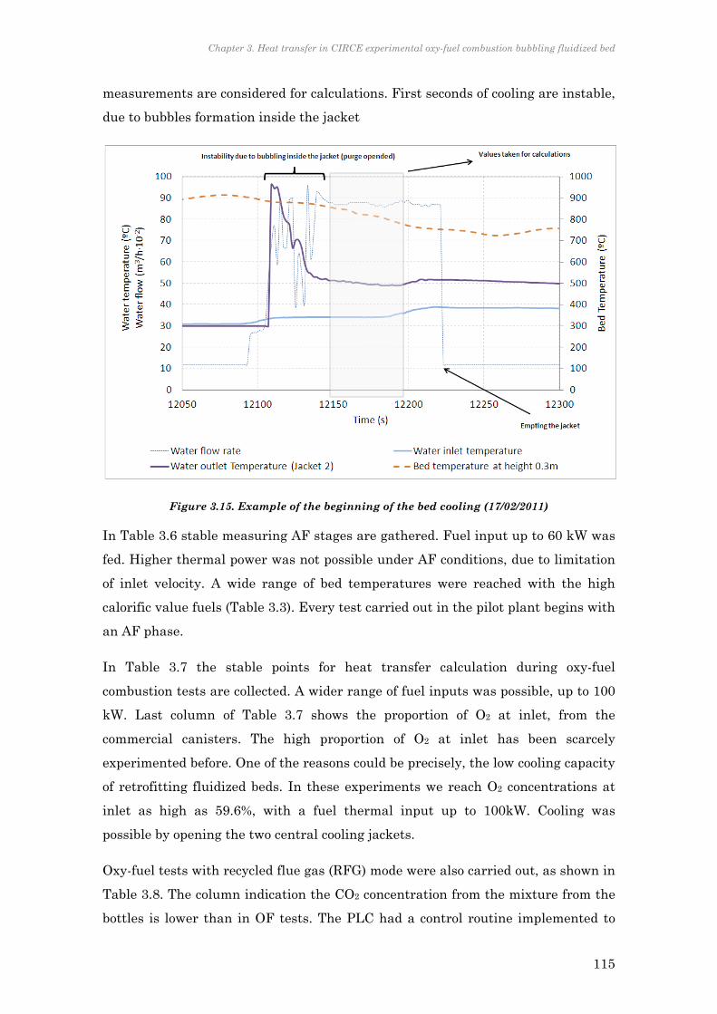
Chapter 3. Heat transfer in CIRCE experimental oxy-fuel combustion bubbling fluidized bed
115
measurements are considered for calculations. First seconds of cooling are instable,
due to bubbles formation inside the jacket
Figure 3.15. Example of the beginning of the bed cooling (17/02/2011)
In Table 3.6 stable measuring AF stages are gathered. Fuel input up to 60 kW was
fed. Higher thermal power was not possible under AF conditions, due to limitation
of inlet velocity. A wide range of bed temperatures were reached with the high
calorific value fuels (Table 3.3). Every test carried out in the pilot plant begins with
an AF phase.
In Table 3.7 the stable points for heat transfer calculation during oxy-fuel
combustion tests are collected. A wider range of fuel inputs was possible, up to 100
kW. Last column of Table 3.7 shows the proportion of O2 at inlet, from the
commercial canisters. The high proportion of O2 at inlet has been scarcely
experimented before. One of the reasons could be precisely, the low cooling capacity
of retrofitting fluidized beds. In these experiments we reach O2 concentrations at
inlet as high as 59.6%, with a fuel thermal input up to 100kW. Cooling was
possible by opening the two central cooling jackets.
Oxy-fuel tests with recycled flue gas (RFG) mode were also carried out, as shown in
Table 3.8. The column indication the CO2 concentration from the mixture from the
bottles is lower than in OF tests. The PLC had a control routine implemented to
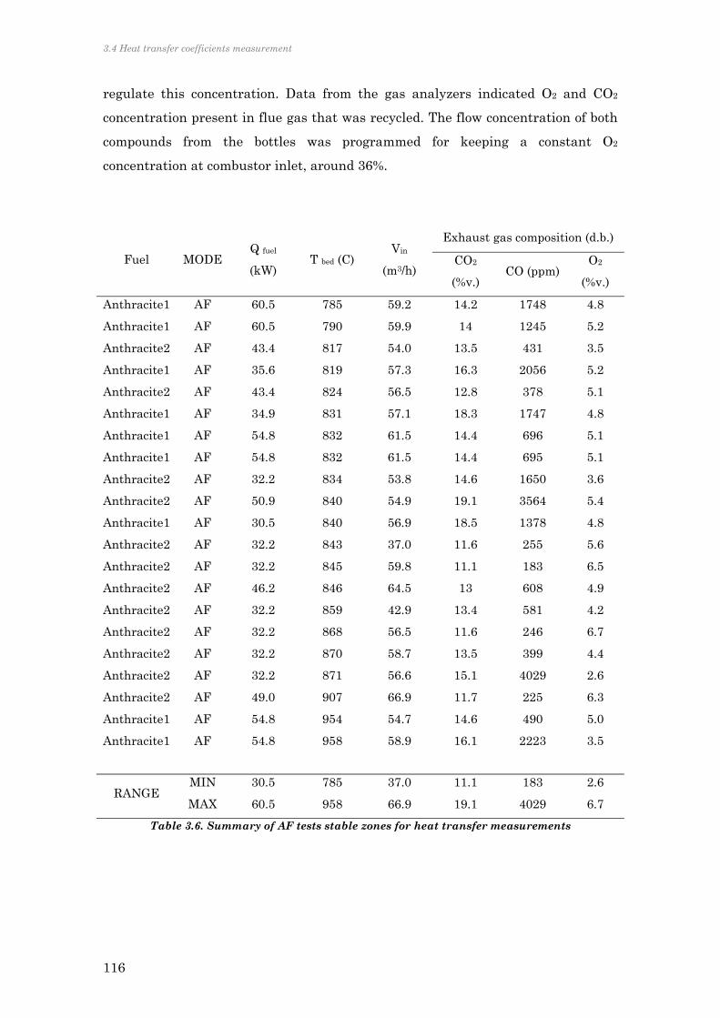
3.4 Heat transfer coefficients measurement
116
regulate this concentration. Data from the gas analyzers indicated O2 and CO2
concentration present in flue gas that was recycled. The flow concentration of both
compounds from the bottles was programmed for keeping a constant O2
concentration at combustor inlet, around 36%.
Fuel MODE Q fuel
(kW) T bed (C)
Vin
(m3/h)
Exhaust gas composition (d.b.)
CO2
(%v.) CO (ppm)
O2
(%v.)
Anthracite1 AF 60.5 785 59.2 14.2 1748 4.8
Anthracite1 AF 60.5 790 59.9 14 1245 5.2
Anthracite2 AF 43.4 817 54.0 13.5 431 3.5
Anthracite1 AF 35.6 819 57.3 16.3 2056 5.2
Anthracite2 AF 43.4 824 56.5 12.8 378 5.1
Anthracite1 AF 34.9 831 57.1 18.3 1747 4.8
Anthracite1 AF 54.8 832 61.5 14.4 696 5.1
Anthracite1 AF 54.8 832 61.5 14.4 695 5.1
Anthracite2 AF 32.2 834 53.8 14.6 1650 3.6
Anthracite2 AF 50.9 840 54.9 19.1 3564 5.4
Anthracite1 AF 30.5 840 56.9 18.5 1378 4.8
Anthracite2 AF 32.2 843 37.0 11.6 255 5.6
Anthracite2 AF 32.2 845 59.8 11.1 183 6.5
Anthracite2 AF 46.2 846 64.5 13 608 4.9
Anthracite2 AF 32.2 859 42.9 13.4 581 4.2
Anthracite2 AF 32.2 868 56.5 11.6 246 6.7
Anthracite2 AF 32.2 870 58.7 13.5 399 4.4
Anthracite2 AF 32.2 871 56.6 15.1 4029 2.6
Anthracite2 AF 49.0 907 66.9 11.7 225 6.3
Anthracite1 AF 54.8 954 54.7 14.6 490 5.0
Anthracite1 AF 54.8 958 58.9 16.1 2223 3.5
RANGE MIN 30.5 785 37.0 11.1 183 2.6
MAX 60.5 958 66.9 19.1 4029 6.7
Table 3.6. Summary of AF tests stable zones for heat transfer measurements

Chapter 3. Heat transfer in CIRCE experimental oxy-fuel combustion bubbling fluidized bed
117
Fuel MODE Q fuel
(kW)
T bed
(C)
Vin
(m3/h)
Exhaust gas composition
(d.b.) O2 inlet
(%v.) CO2
(%v.)
CO
(ppm)
O2
(%v.)
Anthracite1 OF 30.5 888 50.2 72.8 246 17.4 30.9
Anthracite1 OF 30.5 889 50.1 84.6 348 7.7 31.1
Anthracite1 OF 30.7 894 52.1 87.7 2635 4.7 31.2
Anthracite2 OF 71.4 877 43.7 79.7 166 8.9 31.2
Anthracite1 OF 50.3 896 62.3 90.8 1830 4.6 31.3
Anthracite1 OF 66.1 884 57.6 90.2 3527 3.3 31.4
Anthracite2 OF 54.6 882 45.2 80.2 241 9.1 32.0
Anthracite2 OF 32.5 847 39.0 79.9 2016 3.5 36.3
Anthracite2 OF 50.3 861 48.5 78.6 288 5.5 37.0
Anthracite2 OF 51.8 831 48.5 76.7 223 6.9 37.2
Anthracite2 OF 49.0 858 48.5 76.8 224 6.8 37.3
Anthracite2 OF 64.4 827 47.7 76.5 224 7.2 37.3
Anthracite2 OF 32.2 964 42.6 79.2 5120 1.9 40.8
Anthracite1 OF 50.9 891 51.4 81.0 1310 7.2 41.2
Anthracite1 OF 50.9 893 44.2 85.0 2756 6.2 41.3
Anthracite2 OF 32.2 944 37.1 79.2 5120 2.5 41.8
Anthracite2 OF 32.6 898 39.8 78.0 306 8.2 43.0
Anthracite2 OF 54.6 884 41.6 76.8 250 9.3 43.9
Anthracite2 OF 68.3 902 44.2 80.2 380 9.2 49.9
Anthracite2 OF 72.3 943 44.8 79.6 200 7.0 50.4
Anthracite2 OF 74.4 895 45.3 79.7 375 8.5 50.5
Anthracite2 OF 77.0 889 43.4 69.9 300 13.4 50.7
Anthracite2 OF 77.0 918 38.4 67.1 319 15.8 50.9
Anthracite2 OF 78.0 894 43.6 72.4 283 13.1 53.5
Anthracite2 OF 77.0 918 48.3 77.9 227 6.2 57.5
Anthracite2 OF 99.4 833 48.4 65.5 434 18.0 57.8
Anthracite2 OF 99.4 885 40.4 75.6 5045 6.9 59.6
RANGE MIN 30.5 827 37.1 65.5 166 1.9 30.9
MAX 99.4 964 62.3 90.8 5120 18.6 59.6
Table 3.7. Summary of OF tests stable zones for heat transfer measurements

3.4 Heat transfer coefficients measurement
118
Fuel MODE Q fuel
(kW)
T bed
(C)
Vin
(m3/h)
Exhaust gas composition
(d.b.) CO2
bottles
(%v.) CO2
(%v.)
CO
(ppm) O2 (%v.)
Anthracite2 OF+RFG 65.8 887 49.2 55.6 1332 5.7 34.7
Anthracite2 OF+RFG 65.8 864 49.3 49.2 284 7.1 30.3
Anthracite2 OF+RFG 77.0 796 46.8 48.9 218 9.0 30.4
Anthracite2 OF+RFG 77.0 830 45.6 47.9 267 9.8 30.5
RANGE MIN 50.7 796.5 26.9 41.1 218.2 5.7 30.3
MAX 77.0 886.6 49.3 55.6 2977.3 23.8 44.4
Table 3.8. Summary of OF+RFG tests stable zones for heat transfer measurements
3.4.2 HEAT TRANSFER RESULTS
The results of the heat transfer coefficient estimations for the bed to the wall in
every mode are then calculated and represented in Figure 3.16.
Figure 3.16. Fluidized bed heat transfer coefficients measured in each jacket
0
100
200
300
400
500
600
700
h (
W/m
2K
)
Air-firing Oxy-firing Oxy-firing with RFG
Jacket 1 Jacket 2 Jacket 3 Jacket 4
Chapter 3. Heat transfer in CIRCE experimental oxy-fuel combustion bubbling fluidized bed
119
The most important conclusion drawn from Figure 3.16 is that values estimated for
AF, OF and OF+RFG modes of operation are enclosed within similar ranges,
within 200 to 600 W/m2K. These results demonstrate and agree with the
fundamental mechanism of heat transfer in the bubbling beds, based on the
movement of particles and their contacts with the wall, rather than on the gas
composition.
In the fourth jacket, the values are the lowest. This is because it is located at the
limit height of the dense bed, coinciding with the exploding bubbles zone. Bed
density here is lower and so it is the influence of particle convection heat transfer.
The first jacket exhibits the widest dispersion of coefficients. The geometry of this
jacket is slightly different from the others. It is half height and it is welded to the
lower flange. At first sight this disposition can be act as an extended surface for
heat transfer and could influence the heat transfer evaluation. After a transient
heat transfer evaluation in this zone the influence of the flange was not relevant
for the heat transfer coefficients results. The reason of the lower values in first
jacket resides then on the temperature of this zone, where cool oxidant enters the
combustor, rapidly reacts with the fuel present and increases the temperature,
creating a temperature peak in the zone near the distributor. So, the temperature
of the bed at the first jacket location, below the first thermocouple, is lower than in
the rest of the bed in many cases.
In all tests, the bed height is higher than the third jacket, so the second and third
jacket heat transfer coefficients dwell within a narrower range of values. The three
modes of operation show closer values. The discussion will lie in the factors
influencing heat transfer and the role of oxy-fuel atmosphere on the influences of
the heat transfer coefficients, in section 3.3.4.
The following section explores the uncertainties of these measurements, as criteria
to accept or reject any of the measurements.

3.4 Heat transfer coefficients measurement
120
3.4.3 UNCERTANITY ANALYSIS
In order to complete the previous results, we must evaluate the uncertainties, due
to deviations in the sensors measurements and averaging process, from which they
are calculated.
h must be expressed as a function of water volumetric flow and inlet and outlet
temperature, bed temperature and the properties of water, ρ and c, at the average
temperature:
ΔTlnA
TTc3600Vρ
hcooling
INwater;OUTwater;water
Eq. 3.26
Uncertainties associated with heat transfer coefficients are calculated by
propagation of uncertainties principle Eq. 3.27 (Coleman and Steele, 1999):
2
OUTwater;
T
2
OUTwater;
OUTwater;
2
INwater;
T
2
INwater;
INwater;2
2h
T
U
T
h
h
T
T
U
T
h
h
T
h
U OUTwater;INwater;
2
A
22
V
22
bed
T
2
bed
bed
A
U
A
h
h
A
V
U
V
h
h
V
T
U
T
h
h
Tned
.. Eq. 3.27
Where Uh, UTwaterIN, UTwater,OUT, UTbed and UTA are the uncertainties related to the
corresponding variables, respectively: heat transfer coefficient h, inlet and outlet
TwaterIN and TwaterOUT, bed temperature Tbed and cross sectional area for the water
flow, A. This area is considered a constant value during each experiment.
The PLC registers the measurements every two seconds. Each instant, h is
calculated and averaged within the stability period. Every instantaneous measure
of h has an uncertainty associated with the measurements device and calculated by
Eq. 3.27.
The systematic uncertainty of the thermocouples type K was calculated from the
standard limit of errors, 0.75%, using Eq. 3.28.
3
limitU
2
T Eq. 3.28
The water flow measurement given by the turbine flow-meters was calibrated with
the electromagnetic flow-meter, since this is a much more accurate device. The

Chapter 3. Heat transfer in CIRCE experimental oxy-fuel combustion bubbling fluidized bed
121
systematic error includes then a term for the absolute uncertainty of both,
electromagnetic and turbine devices and the influence of temperature. The
absolute uncertainty of volume flow yields:
3
ΔVUUKU
2etemperatur2
ncalibratio2sampleV Eq. 3.29
Since the instantaneous value of h is averaged during the measuring period, the
variance and the number of samples must be included and the absolute uncertainty
of h yields:
m
m2ousinstantaneh n
SUKU
2
Eq. 3.30
Where, Sm2 is the variance of the measurements of h along the period of time
considered. The constant K is usually equal to 2, assuming an enough number of
data for the calculation. Instantaneous and absolute uncertainties are summarized
in Table 3.9, averaging the uncertainties obtained for each value of h measured:
Instantaneous uncertainty Sample period uncertainty
Jacket 1 2 3 4 1 2 3 4
max Uh 5.8% 2.6% 2.9% 3.8% 10.8% 1.6% 1.5% 8.8%
min Uh 28.4% 8.1% 11.6% 7.2% 34.3% 25.8% 30.3% 10.1%
average Uh
11.6% 5.2% 5.0% 5.1% 18.8% 9.3% 10.8% 9.5%
Table 3.9. Instantaneous and averaging relative uncertainty for heat transfer determination
The results of the instantaneous uncertainties assigned the most important source
of errors to the water thermocouples, since the possible range of measurement of
this device is much wider than the values of water temperature. The jackets 2, 3
and 4, presented uncertainties around 5% in the measurement of h, whereas the
jacket 1 showed higher values, up to 12% averaged.
In the following analysis we discard the values obtained in the first jacket, since
they involve double uncertainty ranges than the other three. We must also remove
the fourth jacket measurements, because, as previously explained, the bed limit is
below the jacket and thus the conditions are not comparable with the other jackets.
Finally, the measurements of heat transfer during the OF+RFG mode will not be
considered, since they are too few to be representative.
3.5 Discussion on the results of heat transfer in oxy-fuel BFB
122
3.5 DISCUSSION ON THE RESULTS OF THE HEAT
TRANSFER IN OXY-FUEL BFB
Along the current section, the results obtained of heat transfer during air and oxy –
combustion tests are analyzed under the two perspectives revised in section 3.2.
First, non-dimensionalized heat transfer values are compared with the
conventional non-dimensional numbers involved in the majority of empirical
approached for particle convection. Additionally, the expression by Molerus (Eq.
3.3) will also be explored and it will better estimate the influence of Reynolds
number. The measurements will be then contrasted with the semi-empirical
mechanistic approaches for heat transfer calculation. Here it is proposed the
expression that better fits the experimental values in oxy-fuel combustion. This
approach aims at being extrapolated to different facilities of similar characteristics,
such as external heat exchangers attached to circulating fluidized beds.
3.5.1 EMPIRICAL APPROACH ANALYSIS
The theoretical distribution of non-dimensional numbers in oxy-fuel fluidized bed
combustion was reviewed at the beginning of this chapter. Now, the experimental
results are shown in terms of these set of parameters, in order to forecast the
experimental heat transfer obtained during the operation.
Figure 3.17 shows the non-dimensional numbers calculated from the experimental
conditions, and represented as a function of the O2 content at inlet of the reactor.
The Archimedes number is slightly higher in OF than AF. These values get closer
for higher O2 concentrations. The bed temperature in AF is in general lower than
in OF, and this makes the values of Archimedes in OF approach those in AF.
Analogously, Reynolds in OF is close or even lower than in AF. Apart from the bed
temperature influence, as in Archimedes case, fluidizing velocities in AF were
higher than in OF in the majority of cases, approaching so the values of both
modes. Finally, Prandtl number follows the theoretical curve represented in Figure
3.7, where the temperature influence affects the AF values, but not OF.

Chapter 3. Heat transfer in CIRCE experimental oxy-fuel combustion bubbling fluidized bed
123
Figure 3.17. Influence of O2 content on non-dimensional parameters
Although fully empirical expressions cannot assure and accurate estimation of heat
transfer coefficient values for conditions different from those used for their
development, they can help to anticipate influences of different non-dimensional

3.5 Discussion on the results of heat transfer in oxy-fuel BFB
124
numbers on Nusselt numbers, representing the dissimilar conditions of air and
oxy-firing modes. Similarly to the theoretical analysis carried out at the beginning
of this chapter, the influence of non-dimensional numbers is here evaluated with
the experimental results.
In Figure 3.18 the experimental Nusselt number is compared with the Prandtl,
Reynolds, Archimedes, heat thermal capacity ratio, thermal conductivity ratio and
bulk-gas density ratio.
Figure 3.18.Influence of non-dimensional parameters on Nusselt number

Chapter 3. Heat transfer in CIRCE experimental oxy-fuel combustion bubbling fluidized bed
125
Prandtl number is slightly higher in OF than AF, around 2%, so the influence on
Nusselt number is not evident. Values of Archimedes numbers are overlapped
between AF and OF and no tendencies are distinguished on the Nusselt number.
Conductivity ratios seem not to affect the heat transfer at first sight, in spite of
being a predominant factor on heat transfer. Density ratios influence is not obvious
here, mainly due to the narrow range of voids fraction for keeping the bubbling
regime of fluidization. Reynolds number and the ratio of thermal heat capacities
turn out as the two factors affecting heat transfer perceptively. Both show higher
values in air-firing and increasing tendency with O2 at inlet. This agrees with the
known influences explored in the literature widely.
During air-firing tests, gas velocities were mostly higher than in oxy-firing. Gas
velocities, together with particle diameter and bulk density, are the three factors
dominating particle convection mechanism. The particle diameter is not changing
during the tests, and the bulk density is strongly influenced by the fluidizing
velocity, but also by the gas conditions of gas and viscosity. Aiming at isolating the
effect of fluidizing velocity on the influence of non-dimensional parameters on heat
transfer, we now look now at two tests of air and oxy-firing with similar fluidizing
velocity. In Figure 3.19 we represent Nusselt numbers from the tests of close
fluidizing velocity in air and oxy-firing, corresponding to 1.2 m/s and 0.95-1 m/s,
respectively. They coincide with the maximum velocity range during oxy-firing and
the minimum in air-firing. O2 concentration at inlet ranged from 50% to 57%, the
maximum values tested. Temperature varied between 832ºC and 918ºC. In the air-
firing case, temperature was 887ºC, also among the highest values reached.
By isolating the gas velocity effect, the variation of Reynolds number with gas
properties is considerably lower. The ratio of thermal capacities involves both,
variation of temperature and also, changes on gas composition. The value of
Nusselt number in the air-firing case is now more similar to the ones during oxy-
firing. None of the non-dimensional numbers in Figure 3.19 evidence any clear
tendency of Nusselt number.

3.5 Discussion on the results of heat transfer in oxy-fuel BFB
126
Figure 3.19. Influence of non-dimensional parameters on Nusselt number for similar
fluidizing velocities
In Figure 3.20 the values of similar temperature, ranging from 823ºC to 884ºC are
represented. In these graphs, the influence of the parameters on Nusselt number
can be better distinguished. Lower Reynolds numbers in OF diminishes Nusselt
with respect to AF cases. Gas conductivity for similar temperatures also displays
an effect on heat transfer, keeping lower in OF tests. In general, Nusselt numbers
in the OF tests are below the ones obtained during AF.

Chapter 3. Heat transfer in CIRCE experimental oxy-fuel combustion bubbling fluidized bed
127
Figure 3.20. Influence of non-dimensional parameters on Nusselt number for similar bed
temperature
Reynolds influence appears then as the distinguishing factor between air and oxy-
firing due to differences on gas velocity. For this reason, the Molerus model
(Molerus et al., 1995b), turns out more appropriate for evaluating the experimental
results and it is going to be following explored.
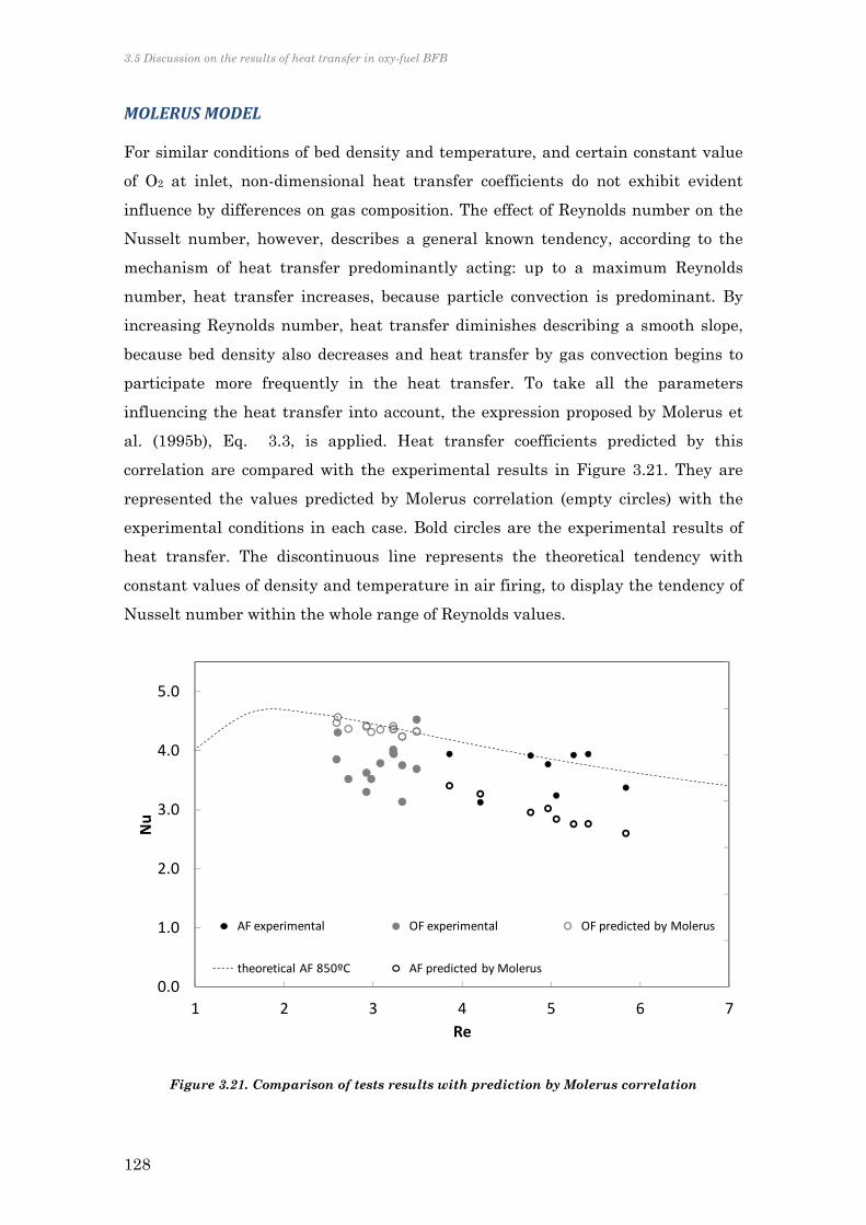
3.5 Discussion on the results of heat transfer in oxy-fuel BFB
128
MOLERUS MODEL
For similar conditions of bed density and temperature, and certain constant value
of O2 at inlet, non-dimensional heat transfer coefficients do not exhibit evident
influence by differences on gas composition. The effect of Reynolds number on the
Nusselt number, however, describes a general known tendency, according to the
mechanism of heat transfer predominantly acting: up to a maximum Reynolds
number, heat transfer increases, because particle convection is predominant. By
increasing Reynolds number, heat transfer diminishes describing a smooth slope,
because bed density also decreases and heat transfer by gas convection begins to
participate more frequently in the heat transfer. To take all the parameters
influencing the heat transfer into account, the expression proposed by Molerus et
al. (1995b), Eq. 3.3, is applied. Heat transfer coefficients predicted by this
correlation are compared with the experimental results in Figure 3.21. They are
represented the values predicted by Molerus correlation (empty circles) with the
experimental conditions in each case. Bold circles are the experimental results of
heat transfer. The discontinuous line represents the theoretical tendency with
constant values of density and temperature in air firing, to display the tendency of
Nusselt number within the whole range of Reynolds values.
Figure 3.21. Comparison of tests results with prediction by Molerus correlation
0.0
1.0
2.0
3.0
4.0
5.0
1 2 3 4 5 6 7
Nu
Re
AF experimental OF experimental OF predicted by Molerus
theoretical AF 850ºC AF predicted by Molerus

Chapter 3. Heat transfer in CIRCE experimental oxy-fuel combustion bubbling fluidized bed
129
The higher gas velocities in air-firing operation, locates the operational window
further from the optimal heat transfer coefficient. Still, since this maximum is
different in both modes, within this range of operation, the values of heat transfer
remains close in air and oxy-firing.
Molerus et al. correlation fairly fits the tendency of heat transfer during oxy-fuel
combustion, although this expression slightly over-predicts the experimental
results, particularly far from the optimum heat transfer value. The correlation
derived from cold tests at a wide range of velocities and particle diameters,
although they also validated their results with data from the literature. The fitting
curve with high temperature measurements, did not fit as good as the cold tests.
This influence of gas temperature on gas properties would lead to the over-
prediction observed in Figure 3.21.
Empirical correlations exhibit an obvious simplicity for the estimation of heat
transfer, but semi-empirical models based on mechanistic approach have more
predictive power and their use is extended in the last decades. Both modeling
strategies must account for the contribution of heat transfer by radiation.
3.5.2 CONTRIBUTION OF RADIATION HEAT TRANSFER
For dense fluidized beds, like the case of the bubbling regime, the contribution of
radiation to the overall heat transfer is rather smaller than in more diluted zones.
This is because it is the first layer of particles the one that contributes to radiation.
This layer hinders the radiation stemming from the particles in the core of the bed.
The contribution of radiation to the overall heat transfer is calculated with Eq.
2.25, including the concept of “radiation efficiency” used in the previous chapter
and proposed by Breitzholz and Leckner (1997). The results are shown in Figure
3.22.
According to Botterill (1989), apparent emissivities are around 0.43, when wall
temperature was 300ºC, and up to 0.78 when wall temperature was 850ºC. They
include these terms to account for the lower temperature of the particles adjacent
to the wall and so, the reduced contribution to radiation. Values obtained using
this methodology is slightly over the ones predicted by Figure 3.22. The
percentages obtained in Figure 3.22 agree with those collected by Glicksman and
Decker (1982).
3.5 Discussion on the results of heat transfer in oxy-fuel BFB
130
Figure 3.22. Estimation of the variation of radiant heat transfer coefficient with bed
temperature
The heat transfer contribution by radiation during oxy-fuel tests reached similar
values to those estimated for air-firing tests. This would not be the case in a more
diluted zone of the combustor. The higher CO2 partial pressure in flue gases
increases the emissivity of the flue gas mixture and the contribution of radiation
from gaseous phase will be higher. This was not evaluated here, since no heat
transfer surfaces were located in the higher part of the combustor and gas
radiation contribution could be neglected.
3.5.3 MECHANISTIC APPROACH AND PROPOSAL OF
MODIFICATION FOR OXY-FUEL CONDITIONS
The trend in the modeling of heat transfer goes towards using more realistic
approaches, as explained in section 3.1. Still, empirical expressions must be
included for those terms difficult to measure, like the effective conductivity and the
residence time of particles at the wall, with the aim of effectively simplify the
prediction of heat transfer coefficients. Heat transfer will be then the addition of
the radiation mechanism contribution, hr, and the heat transfer by particle
convection, during the contact time of the packets with the surface, accounting for
the film resistance of the gaseous layer at the heat transfer surface:

Chapter 3. Heat transfer in CIRCE experimental oxy-fuel combustion bubbling fluidized bed
131
filmpacket
br
hh
hh11
1)1(
Eq. 3.31
Where hpacket is the transient conduction of heat from the particles packet to the
surface, by integrating Eq. 3.4. If considering all packets contacting the surface for
the same length of time, τ, this term becomes (Kunii and Levenspiel, 1991):
21
,113.1
spmfseff
packet
ckh Eq. 3.32
The gas resistance, hfilm, proposed by Baskakov (1964) accounts, time-
independently, for the variation of the gas layer properties. The packet renewal
term predicted excessively high heat transfer coefficients for short particle
residence times (Botterill, 1989) and this induced to include an additional series
thermal resistance. This term was much influenced by gas thermal conductivity
and particle diameter and it can be defined as:
p
gfilm d
kMh Eq. 3.33
The term of film resistance offers the possibility of straightforward taking into
consideration the change on gas composition in oxy-fuel combustion and its
influence on the heat transfer coefficient.
The reviewed expression by Zhargami et al. (2007) for residence time prediction,
together with the model for the effective thermal conductivity explained by Xavier
and Davidson (1985), Eq. 3.9, is applied to deduced the best value of the empirical
variable M, in order to properly correlate the experimental values obtained on heat
transfer.
The maximum and average deviations of Eq. 3.31 with the experimental results
are represented in Figure 3.23, for different values of M. The minimization of these
functions indicates that, the best value of M for oxy-firing case, to optimize the
maximum deviation, is 5.47, whereas for air-firing, this parameter reaches 10.64.
To optimize the average deviation between predicted and experimental values, the
parameter M increases. The fitting process suggests 6.51, as appropriate value to
reach average deviations of 8.6% in oxy-fuel tests. For air-firing case, this value
becomes 11.33, achieving average deviations of 10.2%.

3.5 Discussion on the results of heat transfer in oxy-fuel BFB
132
Figure 3.23. Maximum and average deviation of predicted values for different values of M
The expression for estimating the heat transfer coefficient by using the mechanistic
approach yields:
1/2
1
cc
cb
bb
bepp,pmfpgpg
k
k0.057log0.757logε0.28
g
sg
packet
uδ
d6.52δ
uδ
d0.7δcε1ρudc0.1ρ
k
kk...
h
g
s
...
keff τ
Eq. 3.34
p
gfilm d
kMh with M=6.51 for oxy-firing and M=11.33 for air-firing Eq. 3.33
Figure 3.24 represents the comparison of the calculated heat transfer coefficients
and the experimental values obtained during air-firing and oxy-firing tests. In
Figure 3.24 a) the heat transfer coefficients obtained and predicted for the particle
convection contribution is represented. Values in both mode of operation are
satisfactorily predicted.
Figure 3.24b) illustrates the Nusselt number calculated for the global heat transfer
coefficient, i.e., taking the radiation term into consideration. The higher values
obtained in air-firing are due to the higher value of gas conductivity in the oxy-fuel
cases.
There are not public results on heat transfer coefficients in oxy-fuel dense fluidized
beds. Thus, validation is not possible for a different plant arrangement, as it would
be desirable.
0%
10%
20%
30%
40%
50%
60%
70%
4 6 8 10 12 14
Maxim
um deviation
M
OF
AF
0%
10%
20%
30%
40%
50%
60%
70%
4 6 8 10 12 14
Average
deviation
M
AF
OF

Chapter 3. Heat transfer in CIRCE experimental oxy-fuel combustion bubbling fluidized bed
133
Since the basis of the Eq. 3.31 to Eq. 3.36 lies on the mechanistic model, already
used in a wide range of facilities, the proposed expression for heat transfer under
oxy-firing conditions would be capable to estimate the heat transfer coefficients
from bubbling fluidized bed to surface, for an atmosphere different from air, as in
the case of external heat exchangers of large circulating fluidized beds
Figure 3.24. Validation of calculated heat transfer coefficients
.
0
200
400
600
0 200 400 600
h model
h experimental
AF
OF
+25%
‐25%
0
1
2
3
4
5
0 1 2 3 4 5
Nu model
Nu experimental
AF
OF
+25%
‐25%
a)
b)
3.6. Conclusions
134
3.6 CONCLUSIONS
For the first time the heat transfer coefficients during oxy-fuel combustion in a
bubbling fluidized bed have been quantified and presented. Measurements were
carried out during the combustion experiments in the CIRCE BFB, operated under
conventional air-firing conditions, oxy-fuel with O2/CO2 from commercial canisters
and O2 with RFG. Due to the plant flexibility, operation conditions varied along a
wide range of O2 concentrations at inlet and bed temperatures. Heat transfer data
were collected during the cooling stages in the plant operation.
The extended literature on heat transfer in fluidized bed traditionally approaches
the prediction of the coefficients by two ways, fully empirically by experimental
correlations, or by semi-empirical mechanistic models. The available studies on
heat transfer in bubbling fluidized beds are found in the earliest studies on this
issue, particularly to vertical walls instead of tubes bundles. In the last decades,
further effort was devoted to heat transfer in the transport zone of circulating
fluidized beds, since the majority of steam generation heat transfer tubes are
located in this zone. However, the relevance of heat transfer in bubbling beds, with
atmospheres different from the conventional air-firing ones, turns now up again as
a key issue, due to the importance of external heat exchanger on future large CFB
oxy-fuel boilers.
The values of heat transfer during air-firing and oxy-firing operation allowed here
the assessment of the particular key factors that differentiate both operational
modes.
The non-dimensional analysis, indicated that, the change in Reynolds, Prandtl and
Archimedes number, caused by the variation of gas composition, is offset by the
differences on fluidized gas velocity. Additionally, bed temperature in oxy-fuel
cases were over that in air combustion, bringing closer the Reynolds and
Archimedes numbers in both, AF and OF. In most of the tests, fluidizing velocity
was lower in oxy-firing tests than in air-firing. According to Molerus correlation,
this translates into higher heat transfer coefficients, because the operational points
locate closer to the optimum Reynolds number for heat transfer. However, this
correlation over-predicted the values obtained during oxy-fuel combustion.

Chapter 3. Heat transfer in CIRCE experimental oxy-fuel combustion bubbling fluidized bed
135
The mechanistic approach is recommended to more adequately predict heat
transfer coefficients. It was propose the appropriate expression to estimate the
residence time and effective thermal conductivity, among those available in the
literature. The empirical variable included in the film resistance expression shows
different values for air and oxy-firing. The results of heat transfer coefficients in
oxy-firing mode were then satisfactorily predicted.

136

137
CHAPTER 4
THE INFLUENCE OF SOLIDS
RECIRCULATION ON HEAT TRANSFER IN
AN EXTERNAL HEAT EXCHANGER
4.1 INTRODUCTION
In oxy-fuel CFB, the external heat exchanger (EHE) presents two particularities,
with respect to the conventional air-firing CFB. The one related to the change on
gas composition has been previously addressed. With the experiments in the oxy-
fuel bubbling fluidized beds, we could propose the adequate semi-empirical
expressions to predict the heat transfer coefficients. This allows including the
influence of gas composition on both, the effective thermal conductivity and the
residence time of particles, so as in the film resistance term.
The other particularity of oxy-fuel CFB EHEs is related to the higher amount of
recycled solids that the EHE will manage and drive to the recycling pipe. Scarce
literature has addressed this issue, and they all coincide in pointing out the
influence of solids trajectory on the heat transfer coefficients distribution. The heat
transfer will differ from the different locations in the EHE tubes bundle.
With the aim of examining the influence of recycled solids on the EHE heat
transfer, experiments have been carried out in a cold model of a scaled-down EHE.
The EHE was uncoupled from the original CFB loop and thus, the Gs and aeration
velocity was independently varied along a wide range of values.
The heat transfer measured in every tube will be averaged, with the objective of
deducing an expression that can take into account the influence of the time of
recycled particles in the EHE. This will give rise an empirical correlation that

4.2. Heat transfer in external heat exchanger fluidized beds
138
modifies the previously proposed heat transfer coefficient with no recycled solids,
and so, involving the gain of this coefficient due to the flow of particles.
Together with the previous analysis on the influence of the combustion atmosphere
on heat transfer coefficients, we will achieve a new heat transfer coefficient
expression adapted to the EHE conditions of an oxy-fuel CFB boiler.
4.2 HEAT TRANSFER IN EXTERNAL HEAT EXCHANGER
FLUIDIZED BEDS
4.2.1 HEAT TRANSFER TO TUBES BUNDLES
In the first designs of fluidized bed combustors, bubbling regime was extensively
used, especially for burning difficult type of fuels, such as residues or slugs (Peña,
2011). Heat transfer surfaces were usually located in the dense part of the boiler.
Different types of heat transfer surfaces were used, such as vertical or horizontal
tubes bundles. For horizontal tubes immersed in fluidized bed, nearly no bubbles
does contact with the top of the tubes. During the time that a bubble contacts the
surface, heat transfer coefficient is significantly lower, since gas convection is a
non-dominant heat transfer mechanisms in dense beds. Therefore, the effect of no
bubble presence in the top of the tube does not mean that heat transfer is
increased, rather than the solids transferring heat at this point are not enough
frequently replaced and thus, heat transfer in this location is smaller than in the
rest of the tube surface. Heat transfer coefficient is also lower in the bottom part of
the tubes than in the sides, due to voids frequently formed below the tube.
Experimental observations in this regard are summarized by many authors
(Grewal, 1981; Kunii and Levenspiel, 1991; 2003; Oka, 2003; Masoumifard et al.,
2008).
The heat transfer surfaces located in the bed region of a bubbling fluidized bed
were usually steam superheater tubes. Vigorous fluidization caused high erosion
loses and also, the presence of burning fuel caused metal carbonization and local
high temperatures that hence, resulted in high material loss rates (Stringer, 1995).
Because of these reasons, this approach was almost abandoned and heat transfer
surfaces are usually located in more diluted zones in the boilers, like water walls
along the CFB riser or coil surfaces in the convective pass (Oka, 2003).

Chapter 4. The influence of solids recirculation on heat transfer in an external heat exchanger
139
Last decades, attention has been paid to the external fluidized bed heat exchangers
employed to enhance heat transfer capacity in circulating fluidized beds, removing
heat from recycled particles, patented by Abdulally and Randolph (1989). There are
scarce published works about how heat is transferred in these types of devices.
However, detailed information drowned from these studies referring to fluid-
dynamics around the horizontal tubes. One of these works was carried out by
Umekawa and co-workers (1999), visualizing particles movement around the tubes
by neutron radiography. The tests were performance with bed material being sand,
with 2555 kg/m3 and a particle diameter of 218 μm. An example of their
visualization results is shown in Figure 4.1:
Figure 4.1. Void fraction around an horizontal tube (Umekawa et al., 1999)
Their experiments were carried out at low temperature and radiation was
neglected. They also were able to measured the heat transfer coefficient around a
tube, and detected maximum in the obtained values, at 90o and 270o (Ozawa et al.,
1998). For fluidizing velocities close to minimum fluidization velocity, heat transfer
was lower and both maximum were symmetric at both sides of the tube. Values
obtained ranged from 100–300 W/m2K for in-line arrangement and up to 400
W/m2K for staggered arrangement. Higher velocities increased heat transfer,
reaching values around 600 and 700 W/m2K for in-line and staggered
arrangements respectively. Also higher velocities induced more uniform heat
transfer around the tube. This uniformity was clearer for arrangement where
distance between tubes was decreased. They related this behavior to the flow
pattern around the tube contour. The jet passed through the side passage of a first
row of tubes and collided on the stagnant region of the 2nd row tube.
A detailed study on predicting heat transfer coefficient in fluidized bed heat
exchanger was carried out by Kim et al. (2003). For taking into account differences
between heat transfer coefficients around the tube surface, they measured heat
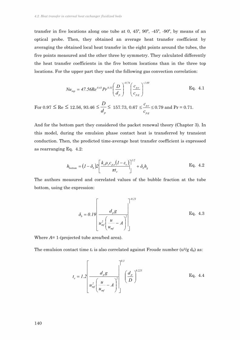
4.2. Heat transfer in external heat exchanger fluidized beds
140
transfer in five locations along one tube at 0, 45º, 90º, -45º, -90º, by means of an
optical probe. Then, they obtained an average heat transfer coefficient by
averaging the obtained local heat transfer in the eight points around the tubes, the
five points measured and the other three by symmetry. They calculated differently
the heat transfer coefficients in the five bottom locations than in the three top
locations. For the upper part they used the following gas convection correlation:
1.69
gp,
sp,
0.74
p
0.330.43top c
c
d
DPr47.56ReNu
Eq. 4.1
For 0.97 Re 12.56, 93.46 pd
D 157.73, 0.67
gp,
sp,
c
c0.79 and Pr = 0.71.
And for the bottom part they considered the packet renewal theory (Chapter 3). In
this model, during the emulsion phase contact heat is transferred by transient
conduction. Then, the predicted time-average heat transfer coefficient is expressed
as rearranging Eq. 4.2:
gb
1/2
e
eep,sebbottom hδ
πt
ε1cρk2δ1h
Eq. 4.2
The authors measured and correlated values of the bubble fraction at the tube
bottom, using the expression:
-0.23
2
mf
2mf
pb
Au
uu
gd0.19δ
Eq. 4.3
Where A= 1-(projected tube area/bed area).
The emulsion contact time te is also correlated against Froude number (u2/g dp) as:
0.225
p
0.3
2
mf
2mf
pe D
d
Au
uu
gd1.2t
Eq. 4.4

Chapter 4. The influence of solids recirculation on heat transfer in an external heat exchanger
141
So, they finally proposed an expression averaging both terms, the heat transfer
coefficient in the denser bottom part of the tube, hbottom, and the heat transfer
coefficient in the top, htop:
topbottomave h8
3h
8
5h Eq. 4.5
Their findings coincide with the ones by Ozawa (1998), obtaining maximum heat
transfer at the side of the tube and minimum at the top, down to 200 W/m2K for
fluidizing velocities around minimum fluidizing velocity. Maximum heat transfer
was observed for velocities around twice the minimum fluidizing velocity, reaching
values of 450 W/m2K.
4.2.2 INFLUENCE OF SOLIDS RECIRCULATION
The movement of solids in the horizontal direction of a fluidized bed could be
neglected compared with the vertical movement of solids. This difference could be
expressed in terms of the vertical and horizontal dispersion coefficients. With the
aim of acquiring an idea of the magnitude of these terms, following, Figure 4.2
represents both dispersion coefficients versus the ratio of velocities.
Figure 4.2. Dispersion coefficients calculated for different fluidization velocities and
different tubes arrangements, according to Eq. 4.6 and Eq. 4.7.
2 3 4 5 6 7 8
x 10-3 x 10-1
0
0,05
0,1
0,15
0,2
0,25
0,3
0,35
0,4
0,45
0
0,1
0,2
0,3
0,4
0,5
0,6
0,7
0,8
uf/umf
Ds
h (
m2/s
)
0.025 m 0.025 m
0.15 m 0.15 m
0.3 m 0.3 m
0.5 m 0.5 mpinch
Ds
v (
m2/s
)
DsvDsh

4.2. Heat transfer in external heat exchanger fluidized beds
142
The dispersion coefficients shown in Figure 4.2 have been calculated according to
Kunii and Levenspiel (1991) proposal. The horizontal dispersion coefficient, Dsh,
yields:
mf
bmf2
b
bsh ε
duα
δ1
δ
16
3D Eq. 4.6
α is the ratio between the wake size and the bubble size. It is recommended α=1 for
small Geldart A and AB particles and α=0.77 for larger solids.
The vertical dispersion coefficient, Dsv, is expressed as:
mf
2b
bmf2
wsv 3u
uδdεfD Eq. 4.7
In this expression fw represents the fraction of wakes according to the counterblow
solid circulation model (Kunii and Levenspiel, 1991). Values for this term would be
between 0.3 and 2.
As seen in the Figure 4.2 tendencies of both terms are similar for different
distances between tubes, but vertical dispersion coefficient is two orders of
magnitude greater than the horizontal term, what makes it possible to neglect it in
most of cases.
As mentioned before, heat transfer surfaces immersed in dense fluidized bed are
particularly important in external heat exchangers of circulating fluidized beds. In
these devices particles not only move in one direction but they must be conveyed
along the heat exchanger to reach the solids recycling pipe. Consequences of this
additional dimension have been scarcely studied and it will play an essential role
for the next generation of oxy-fuel fluidized bed combustors.
With the aim of observing such effects of recycled solids on the heat transfer in an
external heat exchanger, Wang and co-workers (2003) designed a cold model of
loop-seal with external heat exchanger. The solids rate was controlled by diverting
part of the particles from the standpipe by changing fluidizing velocity of both,
loop-seal and external heat exchanger. Heat transfer probes were located in
different positions in the external heat exchanger. The results are shown in Figure
4.3:

Chapter 4. The influence of solids recirculation on heat transfer in an external heat exchanger
143
Figure 4.3. Results from the heat transfer measurement in a cold model of an External Heat
Exchanger. Adapted from Wang et al. (2003)
Heat transfer is not uniform in each location of Figure 4.3. This confirms the
influence of fluid-dynamics and tubes location on heat transfer. The maximum heat
transfer coefficients are obtained in locations 2 and 1, the central tube and the
point near the splash zone respectively. Lower and similar coefficients are obtained
in positions 3, 4 and 5, near the walls and the distributor plate. Increasing the
solids rate crossing the heat exchanger they observed higher heat transfer
coefficients, particularly in position 1 and 2. Difference between the maximum and
minimum heat transfer surfaces were almost of 45%. This indicated insufficient
fluidization areas with poor gas-solids mixing near the wall and near the
distributor plate.
Johansson et al. (2006) they studied a 1/3 scale cold model of an existing loop-seal
with immersed tubes bundle. The aim of the work was twofold: analyzing the
performance of the sealing, by measuring the solids in the down-comer and the
pressure drop across the seal and measuring heat transfer coefficient in different
locations along the loop-seal. They were able to compare their findings with the
EHE of a commercial scale CFB. Results of their experiments are plotted in Figure
4.4:
1
2
3
5 4
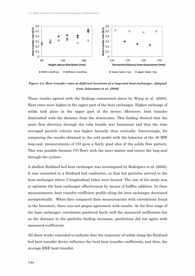
4.2. Heat transfer in external heat exchanger fluidized beds
144
Figure 4.4. Heat transfer rates at different locations of a loop-seal heat exchanger. Adapted
from Johansson et al. (2006)
These results agreed with the findings commented above by Wang et al. (2003).
Heat rates were higher in the upper part of the heat exchanger. Higher exchange of
solids took place in the upper part of the device. Moreover, heat transfer
diminished with the distance from the downcomer. This finding showed that the
main flow direction through the tube bundle was horizontal and that the time
averaged particle velocity was higher laterally than vertically. Interestingly, for
comparing the results obtained in the cold model with the behavior of the 30 MW
loop-seal, measurements of CO gave a fairly good idea of the solids flow pattern.
This was possible because CO flows with the inert matter and enters the loop-seal
through the cyclone.
A shallow fluidized bed heat exchanger was investigated by Rodriguez et al. (2002).
It was connected to a fluidized bed combustor, so that hot particles arrived to the
heat exchanger where 5 longitudinal tubes were located. The aim of the study was
to optimize the heat exchanger effectiveness by means of baffles addition. In their
measurements, heat transfer coefficient profile along the heat exchanger decreased
asymptotically. When they compared their measurements with correlations found
in the literature, there was not proper agreement with results. At the first stage of
the heat exchanger, correlation predicted fairly well the measured coefficients but
as the distance to the particles feeding increases, predictions did not agree with
measured coefficients.
All these works coincided to indicate that the trajectory of solids along the fluidized
bed heat transfer device influence the local heat transfer coefficients, and thus, the
average EHE heat transfer.
0
0,1
0,2
0,3
0,4
0,5
0,6
80 130 180
Heat trasnfer rate (K/s)
Height above distributor (mm)
With crossflow Without crossflow
0
0,1
0,2
0,3
0,4
0,5
0,6
120 170 220 270
Heat trasnfer rate (K/s)
Horizontal distance from downcomer (mm)
lower tubes row upper tubes row

Chapter 4. The influence of solids recirculation on heat transfer in an external heat exchanger
145
4.2.3 REAL EXTERNAL HEAT EXCHANGERS
There are few public data about heat transfer in real external fluidized bed heat
exchangers. In some cases, this could be due probably to confidentiality issues, but
in general, the access to the devices is usually obstructed by other components of
the plant and, particularly in heat exchangers, inserting probes involves high risk
of damaging tubes bundles.
One of the most complete studies focused on the fluid-dynamics and heat transfer
in a real loop-seal heat exchanger was the one carried out by Werdermann and
Werther (1993) in an existing BFB EHE of 10 m long and 3 m wide and 5 m height.
A heat transfer probe was used to measure heat transfer at eleven different ports
in the first chamber. Unfortunately, this was the chamber with no heat exchanger
tubes because introducing the probe in the other chambers was considered too
risky. Still, important findings were drawn from the study. Non-uniformities in the
temperature profiles were detected in the first chamber. This was attributed to the
reaction of the unburned carbon in the ash, when contacting with oxygen from
fluidizing air.
They measured heat transfer coefficients at two different distances from the front
wall and at three different heights from the distributor. Maximum heat transfer
was measured in the position further from the front wall at 0.322 m, reaching
values around 1600 W/m2K at the row near the distributor, but far from both side
walls. In the same position but at 0.114 m from the wall, the heat transfer
coefficients were only around 250 W/m2K.
When the heat transfer probe was introduced from the top of the chamber, at the
height near the limit of the bed, at 3.468 m, heat transfer was between 500 W/m2K
and 1000 W/m2K, whereas at higher position than this, heat transfer coefficient
decreases down to 100 - 550 W/m2K.
Results obtained in this study are represented in Figure 4.5:
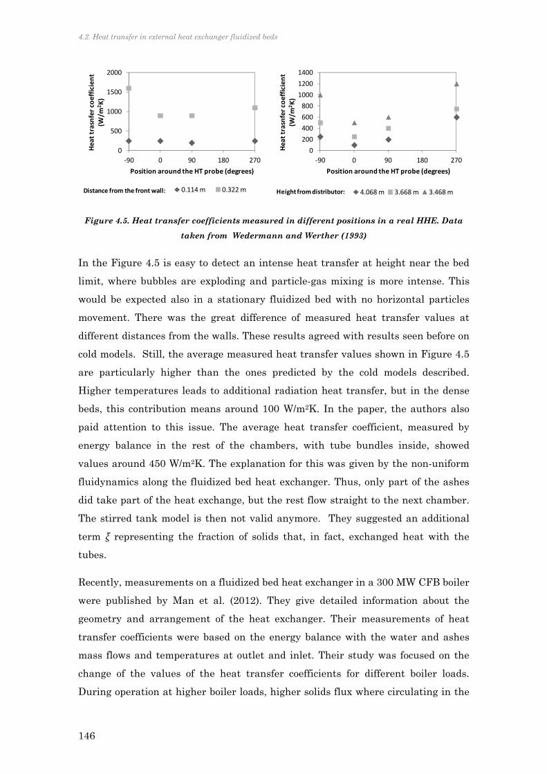
4.2. Heat transfer in external heat exchanger fluidized beds
146
Figure 4.5. Heat transfer coefficients measured in different positions in a real HHE. Data
taken from Wedermann and Werther (1993)
In the Figure 4.5 is easy to detect an intense heat transfer at height near the bed
limit, where bubbles are exploding and particle-gas mixing is more intense. This
would be expected also in a stationary fluidized bed with no horizontal particles
movement. There was the great difference of measured heat transfer values at
different distances from the walls. These results agreed with results seen before on
cold models. Still, the average measured heat transfer values shown in Figure 4.5
are particularly higher than the ones predicted by the cold models described.
Higher temperatures leads to additional radiation heat transfer, but in the dense
beds, this contribution means around 100 W/m2K. In the paper, the authors also
paid attention to this issue. The average heat transfer coefficient, measured by
energy balance in the rest of the chambers, with tube bundles inside, showed
values around 450 W/m2K. The explanation for this was given by the non-uniform
fluidynamics along the fluidized bed heat exchanger. Thus, only part of the ashes
did take part of the heat exchange, but the rest flow straight to the next chamber.
The stirred tank model is then not valid anymore. They suggested an additional
term ξ representing the fraction of solids that, in fact, exchanged heat with the
tubes.
Recently, measurements on a fluidized bed heat exchanger in a 300 MW CFB boiler
were published by Man et al. (2012). They give detailed information about the
geometry and arrangement of the heat exchanger. Their measurements of heat
transfer coefficients were based on the energy balance with the water and ashes
mass flows and temperatures at outlet and inlet. Their study was focused on the
change of the values of the heat transfer coefficients for different boiler loads.
During operation at higher boiler loads, higher solids flux where circulating in the
0
500
1000
1500
2000
‐90 0 90 180 270
Heat trasnfer coefficient
(W/m
2K)
Position around the HT probe (degrees)
0.114 m 0.322 mDistance from the front wall:
0
200
400
600
800
1000
1200
1400
‐90 0 90 180 270
Heat trasnfer coefficient
(W/m
2K)
Position around the HT probe (degrees)
4.068 m 3.668 m 3.468 mHeight from distributor:

Chapter 4. The influence of solids recirculation on heat transfer in an external heat exchanger
147
solids loop. This is analogous to the increase of fuel input when increasing O2
concentration at inlet, as resulted in Chapter 2 simulations. Results of these
measurements are shown in Figure 4.6.
Figure 4.6. Heat transfer coefficients measured in one of the chambers of the external heat
exchanger. Data taken from Man et al. (2012).
They found a direct relation between the solids rate arriving at the external heat
exchanger and the heat transfer coefficient. They proposed a simple correlation
taken into account both, the solids flux and the bed temperature, for estimating the
changes of heat transfer coefficients at different boiler loads.
38.10.12T0.8mh insolids,solidsEHE Eq. 4.8
These results can be explained also by the model suggested by Werdermann and
Werther (1993). They considered a ratio of solids that effectively exchanged heat
with the water tubes, based on the solids and water temperature, on the tubes
geometry and conductivity, and, particularly, on the heat transfer coefficients
measured in the chamber with tubes and in the first chamber with no tubes. The
expression yielded:
waterwaterinsolids,*insolids,
outsolids,insolids,
TTTh
hT
TTζ
Eq. 4.9
with
1
oi
oo
maxi
o
h
1
d
dln
2k
d
hd
dh
Eq. 4.10
4.3. Experimental set-up
148
1
1i
oo
maxi
o
h
1
d
dln
2k
d
hd
dh
* Eq. 4.11
They considered maximum heat transfer coefficient, hmax, of 1000 W/m2K in the
first chamber, with no tubes, and an average heat transfer coefficient of 750 W/m2K
in the same chamber, h0. The term h1 was the average heat transfer coefficient in
the chamber with tubes bundles, measured indirectly by energy balance, having a
value of 400 W/m2K.
From the Eq. 4.9 to Eq. 4.11 it seems no relation between the mass flow and the
heat transfer coefficients, being no dependent directly on this parameter.
However, if the term remains constant, when incrementing solids flux, the flow of
solids effectively exchanging heat with tubes also increases, which actually can be
a plausible explanation for the effects of mass flow seen in Figure 4.6. Thus, the
simple expression in Eq. 4.8 proposed by Man et al. (2012) can actually represent
also this effect.
The relevance of the EHE on the energy balance of future CFB will reside
predominantly on the increasing flow of recycled solids compared with the air-
firing case. The available literature reviewed on the cold models revealed an un-
even distribution of heat transfer along the EHE tubes bundle. In real EHE, the
average heat transfer coefficient was also dependant on the mass flow of solids
crossing the EHE. The following experimental campaign aims at looking for the
relation between both effects, particularly for a wide range of solids mass flow rate.
4.3 EXPERIMENTAL SET-UP
The loop-seal heat exchanger cold model used by Johansson et al. (2006) in their
work was un-coupled from the original two dimensional CFB set up. This allowed
operating the loop-seal independently from the CFB operational parameters. The
scheme is represented in Figure 4.7 and Figure 4.8 shows the photo of the
arrangement.
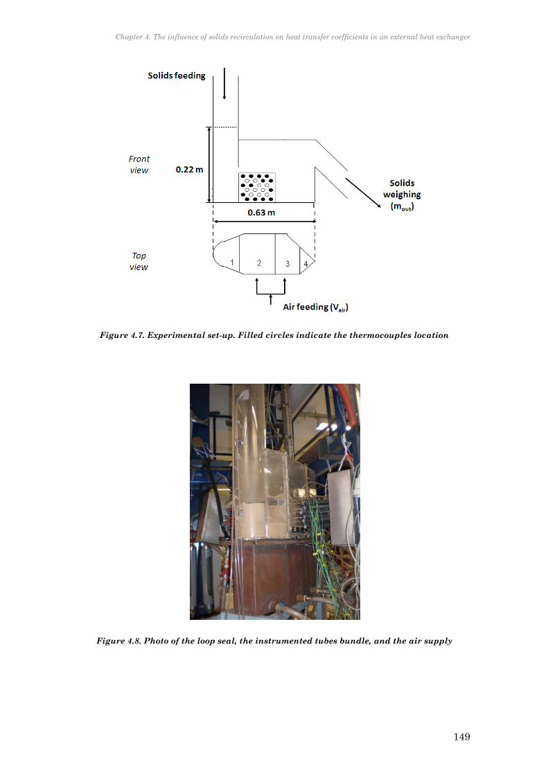
Chapter 4. The influence of solids recirculation on heat transfer coefficients in an external heat exchanger
149
Figure 4.7. Experimental set-up. Filled circles indicate the thermocouples location
Figure 4.8. Photo of the loop seal, the instrumented tubes bundle, and the air supply

4.3 Experimental set-up
150
The EHE is located in the Chalmers University of Technology. It consists of a
Plexiglas loop-seal, with 24 copper tubes crossing horizontally. Solids were fed from
the top of the down-comer. After traveling along the loop-seal, they arrived to the
recycling pipe, originally attached to the bottom zone of the CFB. Solids from the
recycling pipe were weighted for estimating an average flow rate of solids in every
test. Air entered directly to the chambers 2 and 3 through perforated plates. A
rotameter flow-meter with a manual globe valve allowed varying de fluidizing gas
velocity. Tap warm water circulated inside the tubes, reaching a maximum
temperature around 40ºC. 15 of the 24 tubes (filled circles in Figure 4.7) had
attached thermocouples in the surface. The water temperature was approximately
that of the tubes, because of the high conductivity of copper.
Once the water circulation stoped, we estimated the cooling rates in each tube with
the following expression:
12
12
tt
TT
Δt
ΔT
Eq. 4.12
Capital letters represent temperature in the moment t2 and t1 respectively. Figure
4.9 displays a typical cooling curve and the initial 10 seconds that were used for the
cooling rate estimation.
Figure 4.9. Example of cooling curve for a testing tube. Zoom to the first seconds of cooling
to calculate the cooling rate.
35
36
37
38
39
40
41
335 350 365 380 395 410 425 440 455 470 485
Tube 9 temperature (ºC)
Time (s)
38
39
40
345 350 355 360 365
Time (s)∆t
∆T

151
In order to compare the influence of solids recirculation on the heat transfer
performance in the loop-seal, the mass flow fed by the dip-leg was widely varied.
Thanks to the un-coupling with the overall CFB arrangement, the solids rate could
vary within a wide range of values. On the other hand, this uncoupling, did not
permit a good regulation of solids feed, particularly at high rates. These ranges are
presented in Table 4.1. The fluidizing velocity was kept below 5 umf, in order to
avoid the return of gas trough the dip-leg.
mout (kg/s) u/umf planned achieved planned achieved
0 0 0 0 1 1.2-1.5
0-5 0.8-4.7 1-3 2-3 3-5 3.6
5-15 5.3-13.5 1-3 2.4-2.8 3-5 3.6-4.8
15-30 15-23.4 1-3 1-2.8 3-5 3.2
>30 30-71.8 1-3 1.6-3 3-5 3.6
Table 4.1. Experiments planning matrix for the operation of the cold EHE
The cooling rate in every tube was measured. The tubes with attached
thermocouples are widespread among the tube bundle. They provided information
at different locations in the loop-seal: along height and from the dip-leg to the
recycling pipe area.
4.4 RESULTS OF HEAT TRANSFER IN THE COLD EHE
4.4.1 COOLING RATES
The cooling rates are negative values, because of the sign of the calculated slope.
This is, the further the cooling, the more negative the cooling rate value, and the
higher the heat transfer in that position. We can so identify the conditions at which
cooling are uneven distributed along the tubes. In order to easier visualize the
cooling rates results, in the following graphs, these are represented against the
tubes position in the horizontal distance from the down-comer. Figure 4.10
illustrates three cases for the first row of tubes, one with no solids feeding crossing
the EHE, and two different solids flow, 7 kg/s and 8.7 kg/s, respectively.

4.4. Results on heat transfer in the cold EHE
152
Figure 4.10. Cooling rates at the first row, near the distributor, low velocities
The case of no solids feeding presents uniform cooling rates along the loop-seal, and
the lowest values out from the three cases. When solids are fed and fluidizing
velocity increases, more intense cooling takes place far from the downcomer. The
values showed that uniformity of cooling observed in the reference case, is
disturbed when solids cross the EHE. These observations agree with the previous
findings, in which the trajectory shaped by solids influenced heat transfer
coefficients at the different locations.
In Figure 4.11 and Figure 4.12, cooling rates are represented in the lowest (1st) and
highest (6th) tubes positions. Figure 4.11 shows the reference case with no solids
feeding (the same as in Figure 4.10), and two cases with different mass and air
flows: 4.7 kg/s with 3umf m/s, and 15 kg/s with 4umf m/s. Here, the increase of
cooling rates is also higher in the cases with solids feeding, compared with the
reference case. Interestingly, a markedly inequality is shown by the case of
medium air velocity and solids flow, doubling the value of cooling rate near the
down-comer. With highest solids flow, cooling rates are more uniform, particularly
in the 6th row.

Chapter 4. The influence of solids recirculation on heat transfer coefficients in an external heat exchanger
153
Figure 4.11. Comparison between low and higher tubes with two solid rates
Figure 4.12 shows two cases, with low solids rate and different fluidizing velocities,
together with the reference case with no solids feeding. On this occasion the cooling
is slightly higher in the case with higher aeration velocity and this is also the
conditions at which inequalities at different positions are increased.
Figure 4.12. Comparison between low and higher tubes with two aeration velocities
Unlike in Figure 4.11, in Figure 4.12 the distribution of cooling along the tubes in
the 1st row for the highest velocity case is more even. The major cooling occurs in
the last row, in the tubes near the down-comer, and it diminishes with the
distance.
Up to here, the influence of fluidizing velocity on the cooling rate turns
predominant over the mass flow of solids traveling across the EHE. However, heat
transfer is increased when solids travel through the EHE. The uneven cooling
among the tubes must be due to the different distribution of warm solids at the
different locations in the EHE. This is related to the combination of the fluidizing
‐0.12
‐0.10
‐0.08
‐0.06
‐0.04
‐0.02
0.00
0 2 4 6 8 10Cooling rate (K/s)
Tubes column position from the down‐comer
1st row
a)
‐0.12
‐0.10
‐0.08
‐0.06
‐0.04
‐0.02
0.00
0 2 4 6 8 10
Cooling rate (K/s)
Tubes column position from the down‐comer
6th row
b)
u/umf=1.5; m=0 kg/s u/umf=3; m=4.73 kg/s u/umf=4; m=15 kg/s
‐0.12
‐0.10
‐0.08
‐0.06
‐0.04
‐0.02
0.00
0 2 4 6 8 10
Cooling rate (K/s)
Tubes column position from the down‐comer
1st row
a)
‐0.12
‐0.10
‐0.08
‐0.06
‐0.04
‐0.02
0.00
0 2 4 6 8 10
Cooling rate (K/s)
Tubes column position from the down‐comer
6th row
b)
u/umf=1.5; m=0 kg/s u/umf=2; m=3 kg/s u/umf=3.6; m=3.21 kg/s
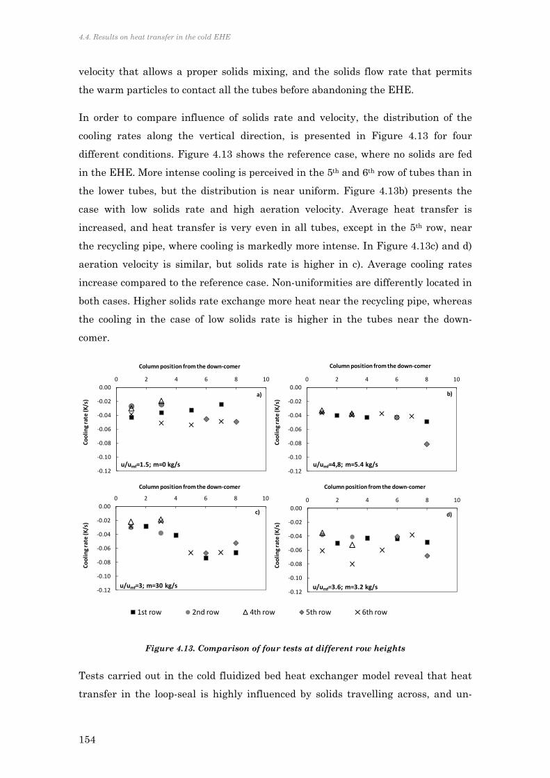
4.4. Results on heat transfer in the cold EHE
154
velocity that allows a proper solids mixing, and the solids flow rate that permits
the warm particles to contact all the tubes before abandoning the EHE.
In order to compare influence of solids rate and velocity, the distribution of the
cooling rates along the vertical direction, is presented in Figure 4.13 for four
different conditions. Figure 4.13 shows the reference case, where no solids are fed
in the EHE. More intense cooling is perceived in the 5th and 6th row of tubes than in
the lower tubes, but the distribution is near uniform. Figure 4.13b) presents the
case with low solids rate and high aeration velocity. Average heat transfer is
increased, and heat transfer is very even in all tubes, except in the 5th row, near
the recycling pipe, where cooling is markedly more intense. In Figure 4.13c) and d)
aeration velocity is similar, but solids rate is higher in c). Average cooling rates
increase compared to the reference case. Non-uniformities are differently located in
both cases. Higher solids rate exchange more heat near the recycling pipe, whereas
the cooling in the case of low solids rate is higher in the tubes near the down-
comer.
Figure 4.13. Comparison of four tests at different row heights
Tests carried out in the cold fluidized bed heat exchanger model reveal that heat
transfer in the loop-seal is highly influenced by solids travelling across, and un-
‐0.12
‐0.10
‐0.08
‐0.06
‐0.04
‐0.02
0.00
0 2 4 6 8 10
Cooling rate (K/s)
Column position from the down‐comer
a)
u/umf=1.5; m=0 kg/s
‐0.12
‐0.10
‐0.08
‐0.06
‐0.04
‐0.02
0.00
0 2 4 6 8 10
Cooling rate (K/s)
Column position from the down‐comer
u/umf=3; m=30 kg/s
c)
‐0.12
‐0.10
‐0.08
‐0.06
‐0.04
‐0.02
0.00
0 2 4 6 8 10
Cooling rate (K/s)
Column position from the down‐comer
b)
u/umf=4,8; m=5.4 kg/s
‐0.12
‐0.10
‐0.08
‐0.06
‐0.04
‐0.02
0.00
0 2 4 6 8 10
Cooling rate (K/s)
Column position from the down‐comer
u/umf=3.6; m=3.2 kg/s
d)
1st row 2nd row 4th row 5th row 6th row

Chapter 4. The influence of solids recirculation on heat transfer coefficients in an external heat exchanger
155
uniformities of heat transfer coefficients along the loop-seal are caused by the
trajectory of these solids in their way to the recycled pipe. Heat transfer near the
bed limit is more intense. Higher velocities could allow better solids mixing and
hence, would reduce differences on heat transfer from one area to another in the
loop-seal.
Up to this points we can conclude that high flows of solids arriving at the loop-seal
EHE enhances heat transfer. However, the un-even distribution of tubes cooling is
caused by this flow of solids. The non-uniformities are also related to adequate
aeration velocities that allow proper mixing of solids. This translates into that
maximum cooling rates were not found for the case of highest velocity and highest
solids rate.
The local cooling rates measured in the previous experiments will be used to
following calculate the local heat transfer coefficients in each tube.
4.4.2 UNEVEN DISTRIBUTION OF HEAT TRANSFER COEFFICIENTS
Cooling rates previously presented are a transient heat transfer process (Mills,
1995). The heat exchange between tubes and bed, Q, can be written as:
dt
dTCVCVTThAQ wwwCuCuCuBHT
Eq. 4.13
The CuCuCu CpV and www CpV terms are the lumped thermal capacitance of copper
and water respectively. AHT is the surface of tubes available for heat exchange. TB
indicates the value of the bulk of particles. Rearranging Eq. 4.13, the heat transfer
coefficient in each tube yields:
)( bHT
iwwwCuCuCu
iTTA
tTCpVCpV
h
Eq. 4.14
Where index i represents the coefficient and temperature at each tube. Tubes
diameter were 1/4” and cupper density and specific thermal capacity were 8932
kg/m3 and 0.3854 kJ/kgK, respectively.
Following the heat transfer coefficient will be displayed against the horizontal
position from the downcomer of the respective tube. In Figure 4.14a) and b),
different solids rates are represented, for low and high aeration velocity,

4.4. Results on heat transfer in the cold EHE
156
respectively. In Figure 4.14a) two cases are represented, in which the ratio u/umf is
4.8 and the solids rate is 2.4 and 5.4 kg/s. The case with lower solids rate present
also lower heat transfer values. Moreover, uneven distribution of heat transfer is
more evident in the lower solids rate case, with a variation around 80%.
In Figure 4.14b) solids rate varies from 22.7 and 8.7 kg/s, with lower velocity ratio,
2.8. In this cases, the inequalities in the heat transfer values is up to four times the
minimum values in the position near the down-comer, and even higher close to the
recycling pipe.
Figure 4.14. Heat transfer coefficients, a) high velocity and increasing solids rate; b) low velocity and different solids rate
Figure 4.14 reveals that aeration velocity and solids rate must be adequately
related in order to obtain not only high heat transfer coefficients, but optimum
distribution among the heat exchanger tubes. Another example of this affirmation
is shown in Figure 4.15. They are represented the cases with lowest fluidizing
a)
b)

Chapter 4. The influence of solids recirculation on heat transfer coefficients in an external heat exchanger
157
velocity and a considerable amount of solids traveling through the EHE, and a
higher velocity ratio with less solids rate. The average heat transfer coefficient is,
in both cases, around 100 W/m2K, although the higher solids rate induces further
inequalities in the heat transfer among the tubes.
Figure 4.15. Heat transfer coefficients with two velocities and solids rate conditions
Increasing aeration velocity would lead to higher gas flow in the chamber 3.
Pressure drop in this chamber is lower than in chamber 2, because no tubes are
present. Then, certain reflux of aeration gas could have intensified cooling rates of
last tubes columns. However, in the experiments where aeration velocity was as
high as 4.8 times the minimum fluidizing velocity, heat transfer coefficients
distribution kept uniform. The dominant cause of dissimilarities of heat transfer
lied on the increment of Gs.
In the conventional operation of an EHE, the different heat transfer coefficients at
different tubes locations are not usually considered for the design, but the average
heat transfer coefficient. The average heat transfer coefficient among the local
values previously obtained, will allow establishing a relationship between Gs and
heat transfer coefficient, to account for the enhancement of heat transfer due to
solids recycling, in spite of dissimilarities of heat transfer among the tubes.
However, since elutriated solids rate of an oxy-fuel CFB are expected to
considerably increase, a specific design of tubes bundle will be desirable for
optimum design of future EHE. This should be carefully considered and it will be
propose as future work at the end of this document.
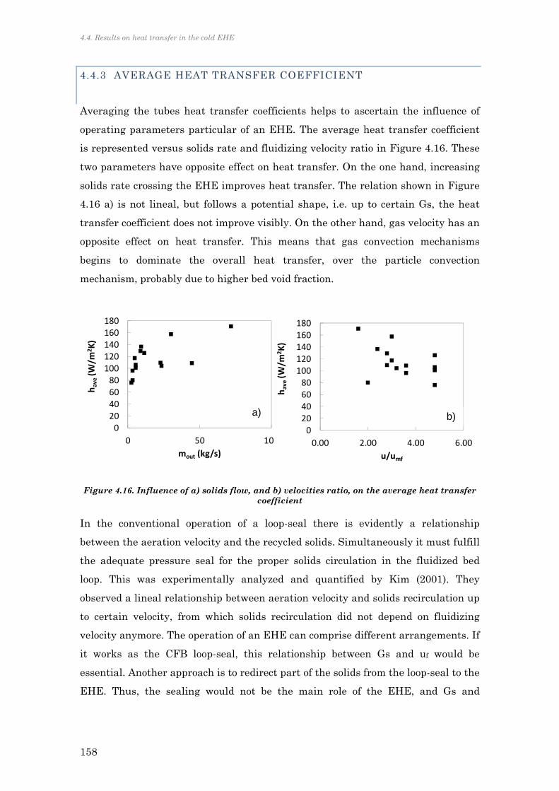
4.4. Results on heat transfer in the cold EHE
158
4.4.3 AVERAGE HEAT TRANSFER COEFFICIENT
Averaging the tubes heat transfer coefficients helps to ascertain the influence of
operating parameters particular of an EHE. The average heat transfer coefficient
is represented versus solids rate and fluidizing velocity ratio in Figure 4.16. These
two parameters have opposite effect on heat transfer. On the one hand, increasing
solids rate crossing the EHE improves heat transfer. The relation shown in Figure
4.16 a) is not lineal, but follows a potential shape, i.e. up to certain Gs, the heat
transfer coefficient does not improve visibly. On the other hand, gas velocity has an
opposite effect on heat transfer. This means that gas convection mechanisms
begins to dominate the overall heat transfer, over the particle convection
mechanism, probably due to higher bed void fraction.
Figure 4.16. Influence of a) solids flow, and b) velocities ratio, on the average heat transfer coefficient
In the conventional operation of a loop-seal there is evidently a relationship
between the aeration velocity and the recycled solids. Simultaneously it must fulfill
the adequate pressure seal for the proper solids circulation in the fluidized bed
loop. This was experimentally analyzed and quantified by Kim (2001). They
observed a lineal relationship between aeration velocity and solids recirculation up
to certain velocity, from which solids recirculation did not depend on fluidizing
velocity anymore. The operation of an EHE can comprise different arrangements. If
it works as the CFB loop-seal, this relationship between Gs and uf would be
essential. Another approach is to redirect part of the solids from the loop-seal to the
EHE. Thus, the sealing would not be the main role of the EHE, and Gs and
020406080
100120140160180
0 50 100
have(W
/m2K)
mout (kg/s)
020406080
100120140160180
0.00 2.00 4.00 6.00
have(W
/m2K)
u/umf
a) b)
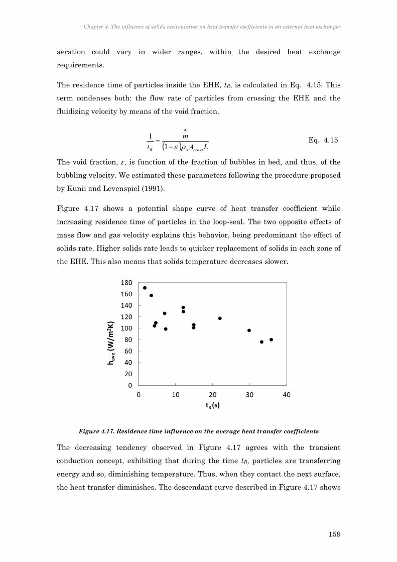
Chapter 4. The influence of solids recirculation on heat transfer coefficients in an external heat exchanger
159
aeration could vary in wider ranges, within the desired heat exchange
requirements.
The residence time of particles inside the EHE, tR, is calculated in Eq. 4.15. This
term condenses both: the flow rate of particles from crossing the EHE and the
fluidizing velocity by means of the void fraction.
LA
m
t crosssR
1
1 Eq. 4.15
The void fraction, ε, is function of the fraction of bubbles in bed, and thus, of the
bubbling velocity. We estimated these parameters following the procedure proposed
by Kunii and Levenspiel (1991).
Figure 4.17 shows a potential shape curve of heat transfer coefficient while
increasing residence time of particles in the loop-seal. The two opposite effects of
mass flow and gas velocity explains this behavior, being predominant the effect of
solids rate. Higher solids rate leads to quicker replacement of solids in each zone of
the EHE. This also means that solids temperature decreases slower.
Figure 4.17. Residence time influence on the average heat transfer coefficients
The decreasing tendency observed in Figure 4.17 agrees with the transient
conduction concept, exhibiting that during the time tR, particles are transferring
energy and so, diminishing temperature. Thus, when they contact the next surface,
the heat transfer diminishes. The descendant curve described in Figure 4.17 shows
0
20
40
60
80
100
120
140
160
180
0 10 20 30 40
have(W
/m2 K)
tR (s)

4.4. Results on heat transfer in the cold EHE
160
that, in the extreme case in which tR is infinite, the heat transfer set in a constant
value. This is the case in which no solids were recycled.
The average heat transfer coefficients and residence times of recycled solids
obtained for the cold model are now represented in the dimensionless form, Н and
Θ, respectively. This allows including the values measured in a real EHE, reported
by Man et al. (2012), and previously explored. Figure 4.18 displays results from
both, the cold model and the real EHE, in dimensionless form. The values follow a
decreasing potential shape that stabilized in the minimum heat transfer
coefficient. This minimum heat transfer coefficient will approach the value in
which solids are not crossing the EHE, i.e. there is not lateral flow of warm solids.
The curve that fits the values in Figure 4.18 is correlated by the expression
(R2=0.65):
322073242 .Θ.Η Eq. 4.16
Eq. 4.16 allows modifying the heat transfer coefficient estimated for non recycled
solids conditions, and estimating how much this coefficient is enhanced by the
solids flow traveling through the EHE.
Figure 4.18. Influence of residence time of recycled particles on heat transfer coefficients in the cold model and in the real EHE
0.0
0.5
1.0
1.5
2.0
2.5
3.0
3.5
4.0
4.5
0 5 10 15 20 25
Н
Θ
This study
Man et al. (2012)

Chapter 4. The influence of solids recirculation on heat transfer coefficients in an external heat exchanger
161
With the expression proposed in Eq. 4.16 accounting for the influence of Gs on
heat transfer, and the heat transfer semi-empirical approach deduced in last
chapter, Eq. 3.34, we are ready to extrapolate these expressions to the sub-model of
an EHE to include it in the modeling of the large CFB boiler.
4.5 INTEGRATION OF THE EHE MODEL IN THE OXY-FUEL
CFB MODEL
4.5.1 FLY-ASH RE-CARBONATION
Before developing the sub-model of the external heat exchanger fluidized bed, a
relevant issue, particular of oxy-fuel operation, must be addressed. This is the
possibility that re-carbonation of fly ashes, coming from the cyclone, takes place in
the EHE. Under oxy-firing conditions, conventional bed temperature is not high
enough to allow limestone calcination and direct sulfation takes place. This was
further addressed in section 2.2.2. This leads to a decrease of SO2 capture efficiency
compared to indirect sulfation using the same calcium to sulfur ratio.
Higher bed temperature can be a solution for reaching similar SO2 capture
efficiency during oxy-fuel combustion. In this case, limestone is calcined yielding
large amount of CaO. Sulfation process occurs in the particles surface, until
external pores are blocked by CaSO4 layer. Diffusion to the CaO core is then
difficult for SO2. Thus, an excess of Ca:S over stoichiometric is necessary for
assuring proper SO2 capture. Still, considerably CaO surface is available after
travelling along the riser.
Conventional temperature in the external heat exchanger ranges between 750ºC-
650ºC (Nsakala et al., 2004) and these are the temperature values obtained for
proper bed temperature in the previous analysis. At this temperature and high CO2
partial pressure, CaO tends to quickly re-carbonate. Then, if calcination had been
taken place, large amount of CaO would arrive to the loop-seal. In oxy-firing
conditions, loop-seal is fluidized with CO2 or RFG that can easily react with the
available CaO. In Figure 4.19 CaO-CaCO3 equilibrium is represented and
conditions in boiler and loop-seal are indicated. It can be distinguished that
conditions at which a loop-seal works are clearly in the carbonation area. The

4.5. Integration of the EHE model in the oxy-fuel CFB model
162
optimum air-firing temperature is also marked and calcination is not likely to occur
under high CO2 partial pressure proper of oxy-fuel combustion.
Figure 4.19. Carbonation-calcination equilibrium
With the aim of exploring the influence of direct and indirect sulfation on the CaO
rate reaching the EHE, the CFB model developed in Chapter 2 is now run, for two
temperature levels, and two oxygen concentrations. Figure 4.20 illustrates the
results at 850ºC and 900ºC, with the 40% O2 concentrations in the oxidant stream.
Figure 4.21 graphs simulations results when feeding 60% O2 at the same two
average bed temperatures. In both graphs, zoom is made on the bottom part of the
boiler, where most of reactions take place. The equilibrium pressure is represented
in bold line for both cases, according to Eq. 2.23. The higher temperature level,
around 900ºC is depicted in dotted line and the lower in discontinuous line. When
the values of CO2 partial pressure are higher than those of the equilibrium curve,
indirect sulfation occurs. The contrary happens if the partial pressure of CO2 is
lower, i.e., sulfation occurs in one step. Figure 4.21 shows that, with O2
concentration as high as 60%, direct sulfation occurs in the lower part of the boiler,
even at high temperature, which reduces the sulfation efficiency, although CaO
available in the solids loop is also lower.
500 600 700 800 900 1000 11000,001
0,01
0,1
1
5
Temperature (ºC)
CO
2 p
art
ial p
ress
ure
(at
m)
Typical LS with EHE
Expected CO2 partialpressure in the loop‐seal
Calcination
Carbonation
Optimum bedtemperature in AF
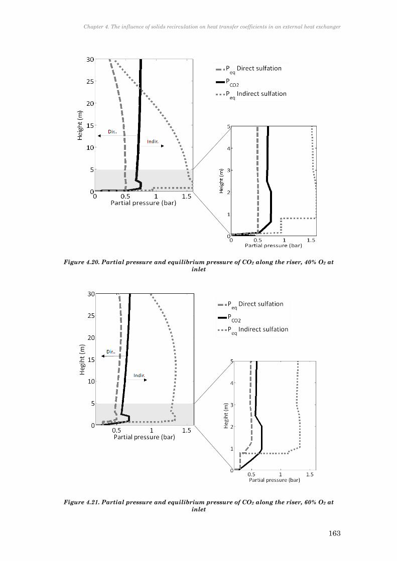
Chapter 4. The influence of solids recirculation on heat transfer coefficients in an external heat exchanger
163
Figure 4.20. Partial pressure and equilibrium pressure of CO2 along the riser, 40% O2 at inlet
Figure 4.21. Partial pressure and equilibrium pressure of CO2 along the riser, 60% O2 at inlet
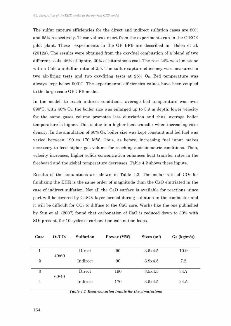
4.5. Integration of the EHE model in the oxy-fuel CFB model
164
The sulfur capture efficiencies for the direct and indirect sulfation cases are 80%
and 95% respectively. These values are set from the experiments run in the CIRCE
pilot plant. These experiments in the OF BFB are described in Bolea et al.
(2012a). The results were obtained from the oxy-fuel combustion of a blend of two
different coals, 46% of lignite, 30% of bituminous coal. The rest 24% was limestone
with a Calcium-Sulfur ratio of 2.5. The sulfur capture efficiency was measured in
two air-firing tests and two oxy-firing tests at 25% O2. Bed temperature was
always kept below 900ºC. The experimental efficiencies values have been coupled
to the large-scale OF CFB model.
In the model, to reach indirect conditions, average bed temperature was over
890ºC, with 40% O2; the boiler size was enlarged up to 3.9 m depth: lower velocity
for the same gases volume promotes less elutriation and thus, average boiler
temperature is higher. This is due to a higher heat transfer when increasing riser
density. In the simulation of 60% O2, boiler size was kept constant and fed fuel was
varied between 190 to 170 MW. Thus, as before, increasing fuel input makes
necessary to feed higher gas volume for reaching stoichiometric conditions. Then,
velocity increases, higher solids concentration enhances heat transfer rates in the
freeboard and the global temperature decreases. Table 4.2 shows these inputs.
Results of the simulations are shown in Table 4.3. The molar rate of CO2 for
fluidizing the EHE is the same order of magnitude than the CaO elutriated in the
case of indirect sulfation. Not all the CaO surface is available for reactions, since
part will be covered by CaSO4 layer formed during sulfation in the combustor and
it will be difficult for CO2 to diffuse to the CaO core. Works like the one published
by Sun et al. (2007) found that carbonation of CaO is reduced down to 30% with
SO2 present, for 10 cycles of carbonation-calcination loops.
Table 4.2. Recarbonation inputs for the simulations
Case O2/CO2 Sulfation Power (MW) Sizes (m2) Gs (kg/m2s)
1 40/60
Direct 90 3.5x4.5 10.9
2 Indirect 90 3.9x4.5 7.2
3 60/40
Direct 190 3.5x4.5 34.7
4 Indirect 170 3.5x4.5 24.5

Chapter 4. The influence of solids recirculation on heat transfer coefficients in an external heat exchanger
165
Case
Emitted
SO2a
(ppm)
Elutriated
CaCO3
(kmol/s)
Elutriated
CaO
(kmol/s)
CaO available
for carbonation
(kmol/s)
Loop-seal
fluidizing
CO2 (kmol/s)
1 1361 0.011 - - 0.0164
2 319 - 0.011 0.0033 0.0182
3 2174 0.0247 - - 0.0164
4 963 - 0.0216 0.0065 0.0164
aNormalized SO2 emissions: C-C
6-CCC
outOinO
inO
meas,OSO6%OSO
22
2
2222
Table 4.3. Recarbonation results from the simulations
For higher O2 ratios at inlet, molar flow of CaO arriving at the loop-seal is twice
the molar flow of CO2 needed for fluidization. The values obtained by Sun et al.
(2007) for estimating the available CaO surface available were considered here.
According to this paper, the factor of 0.3 is applied to the total flow of CaO arriving
to the loop-seal and indicated in the column called CaO available for carbonation.
Still, in the case of 60% O2 at inlet, de-fluidization is highly probable.
When indirect sulfation is the predominant SO2 capture phenomena, the risk of
defluidization of the loop-seal is a problem that must be tackled in this CO2 capture
technology. Particularly, when wet flue gas recirculation took place, the presence of
steam on RFG would catalyze the carbonation reaction, probably due to formation
of transient hydroxide species (Wang et al., 2008). The presence of steam would
make even more probable loop-seal defluidization than fluidizing gas without H2O.
To avoid this issue, several options could be suggested:
‐ The first choice would seem to change the fluidizing gas of the loop-seal. Air
cannot be an option, since N2 means impurities in the CO2 stream difficult
to eliminate before the CO2 compression train. Fluidizing the loop-seal with
steam would form CaO-OH, which actually enhances SO2 capture (Wang et
al., 2011). However, this compound is weaker and would favor attrition and
segregation. Moreover, consequences of such high steam content inside the
boiler must be carefully studied.
‐ Higher temperature in the loop-seal to avoid optimal conditions for the re-
carbonation is not suitable for oxy-fuel combustion. This is narrowly related
with what was demonstrated in Chpater 2, on the essential function of the

4.5. Integration of the EHE model in the oxy-fuel CFB model
166
EHE: in oxy-fuel combustion, gases entering the furnace are reduced,
compared to air-firing. To reach similar velocities, bed cross-sectional area
is decreased. Less volume means less available steam-wall surface for the
same fuel-input. Then temperature must be regulated by two additional
ways:
o Increasing solids concentration along the riser for enhancing heat
transfer coefficient by increasing solids convection. This has an
immediate effect: higher solids concentration increases wall layer
density and so, shadow effect of solids diminishes radiation to be
“seen” by the water-wall.
o Heat transferred in the loop seal to an external heat exchanger could
be intensified by further cooling of recycled particles, or by increasing
mass flow of particles crossing the loop-seal.
‐ Avoiding calcination by keeping bed temperature under direct-sulfation
conditions could be an interesting option. To reach high SO2 capture
efficiency as in indirect sulfation case, higher Ca:S ratio should be
introduced. This would lead to higher solids circulation. The additional
limestone needed means a minimum proportion to the total amount of solids
elutriated from the riser.
‐ Increasing fluidization volume gas flow rate would allow CaO to be re-
carbonated and also it would let enough CO2 for proper fluidization.
However, in practice this does not seem an easy option. The risk of either
defluidization or gas by-pass to the cyclone is too high. The difference
between the minimum CO2 flow rate needed for bubbling conditions in the
loop-sea and the total amount of CaO available for carbonation could be too
short, if there were enough carbonation capacity of the CaO particles, and
regulation would turn rather complicate.
The risk of loop-seal de-fluidization by re-carbonation of CaO has been reported
by METSO Power, occurring in their 4 MW CFB boiler (Varonen et al., 2012).
During the tests in which re-carbonation took place, limestone addition
generated circulation problems in oxy-combustion, due to the recarbonation of
CaO. In occasions, this reaction blocked the loop seal. Hence, all the circulation
material was collected into the loop seal, dipleg and cyclone, which finally led to
furnace temperature increase and sintering. They had confirmed the conditions
of re-carbonation reactions at laboratory scale (Hyytiäinen et al., 2011). They

Chapter 4. The influence of solids recirculation on heat transfer coefficients in an external heat exchanger
167
suggested that the safe operating window in oxy-mode must be defined and
recarbonation problems were avoided if the process was controlled accordingly.
Thus, the fourth option previously numbered, is the one selected for the
modeling of the EHE. If recarbonation is likely to occur, fluidizing velocity will
have to increase to prevent de-fluidization, and so, the operational window will
be adequate.
4.5.2 EXTERNAL HEAT EXCHANGER SIMULATION
The sub-model for the external heat exchanger gets results from the CFB model
developed in Chapter 2. The temperature of recycled solids was an input variable,
for assuring the required average temperature along the boiler. It was a black box
and calculation of the heat removed was calculated by energy balance with the flow
of solids and the temperature difference. Now, the aim is to go into this device in
depth. From the overall boiler simulation, data entering the EHE sub-model
include the solids entrainment, the temperature of these solids, the composition of
the flue gas, which will fluidized the EHE, and the amount of calcium-based
components from the limestone. The overall sequence of programming the EHE is
represented in Figure 4.22.
There are some external variables needed to complete the model. The geometrical
configuration of the model was based on the one described by Man et al. (2012).
They gave much detail about the arrangement of the different chambers and the
fluidizing velocity. This makes possible to draw more realistic conclusions from the
model itself. Based on this real EHE arrangement, the model is divided into three
chambers. The first one has no tubes. It is fluidized initially with 0.5 m/s and has
cross sectional area of 0.7 x 4.4 m. The second and the third chambers are the ones
containing the tubes bundles. Their cross sectional areas are 4.2 m x 4.4 m and 3.5
m x 4.4 m, respectively and they are fluidized initially with a velocity of 0.3 m/s.
Temperature of water entering the second chamber is 386ºC. The rest of
temperatures are calculated in the simulation. As initial data, the heat exchanger
effectiveness is also an input. It is an average value among those deduced from the
data given in the paper, around 0.7. This effectiveness is defined as:
water,insolids,insolidsp,solids
waterEHE TTmc
Q
Q
Qesseffectiven
max
Eq. 4.17

4.5. Integration of the EHE model in the oxy-fuel CFB model
168
Figure 4.22. Modeling flow chart of the integration of an External Heat Exchanger into the global CFB model
Initially it is assumed that all the solids falling from the cyclone are conducted to
the external heat exchanger. In the first chamber, there are no tubes, but
conditions can favored the re-carbonation of CaO present in the solids, as
previously explained. If this happens, to avoid de-fluidization, velocity must be
increased. The re-carbonation energy is included when calculating the temperature
of solids entering the second chamber.
Solids arriving at the second chamber, transfer energy to the water. The
temperature of the water at outlet is calculated by the effectiveness value, with Eq.
4.17. If recarbonation takes and the chamber de-fluidized, the velocity is
incremented, and the re-carbonation energy is included in the energy balance. This
sequence is repeated in the following chamber. Finally, temperature of solids
abandoning the EHE is calculated. If they are higher than required by the CFB
model, part of the solids bypasses the EHE and temperature of solids entering back
in the boiler is calculated by energy balance:

Chapter 4. The influence of solids recirculation on heat transfer coefficients in an external heat exchanger
169
solids,outEHEspsolids,inbypasssprequierdrecycledsp TmcTmcTmc ,,, Eq. 4.18
The solids temperature and the heat transfer coefficient will establish the required
area for reaching the specified temperature of solids. To attain the convergence, the
key variable is the fraction of solids conducted through the EHE.
4.5.3 INTEGRATION RESULTS
To take into consideration the possibility of re-carbonation of CaO in the EHE, two
different average bed temperatures in the boiler will be considered, to explore the
model results. One of these temperatures will be high enough to form CaO in the
boiler. This way, we could observe the increase on the fluidizing velocity in the
EHE to cope with de-fluidization. The other temperature will be less than 900ºC,
and the CaO available in the EHE would not bring any inconvenience.
Three different O2 concentrations in the comburent inlet, 40%, 50% and 60%, are
modeled here, at the two different temperature ranges mentioned above. The boiler
geometry was kept the same in the three cases, with 96 m2 cross sectional area,
and 35 m height. For this reason, the fuel input in the simulations is 250 MW (air-
firing), 450 MW (40% O2), 620 MW (50% O2) and 775 MW (60% O2).The number of
cyclones and EHE were 4 in all cases. The geometry and arrangement of the EHE
has been kept the same for any case. This will allow a better comparison, isolating
the influence of the EHE geometry. The heat transfer coefficient will be calculated
as deduced in Eq. 3.34 and corrected with expression proposed in Eq. 4.16, by
calculating the time that recycled solids take to cross every chamber. For the
estimation of h0, the fluidizing velocity was 3 times the one at minimum
fluidization. This allowed a more realistic value for applying Eq. 4.16, since
increasing Gs means also the corresponding increase on uf. Higher O2
concentrations, allows greater fuel input and the heat that the EHE must removed
must augment.
The results from the simulations are synthesized in Figure 4.23 and Figure 4.24.
Figure 4.23 shows the recycled solids flow in every case, with the corresponding
value of the resulting heat transfer coefficient. The increase of heat transfer
coefficient with O2 concentration at inlet was due to the increase of elutriated
solids needed to keep the adequate bed temperature. This was the reason why the
heat transfer coefficient in the cases of lower bed temperature, between 850ºC and
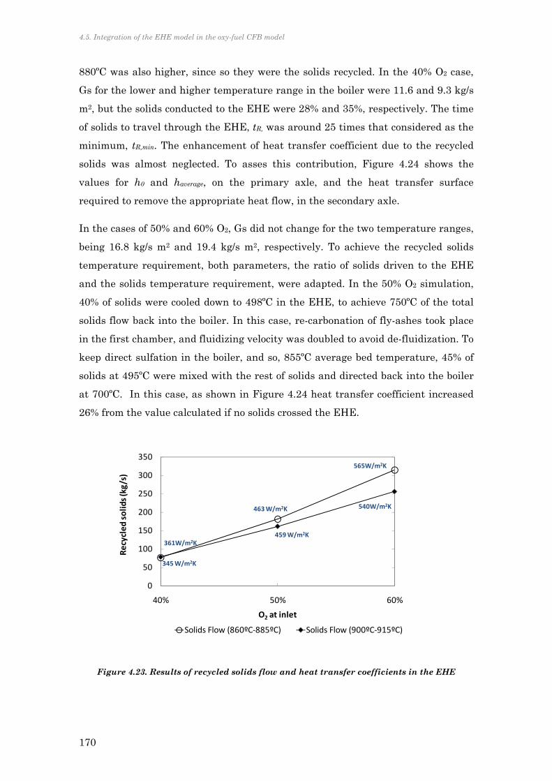
4.5. Integration of the EHE model in the oxy-fuel CFB model
170
880ºC was also higher, since so they were the solids recycled. In the 40% O2 case,
Gs for the lower and higher temperature range in the boiler were 11.6 and 9.3 kg/s
m2, but the solids conducted to the EHE were 28% and 35%, respectively. The time
of solids to travel through the EHE, tR, was around 25 times that considered as the
minimum, tR,min. The enhancement of heat transfer coefficient due to the recycled
solids was almost neglected. To asses this contribution, Figure 4.24 shows the
values for h0 and haverage, on the primary axle, and the heat transfer surface
required to remove the appropriate heat flow, in the secondary axle.
In the cases of 50% and 60% O2, Gs did not change for the two temperature ranges,
being 16.8 kg/s m2 and 19.4 kg/s m2, respectively. To achieve the recycled solids
temperature requirement, both parameters, the ratio of solids driven to the EHE
and the solids temperature requirement, were adapted. In the 50% O2 simulation,
40% of solids were cooled down to 498ºC in the EHE, to achieve 750ºC of the total
solids flow back into the boiler. In this case, re-carbonation of fly-ashes took place
in the first chamber, and fluidizing velocity was doubled to avoid de-fluidization. To
keep direct sulfation in the boiler, and so, 855ºC average bed temperature, 45% of
solids at 495ºC were mixed with the rest of solids and directed back into the boiler
at 700ºC. In this case, as shown in Figure 4.24 heat transfer coefficient increased
26% from the value calculated if no solids crossed the EHE.
Figure 4.23. Results of recycled solids flow and heat transfer coefficients in the EHE
0
50
100
150
200
250
300
350
40% 50% 60%
Recycled solids (kg/s)
O2 at inlet
Solids Flow (860ºC‐885ºC) Solids Flow (900ºC‐915ºC)
361W/m2K459 W/m2K
565W/m2K
345 W/m2K
463 W/m2K 540W/m2K

Chapter 4. The influence of solids recirculation on heat transfer coefficients in an external heat exchanger
171
When inlet gas contained 60% O2, boiler temperature was kept around 905ºC,
reaching indirect sulfation conditions, by cooling 55% of recycled solids down to
442ºC, to reach 700ºC in the total solids recycled flow back into the boiler. This
meant an increase of heat transfer up to 45%, compared to the coefficient for 40%
O2, since tR was then 6 times the tR,min. The first chamber had to increase the
fluidizing velocity up to 1.21 m/s, 2.4 times the design velocity of 0.5 m/s, to avoid
defluidization. To diminish bed temperature down to 860ºC, 67.5% of solids from
the cyclone were cooled down, and so, the total recycled solids back to the boiler
were at 650ºC. In spite of this lower bed temperature, calcination took place for this
conditions and part of the CaO found adequate carbonation conditions in the
second chamber. Fluidizing velocity then was increment 0.86 m/s.
Figure 4.24. Results of heat transfer coefficients with and without recycled solids, and the calculated heat transfer surface required for the proper heat exchange
The required heat transfer surface in air-firing was only 50.3 m2, one fourth of that
needed in 40% O2 case. In these two cases, the heat transfer coefficients got close
values, 351 and 361 W/m2K, respectively. Aiming to use similar boiler geometry for
comparison, solids flow crossing the EHE in the AF case were only 18.8 kg/s,
whereas in the 40% O2 case, they were 76.9 kg/s.
In order to compare the heat transfer coefficients obtained in this work, with those
proposed by other authors, in laboratory, or in the real EHE, Figure 4.25 indicates
0
100
200
300
400
500
600
700
800
0
100
200
300
400
500
600
Air 40% O2 50% O2 60% O2
Req
uired
heat transfer area (m
2)
h(W
/m2K)
O2 at inlet
h (average) h (no solids) Heat transfer area
Average bed temperature 865ºC

4.5. Integration of the EHE model in the oxy-fuel CFB model
172
the values obtained with fully empirical correlations by van Heerden et al. (1953)
or Botterill et al. (1984); the semi-empirical approach for tubes bundle by Kim et al.
(2003) or the expression deduced from the real EHE operation by Man et al. (2012).
They are compared with the values predicted by the present study.
Figure 4.25. Heat transfer coefficients estimated by different authors
The values predicted by this study find within the range of values obtained from
the literature. Only the correlation by Man et al. increases considerably, more than
2.5 times, the value at low O2 concentration. The values obtained by the rest of
expressions, varied only 0.2%-0.7% because the changes on the fluidizing gas
conditions (density, conductivity and viscosity).
At the beginning of this work, it was highlighted the higher heat that would need
to be externally removed in future oxy-fuel fluidized beds. The reason was the
higher fuel power combustion and the lower heat transfer surface available inside
the boiler. The increase of elutriated solids and the lower temperature, at which
these solids will be recycled, allow exchanging more heat in the EHE. Far from
being a drawback, according to the simulations results, the higher values of Gs will
considerably increase the heat transfer coefficients in the EHE. We obtained
increments up to 40% from the case of 40% O2 at inlet to the case of 60% O2 at
0
100
200
300
400
500
600
700
40% 50% 60%
h (W/m
2K)
O2 at inlet
This study Botteril et al. (1984)
Kim et al. (2003) van Heerden et al. (1953)
Man et al. (2012)

Chapter 4. The influence of solids recirculation on heat transfer coefficients in an external heat exchanger
173
inlet. Therefore, heat transfer surfaces would be incremented only moderately to
reach the higher heat removal requirements. On the other hand, however, the heat
transfer surfaces will have to be more carefully located, to take the most advantage
of heat exchange, looking at the increasing un-even distribution of local coefficients
inside the EHE.
4.6 CONCLUSIONS
The EHE heat transfer surfaces of oxy-fuel CFB boilers were quantified for the
first time, by means of a novel correction factor that takes into account the
influence of increasing Gs, applied to a EHE simulation integrated into the overall
CFB boiler model.
With the aim of obtaining the relation between the non-uniformity of heat transfer
in the tubes bundle, and the average heat transfer coefficient in the overall EHE, a
set of experiments was carried out in cold model of EHE. We could observe the
effects of fluid-dynamics on heat transfer coefficients distribution along the EHE. It
was found that the foreseeable increase on solids rate will bring additional
drawbacks related to non-uniform fluidization among the sections of an EHE. In
the experiments, higher cooling rates were observed when increasing gas velocity
and solids flow rate. Up to certain fluidizing velocity, the heat is transferred to the
tubes non-uniformly. At different heights of the tubes, the differences were only
remarkable for the upper tubes row. In order to extrapolate this local heat transfer
coefficients to an average value that can be implemented in a EHE, the obtained
values were averaged.
The average heat transfer coefficient was proved to depend on the residence time of
warm particles in the EHE. Thus, the heat transfer coefficient when no solids are
crossing the EHE is the minimum value. A novel empirical correlation is proposed,
to correct the heat transfer coefficient obtained when no solids are moving
horizontally.
Thanks to this new expression, the heat transfer coefficient when no recycled solids
are present can be modified, for including the enhancing effect of this solids flow.
In order to look at the effect of this increase of heat transfer in a real EHE, a detail
4.6. Conclusions
174
model is developed to be integrated into the overall CFB model previously
explained.
According to the modeling results, it is possible to reduce the heat transfer surface
required for the desired heat exchange, due to the considerable increment heat
transfer coefficients when increasing recycled solids in the oxy-fuel case. Further
attention must be paid to the proper allocation of tubes bundles, to take better
advantage of the trajectory placed by solids traveling along the EHE.

175
CHAPTER 5
SYNTHESIS, CONTRIBUTIONS AND
RECOMMENDATIONS
5.1 SYNTHESIS
In spite of the stabilization of coal demand in developed countries, the role of coal
in the next decades energy mix is still essential. Particularly relevant will be in the
great developing economies, such as India or China, where this fuel is abundant
and avoid external energy dependences. In parallel, the international community
needs to drive its efforts towards politics that commit fossil fuels energetic
companies to drop their CO2 emissions drastically for 2015. In this regard, great
advances have been made towards gaining plant efficiency and therefore, reducing
the tones of CO2 per produced kWh. Still, emissions need a more drastic reduction
if we want to avoid an increment of atmosphere temperature higher than 2ºC.
Here, the CO2 capture and storage (CCS) technologies will have the potential of
reducing up to 25% of CO2 from stationary sources as soon as they will be
commercially available.
Among the CO2 capture technologies, grouping in pre-combustion, post-combustion
and oxy-fuel combustion, this last one is receiving outstanding support by the
national and European authorities. The possibility of implementing oxy-fuel
combustion into circulating fluidized bed technology, contributes to approaching
the concept of “clean-coal technology”. Fluidized bed combustors have the
outstanding feature of offering the possibility of burning a wide variety of fuels
They have the possibility to capture SO2 emissions, adding in-bed limestone. Their
working temperature is lower than in pulverized fuel boilers, which avoids thermal
NOx formation. Additionally to these characteristics, already exploited under air-

5.1 Synthesis
176
firing, applying oxy-fuel combustion technology and being able to capture the CO2
emissions from the coal combustion, or even from blends of coal and other fuels,
makes oxy-fuel combustion in fluidized bed a great opportunity to turn the coal
sustainable in the future power plant designs.
About the implications derived of applying oxy-fuel technology to a conventional
CFB boiler, scarce literature exits, especially when considering high O2
concentrations at inlet. A one dimensional model has been developed. The overall
modeling strategy, in which the model has been based on, is explained in the first
part of Chapter 2. It is based on the already known and validated air-firing semi-
empirical expressions. The model has been divided into three sub-models
interacting with each other: fluid-dynamics, combustion and energy balance of
plant.
For attributing reliability to the developed model, the scarce public experimental
measurements of real air-firing boilers have been compared with the model results.
Additionally, three studies regarding the modeling of large oxy-fuel CFB boilers
have also been used for comparing the model predictions. In spite of having
insufficient information about the published models details, the model developed in
this work fairly fits the predictions in the literature. This has allowed making the
sensibility analysis, trying to draw the main consequences of oxy-fuel deployment
in CFB boilers.
For retrofitting purposes, i.e. with no changes on an air-firing boiler configuration,
the adequate O2 proportion of oxygen at entrance should be around 30%. Higher O2
concentrations lead to smaller cross sectional areas of the boiler. For a given fuel
power required in a boiler, feeding 45% O2 in the comburent, would reduce the
cross sectional area down to 54% of the original one. This involves a reduction of
heat transfer surface along the boiler walls of 23% approximately. The immediate
consequence is the need of resorting to external heat transfer surfaces, i.e.,
external heat exchangers (EHE). This device would need to remove almost 50% of
the total heat of combustion in the case of feeding comburent with 60% O2 content.
The importance of the EHE resides not only in compensating the reduction of heat
transfer surface in the riser, but in managing higher amount of elutriated solids.
The simulations have shown that higher solids densities in the boiler will enhance
heat transfer coefficients to the riser walls. For certain boiler geometry, if

Chapter 5. Synthesis, contributions and recommendations
177
increasing boiler load, higher recycled solids rate will be required. Feeding 60% of
O2 at inlet, fuel input can be increased from 600 to 800 MW if elutriated solids
increase from 25 to 40 kg/m2s. This refers us again to the higher solids crossing the
EHE. An increase of 10% of heat removal will be required in this device for said
changing load.
Applying EHEs to conventional boilers was not essential during air-firing
operation. But for oxy-fuel combustion it was here demonstrated to be crucial for
accomplishing the boiler energy balance. However, several operational and design
uncertainties will need to be solved, before deploying first demonstration oxy-CFB
boiler.
The design of the future EHE will imply two relevant distinguishing features of
oxy-firing operation: the influence of gas composition on the determination of the
heat transfer coefficients and the greater amount of elutriated solids, cooled down
in the EHE. The CIRCE bubbling fluidized bed pilot plant presents the adequate
bubbling working regime to obtain results of heat transfer coefficient for a wide
range of oxy-fuel conditions and extracting further conclusions on possible effects of
gas composition on heat transfer coefficients. The range of O2 concentration at inlet
reached values as high as 60%. Such a high concentration was scarcely achieved in
pilot plants due, in most cases, to the limiting bed cooling capacity. Measurements
of heat transfer coefficients were taken when cooling was needed to control the
combustion temperature. Water could circulate through one or more of the four
cooling jackets, depending on the cooling requirements. Heat transfer coefficients
were indirectly measured by energy balance with the water mass flow and
temperatures. There are no previous results on heat transfer measurements under
oxy-fuel combustion, up to date.
The pilot plant is characterized by two important performance parameters: the
fluidizing velocity and the bed temperature. These two parameters are common for
all the fluidized bed plants working on combustion. Particularly for characterizing
oxy-fuel combustion, the composition of the oxidant gas is the other key parameter
in the plant operation. These three factors have been analyzed and their influence
on heat transfer was examined. The three of them are, however, interrelated. O2
concentration and bed temperature varied the gas density and thus, the fluidizing
velocity. At the same time, the fluidizing velocity will affect the heat transfer
coefficients and consequently, bed temperature would be influenced. For

5.1 Synthesis
178
accounting for this kind of dependences, non-dimensional numbers have been used
for comparison. It was detected no dominant effect of non-dimensional numbers on
the heat transfer. This is mainly offset by the different fluidization velocities in AF
and OF operation. In the former, uf was kept over 1 m/s, whereas OF required
lower velocities, around 0.9 m/s. It was then determined the adequate semi-
empirical correlations for the effective thermal conductivity and the residence time
of particles at the heat transfer surface. Hence, a semi-empirical mechanistic
approach is recommended for a good agreement with the experimental heat
transfer coefficients obtained during oxy-fuel operation. It was demonstrated the
relevance of the gaseous film resistance in the oxy-fuel tests, and a new empirical
coefficient was deduced for both modes. As examined in Chapter 3, section 3.5, the
recommended expressions to predict heat transfer coefficients during oxy-fuel
combustion yield:
filmpacket
br
hh
hh11
1)1(
Where:
1/2
1
cc
cb
bb
bepp,pmfpgg
k
k0.057log0.757logε0.28
g
sg
packet
uδ
d6.52δ
uδ
d0.7δcε1ρudC0.1ρ
k
kk...
h
g
s
...
p
gfilm d
kMh with M=6.51 for oxy-firing and M=11.33 for air-firing
The larger amount of solids arriving at the EHE will influence the values and
distribution of the average and local heat transfer coefficients, respectively. A
review of the difficulties associated with the estimation of heat transfer to the
tubes of a heat exchanger has been examined. By the use of a scaled-down EHE, it
was possible to experimentally confirm the influence of heat transfer coefficients
when horizontal movement of solids took place. The increase of solids rate stressed
the inequalities of the local heat transfer coefficient, whereas the longer residence
time taken by particles to travel through the EHE allows higher average heat
transfer coefficient. The contribution of this parameter to the average heat transfer

Chapter 5. Synthesis, contributions and recommendations
179
coefficient was correlated by means of a new expression, as developed in Chapter 4,
section 4.4:
322073242 .Θ.Η
This expression allows modifying the heat transfer coefficient previously deduced
for stationary conditions, and therefore, accounting for the enhancement of heat
transfer when recirculation of solids takes place.
A real design of an EHE was then simulated and integrated in the existing CFB
model previously developed. This is the first time that such a model is developed to
predict the heat transfer area required in oxy-fuel operation. The EHE sub-model
must fulfill the energy balance requirements previously set for the CFB model. The
temperature, at which solids must be recycled back into the boiler, in order to keep
the desired boiler temperature, is accomplished with this sub-model. The
expressions for the heat transfer coefficient and the enhancement due to recycled
mass flow of solids were included in the EHE sub-model. Hence, it was possible to
determine the increase on the heat transfer surface, for different O2 concentration
in the oxidant stream, and two ranges of boiler temperature required. It was then
recognized that, in spite of doubling the heat transfer surface requirements, when
O2 concentration increased 10%, the heat transfer surface increases less than
expected if solids flow influence were not included in the heat transfer evaluation.
This thesis demonstrates that heat transfer surface design, arrangement and
allocation, will differ in future oxy-fuel CFB boilers. Particularly, the heat transfer
in the EHE will need address the influence of fluidizing gas composition and
recycled solids, for an adequate and efficient heat exchanger configuration.
5.2 CONTRIBUTIONS
This thesis aimed to demonstrate that heat transfer surfaces design in oxy-fuel
CFB boilers will have to be revised and adapted to the new mode of operation.
Thus, the specific contributions are following summarized:
Chapter 2
‐ The contribution of this chapter is the oxy-fuel large-scale CFB model. The
original simulation developed in this chapter has been based on the semi-

5.4. Publications
180
empirical expressions already validated for air-firing combustion. The
estimations drawn from the model have been compared with air-firing CFB
boilers data first, and with three oxy-fuel CFB models available in the
literature.
‐ The heat share of heat removal in the overall CFB loop has been quantified,
for the three parts of the heat balance of the plant: the boiler walls, the
convection pass and the external heat exchanger. The heat transfer shares
have been simulated for different O2 concentrations at inlet and varying the
boiler cross sectional area. It was also run for three different fuel loads,
adapting the secondary air and the fluidizing velocity to the elutriated
solids requirements; and modifying the temperature at which solids are
recycled back into the boiler. The results of this study were published in
Bolea et al. (2012b)
‐ It was here proposed the two key differences between the EHE of an air-
firing and oxy-firing CFB boilers, that will influence heat transfer
coefficient in the future EHEs: the fluidizing gas composition and the
influence of increasing recycled solids rate
Chapter 3
‐ An original theoretical analysis of heat transfer during oxy-fuel in fluidized
beds, was first carried out, considering the different models available in the
literature for the air-firing case and assessing the potential influences of
oxy-fuel combustion predicted by these approaches.
‐ In this chapter the heat transfer coefficients measured during oxy-fuel in
the bubbling fluidized bed combustor in CIRCE are presented. As a relevant
remark, the O2 concentration in the oxidant stream ranged up to 60%. This
high value is uncommonly found in the literature, and it requires a great
cooling flexibility. This is the first time that heat transfer coefficients are
quantified during oxy-fuel operation. Part of this analysis was included in
the book Oxygen-Enhanced Combustion (Baukal Jr., 2013).
‐ The wide range of operational conditions allowed to compare the obtained
heat transfer coefficients with the different non-dimensional numbers that
accounts for the gas composition, gas properties, bed temperature and
fluidizing velocity.

Chapter 5. Synthesis, contributions and recommendations
181
‐ The experimental results during air and oxy-firing operation were further
treated in order to propose an appropriate approach that can predict the
heat transfer coefficients to the walls during oxy-fuel combustion. The
packet renewal model is recommended. The film thermal resistance was
revealed as the differentiate term between air and oxy-firing heat transfer
expressions. The empirical value for the film thermal resistance is proposed
for both, air and oxy-firing modes.
Chapter 4
‐ A theoretically review of the literature on cold models and real EHE
intended forecast the influence of increasing recycled solids on heat
transfer. The existing cold model experiments of EHE did not account for a
drastic increase of the solids flow rate, as it will be expected in EHE of large
oxy-fuel CFB boilers, whereas the available data of real EHE exhibits a
clear influence of Gs on heat transfer coefficients.
‐ A tests campaign was carried out in a cold EHE model, de-attached from the
rest of the cold CFB loop and local heat transfer coefficients were measured
in different tubes location. It was confirmed that uniformity of fluidization
is lost when solids crossing the EHE are increase.
‐ The average heat transfer coefficient was related to the time that particles
take to cross the EHE. Together with data from the literature, a new
correlation to account for this contribution was deduced.
‐ An original EHE simulation was developed, for being integrated on the
overall CFB simulation. The expressions for heat transfer prediction,
previously deduced experimentally were implemented. The risk of EHE de-
fluidization, for different O2 concentration cases was also included in the
EHE sub-model. This allowed quantifying the increments of heat transfer
surfaces that will be needed in future EHE designs. These increments were
moderated by the enhance of heat transfer coefficients, due to the solids
recirculation.

5.3. Recommendations and future work
182
5.3 RECOMMENDATIONS AND FURTHER WORK
This work aims to be an impulse towards the near term deployment of second
generation of oxy-fuel CFB boilers. The large oxy-fuel CFB boiler model here
developed must be the basis to accurately predict the changes in the heat transfer
surfaces inside the boiler itself. To achieve this level of detail, an additional
dimension in the model will be recommendable, also to account for the extended
heat transfer surfaces, so as the hanging wing walls. The lately proposed
combustion model of fuel particles in fluidized beds (Guedea et al., 2013) could be
included to get a more precise allocation of the energy release cells. Additionally,
the attrition phenomena that influence the sulfation reactions (Scala and Salatino,
2010) will have to be integrated into the model, to improving the contribution
estimation of sulfation-calcination reaction into the boiler energy balance, and to
further assess the influence on the re-carbonation reactions in the EHE.
The proper emplacement of heat transfer surfaces in the oxy-fuel CFB boilers and
in their EHE devices will be one of the key issues to optimize the energy penalties
associated to CO2 capture technologies. The maximum efficiency of the boiler will
reside on the proper steam circuit design for the new heat transfer areas
configuration. This will contribute to the overall plant efficiency that would mean
the turning point to allow oxy-fuel becoming commercially feasible. The O2GEN
European Project aims to diminish the overall energy penalty of the oxy-fuel
system to the half of the current state of the art. This will mean a joint effort
between minimizing the electricity consumption by the Air Separations Unit; the
integration of the CO2 compression train with the whole system; and optimizing
the boiler performance, from the basis of the study developed here.
In this work, it has been recognized the uncertainties associated to the appropriate
way of estimating heat transfer coefficients and, additionally, the variation of the
heat transfer coefficient with the location of the tubes, due to non-uniformities of
fluidization in some areas of the EHE. It is urgent to solve this problem, developing
a methodology to properly place the heat transfer tubes in the tubes bundles,
although construction symmetry could be loose. The heat transfer coefficient will be
influenced by the fluidizing gas composition as confirmed in this thesis and further
experiments should be carried out similar to the ones run in CIRCE BFB, but with
finer particle diameter, for resembling the conditions of the EHE. Additionally,
Chapter 5. Synthesis, contributions and recommendations
183
including horizontal immersed surfaces would be desirable, to ascertain the
influence of the change of fluidynamics, affected by changes in the fluidizing gas
composition.
Regarding the potential problems involved with the EHE device, when fluidized
with RFG, it will be an essential issue to account for the potential corrosion
problems derived from the presence of corrosive or acid substances in the fluidizing
gas. This will lead to material corrosion issues and also to fouling of products of
reactions with the bed material and elutriated solids. To acquire feasible results,
experimentation must be carried out in oxy-fuel combustion with flue gas
desulfurization, since the pollutant content in the diluting stream, will actively
participate in the deposition and fouling, so as in the acid corrosion reactions.
5.4 PUBLICATIONS
The diffusion of some of the results was carried out by means of publication in
papers in journals and conferences. The publications related to the performance of
the present thesis are presented, from the results from the CFB modeling, to the
results from the experiments carried out in the oxy-fuel fluidized bed pilot plant.
Afterwards, they are also indicated some publications not related to oxy-fuel
combustion, but with CO2 capture and power plant integration.
International journal articles:
1. Bolea, I., L. M. Romeo and D. Pallarés (2012). The role of external heat
exchangers in oxy-fuel circulating fluidized bed. Applied Energy 94(0): 215-
223.
In this paper a large scale oxy-fuel circulating fluidized bed boiler has been
modeled, in collaboration with Chalmers University. The main results of the
sensitivity analysis were explained. This article is based on the Chapter 2 of
the current thesis
2. Romeo, L. M., L. I. Díez, I. Guedea, I. Bolea, C. Lupiáñez, A. González, J.
Pallarés and E. Teruel (2011). Design and operation assessment of an
oxyfuel fluidized bed combustor. Experimental Thermal and Fluid Science
35(3): 477-484.
In this paper the work carried out for the design and the operation of the
oxy-fuel pilot plant, carried out by the whole oxy-fuel research team is

5.4 Publications
184
explained. Results of the oxy-fuel combustion of biomass and coal blends are
shown. Section 3.3.2 is included in this article.
3. Font, O., P. Córdoba, C. Leiva, L. M. Romeo, I. Bolea, I. Guedea, N. Moreno,
X. Querol, C. Fernandez and L. I. Díez (2012). Fate and abatement of
mercury and other trace elements in a coal fluidised bed oxy combustion pilot
plant. Fuel 95(0): 272-281
In this article, the longest oxy-fuel tests were needed for the feasible
samples gathering of ashes in the bed, cyclone and bag filter. Main trace
elements, including mercury, were measured in collaboration with Institute
of Environmental Assessment and Water Research (IDÆA-CSIC). Part of
the measurements of heat transfer coefficients were obtained during the
tests explained here.
4. Ordorica-Garcia, G., M. Carbo, I. Bolea and M. Nikoo (2012). Technology
Options and Integration Concepts for Implementing CO2 Capture in Oil
Sands Operations. Journal of Canadian Petroleum Technology 51(5): 362-
375.
This was a joint collaboration between institutions from Canada, The
Netherlands and Spain, aiming to look for the most suitable CO2 capture
technology integrated in any of the phases of the oil sands operations. The
oxy-fuel state of the art in this paper is based on the Chapter 1 of this
thesis.
5. Lupiáñez, C., I. Guedea, I. Bolea, L. I. Díez, and L. M. Romeo, (2013).
"Experimental study of SO2 and NOx emissions in fluidized bed oxy-fuel
combustion." Fuel Processing Technology 106(0): 587-594.
This article analyzed the SO2 and NOx emissions during air and oxy-firing
modes, for two different types of coal and blends of them. Several tests
explained in this paper, were also used for the heat transfer measurements
During the last years, in parallel to the research carried out for the development of
this thesis, the following papers were also published in international journals,
related to the integration of CO2 capture technologies in the overall power plant
process:
6. Romeo, L. M., I. Bolea and J. M. Escosa (2008). Integration of power plant
and amine scrubbing to reduce CO2 capture costs. Applied Thermal
Engineering 28(8–9): 1039-1046.

Chapter 5. Synthesis, contributions and recommendations
185
7. Romeo, L. M., S. Espatolero and I. Bolea (2008). Designing a supercritical
steam cycle to integrate the energy requirements of CO2 amine scrubbing.
International Journal of Greenhouse Gas Control 2(4): 563-570.
8. Romeo, L. M., I. Bolea, Y. Lara and J. M. Escosa (2009). Optimization of
intercooling compression in CO2 capture systems. Applied Thermal
Engineering 29(8–9): 1744-1751.
9. Bolea, I., J. Uche and L. M. Romeo (2009). Integration of MED with
captured CO2 flue gas compression. Desalination and Water Treatment 7(1-
3): 124-131.
10. Sanpasertparnich, T., R. Idem, I. Bolea, D. de Montigny and P.
Tontiwachwuthikul (2010). Integration of post-combustion capture and
storage into a pulverized coal-fired power plant. International Journal of
Greenhouse Gas Control 4(3): 499-510
Conference proceedings involving oxy-fuel in fluidized bed:
A. Romeo, L. M., I. Guedea, I. Bolea, A. González, C. Lupiáñez, J. Pallares and
L. I. Diez (2009). First Results in an Oxyfuel Combustion Fluidized Bed. 1st
Oxyfuel Combustion Conference. Cottbus, Germany.
B. Guedea, I., I. Bolea, C. Lupiáñez, N. Cortés, E. Teruel, J. Pallarés, L. I.
Díez and L. M. Romeo (2011). Control system for an oxy-fuel combustion
fluidized bed with flue gas recirculation. Energy Procedia 4(0): 972-979.
C. Lupiáñez, C., I. Guedea, I. Bolea, J. Pallarés, L. I. Díez and L. M. Romeo
(2011). Oxy-firing of high sulphur coal in CIRCE fluidized bed pilot plant.
5th International Conference on Clean Coal Technologies. Zaragoza, Spain.
D. Font, O., P. Córdoba, C. Leiva, L. M. Romeo, I. Bolea, I. Guedea, N.
Moreno, X. Querol, C. Fernandez-Pereira and L. I. Díez (2011). Speciation
and fate of mercury in oxy coal combustion. International Conference on
Coal Science and Technology Oviedo, Spain.
E. Bolea, I., C. Lupiáñez, I. Guedea, L. M. Romeo and L. I. Díez (2012). Direct
Sulfation in oxy-fuel fluidzied bed boilers. 21st International Conference on
Fluidized Bed Combustion, Naples, Italy.

5.4 Publications
186
Book contributions:
A. Romeo, L. M., L. I. Díez, P. Lisbona, A. González, I. Guedea, C. Lupiáñez, A.
Martínez, Y. Lara and I. Bolea (2010). Captura y almacenamiento de CO2.
Zaragoza, Prensas Universitarias de Zaragoza.
B. Jia, L., Romeo, L. M., Díez, L. I., Guedea, I., Bolea, I. and Lupiañez, C.
(2013). Oxy-fuel Fluidized Bed Combustion. In Oxygen-Enhanced
Combustion, CRC Press. Taylor and Fracis: 649-674.

187
REFERENCES
Abdulally, I. F. and Randolph, N. J. (1989). Fluidized Bed Steam Generation
System And Method having an External Heat Exchanger. Patent, U. S., Foster
Wheeler Energy Corporation.
Adánez, J. and Diego, L. F. d. (1995). Modeling of Carbon Combustion Efficiency in
Circulating Fluidized Bed Combustors. 1. Selection of Submodels and Sensitivity
Analysis. Industrial & Engineering Chemistry Research 34(9): 3129-3138.
Adanez, J., Gayán, P., Grasa, G., de Diego, L. F., Armesto, L. and Cabanillas, A.
(2001). Circulating fluidized bed combustion in the turbulent regime: modelling of
carbon combustion efficiency and sulphur retention. Fuel 80(10): 1405-1414.
Aibéo, A. and Pinho, C. (2003). Heat transfer Modelling in a Circulating Fluidised
Bed Biomass Boiler. International Conference of Renewable Energies and Power
Quality. Vigo, Spain.
Al-Busoul, M. A. and Abu-Ein, S. K. (2003). Local heat transfer coefficients around
a horizontal heated tube immersed in a gas fluidized bed. Heat and Mass Transfer
39(4): 355-358.
Alagöz, E. (2006). Mathematical modeling of fluidized bed combustors with
radiation model, Middel East Technical University. Master of Science.
Alvarez, I., Muñoz, F., Lupion, M., Otero, P., Hotta, A., Kuivalainen, R. and
Alvarez, J. (2011). CIUDEN CFB boiler technological development. 2nd Oxyfuel
Combustion Conference. Queensland, Australia
Andersson, B.-Å. (1988). Heat transfer in stationary fluidized bed boilers. PhD
Thesis. Chalmers University of Technology.
Andersson, B.-Å. and Leckner, B. (1992). Experimental methods of estimating heat
transfer in circulating fluidized bed boilers. International Journal of Heat and
Mass Transfer 35(12): 3353-3362.

References
188
Andersson, B. Å. (1996). Effects of bed particle size on heat transfer in circulating
fluidized bed boilers. Powder Technology 87(3): 239-248.
Andersson, K. and Johnsson, F. (2006). Flame and radiation characteristics of gas-
fired O2/CO2 combustion. Fuel 86(5-6): 656-668.
Anheden, M., Yan, J. and De Smedt, G. (2005). Denitrogenation (or Oxyfuel
Concepts). Oil & Gas Science and Technology 60(3): 485-495.
Arena, U., Chirone, R., D'Amore, M., Miccio, M. and Salatino, P. (1995). Some
issues in modelling bubbling and circulating fluidized-bed coal combustors. Powder
Technology 82(3): 301-316.
Barbucci, P. (2009). CO2 Capture and Storage- An utility view. 3rd International
Symposium on Capture and geological storage of CO2, Paris, France.
Baskakov, A. P. (1964). The mechanism of heat transfer between a fluidized bed and
a surface. International Chemical Engineering 4(2): 320-323.
Baskakov, A. P. and Leckner, B. (1997). Radiative heat transfer in circulating
fluidized bed furnaces. Powder Technology 90(3): 213-218.
Basu, P. (1999). Combustion of coal in circulating fluidized-bed boilers: a review.
Chemical Engineering Science 54(22): 5547-5557.
Basu, P. (2006). Combustion and gasification in fluidized beds, Taylor & Francis.
Basu, P. and Nag, P. K. (1996). Heat transfer to walls of a circulating fluidized-bed
furnace. Chemical Engineering Science 51(1): 1-26.
Baukal, C. E. (2000). Heat transfer in industrial combusiton, CRC Press LLC.
Baukal Jr., C. E. (2013). Oxygen-Enhanced Combustion, CRC Press. Taylor and
Fracis.
Becher, V. (2008). Controlled Staging with Non-Stoichiometric Burners for Oxyfuel
Processes-Experimental Validation. 2nd Young Researchers Forum on Oxyfuel
Combustion, Gotheborg, Sweden.
Bolea, I., Lupiáñez, C., Guedea, I., Romeo, L. M. and Díez, L. I. (2012a). Direct
Sulfation in oxy-fuel fluidzied bed boilers. 21st International Conference on
Fluidized Bed Combustion, Naples, Italy.

References
189
Bolea, I., Romeo, L. M. and Pallarés, D. (2012b). The role of external heat
exchangers in oxy-fuel circulating fluidized bed. Applied Energy 94(0): 215-223.
Botterill, J. S. M. (1989). Fluidized Bed Heat Transfer. Combustión en Lechos
Fluidizados. COMETT, CEE, Zaragoza, Spain.
Botterill, J. S. M., Teoman, Y. and Yüregir, K. R. (1984). Factors affecting heat
transfer between gas-fluidized beds and immersed surfaces. Powder Technology
39(2): 177-189.
BP (2011a). BP Energy Outlook 2030.
BP (2011b). BP Statistical Review of World Energy.
Breitholtz, C. and Leckner, B. (1997). Heat balance over the fluid-dynamic
boundary layer of a circulating fluidized bed furnace. International Journal of Heat
and Mass Transfer 41(8-9): 1013-1024.
Breitholtz, C., Leckner, B. and Baskakov, A. P. (2001). Wall average heat transfer
in CFB boilers. Powder Technology 120(1-2): 41-48.
Breitholtz., C. and B., L. (2000). Translation of heat transfer measurements from
laboratory CFBs to the conditions of CFB-boilers. IV Minsk International Forum on
Heat and Mass Transfer, Minsk, Belarus.
Buhre, B. J. P., Elliott, L. K., Sheng, C. D., Gupta, R. P. and Wall, T. F. (2005).
Oxy-fuel combustion technology for coal-fired power generation. Progress in Energy
and Combustion Science 31(4): 283-307.
Burchhardt, U. (2009). Experiences from Commissioning and Test Operation of
Vattenfall's Oxyfuel Pilot Plant. 1st Oxyfuel Combustion Conference, Cottbus,
Germany.
Burnard, H. and Bhattacharya, S. (2011). Power Generation from Coal. Ongoing
Developments and Outlook, International Energy Angency.
Coleman, H. W. and Steele, W. G. (1999). Experimentation and Uncertanity
Analysis for Engineers, John Wiley & Sons, Inc.
Croiset, E. and Thambimuthu, K. V. (2001). NOx and SO2 emissions from O2/CO2
recycle coal combustion. Fuel 80(14): 2117-2121.

References
190
Czakiert, T. (2011). Personal communication.
Czakiert, T., Bis, Z., Muskala, W. and Nowak, W. (2006). Fuel conversion from oxy-
fuel combustion in a circulating fluidized bed. Fuel Processing Technology 87(6):
531-538.
Czakiert, T., Sztekler, K., Karski, S., Markiewicz, D. and Nowak, W. (2010). Oxy-
fuel circulating fluidized bed combustion in a small pilot-scale test rig. Fuel
Processing Technology 91(11): 1617-1623.
Chen, J. C. (2003). Surface Contact---Its Significance for Multiphase Heat Transfer:
Diverse Examples. Journal of Heat Transfer. Max Jakob award lecture 125(4): 549-
566.
Chen, J. C., Grace, J. R. and Golriz, M. R. (2005). Heat transfer in fluidized beds:
design methods. Powder Technology 150(2): 123-132.
Chen, T.-P. and Saxena, S. C. (1977). Mathematical modelling of coal combustion in
fluidized beds with sulphur emission control by limestone or dolomite. Fuel 65: 401-
413.
Chen, Y. and Xiaolong, G. (2006). Dynamic modeling and simulation of a 410 t/h
Pyroflow CFB boiler. Computers & Chemical Engineering 31(1): 21-31.
Cheng, L., Wang, Q., Shi, Z., Luo, Z., Ni, M. and Cen, K. (2007). Heat transfer in a
large-scale circulating fluidized bed boiler. Energy Power Eng. China 1(4): 477–
482.
Daki, D., Honing, G. v. d. and Valk, M. (1989). Fragmentation and swelling of
various coals during devolatilization in a fluidized bed. Fuel 68: 911-916.
Davidson, J. F. (2000). Circulating fluidised bed hydrodynamics. Powder
Technology 113(3): 249-260.
Davidson, J. F., Clift, R. and Harrison, D. (1985). Fluidization. London, Academic
Press Inc.
de Diego, L. F., de las Obras-Loscertales, M., García-Labiano, F., Rufas, A., Abad,
A., Gayán, P. and Adánez, J. (2011). Characterization of a limestone in a batch
fluidized bed reactor for sulfur retention under oxy-fuel operating conditions.
International Journal of Greenhouse Gas Control 5(5): 1190-1198.

References
191
de Diego, L. F., Rufas, A., García-Labiano, F., de las Obras-Loscertales, M., Abad,
A., Gayán, P. and Adánez, J. (2012). Optimum temperature for sulphur retention in
fluidised beds working under oxy-fuel combustion conditions. In press. Fuel(0).
de Souza-Santos, M. L. (2007). A new version of CSFB, comprehensive simulator for
fluidised bed equipment. Fuel 86(12-13): 1684-1709.
Decker, N. and Glicksman, L. R. (1983). Heat transfer in large particle fluidized
beds. International Journal of Heat and Mass Transfer 26(9): 1307-1320.
Di Natale, F., Lancia, A. and Nigro, R. (2008). A single particle model for surface-to-
bed heat transfer in fluidized beds. Powder Technology 187(1): 68-78.
Diego, L. F. d., Londonot, C. A., Wang, X. S. and Gibbs, B. M. (1996). Influence of
operating parameters on NOx and N20 axial profiles in a circulating fluidized bed
combustor. Fuel 75(8): 971-978.
Dow, W. M. and Jakob, M. (1951). Heat transfer between a verticl tube and a
fluidized air-solid flow. Chemical Engineering Progress 58: 637-648.
Duan, L., Zhao, C., Zhou, W., Qu, C. and Chen, X. (2011a). Effects of operation
parameters on NO emission in an oxy-fired CFB combustor. Fuel Processing
Technology 92(3): 379-384.
Duan, L., Zhao, C., Zhou, W., Qu, C. and Chen, X. (2011b). O2/CO2 coal
combustion characteristics in a 50 kWth circulating fluidized bed. International
Journal of Greenhouse Gas Control 5(4): 770-776.
Eddings, E. G., Okerlund, R. and Bool, L. E. (2009). Pilot-scale evaluation of
oxycoal firing in circulating fluidized bed and pulverized coal-fired test facilities.
1st Oxyfuel Combustion Conference. Cottbus, Germany.
EIA (2011). International Energy Outlook 2011. U.S. Energy Information
Administration.
Ergun, S. and Orning, A. A. (1949). Flow through randomly packed columns and
fluidized beds. Fluid Industrial & Engineering Chemistry 41: 1179–1184.
Eriksson, M. and Golriz, M. R. (2005). Radiation heat transfer in circulating
fluidized bed combustors. International Journal of Thermal Sciences 44(4): 399-
409.

References
192
ExxonMobil (2012). 2012 The Outlook for Energy: A view to 2040.
García-Labiano, F., Abad, L. F., de Diego, L. F., Gayán, P. and Adánez, J. (2002).
Calcination of calcium-based sorbents at pressure in a broad range of CO2
concentrations. Chemical Engineering Science 57: 2381-2393.
García-Labiano, F., Rufas, A., de Diego, L. F., Obras-Loscertales, M. d. l., Gayán,
P., Abad, A. and Adánez, J. (2011). Calcium-based sorbents behaviour during
sulphation at oxy-fuel fluidised bed combustion conditions. Fuel 90(10): 3100-3108.
Gayan, P., Adanez, J., de Diego, L. F., García-Labiano, F., Cabanillas, A., Bahillo,
A., Aho, M. and Veijonen, K. (2004). Circulating fluidised bed co-combustion of coal
and biomass. Fuel 83(3): 277-286.
Glicksman, L. R. (2007). Radiation Heat Transfer in Circulating Fluidized Beds.
The 12th International Conference on Fluidization - New Horizons in Fluidization
Engineering, Vancouver, Canada.
Glicksman, L. R. and Decker, N. (1982). Heat transfer from an immersed surface to
adjacent particles in a fluidized bed; the role of radiation and particle packing. 7th
International Heat Transfer Conference, München, Germany.
Grace, J. R., Avidan, A. A. and Knowlton, T. M. (1997). Circulating fluidized beds,
Blackie Academic and Professional.
Grewal, N. S. (1981). A Generalized Correlation for Heat Transfer Between a Gas-
Solid Fluidized Bed of Small Particles and an Immersed Staggered Array of
Horizontal Tubes. Powder Technology 30: 145-154.
Grewal, N. S. and Saxena, S. C. (1981). Maximum heat transfer coefficient between
a horizontal tube and a gas-solid fluidized bed. Industrial & Engineering
Chemistry Process Design and Development 20(1): 108-116.
Guedea, I., Díez, L. I., Pallarés, J. and Romeo, L. M. (2011). Influence of O2/CO2
mixtures on the fluid-dynamics of an oxy-fired fluidized bed reactor. Chemical
Engineering Journal 178(0): 129-137.
Guedea, I., Pallarès, D., Díez, L. I. and Johnsson, F. (2013). Conversion of large coal
particles under O2/N2 and O2/CO2 atmospheres - Experiments and modeling.
Fuel Processing Technology 112: 118-128.

References
193
Gungor, A. (2009). One dimensional numerical simulation of small scale CFB
combustors. Energy Conversion and Management 50(3): 711-722.
Gungor, A. and Eskin, N. (2008). Two-dimensional coal combustion modeling of
CFB. International Journal of Thermal Sciences 47(2): 157-174.
Hack, H. and Shah, M. (2008). Oxy-fuel Coal-Fired Combustion Power Plant
System Integration. 3rd International Oxy-Combustion Network Meeting,
Yokohama, Japan.
Hamidipour, M., Mostoufi, N., Sotudeh-Gharebagh, R. and Chaouki, J. (2005).
Experimental investigation of particle contact time at the wall of gas fluidized beds.
Chemical Engineering Science 60(15): 4349-4357.
Hannaes, J., Renz, U. and van den Bleek, C. M. (1995). The IEA model for
circulating fluidized bed combustion. 3th International Conference on Fluidized
Bed Combustion. Henschel, K. J. 1: 287-296.
Harris, A. T., Thorpe, R. B. and Davidson, J. F. (2002). Characterisation of the
annular lm thickness in circulating fluidised-bed risers. Chemical Engineering
Science 57: 2579-2587.
Hartge, E.-U., Klett, C. and Werther, J. (2007). Dynamic simulation of the particle
size distribution in a circulating fluidized bed combustor. Chemical Engineering
Science 62(1-2): 281-293.
Hayhurst, A. N. and Lawrence, A. D. (1996). The Amounts of NO, and N,O Formed
in a Fluidized Bed Combustor during the Burning of Coal Volatiles and Also of
Char. Combustion and Flame 105: 341-357.
Heikkinen, M., Hiltunen, T., Liukkonen, M., Kettunen, A., Kuivalainen, R. and
Hiltunen, Y. (2009). A modelling and optimization system for fluidized bed power
plants. Expert Systems with Applications 36(7): 10274-10279.
Horio, M. (1997). Hydrodynamics. Circulating Fluidized Beds. Blackie Academic
and Professional.
Howard, J. R. (1989). Fluidized Bed Technology: principles and applications, Taylor
& Francis.
References
194
Hu, G., Dam-Johansen, K., Wedel, S. and Peter Hansen, J. (2006). Review of the
direct sulfation reaction of limestone. Progress in Energy and Combustion Science
32(4): 386-407.
Huilin, L., Guangbo, Z., Rushan, B., Yongjin, C. and Gidaspow, D. (2000). A coal
combustion model for circulating fluidized bed boilers. Fuel 79(2): 165-172.
Hyytiäinen, I., Mahlamäki, A., Palonen, M., Varonen, M. and Lemmetyinen, H.
(2011). Study of recarbonation in circulating fluidized bed combustion. 10th
International Conference on Circulating Fluidized Beds and Fluidization
Technology. Rusnrive, Oregon, USA.
IEA (2010a). Energy Technology Perspectives. Scenarios and Strategies to 2050.
Executive Summary.
IEA (2010b). Power generation from coal. Measuring and reporting efficiency
Performance and CO2 emissions.
IEA (2011a). CO2 emissions from fuel combustion. Hihlights.
IEA (2011b). World Energy Outlook 2011.
IEA (2011c). World Energy Outlook 2011. Resumen Ejecutivo.
IPCC (2005). Special Report Carbon Dioxide Capture and Storage.
IPCC (2007). Fourth Assessment Report: Climate Change
IPCC (2010). Understanding Climate Change. 22 years of IPCC assessment.
Jäntti, T., Eriksson, T., Hotta, A., Hyppänen, T. and Nuortimo, K. (2007). CFB
Technology- Toward Zero CO2 Emissions. Varkaus, Finland.
Jia, L., Tan, Y. and Anthony, E. J. (2010). Emissions of SO2 and NOx during Oxy-
Fuel CFB Combustion Tests in a Mini-Circulating Fluidized Bed Combustion
Reactor. Energy Fuels 24(2): 910-915.
Jia, L., Tan, Y., Wang, C. and E.J., A. (2007). Experimental Study of Oxy-Fuel
Combustion and Sulfur Capture in a Mini-CFBC. Energy & Fuels 21: 3160-3164.

References
195
Johansson, A., Johnsson, F. and Andersson, B.-A. (2006). The Performance of a
Loop Seal in a CFB Boiler. Journal of Energy Resources Technology 128(2): 135-
142.
Johansson, A., Johnsson, F. and Leckner, B. (2007). Solids back-mixing in CFB
boilers. Chemical Engineering Science 62(1-2): 561-573.
Johnsson, F. (2010). Oxyfuel CFB Combustion – discussion on challenges for
development. 60th IEA-FBC Meeting Göteborg, Sweden.
Johnsson, F. and Leckner, B. (1995). Vertical distribution of solids in a CFB-
furnace 13th International Conference on Fluidized Bed Combustion. Orlando,
Florida, USA.
Jordal, K., Anheden, M., Yan, J. and Strömberg, L. (2004). Oxyfuel combustion for
coal-fired power generation with CO2 capture- Opportunities and challenges 7th
Internationa Conference on Greenhouse Gas Technologies, Vancouver, Canada.
Kather, A. (2007). Oxy-fuel Process for Hard Coal with CO2 Capture. A part of the
ADECOS Project. 2nd Workshop of the International Oxy-Combustion Research
Network., Windsor CT, USA.
Kiga, T., Takano, S., Kimura, N., Omata, K., Okawa, M., Mori, T. and Kato, M.
(1997). Characteristics of pulverized-coal combustion in the system of
oxygen/recycled flue gas combustion. Energy Conversion and Management
38(Supplement 1): S129-S134.
Kim, S. W., Ahn, J. Y., Kim, S. D. and Hyun Lee, D. (2003). Heat transfer and
bubble characteristics in a fluidized bed with immersed horizontal tube bundle.
International Journal of Heat and Mass Transfer 46(3): 399-409.
Kim, S. W., Namkung, W. and Kim, S. D. (2001). Solid Recycle Characteristics of
Loop-seals in a Circulating Fluidized Bed. Chemical Engineering Technology 24(8):
843-849.
Kohl, A. L. and Nielsen, R. D. (1997). Gas Purification, Gulf Professional
Publishing.

References
196
Koornneef, J., Junginger, M. and Faaij, A. (2007). Development of fluidized bed
combustion--An overview of trends, performance and cost. Progress in Energy and
Combustion Science 33(1): 19-55.
Krzywanski, J., Czakiert, T., Muskala, W., Sekret, R. and Nowak, W. (2010a).
Modeling of solid fuel combustion in oxygen-enriched atmosphere in circulating
fluidized bed boiler: Part 2. Numerical simulations of heat transfer and gaseous
pollutant emissions associated with coal combustion in O2/CO2 and O2/N2
atmospheres enriched with oxygen under circulating fluidized bed conditions. Fuel
Processing Technology 91(3): 364-368.
Krzywanski, J., Czakiert, T., Muskala, W., Sekret, R. and Nowak, W. (2010b).
Modeling of solid fuels combustion in oxygen-enriched atmosphere in circulating
fluidized bed boiler: Part 1. The mathematical model of fuel combustion in oxygen-
enriched CFB environment. Fuel Processing Technology 91(3): 290-295.
Kunii, D. and Levenspiel, O. (1991). Fluidization Engineering, Blutterworth-
Heinemann.
Kurosaki, Y., Satoh, I. and Ishize, T. (1995). Mechanisms of Heat Transfer
Enhancement of Gas-Solid Fluidized Bed: Estimation of Direct Contact Heat
Exchange From Heat Transfer Surface to Fluidized Particles Using an Optical
Visualization Technique. Journal of Heat Transfer 117(1): 104-112.
Kyungtae, P., Ikhyun, K., Namjin, J., Moongoo, J., Yukyung, L. and En Sup, Y.
(2011). Cost of energy analysis of integrated gasification combined cycle (IGCC)
power plant with respect to CO2 capture ratio under climate change scenarios.
Advanced Control of Industrial Processes (ADCONIP), 2011 International
Symposium on.
Leckner, B. (1997). Fluidized bed combustion: Mixing and pollutant limitation.
Progress in Energy and Combustion Science 24: 31-61.
Lee, D. K., Noh, D. S., Choi, K. B., Seo, D. M., Ko, C. B. and Lee, E. K. (2009).
Development of 0.1MW class Oxy-PC Swirl Burner with Primary O2 Direct-
injection. 1st Oxyfuel Combustion Conference, Cottbus, Germany.

References
197
Lee, J.-M. and Kim, J.-S. (1999). Simulation of the 200 MWe Tonghae thermal
power plant circulating fluidized bed combustor by using IEA-CFBC model. Korean
Journal of Chemical Engineering 16(5): 640-645.
Levenspiel, O. and Walton, J. S. (1954). Bed wall heat transfer in fluidized systems.
Chemical Engineering Progress Symposium Series 50(9): 1-9.
Lindsay, A. L. and Bromley, L. A. (1950). Thermal Conductivity of Gas Mixtures.
Industrial & Engineering Chemistry 42(8): 1508-1511.
Liu, H., Katagiri, S., Kaneko, U. and Okazaki, K. (2000). Sulfation behavior of
limestone under high CO2 concentration in O2/CO2 coal combustion. Fuel 79: 945-
953.
Lu, J., Lu, X., Liu, H., Wang, H. and He, H. (2010). Calculation and analysis of
dissipation heat loss in large-scale circulating fluidized bed boilers. Applied
Thermal Engineering 30(13): 1839-1844.
Lu, J. D., Flamant, G. and Snabre, P. (1993). Towards a generalized model for
vertical walls to gas--solid fluidized beds heat transfer--I. Particle convection and
gas convection. Chemical Engineering Science 48(13): 2479-2492.
Luan, W., Bowen, B. D., Lim, C. J., Brereton, C. M. H. and Grace, J. R. (2000).
Suspension-to-membrane-wall heat transfer in a circulating fluidized bed
combustor. International Journal of Heat and Mass Transfer 43(7): 1173-1185.
Luan, W., Lim, C. J., Brereton, C. M. H., Bowen, B. D. and Grace, J. R. (1999).
Experimental and theoretical study of total and radiative heat transfer in
circulating fluidized beds. Chemical Engineering Science 54(17): 3749-3764.
Lupiáñez, C., Guedea, I., Bolea, I., Díez, L. I. and Romeo, L. M. (2012).
Experimental study of SO2 and NOx emissions in fluidized bed oxy-fuel
combustion. Fuel Processing Technology(0).
Lupiáñez, C., Guedea, I., Bolea, I., Pallarés, J., Díez, L. I. and Romeo, L. M. (2011).
Oxy-firing of high sulphur coal in CIRCE fluidized bed pilot plant. 5th
International Conference on Clean Coal Technologies. Zaragoza, Spain.
References
198
Man, Z., Haibo, W., Qinggang, L., Yunkai, S. and Guoliang, S. (2012). Heat transfer
characteristics of fluidized bed heat exchanger in a 300 MW CFB boiler. Powder
Technology 222(0): 1-7.
Masoumifard, N., Mostoufi, N., Hamidi, A.-A. and Sotudeh-Gharebagh, R. (2008).
Investigation of heat transfer between a horizontal tube and gas–solid fluidized bed.
International Journal of Heat and Mass Transfer 29: 1504-1511.
Mathur, A., Saxena, S. C. and Chao, A. (1986). Heat transfer from an immersed
vertical tube in a gas-fluidzied bed. Industrial & Engineering Chemistry
Fundamentals 25(1): 156-163.
Mattisson, T. A. and Lyngfelt , A. (1999). The reaction between limestone and SO2
under periodically changing oxidizing and reducing conditions – effect of
temperature and limestone type. Termochimica Acta 325: 59-67.
McCauley, K. J., Farzan, H., Alexander, K. C., McDonald, D. K., Varagani, R.,
Prabhakar, R., Tranier, J.-P. and Perrin, N. (2008). Commercialization of Oxy-Coal
Combustion: Applying Results of a Large 30 MWth Pilot Project. 9th International
Conference on Greenhouse Gas Control Technologies, Washington, D.C., U.S.A.
Mickley, H. S. and Fairbanks, D. F. (1955). Mechanism of heat transfer to fluidized
beds. AIChE Journal 1(3): 374-384.
Mills, A. F. (1995). Transferencia de calor, Irwin.
Molerus, O., Burschka, A. and Dietz, S. (1995a). Particle migration at solid surfaces
and heat transfer in bubbling fluidized beds--I. Particle migration measurement
systems. Chemical Engineering Science 50(5): 871-877.
Molerus, O., Burschka, A. and Dietz, S. (1995b). Particle Migration at solid
surfaces and heat transfer in bubbling fluidized beds- II. Prediction of heat transfer
in bubbling fluidized beds. Chemical Engineering Science 50(5): 879-885.
Myöhänen, K., Eriksson, T., Kuivalainen, R. and Hyppänen, T. (2012). Design and
modelling of a 330 MWe Flex-Burn CFB for oxygen-fired and air-fired combustion.
21st International Conference on fluidized bed combustion, Naples, Italy.
Nsakala, N., Liljedahl, G. N. and Turek, D. G. (2004). Greenhouse gas emissions
control by oxygen firing in Circulating Fluidized Bed Boilers. Phase II-Pilot scale

References
199
testing and updated performance and economics for oxygen fired CFB with CO2
capture. Final Technical Progress Report, ALSTOM Power Inc.
Ochs, T., Oryshchyn, D., Woodside, R., Summers, C., Patrick, B., Gross, D.,
Schoenfield, M., Weber, T. and O'Brien, D. (2009a). Results of initial operation of
the Jupiter Oxygen Corporation oxy- fuel 15 MWth burner test facility. Energy
Procedia 1(1): 511-518.
Ochs, T., Patrick, B., O’Brien, D., Oryshchyn, D., Summers, C., Gerdemann, S.,
Woodside, R., Carney, C., Schoenfield, M. and Turner, P. (2009b). Oxy-Natural Gas
Firing of the Jupiter Oxygen Oxy-Fuel Test Facility. 34th International Technical
Conference on Coal Utilization & Fuel Systems, Clearwater, Florida, USA.
Oka, S. N. (2003). Fluidized Bed Combustion, Marcel Dekker Inc.
Okazaki, K. and Ando, T. (1997). NOx reduction mechanism in coal combustion
with recycled CO2. Energy 22(2-3): 207-215.
Ozawa, M., Umekawa, H., Matsuda, T., Takenaka, N. and Matsubayashi, M.
(1998). Flow Pattern and Heat Transfer in Tube Banks of a Simulated FLuidized
Bed Heat Exchanger. JSME International Journal 41(3): 720-726.
Pallarès, D. and Johnsson, F. (2006). Macroscopic modelling of fluid dynamics in
large-scale circulating fluidized beds. Progress in Energy and Combustion Science
32(5-6): 539-569.
Park, C. K. and Basu, P. (1997). A model for prediction of transient response to the
change of fuel feed rate to a circulating fluidized bed boiler furnace. Chemical
Engineering Science 52(20): 3499-3509.
Patil, D. J., Smit, J., Van Sint Annaland, M. and Kuipers, J. A. M. (2006). Wall-to-
bed heat transfer in gas-solid bubbling fluidized beds. AIChE Journal 52(1): 58-74.
Peña, J. A. P. (2011). Bubbling Fluidized Bed (BFB), when to use this technology?
Industrial Fluidization South Africa. Jojannesburg, South Africa.
Pidwerbecki, D. and Welty, J. R. (1995). Heat transfer to a horizontal tube in the
splash zone of a bubbling fluidized bed, an experimental study of particle size
effects. Experimental Thermal and Fluid Science 10(3): 307-317.

References
200
Pikkarainen, T. (2007). Small scale fluidized bed experiments under oxygen
combustion conditions. 2007 International Conference on Coal Science and
Technology, Nottingham, UK.
Qiu, K. and Lindqvist, O. (2010). Direct sulfation of limestone at elevated pressures.
Chemical Engineering Science 55: 3091-3100.
Rabinovich, E. and Kalman, H. (2011). Flow regime diagram for vertical pneumatic
conveying and fluidized bed systems. Powder Technology 207(1–3): 119-133.
Redemann, K., Hartge, E. U. and Werther, J. (2009). A particle population
balancing model for a circulating fluidized bed combustion system. Powder
Technology 191(1-2): 78-90.
Rodriguez, O. M. H., Pécora, A. A. B. and Bizzo, W. A. (2002). Heat recovery from
hot solid particles in a shallow fluidized bed. Applied Thermal Engineering 22(2):
145-160.
Romeo, L. M., Bolea, I. and Escosa, J. M. (2008). Integration of power plant and
amine scrubbing to reduce CO2 capture costs. Applied Thermal Engineering 28(8–
9): 1039-1046.
Romeo, L. M., Bolea, I., Lara, Y. and Escosa, J. M. (2009a). Optimization of
intercooling compression in CO2 capture systems. Applied Thermal Engineering
29(8–9): 1744-1751.
Romeo, L. M. and Cortés, C. (1998). Simulation of a full-scale pressurized fluidized
bed combustor by using semi-empirical pilot plant correlations. Revue Générale de
Thermique 37(10): 862-873.
Romeo, L. M., Díez, L. I., Guedea, I., Bolea, I., Lupiáñez, C., González, A., Pallarés,
J. and Teruel, E. (2010a). Design and operation assessment of an oxyfuel fluidized
bed combustor. Experimental Thermal and Fluid Science In Press, Corrected Proof.
Romeo, L. M., Díez, L. I., Guedea, I., Bolea, I., Lupiáñez, C., González, A., Pallarés,
J. and Teruel, E. (2011). Design and operation assessment of an oxyfuel fluidized
bed combustor. Experimental Thermal and Fluid Science 35(3): 477-484.

References
201
Romeo, L. M., Díez, L. I., Lisbona, P., González, A., Guedea, I., Lupiáñez, C.,
Martínez, A., Lara, Y. and Bolea, I. (2010b). Captura y almacenamiento de CO2.
Zaragoza, Prensas Universitarias de Zaragoza.
Romeo, L. M., Guedea, I., Bolea, I., González, A., Lupiáñez, C., Pallares, J. and
Diez, L. I. (2009b). First Results in an Oxyfuel Combustion Fluidized Bed. 1st
Oxyfuel Combustion Conference. Cottbus, Germany.
Saastamoinen, J., Tourunen, A., Pikkarainen, T., Häsä, H., Miettinen, J.,
Hyppänen and Myöhänen, K. (2006). Fluidized bed combustion in high
concentrations of O2 and CO2. 19th FBC Conference, Vienna, Austria.
Santos, S. (2009). Challenges in the Development of Oxy-Coal Combustion Power
Plant with CO2 Capture. Asia Pacific Programme (APP). Oxyfuel Working Group
Capacity Bldg. Course, Daejeon, South Korea.
Santos, S. and Haines, M. (2005). Oxy-fuel Combustion Application for Coal Fired
Power Plant. Inaugural Workshop of the International Oxy-Combustion Research
Network., Cottbus, Germany.
Santos, S. and Haines, M. (2007). Oxy-fuel Combustion: Progress and Remaining
Issues. . 2nd Workshop of the International Oxy-Combustion Research Network.,
Windsor CT, USA.
Sarofim, A. (2007). Oxy-fuel Combustion: Progress and Remaining Issues. . 2nd
Workshop of the International Oxy-Combustion Research Network., Windsor CT,
USA.
Scala, F., Chirone, R. and Salatino, P. (2011). Recent Research on Fluidized bed
Oxy-fuel combustion at Naples. 63rd IEA FBC meeting, Ponferrada, Spain.
Scala, F. and Salatino, P. (2010). Flue gas desulfurization under simulated
oxyfiring fluidized bed combustion conditions: The influence of limestone attrition
and fragmentation. Chemical Engineering Science 65(1): 556-561.
Scheffknecht, G. (2009). Research Perspective- Review of the Current
Understanding, Identifying Research Gaps. 1st Oxyfuel Combustion Conference,
Cottbus, Germany.

References
202
Scheffknecht, G., Grathwohl, S., Lemp, O., Schnell, U., Maier, J., Kluger, F.,
Krohmer, B., Moenckert, P. and Stamatelopoulos, G. N. (2009). Highly Flexible
Burner Concept for Oxyfuel Cobustion.
Schmidt, A. and Renz, U. (2005). Numerical prediction of heat transfer between a
bubbling fluidized bed and an immersed tube bundle. Heat and Mass Transfer 41:
257-270.
Schoenfield, M. and Menendez, M. (2012). Oxy-fuel burner and integrated pollutant
removal research and development test facility, Jupiter Oxygen Corporation.
Seddigh, S., Pallarès, D., Johnsson, F., Varonen, M., Hyytiäinen, I., Ylä-Outinen,
V. and Palonen, M. (2011). Assessment of Oxyfuel Circulating Fluidized Bed Boilers
– Modeling and Experiments in a 5 MW Pilot Plant. 2nd Oxyfuel Combustion
Conference. Queensland, Australia, IEG GHG.
Seddighi, S., Pallarès, D. and Johnsson, F. (2010). One-dimensional modeling of
oxy-fuel fluidized bed combustion for CO2 capture. Fluidization XIII: New
Paradigm in Fluidization Engineering, Gyeong-ju, Korea.
Seevam, P. N., Downie, M. J. and Race, J. M. (2008). The Next Generation of CO2
Pipelines. IEA Summer School 2008, Vancouver, Canada.
Seltzer, A., Fan, Z. and Hack, H. (2009). Design of a Flexi-Burn™ Pulverized Coal
Power Plant for Carbon Dioxide Sequestration. 34th International Technical
Conference on Coal Utilization & Fuel Systems, Clearwater, Florida, USA.
Shaul, S., Rabinovich, E. and Kalman, H. (2012). Generalized flow regime diagram
of fluidized beds based on the height to bed diameter ratio. Powder Technology
228(0): 264-271.
Shen, L., Johnsson, F. and Leckner, B. (2004). Digital image analysis of
hydrodynamics two-dimensional bubbling fluidized beds. Chemical Engineering
Science 59(13): 2607-2617.
Sims, R. E. H., Schock, R. N., Adegbululgbe, A., Fenhann, J., Konstantinaviciute,
I., Moomaw, W., Nimir, H. B., Schlamadinger, B., Torres-Martínez, J., Turner, C.,
Uchiyama, Y., Vuori, S. J. V., Wamukonya, N. and Zhang, X. (2007). Energy supply.
Climate Change 2007. Mitigation. Contribution of Working Group III to the Fourth
References
203
Assessment Report of the Intergovernmental Panel on Climate Change. Cambridge
University Press.
Smart, J., O'Nions, P., Riley, G. and Jamiesion, E. (2009). Radiative and Convective
Heat Transfer in Oxy-Coal Combustion. 1st Oxyfuel Combustion Conference,
Cottbus, Germany.
Snow, M. J. H., Longwell, J. P. and Sarofim, A. F. (1988). Direct Sulfation of
Calcium Carbonate. Industrial & Engineering Chemistry Research 27: 268-273.
Sotudeh-Gharebaagh, R., Legros, R., Chaouki, J. and Paris, J. (1998). Simulation of
circulating fluidized bed reactors using ASPEN PLUS. Fuel 77(4): 327-337.
Spero, C., Chpman, L. and Montagner, F. (2011). Callide Oxy-fuel Project. Stage 1-
Capture at Callide A Power Station Comissioning Experience. 2nd Oxyfuel
Combustion Conference. Queensland, Australia
Spero, C. and Montagner, F. (2007). Oxy-combustion Technology in the World
Scene. Coal21 Conference, NSW, Australia.
Stanmore, B. R. and Gilot, P. (2005). Review—calcination and carbonation of
limestone during thermal cycling for CO2 sequestration. Fuel Processing
Technology 86: 1707-1743.
Stringer, J. (1995). Practical experience with wastage at elevated temperatures in
coal combustion systems. Wear 186-187: 11-27.
Sturgeon, D. (2009). Official Opening of the OxyCoalTM Clean Combustion Test
Facility. Technical Seminar.
Sun, P., Grace, J. R., Lim, C. J. and Anthony, E. J. (2007). Removal of CO2 by
Calcium-Based Sorbents in the Presence of SO2. Energy & Fuels 21: 163-170.
Sunderesan, S. R. and Clark, N. N. (1995). Local heat transfer coefficients on the
circumference of a tube in a gas fluidized bed. International Journal of Multiphase
Flow 21(6): 1003-1024.
Svensson, A., Johnsson, F. and Leckner, B. (1996). Bottom bed regimes in a
circulating fluidized bed boiler. International Journal of Multiphase Flow 22(6):
1187-1204.

References
204
Tchunko, S., Toporov, D., Föster, M. and Kneer, R. (2008). Stabilising Swirl
Pulverised Coal Flames under Oxyfuel Conditions. 2nd Young Researchers Forum
on Oxyfuel Combustion, Gotheborg, Sweden.
Thunman, H., Niklasson, F., Johnsson, F. and Leckner, B. (2001). Composition of
Volatile Gases and Thermochemical Properties of Wood for Modeling of Fixed or
Fluidized Beds. Energy & Fuels 15: 1488-1497.
Tondl, G., Penthor, S., Wöß, D., Pröll, T., Höltl, W., Rohovec, J. and Hofbauer, H.
(2011). From Oxygen enrichement to Oxyfuel combustion. 63rd IEA FBC meeting,
Ponferrada, Spain.
Total (2007). Project Information Dossier. Lacq CO2 capture and storage Pilot
Project.
Umekawa, H., Ozawa, M., Takenaka, N. and Matsubayashi, M. (1999).
Visualization of bed material movement in a simulated fluidized bed heat exchanger
by neutron radiography. Nuclear Instruments and Methods in Physics Research
Section A: Accelerators, Spectrometers, Detectors and Associated Equipment
424(1): 77-83.
UNFCC (1992). United Nations Framework Convention on Climate Change.
van Heerden, C., Nobel, A. P. P. and van Krevelen, D. W. (1953). Mechanism of
Heat Transfer in Fluidized Beds. Industrial & Engineering Chemistry 45(6): 1237-
1242.
van Ommen, J. R. and Mudde, R. F. (2007). Measuring the Gas-Solids Distribution
in Fluidized Beds - A Review. 12th International Conference on Fluidization.
Vancouver, Canada.
Varonen, M. (2011). 4 MWth Oxy-CFB Test Runs. 63rd IEA FBC meeting,
Ponferrada, Spain.
Varonen, M., Hyytiäinen, I., Palonen, M. and Ylä-Outinen, V. (2012). Results of
oxyfuel combustion tests in 4MWth CFB pilot boiler. 21st International Conference
on fluidized bed combustion. Naples, Italy.
Vepsalainen, A., Myohanen, K., Hyppanen, T., Leino, T. and Tourunen, A. (2009).
Development and Validation of a 3-Dimensional CFB Furnace Model. 34th

References
205
International Technical Conference on Coal Utilization & Fuel Systems.
Clearwater, Florida, USA.
Wagialla, K. M., Elnashaie, S. S. and Fakeeha, A. H. (1990). Review on heat
transfer in gas solid fluidized beds. Chemical Engineering 2(2): 331-346.
Wall, T., Liu, Y., Spero, C., Elliott, L., Khare, S., Rathnam, R., Zeenathal, F.,
Moghtaderi, B., Buhre, B., Sheng, C., Gupta, R., Yamada, T., Makino, K. and Yu, J.
(2009). An overview on oxyfuel coal combustion--State of the art research and
technology development. Chemical Engineering Research and Design 87(8): 1003-
1016.
Wang, C., Jia, L., Tan, Y. and Anthony, E. J. (2008). Carbonation of fly ash in oxy-
fuel CFB combustión. Fuel 87: 1108-1114.
Wang, C., Jia, L., Tan, Y. and Anthony, E. J. (2011). Influence of Water Vapor on
the Direct Sulfation of Limestone under Simulated Oxy-fuel Fluidized-Bed
Combustion (FBC) Conditions. Energy & Fuels 25: 617-623.
Wang, Q., Luo, Z., Fang, M., Ni, M. and Cen, K. (2003). Development of a new
external heat exchanger for a circulating fluidized bed boiler. Chemical Engineering
and Processing 42(4): 327-335.
Wang, Q., Luo, Z., Li, X., Fang, M., Ni, M. and Cen, K. (1999). A mathematical
model for a circulating fluidized bed (CFB) boiler. Energy 24(7): 633-653.
Wang, W., Lu, B., Zhang, N., Shi, Z. and Li, J. (2010). A review of multiscale CFD
for gas-solid CFB modeling. International Journal of Multiphase Flow 36(2): 109-
118.
Wen, C. Y. and Leva, M. (1956). Fluidized bed heat transfer; a generlaized dense
phase correlation. AIChE Journal 2(4): 482-488.
Wen, C. Y. and Yu, Y. H. (1966). Mechanics of fluidization. Chemical Engineering
Progress Symposium Series 62: 100-111.
Werdermann, C. C. and Werther, J. (1993). Solids flow pattern and heat transfer in
an industrial-scale fluidized bed heat exchanger. The 12th International
Conference on Fluidization - New Horizons in Fluidization Engineering, New York,
USA.

References
206
Werner, A. (2001). Solids distribution as a basis for modeling of heat transfer in
circulating fluidized bed boilers. Experimental Thermal and Fluid Science 25(5):
269-276.
Werther, J. (1999). Measurement techniques in fluidized beds. Powder Technology
102(1): 15-36.
Werther, J., Hartge, E.-U., Ratschow, L. and Wischnewski, R. (2009). Simulation-
supported measurements in large circulating fluidized bed combustors. Particuology
7(4): 324-331.
White, V., Armstrong, P. and Fogash, K. (2009). Oxygen supply for Oxyfuel CO2
capture. 1st Oxyfuel Combustion Conference, Cottbus, Germany.
Wilke, C. R. (1950). A Viscosity Equation for Gas Mixtures. The Journal of
Chemical Physics 18(4).
Wilsoon, J., Maxwell, C., Degenstein, N., Sah, M., Li, J., Venkateswaran, V.,
Eddings, E. and Adams, J. (2009). Oxygen Transport Membrane Based
OxyCombustion for CO2 Capture from Coal Power Plants.
Wirth, K. E. (1994). Prediction of heat transfer in circulating fluidized beds. 4th
International Conference on Circulating Fluidized Beds. Pennsylvania
Wirth, K. E. (1995). Heat Transfer in Circulating Fluidized Beds. Chemical
Engineering Science 50(13): 2137-2151.
Wu, Y., Wang, C., Tan, Y., Jia, L. and Anthony, E. J. (2011). Characterization of
ashes from a 100 kWth pilot-scale circulating fluidized bed with oxy-fuel
combustion. Applied Energy In Press, Corrected Proof.
Xavier, A. M. and Davidson, J. F. (1985). Heat Transfer in Fluidized Beds:
Convective heat transfer in fluidized beds. Fluidization. Academic Press.
Xie, D., Bowen, B. D., Grace, J. R. and Lim, C. J. (2003). Two-dimensional model of
heat transfer in circulating fluidized beds. Part II: Heat transfer in a high density
CFB and sensitivity analysis. International Journal of Heat and Mass Transfer 46:
219-2205.

References
207
Yamada, J., Kurosaki, Y. and Nagai, T. (2001). Radiation Heat Transfer Between
Fluidizing Particles and a Heat Transfer Surface in a Fluidized Bed. Journal of
Heat Transfer 123(458-465).
Yan, J., Faber, R., Jacoby, J., Anheden, M., Giering, R., T., S., Ross, G., Stark, F.
and Kosel, D. (2009). Flue-gas cleaning Processes for CO2 Capture from Oxyfuel
Combustion- Experience of FGD and FGC at 30 MWth Oxyfuel Combustion Pilot.
1st Oxyfuel Combustion Conference, Cottbus, Germany.
Yang, H., Yue, G., Xiao, X., Lu, J. and Liu, Q. (2005). 1D modeling on the material
balance in CFB boiler. Chemical Engineering Science 60(20): 5603-5611.
Yusuf, R., Halvorsen, B. and Melaaen, M. C. (2012). An experimental and
computational study of wall to bed heat transfer in a bubbling gas-solid fluidized
bed. International Journal of Multiphase Flow 42(2): 9-23.
Zabrodsky, S. S. (1966). Hydrodynamics and heat transfer in fluidized beds, The
M.I.T Press.
Zarghami, R., Mostoufi, N., Sotudeh-Gharebagh, R. and Chaouki, J. (2007).
Analysis and modeling of particle-wall contact time in gas fluidized beds. Chemical
Engineering Science 62(17): 4573-4578.
Zhang, N., Lu, B., Wang, W. and Li, J. (2010). 3D CFD simulation of
hydrodynamics of a 150 MWe circulating fluidized bed boiler. Chemical
Engineering Journal 162(2): 821-828.
Ziegler, E. N., Koppel, L. B. and Brazelton, W. T. (1964). Effects of Solid Thermal
Properties on Heat Transfer to Gas Fluidized Beds. Industrial & Engineering
Chemistry Fundamentals 3(4): 324-328.
Zijerveld, R. C., Koniuta, A., Johnsson, F., Marzocchella, A., Schouten, J. C. and
Bleek, M. v. d. (1997). Axial Solids Distribution and Bottom Bed Dynamics for
Circulating Fluidized Bed Combustor Application. AIChE Symposium Series
93(317): 97–102.