Embed Size (px)
Citation preview
REYST LEI‹ARLÍNUR
Martin Fleer
REYST report 07-2010
Martin Fleer H
eat Recovery from
the Exhaust Gas of A
luminum
Reduction C
ellsR
EY
ST report 07-2010
Heat Recovery from the Exhaust Gas of Aluminum Reduction Cells
REYKJAVÍK ENERGY GRADUATE SCHOOL OF SUSTAINABLE SYSTEMS
Reykjavík Energy Graduate School of Sustainable Systems (REYST) combines the expertise of its partners: Reykjavík Energy, Reykjavík University and the University of Iceland.
Objectives of REYST:Promote education and research in sustainable energyAttract talented graduates into the important field of sustainable energyProvide industry and academia with qualified experts in engineering, business and earth sciences
REYST is an international graduate programme open for students holding BSc degrees in engineering, earth sciences or business.
REYST offers graduate level education with emphasis on practicality , innovation and interdisciplinary thinking.
REYST reports contain the master’s theses of REYST graduates who earn their degrees from the University of Iceland and Reykjavík University.
REYST LEI‹ARLÍNUR
REYST LEI‹ARLÍNUR

Heat recovery from the exhaust gas of aluminum
reduction cells
Martin Fleer
MSc in Sustainable Energy and Engineering
Supervisors: Guðrún Sævarsdóttir, William Scott Harvey Halldór Pálsson
Reykjavík UniversitySchool of Science and Engineering/REYST
January 2010


Heat recovery from the exhaust gas of aluminum reduction cells
Martin Fleer
60 ECTS thesis submitted in partial fulfillment of the requirements for the degree of master of science
Advisors Guðrún Sævarsdóttir, Reykjavík University William Scott Harvey, Reykjavík University
Halldór Pálsson, University of Iceland
Reykjavík Energy Graduate School of Sustainable Systems Reykjavík University & University of Iceland
January 2010

Heat recovery from the exhaust gas of aluminum reduction cells 60 ECTS thesis submitted in partial fulfillment of the requirements for the degree of master of science Reykjavík University School of Science and Engineering Menntavegur 1, Nautholsvík 101 Reykjavík Iceland Phone: +354 599 6200 www.hr.is University of Iceland Faculty of Engineering VR-II, Hjarðarhaga 2-6 107 Reykjavík Iceland Phone: +354 525 4648 www.hi.is Bibliographic information: Martin Fleer, 2010, Heat recovery from the exhaust gas of aluminum reduction cells, Master’s thesis, School of Science and Engineering, Reykjavík University, pp. 111. Reykjavík, Iceland, 27 January 2010

Abstract
Close to half of the total energy input to the Hall-Héroult process leaves the cell as waste heat,
which may be harnessed for useful purposes. The heat loss is by several paths of which the
exhaust gas carries the second largest energy amount and is the most accessible. An
experimental analysis of the exhaust gas was conducted at the 270,000 metric tons per year
Nordural aluminum smelter in Iceland. The district heating potential of heat recovery from the
exhaust gas was assessed for the local community of Akranes. For this smelter the heat
recovery potential is about 55 MWth, sufficient to supply around 16,000 homes with base load
for heat and hot tap water.
The heavy dust content of 0.26-0.38 g dust/kg exhaust gas calls for careful antifouling
provisions in the design of the heat exchangers. Particulates were isokinetically sampled in
front of the dry scrubber and analyzed for chemical properties and size distribution along with
scale buildup on a fouling probe. Main elements present in the free-stream particles were
carbon, oxygen, fluorine and aluminum. Sodium and some trace amounts of sulfur, potassium,
calcium, iron and nickel were also found. Carbon appeared to have a significant weight share
with 15.7%. The carbon shares in the deposits collected up- and downstream of the fouling
probe were significantly lower with 0.9% and 11.0%, respectively. Modal particle size of the
free-stream particles was 19.5 μm (by volume), whereas the modal particle size of particles
deposited on the downstream side of the fouling probe was noticeably smaller, at 9.5 μm. On
the upstream side of the probe a hard, durable scale was formed in test runs as short as 6 days.
The gaseous chemical composition of the exhaust gas was analyzed and is presented.
Scenarios for heat recovery systems are considered and recommendations for design and
location of heat exchanger installations are given in this research work.


Acknowledgements
This work has been sponsored by Norsk Hydro, which has also been involved in the research
work. Special thanks go to Odd-Arne Lorentsen (Norsk Hydro) for his valuable support. I
would like to recognize Century Aluminum and the staff at the Nordural smelter, namely
Gunnar Helgi Gylfason, Halldór Guðmundsson and Gauti Höskuldsson, for providing support,
access and data. Specialists at the Icelandic Innovation Center (NMI), Birgir Jóhannesson,
Stefan Kubens, Baldur Vigfússon, Gunnar Örn Símonarson, provided valuable assistance and
are gratefully acknowledged. I owe Hermann Þórðarson (NMI) a dept of gratitude for his
uncountable, volunteer support. The design of the sampling equipment is based on his ideas
and professional knowledge. Sigurður Sveinn Jónsson (ÍSOR) is acknowledged for assisting
me with the XRD analyses. I would like to thank also Gísli Frey for his help with building the
sampling equipment. Hákon Hákonarson was involved as undergraduate student in this
research work. I’m grateful to him for building and providing the fouling probe.
Special thanks go to William Scott Harvey for his remarkable support and supervision in this
research work. His ideas and professional knowledge made the design, performance,
improvement and evaluation of the experiments possible. I would like to thank also Guðrún
Sævarsdóttir for her committed supervision and assistance during this study, in particular in
the field of the aluminum smelting process and chemical analyses. I also acknowledge Halldór
Pálsson, who has been also involved in this research work.
Orkuveita Reykjavíkur and Reykjavík Energy Graduate School of Sustainable Systems are
acknowledged for financial support during my master studies in Iceland.
I would like to thank my girlfriend, Marina, for her patience and support during the course of
this research work. I’m also indebted to my parents whose unselfish support made my
undergraduate and graduate studies possible.

TABLE OF CONTENTS:
List of figures……………………………………………………………………ix
List of tables……………………………………………………………………xiv
List of abbreviations…………………………………………………………….xv
List of chemical compounds and elements…………………………………….xvi
1 Introduction ......................................................................................................... 2
2 Heat recovery from the aluminum smelting process .......................................... 5 2.1 Aluminum production ........................................................................................................ 5
2.1.1 Bauxite mining ....................................................................................................... 6 2.1.2 Alumina refinement ................................................................................................ 7 2.1.3 Hall-Héroult process ............................................................................................... 8
2.2 Energy balance of an aluminum reduction cell ............................................................... 12 2.3 Heat recovery from the exhaust gas ................................................................................ 13
3 Experimental setting .......................................................................................... 17 3.1 Nordural aluminum smelter, Iceland ............................................................................... 17 3.2 Location of the experimental setting ............................................................................... 18
3.2.1 Temperature in the duct ........................................................................................ 19 3.2.2 Flow rate in the duct ............................................................................................. 21
4 Characterization of the exhaust gas ................................................................... 23 4.1 Gas content ...................................................................................................................... 23 4.2 Dust content ..................................................................................................................... 26
5 Particulate content in the exhaust gas ............................................................... 27 5.1 Particle sampling ............................................................................................................. 28 5.2 Chemical composition of the particulates ....................................................................... 50
5.2.1 X-Ray Energy Dispersive Spectrometer (EDS) ................................................... 51 5.2.2 X-Ray Powder Diffractometer (XRD) ................................................................. 55 5.2.3 Macro Elemental Analyzer (MEA) ...................................................................... 58
5.3 Particle shape and degree of agglomeration .................................................................... 60 5.3.1 Field Emission Scanning Electron Microscope (SEM) ........................................ 60
5.4 Particle size distribution (PSD) ....................................................................................... 63 5.4.1 Laser Diffraction Meter (LDM) ........................................................................... 64

6 Particulate deposition on surfaces in the exhaust gas ....................................... 69 6.2 Experimental set up ......................................................................................................... 71
6.2.1 Chemical analysis ................................................................................................. 75 6.2.2 Visual and microscopic observation ..................................................................... 79 6.2.3 Particle size distribution ....................................................................................... 82 6.2.4 Surface corrosion and dew point .......................................................................... 85 6.2.5 Heat flux measurements ....................................................................................... 86
7 Heat recovery potential of the exhaust gas ....................................................... 87 7.1 Thermal energy content ................................................................................................... 87 7.2 Utilization opportunities .................................................................................................. 89
7.2.1 Space and district heating ..................................................................................... 90 7.2.2 Electricity generation using a binary system ........................................................ 96 7.2.3 Other considerations ............................................................................................. 97
8 Conclusion ....................................................................................................... 100
9 Glossary ........................................................................................................... 104
10 List of references ........................................................................................... 106
Appendix………………………………………………… ………………….. 111 A Lapple model for predicting cyclone collection efficiency B Calculation sheet - duct velocity and isokinetic sampling C Guideline for performing the velocity and dust concentration measurements, and the particle sampling D Technical paper : Heat recovery from the exhaust gas of aluminum reduction cells. TMS 2010
List of figures Page
Figure 1-1. Annual world primary and recycled aluminum production from 1950 up to 2030 (IAI [updated 2009])
2
Figure 2-1. Flow diagram of major steps in primary and secondary aluminum production, and aluminum processing (EMT c2004)
5
Figure 2-2. Photograph of bauxite ore (ESF [updated 2008])
6
Figure 2-3. Schematic illustration showing part of a typical pot-room with prebake side-by-side reduction cells and a modern overhead crane having a operator-cab; the detail on the left shows schematically a cross-section of a cell (EB c1999)
9
Figure 2-4. Typical potline with side-by-side prebake cells (NS c2006)
10
Figure 2-5. Typical ductwork in the courtyard between two sections of a potline (NS c2006)
11
Figure 2-6. Typical Hall-Héroult cell loss distribution (Grjotheim and Kvande 1993)
12
Figure 2-7. Possible locations for heat exchangers linked to a potline; location A (right in front of the dry scrubber) was the site chosen for the experimental setting
14
Figure 2-8. HX design by Sorhuss and Wedde (2009)
15
Figure 3-1. Left: Map of Iceland (Wikipedia contributors 2007), location of the Nordural aluminum smelter; right: Aerial photograph of the smelter
17
Figure 3-2. Photograph of the location for the experimental setting in front of FTP 1; the detail on the right shows the standard access flange; on the left hand side of the larger picture one can see one of the exhaust gas duct conjunctions to the 4.5 by 5 m duct in front of the dry scrubber
18
Figure 3-3. Isometric drawing of FTP 1 at Nordural; the arrow marks the site chosen for the experimental setting, which is also shown schematically as location A in Figure 2-7 in chapter 2.3
19
Figure 3-4. Monthly average duct temperatures in front of FTP 1 and monthly average ambient temperatures at Grundatangi in 2008 and 2009
20
-ix-

Page
Figure 4-1. TESTO 350 M/XL portable set up, consistent of control unit, flue gas analyzer and flue gas probe
25
Figure 5-1. Schematic of a typical Hall-Héroult cell; primary sources of particles sucked through the cells hood into the exhaust duct system are marked by a framed caption (Richerson [date unknown])
27
Figure 5-2. Behavior of stream lines for different ratios of duct velocity w and nozzle inlet velocity v in and around a sampling probe facing perpendicular to the exhaust gas stream lines (SIGRIST [date unknown])
29
Figure 5-3. Piping diagram of the Isokinetic Particle Sampler
31
Figure 5-4. Top: Front view of Pitot tube fastened to extension tube and connected to two long rubber hoses; left bottom: 90° elbow welded to extension tube; right: Access flange at Nordural with extension tube inserted to the duct in front of the dry scrubber
32
Figure 5-5. Site and front view of the nozzle taped and fastened to the extension tube; in the top picture the hose is visible which is connected to the nozzle ending and forms a long radius bend
34
Figure 5-6. Left: Schematic of a cyclone illustrating the function principle of the centrifugal separator; right: Schematic of a cyclone labeled with main dimensions which influence the collection efficiency (Ramachandran et al. 1991; EPA 2005)
35
Figure 5-7. Commercially available cyclone set for aerosol sampling and emission control (NSE c2004)
39
Figure 5-8. Photograph of a typical used pre-filter; the exhaust gas inlet is on the right side; the fuel-filter illustrated on this picture was used during the sampling on 14 August 2009; a noticeable built up of particles is observable
40
Figure 5-9. Photograph of 0.45 micron filters connected in parallel by the use of transparent rubber hoses and plastic Y-connections; the exhaust gas inlet is on the right side
41
Figure 5-10. Function principle of a rotameter; the float reaches an equilibrium position where the upward force of the flowing fluid equals the downward force of gravity (Scheer c2009)
42
-x-
Page
Figure 5-11. Schematic of the extension tube; dimensions are given in millimeters
45
Figure 5-12. Front view of the wooden support of the Isokinetic Particle Sampler positioned on the platform in front of the dry scrubber at Nordural
46
Figure 5-13. Side view of the wooden support of the Isokinetic Particle Sampler
47
Figure 5-14. Side view of the extension tube with in-stack dust collection system; gas enters the probe on the left and is drawn through a filter set which is wrapped with aluminum foil to protect for dusting from the outside
49
Figure 5-15. Back view of extension tube with in-stack dust collection system
49
Figure 5-16. Left: Field Emission Scanning Electron Microscope (SEM), of type Zeiss Supra 25 with built-in X-ray Energy Dispersive Spectrometer (EDS); right: Specimen holders and specimens. Specimens on the picture are already prepared for EDS and SEM analysis
51
Figure 5-17. SEM image showing part of the examined specimen, and area no. 1 (rectangular area) which is hit by the cobalt electron beam during the EDS analysis to induce a quantum jump on the atoms shells
53
Figure 5-18. EDS spectrum of elements detected in the sample on area no. 1; the x-axis shows the energy in keV and the y-axis the relative counts of the detected x-rays
53
Figure 5-19. Left: X-Ray powder diffractometer (Bruxer AXS D8 Focus) at ÍSOR; right: Pestle and mortar for grinding particle samples to a fine, homogenous powder
56
Figure 5-20. XRD analysis of the isokinetic sample drawn at the duct in front of the dry scrubber; used abbreviations: Alu = alumina, Cry = cryolite, Chi = chiolite, Kog = kogarkoite, Flu = fluorite, NaAl = sodium aluminum fluorite
57
Figure 5-21. Macro Elemental Analyzer (MEA) Vario MAX CN. The 5 ml crucibles containing the powder samples are positioned on top of the apparatus (inside the Plexiglas cylinder shown in the photograph)
59
Figure 5-22. SEM photograph of particles sprinkled on the adhesive carbon background of the specimen
61
Figure 5-23. SEM photograph of typical dust particles
62
-xi-
Page
Figure 5-24. SEM photographs of particles with different sizes; multiple smaller particles are agglomerated to the particle surfaces of the larger ones
63
Figure 5-25. Light scattering patterns for different particle sizes; left pattern represents a large particle which scatters the light at a narrow angle with a high intensity. The right pattern shows a small particle which scatters the light at wider angles, but with low intensity
65
Figure 5-26. Left: Front view of the Laser Diffraction Meter (Sympatec Helos) connected to the wet disperser of type Sympatec SUCELL; right: top view of the instrument - in the photograph center the wet disperser filled with de-ionized water and with running stirrers is visible
66
Figure 5-27. Particle size distribution of the particles drawn with the isokinetic sampling apparatus in front of the dry scrubber, determined with the LDM
67
Figure 6-1. The designer and constructor standing on the platform in front of the dry scrubber with his fouling probe; the 63 mm tube is in both pictures retracted from the shield (Hákonarson 2009)
72
Figure 6-2. Fouling probe after sampling run in a fixed position on the examination table in front of the duct; the probe’s downstream side faces to the viewer; deposits from the side of interest had been already scraped off
73
Figure 6-3. Side of interest on the fouling probe before (top) and after (bottom) collecting the fluffy particle deposits from the downstream side
74
Figure 6-4. XRD analysis of the isokinetic, downstream and upstream (cooled) samples, and Norway sample. The phases labeled are given in Table 6-2. The patterns are raised/lowered: upstream pattern lowered by 65 counts, downstream pattern raised by 125 counts, isokinetic pattern raised by 500 counts, and the Norway pattern is raised by 750 counts
77
Figure 6-5. SEM image of downstream deposit taken with 220 times magnification; fine and medium sized particles had built accumulations and agglomerates
79
Figure 6-6. High magnification (X = 6100) SEM image of typical particle accumulation and agglomeration
80
-xii-

-xiii-
Page
Figure 6-7. SEM photographs of downstream deposit showing the high degree of agglomeration
81
Figure 6-8. SEM images of upstream deposit; the photograph on the right was shot on the spot which is marked with an arrow with a higher magnification as the left picture
81
Figure 6-9. High magnification (X = 64000) SEM photograph of scale from the upstream side of fouling probe
82
Figure 6-10. PSD of particles collected from the downstream side of the fouling probe and isokinetically sampled particles; the fouling deposits were collected from the unit after it ran for 7 days non-cooled in the duct
83
Figure 6-11. PSD of particles collected from the downstream side of the fouling probe; the unit was running for 6 days in the duct, while it was cooled from the inside
84
Figure 6-12. PSD of particles collected from the downstream side of the cooled fouling probe, determined with the LDM using the dry disperser (RODOS) instead of wet disperser (SUCELL)
84
Figure 7-1. Lindal-diagram, showing possible utilization applications of geothermal energy at different temperatures; appropriate for water/steam coming from other sources, such as solar collectors or heavy industries processes (Ragnarsson 2008)
89
Figure 7-2. Possible space and district heating scheme for the town of Akranes supplied with heat recovered from the exhaust gas in front of the FTPs at Nordural aluminum smelter
93
Figure 7-3. PFD of a simple Kalina Cycle (Fleer 2008)
96
Figure 7-4. Schematic of the synergy between an aluminum smelter, a gas- and coal power plant and a CO2 scrubber plant (Lorentsen et al. 2009)
98

List of tables
Page
Table 3-1. Monthly average duct flow rates in potline 1 in 2008
21
Table 4-1. Exhaust gas composition, CO, SO2, NO, NO2, and HF measurements in front of the dry scrubber. NO and NO2 were below the lowest detection range (4 and10 ppm) of the instrument for these two nitrogen compounds
26
Table 5-1. Dimensions (Fleer) used in this study; and comparison of the Stairmand dimension ratios with the used dimension ratios (Fleer). The dimensions are shown qualitatively in Figure 5-6
37
Table 5-2. Elemental composition of sampled particles determined with the EDS; measurements were performed on 4 different spots on the same specimen. The average of the 4 measurements is normalized to get a 100% total sum of all elemental weight shares (see rightmost column)
54
Table 6-1. Elemental composition of isokinetically sampled particles, deposited particles collected down- and upstream of the fouling probe (non-cooled and cooled), and dust samples from Ardal, Norway
76
Table 6-2. Comparison of isokinetic samples and deposited particles down- and upstream of the cooled fouling probe. Qualitative comparisons are for the same phases between samples. Abbreviations correspond to labels in Figure 6-4
77
Table 6-3. Percentage share of carbon in the dust samples identified with the Macro Elemental Analyzer (MEA)
78
Table 7-1. Thermal energy content of exhaust gas from aluminum reduction cells for gas temperature differences between 70 and 130 K; based on mass flow of 2.1 kg/s per cell
88
Table 7-2. Technical district heating potential for different gas temperatures; based on mass flow of 2.1 kg/s per cell; the decrease in heat flux due to fouling is not considered. Values are given for typical Icelandic 80/40/-15 and typical European 90/70/-15 radiator systems used in a closed loop S&DH system
95
-xiv-

List of abbreviations
ACM Anode cover material
Alu Alumina
Chi Chiolite
Cry Cryolite
DH District heating
DPS Distributed Pot Suction
EDS X-ray Energy Dispersive Spectrometer
Flu Fluorite
FTP Fume treatment plant
GTC Gas treatment center
HX Heat exchanger
ÍSOR Icelandic GeoSurvey
Kog Kogarkoite
LDA Laser Diffraction Analysis
LPM Liter per minute
MEA Macro Elemental Analyzer
NaAl Sodium aluminum fluorite
NMI Icelandic Innovation Center
ORC Organic Rankine Cycle
PFD Plot flow diagram
PSD Particle size distribution
S&DH Space and district heating
SEM Scanning Electron Microscope
TCD Thermo-conductivity detector
X Degree of magnification
XRD X-Ray Powder Diffractometer
-xv-
List of chemical compounds and elements
Al Aluminium
Al2O3 Alumina
AlF3 Aluminum fluoride
C Carbon
Ca Calcium
CaF2 Fluorite
CO Carbon monoxide
CO2 Carbon dioxide
F Fluorine
Fe Iron
H2O Water
H2S Hydrogen sulfide
HF Hydrogen fluorite
Hg Mercury
K Potassium
Na Sodium
Na3(SO4)F Kogarkoite
Na3AlF6 Cryolite
Na5Al3F14 Chiolite
NaAlF4 Sodium aluminum fluorite
Ni Nickel
NO Nitrogen oxide
NO2 Nitrogen dioxide
O Oxygen
S Sulfur
SO2 Sulfur dioxide
-xvi-


1 Introduction
With a history of about 150 years of commercial production, aluminum is one of the youngest
metals used in the modern age, but still has become the world's second most used metal after
steel. Annual primary production of aluminum in 2008 was around 39 million metric tons and
recycled production around 18 million metric tons (IAI [updated 2009]). The unique
properties, such as low weight, high strength, low emissivity, high conductivity, flexibility,
corrosion resistance and 100% recyclability, make aluminum with its wide range of alloys
suitable for multiple applications. Aluminum demand and production have increased strongly
since the end of the second world war and are expected to continue to increase intensively for
the next 20 years and beyond (Figure 1-1).
Figure 1-1. Annual world primary and recycled aluminum production from 1950 up to 2030 (IAI [updated 2009]).
However, the critical environmental concerns and the high energy consumption related to
primary aluminum production have put global pressure on the aluminum industry in recent
years. One of the key issues for the aluminum smelters is the reduction of the primary
electricity consumption by simultaneously increasing the overall energy efficiency. Today on
-2-

world average 15.4 MWhe are consumed in a reduction cell to produce one metric ton of
aluminum (IAI [updated 2009]). In many parts of the world, the smelters consumed electricity
is supplied by coal or gas fired power plants resulting in the release of carbon dioxide (CO2).
In addition, the smelting process itself releases substantial amounts of the greenhouse gas into
the environment. Close to half of the primary energy input to the process is released as heat;
most of that heat loss is unavoidable. Recovering and harnessing some of this thermal energy
would contribute to a more efficient use of the primary energy input; and as energy prices
continue to increase and if waste heat recovery technologies are enhanced, it may become
more economically attractive. The second largest waste heat stream is the exhaust gas which is
drawn from the reduction cells. Energy extraction from the exhaust gas offers several
advantages considering no or only minimal pot modifications may be required and practically
no influence to the sensitive heat balance of the reduction cell.
Some heat recovery systems utilizing waste heat from the exhaust gas of aluminum smelters
have been commercially used for a few decades. The Norwegian local communities around the
Hydro smelters in Høyanger and Sunndaløra e.g. are utilizing the recovered heat in space and
district heating schemes. However, the applied heat exchangers (HXs) have been set up
downstream of the dry scrubbers, where the exhaust gas has been already cleaned for most of
the solid matter and some of the gaseous emissions, but also has experienced a significant
temperature drop. The placement of HXs upstream of the dry scrubber would present higher
gas temperatures and therefore allow for better thermal efficiencies and more compact HXs.
Along with that, such a HX arrangement may have the potential to lower the exhaust fan
power consumption and to extent the filter-bag life. The major challenge is to develop
strategies to cope with fouling and corrosion of heat exchange surfaces due to the high dust
loads and corrosive chemicals in the exhaust gas.
Currently, there is no commercial system in operation which harnesses the heat from the
exhaust gas upstream of the dry scrubber, but several experimental attempts have previously
been conducted. In most cases heavy scaling has prevented operation to continue for more
than some weeks. Research work on characterization of the particulate content of the cell’s
-3-

-4-
exhaust gas and the gaseous phases, as well as the chemical, thermal and corrosive properties
of fouling layers collected on HX surfaces has not extensively been conducted yet.
The purpose of this investigation was to evaluate the gaseous properties, the particle
characteristics and the fouling propensity in the gas stream in front of the dry scrubber.
Chapter 2 gives an introduction of the primary aluminum production, with emphasis in the
function principle and design of a Hall-Héroult cell. In addition the cell’s heat losses and the
typical construction of the exhaust duct system are presented.
Chapter 3 provides description of the location where experiments were conducted.
Chapter 4 includes the characterization of the exhaust gas; whereby gaseous compositions
were measured and are presented.
Chapter 5 contains detailed characterization of the particulates present in the exhaust gas.
Free-stream particles were sampled, analyzed and evaluated.
In addition a fouling probe was used to investigate the fouling propensity of the exhaust gas.
Results obtained from heat flux measurements and from analyses of collected fouling deposits
are presented in chapter 6.
An identification of the heat recovery potential and an evaluation of utilization opportunities
were conducted for the smelter under study. Results are presented in chapter 7.
Finally chapter 8 concludes the findings of this research work and gives suggestions for
required future work.

2 Heat recovery from the aluminum smelting process
2.1 Aluminum production
Primary aluminum production takes place in three major stages: Bauxite mining, alumina
refining and aluminum smelting (Figure 2-1). The primary aluminum is defined as “the weight
of liquid aluminum as tapped from the pots excluding the weight of any alloying materials as
well that of any metal produced from either returned scrap or remelted materials” (Plunkert
2004). The secondary aluminum production is the recycling of returned scrap or remelted
materials. Primary and secondary aluminum are cast, rolled or extruded before processed
further in various industrial processes.
Figure 2-1. Flow diagram of major steps in primary and secondary aluminum production, and aluminum processing (EMT c2004).
-5-

In the following chapters the three major stages of the primary aluminum production are
described, whereby the Hall-Héroult process is emphasized because of the focus of this study
on the heat recovery from the aluminum smelting process.
2.1.1 Bauxite mining
Aluminum is the most abundant metallic element in the earth’s crust, at around 8% of the total
mass. Due to its strong affinity to oxygen, aluminum does not occur in nature in its pure
elemental state. The most important aluminous ore is the so called bauxite ore, which contains
around 40-60% aluminum oxide (Al2O3), together with small amounts of silicon, iron and
titanium compounds, as well as other trace impurities (Grjotheim and Kvande 1993; Thonstad
et al. 2001). A photograph of a typical bauxite ore is shown in Figure 2-2.
Figure 2-2. Photograph of bauxite ore (ESF [updated 2008]).
Bauxite lies relatively close to the surface and is therefore typically mined in open pits. It is
either processed into alumina next to the strip mine or shipped to other alumina refinement
plants around the world. Major bauxite mining countries are Australia, Guinea, Brazil,
Jamaica, and the former republics of the U.S.S.R (Thonstad et al. 2001; EMT c2004).
Estimates of bauxite reserves in the western world are about 36 billion metric tons (status
1993). At estimated future aluminum production rates, this would be sufficient to produce
aluminum for additional 300 years (status 1993) (Grjotheim and Kvande 1993).
-6-

Primary aluminum production involves two subsequent energy intensive processes to
transform the bauxite into the metal. These will be described in the following two chapters.
2.1.2 Alumina refinement
The mined bauxite must be treated chemically in order to produce alumina (Al2O3) which can
then be used in the aluminum smelting process. Since the German scientist Karl Josef Bayer
patented his process for production of alumina from bauxite in 1888, his invention, the so
called Bayer process, has been the dominating process for alumina production for the
aluminum industry. In the Bayer process the bauxite undergoes several steps to remove the
alumina from the other oxides. Main steps are listed in the following (Grjotheim and Kvande
1993; Thonstad et al. 2001):
Crushing of the raw material
Caustic digestion (extraction) of the crushed bauxite at high temperature and pressure
Clarification, precipitation, washing
Calcination
On global average, around 15 GJ (4.2 MWh) energy are required to produce one metric ton of
alumina (status 2007). The total annual production of alumina is about 78 million metric tons
(status 2008). Practically all of the alumina produced in the world is used in the Hall-Héroult
process, which will be described in the next chapter (Grjotheim and Kvande 1993; IAI
[updated 2009]).
-7-

2.1.3 Hall-Héroult process
The aluminum smelting process reduces the alumina to aluminum in electrolytic cells, also
called reduction cells or pots. The process was invented around 1886 by Charles Hall in
America and Paul Héroult in France. As both scientist made their discoveries independently at
around the same time, the process is called Hall-Héroult process. The process is the only
method by which aluminum is produced industrially today (Grjotheim and Kvande 1993;
Thonstad et al. 2001).
In the Hall-Héroult process liquid aluminum is produced by the electrolytic reduction of
alumina (Al2O3) dissolved in an electrolyte bath mainly containing cryolite (Na3AlF6),
followed by aluminum fluoride (AlF3), calcium fluoride (CaF2), and in some cases also by
other additives. A typical reduction cell consists of an anode and a cathode to apply a
continuous high amperage and low voltage current to the electrolyte bath. The anodes in the
cells are consumed over time. There are two basic anode designs, the prebaked anodes and the
single, self-baking Søderberg anode1. Most modern aluminum smelters use prebake
technology where several carbon anodes, baked in a separate process, dip into the electrolyte
and oxide ions from the dissolution of alumina are discharged electrolytically onto the anodes.
However, the oxygen reacts further with the carbon anodes which leads to the formation of
gaseous carbon dioxide (CO2) and gradually consumes the carbon blocks. Below the
electrolyte bath there is a pool of liquid aluminum, which is contained in a carbon lining. The
carbon lining is thermally insulated by refractory and insulation materials inside a steel shell.
The aluminum in the pool is formed from aluminum containing anions that are reduced at the
electrolyte-metal interface. Although the real acting cathode is the top surface of the aluminum
pool or metal pad, the word cathode is used in the industry to describe the whole container of
liquid metal and electrolyte. Typical average cathode life times for most modern cell lines are
1800-2800 days (5-8 years), while some individual cells can be in operation for more than
4000 days (11 years) (Grjotheim and Kvande 1993; Thonstad et al. 2001; Tessier et al. 2008).
1 Anodes used at the Nordural smelter, Iceland are prebaked anodes
-8-

A schematic cross-section of a typical, modern prebake cell is shown on the detail in Figure 2-
3. Modern cells are equipped with 2-5 special automatic point feeders which add periodically
(approx. every minute) 1-2 kg of alumina to the electrolytic bath. The raw material (feedstock)
is supplied from an overhead bin or hopper to the cell, as shown on Figure 2-3.
Figure 2-3. Schematic illustration showing part of a typical pot-room with prebake side-by-side reduction cells and a modern overhead crane having a operator-cab; the detail on the left shows schematically a cross-section of a cell (EB c1999).
According to the stoichiometric ratio shown in eq. 4-1 (chapter 4-1), 1.89 kg of alumina
(Al2O3) is consumed per 1 kg of produced aluminum (Al), whereby it should theoretically
react with 0.33 kg of carbon (C) producing 1.22 kg of carbon dioxide (CO2). The added
alumina dissolves and mixes rapidly in the electrolyte bath after each addition. During normal
cell operation, the electrolyte bath has a temperature of around 955-965°C. The prebaked
anode blocks are typically made of a mixture of coke, pitch and recycled anode butts. As
mentioned earlier, the anodes are consumed during operation and are mounted in such a way
that they can be lowered to maintain a constant voltage potential between the anodes and the
cathode. When they have been consumed to about one fourth of their original size, they must
be replaced, usually every 22 to 30 days. Most of the modern cells have between 16 to 40
-9-

prebaked anodes, which means that approximately one anode block has to be changed every
day in each cell. Once replaced, new anodes are covered with a mixture of alumina and
crushed electrolytic bath particles, called anode cover material (ACM). High temperature
converts this mixture of particles into a crust called anode cover (Grjotheim and Kvande 1993;
Thonstad et al. 2001; Tessier et al. 2008).
Nowadays, aluminum smelters convert alternating current with high voltage rectifiers into
700–900 V direct current, whereby in some newer smelters the voltage may rise to 1500 V.
Each electrolytic cell operates at around 4.5-5.0 V, so 150 or more cells are linked in series to
form a potline, whereby one cathode of one cell being electrically connected to the anodes of
the next. The reduction cells have typically a high amperage (175-325 kA) and are placed
side-by-side in order to reduce the adverse magnetic effects of the high electrical current and
to conserve the heat losses. A photograph of a potline with side-by-side prebake cells is shown
in Figure 2-4. In general, attempts are made to keep the current through the potline constant,
whereby the cells operate with individual voltages to control the heat balance, and to adjust to
operating conditions and age of the cathode (Grjotheim and Kvande 1993; Thonstad et al.
2001; Tessier et al. 2008).
Figure 2-4. Typical potline with side-by-side prebake cells (NS c2006).
-10-

In modern prebake cells one important manual routine operation, besides the change of
anodes, is the tapping of metal. This has to be done daily or every second day and causes, like
the change of anodes, some process disturbances. Modern potlines are equipped with overhead
cranes that allow the operator to sit in an air-conditioned cab and perform the tapping and
anode changing operations by manipulating crane hooks or even robotic arms (see Figure 2-3).
When tapping the liquid metal the spout of a vacuum ladle or crucible is dipped into the metal
pad in the cell, and the metal is siphoned into the crucible by the suction from an air-ejector
system (see Figure 2-3). Then the liquid metal is weighted and transported to an open-hearth
holding furnace in the cast house. (Grjotheim and Kvande 1993; Thonstad et al. 2001; Tessier
et al. 2008).
As a result of the Hall-Héroult process, solid and gaseous emissions are released while
aluminum is produced in the cells. Thus, each cell is covered by a hooding system which is
connected to an individual exhaust duct. The emissions are sucked, together with dilution air
from the pot rooms, through the hooding system into a exhaust duct system. The individual
exhaust ducts of the cells are shown in the background at the right hand side in Figure 2-4.
The exhaust gas from the cells is collected in ductwork, which leads to one or more fume
treatment plants (FTPs) that are usually located in a courtyard between two sections of a
potline. An example of a collection ductwork is shown in Figure 2-5. The FTP removes most
of the solid matter and hydrogen fluorides (HF), and some of the sulfur dioxide (SO2), before
the gas is released to the atmosphere.
Figure 2-5. Typical ductwork in the courtyard between two sections of a potline (NS c2006).
-11-

2.2 Energy balance of an aluminum reduction cell
Inherent to the operation of aluminum smelting cells is a considerable heat loss, which
amounts to approximately half of the primary energy input. Most of that heat loss is
unavoidable due to the delicate heat balance in the Hall-Héroult cell which must be maintained
for process reasons and protection of side lining. Excessive insulation of the cell would lead to
failures in the cell construction since the used materials for conducting the current to the
electrodes cannot withstand temperatures of 800 to 900°C indefinitely. In addition, the
formation of ledge on the inner side walls would be prevented and may lead to erosion and
early lining failure (Grjotheim and Kvande 1993).
Approximately 30-45% of the total waste heat is carried away by the exhaust gas which is
drawn from the cell (Grjotheim and Kvande 1993, Abbas et al. 2009). The remainder of the
cell´s waste heat is lost by heat transfer through the side walls (≈ 35%), anode rods (≈ 8%),
collector bar (≈ 8%), deck (≈ 7%), and bottom (≈ 7%) of a typical cell as shown in Figure 2-6.
Recovering some of this thermal energy may be economically attractive.
Figure 2-6. Typical Hall-Héroult cell loss distribution (Grjotheim and Kvande 1993).
-12-

2.3 Heat recovery from the exhaust gas
Heat recovery from the aluminum smelting process has the potential for use - e.g. by applying
a power generation system, such as the Rankine Cycle with a suitable working fluid, or/and a
thermal system, such as a space and district heating system.
Heat recovery from the cell’s construction (e.g. sidewalls) is challenging because of the
sensitive energy balance of the entire system. As mentioned earlier in the previous chapter,
excessive insulation of the cell may lead to erosion and early lining failure due to less
formation of ledge on the side walls. However, if the insulation is insufficient the ledge may
grow so thick that it will be difficult to change the anodes (Grjotheim and Kvande 1993).
Consequently, a complex regulation systems for the heat exchanger (HX) has to be designed
and applied additionally when recovering heat from the cell’s construction for automatic
adjustment to pot operation changes. Furthermore, an implementation of a HX to the cell’s
construction requires a redesign of the cell itself and cannot in all probability be installed
supplementary in an already existing and running reduction cell. On the contrary, for energy
extraction from the exhaust gas no or only minimal pot modifications may be required. Solely
the exhaust gas duct system may have to be redesigned or modified to install a HX. Insulation
of the exhaust gas ducts from the outside to minimize heat losses does not affect the sensitive
energy balance of the cell.
Basically there are two capable locations in an aluminum smelter for installing a HX to the
exhaust gas duct system. The first option is the duct between the conjunction of all exhaust gas
streams and the dry scrubber and second option is the duct between the fans and the wet
scrubber or exhaust stack2. The first and second options are shown in Figure 2-7, labeled as A
and B, respectively.
The advantage of both locations A and B is that the exhaust gas streams from all connected
reduction cells are already joined together at these points, which results in a high total exhaust
2At some smelters, such as the one under study (Nordural), the exhaust gas is not treated with a wet scrubbing process before it is released through the exhaust stack to the environment.
-13-

gas flow rate. If a heat exchanger is installed at these points much less modification is required
than implementing several heat exchangers close to the cells. The disadvantage of A and B is
that the exhaust gas temperatures at these locations are lower than right after the cells due to
heat losses in the duct system. However, the temperature drop and the corresponding heat
losses in the duct system can be significantly reduced by insulating the ducts from the outside.
A further advantageous aspect for location A and B is, that all fume treatment plants (FTPs)
are located outside the pot-rooms, which means that an unrestricted use of water as a heat
exchange medium is possible. The use of water inside the pot-room, especially close to the
reduction cells, underlies strict regulations and is in general avoided, since contact of molten
aluminum with aqueous water may lead to so called aluminum-water explosions.
Figure 2-7. Possible locations for heat exchangers linked to a potline; location A (right in front of the dry scrubber) was the site chosen for the experimental setting.
Coincidentally to the benefit of unrestricted use of water in the courtyard of the smelter pot-
rooms is the large amount of space generally available around the FTPs. The space inside the
smelter-rooms is limited and HX dimensions would have to be designed with regard to this
constraint. The main differences between location A and B itself are a dusty, hot exhaust gas
on the one hand (upstream of the dry scrubber) and an almost clean, but colder exhaust gas
(ΔT > 10°C) on the other hand (downstream of the dry scrubber). Latter fact and the following
described major benefit for reducing the temperature upstream of the dry scrubber are setting
the focus on location A for heat recovery from the exhaust gas in this research work.
-14-
An essential contributing advantage for recovering heat from the exhaust gas upstream of the
dry scrubber is the potential of reducing the exhaust fan power consumption by simultaneous
extending the filter-bag life in the dry scrubber. The exhaust gas inlet temperature to the dry
scrubber must be held below the maximum limit of 135°C to prevent filter-bag damage, and
below a limit of 110-115°C to meet emissions requirements (Sorhuus and Wedde 2009).
Placement of heat exchangers upstream of the dry scrubber could help meet these
requirements and reduce the need for false air dilution that is otherwise used to reduce
temperatures. This especially applies to smelters that rely on sucking in false air upstream of
the dry scrubber. If the pressure drop across the HX is low, a reduction of suction volume
consequently leads to a reduction in required fan power3.
However, the major challenge in heat recovery from the exhaust gas upstream of the FTP is to
develop strategies to cope with fouling and corrosion of heat exchange surfaces due to the
high dust loads and corrosive chemicals in the exhaust gas. Fouling built up on HX surfaces
decreases the heat flux from the hot exhaust gas to the heat exchange medium and thus the HX
efficiency decreases by time. Capable HX designs and cleaning procedures have to be
developed and applied to prevent and remove fouling. The use of appropriate materials or
avoiding to reach the acid dew point are possible means to face corrosion problems.
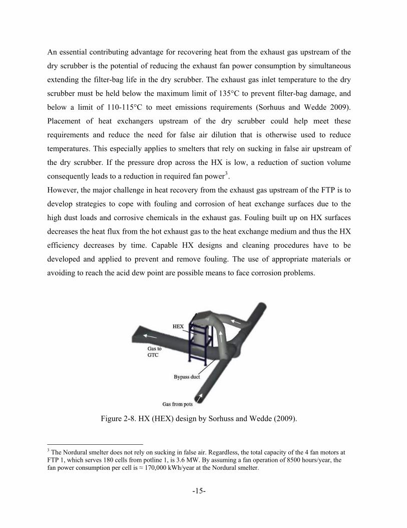
Figure 2-8. HX (HEX) design by Sorhuss and Wedde (2009).
3 The Nordural smelter does not rely on sucking in false air. Regardless, the total capacity of the 4 fan motors at FTP 1, which serves 180 cells from potline 1, is 3.6 MW. By assuming a fan operation of 8500 hours/year, the fan power consumption per cell is ≈ 170,000 kWh/year at the Nordural smelter.
-15-

-16-
Several experimental attempts on heat recovery from the exhaust gas upstream of the dry
scrubber have previously been conducted according to Sorhuss and Wedde (2009). In most
cases heavy scaling has prevented operation to continue for more than some weeks in the
previous tests. Sorhuss and Wedde (2009) observed in their previous pilot test of their new
design that less scaling in similar or even longer running periods was formed. In principle the
chosen design is a counter flow vertical HX containing several parallel pipes with water on the
outside, and exhaust gas in the inside. The hot exhaust gas enters the top of the HX, and the
water enters the bottom. Figure 2-8 shows the layout of their HX design.
However, little research work has been previously done on characterization of the particulate
content of the cell’s exhaust gas (Naess et al. 2006) and the gaseous phases, as well as the
chemical, thermal and corrosive properties of fouling layers collected on HX surfaces. The
purpose of this investigation was therefore to examine and evaluate particle characteristics,
exhaust gas properties, and fouling propensity in the gas stream in front of the dry scrubber.
The smelter under study was the Nordural smelter at Grundartangi, Iceland. Location of the
smelter and the experimental set up is shown and described in the following chapter.

3 Experimental setting
3.1 Nordural aluminum smelter, Iceland
The experiments of this research work were carried out in the Nordural smelter at
Grundartangi, Iceland (Figure 3-1). The Nordural smelter started operating in June 1998, with
an initial aluminum production of 60,000 metric tons per year. Since then the capacity has
been extended in several phases. Currently, the smelter has a capacity of 270,000 metric tons
aluminum per year which is produced in 520 prebake cells in 2 potlines, with line amperages
of 190 kA and 199 kA, respectively. The overall electric power demand of the smelter is 475
MWe, whereby the supplied electricity is exclusively produced from clean hydro- and
geothermal power. The average electricity consumption to produce one metric ton of
aluminum at Nordural is around 14.7 MWhe.
Figure 3-1. Left: Map of Iceland (Wikipedia contributors 2007), location of the Nordural aluminum smelter; right: Aerial photograph of the smelter.
The 520 pots with the prebaked anodes are fully hooded and connected to four central fume
treatment plants which clean the exhaust gas. Overhead manipulator cranes tend the pots. The
cranes are mainly used to change anodes, tap metal, and fill aluminum fluoride. A dense phase
system takes the alumina from the harbor silo to the pots. The pots are equipped with center
hoppers incorporating crust-breakers and point feeders from which alumina and aluminum
fluoride are fed. The tapped metal from the pots is transported in crucibles with 6 metric tons
-17-

capacity to the metal casting house, where it is collected in a 60 metric tons capacity furnace.
From there, the metal flows into the casting molds and solidifies as 22 kg aluminum ingots.
3.2 Location of the experimental setting
The location of the experimental setting was at the conjunction of the exhaust gas ducts
serving 180 pots on potline 1, right in front of fume treatment plant 1 (FTP 1), where the
overall duct size is around 4.5 by 5 m. The chosen site is shown on a photograph in Figure 3-2
and in an isometric drawing in Figure 3-3.
Figure 3-2. Photograph of the location for the experimental setting in front of FTP 1; the detail on the right shows the standard access flange; on the left hand side of the larger picture one can see one of the exhaust gas duct conjunctions to the 4.5 by 5 m duct in front of the dry scrubber.
The duct in front of the dry scrubber presents good conditions for dust and gas sampling, as
well as for inserting a fouling probe. There are several platforms connected to a ladder
(Figure 3-2), providing access to standard duct flanges (4 inch = 101.6 mm inner diameter), air
and electricity connection.
-18-

Figure 3-3. Isometric drawing of FTP 1 at Nordural; the arrow marks the site chosen for the experimental setting, which is also shown schematically as location A in Figure 2-7 in chapter 2.3.
3.2.1 Temperature in the duct
The temperature of the exhaust gas leaving the cells and consequently the temperature of the
total exhaust gas in front of the dry scrubber is dependent on the ambient temperature. This is
due to the fact that smelter cells are maintained with an under pressure of a few Pascal to
prevent the release of dust and gases into the pot-room. Thus, ambient air from the pot-room is
sucked into the smelter cells. The influence of the ambient temperature on the exhaust gas
temperature is highly dependent on the exhaust gas flow rate, or in other words the volume of
air sucked into the cells per time unit.
In Iceland mean ambient temperatures in winter are 10°C lower than in summer (Wikipedia
contributors 2009a). Thus, higher exhaust gas temperatures occur in the summer periods as
illustrated in Figure 3-4. The diagram shows the monthly average duct temperatures in front of
the dry scrubber 1 in 2008 and 2009 along with the monthly average ambient temperatures
observed at the smelter’s harbor weather station at Grundatangi (FAX [updated 2010]). Duct
-19-

temperatures in front of FTP 1 are measured every 5 seconds by an online monitoring system
and stored as 10 minutes average values in a database.
0
10
20
30
40
50
60
70
80
90
100
Jan. Feb. Mar. Apr. May Jun. Jul. Aug. Sep. Oct. Nov. Dec.
Tempe
rature in
°C
Months
Gas 2008
Gas 2009
Amb. 2008
Amb. 2009
Figure 3-4. Monthly average duct temperatures in front of FTP 1 and monthly average ambient temperatures at Grundatangi in 2008 and 2009.
The annual average duct temperature in 2008 was 78.6°C. However, during the course of the
study Nordural undertook a comprehensive program to better seal up the pots in order to
improve the hooding efficiency. Simultaneously the amperages of both potlines were
increased. These changes led to a significant rise in the exhaust gas temperature. For every 10
kA increase in line current a temperature increase of around 3.5-5°C can be expected
-20-

(Gylfason GH. e-mail to author. 2009 Sep 14). Thus a 2-3°C higher annual average duct
temperature can be assumed for the current smelter configuration.
The program finished at potline 1 in the end of February 2009 and at potline 2 in the end of
March 2009. Significant higher exhaust gas temperatures than in 2008 were observed in 2009
(Figure 3-4). The peak value of 109°C was reached during the day on 02.07.2009. The duct
temperatures in front of FTP 2-4 at potline 2 are in average significantly smaller than the duct
temperatures in front of FTP 1. The average duct temperature in 2008 in front of FTP 2-4 was
70.0°C.
3.2.2 Flow rate in the duct
The flow rate in the duct in front of the dry scrubber is not significantly dependent on the
ambient temperature and therefore remains almost constant through the year. Table 3-1 shows
the monthly average flow rates in front of the dry scrubber 1 in 2008, which were detected by
the online measuring system at Nordural. The small variations between monthly flow rates are
mainly due to pot operation and maintenance. The total mass flow rates listed in Table 3-1
were determined by assuming a density of 1.2 kg/m³ for the exhaust gas in the duct. This is
reasonable since the exhaust gas primarily consists of ambient air sucked into the reduction
cells.
The program to better seal up the pots described in the previous chapter has not had significant
influence to the magnitude of flow rate sucked from the cells. The flow rates per cell in potline
2 at Nordural are in average significantly higher than the flow rates in potline 1 which is
connected to FTP 1. The average volumetric flow rate per cell in potline 2 in 2008 was 1.83
Nm³/s.
-21-

Table 3-1. Monthly average duct flow rates in potline 1 in 2008. Month Volumetric flow
rate per cell[Nm³/s]
Total volumetric flow rate, 180
cells [Nm³/s]
Total mass flow rate, 180 cells
[kg/s] Jan. 08 1.58 284 341
Feb. 08 1.63 293 352
Mar. 08 1.56 281 337
Apr. 08 1.62 292 350
May 08 1.59 286 343
Jun. 08 1.57 282 338
Jul. 08 1.59 286 343
Aug. 08 1.62 292 350
Sep. 08 1.65 297 356
Oct. 08 1.62 291 349
Nov. 08 1.62 291 349
Dec. 08 1.62 292 350
Aver. 08 1.61 289 347
The following three chapters describe the experiments performed at the duct in front of FTP 1
during May and September 2009. Analysis conducted on gaseous and solid phases in the
exhaust gas are presented along with the evaluation of the results.
-22-

4 Characterization of the exhaust gas
The exhaust stream drawn from the cells contains various gaseous species and particulates,
both originating predominantly (other than air) from the smelting process. Designing a heat
exchanger for this kind of exhaust gas is challenging. The fouling process on heat exchangers
depends among others on duct flow characteristics, gas temperatures, dust particle properties
and interaction between gaseous species with particulate matter (see chapter 6.1). This chapter
will present bulk gas and particulate content, and chapter 5 will delve deeper into the particle
characterization.
4.1 Gas content
Gases present in the exhaust include predominantly air drawn in from the pot-room (as a result
of under-pressure maintained in the cells), fluorine compounds and other vapors evolved from
the electrolyte and feedstock, H2O from moisture in air, alumina, and anodes; SO2 and sulfur
compounds (e.g. H2S) from anode impurities, and CO2/CO due to anode reactions. These
gases may be corrosive for the heat exchanger materials, in particular if the water vapor in the
exhaust gas condensates.
One of the critical gas species emitted by the Hall-Héroult process is HF leaving the reduction
cells in the exhaust gas. The exhaust gas is therefore cleaned for HF in a scrubbing process in
most aluminum smelters around the world since the late 1960s. The raw material, alumina, is
used as sorbent for fluorides. The resulting chemical compound of alumina and fluoride,
called secondary alumina, is then usually collected with filter-bags (collection efficiency ≈
99%). The secondary alumina is used as feed material to the electrolyte (Grjotheim and
Kvande 1993).
At Nordural the HF concentration is measured with an online monitoring system at the inlet
and outlet of the FTP, for monitoring the efficiency of the scrubbing process. If the inlet HF
-23-

concentration is too high, saturation of the virgin alumina can be reached, which can lead to an
excessive HF emissions to the environment. At Nordural, the hydrogen fluoride concentration
of typically 250-300 mg/Nm³ in the exhaust gas coming from the cells drops down after the
FTP to typically 0.5-1 mg/Nm³ (Gudmundsson H. e-mail to author. 2009 Feb 4).
Theoretically 1.22 metric tons of CO2 ,which equals to 333 kg C, is produced per metric ton of
aluminum according to the standard equation (Lorentsen et al. 2009):
2 3 l 2 g1 3 3 Al O C Al CO2 4 4
→ (4-1)
However in practice, reduced current efficiency, anode air burn-off and anode effect
contribute to an additional 70-140 kg C per produced metric ton of aluminum. Thus, the
overall mass fraction of CO2 in the exhaust gas is in practice considerably higher than in
theory. Typically the CO2 mass fraction in the exhaust gas of modern smelters is around 1%.
Modern smelters remove most of the HF and SO2 before the residual off gases are released to
the atmosphere, but not CO2 (Lorentsen et al. 2009).
Measurements
The exhaust gas compositions were measured by using a portable flue gas analyzer (TESTO
350 M/XL) provided by the Icelandic Innovation Center (NMI) and by assessing data from the
online monitoring system in front of the dry scrubber at Nordural. The flue gas analyzer is
basically made up of a control unit, a flue gas analyzer and a flue gas probe (Figure 4-1),
which was inserted through the access flanges into the duct. The device provided by NMI is
capable of detecting CO, SO2, NO and NO2 concentrations in air and gas streams. It is built
according to the German standard DIN EN 50379-2, periodically calibrated by a technical
inspection authority and it is normally used to verify that flue gas concentrations are below
permit limits (TESTO c2009). The online monitoring system in front of all four FTPs at
Nordural measures periodically the average concentration of hydrogen fluoride (HF) in the
-24-

exhaust gas. SO2, NO and NO2 are monitored only at some stacks at the smelter
(Gudmundsson H. e-mail to author. 2009 Feb 3).
The concentration of CO2 (one of the most significant contributors to the greenhouse effect)
and water vapor (H2O), which have besides dry air the highest share of the total gas content,
were not measured since appropriate metering tools were not readily available. This may be an
opportunity for further investigation. In particular the acid dew point is of interest for heat
recovery applications.
Figure 4-1. TESTO 350 M/XL portable set up, consistent of control unit, flue gas analyzer and flue gas probe.
Results
Measurements were performed with the TESTO 350 M/XL flue gas analyzer on 04 September
2009 at two different flanges at the duct in front of the dry scrubber. Hydrogen
fluoride readings were simultaneously taken on 04 September 2009 by Nordural’s online
monitoring systems in front of the dry scrubber. The results are listed in Table 4-1.
-25-

-26-
Table 4-1. Exhaust gas composition, CO, SO2, NO, NO2, and HF measurements in front of the dry scrubber. NO and NO2 were below the lowest detection range (4 and 10 ppm) of the instrument for these two nitrogen compounds.
Sampl. time [min]
CO[ppm]
SO2
[ppm] NO
[ppm] NO2
[mg/ Nm3]
HF [mg/Nm³]
M1/ flange1
29.0 552.9 70.8 ./. ./.
239 M2/ flange4
30.3 543.3 70.6 ./. ./.
4.2 Dust content
The air and gas stream drawn from the reduction cells carries a significant amount of dust
particles. According to the operation and maintenance manual for the FTP 1 issued by ABB
Environmental on 01.04.1998 to Nordural, typical dust concentrations in the exhaust gas are
500 mg/Nm³. With the total average gas flow rate of 912 Nm³/s (see chapter 7.1) it may be
estimated that a mass of around 1600 kg dust is leaving the 520 prebake cells per hour.
Due to this heavy dust load, a detailed characterization of the free stream particles is examined
and evaluated in the following chapter and analysis of deposited particles on surfaces is
performed in detail in chapter 6.
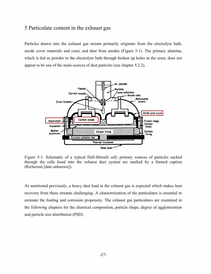
5 Particulate content in the exhaust gas
Particles drawn into the exhaust gas stream primarily originate from the electrolyte bath,
anode cover materials and crust, and dust from anodes (Figure 5-1). The primary alumina,
which is fed as powder to the electrolyte bath through broken up holes in the crust, does not
appear to be one of the main sources of dust particles (see chapter 5.2.2).
ACM and crust
Figure 5-1. Schematic of a typical Hall-Héroult cell; primary sources of particles sucked through the cells hood into the exhaust duct system are marked by a framed caption (Richerson [date unknown]).
As mentioned previously, a heavy dust load in the exhaust gas is expected which makes heat
recovery from these streams challenging. A characterization of the particulates is essential to
estimate the fouling and corrosion propensity. The exhaust gas particulates are examined in
the following chapters for the chemical composition, particle shape, degree of agglomeration
and particle size distribution (PSD).
-27-

5.1 Particle sampling
A reliable sampling procedure constitutes the first step of the particle characterization. The
goal of the dust sampling is to collect a small amount of dust from the bulk quantity, such that
this smaller fraction best represents the physical and chemical characteristics of the entire
bulk. Thus, the samples necessarily need to be representative of the bulk. The consequences of
incorrect and/or non-representative sampling can be significant and result in poor
characterization (Jillavenkatesa et al. 2001).
There are dust sampling techniques available using different mechanisms, such as settling,
impaction, inertial separation, electrical or thermal precipitation and filtration. For
microscopic analysis e.g. a double-taped specimen can be used for collecting dust in a definite
period of time; however, for a PSD analysis this would not be an appropriate method (Stern
1968).
In this study the decision was made to find a uniform sampling technique which provides a
particle sample in sufficient quantities and which can be used with all established laboratory
equipment. Such techniques are stack sampling systems that typically incorporate
combinations of probes to go into the stack and collection devices for removing the sampled
particulate matter (Stern 1968). All these stack sampling systems have in common that the
velocity in the nozzle’s tip has to be the same as the velocity of the exhaust gas; especially if
the particle size is in the range of 3-5 µm or greater (Stern 1968). The sampling with nozzle
inlet velocities that are equal to the exhaust gas velocities is called isokinetic sampling and is
described in more detail in the following chapter.
Isokinetic sampling
Particulate matter, especially in a size range of around 3-5 µm or greater (dependent on the
particle’s density, shape etc.), represents a problem in that the inertial effect on the particles
can result in erroneous samples if the sampling velocity in the nozzle’s tip is not the same as
-28-

the velocity of the exhaust gas stream at the sampling point (Stern 1968). The behavior of gas
stream lines for different ratios of duct velocity and nozzle inlet velocity is illustrated
schematically in Figure 5-2.
Figure 5-2. Behavior of stream lines for different ratios of duct velocity w and nozzle inlet velocity v in and around a sampling probe facing perpendicular to the exhaust gas stream lines (SIGRIST [date unknown]).
In the case of isokinetic sampling (w = v) the stream lines, inside and outside the nozzle, flow
in theory perpendicular to the nozzle’s cross-section, and thus particles flowing toward the
intake opening are equally collected. This results in a representative gas stream entering the
sampling apparatus. In the case of under-isokinetic sampling (w > v) heavy particles enter the
nozzle even if the stream line on which they were travelling passes by the probe; this is by
reason of their inertia. Consequently, this results in a non-representative high concentration of
coarse (heavy) particles in the gas stream entering the sampling apparatus. In the case of over-
isokinetic sampling (w < v) convergent stream lines will develop at the nozzle inlet which are
followed by light (fine) particles, but heavy particles on the outer convergent stream lines,
due to their inertia, travel past the edge of the nozzle and are not collected. This results in a
gas stream entering the probe with an excessively high concentration of fine (light) particles
(Stern 1968; Farthing and Dawes 1989; SIGRIST [date unknown]).
When stack sampling is conducted the above described error in particle concentrations due to
non-isokinetic conditions at the nozzle has to be considered. Since in practice constant,
laminar and uniform flow conditions in stacks and ducts are rather uncommon, studies have
been made on estimating the error in dust concentration dependent on the velocity ratio. In the
-29-

EPA Method 5, which is a guideline for determining particulate matter emissions, it is
proposed that an average sampling velocity should be within ± 10% of the duct velocity
(Wight 1994). Stern (1968) and Dennis et al. (1957) have shown that isokinetic sampling at
velocity ratios of 0.85-1.15 yield acceptable results with errors of measured dust concentration
in the range of 10-20%.
It can be concluded that deviations from isokinetic conditions are not desirable, but difficult to
avoid over a long time period under real sampling conditions. Velocity ratios should be kept in
a narrow range, preferable 0.90-1.10, but not outside a range of 0.85-1.15 to obtain
representative samples. The error in dust concentrations due to non-isokinetic sampling within
these velocity ratios was observed in previous studies to be around 10-20%, but can vary
between different gas streams. The error is mainly dependent on the particle size, but also on
the particle density, shape, degree of agglomeration and duct flow conditions. Studies about
isokinetic sampling rates and uncertainties related to exhaust gas streams leaving aluminum
reduction cells were not found in the literature.
Design of Isokinetic Particle Sampler
There is a wide variety of stack sampling systems available, depending on the source to be
sampled, the contaminants involved and the data desired (Stern 1968). Since it was decided to
use a stack sampling technique which provides sufficient particle quantities which could be
analyzed with laboratory equipment discussed later, an appropriate collection apparatus had to
be used. Collecting particles by using solely filters would be suitable to provide samples for
chemical analyses, but not for analyses of particle size, shape and degree of agglomeration.
Particles collected on filters would built up dense, cohesive flakes which make it impossible to
distinguish between independent, single particles. However, the use of a centrifugal collection
device, such as a cyclone, could provide representative samples in this study.
It was decided to custom design and manufacture the stack sampling system. This had the
benefit that the apparatus could be specifically designed for the sampling location at Nordural.
-30-

The piping diagram of the Isokinetic Particle Sampler is provided in Figure 5-3 and is briefly
described here:
Using vacuum built up with an air ejector, exhaust gas is drawn isokinetically through the
nozzle. Piping leads the gas stream from the nozzle to the cyclone, where solid matter is
separated from the gas stream and collected at the bottom in a container. The gas stream exits
the cyclone through the top and is passed through pre-filters and fine filters to collect fine
(light) particles, if not separated by the cyclone. The volumetric flow rate is measured with a
rotameter which is corrected for actual gas conditions using a vacuum pressure gauge and a
thermocouple. A pressure regulator is used to control and maintain the required gas mass flow
to obtain isokinetic sampling conditions at the nozzle in the duct. A ball valve upstream of the
pressure regulator is used to allow for isolation of the air supply.
The duct velocity is measured using a Pitot tube in combination with a manometer before each
sampling run, and the temperature and static pressure in the duct is detected using Nordural’s
online measuring system.
Figure 5-3. Piping diagram of the Isokinetic Particle Sampler.
In the following, details are given for the velocity measurement set up and for each component
of the Isokinetic Particle Sampler. The design, availability, cost and producibility of each
component are considered and described.
-31-

VELOCITY MEASUREMENT SET UP
A Pitot tube in combination with a manometer was used to determine the gas velocity in the
duct before each sampling run. The Pitot tube is of appropriate small size for insertion through
the access flange. For reaching distances as far as 1.3 m in the duct, the Pitot tube was taped to
a galvanized tube of 1800 mm length with outer diameter of 34 mm and inner diameter of 27
mm (Figure 5-4, top).
At the opposite end to the Pitot tube, a 90° elbow was welded to the extension tube (Figure 5-
4, left bottom). The elbow and the Pitot tube nozzle are parallel to each other. Thus, the 90°
elbow allows an accurate positioning of the Pitot tube from outside the duct (Figure 5-4, right
bottom). The Pitot tube obtains proper results if the nozzle is pointed parallel to the exhaust
gas stream lines (no yaw).
Figure 5-4. Top: Front view of Pitot tube fastened to extension tube and connected to two long rubber hoses; left bottom: 90° elbow welded to extension tube; right: Access flange at Nordural with extension tube inserted to the duct in front of the dry scrubber.
By having one inlet hole in the front and several small inlet holes in the outer cylinder, the
Pitot tube can measure the dynamic pressure of the exhaust gas in combination with a
-32-

manometer. The manometer used in the present case is a simple apparatus with liquid column
(see Figure 5-12) showing the gauge pressure in inches of water. By use of the ideal gas law
and the Bernoulli equation, the gas velocity can be calculated from the detected dynamic
pressure, the duct temperature and the static pressure in the duct. The molar mass of the gas is
assumed to be that of clean air.
The exhaust gas velocities were measured before each sampling run at the sampling point
itself and a few centimeters around that point - whereby no significant velocity deviations
between these points were obtained. The exhaust gas velocity was on average 14 m/s in May
and Sept. 2009, and 17.5 m/s in the summer months 2009. It was found that the exhaust gas
velocity cyclically alternated by around 3.5 m/s with a period of a few seconds due to the
operation of the filter-bags in the dry scrubber. Due to the cyclically velocity alternation, the
isokinetic sampling velocity was set to the average exhaust gas velocity.
SAMPLING PROBE (NOZZLE + BEND)
The nozzle was built from a tapered plastic tube and taped perpendicular to the extension tube.
A plastic hose with 5 mm inner diameter was connected to the nozzle ending. The hose was
bent such that it does not deform during sampling (due to the hot temperatures in the duct) and
that particles experience as little resistance as possible in the conduit (Figure 5-5, top). Both
criteria are fulfilled by having a long radius bend. The use of an elastic plastic hose instead of
a metal pipe for the long radius bend has the benefit that the probe still can be inserted into the
duct, even though the dimensions of the probe’s bend exceed those of the access flange. The
plastic hose is fastened to the extension tube right after the bend ending. In addition a plug
connection is fixed close to the bend to enable a quick removal or exchange of hoses.
Previous studies have shown that a too small nozzle diameter at the tip can lead to errors in the
sampled dust concentration. The American Society of Mechanical Engineers (1957) mentions
the importance of a nozzle diameter of not less than 1/4 inch (6.35 mm), whereby the tapering,
if any, should be on the outside, not on the inside. However, Hemeon and Haines (1954) found
that for particles in the 5-25 µm size range there was little deviation in sample weights
collected with each of the three nozzles used; 1/8 (3.18 mm), 1/4 (6.35 mm) and 3/8 (9.53
-33-
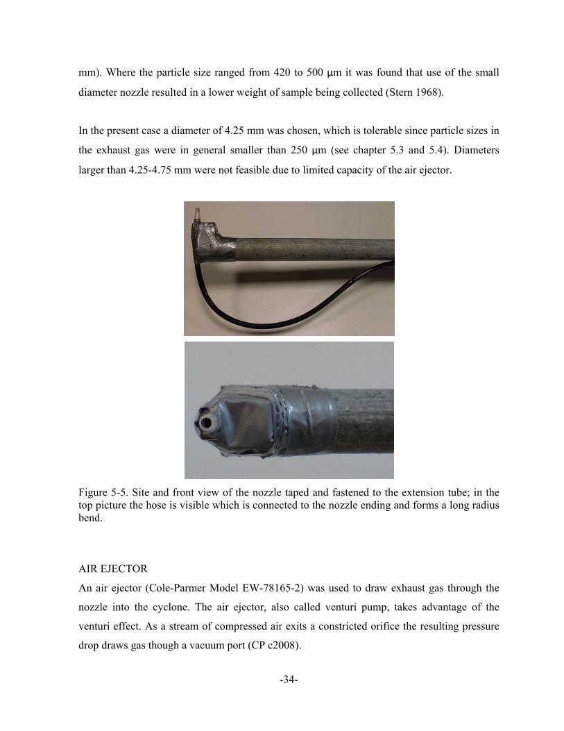
mm). Where the particle size ranged from 420 to 500 µm it was found that use of the small
diameter nozzle resulted in a lower weight of sample being collected (Stern 1968).
In the present case a diameter of 4.25 mm was chosen, which is tolerable since particle sizes in
the exhaust gas were in general smaller than 250 µm (see chapter 5.3 and 5.4). Diameters
larger than 4.25-4.75 mm were not feasible due to limited capacity of the air ejector.
Figure 5-5. Site and front view of the nozzle taped and fastened to the extension tube; in the top picture the hose is visible which is connected to the nozzle ending and forms a long radius bend.
AIR EJECTOR
An air ejector (Cole-Parmer Model EW-78165-2) was used to draw exhaust gas through the
nozzle into the cyclone. The air ejector, also called venturi pump, takes advantage of the
venturi effect. As a stream of compressed air exits a constricted orifice the resulting pressure
drop draws gas though a vacuum port (CP c2008).
-34-

The present air ejector has a free-air capacity of 34.0 l/min (LPM) and can obtain a maximum
vacuum of 28” Hg (0.9464 bar). It requires no electricity, but merely a pressurized air
connection, which was available adjacent to the sampling location (CP c2008).
CYCLONE
A cyclone was used for separating particles from the gas stream and collecting them in a
container at the bottom of the unit. The function principle and the principal design of a
cyclone is illustrated in Figure 5-6.
Figure 5-6. Left: Schematic of a cyclone illustrating the function principle of the centrifugal separator; right: Schematic of a cyclone labeled with main dimensions which influence the collection efficiency (Ramachandran et al. 1991; EPA 2005).
-35-

A cyclone is basically a settling chamber in which gravitational forces are replaced or
supported by centrifugal forces. Air enters the cyclone tangentially, creating a tangential jet
(vortex flow pattern). The jet forces the flow against the outer wall of the centrifugal
separator. With an increase in tapering at the lower body of the cyclone, the air spirals faster in
the separator and thus the centrifugal forces increase. The dust particles, by virtue of their
inertia, will tend to move toward the outside separator wall from which they are led into a
collection container at the bottom. Like common cyclones in nature, when the cyclone’s spiral
reaches the bottom it reverses and a smaller diameter vortex spins in direction of the cyclone’s
top. As separated particles move down into the collection container where they are retained,
large samples can be collected with little increase in pressure drop during operation (Perry and
Chilton 1973; EPA 2005).
The centrifugal separating force in a cyclone may range from 5 times gravity in very large
diameter, low-resistance cyclones, to 2500 times gravity in very small, high resistance units.
(Perry and Chilton 1973). Since centrifugal forces are greater than gravitational forces,
cyclones can be operated in any orientation.
The primary design factor that can be utilized to control the collection efficiency is the
cyclone’s body diameter. A unit with smaller body diameter operating at a fixed pressure drop
will have the higher efficiency due to higher generated centrifugal forces. (Perry and Chilton
1973; Gimbun et al. 2004). It is generally accepted that the cut-off diameter is proportional to
the square root of the cyclone’s body diameter (Gimbun et al. 2004). The cut-off diameter of
the cyclone is defined as the particle diameter corresponding to 50% collection efficiency.
Thus it is an indicator of the size range of particles that can be collected (Perry and Chilton
1973; Kuo and Tsai 2001; Gimbun et al. 2004).
Apart from the body diameter, the collection efficiency of a cyclone depends on several
factors, such as the other main dimensions of the centrifugal separator shown in Figure 5-6,
particle density, and operating temperature. The fluid’s density and viscosity, as well as
operating parameters, such as the inlet velocity of the fluid into the cyclone and the outlet
conditions, also affect the collection efficiency (Gimbun et al. 2004). Theoretical and practical
-36-

studies have shown that the collection efficiency increases significantly with decreasing
cyclone body diameter, operating temperature, and cyclone inlet and outlet width.
Furthermore, the collection efficiency increases proportionally with inlet velocity and particle
density. (Perry and Chilton 1973; Gimbun et al. 2004). However, a too high inlet velocity
would decrease the collection efficiency because of too strong turbulence and resultant re-
entrainment of particles. The range of practicable cyclone inlet velocities is around 15-30 m/s
and the optimum cyclone inlet velocity is around 18 m/s (Gimbun et al. 2004).
Cyclone collection efficiencies can reach 99% for particles bigger than 5 µm. In certain cases
efficiencies as high as 98% have been realized on dusts having an ultimate particle size of 0.1
to 2.0 μm because of the predominant effect of agglomeration (Perry and Chilton 1973;
Gimbun et al. 2004).
Table 5-1. Dimensions (Fleer) used in this study; and comparison of the Stairmand dimension ratios with the used dimension ratios (Fleer). The dimensions are shown qualitatively in Figure 5-6.
Dimensions in mm
D De S h H B a b
Fleer 61.5 30.0 … 4.0 35.0 95.0 175.0 22.0 ø 4.0 ø 4.0Dimension‐less ratios
./. De/D S/D h/D H/D B/D a/D b/D
Stairmand ./. 0.50 0.50 1.50 4.00 0.375 0.500 0.200Fleer ./. 0.49 … 0.065 0.55 1.54 2.85 0.358 0.065 0.065
The Stairmand high efficiency cyclone is one of the standard cyclone designs and is most
commonly used. The relative dimensions of a Stairmand high efficiency cyclone are
a=S=De=0.5D, b=0.2D, h=1.5D, H=4D, and B=0.375D (Kuo and Tsai 2001). The decision
was made to build a cyclone which has similar dimensions ratios as the Stairmand high
efficiency cyclone. It was build from pre-fabricated plastic bottles, since they are inexpensive,
available in many varieties in public stores, and easy to modify. In addition, the transparency
of the plastic material enabled observation of the performance during test runs in the
laboratory and at the aluminum smelter. Due to practical lessons learned the dimensions listed
-37-

in Table 5-1 were used. The dimension ratios are also shown and compared to the standard
Stairmand type in that table.
The tangential inlet was chosen to be cylindrical and the inner tube with 30 mm diameter was
reduced at the top of the cyclone to 4 mm tubing (inner diameter). This design of the inlet and
outlet proved to be easily connectable to the sampling hoses and simultaneously provided high
inlet and outlet velocities. As mentioned earlier, the inlet velocity has to be in a certain range.
In the present case the chosen inlet diameter of 4 mm results in an average inlet velocity of
around 20 m/s in summer months (with 4.25 mm nozzle tip diameter). The pressure drops due
to the narrow inlet and outlet were tolerable. The collection unit, which can easily be
demounted from the cyclone’s bottom, is a standard 50 ml container with screw cap used in
laboratories.
Several models, such as the Lapple, Koch and Licht, Li and Wang, and Iozia and Leith model,
can be used for predicting cyclone collection efficiencies (Gimbun et al. 2004). By using the
Lapple model (Appendix A), described in Perry and Chilton (1973) and Gimbun et al. (2004),
the cut-off diameter of the cyclone was determined to be in the range of 0.2 to 0.4 μm
assuming a particle density range of 800 to 4000 kg/m3. Thus particles larger than 2.5 to 5 μm
are predicted to be separated from the gas stream with 99.3% certainty.
Independently from the theoretical predictions, the collection efficiency was verified by
checking the filters downstream of the cyclone for buildup. For several sampling runs in
summer 2009 the buildup on the filters accounted for around 20-30% of the total mass
collected. The overall collection efficiency of the cyclone is consequently between 70-80% for
these gas streams. However, it should be noted that some particles smaller than 0.45 μm may
not have been collected, neither with the cyclone nor with the filters.
A future strategy for increasing the cyclone’s collection efficiency is to use steel as
construction material. This requires a more complex fabrication of these separators, with
higher costs, but it allows for an almost unconstrained design in dimension ratios. In
particular, the use of steel enables smaller cyclone body diameters due to more accurate
-38-

manufacture opportunities. Design consideration for these kind of cyclones with body
diameter down to 17.5 mm can be found in Kenny and Gussmann (2000).
In addition, cyclones with small body diameter for aerosol sampling and emission control are
commercially available. These cyclones are often offered with modifiable compounds, like the
one shown in Figure 5-7, to adjust for different conditions in different gas streams. The
cyclone set shown on the photograph, is designed for in-stack sampling. It is offered with
several nozzles having different tip diameters. In addition a second, smaller centrifugal
separating unit and a back up filter unit can be optional mounted downstream to the actual,
bigger cyclone for finer particle collection.
Figure 5-7. Commercially available cyclone set for aerosol sampling and emission control (NSE c2004).
Finally, the location for placing the cyclone needed to be chosen. There were basically two
locations for placing the cyclone:
1. Inside the duct, close to the probe’s nozzle and fastened to the extension tube
2. Outside the duct, e.g. fixed to a compact, transportable support.
The major disadvantage in using the latter approach is the length of pipe between the nozzle
and the collecting device, in which material deposition can occur. Such probes should be
frequently flushed with compressed air. The error introduced by deposition of materials in the
probe and tubing is eliminated with the use of the first mentioned version, where almost no
piping is required between the nozzle and the cyclone (Stern 1968).
-39-

However, approach 1 requires that the cyclone dimensions are smaller than those of the access
opening to the stack or duct. In the present case the opening is the access flange with inner
diameter of 101.6 mm (see Figure 3-2). Consequently the cyclone had to be located outside
the duct since the unit’s size with all connections exceeded this limitation. However,
experience had shown, that using plastic hoses in combination of flushing the system after
each sampling run, resulted in few deposits remaining in the tubing upstream of the cyclone.
In addition, the transparent material of both the cyclone body and the collection container
allowed for checking and monitoring the sampling process during operation from outside the
duct.
PRE-FILTERS AND FINE FILTERS
Two different types of filters connected in series were used downstream of the cyclone to
collect any fine (light) particles which were not separated by the centrifugal device. By this
mean clogging of the components downstream of the filters was prevented and determining
the cyclone collection efficiency is feasible, as described earlier.
Reasons for a multiple use of filters are that two main criteria have to be fulfilled. On one
hand the filtration should provide sufficient collection efficiencies which are obtained by the
right choice of fine filter media, but on the other hand it should provide tolerable pressure
drops, even if the filter media gets significant particle buildup during the sampling run.
Figure 5-8. Photograph of a typical used pre-filter; the exhaust gas inlet is on the right side; the fuel-filter illustrated on this picture was used during the sampling on 14 August 2009; a noticeable built up of particles is observable.
-40-

If the filter media is too fine and the filter media area is too small, than large pressure drops
led results in air ejector capacity being insufficient to obtain the required sampling mass flow,
even if the filter media is clean. For this reason a standard fuel-filter, which has the
characteristic of a large filter area, was used as a pre-filter (Figure 5-8). The large filter area
assures small pressure drops, even if the filter paper gets noticeable particle buildup.
Four in parallel connected fine filters of type Millipore, Millex-HV, PVDF 0.45 microns
(Figure 5-9) were connected in series with the pre-filter to guarantee a filtration down to 0.45
microns. The connection of four filters in parallel leads to an increase of the total filter area,
providing a lower pressure drop over the filter set before and during sampling. The 0.45
micron filters were connected in parallel by using transparent rubber hoses and plastic Y-
connections. The inlet of the filters were connected with threads to junctions, which allowed
for a buildup check by disconnecting them.
Figure 5-9. Photograph of 0.45 micron filters connected in parallel by the use of transparent rubber hoses and plastic Y-connections; the exhaust gas inlet is on the right side
ROTAMETER
The gas flow rate was measured with a rotameter (Cole-Parmer WZ-32030-15) corrected for
gas conditions using a vacuum pressure gauge and a type T thermocouple. A rotameter
measures the volumetric flow rate of liquid or gases by use of a drag ball (float) floating in a
tube which has an inlet and outlet on both endings. The tube is positioned vertically so that
gravity forces and lifting forces act perpendicular on the drag ball (float), whereby both forces
act in opposite directions (Figure 5-10). The drag ball reaches an equilibrium position where
-41-

the upward force of the flowing fluid equals the downward force of gravity. A scale on or next
to the tube allows for reading the equilibrium point.
Figure 5-10. Function principle of a rotameter; the float reaches an equilibrium position where the upward force of the flowing fluid equals the downward force of gravity (Scheer c2009).
The rotameter used in the present case has a scale in LPM (2-42 LPM range), whereby it was
calibrated for air at 70 F (21.1°C) and 1 ATM (101,325 Pa). By adopting the ideal gas law,
the calibration density ρcal was 1.2 kg/m³. If the density right after or in front of the rotameter
ρrota is known, then the mass flow of the flowing fluid mfluid can be calculated using following
equation:
rotafluid rota cal
cal m V ρ
⋅ ρ ⋅ρ
&& (5-1)
For experimental runs the fluid mass flow through the rotameter and all other components
were determined by the fixed nozzle tip diameter (4.25 mm) and the exhaust gas conditions in
the duct. The volumetric flow rate, which the rotameter had to display to obtain constant
isokinetic conditions at the nozzle, was determined with the equation above. Since the mass
flow rate cannot be determined until having performed the velocity, temperature and static
pressure measurements at the duct and since the pressure and the temperature at the rotameter
vary during sampling operation, an excel sheet was used on site for calculating the required
volumetric flow rate at the rotameter. The excel sheet is attached to the appendix (Appendix
B).
-42-

THERMOCOUPLE
A thermocouple of type T in connection with a data logger (OMEGA OM-DAQPRO-5300)
was used to detect the sampling temperature downstream of the rotameter. A thermocouple
consists of two dissimilar metals, joined together at one end. When the junction of the two
metals is heated or cooled a voltage is produced that can be correlated back to the temperature
of the heat source (OA c2009). The measured temperature was used for correcting the
rotameter flow rate readings.
PRESSURE GAUGE
A standard vacuum pressure gauge (Ashcroft; accuracy 0.25%) was used to detect the pressure
downstream of the rotameter relative to the atmospheric pressure. It was observed that the
pressure downstream of the rotameter sometimes varied during sampling runs. It could vary
due to particle built up on filters and deposits in tubing, connections and components. Gas
entering the probe’s nozzle has self-evidently the same mass flow as the gas going through the
rotameter. However, the volumetric flow is different at both locations. Usually the volumetric
flow through the rotameter is much higher than at the nozzle’s tip due to a significant pressure
drop in the sampling system; the temperature drops as well, but is in this case less sensitive to
the volumetric flow than the pressure. Consequently, it is necessary to monitor the pressure at
the rotameter and to adjust the volumetric flow readings, with recalculations of the excel sheet
(Appendix B).
PRESSURE REGULATOR
A pressure regulator was used to control the pressure and simultaneously the mass flow of the
compressed air entering the air ejector. The compressed air is cleaned in the regulator and was
controlled by an integrated valve. It is important for isokinetic sampling that a fixed mass flow
through the sampler is maintained even though the pressure drop increases due to deposit built
up on the filters, hoses and connections. Maintaining the fixed gas mass flow during sampling
was performed with the pressure regulator by manually adjusting/controlling the air mass flow
and pressure entering the air ejector.
-43-

BALL VALVE
A standard ball valve was used to allow for quick disconnection from the compressed air
source. Thus, the ball valve enables a quick safety shut down during sampling runs and
modification periods.
PIPING AND CONNECTIONS
For piping plastic and rubber hoses with inner diameters of 5 mm were used. Components and
hoses were connected with appropriate junctions made out of plastic, rubber or stainless steel.
Sagging of hoses was tried to be avoided by cutting the hoses to appropriate short lengths, as
seen in Figure 5-13. This has the additional, positive side effect of lower pressure drop in the
piping system due to free flow conditions and shorter distances. Experience showed that hoses
with an inner diameter of around 5 mm showed advantages in comparison to hoses with
smaller or greater inner diameters:
Relatively high velocities (12 > m/s) which lead to a small boundary layer in the
tubing and to lower particle deposition in the hoses and junctions
Tolerable pressure drops
Medium flexibility and stability
Easily connectable to most of the components
Available in most hardware stores
Low costs
In addition experience showed that rubber hoses were very easy to connect to components due
to their flexibility and they enable an in situ observation of deposit built up in the piping
system. However, they get softer and therefore more easily squeezed and loosened in a hot
environment, they have a higher flow resistance, and they tend to get quicker particle
depositions. These disadvantageous characteristics of a rubber hoses are not present in a
plastic hose, whereas this kind of tubing have the drawback of being less elastic.
Consequently, a combination of both tubing types was used as visible in Figure 5-12 and
Figure 5-13. Sampling hoses leading to the cyclone were blown down with compressed air
between each run to collect any deposited particles.
-44-

EXTENSION TUBE
An extension tube was used to support the probe (see Figure 5-14), and to reach sampling
points in the duct which assure an equal flow distribution of the exhaust gas stream lines. The
extension is a standard galvanized tube with 34 mm outer diameter and 27 mm inner diameter;
and a length of 1450 mm. A blind flange having the same dimensions as the access flange at
the duct, was welded to the extension tube to assure constantly a parallel position of the nozzle
to the exhaust stream lines (see Figure 5-15). The nozzle was supported by a elbow welded to
the end of the extension tube (Figure 5-11). The position of the blind flange on the extension
tube was chosen, so that the distance between nozzle and inner duct wall is 1125 mm. The
design of the extension tube has the following benefits:
It allows multiple sampling from different access flanges
It guarantees sampling under an equal flow distribution of the exhaust gas stream lines
due to a sufficient distance of the nozzle from the inner duct wall (sufficient
penetration to avoid wall effects)
It enables low-vibrating conditions at the sampling nozzle due to the stiff construction
and the relatively short lever.
Figure 5-11. Schematic of the extension tube; dimensions are given in millimeters.
-45-

ASSEMBLY OF THE COMPONENTS
Figure 5-12 and Figure 5-13 show the components of the Isokinetic Particle Sampler mounted
on a transportable, wooden support. Components shown in both photographs are the cyclone,
the pre-and fine filters, the rotameter, the vacuum pressure gauge, the data logger connected to
the T-thermocouple, the pressure regulator connected to the ball valve and pressurized air
hose, the air ejector and the manometer. Latter one was used in combination with the Pitot
tube for velocity measurements. All components are also shown schematically in the pipe
diagram in Figure 5-3.
Figure 5-12. Front view of the wooden support of the Isokinetic Particle Sampler positioned on the platform in front of the dry scrubber at Nordural.
-46-

On the side view of the Isokinetic Particle Sampler shown in Figure 5-13, one can see the
cyclone inlet connected with the plastic hose leading to the probe in the duct. The blind flange
mounted to the access flange at the duct is observable on the right top of the photograph.
All components and connections were checked for air tightness before assembling them.
Experience showed that the critical components prone to leakages are the cyclone, the in series
connected pre-filter and fine filters and all used connections. These units were checked for
leakages by pressurizing them under water. Typical run duration was 2-3 hours to collect a
sample of about 0.5 gram with the cyclone.
Figure 5-13. Side view of the wooden support of the Isokinetic Particle Sampler.
-47-

Measuring dust concentration
In addition to particle sampling, experiments were performed to detect the dust concentration
in the exhaust gas. For this purpose, the cyclone was disconnected and a filter set was
connected straight with the rotameter. As mentioned in the previous chapter, a too long
distance between the nozzle and the collecting device can introduce an error due to deposition
of solid matter in the tubing. Thus, the collection device (filter set) was positioned on the
extension tube, close to the nozzle.
A filter set similar to the one used in the Isokinetic Particle Sampler was applied. Thus, a
standard fuel-filter was used as a pre-filter and four in parallel connected fine filters of type
Millipore, Millex-HV, PVDF 0.45 microns were connected in series with the pre-filter.
However, the connections and hoses were kept as short as possible to ensure an appropriate,
compact size of the collection system which can be fastened to the extension tube – whereby
the existing extension tube from the Isokinetic Particle Sampler could be used without
required removal or modification of the nozzle and bend (Figure 5-14 and Figure 5-15).
The plug connection close to the bend enables a quick, destructive disconnection of the filter
set inlet. An additional plug connection fastened to the extension tube close to the filter set
outlet serves the same function.
The entire collection system (filters + hoses + junctions), which is connected in between these
two plug connections, was weighted before and after each sampling run. It was heated for two
hours in a 60°C oven and then cooled down to ambient temperature in an vacuum bowl for 30
minutes, before it was weighted on an accurate scale in the laboratory (NMI). This procedure
guaranteed a similar moisture content in the collection system before and after the sampling.
-48-
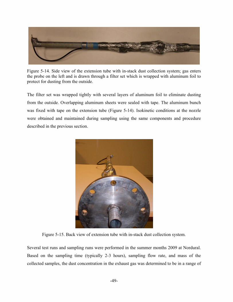
Figure 5-14. Side view of the extension tube with in-stack dust collection system; gas enters the probe on the left and is drawn through a filter set which is wrapped with aluminum foil to protect for dusting from the outside.
The filter set was wrapped tightly with several layers of aluminum foil to eliminate dusting
from the outside. Overlapping aluminum sheets were sealed with tape. The aluminum bunch
was fixed with tape on the extension tube (Figure 5-14). Isokinetic conditions at the nozzle
were obtained and maintained during sampling using the same components and procedure
described in the previous section.
Figure 5-15. Back view of extension tube with in-stack dust collection system.
Several test runs and sampling runs were performed in the summer months 2009 at Nordural.
Based on the sampling time (typically 2-3 hours), sampling flow rate, and mass of the
collected samples, the dust concentration in the exhaust gas was determined to be in a range of
-49-
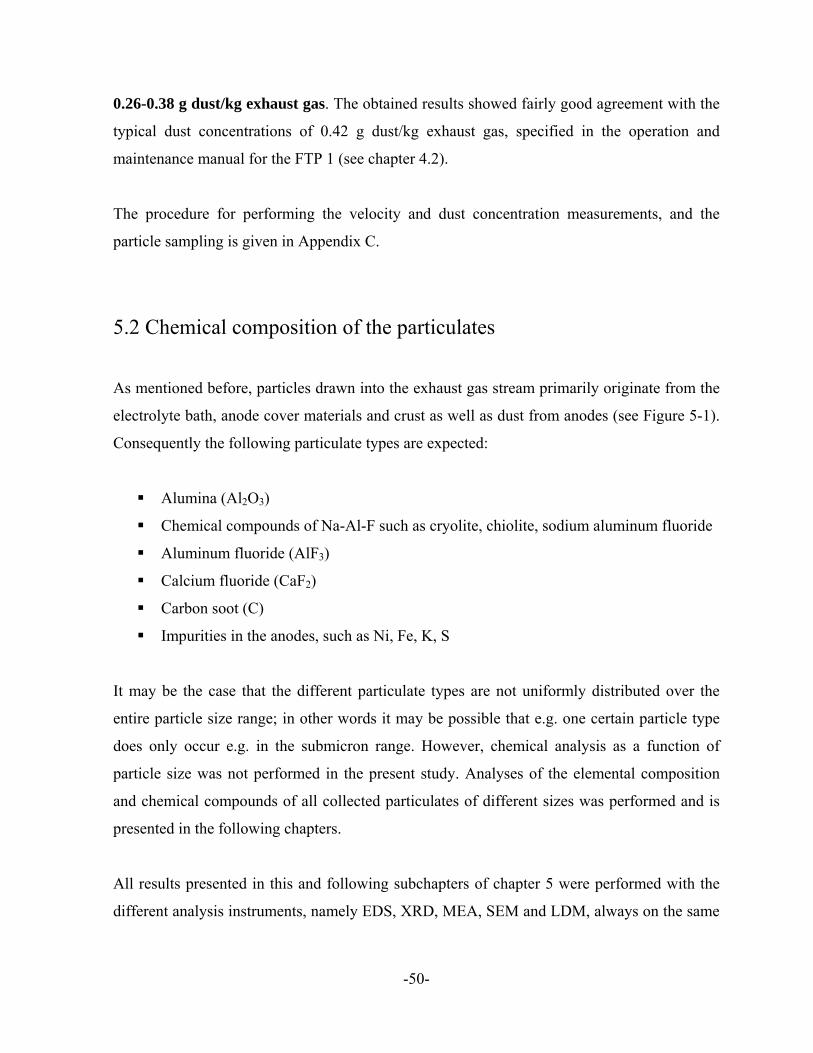
0.26-0.38 g dust/kg exhaust gas. The obtained results showed fairly good agreement with the
typical dust concentrations of 0.42 g dust/kg exhaust gas, specified in the operation and
maintenance manual for the FTP 1 (see chapter 4.2).
The procedure for performing the velocity and dust concentration measurements, and the
particle sampling is given in Appendix C.
5.2 Chemical composition of the particulates
As mentioned before, particles drawn into the exhaust gas stream primarily originate from the
electrolyte bath, anode cover materials and crust as well as dust from anodes (see Figure 5-1).
Consequently the following particulate types are expected:
Alumina (Al2O3)
Chemical compounds of Na-Al-F such as cryolite, chiolite, sodium aluminum fluoride
Aluminum fluoride (AlF3)
Calcium fluoride (CaF2)
Carbon soot (C)
Impurities in the anodes, such as Ni, Fe, K, S
It may be the case that the different particulate types are not uniformly distributed over the
entire particle size range; in other words it may be possible that e.g. one certain particle type
does only occur e.g. in the submicron range. However, chemical analysis as a function of
particle size was not performed in the present study. Analyses of the elemental composition
and chemical compounds of all collected particulates of different sizes was performed and is
presented in the following chapters.
All results presented in this and following subchapters of chapter 5 were performed with the
different analysis instruments, namely EDS, XRD, MEA, SEM and LDM, always on the same
-50-

sample, drawn on 14 August 2009 at Nordural, to enable a correlation and comparison
between these obtained results. This sample was drawn for 126 min with a sampling mass
flow of 2.35*10-4 kg/s. The mass collected by the cyclone was 0,4373 g and 0,16 g collected
by the filters.
5.2.1 X-Ray Energy Dispersive Spectrometer (EDS)
Elemental analysis was performed using an X-ray Energy Dispersive Spectrometer (EDS).
The EDS used in this study is a built-in instrument of the Field Emission Scanning Electron
Microscope (SEM), of type Zeiss Supra 25 (Figure 5-16). The instrument is owned by the
Icelandic Innovation Center (NMI). EDS analyses were performed with assistance of
specialists at NMI.
Specimens
Specimen holders
Figure 5-16. Left: Field Emission Scanning Electron Microscope (SEM), of type Zeiss Supra 25 with built-in X-ray Energy Dispersive Spectrometer (EDS); right: Specimen holders and specimens. Specimens on the picture are already prepared for EDS and SEM analysis.
EDS is an analytical technique which utilizes the X-rays that are emitted from the specimen
surface while bombarded by a high electron beam (here: cobalt beam). When the specimen is
hit by the high energy electrons, the atoms on the specimen surface are excited to a higher
energy level. When they fall down to their ground state, the atoms emit an X-ray at
-51-

wavelengths which are characteristic for the atoms from which they come. The X-ray detector
measures the number of these emitted X-rays versus their energy. Then a spectrum of the
energy versus relative counts of the detected X-rays is obtained by the EDS software (see
Figure 5-18) and a qualitative and quantitative determination of the elements present in the
sample is possible (Herguth and Nadeau [date unknown]).
The EDS specimens were prepared by equally and densely distributing the sampled particles
on an adhesive carbon background (see Figure 5-17). Registered standards (MAC [date
unknown]) were used and average weight percentages for detected elements were normalized
to 100%. Due to the irregular size of the particles a non-uniform surface was inevitable and
custom standards reflecting the predicted compositions could not be prepared a priori. Thus,
the quantitative results from the EDS can contain significant uncertainty and should be used
for qualitative comparison between elements and samples rather than for firm quantitative
analysis. Especially the use of non-custom standards, which are not similar to the material
under consideration, can result in a significant uncertainty (Johansson B. e-mail to author. 23
2009 Mar 23). Getting these custom standards is difficult to obtain, and was thus not
considered in the present study.
However, experiences made during the course of the study have shown that results of the EDS
analysis are consistent. The measurement results obtained on different areas on the same
specimen (see Figure 5-17) are in very good agreement with each other. Even when new
specimens were prepared with the same sample at a later day, these measurement results
showed very good agreement with the former ones.
Results
For identifying the elemental composition of the particle sample, four rectangular areas on the
same specimen were analyzed with the EDS. A SEM image showing a part of the examined
EDS specimen along with area no. 1 is illustrated in Figure 5-17. The magnified image
demonstrates clearly the densely distributed particles on the specimen and the relatively
smooth surface. Figure 5-18 shows the EDS spectrum. The energy (x-axis) versus relative
-52-

counts (y-axis) of all detected X-rays emitted from the particle sample (here: area no. 1) are
displayed in this spectrum.
Figure 5-17. SEM image showing part of the examined specimen, and area no. 1 (rectangular area) which is hit by the cobalt electron beam during the EDS analysis to induce a quantum jump on the atoms shells.
Figure 5-18. EDS spectrum of elements detected in the sample on area no. 1; the x-axis shows the energy in keV and the y-axis the relative counts of the detected x-rays.
-53-

The elemental composition of the particles sampled in front of the dry scrubber is shown in
Table 5-2. As mentioned in the previous chapter, the quantitative results should be used for
qualitative comparison between elements rather than for firm quantitative analysis. A
qualitative evaluation of the EDS results is performed below:
Carbon (C), oxygen (O), fluorine (F) and aluminum (Al) are present in a considerable
amount
Sodium (Na) is very notable, but likely less abundant than C, O, F and Al
Sulfur (S), potassium (K) , calcium (Ca), iron (Fe) and nickel (Ni) are present, in a
small amount
Sulfur (S), iron (Fe), nickel (Ni) and potassium (K) are likely impurities of the carbon-anodes,
but may also originate in small quantities from the pot-room dust which is sucked into the
reduction cells.
Table 5-2. Elemental composition of sampled particles determined with the EDS; measurements were performed on 4 different areas on the same specimen. The average of the 4 measurements is normalized to get a 100% total sum of all elemental weight shares (see rightmost column).
Element Area 1 [weight %]
Area 2[weight %]
Area 3[weight %]
Area 4[weight %]
Average [weight %]
Normalized average
[weight %] C 58.69 57.97 54.82 60.41 57.97 37.3
O 37.49 36.51 35.79 38.48 37.07 23.9
F 25.96 25.34 24.22 26.74 25.57 16.5
Na 8.41 8.42 8.10 8.36 8.32 5.4
Al 24.14 22.46 23.13 23.94 23.42 15.1
S 0.83 0.80 0.73 0.83 0.80 0.5
K 0.16 0.14 0.14 0.12 0.14 0.1
Ca 0.36 0.32 0.39 0.44 0.38 0.2
Fe 0.75 0.74 0.65 0.69 0.71 0.5
Ni 0.87 0.85 0.95 0.68 0.84 0.5
Total 157.66 153.69 149.05 160.70 155.28 100.0
-54-

5.2.2 X-Ray Powder Diffractometer (XRD)
An X-Ray powder diffractometer (Bruxer AXS D8 Focus) was used to identify the different
crystalline phases. The Icelandic GeoSurvey institution (ÍSOR) provided the XRD shown on
Figure 5-19 and assisted the analysis process.
The principle of the X-ray (powder) diffractometer is based on Bragg’s law, which states that
depending on the atomic arrangement, interferences arise from X-rays scattered by a crystal.
The interferences are constructive when the path difference between two diffracted X-ray
waves differs by an integral number of wavelengths (EP [date unknown]).
The XRD software generates a graphical displayed pattern of the analyzed sample (see Figure
5-20), which can subsequently be manually scanned for candidates of possible occurring
crystalline phases and presence of amorphous material. The proportion of the occurring
crystalline phases and the amorphous material can be evaluated qualitatively with the
graphical pattern.
The specimens were prepared by grinding a small amount (< 0.1 g) of the sampled particles to
a fine, homogenous powder with pestle and mortar (Figure 5-19). Then, the fine powder was
distributed on a squared quartz plate (sample holder) by using Acetone until a smooth, thin
and dense layer was formed.
The relatively small particle sample (< 0.1 g) analyzed with the XRD may lead to small errors
in the generated pattern of the crystalline phases. If samples in larger quantities (> 0.5 g) are
available, then different sample holders can be used for more accurate analysis of the
crystalline phases. Samples in such quantities were not available with sampling equipment
used in this study.
-55-

Figure 5-19. Left: X-Ray powder diffractometer (Bruxer AXS D8 Focus) at ÍSOR; right: Pestle and mortar for grinding particle samples to a fine, homogenous powder.
Results
The pattern of the dust sample generated with the XRD software is shown in Figure 5-20. The
x-axis shows the 2-Θ (Theta) scale which is the angle between the diffracted X-ray beam and
the direction of the incident X-ray beam (EP [date unknown]). The y-axis is presented in
relative counts. The highest peaks in Figure 5-20 are produced by corundum (alumina) phases.
Amorphous material is notable in the sample due to the raised background and the appearance
of a broad hump between 20-30° on the 2-Θ (Theta) scale. Following, qualitative observations
can be obtained from the pattern:
Alumina (Al2O3) is in considerable quantity as crystallized corundum
Cryolite (Na3AlF6) is present in considerable amount
Chiolite (Na5Al3F14) is well crystallized and very notable
Kogarkoite (Na3(SO4)F) is producing a significant peak at 2Θ=18.3° and is therefore
very noticeable
-56-

Fluorite (CaF2) is found in small amount
Sodium aluminum fluorite (NaAlF4) can also be found in small amount
Other crystalline phases are not in notable quantities to be identified
Non-crystalline phases (amorphous material) are present in noticeable amounts
Lin
(Cou
nts)
0
100
200
300
400
500
600
700
800
900
1000
1100
1200
1300
1400
1500
2-Theta - Scale4 10 20 30 40 50 60 7
NaAlKog
FluCryCry
ChiChi
AluAluAlu
NaAl
ChiCry
AluAluAlu
Chi
isokinetic
Figure 5-20. XRD analysis of the isokinetic sample drawn at the duct in front of the dry scrubber; used abbreviations: Alu = alumina, Cry = cryolite, Chi = chiolite, Kog = kogarkoite, Flu = fluorite, NaAl = sodium aluminum fluorite.
The kogarkoite was the only sulfur-bearing compound identified, and no reference to these
relating to aluminum smelters was found in the literature. The alumina phase identified in the
XRD was exclusively alpha, which rules out the alumina feedstock, which is mostly gamma,
as a source for dust particles (Sævarsdóttir G. personal communication. 2009 Sep 10).
Notable in the EDS analysis was the high carbon share in the sampled particles, which was not
detected by the XRD analysis. As most of the carbon soot originating from anodes is
amorphous, this is not a contradiction result (Sævarsdóttir G. personal communication. 2009
Sep 12).
-57-

Since the EDS analysis for carbon may be unreliable for quantitative evaluation in the present
case as discussed previously, Macro elemental analysis was used to identify the carbon share
in the samples with greater accuracy. The methods and results are presented and discussed in
the following chapter.
5.2.3 Macro Elemental Analyzer (MEA)
A Macro Elemental Analyzer (Vario MAX CN) was used to confirm the presence of
significant carbon in the sample, which on the one hand was detected in considerable
quantities with the EDS and on the other hand was probably suspected by the XRD, due to
significant amount of amorphous material. The MEA used in this study (Figure 5-21) was
provided by the Icelandic Innovation Center (NMI), and specialists from NMI assisted the
handling of the instrument.
The Macro Elemental Analyzer (MEA) is based on the combustion of organic material at 900-
1150°C. Oxygen is introduced in that way that there is an excess of oxygen at the point of
combustion. Gases to be analyzed, like CO2 for C in the present case, are adsorbed by means
of specific traps in the corresponding versions and are then sequentially released by thermal
desorption and measured at a thermo-conductivity detector (TCD) (VARM 2001).
The results obtained by the MEA are very accurate. The values of the carbon weight
percentages are output by the integrated software with a standard deviation of ± 0.5% (VARM
2001). Disadvantage of the MEA is the fact that it is a destructive method and therefore
analyzed samples cannot be reused afterwards.
The specimen for the MEA is carried in re-usable 5 ml crucibles made out of stainless steel. A
small amount (≈ 0.15 g) of the sampled particles were ground to a fine, homogenous powder
with pestle and mortar (see Figure 5-19) and filled into the open cylindrical crucibles. Before
being positioned on top of the apparatus, where a robot gripper arm automatically picks up the
-58-

crucible and transports it to the integrated furnace, the crucible and sample are weighted on an
accurate scale.
Figure 5-21. Macro Elemental Analyzer (MEA) Vario MAX CN. The 5 ml crucibles containing the powder samples are positioned on top of the apparatus (inside the Plexiglas cylinder shown in the photograph).
Results
Since the macro elemental analysis is a destructive method and requires sample quantities of
0.15 g, around 1/3 of the total mass collected with the cyclone, only one measurement was
done in the present case.
The carbon (C) percentage weight of the sample drawn from the exhaust duct in front of the
dry scrubber is 15.70 ± 0.079%.
This result underlines the qualitative conclusion drawn from the EDS that the dust sample
contains a considerable amount of carbon, and it confirms that the quantitative obtained EDS
result of a 37.3% carbon share in the sample is, as expected, not reliable. In addition it can be
-59-

verified that the amorphous material detected with the XRD is mainly or fully consistent with
carbon.
However, the carbon percentage share of around 15.70% in the dust particles might be a bit
higher than usual since Nordural had experienced anode problems during the entire sampling
period of May to September 2009. It is likely that under normal running conditions of the
smelter, with higher quality anodes, the carbon share is lower. Regardless, a conclusion from
the macro elemental analysis is that around 14% of the sampled particles by weight can be
attributed to dust from the anodes since according to Gudmundsson (2009) the carbon content
of the anode cover material (ACM) at Nordural is typically very low (0.8 to 1 wt%).
5.3 Particle shape and degree of agglomeration
5.3.1 Field Emission Scanning Electron Microscope (SEM)
A Field Emission Scanning Electron Microscope (SEM), of type Zeiss Supra 25 (see Figure 5-
16) was used to take magnified images of the particles in the micron and submicron range for
observing their shape and degree of agglomeration.
The SEM is capable of generating high magnification three-dimensional images (see Figure 5-
24) for analysis of topographic features. These 3-D images are electronically processed by
using a high energy particle beam which is focused on a sample. Before, the beam electrons
are speeded up in a vacuum until their wavelength is extremely short. The fast-moving beam is
scanned over the surface of the specimen in a motion similar to a television camera. The
electrons are absorbed or scattered by the scanned specimen and produce a scanned digital
image (Herguth and Nadeau [date unknown]). The SEM specimens were prepared by
sprinkling small quantities of sampled particles on an adhesive carbon background, so that
particles were sparsely distributed (see Figure 5-22).
-60-
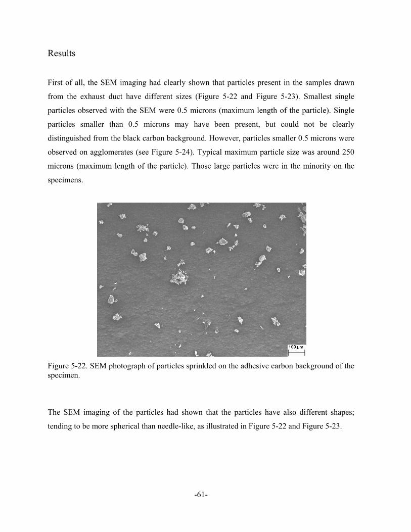
Results
First of all, the SEM imaging had clearly shown that particles present in the samples drawn
from the exhaust duct have different sizes (Figure 5-22 and Figure 5-23). Smallest single
particles observed with the SEM were 0.5 microns (maximum length of the particle). Single
particles smaller than 0.5 microns may have been present, but could not be clearly
distinguished from the black carbon background. However, particles smaller 0.5 microns were
observed on agglomerates (see Figure 5-24). Typical maximum particle size was around 250
microns (maximum length of the particle). Those large particles were in the minority on the
specimens.
Figure 5-22. SEM photograph of particles sprinkled on the adhesive carbon background of the specimen.
The SEM imaging of the particles had shown that the particles have also different shapes;
tending to be more spherical than needle-like, as illustrated in Figure 5-22 and Figure 5-23.
-61-

Figure 5-23. SEM photograph of typical dust particles.
Higher magnification images (magnification > 1500) also revealed that particles of different
and equal size had often formed agglomerates (Figure 5-24). These agglomerates could have
been formed during the smelting process in the cells, during the transport of the exhaust gas
through the duct system, in the isokinetic sampling apparatus (especially in the cyclone),
during the transport of the sample bottle from the smelter to the laboratory or due to the
preparation method of the specimen. However, all these described steps, which the dust
particles go through before being examined with laboratory equipment, may also lead to the
event that particles and agglomerates are breaking apart. This event cannot be observed with
the SEM since possible broken pieces from a particle could also be identified as a single,
independent particle.
-62-

Figure 5-24. SEM photographs of particles with different sizes; multiple smaller particles are agglomerated to the particle surfaces of the larger ones.
5.4 Particle size distribution (PSD)
The particle size distribution (PSD) is by definition “a description of the size and frequency of
particles in a population” whereby a particle is defined as “a discrete element of material
regardless of its size” (Jillavenkatesa et al. 2001).
-63-

The evaluation of the PSD in the present study can help understanding the fouling process on
heat exchanger surfaces exposed to the exhaust gas stream coming from the aluminum
reduction cells (see chapter 6.1 for further details). The PSD is typically expressed in a
number, volume or mass distribution, dependent on the application and/or the analysis method
used.
5.4.1 Laser Diffraction Meter (LDM)
Particle size distribution of powders can be determined using numerous commercially
available instruments, or using instruments designed for operations in very specific
environments. For a wide range of industries laser diffraction has become the preferred choice.
A Laser Diffraction Meter (LDM) can be used for the non-destructive analysis of wet or dry
samples, with particles in the size range 0.02 to 2.000 microns and has inherent advantages
that make it preferable to other options for many different materials. (Jillavenkatesa et al.
2001; Kippax 2005). For this reasons it was decided to conduct the PSD by using laser
diffraction. Thus, particles were sampled at the aluminum smelter such that the drawn dust
samples could be analyzed in the laboratory with the LDM (see chapter 5.1).
A Laser Diffraction Meter (LDM) of type Sympatec Helos was used to identify PSD of the
dust in front of the dry scrubber. The Icelandic Innovation Center (NMI) provided the LDM
and assisted the analysis process. The instrument is capable for being connected with a dry or
wet powder disperser. The latter one, of type Sympatec SUCELL (Figure 5-26), was used in
this study since wet powder dispersion requires smaller sample quantities (≈ 0.05 g) for
conducting several measurements than the dry method.
The LDM relies on the principle that particles passing through a laser beam will scatter light at
an angle and intensity that is directly related to their size. As demonstrated in Figure 5-25,
large particles scatter light at narrow angles with high intensity, whereas small particles scatter
at wider angles, but with low intensity (Kippax 2005). The diffraction patterns are detected by
-64-

sensors and compared to an appropriate optical model for determining the particle size
distribution. Traditionally, two different models are used, the Fraunhofer Theory and the Mie
Theory (Kippax, 2005). The instrument at NMI evaluates the scattered patterns detected by the
sensors with the Fraunhofer Theory. The output of the particle sizes by the LDM software are
given in equivalent diameter assuming that the particles are spherical. Thus all three
dimensions (length, width, height) of a particle are automatically defined.
The measuring range of the instrument at NMI is 1.8-350 µm. The particles which are within
this measuring range are detected with an efficiency of almost 100%. Particles outside the
range may be captured by the LDM detectors, but with a smaller efficiency. The results are
output as a cumulative and density distribution in tabular and graphical (see Figure 5-27)
form.
Figure 5-25. Light scattering patterns for different particle sizes; left pattern represents a large particle which scatters the light at a narrow angle with a high intensity. The right pattern shows a small particle which scatters the light at wider angles, but with low intensity.
The particle samples (≈ 0.05 g) were added untreated to the Sympatec SUCELL disperser,
which contained de-ionized water. Added particles were dispersed by two stirrers before
passing the laser beam in a closed loop. Ultrasonication was used to check for degree of
agglomeration. Ultrasonication generates, by use of high-intensity acoustic energy, alternating
low-pressure and high-pressure waves in liquids, leading to the formation of high speed
impinging liquid jets and strong hydrodynamic shear-forces (Wikipedia contributors 2009a).
Several reading points with and without ultrasonication were taken from the circulating
particle-water stream on different samples. Ultrasonication did not have a significant effect on
the particle size distributions.
-65-

Figure 5-26. Left: Front view of the Laser Diffraction Meter (Sympatec Helos) connected to the wet disperser of type Sympatec SUCELL; right: top view of the instrument - in the photograph center the wet disperser filled with de-ionized water and with running stirrers is visible. Results
As shown in Figure 5-27, four measurements on the same dust sample were conducted with
the LDM. Before the four measurement points were taken, the stirred water-particle mixture
was ultrasonicated for a period of 120 s. Measurement no. 4 (labeled as isokinetic 4 in the
graph) was taken after an additional 120 s ultrasonication. The graphical illustration in Figure
5-27 represents the volume particle size distribution of the dust in two probability curves - the
cumulative distribution curve and the Gaussian distribution curve (bell-shape curve).
The first curve shows the cumulative volume distribution in % (left y-axis) dependent on the
particle size in µm (x-axis). E.g. if the y-value is 70% then the correlated x-value is the
particle size where all particles with smaller (or similar) equivalent diameter make up 70% of
the total detected sample volume. Whereby consequently 30% of the total detected sample
volume consists of particles with greater (or similar) equivalent diameter.
The second curve illustrates the volume density distribution (right y-axis) dependent on the
particle size in µm (x-axis). The Gaussian distribution peak represents the most frequently
occurring size (by volume) of the particles detected by the LDM; in other words, the peak is
-66-

the particle size where most of the sample’s volume is concentrated. If one would perform a
number PSD on the same sample then the Gaussian distribution peak would consequently be
at a much finer particle size (by assuming that all particles are spherical).
Figure 5-27. Particle size distribution of the particles drawn with the isokinetic sampling apparatus in front of the dry scrubber, determined with the LDM.
As shown in Figure 5-27, the modal particle size of the dust particles was 19.5 μm (by
volume) and the median particle size by volume was 18.5 μm. 95% of the total detected
sample volume were particles with equivalent diameter below 85 μm, and 50% below 18.5
μm. If the particles are assumed to be spherical and uniform density, dust particles with
equivalent diameters between 4.5 to 61 μm represent 80% of the total mass; particle sizes
below 2 μm count for 4% of the total mass.
Naess et al. (2006) found for analogous sampling in a Norwegian smelter, using a cascade
impactor, a much larger proportion of particles in the submicron range (70% by mass).
However in the present case the submicron filters downstream of the cyclone only collected
20-30% of the total collected mass (see chapter 5.1), and LDA of particles collected on the
fouling probe also indicated larger modal particle sizes (see chapter 6.2.3). The discrepancy
-67-

-68-
may be due to different pot operation, or possibly degree of agglomeration, sampling location,
or analysis methods.

6 Particulate deposition on surfaces in the exhaust gas
In the previous chapter the free-stream particles present in the exhaust gas were examined and
characterized. In the case of HX installation in these gas streams, the presence of the solid
matter may lead to significant formation of deposits on the heat transfer surfaces (fouling);
whereby the characteristics of these deposits may vary from those of the free-stream particles.
Fouling would lead to a decrease in overall heat transfer coefficient, an increase in pressure
drop, and may accelerate material corrosion.
To investigate the properties of the deposits and the fouling propensity of the exhaust gas, a
fouling probe was installed in the duct in front of the dry scrubber. Fouling build-up was
collected and analyzed for chemical composition, degree of agglomeration, and particle size
distribution using the techniques described in the previous chapter. Results are presented in
this section by comparing them to those obtained from the sampled free-stream particles and
dust samples from the Ardal aluminum smelter, Norway. The time dependent development of
the overall heat transfer coefficient, obtained from heat flux measurements with the fouling
probe, is presented in chapter 6.2.5.
6.1 The fouling process
Fouling is generally defined as the undesired deposition of material on surfaces (Epstein,
1981). Fouling can be classified according to mechanism (e.g. precipitation, chemical reaction,
particulate), process type (e.g. combustion, smelting) or by industry (e.g. cement, aluminum).
Fouling in the present study can be classified as the so called gas-side fouling, whereby
specifically particle fouling (deposition built up on surfaces) and inorganic fouling (scaling
built up on surfaces) are occurring (Temu 1998; Flemming et. al [date unknown]).
-69-

Usually four steps lead to a durable deposition of material on heat transfer surfaces (Temu,
1998):
Transport of deposits to the surface
Attachment of the deposits to the surface (deposition)
Removal of parts of the deposits from the surface (re-entrainment)
Ageing
The first step of fouling is the transport of particulate by the carrier fluid to the surface. The
transportation process depends on the dynamics of the carrier fluid, whereby the transport to
the surface is mainly controlled by diffusion (small particles), combination of inertia and
diffusion (predominately medium sized particles), and interception and inertial impaction
(predominately large particles). The transportation process may be enhanced by
thermophoresis (temperature gradients), in particular for smaller particles (Temu 1998; Naess
et. al 2006). Particle diffusion is the collision of particles with the solvent molecules (here: the
exhaust gas). The collision creates a thermal motion which may move the particles to a region
of higher or lower concentration; particle diffusion affects mostly small particles. Inertial
impaction is the strike of a particle on a surface, due to it’s sufficient inertia. Interception is
the touch of inertia-less particles to a surface; because inertia-less particles follow the
streamlines, it is more likely that large particles touch the surface. For example for a cylinder
in cross-flow, deposition of submicron particles can occur due to inertial impaction,
interception and diffusion; but in pipe flow the deposition of the same particles can only occur
due to diffusion (Temu 1998). This may explain the results obtained from pilot tests by
Sorhuss and Wedde (2009), where less fouling had been built up by using a counter flow
vertical HX containing pipes with water on the outside and exhaust gas on the inside (see
chapter 2.3).
If a particle reaches the surface it either deposits since it adheres, or slides along the surface
and then adheres (deposition), or it is re-entrained to the flowing fluid since it slides along the
surface without adhering, or it directly bounces off (Naess et. al 2006).
-70-

Since fouling is a dynamic process, a certain amount of material may be removed from the
surface and is re-entrained in the flowing stream. This effect is influenced by a number of
forces. There are on the one hand forces which adhere the particles to the surface (e.g.
electrostatic, thermophoretic, surface tension, gravitational forces) and on the other hand
forces that counteract the adhesion forces (e.g. shear and lift forces of the flowing gas,
impaction of larger particles, gravity) (Temu 1998; Naess et. al 2006).
With time, the adhesion of deposited particles may increase, due to e.g. gradual increase in
contact area in which the attractive forces act, change in the deposit’s crystal structure and
developing of thermal stresses. The surface deposit may hardens (Temu 1998).
It can be concluded that the free-stream particles properties influence beside other forces the
fouling process; whereby the particles which deposit on the heat transfer surfaces determine
the effective thermal conductivity of the fouling layer.
6.2 Experimental set up A Fouling probe was used to examine and evaluate fouling built up on tubing in cross-flow
direction. The unit was specifically designed and built for the duct conditions at Nordural by
Hákonarson (2009). The fouling probe is capable of gathering particle deposits for analysis in
situ and in the laboratory, and is also capable of monitoring the heat flux during sampling
runs.
The cylindrical fouling probe (63 mm outer diameter) is made out of 304 stainless steel and
has a total length of 700 mm (Figure 6-1). A shield of 300 mm length and 88.9 mm outer
diameter is positioned on the 63 mm tube by using a loose bearing; whereby the radial spacing
is fixed and the inner cylinder can be retracted. Thus, an area of 300 mm on the fouling probe
tube can be protected from re-entrainment of solid matter when retracting the unit after
completed sampling runs (see Figure 6-3) (Hákonarson 2009).
-71-

Figure 6-1. The designer and constructor standing on the platform in front of the dry scrubber with his fouling probe; the 63 mm tube is in both pictures retracted from the shield (Hákonarson 2009).
The 63 mm tube can be retracted, while the shield stands in fixed position. This function is
enabled by the use of two flanges (Figure 6-1, right), whereby the one welded to the 63 mm
tube is loosened and retracted while another flange connected to the shield is fixed in placed.
During operation both blind flanges are bolted together to the access flange to ensure a fixed,
stable and non-vibrating operation in the duct (Hákonarson, 2009).
Beside the visual observation and collection of fouling deposits, the time dependent
development of the heat flux through the probe’s wall and fouling layer can be monitored with
the fouling probe. For this purpose, the probe is cooled from the inside with pressurized air
and relies on a set of HFS-4 Omega heat flux meters and thermocouples fixed on the unit, as
an adaptation of a design originally used by Temu et al. (2002). The fouling probe was
installed into the duct by Hákonarson (2009) for heat flux measurements in May and June
2009. Duration of the runs were as long as 11 days. Obtained results are presented in chapter
6.2.5.
For visual observation and collection of fouling deposits the fouling probe was installed into
the duct for runs as long as 7 days in August-October 2009. The method used for collecting
-72-

particle deposits and results obtained from in situ observations are described and presented in
the next section.
Particulate deposition
The fouling probe was installed in cross-flow direction into the duct for run durations of 6-7
days in August-October 2009. After retraction of the probe the unit was examined in situ on an
examination table positioned next to the duct on the access platform (Figure 6-2).
Visual observation after non-cooled and cooled runs showed that notable deposits had been
formed on the downstream and upstream side of the cylinder. The top and bottom of the probe
had very few or no deposits. Differences between fouling built up during cooled or non-cooled
runs were not notable by visual observation.
Figure 6-2. Fouling probe after sampling run in a fixed position on the examination table in front of the duct; the probe’s downstream side faces to the viewer; deposits from the side of interest had been already scraped off.
Deposits on the downstream side were loose and fluffy and could be easily removed by
vibration or light scraping. The deposits on the downstream side were collected with a scraper
from the area of the probe which was protected by the shield during retraction. Figure 6-3
-73-

shows the downstream side of the probe before and after scraping the particles into collection
containers. The thickness of the downstream deposits were in average around 1.5-2 mm after
runs of 6-7 days.
Figure 6-3. Side of interest on the fouling probe before (top) and after (bottom) collecting the fluffy particle deposits from the downstream side.
The deposits on the upstream side of the fouling probe formed a hard scale layer (see SEM
image in Figure 6-8 and Figure 6-9, chapter 6.2.2) that could not be removed by light scraping.
Some small flakes of a few millimeters length were loose after the unit had been cooled for
around 30-60 min at the ambient air. The flakes could be then removed in situ using tweezers
and were collected in collection containers and on adhesive SEM specimen substrates. Large
areas of the hard scale upstream deposits did not get loose and could only be completely
removed using a grinder. A solid deposit like this would of course not be desirable in a heat
exchanger, but the fouling probe was not optimized to minimize fouling for the local
-74-

conditions where it was used. The thickness of the upstream deposits were on average between
0.07 and 0.15 mm after runs of 6-7 days.
Collected downstream and upstream deposits were analyzed for chemical and physical
properties using the techniques described in the previous section. Results presented in the
following sections are obtained from samples taken from a 7 days non-cooled run in August
2009 and a 6 days cooled run in October 2009.
Dust samples collected downstream from HAL 300 smelter cells in Ardal, Norway were also
analyzed in the same way. The Norway samples were drawn by Norsk Hydro with a sampling
apparatus collecting dust on filters. For comparison, the results obtained from the dust samples
from Ardal, Norway and from the previously examined free-stream particles (see chapter 5)
are also presented in the following sections.
6.2.1 Chemical analysis
As for the free-stream samples, chemical analysis of the downstream and upstream samples
were performed using EDS, XRD and MEA. The elemental composition of the deposits
collected from the probe after a non-cooled and cooled run are listed in Table 6-1, along with
the results of the free-stream particles sampled isokinetically at the same location. The dust
samples from Ardal, Norway were analyzed with the EDS in the same way and are also listed
in Table 6-1.
As mentioned in chapter 5.2.1, the results obtained with the EDS should be used for
qualitative comparison between elements and samples rather than for firm quantitative
analysis. Differences between elemental compositions of the non-cooled and cooled deposits
are partly notable, but not significant. Deviations between these samples do not necessarily
have to be present due to stronger thermophoresis (temperature gradient) forces; they might
also be related to variations in pot operation at Nordural.
-75-

Table 6-1. Elemental composition of isokinetically sampled particles, deposited particles collected down- and upstream of the fouling probe (non-cooled and cooled), and dust samples from Ardal, Norway.
Element Isokinetic sample [weight %]
Downstreamsample (non‐cooled) [weight %]
Downstreamsample (cooled) [weight %]
Upstreamsample (non‐cooled) [weight %]
Upstream sample (cooled) [weight %]
Norwaysample [weight %]
C 37.3 25.2 27.3 2.9 3.0 15.5O 23.9 20.7 19.9 22.2 22.5 20.7F 16.5 24.9 23.8 29.1 27.5 22.1Na 5.4 9.3 9.7 16.2 16.7 20.5Al 15.1 17.3 16.7 28.0 28.1 17.5S 0.5 0.5 0.6 0.5 0.9 2.7K 0.1 0.1 0.1 0.2 0.2 0.4Ca 0.2 0.6 0.5 0.7 0.6 0.2Fe 0.5 0.6 0.6 0.3 0.3 0.0Ni 0.5 0.7 0.8 0.0 0.2 0.5Total 100.0 100.0 100.0 100.0 100.0 100.0
Conspicuous is the considerably high amount of carbon (C) present in the isokinetic and the
downstream samples, whereas the Norway and in particular the upstream samples have
significantly smaller amounts. The Norway and the upstream samples exhibit significant more
sodium (Na) then the other two samples. Aluminum (Al) is present in considerable amounts in
all samples, but is significantly higher in the upstream sample. The Norway sample has a
considerably higher amount of sulfur (S) than the Nordural samples, which is probably due to
different anodes used at the two smelters.
The XRD was used to identify the different crystalline phases. The results for the XRD
analysis are shown in Figure 6-4, with upstream and downstream samples, which were
collected from the cooled fouling probe, compared to the isokinetically sampled particles. All
three Nordural samples show very similar crystalline patterns and therefore it can be
concluded that the same phases are present. Notable variations in composition are evaluated in
Table 6-2. In addition to the samples taken at the duct in front of the dry scrubber at Nordural,
dust samples from Ardal, Norway were analyzed with the XRD. The Norway sample shows
very similar crystalline patterns to all three Nordural samples as depicted in Figure 6-4.
-76-

Figure 6-4. XRD analysis of the isokinetic, downstream and upstream (cooled) samples, and Norway sample. The phases labeled are given in Table 6-2. The patterns are raised/lowered: upstream pattern lowered by 65 counts, downstream pattern raised by 125 counts, isokinetic pattern raised by 500 counts, and the Norway pattern is raised by 750 counts.
Lin
(Cou
nts)
0
100
200
300
400
500
600
700
800
900
1000
1100
1200
1300
1400
1500
2-Theta - Scale4 10 20 30 40 50 60 7
upstream
NaAlKog
FluCryCry
ChiChi
AluAlu
Norway#1
Alu
NaAl
ChiCry
AluAluAlu
Chi
downstream
isokinetic
Table 6-2. Comparison of isokinetic samples and deposited particles down- and upstream of the cooled fouling probe. Qualitative comparisons are for the same phases between samples. Abbreviations correspond to labels in Figure 6-4.
Isokinetic sample
Downstreamsample (cooled)
Upstream sample (cooled)
Alumina (Al2O3) [Alu] less abundant medium abundance most abundant Chiolite (Na5Al3F14) [Chi]
almost absent slightly less abundant than in upstr. sample
most abundant
Cryolite (Na3AlF6) [Cry]
slightly less abundant than in downstr. sample
most abundant slightly less abundant than in downstr. sample
Kogarkoite (Na3(SO4)F) [Kog]
slightly less abundant than in downstr. sample
most abundant not notable
Fluorite (CaF2) [Flu]
slightly less abundant than in downstr. sample
most abundant almost absent
Sodium alu. fluoride (NaAlF4) [NaAl]
slightly less abundant than in downstr. sample
most abundant almost absent
Amorphous material most abundant medium abundance less abundant
-77-

The MEA was used to identify the carbon share in the downstream and upstream samples
(cooled and non-cooled) with greater accuracy (0.5%). Results are given in Table 6-3.
Isokinetically sampled particles collected with the cyclone and downstream filters on 14
August ’09 were analyzed together with this method. Particles lifted from filters used for dust
concentration measurements on 30 Sept. ‘09 were analyzed with the MEA for detecting the
carbon weight share. Both obtained results enable a more valuable comparison with the dust
sample from Ardal, Norway, which were collected in a similar way on filters from exhaust gas
from HAL 300 cells.
Table 6-3. Percentage share of carbon in the dust samples identified with the Macro Elemental Analyzer (MEA).
Sample C [weight %]Isokinetic (14.08.09)(only cyclone particles)
15.70
Isokinetic, total (14.08.09)(cyclone particles + filter particles)
11.80
Isokinetic, total (30.09.09)(filters from dust conc. measur.)
9.42
Downstream (non‐cooled) 9.92Upstream (non‐cooled) 1.04Downstream (cooled) 12.1Upstream (cooled) 0.76Norway 8.95
The results show that the share of carbon in the total isokinetic samples is around 0.5-2%
higher than in the dust sample from Norway. This is not an unexpected result since Nordural
had experienced anode problems during the sampling period of May to September 2009, as
described earlier. However, the deposits on the upstream side of the fouling probe had very
low carbon content in comparison to the other samples from Norway and Nordural.
The difference between the carbon (C) share of the non-cooled and cooled downstream
deposits is significant with around 2%. As mentioned before this cannot necessarily be
attributed to stronger thermophoresis (temperature gradient) forces, as the deposition
happened during different periods that may have been characterized by different cell
operation, but it arouses more and more the interest to set up a laboratory testing facility,
-78-

which can provide stable conditions, regarding flow velocity and distribution, and dust
concentration. Results obtained from the cooled and non-cooled fouling probe installed to this
testing facility could give worthwhile information about the influence of thermophoresis
forces on the fouling process in these gas streams.
6.2.2 Visual and microscopic observation
In situ, visual observation of the downstream deposits collected in a transparent 50 ml
container were performed. Slow rolling and rotating of the cylindrical container gave the first
impression that the deposits were more sticky and more adhesive than the one of the free-
stream particles. For further observations of the downstream deposit, the SEM was used to
obtain highly magnified 3-D images. While preparing the SEM specimens by sprinkling small
quantities of the downstream deposit on an adhesive carbon background, the first impression
of a very sticky, adhesive bulk was strengthened. It was difficult and almost impossible to
sparsely distribute the deposited particles on the specimen.
Figure 6-5. SEM image of downstream deposit taken with 220 times magnification; fine and medium sized particles had built accumulations and agglomerates.
SEM images with magnification (X) higher than 200 revealed that the majority of the fine and
medium sized particles had built either accumulations or agglomerates (Figure 6-5). Particles
-79-
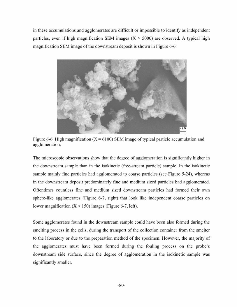
in these accumulations and agglomerates are difficult or impossible to identify as independent
particles, even if high magnification SEM images (X > 5000) are observed. A typical high
magnification SEM image of the downstream deposit is shown in Figure 6-6.
Figure 6-6. High magnification (X = 6100) SEM image of typical particle accumulation and agglomeration.
The microscopic observations show that the degree of agglomeration is significantly higher in
the downstream sample than in the isokinetic (free-stream particle) sample. In the isokinetic
sample mainly fine particles had agglomerated to coarse particles (see Figure 5-24), whereas
in the downstream deposit predominately fine and medium sized particles had agglomerated.
Oftentimes countless fine and medium sized downstream particles had formed their own
sphere-like agglomerates (Figure 6-7, right) that look like independent coarse particles on
lower magnification (X < 150) images (Figure 6-7, left).
Some agglomerates found in the downstream sample could have been also formed during the
smelting process in the cells, during the transport of the collection container from the smelter
to the laboratory or due to the preparation method of the specimen. However, the majority of
the agglomerates must have been formed during the fouling process on the probe’s
downstream side surface, since the degree of agglomeration in the isokinetic sample was
significantly smaller.
-80-
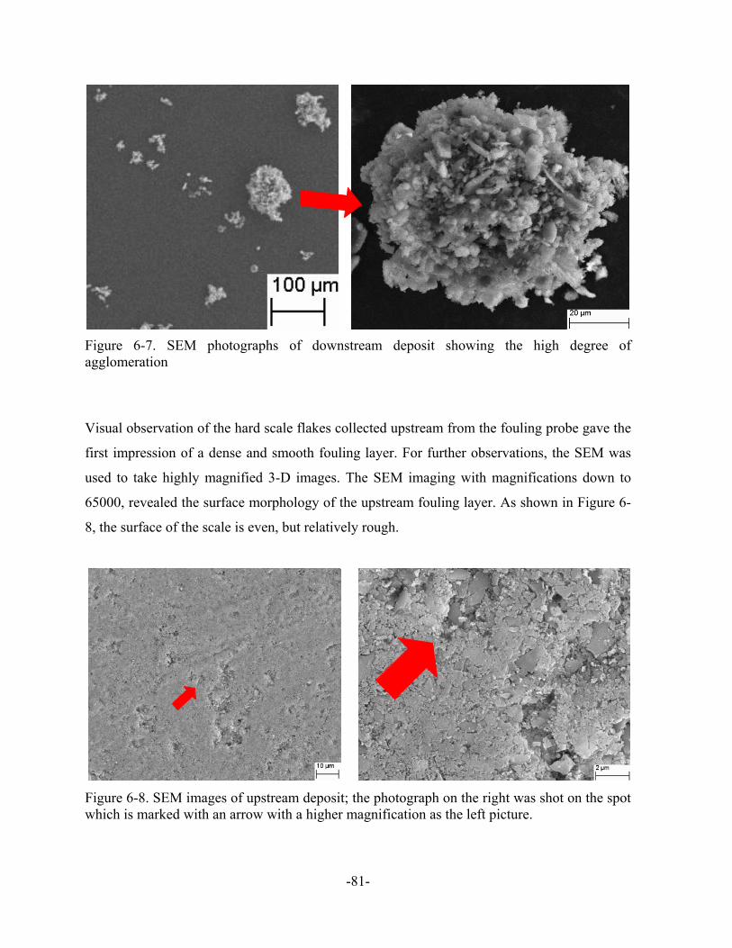
Figure 6-7. SEM photographs of downstream deposit showing the high degree of agglomeration
Visual observation of the hard scale flakes collected upstream from the fouling probe gave the
first impression of a dense and smooth fouling layer. For further observations, the SEM was
used to take highly magnified 3-D images. The SEM imaging with magnifications down to
65000, revealed the surface morphology of the upstream fouling layer. As shown in Figure 6-
8, the surface of the scale is even, but relatively rough.
Figure 6-8. SEM images of upstream deposit; the photograph on the right was shot on the spot which is marked with an arrow with a higher magnification as the left picture.
-81-
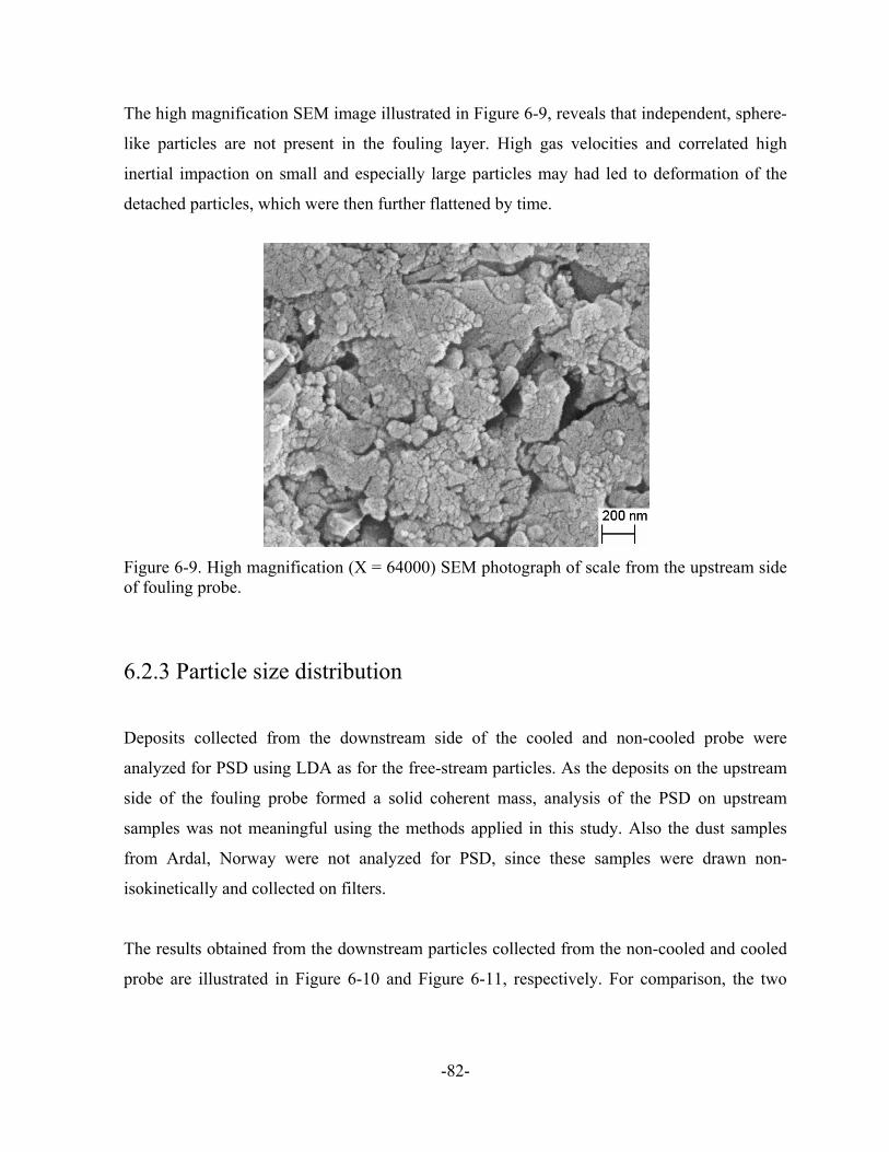
The high magnification SEM image illustrated in Figure 6-9, reveals that independent, sphere-
like particles are not present in the fouling layer. High gas velocities and correlated high
inertial impaction on small and especially large particles may had led to deformation of the
detached particles, which were then further flattened by time.
Figure 6-9. High magnification (X = 64000) SEM photograph of scale from the upstream side of fouling probe.
6.2.3 Particle size distribution
Deposits collected from the downstream side of the cooled and non-cooled probe were
analyzed for PSD using LDA as for the free-stream particles. As the deposits on the upstream
side of the fouling probe formed a solid coherent mass, analysis of the PSD on upstream
samples was not meaningful using the methods applied in this study. Also the dust samples
from Ardal, Norway were not analyzed for PSD, since these samples were drawn non-
isokinetically and collected on filters.
The results obtained from the downstream particles collected from the non-cooled and cooled
probe are illustrated in Figure 6-10 and Figure 6-11, respectively. For comparison, the two
-82-

PSD probability curves of the free-stream (isokinetic sampled) particles are also shown in
Figure 6-10.
The PSD of the downstream particles, which were collected from the non-cooled probe,
indicated a modal particle size of 9 μm (in equivalent diameter), which is much less than the
modal particle size for the isokinetic samples. If the particles are assumed to be spherical and
uniform density, dust particles larger than 2.1 μm represent 90% of the total mass.
Figure 6-10. PSD of particles collected from the downstream side of the fouling probe and isokinetically sampled particles; the fouling deposits were collected from the unit after it ran for 7 days non-cooled in the duct.
isokineticdownstream
The PSD of the downstream particles, which were collected from the cooled fouling probe, is
almost similar to the one obtained from the non-cooled probe. The indicated modal particle
size is 10 μm, whereby it is 9 μm in the previous case. Only significant deviations between
both downstream samples is the share of larger deposited particles. In the cooled-case (Figure
6-11) 5% of the total detected sample volume consists of particles larger than 30 μm, whereby
in the non-cooled case the share is only 1%. Due to these deviations, an implementation of a
testing facility for examining thermophoresis influences might be worthwhile, as discussed
earlier.
-83-

Figure 6-11. PSD of particles collected from the downstream side of the fouling probe; the unit was running for 6 days in the duct, while it was cooled from the inside.
Figure 6-12. PSD of particles collected from the downstream side of the cooled fouling probe, determined with the LDM using the dry disperser (RODOS) instead of wet disperser (SUCELL).
Since larger quantities could be collected from the downstream side of the probe than with the
Isokinetic Particle Sampler, an additional dry analysis was performed with the LDM
(Sympatec Helos) using a dry disperser (RODOS). In this apparatus, particles are dispersed by
-84-

passing them over a high frequent vibrating plate. The dust is then accelerated in an air stream
and led through the laser beam of the LDM before it is sucked into an exhaust system. The
results from the dry analysis are slightly different to those obtained from the wet analysis,
whereby the PSD of the dry sample is notable finer. The modal particle size is 7.3 μm and
34% of the total volume is below a particle size of 2 μm; whereby in the wet analysis modal
particle size is 10 μm and only 22% of the total volume is below a particle size of 2 μm.
In general, the experimentally obtained results from the exhaust gas at Nordural agree with the
theoretical basics of the fouling process described in chapter 6.1. Larger particles, due to their
inertia, penetrate through the boundary layer and may be collected at the front, whereby
mainly finer particles (< 60-80 μm) deposit at the back since they follow the stream lines and
are caught in the wake after flow separation. The larger share of carbon in the downstream
sample may indicate that the carbon is more predominant as finer particles. This should be
researched further by e.g. performing element mapping.
6.2.4 Surface corrosion and dew point
Gases occurring in the exhaust gas, such as CO2 and SO2 (see chapter 4.1), are non-corrosive
to metals and alloys if they are in a dry environment with moderate temperatures. If liquid
water or aqueous solutions are present than these gases form acids, such as carbonic and
sulfuric acid, which become quite corrosive (Þórarinsdóttir 2009).
After test runs with the cooled fouling probe, pitting occurred on the surface upstream and
downstream of the cylindrical tube (304 stainless steel). This indicates that the surface
temperature of approximately 50°C may have been below the acid dew point for the exhaust
gas. This should be researched further.
-85-

-86-
6.2.5 Heat flux measurements
Heat flux measurements were performed at the duct in front of the dry scrubber by
Hákonarson (2009). The fouling probe was installed in cross-flow direction for test runs in
May and June 2009. Over a period of 11 days the overall heat transfer coefficient was
observed to drop by 3% on the upstream side and by 29% on the downstream side, while the
probe was cooled from the inside with compressed air at ambient temperature. More than half
of the decrease in the overall heat transfer coefficient on the downstream side occurred in the
initial two days. Heat flux on surfaces parallel to the flow was not measured, which is
reasonable since no or little fouling had built up on these areas. It may be assumed that the
heat flux did not decrease on the top and bottom of the fouling probe, which would result in an
overall heat transfer coefficient drop (for the probe as a whole) of around 7% over a 11 day
period.

7 Heat recovery potential of the exhaust gas
7.1 Thermal energy content
In 2008 the average duct temperature in front of all four FTPs at Nordural was 73°C. Due to
the pot sealing program finished in spring 2009 a 2-3°C higher exhaust gas temperature can be
expected under the current smelter configurations (See chapter 3.2.1). This results
consequently in an annual average duct temperature of 75.5°C. As mentioned in chapter 3.2.2,
a significant decrease of the exhaust gas flow rate due to the pot sealing program was not
observed. The average flow rate per cell in 2008 in potline 1 and 2 at Nordural was 1.75 Nm³/s
which results in a massflow of 2.1 kg/s per cell by assuming a normal density of 1.2 kg/Nm³
for the exhaust gas. The total average flow rate and mass flow of the exhaust gas from all 520
prebake cells is therefore 912 Nm³/s and 1094 kg/s, respectively. The thermal energy content
of the exhaust gas at Nordural can be determined with following general known
thermodynamic equation:
gas gas p,gas gas,in ref Q m c T ‐T(⋅ ⋅& & (7-1)
whereby Qgas is the thermal energy content of the exhaust gas, mgas the mass flow of the
exhaust gas, cp,gas the heat capacity of the exhaust gas, Tgas,in the duct temperature and Tref the
reference temperature.
As reference temperature, the annual mean temperature in Iceland, 5°C, is used (Wikipedia
contributors 2009c). By using the heat capacity of dry air under normal conditions (1 kJ/kg)
for the exhaust gas the total average thermal energy that could be extracted from the exhaust
gas in front of all FTPs at Nordural is 77.1 MWth. In practice the exhaust gas has a humidity
close to that of ambient air due to the false air dilution. Condensation of the water vapor would
increase the thermal efficiency of the HX due to released latent heat, but may not be desirable
because of simultaneously induced acid corrosion (see chapter 6.2.4).
-87-

A total average energy content of 77.1 MWth promises a huge potential which may be
attractive to harness if one regards the fact that around 8,000 liters per hour of no.2 heating oil
have to be burnt in a domestic boiler having a 88% conversion efficiency to release a similar
amount of heat (Tester et al. 2005). Ambient temperatures in Iceland are cool but relatively
constant due to the maritime climate; with mean temperatures around 0°C in winter and 10°C
in summer (Wikipedia contributors 2009c). At other smelters with higher cell currents and
tighter pots, exhaust gas temperatures are generally higher. Thus, the exhaust gas from these
smelters has probably an even higher total energy content and therefore a higher heat recovery
potential. The total energy potential for exhaust gas with temperatures differences Tgas,in - Tref
= 70 to 130 K and a mass flow of 2.1 kg/s per cell is listed in Table 7-1.
Table 7-1. Thermal energy content of exhaust gas from aluminum reduction cells for gas temperature differences between 70 and 130 K; based on mass flow of 2.1 kg/s per cell.
Temp. difference (T_gas,in ‐ T_ref)
[K]
Energy content per cell [MWth]
Energy content of 520 cells
[MWth]70 0.147 76.690 0.189 98.5110 0.231 120.3130 0.274 142.2
From a practical point of view the heat recovery from the exhaust gas of aluminum reduction
cells has certain constraints, especially in regard to electricity generation, due to the relatively
low gas temperatures of around 70-150°C.
The practical heat recovery potential is determined in the following chapters by considering
different low temperature applications, such as space and district heating and electricity
generation with a binary system.
-88-

7.2 Utilization opportunities
In chapter 2.3 it was described that recovering heat from the exhaust gas upstream of the dry
scrubber may have alone an economical benefit due to reduction in fan power consumption, if
pressure drops across the HX are kept to be low. Lowering of the temperature upstream of the
dry scrubber may lead also to an extension of the filter-bags life.
There are two ways of harnessing the heat which is recovered with a HX system from the
exhaust gas: direct use and indirect use. Direct use consists of all types of utilization except
power generation. In general direct use applications harness the resource more efficiently than
power generation systems as no energy is lost due to conversion of heat into electricity.
However, heat cannot be transmitted over distances of more than some kilometers at most
without a notable reduction of efficiency due to inevitable heat losses.
Figure 7-1. Lindal-diagram, showing possible utilization applications of geothermal energy at different temperatures; appropriate for water/steam coming from other sources, such as solar collectors or heavy industries processes (Ragnarsson 2008).
-89-

The Lindal-diagram (Figure 7-1) shows typical utilization of hot water/steam at different
temperatures. Most commonly used applications for (geothermal) hot water/steam in Iceland
are space heating (59.5%), power generation (20.2%), fish farming (5.8%), swimming pools
(4.4%), snow melting (4.4%), greenhouses (3%) and industrial process heat (2.7%)
(Ragnarsson, 2008). In the following chapters the most common and promising utilization
types are analyzed and evaluated.
7.2.1 Space and district heating
Space and district heating (S&DH) systems utilizing waste heat from the exhaust gas of
aluminum smelters have been commercially used for a few decades. The Norwegian local
communities around the Hydro smelters in Høyanger and Sunndaløra are utilizing the heat
recovered from the exhaust gas downstream of the dry scrubbers. The system at the Høyanger
smelter with a maximum capacity of 4.2 MWth has been in operation since 1981 and the
distribution net in Sunndalsøra started operating in 2004. The HX at the Sunndalsøra smelter
has a maximum capacity of around 6 MWth and is backed up by a 8 MWth gas boiler
(Lorentsen OA. e-mail to author. 2009 Nov 02).
Distribution of recovered heat from heavy industries has not been performed yet in Iceland,
but long experience with geothermal energy and a strong existing distribution infrastructure
make Iceland a prime location to consider the use of heat from exhaust gas for district heating
purposes. In the case of the Nordural smelter in Grundartangi, the nearby town of Akranes,
home to approximately six thousand people and several industries, is currently serviced by a
geothermal hot water pipeline from the Deildartunguhver hot spring, 62 km away (Ragnarsson
and Hrólfsson 1998). A gradual decline in the output of this spring and maintenance
difficulties make supplanting or even replacing the system potentially attractive. Ragnarsson
and Hrólfsson (1998) mention in their technical description about the district heating (DH)
system in Akranes that the tunnel under the fjord Hvalfjördur (opened in 1998) shortens the
driving distance between Reykjavik and Akranes by some 60 km. The distance between the
-90-

northernmost part of the Reykjavik DH distribution system and Akranes is now less than 20
km. Thus, it might be economical to connect these two systems through the tunnel instead of
maintaining the long transmission pipeline to Akranes. They come to this conclusion by listing
previously several disadvantages of the existing 62 km pipeline from the Deildartunguhver hot
spring to Akranes:
The pipeline was built from asbestos cement in 1979, just a short time before asbestos
was recognized as hazardous to people’s health and it was later forbidden as a pipe
material. By using asbestos pipes instead of pre-insulated steel pipes the investment
cost could drastically be reduced.
Also, though asbestos has good thermal properties it is rather fragile and the pipeline
suffers from frequent breaks. The asbestos pipe breaks down in average 20-30 times
per year. The breaks are detected automatically and repaired quickly, but with high
costs.
The flow rate in the transmission pipe is regulated to keep a constant supply
temperature of 77°C from the pumping station at Akranes. Excess flow has to be
spilled to keep the water temperature at an acceptably low level. It can vary from 80 l/s
during summer to no excess flow during winter peaks.
Earth cover of the transmission pipeline has eroded and in some places consolidated
due to drying, so the pipeline has sunken below the original ground surface level. In
attempt to solve this problem, trenches have at some places been dug on both sides of
the pipeline.
The heating cost in Akranes are among the highest of all district heating systems in
Iceland. It is, for example, about 60% above the heating cost in Reykjavik.
In the technical description by Ragnarsson and Hrólfsson (1998) a replacement of the 62 km
transmission pipeline by a pipe system carrying heat recovered from Nordural aluminum
smelter over 17 km to the town of Akranes was not considered. In Akranes the water
temperature at the inlet to the distribution system is 77°C and the average temperature to the
users is 72.5°C. The total annual hot water consumption of the town is around 1.32 million m³
-91-

(status 1998), which is used directly by the users in their radiator systems and as domestic hot
water. The return water is disposed of through the local waste water system.
The temperature inlet value of 77°C cannot be obtained with HXs applied to the exhaust ducts
in front of the FTPs under current running conditions of the Nordural smelter without any
modifications of the cells or ductwork. As mentioned in the previous chapter the annual
average exhaust gas temperature is 75.5°C, whereby it is in average 70.5°C in winter time.
However, thoroughly insulating the ductwork from the outside would lead to a significant
temperature rise. Temperature measurements performed on potline 1 at six exhaust ducts right
after the cells in March 2009 show the annual average gas temperature leaving the cells is
around 100-120°C. A gas temperature increase of perhaps 20-40°C may be obtainable in front
of the dry scrubber. Thus, a supply temperature of 77°C to the town of Akranes may be
obtainable all over the year and during the coldest winter periods - even with a reasonable
temperature difference of 10 K between the hot side (exhaust gas) and the cold side (water) of
the HX. The temperature drop in the transmission pipeline between the smelter and the
community will be small, especially during the peak winter season (< 2°C), due to high flow
rates and the use of state of the art pre-insulated steel pipes with large diameters. The
temperature drop of the 35°C return water will be less significant and is not considered in this
study. The S&DH system may be backed up by a hot water storage tank at Akranes (which is
already existing) for ensuring a hot water supply to the costumers also during maintenance
periods and unusual cold days in winter season.
With a 72.5°C supply temperature to the users, the return temperature will be around 35°C
when using the existing radiators installed in the houses and buildings at Akranes
(Gunnlaugsson E. e-mail to author. 2009 Nov 27). As described earlier in chapter 2.3 the
exhaust gas inlet temperature to the dry scrubber must be held below a maximum temperature
limit to prevent filter-bag damage and to meet emissions requirements. However, kinetics of
the fluorine reaction with alumina on the filter bags requires the temperature to also be
maintained above a lower temperature limit depending on the design. It is possible that heat
exchange may need to take place in a two-stage series process across both sides of the filters,
-92-
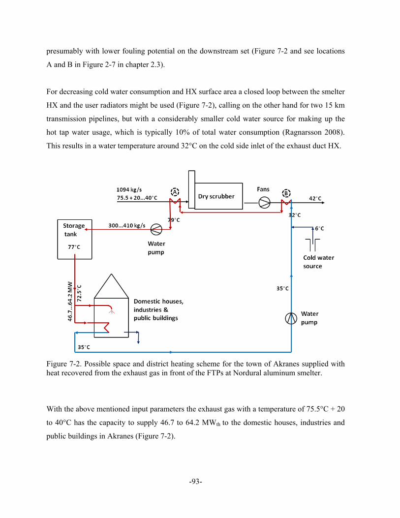
presumably with lower fouling potential on the downstream set (Figure 7-2 and see locations
A and B in Figure 2-7 in chapter 2.3).
For decreasing cold water consumption and HX surface area a closed loop between the smelter
HX and the user radiators might be used (Figure 7-2), calling on the other hand for two 15 km
transmission pipelines, but with a considerably smaller cold water source for making up the
hot tap water usage, which is typically 10% of total water consumption (Ragnarsson 2008).
This results in a water temperature around 32°C on the cold side inlet of the exhaust duct HX.
Figure 7-2. Possible space and district heating scheme for the town of Akranes supplied with heat recovered from the exhaust gas in front of the FTPs at Nordural aluminum smelter.
With the above mentioned input parameters the exhaust gas with a temperature of 75.5°C + 20
to 40°C has the capacity to supply 46.7 to 64.2 MWth to the domestic houses, industries and
public buildings in Akranes (Figure 7-2).
-93-

A typical family home of 150 m2 in Iceland has an energy consumption for heating and hot tap
water of around 30,000 kWhth/year, utilizing on average 700 m³ hot water/year (Ragnarsson
2008). Thus, the smelter exhaust gas capacity with the present S&DH set up is sufficient for
supplying 14,000 to 18,000 homes with base load by providing 300 to 410 kg/s of 79°C hot
water to the storage tank. It may be furthermore estimated that each smelter pot that consumes
0.9 MWe of electrical power could contribute towards a heating/hot water base load of a
maximum of 29 homes. By considering the presence of peak demand during the year the heat
recovered from the Nordural smelter may be sufficient for independently supplying 5000 to
7000 homes, and accordingly approximately 17,000 to 23,000 inhabitants (Ragnarsson Á. e-
mail to author. 2009 Oct 15). These numbers of homes and inhabitants are considerably higher
than the current numbers for Akranes.
However, one has to consider that the recovered heat potential may become insufficient for
independently supplying a town of a size like Akranes, if HX efficiencies go significantly
down over certain periods of time due to fouling. This applies in particular if no applicable
means to prevent fouling built up are taken and no approved cleaning procedures are applied.
The heat flux measurements with the fouling probe in chapter 6.2.5 underline this conclusion.
With present state of the art HX technology, knowledge and experience with recovering heat
upstream of the dry scrubbers it may not be recommended to set up presently a S&DH scheme
without a backup heat source, such as a geothermal hot water supply.
Nevertheless, this alternative S&DH scheme for the town of Akranes shows that aluminum
smelter exhaust gases have the potential to be harnessed for such purposes. At other smelters
with higher ambient and resultant higher exhaust gas temperatures, S&DH systems become
even more technical feasible.
Typical Icelandic district heating schemes utilize a geothermal fluid supply with 80/40/-15
radiators4, resulting in a 40°C temperature drop (Karlsson and Ragnarsson 1995). This results
in considerably larger radiators than in fuel fired European DH systems where a 90/70/-15
4 80/40/-15 radiator: 80°C inlet and 40°C outlet radiator temperature; -15°C design ambient temperature
-94-
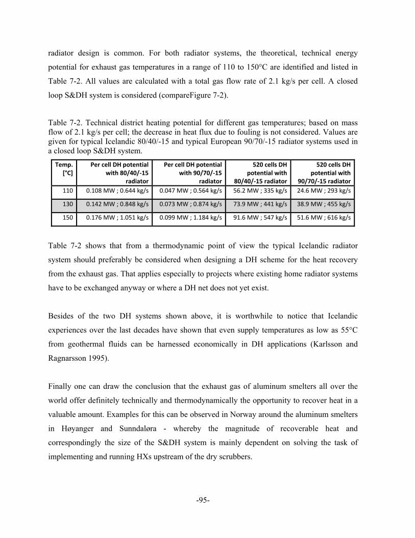
radiator design is common. For both radiator systems, the theoretical, technical energy
potential for exhaust gas temperatures in a range of 110 to 150°C are identified and listed in
Table 7-2. All values are calculated with a total gas flow rate of 2.1 kg/s per cell. A closed
loop S&DH system is considered (compareFigure 7-2).
Table 7-2. Technical district heating potential for different gas temperatures; based on mass flow of 2.1 kg/s per cell; the decrease in heat flux due to fouling is not considered. Values are given for typical Icelandic 80/40/-15 and typical European 90/70/-15 radiator systems used in a closed loop S&DH system.
Temp. [°C]
Per cell DH potential with 80/40/‐15
radiator
Per cell DH potential with 90/70/‐15
radiator
520 cells DH potential with
80/40/‐15 radiator
520 cells DH potential with
90/70/‐15 radiator110 0.108 MW ; 0.644 kg/s 0.047 MW ; 0.564 kg/s 56.2 MW ; 335 kg/s 24.6 MW ; 293 kg/s
130 0.142 MW ; 0.848 kg/s 0.073 MW ; 0.874 kg/s 73.9 MW ; 441 kg/s 38.9 MW ; 455 kg/s
150 0.176 MW ; 1.051 kg/s 0.099 MW ; 1.184 kg/s 91.6 MW ; 547 kg/s 51.6 MW ; 616 kg/s
Table 7-2 shows that from a thermodynamic point of view the typical Icelandic radiator
system should preferably be considered when designing a DH scheme for the heat recovery
from the exhaust gas. That applies especially to projects where existing home radiator systems
have to be exchanged anyway or where a DH net does not yet exist.
Besides of the two DH systems shown above, it is worthwhile to notice that Icelandic
experiences over the last decades have shown that even supply temperatures as low as 55°C
from geothermal fluids can be harnessed economically in DH applications (Karlsson and
Ragnarsson 1995).
Finally one can draw the conclusion that the exhaust gas of aluminum smelters all over the
world offer definitely technically and thermodynamically the opportunity to recover heat in a
valuable amount. Examples for this can be observed in Norway around the aluminum smelters
in Høyanger and Sunndaløra - whereby the magnitude of recoverable heat and
correspondingly the size of the S&DH system is mainly dependent on solving the task of
implementing and running HXs upstream of the dry scrubbers.
-95-

7.2.2 Electricity generation using a binary system
In the event that cell exhaust gas temperatures can be raised to 130-150°C or higher, waste
heat power generation techniques using technology such as binary cycles may become
feasible. This could be achieved by better cell sealing or more sophisticated strategies such as
the Distributed Pot Suction (DPS) system under development by Norsk Hydro as reported by
Lorentsen et al. (2009), which aims for significantly reduced suction volume with the same
hooding efficiency. Nevertheless, the first law energy conversion efficiency at these low
temperatures (130-150°C) is quite low, i.e. around 10% (Dipippo 2007), and in Iceland the
availability of low cost power from large-scale hydro and geothermal sources may make this
option uncompetitive. However, at other locations where electricity is at a higher premium,
implementation of a binary plant may be more appealing.
Typical binary systems used for low temperature applications are the Organic Rankine Cycle
(ORC) and the Kalina Cycle. Latter one is shown in Figure 7-3 in a PFD. Both power cycles
use a process fluid (e.g. Isopentane in the ORC or a mixture of ammonia-water in the Kalina
Cycle) which is heated by an external medium in one or more HXs and boils at low
temperatures, so that the generated vapor can be expanded in a turbine. The process fluid is
liquefied after the turbine by extracting heat with a cooling medium, before it is pumped to the
higher pressure level with a process pump (Fleer 2008).
Binary power cycles are commonly used for geothermal and low-temperature waste heat
applications. These technologies are available as either custom-built or modular package units
from a number of suppliers, with unit sizes ranging from < 1 to ~ 15 MWe. The adaption of the
binary vaporizer to handle exhaust gas instead of the normal hot water may be a fruitful path
for additional research.
-96-
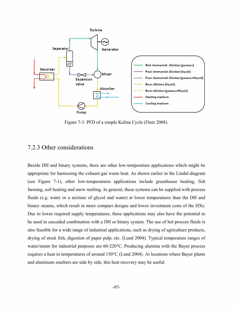
Figure 7-3. PFD of a simple Kalina Cycle (Fleer 2008).
7.2.3 Other considerations
Beside DH and binary systems, there are other low-temperature applications which might be
appropriate for harnessing the exhaust gas waste heat. As shown earlier in the Lindal-diagram
(see Figure 7-1), other low-temperatures applications include greenhouse heating, fish
farming, soil heating and snow melting. In general, these systems can be supplied with process
fluids (e.g. water or a mixture of glycol and water) at lower temperatures than the DH and
binary steams, which result in more compact designs and lower investment costs of the HXs.
Due to lower required supply temperatures, these applications may also have the potential to
be used in cascaded combination with a DH or binary system. The use of hot process fluids is
also feasible for a wide range of industrial applications, such as drying of agriculture products,
drying of stock fish, digestion of paper pulp, etc. (Lund 2004). Typical temperature ranges of
water/steam for industrial purposes are 60-220°C. Producing alumina with the Bayer process
requires a heat in temperatures of around 150°C (Lund 2004). At locations where Bayer plants
and aluminum smelters are side by side, this heat recovery may be useful.
-97-

Another option for electricity generation is the use of thermoelectric devices, in which a
temperature gradient creates a electric potential. The advantage for these systems is that no
working fluid is required. As described in chapter 2-3, a working fluid which leaks into the
reduction cells may react with the molten aluminum and cause an explosion. According to the
manufacturer CSIRO, their thermoelectric device can survive the harsh environment of
aluminum smelters and can be used to generate electricity from 150°C hot exhaust gas (Lovatt
and Wilkinson 2008), although it is likely that efficiencies would be less than for the binary
plants.
Figure 7-4. Schematic of the synergy between an aluminum smelter, a gas- and coal power plant and a CO2 scrubber plant (Lorentsen et al. 2009).
Furthermore, recovered heat from aluminum smelters could be used for supplying CO2
scrubbing plants with thermal energy. A combination of waste heat recovery and CO2 capture
is currently under development by Norsk Hydro (Lorentsen et al. 2009). Amine and chilled
ammonia used for capturing CO2 need huge quantities of heat to release the CO2 from the
adsorption media. This heat could be recovered from the aluminum smelting process (e.g.
exhaust gas, anode yokes, side walls). Since the CO2 concentrations in the exhaust gas of
modern reduction cells are low (≈ 1%), CO2 capture from these gas stream is both challenging
and expensive. One possible approach for solving this task may be the use of the earlier
mentioned Distributed Pot Suction (DPS) system to increase the CO2 concentration in the
-98-

-99-
cell’s exhaust gas. Another approach may be the conjunction of the cell’s exhaust gas with the
exhaust gas of conventional gas- and/or coal fired power plants to increase overall CO2
concentrations. The latter approach is illustrated schematically in Figure 7-4. The exhaust gas
sucked from the smelting cells contains, due to dilution air, a high share of oxygen. If purified
(cleaned) further the exhaust gas may be used in the combustion process of a gas- and/or coal
plant. The efficiency of the combustion process, due the pre-heated combustion “air”, would
be increased. Heat recovered from the aluminum smelting process (e.g. anode yokes, side
walls) may also supply the required heat to capture the CO2 from the exhaust stream coming
from the gas- and/or coal plant.

8 Conclusion
The exhaust gas with an approximately 30-45% share of the cell’s total heat loss is one of the
most valuable and most accessible heat streams in an aluminum smelter. Placement of heat
exchangers in the smelter’s courtyard, upstream or downstream of the dry scrubbers, allows
for an almost unconstrained, but compact design of these units; and the placement of the heat
exchangers upstream of the dry scrubber provides higher gas temperatures and allows for
higher thermal efficiencies. As a side benefit reduction of the gas temperature at this location
has the potential to reduce exhaust gas fan power, especially at smelters that rely on sucking in
false air upstream of the dry scrubber to protect the expensive filter bags from damage,
prolong their operation time, and meet required HF emission levels.
However, the heavy dust content of 0.26-0.38 g dust/kg exhaust gas calls for careful
antifouling provisions in the design of these heat exchangers. EDS analysis had shown that the
main elements present in the free-stream particles are carbon, oxygen, fluorine and aluminum.
Also notable amounts of sodium and some trace amounts of sulfur, potassium, calcium, iron
and nickel were found.
The free-stream particles and the deposits collected upstream and downstream of a cross-flow
mounted fouling probe appeared to have similar crystalline phases. XRD analysis conducted
that the solid matter mainly consist of alumina, followed by chiolite, cryolite and kogarkoite,
and with trace amounts of fluorite and sodium aluminum fluoride. The alumina phase
identified in the XRD was exclusively alpha, which rules out the alumina feedstock as a
source for dust particles. Also amorphous material was found with the XRD in all three
samples, and was most abundant in the free-stream particles. This was independently verified
by EDS and Macro elemental analysis, which also indicated substantial carbon. The MEA
depicted a carbon share of 15.7% in the particles which were isokinetically sampled and
collected with a cyclone. The carbon shares in the deposits collected up- and downstream of
the fouling probe were significantly lower with 0.9% and 11.0%, respectively.
-100-

Dust samples drawn from the Ardal aluminum smelter, Norway showed very similar
crystalline patterns to all three Nordural samples. However, the carbon share was significantly
lower (by 0.5 to 2%) than in the Nordural samples, which were collected from the cyclone and
the downstream filters. The higher carbon share at Nordural may be attributed to anode
problems at the smelter during the sampling periods.
Theoretical and experimental research had shown that the gas-side fouling process is strongly
related to the orientation of the heat exchanger surfaces to the stream lines. Fouling built up
rapidly (<1 week) on the in cross-flow mounted fouling probe. On the upstream side a hard,
durable scale was formed, whereas on the downstream side a thick, fluffy and low thermal
conductivity layer was built up. The top and bottom of the probe had no or only few deposits
after runs as long as one week.
Wet LDA determined a modal particle size in the isokinetic samples of 19.5 μm (by volume),
whereas the modal particle size of particles deposited on the downstream side of the fouling
probe was noticeably smaller, at 9.5 μm. In the isokinetic and downstream samples 95% of the
total detected sample volume consisted of particles smaller than 90 μm and 24.5 μm,
respectively.
For the fouling probe aligned in cross-flow direction, the reduction in overall heat transfer
coefficient was observed to drop by 3% on the upstream side and by 29% on the downstream
side in run periods as short as 11 days.
Based on observations at Nordural, the total exhaust gas flow of 912 Nm³/s at a temperature of
105°C has the potential for recovering 55 MWth, if used in a district heating scheme. This
would be sufficient to supply 16,000 homes of the nearby town Akranes with base load, by
providing around 350 kg/s of 79°C hot water to the storage tank. However, HX antifouling
provisions and proper insulation of the ductwork are essential to maintaining a maximum
thermal output. Due to a lower temperature limit upstream of the filter bags, it is possible that
heat exchange may need to take place in a two-stage series process across both sides of the dry
scrubber, presumably with lower fouling potential on the downstream set.
-101-

For the HX design, in particular for the one upstream of the dry scrubber, one should aim for a
compact unit where fouling is avoided, or at least kept to a minimum, to prevent reductions in
heat exchanger efficiency, increases in pressure drop across the heat exchanger, and expensive
maintenance. Adoption of fouling and scale removal techniques and corrosion monitoring may
be required as well.
FUTURE WORK
An important challenge for harnessing the exhaust gas heat in a wide scale, with applications
such as the district heating and binary system, is to raise the exhaust gas temperature to allow
for better thermal and first law efficiencies and more compact heat exchangers. This can be
achieved by means, such as better cell sealing or the Distributed Pot Suction (DPS). However,
it is possible that higher exhaust gas temperatures and change of the velocity profile will
introduce different types and mechanisms of fouling deposition and these influences should be
tracked closely for corresponding heat exchanger design. Results obtained from fouling
deposits collected from the fouling probe after cooled and non-cooled runs showed notable
deviations in chemical composition and particle size distribution. Due to possible variations in
the cell’s operation these deviations cannot definitely traced back to thermophoresis forces.
Setting up a laboratory testing facility, which can provide stable flow and dust conditions,
could help to better understand these effects in future.
Particle sampling was performed in this study with an isokinetic sampling apparatus,
collecting solid matter with a cyclone and downstream filters down to 0.45 µm. The cyclone
collection efficiency for the gas stream at Nordural was determined to be 70-80%. However,
some particles smaller than 0.45 microns may not have been collected. To allow for a definite
exclusion of the submicron particles being the major contributor to the total mass, a cyclone
with smaller body diameter may be used, whereby the LDM, if applied, should have a lens
with appropriate small focal width. In addition, drawing samples in larger quantities (> 3 g)
would allow for using both dry and wet LDA. A cascade impactor for in situ determination of
the particle size distribution, as conducted by Naess et al. (2006), may be used additionally for
independently verifying the mass fraction of the submicron particles.
-102-
-103-
The use of custom standards could help to obtain quantitative results from the EDS. This
would help to determine the precise elemental composition of particles related to their size, by
performing element mapping. Such findings will help to get a better understanding of the
fouling process in regard of the chemical composition.
The fouling probe used in this research work was installed to the duct for runs as long as 11
days. Longer test runs over several weeks and modification of the cylindrical tube to an e.g.
finned tube will give more insight into the fouling process of aluminum exhaust gas streams.
Variation of the probe’s orientation to the gas stream lines will provide further valuable
results. In spite of using stainless steel as building material, pitting occurred on the surface up-
and downstream of the fouling probe after cooled test runs. This indicates that the surface
temperature of the probe may have been below the acid dew point for the exhaust gas. This
should be researched further, whereby besides further test runs with following observations of
the probe’s surface, an independent evaluation of the dew point is recommended.

9 Glossary
Agglomerate Several particles held together by weak cohesive forces (Jillavenkatesa et al. 2001)
Agglomeration Formation of aggregates via physical (van der Waals, hydrophobic) or electrostatic forces; the resulting structure is called an agglomerate (Jillavenkatesa et al. 2001)
Amorphous solid A solid material which constituent atoms are not positioned in a long-range order
Crystalline solid A solid material which constituent atoms, molecules or irons are arranged in an orderly repeating pattern extending in all three spatial dimensions
Cut-off diameter Particle diameter corresponding to 50% collection efficiency
Diffusion Collision of particles with the solvent molecules. The collision creates a thermal motion which may move the particles to a region of higher or lower concentration (Temu 1998)
Hooding efficiency The percentage of fumes captured in an aluminum reduction cell
Inertia impaction Strike of a particle on a surface, due to it’s sufficient inertia (Temu 1998)
Interception Interception is the touch of inertia-less particles to a surface (Temu 1998)
Median particle size The size at which half of all the particles in the distribution are coarser than the expressed diameter, and the remaining are finer. Thus, the median particle size is the 50% size of a cumulative distribution curve of the particle sizes (Jillavenkatesa et al. 2001)
Modal particle size The most frequently occurring size value of the particles under study; in a Gaussian distribution curve it is represented by the peak of the bell-shaped curve (Jillavenkatesa et al. 2001)
Primary aluminum “The weight of liquid aluminum as tapped from the pots excluding the weight of any alloying materials as well that of any metal produced from either returned scrap or remelted materials” (Plunkert 2004)
-104-

-105-
Secondary aluminum Recycled aluminum from scrap or remelted materials
Submicron particle A particle which size is smaller than 1 μm
Thermophoresis Phenomenon observed when a mixture of two or more types of motile particles are subjected to the force of a temperature gradient (Wikipedia contributors 2009b)
Ultrasonication By use of high-intensity acoustic energy, alternating low-pressure and high-pressure waves in liquids are generated, leading to the formation of high speed impinging liquid jets and strong hydrodynamic shear-forces. These effects are used e.g. for the deagglomeration of nanometre-size materials (Wikipedia contribu-tors 2009a)

10 List of references
Abbas H, Taylor M, Farid M, Chen, J. 2009. The impact of cell ventilation on the top heat losses and fugitive emissions in an aluminium smelting cell. TMS Light Metals : 551-556. American Society of Mechanical Engineers. 1957. Determining dust concentration in a gas stream. Power Test Code (27). [CP] Cole-Parmer. c2008. Venturi vacuum pumps [Internet]. London, UK: Cole-Parmer Instrument Company Ltd [cited 2009 Nov 25]. Available from: http://www.coleparmer.co.uk/catalog/product_view.asp?sku=7816510&pfx=WZ Dennis R, Samples W. Isokinetic sampling probes. 1957. Industrial & Engineering Chemistry 49 : 294-302. Dipippo R. 2007. Ideal thermal efficiency for geothermal binary power plants. Geothermics 36 : 276-285. [EB] Encyclopedia Britannica. c1999. [Internet]. Encyclopedia Britannica, Inc. [cited 2009 Apr 5]. Available from: http://www.britannica.com [EMT] Energy Manager Training. c2004. Aluminium [Internet]. New Delphi, India: Bureau of Energy Efficiency [cited 2009 Dec 3]. Available from: http://www.emt-india.net/process/aluminium/Aluminium.htm [EP] European Pharmacopoeia. date unknown. Characterisation of crystalline and partially solids by XRPD. European Pharmacopoeia: Supplement 5.6 : 4432-4437. [EPA] Environmental Protection Authority. 2005. Use of cyclones for removing dust from gas streams [Internet]. EPA/602/05 : Adelaide, Australia: Environmental Protection Authority [cited 2009 Nov 25]. Available from: http://www.epa.sa.gov.au/xstd_files/Air/Guideline/guide_cyclones.pdf Epstein N. 1981. Fouling: Technical aspects. In: Somerscales EFC and Knudsen JG, editors. Fouling of heat transfer equipment. Hemisphere, Washington: p 31-53. [ESFS] ESF Science. updated 2008. Aluminium from Bauxite [Internet]. Fahaheel, Kuwait: ESF Science Blog [cited 2009 Dec 13]. Available from: http://esfscience.wordpress.com/2008/11/11/aluminium-from-bauxite/ Farthing WE, Dawes SS. 1989. Application guide for source PM10 measurement with constant sampling rate [Project summary]. EPA/600/S-3-88/057 : Atmospheric Research and Exposure Assessment Laboratory.
-106-
[FAX] Faxaflóahafnir. updated 2010. Grundartangi [Internet]. Reykjavik, Iceland: Faxaflóahafnir sf. [cited 2010 Jan 21]. Available from: http://vedur.mogt.is/harbor/?action=Stations&harborid=1&stationid=1002 Fleer M. 2008. Auswahl und Optimierung von Wärmeübertragern für den Kalina Cycle [bachelor thesis]. University of Applied Sciences and Arts Dortmund, Germany. Flemming HC, Schaule G, Ridgway HF. authors. date unknown. Living with biofilms: Elements of an integrated anti-fouling strategy [Internet]. [cited 2009 Nov 10]. Available from: http://www.membrane.unsw.edu.au/imstec03/content/papers/keynote/flemming.pdf Gimbun J, Choong TSY, Fakhru´l-razi A, Chuah TG. 2004. Prediction of the effect of dimension, particle density, temperature, and inlet velocity on cyclone collection efficiency. Jurnal Teknologi 40 (F) : 37-50. Grjotheim K, Kvande H. 1993. Introduction to aluminium electrolysis. 2nd ed. Düsseldorf : Aluminium Verlag. Gudmundsson H. 2009. Improving anode cover material quality at Nordural: Quality tools and measures. TMS Light Metals : 467-472. Hákonarson H. 2009. Fouling Probe [bachelor thesis]. Reykjavik University, Reykjavik, Iceland. Hemeon WCL, Haines GF. 1954. The magnitude of errors in stack dust sampling. Air Repair 4 : 159-164. Herguth WR, Nadeau G, authors. date unknown. Applications of scanning electron microscopy and energy dispersive spectroscopy (SEM/EDS) to practical tribology problems [Internet]. Vallejo, California: Herguth Laboratories, Inc. [cited 2009 Nov 12]. Available from: http://www.herguth.com/technical/sem.pdf [IAI] International Aluminium Institute. Updated 2009. Aluminium for future generations [Internet]. London, UK: The International Aluminium Institute [cited 2009 Dec 5]. Available from: http://www.world-aluminium.org/cache/fl0000303.pdf Jillavenkates A, Dapkunas SJ, Lum LSH. 2001. Particle size characterization. Washington: National Institute of Standards and Technology (NIST). 165 p. Karlsson T, Ragnarsson Á. 1995. Use of very low temperature geothermal water in radiator heating systems. Proc. World Geothermal Congress : 2193-2198. Kenny LC, Gussmann RA. 2000. A direct approach to the design of cyclones for aerosol- monitoring applications. J. Aerosol Sci. 31 (12) : 1407-1420.
-107-

Kippax P. 2005. Measuring particle size using modern laser. Paint & Coating Industry (PCI) : 42-47. Kuo KY, Tsai CJ. 2001. On the theory of particle cutoff diameter and collection efficiency of cyclones. Aerosol and Air Quality Research 1 (1) : 47-56. Lorentsen OA, Dyroy A, Karlsen M. 2009. Handling CO2-eq from an aluminium electrolysis cell. TMS Light Metals : 263-268. Lovatt H, Wilkinson N, contact persons. 2008. Turning waste heat from aluminium smelters into electricity [Internet]. West Lindfield, Australia: CSIRO. [cited 2009 Dec 01]. Available from: http://www.csiro.au/science/SmelterHeatIntoElectricity.html Lund JW. 2004. Geothermal direct-heat utilization. International geothermal days, Zakopane, Poland : 19-33. [MAC] Micro-Analysis Consultants. date unknown. Reference standards for X-Ray Microanalysis: No. 2440 and 3587. St Ives, Cambridge shire PE17 4LF, UK: Micro- Analysis Consultants Limited. Unit 3, Edison Road, St Ives Industrial Estate. Naess E, Slungaard T, Moxnes B, Sonju O. 2006. Experimental investigation of particulate fouling in waste heat recovery from the aluminum industry. 13th International Heat Transfer Conference, Sydney, Australia. [NS] Nine Sigma. c2006. Waste heat recovery from aluminium smelting process off-gas [Internet]. Cleveland, Ohio: Nine Sigma, Inc. Request for proposal#50292-1A [cited 2009 Apr 7]. Available from: http://www.ninesigma.com/ [NSE] New Star Environmental. c2004. In-stack cyclones [Internet]. Roswell, Georgia: New Star Environmental, LLC [cited 2009 Nov 25]. Available from: http://newstarenvironmental.com/pdfs/cyclones_brochure.pdf [OA] Omega. c2009. Thermocouples: An introduction [Internet]. Stamford, Connecticut: Omega Engineering, Inc. [cited 2009 Nov 25]. Available from: http://www.omega.com/thermocouples.html Perry RH, Chilton CH. 1973. Chemical engineers’ handbook. 5nd ed. Tokyo : McGraw-Hill Kogakusha Ltd. Plunkert PA. 2004. Aluminum [Internet]. U.S. Geological Survey Minerals Yearbook: 2004 [cited 2009 Dec 18]. Available from: http://minerals.usgs.gov/minerals/pubs/commodity/aluminum/alumimyb04.pdf Ragnarsson Á, Hrólfsson I. 1998. Akranes and Borgarfjordur district heating system. GHC Bulletin 19 (2) : 10-13.
-108-

Ragnarsson A. 2008. Fall 2008. Geothermal power development [Postgraduate lecture]. University of Iceland, Iceland. Ramachandran G, Leith D, Dirgo J, Feldman H. 1991. Cyclone optimization based on a new empirical model for pressure drop. Aerosol Science and Technology 15 : 135-148. Richerson DW. date unknown. Aluminum industry [Internet]. [cited 2009 Nov 25] Available from: http://www.ms.ornl.gov/programs/energyeff/cfcc/iof/chap7.pdf Scheer J, author. c2009. Rotameters: Simplicity = utility [Internet]. New York: Global Spec. [cited 2009 Nov 25]. Available from: http://www.globalspec.com/reference/9771/349867/Rotameters-Simplicity-Utility [SIGRIST] Sigrist. date unknown. Isokinetic sample [Internet]. Ennetbürgen, Switzerland: Sigrist-Photometer AG [cited 2009 Nov 25]. Available from: http://www.photometer.com/en/abc/show.html?q=Isokinetic%20sample Sorhuss W, Wedde G. 2009. Pot gas heat recovery and emission control. TMS Light Metals : 281-286. Stern AC, editor. 1968. Air pollution II: Analysis, monitoring and surveying. New York and London, UK : Academic Press. Temu AK, Naess E, Sonju OK. 2002 Development and testing of a probe to monitor gas-side fouling in cross flow. Heat Transfer Engineering 23 : 50-59. Temu AK. 1998. Experimental and theoretical study of particle deposition onto a cylinder in cross flow [PhD thesis]. Norwegian University of Science and Technology, Norway. Tessier J, Duchesne C, Gauthier C, Dufour G. 2008. Estimation of alumina content of anode cover materials using multivariate image analysis techniques. Chemical Engineering Science 63 : 1370-1380. Tester JW, Drake EM, Driscoll MJ, Golay MW, Peters WA, editors. 2005. Sustainable energy: Choosing among options. Massachusetts : Massachusetts Institute of Technology (MIT). 846 p. [TESTO] Testo. c2009. Measurement solutions for emissions, service and thermal processes [Internet]. Lenzkirch, Germany: Testo AG. [cited 2009 Nov 25] Available from: http://www.testo.com/online/embedded/Sites/INT/SharedDocuments/ProductBrochures/em issions_en.pdf Thonstad J, Fellner P, Haarberg GM, Híves J, Kvande H, Sterten A. 2001. Aluminium electrolysis: Fundamentals of the Hall-Héroult process. 3nd ed. Düsseldorf : Aluminium Verlag.
-109-

Þórarinsdóttir RI. 2009. Spring 2009. Measurements and system analysis for geothermal power plants: Chemicals and corrosion [Postgraduate lecture]. REYST, Iceland. [VARM] Vario max. 2001. Vario max: Elementaranalysatoren [Internet]. Hanau, Germany: Elementar Analysensysteme GmbH. [cited 2009 Nov 13]. Available from: http://www.tecnologia-aplicada.com/productos/Elementar/pdf/VarioMAXBrochure.pdf Wight GD. 1994. Fundamentals of air sampling. Boca Raton, Florida : CRC Press LLC. 247 p. Wikipedia contributors. 2007. Map of Iceland [Internet]. Wikipedia: The Free Encyclopedia. 2007 Jun 23, 19:15 UTC [cited 2009 Dec 15]. Available from: http://en.wikipedia.org/wiki/File:Map_of_Iceland.svg Wikipedia contributors. 2009a. Ultrasonics [Internet]. Wikipedia: The Free Encyclopedia. 2009 Nov 6, 19:12 UTC [cited 2009 Dec 18]. Available from: http://en.wikipedia.org/wiki/Ultrasonics Wikipedia contributors. 2009b. Thermophoresis [Internet]. Wikipedia: The Free Encyclopedia. 2009 Dec 11, 00:12 UTC [cited 2009 Dec 18]. Available from: http://en.wikipedia.org/wiki/Thermophoresis Wikipedia contributors. 2009c. Island [Internet]. Wikipedia: The Free Encyclopedia. 2009 Dec 13, 19:22 UTC [cited 2009 Dec 15]. Available from: http://de.wikipedia.org/wiki/Island
-110-

-111-
Appendix


A Lapple model for predicting cyclone collection efficiency ______________________________________________________________________________________________________________
In the present case the Lapple model was used to estimate the collection efficiency of the
cyclone. The model was developed by Lapple based on force balance without considering
the flow resistance. He assumed that a particle entering the cyclone is evenly distributed
across the inlet opening, whereby it is collected with 50% efficiency if it has travelled from
the inlet half width to the wall in the cyclone. The model is based on following semi
empirical relationships (Perry and Chilton 1973; Gimbun et al. 2004).
0 5
pc e i p g
9 b d 2 N v
.
( )⎡ ⎤⋅ μ ⋅⎢ ⎥⋅ π ⋅ ⋅ ⋅ ρ − ρ⎣ ⎦
e 1 H ‐ N h a 2⎡ ⎤⎢ ⎥⎣ ⎦
h
i 2pc
pi
1 d1d
η⎛ ⎞⎜ ⎟⎝ ⎠
whereby dpc is the 50% cut diameter, Ne the number of revolutions, vi inlet velocity, ρg the
gas density, ρg the particle mass density and ηi is the collection efficiency for correlated
particle size dpi and μ the gas viscosity (Perry and Chilton 1973; Gimbun et al. 2004).

PITO
T TU
BEG
athe
red
valu
e0,
58in
ches
of w
ater
"fluc
tuat
ed b
etw
een
0.45
and
0.7
inch
p. w
."SA
MPL
ING
DA
Y:
14. A
ug 0
9G
athe
red
valu
e in
Pas
qual
144,
42P
aw
ww
.bry
-air.
com
/file
s/trc
/Use
ful%
20C
onve
rsio
n%20
Fact
ors.
doc
Sam
pl. l
ocat
ion:
flang
e 1
Am
bien
t pre
ssur
e10
0800
Pa
"ass
umed
"Pr
essu
re in
the
duct
9930
0P
a"p
read
ing
from
onl
ine
mon
itorin
g"
Tem
pera
ture
in th
e du
ct36
5,15
K"T
read
ing
from
onl
ine
mon
itorin
g"M
olar
mas
s of
the
gas
28,9
7kg
/km
ol"a
ssum
ed ->
this
is th
e va
lue
for c
lean
air
28,9
7"D
ensi
ty o
f the
gas
0,95
kg/m
³
Velo
city
of t
he g
as17
,46
m/s
Bis
auf
die
mol
are
mas
se (2
8.97
; ges
chät
zt) i
st d
ie
glei
chun
g nu
n se
hr g
enau
für d
ie d
icht
e un
d di
e ga
s ve
loci
tyU
sed
equa
tion:
Δp = 1/2*
ρ*v²
ISO
KIN
ETIC
SA
MPL
ING
DEV
ICE
Duc
t tem
pera
ture
365,
15°K
Con
ditio
ns in
the
lab
(13/
08/0
9):
with
4x0
.45
mum
eter
filte
r + b
ensi
n fil
ter
Flow
vel
ocity
17,4
6m
/sV
_max
= 3
0 LP
M a
nd -
44 k
Pa
at 8
0 P
SI
Sam
plin
g m
ass
flow
2,35
E-04
kg/s
"Mas
sflo
w a
t the
sam
plin
g tip
= M
assf
low
at e
ject
or in
let"
V_1
0 =
.... L
PM
and
- ...
kP
a"n
ot m
easu
red"
Sam
plin
g m
ass
flow
in k
g/0,
84kg
/hV
_30
= ...
LPM
and
- ...
kPa
"not
mea
sure
d"Sa
mpl
ing
flow
rate
infr
ont
0,00
0311
m³/s
Sam
plin
g flo
w ra
te in
m³/h
1,12
m³/h
Rot
amet
erSA
MPL
ING
AT
SMEL
TER
18,6
3LP
MS
ampl
ing
time:
7560
sPr
obe
tip d
iam
eter
4,25
mm
Sam
plin
g tim
e in
min
126
min
Sam
plin
g ou
tl. te
mpe
ratu
r29
8,65
°KW
eigh
t of c
yclo
ne s
ampl
. 0,
4373
gPr
essu
re re
adin
g at
gau
ge60
kPa
(rel
ativ
e)W
eigh
t of b
ensi
n fil
ter c
onte
nt0,
16g
Pres
sure
infr
ont o
f the
rota
4080
0P
a (a
bsol
ut)
Tota
l col
lect
ed m
ass
0,59
73g
Sam
plin
g de
nsity
0,48
kg/m
³0,
58 in
ch p
.w.
Rot
amet
er c
alib
ratio
n4,
25 m
m ti
pp_
Rot
aV
_Rot
a D
esci
ptio
n:in
kP
ain
LP
MFl
uid
Air
Tem
pera
ture
294,
25K
-14
12,7
7Pr
essu
re
1A
TM-1
612
,92
Pres
sue
in P
a10
1325
Pa
Con
vers
ion
retri
eved
from
: http
://de
.wik
iped
ia.o
rg/w
iki/
-18
13,0
8P
hysi
kalis
che_
Atm
osph
%C
3%A
4re
-20
13,2
Cal
ibra
tion
dens
ity1,
20kg
/m³
-22
13,4
1-2
413
,58
-26
13,7
6
B
C
alcu
latio
n sh
eet -
duc
t vel
ocity
and
isok
inet
ic sa
mpl
ing

-28
13,9
5Se
vera
l con
side
ratio
ns re
late
d to
the
sam
plin
g de
vice
-30
14,1
4-3
214
,35
Theo
r. re
quire
d tim
e fo
r sam
ling
1 g
of p
artic
les
2,84
h-3
414
,56
Flow
rate
at s
ampl
ing
tip (n
orm
al)
11,7
4N
LPM
-36
14,7
8Fl
ow ra
te a
t sam
plin
g tip
14,8
6LP
M-3
815
,02
Rea
l flo
w ra
te a
fter/i
nfro
nt o
f the
rota
met
er29
,58
LPM
-40
15,2
6Fl
ow ra
te w
hich
the
rota
met
er s
houl
d sh
ow s
ince
the
calib
ratio
n ha
s to
be
cons
ider
ed18
,63
LPM
-42
15,5
2-4
415
,79
velo
city
in a
hos
e w
ith 5
mm
inne
r dia
met
er (r
ight
infr
ont/a
fter r
otam
eter
)25
,11
m/s
-46
16,0
8ve
loci
ty in
a h
ose
with
5 m
m in
ner d
iam
eter
(rig
ht a
fter s
ampl
ing
tip)
12,6
1m
/s-4
816
,38
velo
city
in a
hos
e w
ith 3
mm
inne
r dia
met
er (r
ight
infr
ont/a
fter r
otam
eter
)69
,75
m/s
-50
16,7
velo
city
in a
hos
e w
ith 3
mm
inne
r dia
met
er (r
ight
afte
r sam
plin
g tip
)35
,04
m/s
-52
17,0
4-5
417
,4cy
clon
e in
let v
eloc
ity w
ith a
6 m
m in
ner d
iam
eter
inle
t-tub
e8,
93m
/s-5
617
,78
cycl
one
inle
t vel
ocity
with
a 4
mm
inne
r dia
met
er in
let-t
ube
20,0
8m
/s-5
818
,19
cycl
one
inle
t vel
ocity
with
a 4
mm
inne
r dia
met
er in
let-t
ube
35,7
0m
/s-6
018
,63
dens
ity in
fron
t of t
he c
yclo
ne0,
93kg
/m³
"ass
umed
"-7
021
,44
How
muc
h m
ass
exha
ust g
as d
o I n
eed
for g
ettin
g 50
0 m
l of p
artic
les?
Nor
mal
flow
rate
nee
ded
to g
et 5
00 m
g of
par
ticle
s1
Nm
³D
ensi
ty o
f the
exh
aust
gas
in th
e du
ct0,
95kg
/m³
Ther
oetic
al e
xpec
ted
mas
s af
ter
0,74
gD
ensi
ty o
f the
exh
aust
gas
und
er n
orm
al c
ondi
tions
1,20
kg/m
³sa
mpl
ing
Mas
s of
exh
aust
gas
nee
ded
for g
ettin
g 50
0 m
g of
par
ticle
s1,
20kg
/sB
ulk
dens
ity o
f the
par
ticle
s (M
easu
red
in th
e bo
ttle)
730
kg/m
³*
sam
plin
g m
ass
flow
2,35
E-0
4kg
/sVo
lum
e of
500
mg
part
icle
s sa
mpl
ed in
the
bottl
e0,
68m
lth
eor.
dust
con
c.0,
42g
dust
/ kg
exha
ust g
asM
ass
of 1
ml i
n th
e bo
ttle
0,73
gm
ass
of s
ampl
ed g
as1,
7743
kgM
ass
of 5
ml i
n th
e bo
ttle
3,65
gD
eter
min
ed/m
easu
red
dust
con
c.0,
34g
dust
/kg
Tota
l mas
s of
exh
aust
gas
nee
ded
to g
et 1
g o
f par
ticle
s in
the
bottl
e2,
40kg
(by
use
of c
yclo
ne+b
ensi
n fil
ter)
exha
ust g
asEx
istin
g m
assf
low
in th
e is
okin
etic
sam
plin
g de
vice
2,35
E-04
kg/s
Sam
plin
g tim
e ne
eded
to g
et th
e 1
g of
par
ticle
s2,
84h
Sam
plin
g tim
e ne
eded
to g
et th
e 5m
l in
the
sam
plin
g bo
ttle
10,3
7h
* "de
term
ined
with
par
ticle
s fro
m d
owns
tream
side
of t
he p
robe
"
B
C
alcu
latio
n sh
eet -
duc
t vel
ocity
and
isok
inet
ic sa
mpl
ing

C Guideline for performing the velocity and dust concentration measurements, and the particle sampling ______________________________________________________________________________________________________________
Laboratory pre-processing:
a. Weighing filter set for dust concentration measurements
b. Connecting filter set to the probe and fasten it on the extension tube
c. Wrapping filter set up with aluminum foil
d. Performing brief test run with all components connected to check for leakages
e. Connecting cyclone with clean pre- and fine filters
At the sampling site:
I. VELOCITY MEASUREMENTS
1. Retrieving temp. and static pressure data from Nordural’s online monitoring system
2. Measuring the dynamic pressure in the duct by using the Pitot tube and the manometer
3. Calculating the duct velocity by use of the excel calculation sheet (Appendix B); then
determining velocity average
II. DUST CONCENTRATION MEASURMENTS
4. Connecting rubber hose coming from plug connection on extension tube with rotameter
5. Inserting extension tube with filter set for dust concentration measurement
6. Opening briefly ball valve and pressure regulator valve until rotameter drag ball starts
floating to the middle of the tube; reading sampling temperature; enter sampling temp. data
into the excel calculation sheet
7. Calculating volumetric flow rate which has to be displayed at the rotameter at certain
gauge pressure to obtain isokinetic conditions; starting with -14 kPa, followed by -16 kPa,
-18 kPa …and ending with -70 kPa; entering data into the blank table provided in the excel
calculation sheet
8. Opening ball valve and pressure regulator until rotameter reading and corresponding
gauge pressure agree (correlated values of rotameter flow rate and gauge pressure are listed
in the table of the excel calculation sheet)

C Guideline for performing the velocity and dust concentration measurements, and the particle sampling ______________________________________________________________________________________________________________
9. During operation: Manually readjusting to the correct rotameter flow rate by means of
the pressure regulator valve
10. Running the experiment for at least 2 hours; experiment has to be stopped if pressure at
the pressure regulator exceeds 80 PSI
11. Closing ball valve
12. Removing extension tube
13. Jacking the system with air gun while opening the ball valve and pressure regulator
14. Unwrapping the filter set; disconnecting it from both plug connections and putting it in
a sealed, clean transport bag
III. PARTICLE SAMPLING
15. Connecting plastic hose with plug connection (the one close to the bend)
16. Connecting fine-filter set outlet with the rotameter
17. Inserting the extension tube
18. Connecting the plastic hose with the cyclone inlet, whereby the hose has to be cut down
to an appropriate length, so that it is not sagging down
19. Performing steps 6 to 13
20. Removing sampling container and closing it with the cap
Laboratory post-processing:
a. Weighing filter set for dust concentration measurements; calculating dust concentration
by means of data obtained
b. Cutting off fuel-filter from Isokinetic Particle Sampler and collecting it in a container
c. Weighing particles collected with cyclone and with fuel-filter

HEAT RECOVERY FROM THE EXHAUST GAS OF ALUMINUM REDUCTION CELLS
Martin Fleer1, Odd-Arne Lorentsen2, William Harvey3, Halldor Palsson4, Gudrun Saevarsdottir3,5
1Reykjavik Energy Graduate School of Sustainable Systems; Reykjavik, Iceland
2Hydro Aluminum, Primary Metal Technology; Porsgrunn, Norway 3Reykjavik University; Reykjavik, Iceland 4University of Iceland; Reykjavik, Iceland
5Corresponding author: Tel +354-599-6345, email [email protected]
Keywords: Exhaust gas, heat recovery, district heating, particle size, heat exchanger, flue gas, aluminum reduction, fouling
Abstract Close to half the total energy input to the Hall-Héroult process leaves the cell as waste heat, which may be harnessed for useful purposes. The heat loss is by several paths of which the exhaust gas carries the second largest energy amount and is the most accessible. An experimental analysis of the exhaust gas was conducted at the 270,000 metric tons per year Nordural aluminum smelter in Iceland. The district heating potential of heat recovery from the exhaust gas was assessed for the local community of Akranes. For this smelter the district heating potential is about 55 MWth. Fouling of heat exchanger surfaces is considered. Particulates were isokinetically sampled in front of the dry scrubber and analyzed for chemical properties and size distribution along with scale buildup on a fouling probe. The chemical composition of the exhaust gas was analyzed. Potential scenarios for heat recovery from this source are presented.
Introduction Inherent to the operation of aluminum smelting cells is a considerable heat loss, which amounts to approximately half of the primary energy input. Most of that heat loss is unavoidable due to the delicate heat balance in the Hall-Héroult cell which must be maintained for process reasons and protection of side lining [1]. Approximately 30-45% of the total waste heat is carried away by the exhaust gas which is drawn from the cell [1,2]. The remainder of the cell´s waste heat is lost by heat transfer through the side walls, anode rods, collector bar, deck, and bottom of a typical cell. Recovering some of this thermal energy may be economically attractive. Energy extraction from the exhaust gas offers several advantages considering no or only minimal pot modifications may be required. Potential reductions in exhaust fan power consumption, extension of filter-bags life, and use of the energy for suitable low-temperature applications, such as district heating, may be possible. A challenge in heat recovery from the exhaust gas includes raising the gas temperature to allow for better thermal efficiency and more compact heat exchangers. This can be achieved by better cell sealing or more sophisticated strategies such as the Distributed Pot Suction (DPS) system under development by Norsk Hydro as reported by Lorentsen et al. [3], which aims for significantly reduced suction volume with the same hooding efficiency. Another major challenge is to develop strategies to cope with fouling and corrosion of heat exchange surfaces due to the high dust loads and corrosive chemicals in the exhaust gas. The purpose of this investigation was to evaluate particle characteristics, exhaust gas properties, and fouling propensity in
the gas stream in front of the dry scrubber. Particulates were sampled, analyzed and compared with particle deposits on an experimental fouling probe. The composition of gaseous species in the exhaust gas was measured. These considerations are discussed in the context of heat exchanger installations in these gas streams. Experiments were carried out in the Nordural smelter at Grundartangi, Iceland. Nordural has a capacity of 270,000 metric tons aluminum per year, produced in 520 prebake cells in 2 potlines, with line amperages of 190 kA and 199 kA, respectively. The overall electric power demand of the smelter is 475 MWe.
Particulate content in the exhaust gas Smelter cells are maintained with an underpressure of a few Pascal to prevent the release of dust and gases into the pot room. Particles drawn into the exhaust gas stream primarily originate from the electrolyte, anode cover materials and crust, and dust from anodes. Designing a heat exchanger for this kind of exhaust gas is challenging. As fouling on heat exchangers depends on both duct flow characteristics and dust particle properties, an emphasis was made on characterizing dust particle properties. Particle samples were drawn by an isokinetic probe with cyclone separator as shown in Figure 1.
Figure 1. Isokinetic sampling probe with dust collection apparatus.
The sampling location was at the conjunction of the exhaust gas ducts serving 180 pots on potline 1, in front of the dry scrubber as illustrated in Figure 2. The overall duct size is 4.5 by 5 m. A Pitot tube was used to determine the exhaust gas velocity, which was on average 14 m/s in May and Sept. 2009 and 17.5 m/s in the summer months 2009. It was found that the exhaust gas velocity cyclically alternated by around 3.5 m/s with a period of a few seconds due to the operation of the filter-bags in the dry scrubber.
D Technical paper : Heat recovery from the exhaust gas of aluminum reduction cells. TMS 2010

Figure 2. Possible locations for heat exchangers linked to a potline; location A was the site chosen for the dust and gas
sampling. Stern [4] and Dennis et al. [5] have shown that isokinetic sampling at velocity ratios of 0.85-1.15 yield acceptable results with errors of measured dust concentration in the range of 10-20%, so the average exhaust gas velocity was used to set the isokinetic sampling velocity. The cyclone was designed with a body diameter of 61.5 mm and a removable sampling bottle at the base. Using the Lapple model for theoretical predictions described in [6], the 50% cut diameter of the cyclone was determined to be in the range of 0.2 to 0.4 μm assuming a particle density range of 800 to 4000 kg/m3. Thus particles larger than 2.5 to 5 μm are predicted to be separated from the gas stream with 99.3% certainty. Filters (down to 0.45 μm) were added downstream of the cyclone and checked for buildup. Buildup on the filters accounted for around 20-30% of the total mass collected. Some particles smaller than 0.45 μm may not have been collected. Sampling hoses leading to the cyclone were blown down with compressed air between each run to collect any deposited particles. An air ejector (Cole-Parmer Model EW-78165-2) was used to draw samples into the cyclone. The air flow rate was measured with a rotameter (Cole-Parmer WZ-32030-15) corrected for duct conditions using a vacuum pressure gauge (Ashcroft; accuracy 0.25%) and a type T thermocouple. Typical run duration was 2-3 hours to collect a sample of about 0.5 gram. The dust samples were analyzed using several techniques. Based on the sampling time, sampling flow rate, and mass of the collected samples, the dust concentration in the exhaust gas was determined to be in a range of 0.26 to 0.38 g dust/kg exhaust gas. A Field Emission Scanning Electron Microscope (SEM), of type Zeiss Supra 25 was used to take SEM images of the particles in the micron and submicron range for observing their shape and degree of agglomeration. SEM imaging of the particles had shown that the particles have different shapes; tending to be more spherical than needle-like. Higher magnification images (magnification > 1500) revealed that particles of different and equal size had often formed agglomerates. Typical particles are shown in Figure 3. Elemental analysis was performed using an X-Ray Energy Dispersive Spectrometer (EDS). Specimens were prepared by equally and densely distributing the sampled particles on an adhesive carbon background. Registered standards [7] were used and weight percentages for detected elements were normalized to 100%. Due to the irregular size of the particles a non-uniform
surface was inevitable and custom standards reflecting the predicted compositions could not be prepared a priori. Thus, the quantitative results from the EDS can contain significant uncertainty and should be used for qualitative comparison between elements and samples rather than for firm quantitative analysis. The elemental composition of the isokinetically sampled particles is shown in Table I, along with dust samples obtained from a fouling probe at the same location. Dust samples from HAL 300 cells in Ardal, Norway were also analyzed with the EDS in the same way and are listed in Table I for comparison. The Norway samples were drawn by Norsk Hydro with a sampling apparatus collecting dust on filters.
Figure 3. SEM photograph of dust particles. Particle size distribution was conducted using Laser Diffraction Analysis (LDA) equipment (Sympatec Helos; measuring range 1.8-350 μm). Particle samples were dispersed and ultrasonicated for 120 s in a stirred water bath (Sympatec SUCELL) before passing the laser beam in a closed loop. Several reading points with and without ultrasonication were taken from the circulating particle-water stream to check for degree of agglomeration. Ultrasonication did not have a significant effect on the particle size distributions. As shown in Figure 4, the modal particle size of the isokinetically sampled particles was 19.5 μm (by volume) and the median particle size by volume was 18.5 μm. 95% of the total sample volume consisted of particles with equivalent diameter below 85 μm. If the particles are assumed to be spherical and having uniform density, dust particles with equivalent diameters larger than 4.5 μm represent 90% of total mass; particle sizes below 2 μm count for 4% of the total mass. Naess et al. [8] found for analogous sampling in a Norwegian smelter, using a cascade impactor, a much larger proportion of particles in the submicron range (70% by mass). However in the present case the submicron filters downstream of the cyclone only collected 20-30% of the total collected mass, and LDA of particles collected on the fouling probe also indicated larger modal particle sizes (Figure 4). The discrepancy may be due to different pot operation, degree of agglomeration, sampling location, or analysis methods.
D Technical paper : Heat recovery from the exhaust gas of aluminum reduction cells. TMS 2010

Particulate deposition on surfaces To investigate the fouling propensity of the dust in the gas stream along with the time dependent development of the overall heat transfer coefficient, a fouling probe (Figure 5) was designed and installed into the duct [9]. The probe was air-cooled and relies on a set of HFS-4 Omega heat flux meters and thermocouples, as an adaptation of a design originally used by Temu et al. [10]. The fouling probe was installed into the duct for runs in May, August, and September 2009, for durations of 6-11 days. Over a period of 11 days the overall heat transfer coefficient was observed to drop by 3% on the upstream side and by 29% on the downstream side [9] while the probe was cooled from the inside with compressed air at ambient temperature. More than half of the decrease in the overall heat transfer coefficient on the downstream side occurred in the initial two days.
Figure 5. Fouling probe [9].
Particle samples were collected from the upstream and downstream sides of the fouling probe and analyzed for chemical properties using the techniques described in the previous section. The elemental composition for the upstream and downstream samples collected from the probe are listed and compared to the free stream (isokinetically sampled) particles and the dust samples from the Ardal aluminum smelter, Norway in Table I.
Table I. Elemental compositions of isokinetically sampled particles, deposited particles collected down- and upstream of the fouling probe, and dust samples from Ardal, Norway;
all samples were analyzed in the same way with the EDS
Element Isokinetic sample [weight %]
Downstream sample [weight %]
Upstreamsample [weight %]
Norwaysample [weight %]
C 37.3 25.2 2.9 15.5O 23.9 20.7 22.2 20.7F 16.5 24.9 29.1 22.1Na 5.4 9.3 16.2 20.5Al 15.1 17.3 28.0 17.5S 0.5 0.5 0.5 2.7K 0.1 0.1 0.2 0.4Ca 0.2 0.6 0.7 0.2Fe 0.5 0.6 0.3 0.0Ni 0.5 0.7 0.0 0.5Total 100.0 100.0 100.0 100.0
Notable in the EDS analysis is the high carbon share in the isokinetic and downstream samples, which was not detected by XRD analysis (Figure 6). As most of the carbon soot originating from anodes is amorphous, this is not a contradiction. Since the EDS analysis for carbon may be unreliable in this case as discussed previously, a Macro Elemental Analyzer (Vario MAX CN) was used to identify the carbon share in the samples with greater accuracy (0.5%). Results are given in Table II. Isokinetically sampled particles collected with the cyclone and filters were analyzed together with this method to enable a valuable comparison between the dust samples from Ardal,
downstream isokinetic
Figure 4. Particle size distribution of isokinetically sampled particles and particles collected from the downstream side of the fouling probe; both samples were analyzed using the laser diffraction meter.
D Technical paper : Heat recovery from the exhaust gas of aluminum reduction cells. TMS 2010

Norway. The results show that the share of carbon in the total isokinetic sample is around 2% higher than in the dust sample from Norway. This is not an unexpected result since Nordural had experienced anode problems during the sampling period of May to September 2009. However, the deposits on the upstream side of the fouling probe had very low carbon content. According to Gudmundsson [11] the carbon content of the anode cover material (ACM) at Nordural is typically very low (0.8 to 1 wt%). Therefore, a conclusion from the Macro Elemental analysis is that around 10% of the particles by weight can be attributed to dust from the anodes.
Table II. Percentage share of carbon in the dust samples identified with the Macro Elemental Analyzer
Sample C [weight %]Isokinetic (only cyclone particles)
15.70
Isokinetic, total (cyclone particles + filter particles)
11.80
Downstream 9.92Upstream 1.04Norway 8.95
An X-Ray powder diffractometer (Bruxer AXS D8 Focus) was used to identify the different crystalline phases. The results for the XRD analysis are shown in Figure 6, with upstream and downstream samples compared to the isokinetically sampled particles. All three samples show very similar crystalline patterns and therefore very similar chemical compositions. Notable variations in composition are evaluated in Table III. The Kogarkoite was the only sulfur-bearing compound identified, and no reference to this relating to aluminum smelters was found in the literature. The alumina phase identified in the XRD was exclusively alpha, which rules out the alumina feedstock, which is mostly gamma, as a source for dust particles. In addition to the samples taken at the duct in front of the dry scrubber, dust samples from Ardal, Norway were analyzed with the XRD. The Norway samples show very similar crystalline patterns to all three Nordural samples.
Lin
(Cou
nts)
0
100
200
300
400
500
600
700
800
900
1000
1100
1200
1300
1400
1500
1600
1700
2-Theta - Scale4 10 20 30 40 50 60 7
upstream
isokinetic
downstream
NaAlKog
FluCryCry
ChiChi
AluAluAlu
NaAl
ChiCry
AluAluAlu
Chi
Figure 6. XRD analysis of the isokinetic, downstream and upstream samples. The phases labeled are given in Table III. The
patterns are raised/lowered: upstream pattern lowered by 75 counts, downstream pattern raised by 125 counts, and isokinetic
pattern raised by 500 counts.
The deposits on the upstream side of the fouling probe (mounted as a cylinder in cross flow) formed a hard scale layer that had to be scraped off, and could only be completely removed using a grinder. As this formed a solid coherent mass, analysis of the particle size distribution on the upstream deposits was not meaningful using the methods applied in this study. A solid deposit like this would of course not be desirable in a heat exchanger, but the fouling probe was not optimized to minimize fouling for the local conditions where it was used. A high magnification SEM image of the dense and hard upstream scale buildup is illustrated in Figure 7.
Table III. Comparison of isokinetic samples and deposited particles down- and upstream of the probe. Qualitative comparisons are for the same phases between samples.
Abbreviations correspond to labels in Figure 6.
Isokinetic sample
Downstream sample
Upstreamsample
Alumina (Al2O3) [Alu]
less abundant medium abundance
most abundant
Chiolite (Na5Al3F14) [Chi]
almost absent slightly less abundant than in upstr. sample
most abundant
Cryolite (Na3AlF6) [Cry]
slightly less abundant than in downstr. sample
most abundant slightly less abundant than in downstr. sample
Kogarkoite (Na3(SO4)F) [Kog]
slightly less abundant than in downstr. sample
most abundant not notable
Fluorite (CaF2) [Flu]
slightly less abundant than in downstr. sample
most abundant almost absent
Sodium Alu.Fluoride (NaAlF4) [NaAl]
slightly less abundant than in downstr. sample
most abundant almost absent
AmorphousMaterial
most abundant medium abundance
less abundant
Deposits on the downstream side were loose and fluffy and could be easily removed by vibration or scraping. The top and bottom of the probe had very few deposits. The deposits on the downstream side were collected and analyzed for particle size using LDA as in the previous section. The results indicated a modal particle size of 9 μm (by volume), which is much less than the modal particle size for the isokinetic samples (see Figure 4). If the particles are assumed to be spherical and having uniform density, downstream particles with equivalent diameters larger than 2.1 μm represent 90% of the total mass. In general it is not surprising that large particles due to their inertia would penetrate through the boundary layer and collect at the front, and finer particles would deposit at the back since they follow the stream lines and are caught in the wake after flow separation. The transport and attachment of particles to a surface, as well as the re-entrainment (detachment) of deposited particles by an air stream are dependent on the orientation of the heat exchanger surfaces to the stream lines [12]. Fouling built up rapidly
D Technical paper : Heat recovery from the exhaust gas of aluminum reduction cells. TMS 2010
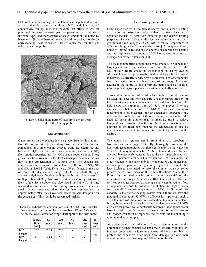
(< 1 week) and depending on orientation has the potential to build a hard, durable scale or a thick, fluffy and low thermal conductivity fouling layer. It is possible that efforts to seal off pots and increase exhaust gas temperatures will introduce different types and mechanisms of scale deposition, as noted by Naess et al. [8], and these influences should be tracked closely for corresponding heat exchanger design optimized for the gas velocity near the probe.
Figure 7. SEM photograph of scale from the upstream side of the fouling probe.
Gas composition Gases present in the exhaust include predominantly air drawn in from the potroom (to obtain under-pressure in the cells), fluorine compounds and other vapors evolved from the electrolyte and feedstock, H2O from moisture in air, alumina, and anodes; SO2 from anode impurities, and CO2/CO due to anode reactions. These gases may be corrosive for the heat exchanger materials, mainly due to the condensation of sulfuric acid. The exhaust gas compositions were measured in September 2009 for CO, SO2, NO and NO2 as listed in Table IV at two different flanges at the duct in front of the dry scrubber using a TESTO 350 M/XL flue gas analyzer. Hydrogen fluoride readings performed simultaneously in September 2009 by Nordural’s online monitoring systems in front of the dry scrubber are also listed in Table IV. Pitting occurred on the surface of the fouling probe made of stainless steel, which indicates that the surface temperature of approximately 50°C may have been below the acid dew point for the exhaust gas. This should be researched further. Table IV. Exhaust gas composition; CO, SO2, NO, NO2, and HF
measurements in front of the dry scrubber. NO and NO2 were below the lowest detection range (4/10 ppm) of the instrument
Sampl. time [min]
CO [ppm]
SO2 [ppm]
NO [ppm]
NO2
[mg/ Nm3]
HF[mg/Nm³]
M1/ flange1
29.0 552.9 70.8 ./. ./.
239 M2/ flange4
30.3 543.3 70.6 ./. ./.
Heat recovery potential Long experience with geothermal energy and a strong existing distribution infrastructure make Iceland a prime location to consider the use of heat from exhaust gas for district heating purposes. Typical Icelandic district heating schemes utilize a geothermal fluid supply at 80°C with a return temperature of 40°C, resulting in a 40°C temperature drop [13]. A typical family home of 150 m2 in Iceland has an energy consumption for heating and hot tap water of around 30,000 kWhth/year, utilizing on average 700 m³ hot water/year [14]. The local communities around the Hydro smelters in Sunndal and Høyanger are utilizing heat recovered from the smelters. In the case of the Nordural smelter in Grundartangi, the nearby town of Akranes, home to approximately six thousand people and several industries, is currently serviced by a geothermal hot water pipeline from the Deildartunguhver hot spring, 62 km away. A gradual decline in the output of this spring and maintenance difficulties make supplanting or replacing the system potentially attractive. Temperature limitations of the filter bags in the dry scrubber must be taken into account when devising a heat exchange strategy for the exhaust gas. Gas inlet temperature to the dry scrubber must be held below the maximum limit of 135°C to prevent filter-bag damage, and below a limit of 110-115°C to meet emissions requirements [15]. Placement of heat exchangers upstream of the dry scrubber could help meet these requirements and reduce the need for false air dilution that is otherwise used to reduce temperatures. However, kinetics of the fluorine reaction with alumina on the filter bags requires the temperature to also be maintained above a lower temperature limit depending on the design. The annual duct temperatures in front of all dry scrubbers at Nordural are in average 75°C. By thoroughly insulating the ductwork gas temperatures will rise significantly, so that values of 90°C-110°C may be obtainable. Ambient temperatures in Iceland are cool but relatively constant due to the maritime climate; with mean temperatures around 0°C in winter and 10°C in summer. At other smelters with higher ambient temperatures and tighter pots, exhaust gas temperatures are generally higher. It is possible that heat exchange may need to take place in a two-stage series process across both sides of the filters (locations A and B in Figure 2), presumably with lower fouling potential on the downstream set. Regardless, with a 10 K temperature difference for heat exchange between exhaust gas and water in counter-flow arrangement, it would be possible to heat about 325 kg/s of water from the 40°C return temperature to 80°C. Addition of this capacity to the district heating system would therefore have the potential to add about 55 MWth, sufficient for supplying roughly 15,000 homes with base load for heat and hot tap water in Iceland. It may be estimated that each smelter pot that consumes 0.9 MW of electrical power could contribute towards a heating/hot water base load of about 29 homes. Exchanger antifouling provisions and proper insulation of pipelines are essential to maintaining a maximum thermal output. As a side benefit the reduction of the gas temperature has the potential to reduce exhaust gas fan power, especially at smelters that rely on sucking in false air upstream of the dry scrubber to protect the expensive filter bags from damage, prolong their operation time, and meet required HF emission levels.
D Technical paper : Heat recovery from the exhaust gas of aluminum reduction cells. TMS 2010

Due to the relatively low temperatures, district heating appears to be the best fit for this kind of heat source. During the course of the study Nordural undertook a comprehensive program to better seal up the pots in order to improve the hooding efficiency. Simultaneously the amperages of both potlines were increased. These changes led to a significant rise in the exhaust gas temperature. Additional efforts in this direction, or new pot designs, will improve the exhaust gas temperature, reduce the exhaust gas flow rate, and increase CO2 concentrations making CO2 capture more economically attractive. In the event that cell exhaust gas temperatures can be raised to 130-150°C or higher, waste heat power generation techniques using technology such as binary cycles may become feasible. The first law energy conversion efficiency at these low temperatures is quite low, i.e. around 10% [16], and in Iceland the availability of low cost power from large-scale hydro and geothermal sources may make this option uncompetitive. However, at other locations where electricity is at a higher premium, or if alternative gas extraction technologies could provide higher temperatures and hence efficiencies, electricity generation may be more appealing.
Conclusion Based on observations at Nordural, the total exhaust gas flow of 912 Nm3/s at a temperature of 100°C has the potential for recovering 55 MWth, if used in a district heating scheme. The heavy dust content of 0.26-0.38 g dust/kg exhaust gas calls for careful antifouling provisions in the design of heat exchangers for these streams. The dust appears to mainly consist of alpha alumina, followed by chiolite, cryolite and kogarkoite, and with trace amounts of fluorite and sodium aluminum fluoride. Although EDS and Macro Elemental analysis indicated substantial carbon, this was not evident using XRD, probably due to it being present in an amorphous form. Modal particle size in the isokinetic samples was determined to be 19.5 μm (by volume), whereas the modal particle size of particles deposited downstream on a fouling probe was noticeably smaller, at 9 μm. For tubes aligned in the cross flow direction, the reduction in overall heat transfer coefficient was observed to drop by 3% on the upstream side and by 29% on the downstream side over a 11 day period. The heat transfer coefficient for the probe as a whole declined close to 7% over this period. The consistency of fouling deposits varied significantly, from loose powder to hard tenacious scale. The interactions of gas and dust compositions on corrosion and fouling aspects should be considered carefully for heat exchanger design. Additional investigations related to the sensitivity of fouling to the effects of gas stream velocity, temperature, and heat exchanger orientation and design are recommended, as well as corrosion evaluations and scale removal techniques. One should aim for a design where fouling is avoided, or at least kept to a minimum, to prevent reductions in heat exchanger efficiency, increases in pressure drop across the heat exchanger, and expensive maintenance.
Acknowledgements We would like to recognize Century Aluminum and the staff at the Nordural smelter for providing support, access and data. This work has been sponsored by Norsk Hydro, which has also been involved in the research work. Specialists at the Icelandic Innovation Center (NMI) also provided valuable assistance.
References 1. Grjotheim, K., Kvande, H., Introduction to aluminium
electrolysis. Düsseldorf : Aluminium Verlag, 2nd edition, 1993.
2. Abbas, H., Taylor, M., Farid, M., and Chen, J. “The impact of cell ventilation on the top heat losses and fugitive emissions in an aluminium smelting cell”. TMS, Light Metals (2009), pp. 551-556.
3. Lorentsen, O-A., Dyroy, A., Karlsen, M., “Handling CO2eq from an aluminium electrolysis cell”. TMS, Light Metals (2009), pp. 263-268.
4. Stern, A. C.: Air Pollution, Analysis, Monitoring and Surveying. New York, London: Academic Press, Volume II, 1968.
5. Dennis, R., Samples, W., “Isokinetic Sampling Probes”. Industrial & Engineering Chemistry 49 (1957), pp 294-302.
6. Gimbun, J., Choong, T., Fakhru’l-razi A., Chuah T., “Prediction of the effect of dimension, particle density, temperature, and inlet velocity on cyclone collection efficiency”. Jurnal Teknologi 40 (F) (2004), pp. 37-50.
7. Reference standards for X-Ray Microanalysis: No. 2440 and 3587. Micro-Analysis Consultants Limited, Unit 3, Edison Road, St Ives Industrial Estate, St Ives, Cambridgeshire PE17 4LF, UK.
8. Naess, E., Slungaard, T., Moxnes B., Sonju O., “Experimental investigation of particulate fouling in waste heat recovery from the aluminum industry”. International Heat Transfer Conference (2006).
9. Hakonarsson, H., “Fouling Probe”. Final project in Taeknifraedi: Reykjavik University, Reykjavik, Iceland, 2009.
10. Temu, A. K., Naess, E., Sonju, O.K., “Development and testing of a probe to monitor gas-side fouling in cross flow”. Heat Transfer Engineering 23 (2002), pp. 50-59.
11. Gudmundsson, H., “Improving anode cover material quality at Nordural - Quality tools and measures”. TMS, Light Metals (2009), pp. 467-472.
12. Temu, A. K., Experimental and theoretical study of particle deposition onto a cylinder in cross flow. (Phd thesis in Department of Thermal Energy and Hydropower : Faculty of Mechanical Engineering: Norwegian University of Science and Technology, Norway, 1998).
13. Karlsson, T., Ragnarsson, A., “Use of Very Low Temperature Geothermal Water in Radiator Heating Systems”. Proc. World Geothermal Congress (1995), pp. 2193-2198.
14. Ragnarsson, A., “Geothermal power development”. Postgraduate lecture, University of Iceland, Reykjavik, Iceland, 2008.
15. Sorhuus, W., Wedde G., “Pot gas heat recovery and emission control”. TMS, Light Metals (2009), pp. 281-286.
16. Dipippo, R., “Ideal thermal efficiency for geothermal binary power plants.” Geothermics 36 (2007), pp. 276-285.
D Technical paper : Heat recovery from the exhaust gas of aluminum reduction cells. TMS 2010