Embed Size (px)
Citation preview

HEART SOUND SEGMENTATION USINGSIGNAL PROCESSING METHODS
a thesis submitted to
the graduate school of engineering and science
of bilkent university
in partial fulfillment of the requirements for
the degree of
master of science
in
computer engineering
By
Devrim Sahin
July, 2015
HEART SOUND SEGMENTATION USING SIGNAL PROCESSING
METHODS
By Devrim Sahin
July, 2015
We certify that we have read this thesis and that in our opinion it is fully adequate,
in scope and in quality, as a thesis for the degree of Master of Science.
Assoc. Prof. Dr. Hakan Ferhatosmanoglu (Advisor)
Assoc. Prof. Dr. Cigdem Gunduz Demir
Assist. Prof. Dr. Aybar C. Acar
Approved for the Graduate School of Engineering and Science:
Prof. Dr. Levent OnuralDirector of the Graduate School
ii

ABSTRACT
HEART SOUND SEGMENTATION USING SIGNALPROCESSING METHODS
Devrim Sahin
M.S. in Computer Engineering
Advisor: Assoc. Prof. Dr. Hakan Ferhatosmanoglu
July, 2015
Heart murmurs are pathological heart sounds that originate from blood flow-ing with abnormal turbulence due to physiological defects of the heart, and arethe prime indicator of many heart-related diseases. Murmurs can be diagnosedvia auscultation; that is, by listening with a stethoscope. However, manual detec-tion and classification of murmur requires clinical expertise and is highly proneto misclassification. Although automated classification algorithms exist for thispurpose; they heavily depend on feature extraction from ‘segmented’ heart soundwaveforms. Segmentation in this context refers to detecting and splitting cardiaccycles. However, heart sound signal is not a stationary signal; and typically hasa low signal-to-noise ratio, which makes it very difficult to segment using no ex-ternal information but the signal itself. Most of the commercial systems requirean external electrocardiography (ECG) signal to determine S1 and S2 peaks, butECG is not as widely available as stethoscopes. Although algorithms that pro-vide segmentation using sound alone exist, a proper comparison between thesealgorithms on a common dataset is missing. We propose several modifications tomany of these algorithms, as well as an evaluation method that allows a unifiedcomparison of all these approaches. We have tested each combination of algo-rithms on a real data set [1], which also provides manual annotations as groundtruth. We also propose an ensemble of several methods, and a heuristic for whichalgorithm’s output to use. Whereas tested algorithms report up to 62% accuracy,our ensemble method reports a 75% success rate. Finally, we created a tool namedUpBeat to enable manual segmentation of heart sounds, and construction of aground truth dataset. UpBeat is a starting medium for auscultation segmenta-tion, time-domain based feature extraction and evaluation; which has automaticsegmentation capabilities, as well as a minimalistic drag-and-drop interface whichallows manual annotation of S1 and S2 peaks.
Keywords: Heart sound, Segmentation, Fourier, Wavelet transform.
iii
OZET
ISARET ISLEME YONTEMLERI KULLANILARAK
KALP SESI BOLUTLEME
Devrim Sahin
Bilgisayar Muhendisligi, Yuksek Lisans
Tez Danısmanı: Assoc. Prof. Dr. Hakan Ferhatosmanoglu
Temmuz, 2015
Kalpte olusan fiziksel bozuklukların kan akısını etkilemesi sonucu olusanseslere ufurum denir. Ufurumler bircok kalp hastalıgının birincil habercisidir.Kalp seslerini stetoskop aracılıgıyla dinlemek (oskultasyon) suretiyle ufurumleruzerinden teshis yapılabilse de, bu tur teshisler tıbbi uzmanlık gerektirmek-tedir ve hatalara oldukca acıktır. Literaturde otomatik sınıflandırma algorit-maları onerilmis olsa da; ses dalgabicimlerinden ayıklanacak olan ozniteliklerinkalp atımı icerisindeki konumları teshis acısından onem tasıdıgı icin, oncelikle bir-inci ve ikinci kalp seslerinin konumlarını belirlemek ve buna gore oznitelik secmekgereklidir. Kalp atımlarının saptanması ve ayrıstırılması islemine bolutleme(segmentasyon) adı verilmektedir. Kalp sinyalinin organik yapısı dolayısıylaongorulebilir bir frekans-zaman profilinin olmaması, sadece ses kaydını kullanarakbolutleme isini zorlastırmaktadır. Bircok ticari sistemde harici olarak bir elek-trokardiyografi (EKG) sinyali de kaydedilse de, EKG aygıtlarının stetoskop kadaryaygın olmaması bu sistemlerin erisilebilirligini dusurmektedir. Yalnızca kalpsesi kullanarak bolutleme yapan algoritmalar olsa da, bu algoritmaların hepsininuzerinde sonuc sundugu ortak bir veritabanı yoktur. Bu calısmada, var olan al-goritmalara cesitli uyarlamaların yanı sıra, bu cesitlemeleri karsılastırmak icinkullanılabilecek bir degerlendirme olcutu oneriyoruz. Ornekleri icin elle yapılmısbolutlemelerin mevcut oldugu Pascal [1] veritabanından alınmıs 66 kayıt uzerindebu yaklasımların tum kombinasyonlarını karsılastırıyoruz. Bunun yanı sırabirkac yontemi karıstırarak sonuc kalitesini artırmayı amaclayan bir birlesimde oneriyoruz. Karsılastırdıgımız tekil algoritmalar %62’ye varan basarılargosterirken onerdigimiz birlesim ile %75’lik bir basarı oranına ulastık. Sonolarak, Pascal gibi denetleme amaclı veritabanlarının kolayca ve hatasız sekildeolusturulabilmesi icin bir arac urettik.
Anahtar sozcukler : Kalp sesi, Bolutleme, Fourier, Dalgacık donusumu.
iv
Acknowledgement
“Think where man’s glory most begins and ends, and say my glory was I had such
friends.”
—William Butler Yeats
Of all the people I have met in my life, the two very best are the two very
first. Mom, dad; you are absolutely irreplaceable to me. Thank you for being
exceptionally amazing parents, I am proud to be your child.
My supervisor and role model, Prof. Dr. Hakan Ferhatosmanoglu; thank you
for your endless patience, wisdom, support; and the sense of direction you have
provided me whenever I felt devoid of purpose.
I thank every teacher and mentor of mine with endless gratitude for their
selflessness. Especially Fikret Ekin, Banu Ozdemir, Metin Tiraki, Sedat Kayak,
Hurriyet Yıldız and Inci Yıldız; I owe you my endless passion for knowledge. You
will always be the moons on a bright sky by which I find my path.
All my precious friends (whom I cannot thank one by one, for I have many);
thank you for being there for me. If I have ever made any you happy in return,
then mine is a life well spent. Musa Tunc Arslan; your absence would hurt.
Coffee mugs and teapots of the world; whatever I did, you have always been
by my side. I love you unconditionally.
So long, and thanks for all the fish.
(This study is financially supported by TUBITAK National Scholarship Programme
for MSc Students.)
v

Contents
1 Introduction 1
2 Mathematical Background 7
2.1 Time-Frequency Transforms . . . . . . . . . . . . . . . . . . . . . 7
2.1.1 Fourier Transform . . . . . . . . . . . . . . . . . . . . . . . 7
2.1.2 Short-Time Fourier Transform and Spectrogram . . . . . . 9
2.1.3 Wavelet Transform . . . . . . . . . . . . . . . . . . . . . . 10
2.1.4 S-Transform . . . . . . . . . . . . . . . . . . . . . . . . . . 16
2.1.5 Constant-Q Transform . . . . . . . . . . . . . . . . . . . . 16
2.2 Maximal Marginal Relevance . . . . . . . . . . . . . . . . . . . . . 17
3 Related Work 19
3.1 ECG Segmentation . . . . . . . . . . . . . . . . . . . . . . . . . . 21
3.2 PCG Segmentation . . . . . . . . . . . . . . . . . . . . . . . . . . 22
3.2.1 Step 0: Preprocessing . . . . . . . . . . . . . . . . . . . . . 24
vi

CONTENTS vii
3.2.2 Step 1: Time-Frequency Transformation . . . . . . . . . . 25
3.2.3 Step 2: Transformation to a Non-Negative Domain . . . . 26
3.2.4 Step 3: Envelope Detection . . . . . . . . . . . . . . . . . 26
3.2.5 Step 4: Picking Up Peaks . . . . . . . . . . . . . . . . . . 28
3.2.6 Step 5: Rejection and Merging of Extra Peaks . . . . . . . 28
3.2.7 Results . . . . . . . . . . . . . . . . . . . . . . . . . . . . . 30
4 Data Acquisition and Annotation 32
4.1 UpBeat: Heart Sound Segmentation and Annotation Tool . . . . 33
5 Implementation of the Heart Sound Segmentation Algorithms 41
5.1 Algorithms . . . . . . . . . . . . . . . . . . . . . . . . . . . . . . . 41
5.1.1 The Generic 6-Step Algorithm . . . . . . . . . . . . . . . . 42
5.1.2 MMR . . . . . . . . . . . . . . . . . . . . . . . . . . . . . 43
6 Evaluation and Conclusion 47
6.1 Dataset . . . . . . . . . . . . . . . . . . . . . . . . . . . . . . . . 47
6.2 Evaluation . . . . . . . . . . . . . . . . . . . . . . . . . . . . . . . 48
6.2.1 Method 1 . . . . . . . . . . . . . . . . . . . . . . . . . . . 49
6.2.2 Method 2 . . . . . . . . . . . . . . . . . . . . . . . . . . . 49
6.2.3 Method 3 . . . . . . . . . . . . . . . . . . . . . . . . . . . 52
CONTENTS viii
6.3 Results . . . . . . . . . . . . . . . . . . . . . . . . . . . . . . . . . 52
6.3.1 Metric 1 . . . . . . . . . . . . . . . . . . . . . . . . . . . . 53
6.3.2 Metric 2 . . . . . . . . . . . . . . . . . . . . . . . . . . . . 54
6.3.3 Metric 3 . . . . . . . . . . . . . . . . . . . . . . . . . . . . 55
6.4 Ensemble . . . . . . . . . . . . . . . . . . . . . . . . . . . . . . . 56
6.5 Conclusion . . . . . . . . . . . . . . . . . . . . . . . . . . . . . . . 57
List of Figures
1.1 The anatomy of mammal heart . . . . . . . . . . . . . . . . . . . 1
2.1 Fourier transform . . . . . . . . . . . . . . . . . . . . . . . . . . . 9
2.2 Wavelet transform - STFT Comparison . . . . . . . . . . . . . . . 11
2.3 Wavelet transform . . . . . . . . . . . . . . . . . . . . . . . . . . 12
2.4 An example to the Haar wavelet transform . . . . . . . . . . . . . 13
2.5 Frequency responses of Haar transform . . . . . . . . . . . . . . . 14
2.6 An example to the Daubechies-4 wavelet transform . . . . . . . . 15
2.7 Maximal marginal relevance example . . . . . . . . . . . . . . . . 18
3.1 Normal heart sound waveform . . . . . . . . . . . . . . . . . . . . 19
3.2 Non-negative transforms . . . . . . . . . . . . . . . . . . . . . . . 26
4.1 Initial screen of UpBeat . . . . . . . . . . . . . . . . . . . . . . . 34
4.2 Main screen of UpBeat . . . . . . . . . . . . . . . . . . . . . . . . 35
4.3 UpBeat menu . . . . . . . . . . . . . . . . . . . . . . . . . . . . . 35
ix
LIST OF FIGURES x
4.4 UpBeat themes . . . . . . . . . . . . . . . . . . . . . . . . . . . . 36
4.5 Zooming on a signal . . . . . . . . . . . . . . . . . . . . . . . . . 37
4.6 Resetting segmentation . . . . . . . . . . . . . . . . . . . . . . . . 38
4.7 Audio playback . . . . . . . . . . . . . . . . . . . . . . . . . . . . 38
4.8 Exporting to an .sgm file . . . . . . . . . . . . . . . . . . . . . . . 39
4.9 Feature display tool . . . . . . . . . . . . . . . . . . . . . . . . . . 40
5.1 The generic 6-step algorithm . . . . . . . . . . . . . . . . . . . . . 44
6.1 Evaluation Method 1 . . . . . . . . . . . . . . . . . . . . . . . . . 50
6.2 Evaluation Method 2 . . . . . . . . . . . . . . . . . . . . . . . . . 51

List of Tables
3.1 Decimation schemes of various PCG segmentation algorithms . . . 24
6.1 Evaluation scores of the top-20 algorithms, according to Evaluation Metric 1 53
6.2 Evaluation scores of the top-20 algorithms, according to Evaluation Metric 2 54
6.3 Evaluation scores of the top-20 algorithms, according to Evaluation Metric 3 55
6.4 Methods selected for the ensemble . . . . . . . . . . . . . . . . . . 57
xi

Chapter 1
Introduction
Figure 1.1: The anatomy of mammal heart
In living organisms, distribution and transportation of blood is conducted by the
cardiovascular system. The circulation of blood allows the cardiovascular system
to transport oxygen to and carbon dioxide from cells; distribute nutrients, hor-
mones, blood cells; as well as fight pathogens, regulate acidity, body temperature,
glucose concentration etc. [2]
Cardiovascular system consists of the heart, blood and blood vessels [3]. Heart
is the central component of the circulatory system. It pumps oxygenated blood
into the cells and collects oxygen-poor blood to the lungs. Correct operation of
the heart is, thus, vitally important. Among the 57 million deaths that occurred
globally in 2008, 36 million were due to non-communicable diseases (NCDs),
1

of which the most common is cardiovascular diseases [4]. Turkey’s profile in
fighting heart diseases is not promising either; where NCDs are accounted for
approximately 86% of total deaths, the highest of which is cardiovascular diseases
with a proportion of 47% [5]. This makes detection and classification of heart
diseases very important.
Figure 1.1 depicts the mammal heart. The left and right sides of the heart
are isolated from each other; and perform slightly different tasks simultaneously.
Each side is divided into two chambers with a valve in between. The smaller
chambers that are on top are named the atria, whereas the lower chambers are
called ventricula [6]. The blood enters the heart through the atria on both sides;
the right side receives oxygen-poor blood collected from the body, whereas the
left-side receives oxygen-rich blood collected from the lungs. When both atriums
contract, the blood is pumped into the ventricles on both sides. After this, the
ventricular muscles contract strongly and pump the blood into the pulmonary
trunk on the right, which carries oxygen-poor blood into the lungs; and aorta
on the left, which distributes oxygen-rich blood to the body. During these two
contractions, two audible sounds are generated, called ‘lub’ and ‘dub’ respectively.
There exist four valves in between these chambers which prevent blood from
leaking backwards during each of the contractions. [2]
Heart is a complicated machinery that may fail to operate correctly on many lev-
els. Putting severe cases as traumatic ruptures and heart attacks aside, anatomi-
cal or developmental defects can occur. One example is the failure of heart valves
to properly close, in which case some of the blood flows backwards turbulently.
Another problem may occur in the thin blood vessel named Ductus Arteriosus
between the pulmonary artery and aorta (depicted in Figure 1.1). This vessel is
used in fetuses to bypass the lungs that are not yet functional, but closes in birth
and becomes the arterial ligament. However, a failure in the developmental stage
can cause this vessel to remain open, leading to the congenital disorder known as
Patent Ductus Arteriosus (PDA), causing shortness of breath and poor growth
etc. [7] Both of these problems present themselves with a characteristic abnormal
sound, known as a heart murmur.
2

There are various tools and techniques available for cardiologists to achieve a
diagnosis, including auscultation, electrocardiography, echocardiography, Holter
monitors, computer tomography, magnetic resonance imaging and so on. How-
ever, most of these options require an expensive setup. For example, magnetic
resonance imaging (MRI) requires a medical MRI scanner, which has a cost of
more than $1000 per scan (United States national median cost, excluding in-
surance) [8]. In Turkey, the price the patient is to pay is as low as 72 TRY
[9], but the rest of the expense is then covered by the state. In any case, this
prevents medical doctors from asking for an MRI scan immediately for every pa-
tient. Therefore, even when cardiologists suspect that a more complicated test is
required, they decide to resort to simpler, less expensive methods as a first step.
The simplest, cheapest, and therefore most commonly used technique is known
as cardiac auscultation.
Cardiac auscultation (or “auscultation”, shortly) is the process of listening to
heart sounds using a simple equipment such as a stethoscope. If these heart
sounds are recorded, the recording is called a phonocardiogram, or PCG. As a
medical test, auscultation is fairly simple to apply; and the only required equip-
ment being the stethoscope, it is virtually cost-free. This means that even in
third-world countries, auscultation has a very broad availability.
The problem with auscultation, however, is that the interpretation of the sounds
heard (or recorded) is not trivial. Diagnosis through cardiac auscultation requires
years of clinical expertise and proper education to conduct properly. Furthermore,
even with years of experience, the analysis remains critically subjective. It is re-
ported that up to 80% of diagnoses made by expert physicians using auscultation
are actually incorrect [10]. The main reason the error rates are as high as reported
is that auscultatory analysis is very inconclusive. Since the well-being of the pa-
tients is involved, physicians tend to make Type-I errors (false alarms) almost
deliberately, in order to avoid missing any potential abnormalities. This is a nec-
essary attitude when the cost of Type-II errors (misses) is high (e.g. advancement
of diseases, possibly death).
3
Given that auscultation is a comparably inconclusive test, one can argue that in-
creasing the reliability of the test by developing an objective auscultation analysis
approach would allow the physicians to avoid a significant amount of expense,
creating a relief on the healthcare budgets of especially less developed countries
[10]. Such a system would then increase the confidence of the diagnosis, and thus
broaden availability of cardiac diagnostics even where more complicated tests are
not easily accessible. With the electronic stethoscopes becoming more available
by the day, it is now possible to discuss the possibility of an computer-aided af-
fordable analysis tool that will provide objective measures of heart disease risks.
There have been numerous approaches for detecting heart diseases using a range
of signal processing and machine learning techniques. The majority of these
algorithms share a three-step approach; involving (1) cardiac cycle segmentation,
(2) feature extraction, and (3) classification. The last two steps are well-studied
in the literature; many different machine learning approaches including but not
limited to support vector machines, artificial neural networks, even decision trees
were applied on the problem of the classification of heart sounds once they are
segmented [6, 10–26], however the approaches to the segmentation step remain
outdated. Bentley et al. acknowledge that once the segmentation challenge is
solved, the following steps will be “considerably easier”[1].
Cardiac cycle segmentation (the details of which will be discussed in length) is
detection of the ‘beats’ of heart, such that any abnormalities determined can be
taken into consideration regarding its location. Location of an abnormal com-
ponent in the phonocardiogram is a very important feature for classification of
heart murmurs. Murmurs are one of the most common abnormalities that can be
detected via auscultation. These are audible turbulent sounds which may be gen-
erated by leaking heart valves, holes in cardiac muscles, developmental disorders,
and a myriad of other conditions [7]. For all of these cases, the characteristics of
the murmur change drastically. Murmurs can appear at different locations in the
cardiac cycle, may increase or decrease in amplitude, be constantly loud; or may
be observed at different frequency bands and different auscultation locations. All
of these features help detecting the nature of the murmur.
4

However, trying to find the characteristics of murmur using only one cardiac cycle
is not a reliable approach. Heart sound recordings are rarely (if ever) devoid of
noise; moreover, the statistical properties of the noise present in such signals re-
main to be unpredictable: Additive white noise, lung sounds, mechanical sounds,
loud peaks originating from physical movement of the stethoscope, even reverber-
ations of the original heart sound echoing from internal tissues frequently appear
in the phonocardiogram. Hence, it is critical to have a robust segmentation algo-
rithm that is capable of correctly detecting as many cardiac cycles as possible in
order to make reliable diagnoses.
In this study, we investigate several approaches to heart sound segmenta-
tion using only phonocardiogram recordings. The initial approach is a six-
step algorithm, of which majority of the work in the literature is a variation
[6, 11, 13, 15–19, 23, 25, 27–32]. These six steps include preprocessing (resampling
and normalization), a time-frequency transform (selection of relevant frequency
bands), rectification (transformation of the signal to a non-negative domain that
represents magnitude), envelope detection (elimination of high frequency modu-
lation), peak selection (thresholding and detection of peak candidates), and peak
merging (elimination of redundant peaks and classification of the remaining can-
didates as S1/S2). Throughout the literature, different studies have proposed
different methods for each of these six steps. We provide a comparison of these
works by implementing all of these variations and testing every combination on a
common real data set [1]. As a contribution, we also propose a modified version
of the Maximal Marginal Relevance (MMR) method [33], which is widely used in
the information retrieval context, as an alternative to the traditional approach.
We define the similarity metrics that MMR uses such that diverse peaks are
picked, maximizing both their amplitudes and temporal distances to each other.
We also introduce an ensemble of the aforementioned methods in order to boost
the algorithm’s performance. For our tests, we use the annotated Pascal heart
sound data set [1] and score each algorithm using a common evaluation metric
that we propose. Finally, we developed an application that helps constructing
and annotating a ground truth data set for heart sound segmentation, which is
also a powerful tool for waveform visualization and playback, useful in providing
5
an intuition for cardiac auscultation.
The rest of this thesis is organized as follows:
Chapter 2 provides a mathematical background for the signal processing tech-
niques required for the discussion of our work.
Chapter 3 formally presents the problem, challenges and limitations; and sum-
marizes the methodology and results of the related work in cardiac cycle
segmentation.
Chapter 4 introduces UpBeat, a heart sound signal visualization, playback and
annotation tool that we have developed.
Chapter 5 discusses the implementation of the heart sound segmentation algo-
rithms in detail.
Chapter 6 explains the dataset, introduces our evaluation metric; then lists and
discusses the results for both individual methods and the ensemble. Finally
we conclude by discussing future work.
6

Chapter 2
Mathematical Background
In this section we will describe most of the approaches taken in the related work
and this study. Although topics such as Fourier Transform are mentioned for the
sake of completeness, a certain level of knowledge of signal processing is assumed
with the intent of keeping the discussion brief and to-the-point.
2.1 Time-Frequency Transforms
Since a heart sound recording consists of both relevant and irrelevant information
of different frequencies, it is a common practice to perform a time-frequency
transform on the initial heart sound signal in order to filter and de-noise the
original signal. Several time-frequency transform methods are discussed below,
after a brief discussion of the Fourier transform.
2.1.1 Fourier Transform
Fourier transform is an operation that matches a signal onto the orthogonal
Fourier space [34]. What it accomplishes is representing a time-domain signal
7
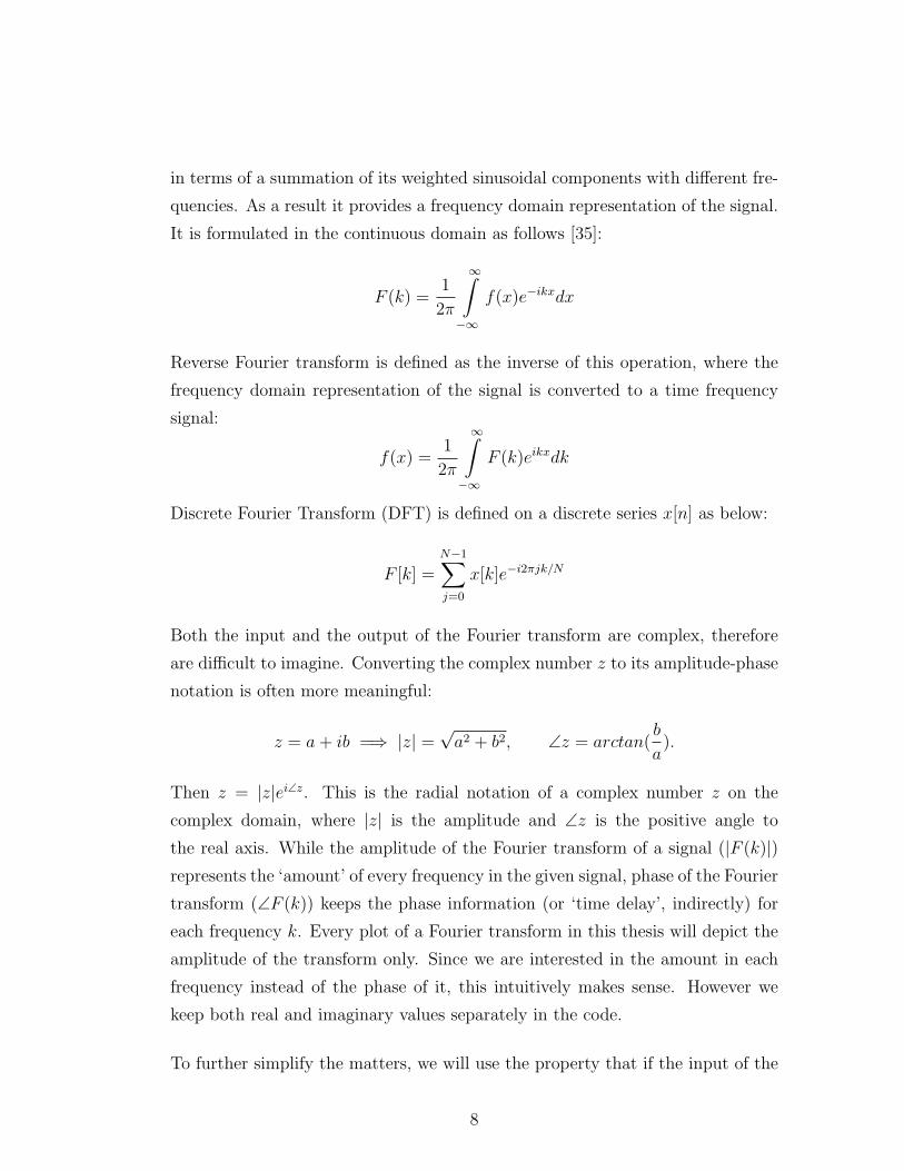
in terms of a summation of its weighted sinusoidal components with different fre-
quencies. As a result it provides a frequency domain representation of the signal.
It is formulated in the continuous domain as follows [35]:
F (k) =1
2π
∞∫
−∞
f(x)e−ikxdx
Reverse Fourier transform is defined as the inverse of this operation, where the
frequency domain representation of the signal is converted to a time frequency
signal:
f(x) =1
2π
∞∫
−∞
F (k)eikxdk
Discrete Fourier Transform (DFT) is defined on a discrete series x[n] as below:
F [k] =N−1∑
j=0
x[k]e−i2πjk/N
Both the input and the output of the Fourier transform are complex, therefore
are difficult to imagine. Converting the complex number z to its amplitude-phase
notation is often more meaningful:
z = a+ ib =⇒ |z| =√a2 + b2, ∠z = arctan(
b
a).
Then z = |z|ei∠z. This is the radial notation of a complex number z on the
complex domain, where |z| is the amplitude and ∠z is the positive angle to
the real axis. While the amplitude of the Fourier transform of a signal (|F (k)|)represents the ‘amount’ of every frequency in the given signal, phase of the Fourier
transform (∠F (k)) keeps the phase information (or ‘time delay’, indirectly) for
each frequency k. Every plot of a Fourier transform in this thesis will depict the
amplitude of the transform only. Since we are interested in the amount in each
frequency instead of the phase of it, this intuitively makes sense. However we
keep both real and imaginary values separately in the code.
To further simplify the matters, we will use the property that if the input of the
8

Figure 2.1: On the left is f1(t) and its Fourier transform. On the right is f2(t)and its Fourier transform. The amplitudes on the frequency domain are identical.
Fourier transform is strictly real, the output is symmetrical along the y-axis, that
is; F (k) = F (−k) iff ℜ{f(x)} = f(x). For our application, it is a given that the
recorded data is real. Therefore it is possible to consider only positive frequencies
for a real input, since the negative side will be redundant.
2.1.2 Short-Time Fourier Transform and Spectrogram
Fourier transform is informative for signals where the frequency distribution of the
signal does not change significantly. For other signals where there the frequencies
that the signal consists of, or their amplitudes change; the result will become a
superposition of them. Consider two signals as follows: In the first signal, we
have f1(t) = u(−t)cos(2π10t) + u(t)cos(2π20t), where u(t) is the step function.
This signal is a cosine with a 10Hz frequency up to t = 0, then changes its
frequency into 20Hz. Also let f2(t) = u(t)cos(2π10t) + u(−t)cos(2π20t), that is,the frequency drops from 20Hz to 10Hz at t = 0. The Fourier transforms of these
two signals F1(k) and F2(k) are equivalent, in that |F1(k)| = |F2(k)| (see Figure
2.1). Therefore it is said that Fourier transform loses the time information.
For many applications, we want to keep the time information; that is, we have a
signal of which the frequency distribution is dynamic and should be attributed to
time itself. That is to say, we would like to find out which frequencies are present
at which time. One example to this is finding the notes of a song: Finding which
9
notes are present in the song is never enough, we also would like to know their
locations in time to analyse a song. Therefore we need a function that maps a
time-domain signal onto the time-frequency domain.
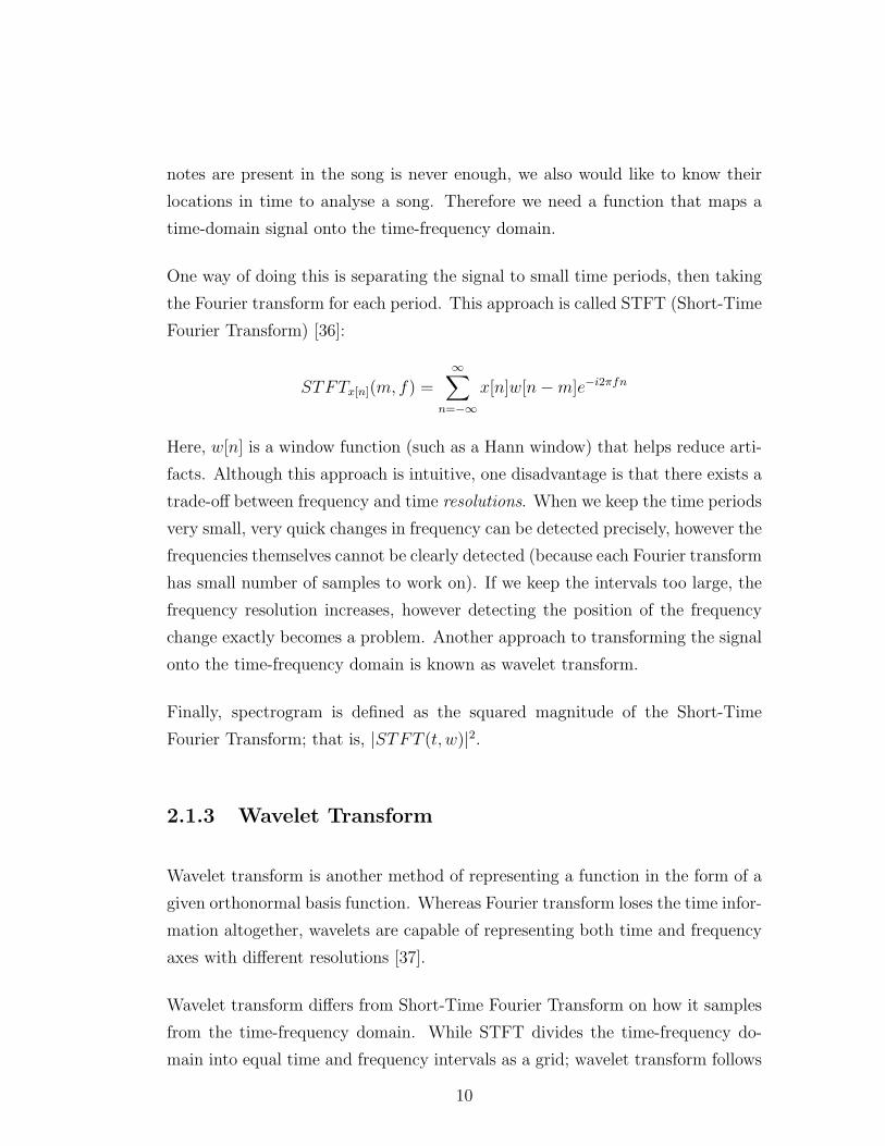
One way of doing this is separating the signal to small time periods, then taking
the Fourier transform for each period. This approach is called STFT (Short-Time
Fourier Transform) [36]:
STFTx[n](m, f) =∞∑
n=−∞
x[n]w[n−m]e−i2πfn
Here, w[n] is a window function (such as a Hann window) that helps reduce arti-
facts. Although this approach is intuitive, one disadvantage is that there exists a
trade-off between frequency and time resolutions. When we keep the time periods
very small, very quick changes in frequency can be detected precisely, however the
frequencies themselves cannot be clearly detected (because each Fourier transform
has small number of samples to work on). If we keep the intervals too large, the
frequency resolution increases, however detecting the position of the frequency
change exactly becomes a problem. Another approach to transforming the signal
onto the time-frequency domain is known as wavelet transform.
Finally, spectrogram is defined as the squared magnitude of the Short-Time
Fourier Transform; that is, |STFT (t, w)|2.
2.1.3 Wavelet Transform
Wavelet transform is another method of representing a function in the form of a
given orthonormal basis function. Whereas Fourier transform loses the time infor-
mation altogether, wavelets are capable of representing both time and frequency
axes with different resolutions [37].
Wavelet transform differs from Short-Time Fourier Transform on how it samples
from the time-frequency domain. While STFT divides the time-frequency do-
main into equal time and frequency intervals as a grid; wavelet transform follows
10

Figure 2.2: Comparison of short-time Fourier transform with wavelet transformin terms of how they partition the time-frequency domain
a dyadic layout where it allocated higher frequencies more samples, whereas fre-
quency ranges are more refined for lower frequencies. An example is given in
Figure 2.2. As it can be seen, wavelet transform actually applies a more rea-
sonable trade-off between time and frequency resolutions, by having more time
samples where frequencies change rapidly (high-frequency components), and vice
versa. Wavelet transform depends on two functions called the mother wavelet
function and the scaling function [37], and different functions can provide differ-
ent wavelets, each of which might be more appropriate for a certain task than
others. At each step, the input signal is passed through a high-pass filter and a
low-pass filter, after which both outputs are downsampled by 2. The process is
iterated on the low-frequency side until the size of the coefficient is equal to 1.
Figure 2.3 depicts the process, and a simple example is described while discussing
Haar wavelets.
2.1.3.1 Haar Wavelet
Haar wavelet the simplest form of wavelet transform.
11

Figure 2.3: Wavelet transform. At each step, detail and approximation coeffi-cients are generated with half the input length. Approximation coefficients areapplied the same process until the output length is 1.
The mother wavelet function for Haar transform is defined as:
ψ(t) =
1 if 0 ≤ t < 12,
−1 if 12≤ t < 1,
0 otherwise.
and the scaling function is:
φ(t) =
1 if 0 ≤ t < 1,
0 otherwise.
An example of the Haar wavelet decomposition on a discrete signal is given in
Figure 2.4. In the first step, each pair of elements effectively generate two coeffi-
cients, such that a1[t] =12I[2t] + 1
2I[2t + 1] and d1[t] =
12I[2t]− 1
2I[2t + 1] (for a
correct Haar transform each of these equations should have been multiplied with√2 for energy preservation but we will omit this detail for simplicity). Effectively,
a low pass filter and a high-pass filter with cut-off frequencies fc = fs/4 are ap-
plied onto the input (the frequency responses of which can be seen in Figure 2.5),
then the result is downsampled with a factor of two. The a1 are the 1st level
12
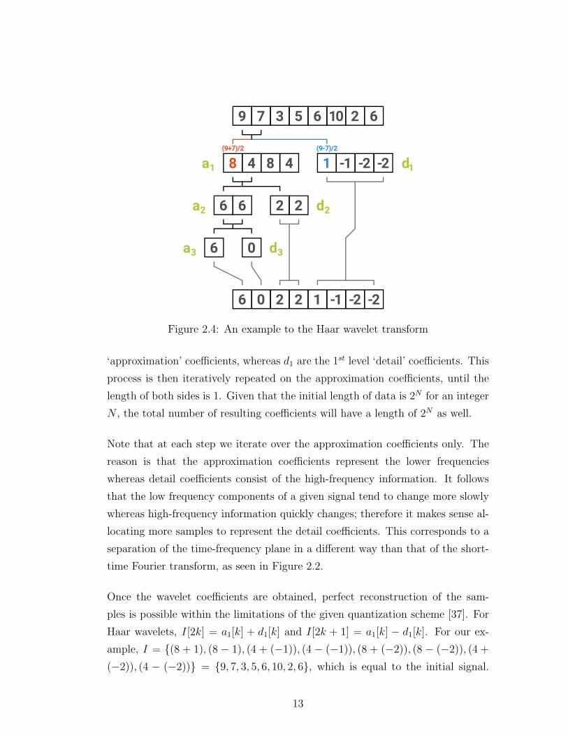
Figure 2.4: An example to the Haar wavelet transform
‘approximation’ coefficients, whereas d1 are the 1st level ‘detail’ coefficients. This
process is then iteratively repeated on the approximation coefficients, until the
length of both sides is 1. Given that the initial length of data is 2N for an integer
N , the total number of resulting coefficients will have a length of 2N as well.
Note that at each step we iterate over the approximation coefficients only. The
reason is that the approximation coefficients represent the lower frequencies
whereas detail coefficients consist of the high-frequency information. It follows
that the low frequency components of a given signal tend to change more slowly
whereas high-frequency information quickly changes; therefore it makes sense al-
locating more samples to represent the detail coefficients. This corresponds to a
separation of the time-frequency plane in a different way than that of the short-
time Fourier transform, as seen in Figure 2.2.
Once the wavelet coefficients are obtained, perfect reconstruction of the sam-
ples is possible within the limitations of the given quantization scheme [37]. For
Haar wavelets, I[2k] = a1[k] + d1[k] and I[2k + 1] = a1[k] − d1[k]. For our ex-
ample, I = {(8 + 1), (8 − 1), (4 + (−1)), (4 − (−1)), (8 + (−2)), (8 − (−2)), (4 +
(−2)), (4 − (−2))} = {9, 7, 3, 5, 6, 10, 2, 6}, which is equal to the initial signal.
13
0 0.1 0.2 0.3 0.4 0.5 0.6 0.7 0.8 0.9 1
10−2
10−1
100
LPF [0.5,0.5] HPF [0.5,−0.5]
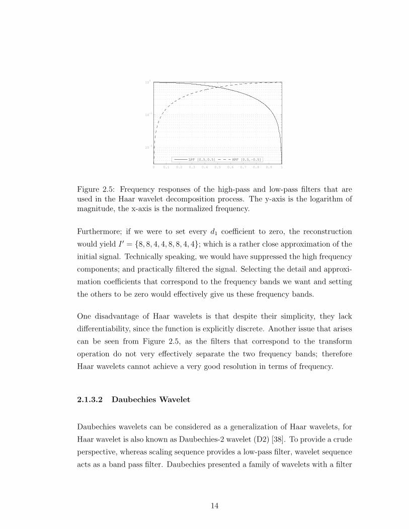
Figure 2.5: Frequency responses of the high-pass and low-pass filters that areused in the Haar wavelet decomposition process. The y-axis is the logarithm ofmagnitude, the x-axis is the normalized frequency.
Furthermore; if we were to set every d1 coefficient to zero, the reconstruction
would yield I ′ = {8, 8, 4, 4, 8, 8, 4, 4}; which is a rather close approximation of the
initial signal. Technically speaking, we would have suppressed the high frequency
components; and practically filtered the signal. Selecting the detail and approxi-
mation coefficients that correspond to the frequency bands we want and setting
the others to be zero would effectively give us these frequency bands.
One disadvantage of Haar wavelets is that despite their simplicity, they lack
differentiability, since the function is explicitly discrete. Another issue that arises
can be seen from Figure 2.5, as the filters that correspond to the transform
operation do not very effectively separate the two frequency bands; therefore
Haar wavelets cannot achieve a very good resolution in terms of frequency.
2.1.3.2 Daubechies Wavelet
Daubechies wavelets can be considered as a generalization of Haar wavelets, for
Haar wavelet is also known as Daubechies-2 wavelet (D2) [38]. To provide a crude
perspective, whereas scaling sequence provides a low-pass filter, wavelet sequence
acts as a band pass filter. Daubechies presented a family of wavelets with a filter
14

Figure 2.6: An example to the Daubechies-4 wavelet transform
size of 2p, by solving the equation below using Bezout theorem [39]:
Hφ(eiw) =
√2
(
1 + e−iw
2
)p
R(eiw)
For p=2, the obtained polynomial is:
P (2− z − z−1
4) = 2− 1
2z − 1
2z−1
of which the roots are 2+√3 and 2−
√3. The discrete-time factorization is then:
hφ[n] =
√2 +
√6
8δ[n] +
3√2 +
√6
8δ[n− 1] +
3√2−
√6
8δ[n− 2] +
√2−
√6
8δ[n− 3]
This gives us the Daubechies-4 wavelet transform, or “D4” in short [39], the
scaling and wavelet functions for which are given in Figure 2.6.
Other wavelet families with different derivations exist, however they are beyond
our scope, because many papers regarding heart sound segmentation use Haar
and D4 wavelets [6, 18, 19, 30]. This makes sense due to a comparison between
wavelet families that revealed that D4 is optimal for heart sound analysis [10].
15
2.1.4 S-Transform
S-Transform is a special variation of STFT such that it allows variable window
sizes [40]. In S-Transform, the window function w(t) is selected as
w(t) =|f |√2πe−t2f2/2
therefore S-transform is defined as
S(t, f) =
∞∫
−∞
x(k)|f |√2πe−(t−k)2f2/2e−i2πfkdk
Although S-transform can provide a good resolution, its computational complex-
ity is as high as O(N3) [41]. An FFT-based implementation has a computational
complexity of O(N2log2(N)) [42], which requires that the acquisition of the en-
tire signal is completed. It is possible to reduce the computational complexity of
S-transform further down to O(Nlog2(N)) using approximations [41]; of which
the implementation might lead to madness [43].
2.1.5 Constant-Q Transform
Constant-Q transform maps the linear frequency domain of a Fast Fourier Trans-
form onto a logarithmic frequency domain [44], such that the kth frequency com-
ponent is at fk = 2k/24fmin. Originally being designed for the geometric posi-
tioning of musical notes, Constant-Q transform separates every octave into 24
intervals; hence the k/24. fmin is the minimum sampled frequency for which in-
formation is desired. The name Constant-Q comes from the fact that the window
on which discrete Fourier transform is performed is selected to have the length
of Q cycles, where Q is a constant. In regular DFT where the kth frequency
component is at kδf , the number of cycles becomes variable, i.e. dependent to k.
16
Here, Q is named the quality factor [45]. The equation becomes the one below:
X[k] =1
N [k]
N [k]−1∑
n=0
W [k, n]x[n]e−i2πQn/N [k]
where
N [k] = Nmax2−k/24
and
W [k, n] = α + (1− α)cos(2πn/N [k]).
which is a Hamming window adapted to the exponential frequency [45].
2.2 Maximal Marginal Relevance
Maximal Marginal Relevance (often abbreviated as MMR) is a method first pro-
posed by Carbonell and Goldstein for text retrieval and summarization [33]. In a
context where sorting a retrieved document set S with respect to their relevance
with a given query Q produces redundant or repetitive results, diversity becomes
a desirable property. A result set is said to be diverse if the retrieved documents
are dissimilar to each other. Diversifying the result set helps represent a large va-
riety of topics in the top results, while avoiding highly similar (or even duplicate)
results.
Assume that for a given document collection C; the information retrieval system
R = IR(C,Q, θ) retrieves a ranked list of documents R that have a similarity
with the query Q above a given relevance threshold θ. then the maximal marginal
relevance is calculated as follows:
MMR = arg maxDi∈R\S
[
λSim1(Di, Q)− (1− λ) maxDj∈S
Sim2(Di, Dj)
]
Here, S is the subset of R that is to be returned. Initially S(0) = ∅. At each
kth iteration, S(k) = S(k−1) ∪MMR. In other words, S contains the elements
that are already picked, and the next element is chosen from the difference set
17
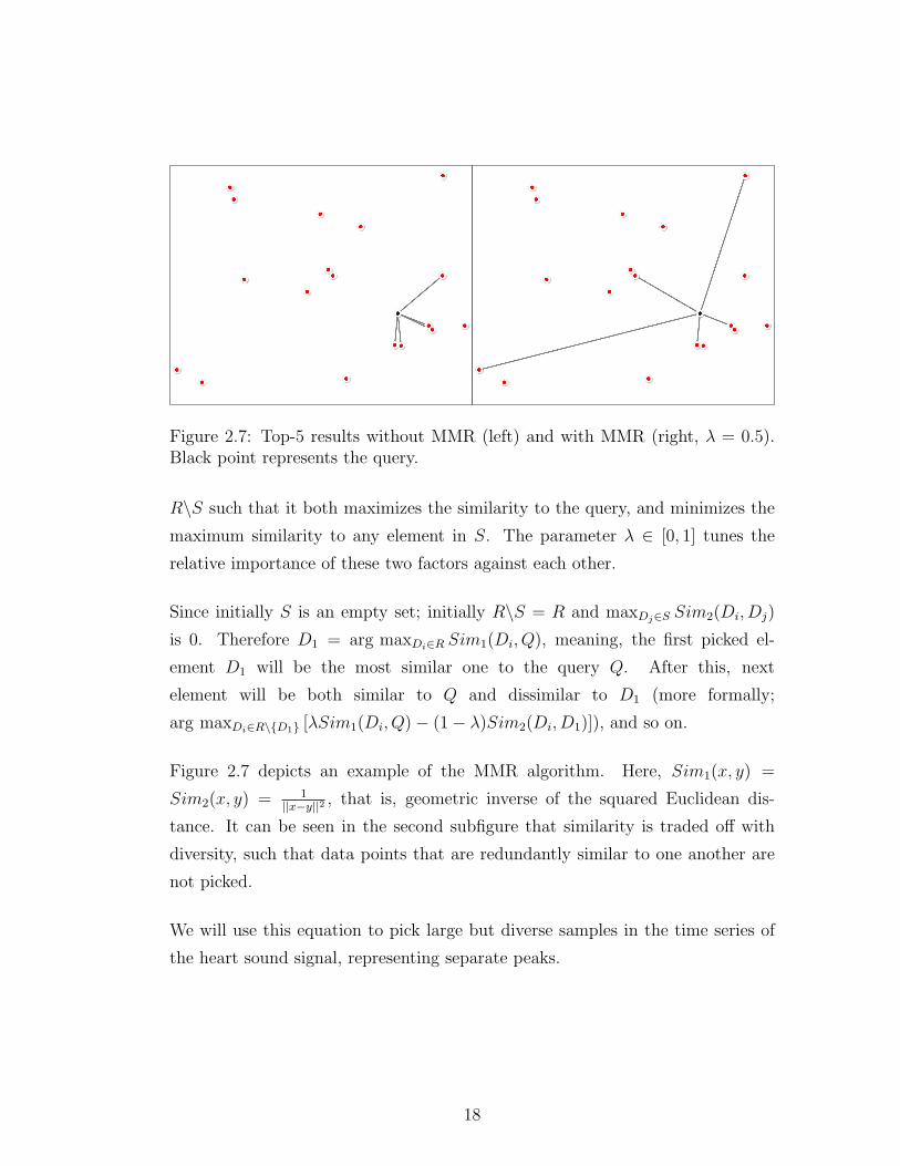
Figure 2.7: Top-5 results without MMR (left) and with MMR (right, λ = 0.5).Black point represents the query.
R\S such that it both maximizes the similarity to the query, and minimizes the
maximum similarity to any element in S. The parameter λ ∈ [0, 1] tunes the
relative importance of these two factors against each other.
Since initially S is an empty set; initially R\S = R and maxDj∈S Sim2(Di, Dj)
is 0. Therefore D1 = arg maxDi∈R Sim1(Di, Q), meaning, the first picked el-
ement D1 will be the most similar one to the query Q. After this, next
element will be both similar to Q and dissimilar to D1 (more formally;
arg maxDi∈R\{D1} [λSim1(Di, Q)− (1− λ)Sim2(Di, D1)]), and so on.
Figure 2.7 depicts an example of the MMR algorithm. Here, Sim1(x, y) =
Sim2(x, y) = 1||x−y||2
, that is, geometric inverse of the squared Euclidean dis-
tance. It can be seen in the second subfigure that similarity is traded off with
diversity, such that data points that are redundantly similar to one another are
not picked.
We will use this equation to pick large but diverse samples in the time series of
the heart sound signal, representing separate peaks.
18
Chapter 3
Related Work
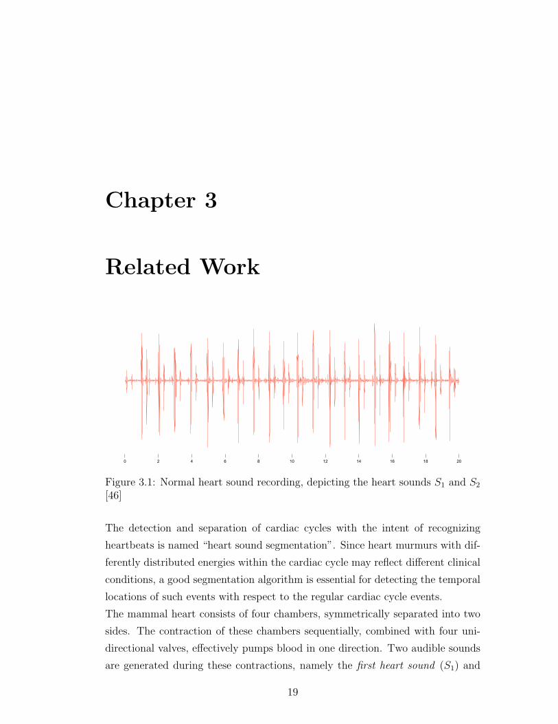
Figure 3.1: Normal heart sound recording, depicting the heart sounds S1 and S2
[46]
The detection and separation of cardiac cycles with the intent of recognizing
heartbeats is named “heart sound segmentation”. Since heart murmurs with dif-
ferently distributed energies within the cardiac cycle may reflect different clinical
conditions, a good segmentation algorithm is essential for detecting the temporal
locations of such events with respect to the regular cardiac cycle events.
The mammal heart consists of four chambers, symmetrically separated into two
sides. The contraction of these chambers sequentially, combined with four uni-
directional valves, effectively pumps blood in one direction. Two audible sounds
are generated during these contractions, namely the first heart sound (S1) and
19

the second heart sound (S2), also occasionally referred to as the ‘lub’ and the
‘dub’ (or ‘dup’) [10]. The interval from one S1 to the next is named a cardiac
cycle. Therefore, each cardiac cycle also contains an S2 peak. This S2 peak sep-
arates the cardiac cycle into two sub-intervals: The interval between S1 and the
following S2 is called a systolic period, whereas the interval between an S2 and
the next S1 is called a diastolic period [6]. In total, a cardiac cycle consists of an
S1 peak, a systolic period, an S2 peak, and a diastolic period in the given order.
Typically, the diastolic period of a given cardiac cycle has a longer duration than
its systolic period.
A heart sound recording may include other sounds, some of which are inaudible
without amplification (for example, S3 and S4). However, S1 and S2 are the only
heart sounds that are commonly expressed in any phonocardiogram, therefore
these two sounds are used by every segmentation algorithm unanimously.
There are various challenges that makes the segmentation task non-trivial. First
of all, heart sound recordings are very noisy, and the assumptions made on a cer-
tain dataset do not hold for another. The source of noise is not only electronic,
but also mechanical; including but not limited to the reverberations of heart
sounds from internal tissues, sharp peaks originating from sudden movements of
the stethoscope, abnormalities in the heart and so on [32]. Attempts at removing
these noises by isolating S1 and S2 sounds in their frequency bands do not work
well, because not only these noises may occur at any frequency band, but also S1
and S2 have different frequencies at every patient and even between cycles [10].
Although attempts have been made to eliminate lung sounds from these record-
ings [32], a reliable method for the removal of the noises in phonocardiograms,
clearly expressing S1 and S2 sounds, remains to be discovered. Therefore, seg-
mentation algorithms try to employ approaches specific to the characteristics of
the heart sound signal, depending heavily on assumptions obtained from medical
observations [6, 15, 17, 23–26, 29–32]. Even though there have been attempts at
designing heart sound classification techniques that do not depend on segmenta-
tion [22], these are reported to show a more robust performance on segmented
data [11]. Therefore, heart sound segmentation remains to be a ‘bottleneck’ for
the performance of many algorithms proposed for heart disease detection and
classification.
20

Another challenge in this line of research is that most of the methods in the
literature have been tested on the datasets that were preprocessed and curated
exclusively and are kept private. This means that there is no guarantee that
a particular method that is tested on a given dataset would provide a similar
performance on another dataset. A proper unification and comparison of these
methods on a common reliable dataset is missing.
There has been extensive work regarding the cardiac cycle segmentation problem
in the last two decades. Two major subsets of these approaches are ECG based
segmentation and PCG segmentation. While ECG segmentation algorithms use
the electrocardiogram signal to segment the phonocardiogram, PCG segmenta-
tion algorithms only receive the heart sound waveform as input.
3.1 ECG Segmentation
There are various heart sound segmentation algorithms using the electrocardio-
gram signal as reference. The advantage of this approach is that ECG signal is
not affected by heart murmurs, which are not electrical events; which makes it
desirable for industrial applications. Dominant peaks in PCG envelope might not
be strongly correlated with cardiac activities in the presence of strong abnormal
sounds [28]. Therefore the performance of a PCG segmentation algorithm can be
rather sensitive to abnormalities when compared to an ECG-aided segmentation
algorithm.
Given the PCG and ECG recordings, an ECG segmentation starts by attempt-
ing at segmenting the ECG signal first [47]. A QRS detection method such as
Tompkins algorithm [12] is applied onto the ECG signal to locate the R waves. It
is observed that R waves are temporally correlated with S1 sounds; therefore S1
sounds in the PCG signal must be in the vicinity of R waves in the ECG signal
[28]. One approach is to call the interval between two R waves a cardiac cycle,
and try to detect S1 and S2 sounds within each cardiac cycle [21]. Another is
called “ECG gating”, and involves searching S1 in the predefined neighborhood
21

of the R waves, then looking for S2 peaks in between [16,17].
There are several advantages of such segmentation algorithms. First of all, the
presence of murmurs does not affect the ECG waveform, thus the performance of
the algorithm [10]. Segmentation of ECG signals is relatively easier and rather
well-studied compared to PCG signals. Finally, reported accuracies of ECG seg-
mentation algorithms are typically higher than PCG segmentation algorithms.
However, these algorithms require an ECG signal to be recorded along with PCG
in the first place. Considering that the design objective we have set was minimiz-
ing hardware requirements to reduce cost and increase availability, this approach
seems misplaced. Also, precise temporal alignment of PCG and ECG signals is
necessary for ECG-aided segmentation algorithms to operate, since they require
that the segmentation obtained in one can be mapped onto the other; which re-
quires a synchronous operation of two independent systems, with good temporal
precision non-trivial to achieve. Finally, even though ECG signal is segmented
properly, S1 and S2 sounds are still looked up on the PCG signal. Especially the
location of S2 can be affected as significantly in the presence of strong murmurs.
Therefore we turn our gaze towards PCG segmentation algorithms permanently
from this point on.
3.2 PCG Segmentation
PCG segmentation algorithms do not use any secondary external signals such as
ECG waveforms to achieve segmentation. Rather, segmentation itself is achieved
directly on the PCG waveform. Since heart abnormalities make themselves ap-
parent on the heart sound, they can affect the performance of the segmentation
algorithm. However, this is the only desirable approach to the problem in terms
of cost, since it does not require the installation, synchronization and acquisi-
tion of any external module such as an electrocardiogram. Since heart sound
signals are highly organic signals, it is very difficult to find a constant factor in
them. Often, the temporal lengths of every systolic and diastolic period deviate.
Even though S1 and S2 are assumed to be highly audible, their amplitudes might
22
change significantly, to the point of disappearance in the presence of certain ab-
normalities. Finally, S1 and S2 peaks do not seem to have fixed frequencies, but
rather present themselves within different frequency bands in two separate car-
diac cycles. These limitations of the heart sound signal led researchers to develop
a rather unique approach to heart sound segmentation. The general approach to
PCG segmentation can be found in [6, 23, 25, 29,31,32].
One of the earliest solutions that was dependent on only the PCG signal was
proposed in [27]. The idea was to threshold the absolute value envelogram of
the signal after it was passed through a band-pass filter. Although this approach
was defined to be easy to implement on an analog circuit, Liang et al. extended
and refined the idea significantly in [29]. The suggested methodology has several
steps, and inspired many other papers in the field in terms of the approach to be
taken towards the solution of the problem. In order to discuss all these papers in
a unified frame, we describe the methodology with a slightly enhanced separation
of steps as below:
STEP 0: Preprocessing
STEP 1: Time-frequency transformation
STEP 2: Transformation to a non-negative domain
STEP 3: Envelope detection
STEP 4: Picking up peaks
STEP 5: Rejection and merging of extra peaks
A vast majority of heart sound segmentation algorithms (reminding the reader
that ECG segmentation algorithms are out of scope at this point) follow this
general pattern with variations in each step [6,11,13,15–19,23,25,27–32]. Other
approaches include Mel-cepstrum analysis [22], SAX-based multiresolution motif
discovery [48] and matching pursuit method [10].
23

11025 → 2205 Hz [6, 29, 31]8000 → 2000 Hz [18]8000 → 4000 Hz [23]44100 → 4410 Hz [13]44100 → 4096 Hz [16]
Table 3.1: Decimation schemes of various PCG segmentation algorithms
3.2.1 Step 0: Preprocessing
The preprocessing step involves the re-sampling and normalization of the original
recording.
Liang et al. worked with heart sound recordings with a sampling frequency of
fs = 11025 Hz. The frequency of the recordings was decimated to fs = 2205 Hz,
and then the signals were normalized. Before the downsampling step, the signal
is passed through a Chebyshev Type-I low pass filter with a cut-off frequency at
882 Hz. Downsampling is required for avoiding redundant sampling of a signal
where only the 50− 700 Hz range contains clinical information [23].
The normalization of the signal is achieved as below:
xnorm(t) =x(t)− µ
σ
where µ is the mean of x(t), and σ is the standard deviation[19]. Gupta et al.
later report that the performance of the algorithm is negatively affected by this
normalization scheme [23], and used the formula
xnorm(t) =x(t)
maxt ∈ R
|x(t)|
which limits xnorm within the [−1, 1] range.
Generally, the original recordings are re-sampled to a sampling frequency either
around 4000 Hz, or 2000 Hz. Table 3.1 lists the decimation schemes employed by
several papers.
24

In our study, we use the Pascal heart sound classification challenge dataset [1]
which has a sampling frequency of 44100 Hz. We decimate these signals to 4410
Hz first. Initially we were to receive annotated heart sounds recorded by the
3MTM Littmann® electronic stethoscope, for which fs = 4000 Hz [18]. The
signals were to be normalized and used as is.
3.2.2 Step 1: Time-Frequency Transformation
Often, the received heart sound recording contains substantial amount of noise
and irrelevant information. Therefore many authors employ a time-frequency
transform by which certain frequency bands are considered. Initial papers such
as [29] did not have any frequency band selection/suppression step. Vepa [11] and
Delgado-Trejos et al. [13] used the Short-Time Fourier Transform to suppress
irrelevant frequency bands. Strunic et al. [15] obtained the spectrogram of the
signal and used the 45 Hz band for segmentation, upon the observation that
both S1 and S2 peaks present themselves at that frequency band. Livanos et al.
[25] compared S-transform with Morlet wavelet and STFT. Mondal et al. [32]
proposed using Hilbert transform and Heron’s formula in order to eliminate lung
sounds mainly.
Upon the observation that D4, Meyer and Morlet wavelets are optimal for heart
sound analysis [10], wavelet transform has been preferred by many works [6, 17–
19, 30]. Since S1 and S2 sounds may express themselves at variable frequencies
that may not be contained in a single wavelet band, several wavelet bands are
considered at once in parallel [6, 30].
In our work, we will be considering four wavelet bands as d7, d6, d5 and a5; cor-
responding to the frequency bands[
fs128, fs64
]
,[
fs64, fs32
]
,[
fs32, fs16
]
,[
0, fs32
]
respectively.
For fs = 4096 Hz, these frequency bands correspond to 32-64 Hz, 64-128 Hz,
128-256 Hz and 0-128 Hz respectively. Our application converts any signal into a
sampling frequency of either 4000 Hz or 4410 Hz, therefore the frequency ranges
will have very similar boundaries.
25

3.2.3 Step 2: Transformation to a Non-Negative Domain
Normal heart sound activities such as S1 and S2 behave similar to amplitude
modulated signals [23]. Extracting the envelope of the signal is therefore essential
for further analysis, which first requires the signal to be ‘rectified’ into the non-
negative y-axis (Step 2). Liang et al. [29] tried four different equations to map
the original signal to the non-negative domain, as shown in Figure 3.2:
Absolute value: E = |x|Energy (square): E = x2
Shannon entropy: E = −|x| log |x|Shannon energy: E = −x2 log x2
Shannon energy emphasizes the medium energy signal more efficiently, and atten-
uates low and high intensity signals, which helps suppress noise; therefore used
by most of the future applications [17, 18, 29, 30, 49]. Although Shannon entropy
shares this property, it further accentuates the low intensity noise [49].
0
0.2
0.4
0.6
0.8
1
0 0.2 0.4 0.6 0.8 1
Shannon energyShannon entropy
EnergyAbsolute value
Figure 3.2: Non-negative transforms
3.2.4 Step 3: Envelope Detection
After the time-frequency transform and rectification (which, at this point, we can
call energy calculation), the temporal locations at which the amplitude exceeds
26
a certain threshold should be detected. However, the signal is still not smooth
enough for such an operation; especially noise around the threshold may cause
redundant peaks caused by the fluctuations.
In this step, the envelope of the signal is calculated in order to get rid of
noise and smooth the peaks. Liang et al. [29] used the envelogram approach,
where the rectified signal is averaged over tumbling time windows of 20 ms
length, with 10 ms overlap. The length of 20 ms windows correspond to
N = ⌊t · fs⌉ = ⌊0.02 s · 2205 Hz⌉ = ⌊44.1⌉ = 44 samples in their case. Note that
in the original paper Step 2 and Step 3 are described as one step as below:
Es = − 1
N
N∑
i=1
x2norm(i) · log x2norm(i)
Here, xnorm is the normalized and decimated signal obtained in Step 0. This
approach has been also employed by other papers [18, 32].
Another approach is to apply a homomorphic filter onto the signal [20,23]. Since
the heart sound recording have similar characteristics to that of an amplitude-
modulated signal; it can be considered as the multiplication of a high-frequency
carrier signal HF (t) and a low-frequency message LF (t) (which we want to ob-
tain) [23]. Then the original signal is f(t) = HF (t) ·LF (t). Taking the logarithm
of both sides gives us
log(f(t)) = log(HF (t)) + log(LF (t))
Assume that we have a low pass filter LPF that can perfectly suppress HF (t)
and leave LF (t) as is. Then the homomorphic filter is defined as
eLPF{log(f(t))} = eLPF{log(HF (t))+log(LF (t))}
= elog(LPF{HF (t)})+log(LPF{LF (t)})
= elog(LF (t))
= LF (t).
27

Clearly, the method assumes that log(f(t)) is defined; that is, f(t) > 0 for all t.
Our tests revealed that both methods return very similar envelopes, therefore we
proceeded with the envelogram method.
3.2.5 Step 4: Picking Up Peaks
Once the envelope is obtained, a threshold is applied onto the signal in order to
obtain peak candidates. Any interval that exceeds this threshold is considered a
peak candidate. The highest point in the interval becomes the center of the peak,
and the width of the interval is considered the peak width.
While the threshold criterion in [29] is not given, the figures in that paper show
slightly different thresholds between 0.75 and 0.8. One method to select a thresh-
old automatically is using the mean of the envelope. Gupta et al. used 35%
of the maximum peak as the threshold value instead [23]. Hedayioglu selected
thr = 0.5
(
maxt∈R
Es(t) + mint∈R
Es(t)
)
as the threshold [6].
3.2.6 Step 5: Rejection and Merging of Extra Peaks
Not all peak candidates might be actually meaningful, nor can we assume that
we have picked every relevant peak. In order to merge the extraneous peaks that
might have been obtained in the thresholding step, Liang et al. proposed a set
of rules as described below [29]:
1. The intervals between adjacent peaks are calculated.
2. Low-level time limit and high-level time limit are calculated using intervals.
3. If the interval is less than the low-level time limit, one of the peaks is extra
(i.e. redundant).
28
� 50 ms is the largest splitted normal sound interval observed. Therefore
if two peaks appear within 50 ms of each other, this is assumed to be
due to a split heart sound. If the energy of the first peak is not too
small compared to that of the second one, the first peak is selected.
� Otherwise, the second one is selected.
4. If the interval is greater than the high-level time limit, it is concluded that
a peak was too weak to be detected. Lower the threshold by a certain
amount, and repeat.
There are three uncertainties in the set of rules above, shown in italic. First of
all, low-level and high-level time limits are not well defined. We assume that
these values are obtained as below:
Low-level time limit = µ− c1 · σHigh-level time limit = µ+ c2 · σ
where µ is the mean of intervals, and σ is the standard deviation such that
µ =1
N − 1
N−1∑
i=1
pi+1 − pi, σ2 =1
N − 1
N−1∑
i=1
[(pi+1 − pi)− µ]2
where P = {p1, p2, · · · , pN} are the temporal locations of the peaks such that
pi < pj iff i < j (i.e. peaks are sorted). Hedayioglu also makes the same
assumption [6].
Another uncertainty is the “not too small” expression in the elimination process.
Once all peaks are within a reliable margin, the algorithm decides which peaks
are S1 and which are S2. The approach is to select the widest interval and
classify it as diastolic, then alternate towards both directions. The idea is that
diastolic periods are always longer than systolic periods, therefore the longest
period should be diastolic. Any peaks between a systolic and a diastolic period
is an S1, and vice versa.
Gupta et al. implemented a similar algorithm to that of Liang et al. in [23]:
29

1. Peaks closer than 80 ms are combined into a single peak.
2. Mean peak width is calculated.
3. Any peaks with width less than half the mean peak are considered to be
noise and rejected.
4. Peaks wider than 120 ms are limited to 120 ms.
Haghighi-Mood and Torry [28] proposed an intermediary step in which a morpho-
logical transform is applied in order to get rid of the peaks that might have been
generated by the existence of murmurs. Their assumption is that the S1 and S2
peaks are sharp whereas murmurs are more likely to generate wider peaks. Their
idea is to suppress each peak according to its width. If P = {p1, p2, · · · , pk} is
the sorted set of all peaks above a threshold of -25 dB; then
Esm(k) =
{
Es(k)− 0.5 [Es(pi − ℓ) + Es(pi + ℓ)] for pi − ℓ ≤ k ≤ pi + ℓ
0 otherwise
After this, S1 and S2 sounds are determined using K-means clustering. He-
dayioglu further simplified this final step using the basic assumption that a dias-
tolic period is always longer than the systolic period; therefore the median of all
intervals should easily separate the interval set into systolic and diastolic intervals
given that the number of S1 peaks is equal to the number of S2 peaks that are
detected [6]. After labeling each interval; any peak that comes before a systolic
period is S1, and vice versa.
3.2.7 Results
Liang et al. defined a correctness ratio as the fraction of correctly determined
peaks, and reported a correctness ratio of 93%, having detected 479 peaks out of
515 correctly. However, this measure needs to be extended for the cases where a
peak is missed, an extra peak is included, a peak is detected properly but labeled
with the wrong name, or a peak is detected but shifted by a certain amount.
30

Hedayioglu implemented Liang et al.’s algorithm and reported an accuracy of
49.32% on another dataset [6]. Hedayioglu’s algorithm, which includes the par-
allel analysis of four wavelet bands and a better S1 - S2 classification approach
has a reported accuracy of 61.85% on this dataset. The difference between 93%
and 49% is presumably due to different interpretations of which peaks to count
as correctly identified, or the datasets that were used.
As there has been no benchmark in the literature that includes a common evalu-
ation measure and a common data set, the current methods results are virtually
incomparable. Our first aim is to implement all these methods with the intent of
testing them all using a common dataset and well-defined evaluation metrics.
31
Chapter 4
Data Acquisition and Annotation
The privacy regulations imposed upon medical data makes public heart sound
recording data sets scarce. It is typical that the authors curate their own datasets,
as well as annotate these recordings. However annotation of heart sounds requires
marking the samples at which each peak occurs; and this should be done by hand.
Therefore properly annotating a dataset requires extensive work, and a knowledge
of signal processing environments such as MATLAB, with which a medical doctor
may not necessarily be familiar. Even then the task is cumbersome; and requires
attention. For example, the annotations provided in the Pascal dataset include
two files where the sample numbers have been incorrectly noted down [1]. As long
as the user cannot see the actual position of the annotated samples, the datasets
provide little or no intuition upon inspection. Therefore the need arose to develop
a simplistic tool for heart sound visualization, playback and annotation with an
easy-to-use, drag-and-drop interface.
Although we ended up using a subset of the Pascal heart sound classification
challenge dataset as our test set [1]; initially we planned to curate our own dataset.
Collection of the heart sound recordings were to be conducted using a 3MTM
Littmann® electronic stethoscope, which provides .wav files with a sampling
frequency of 4000 Hz. We developed an application named UpBeat, with an
intuitive graphical user interface to simplify the annotation process significantly.
32

UpBeat is capable of providing automatic segmentation, which then can be refined
manually.
4.1 UpBeat: Heart Sound Segmentation and
Annotation Tool
Annotated data for cardiac cycles are essential for developing heart sound models
and medical decision support tools. Such collections require significant efforts to
generate and are not made publicly available due to several concerns including
the privacy of participants. We are aware of only one public data set [1]. Larger
and more variant datasets are required for better modeling and avoiding over-
fitting; therefore an easy-to-use, cross-platform cardiac cycle annotation tool is
essential.
There have been few attempts in developing a general-purpose application [15,47],
which are mostly dependent on the MATLAB environment instead of a stand-
alone application. We have developed the first open-source, extensible, cross-
platform tool in the literature that enables generation of ground truth data for
cardiac cycle annotation and segmentation algorithms. The tool provides a bench-
mark platform for heart sound segmentation, feature extraction for heart disease
detection and classification, involves an automatic segmentation algorithm, audi-
tory playback and visual feedback for heart sound training. UpBeat is useful for
constructing a medical ground truth for heart sound segmentation, evaluating an-
notation results, and allows time-domain averaging-based basic feature extraction
which is resilient to recordings from different locations with different heart rates.
We also introduce the .sgm file format as a general and extensible representation
of cardiac segmentation and annotation. Since the algorithms in this thesis are
implemented as a Java library, which UpBeat is designed to use, UpBeat can very
trivially employ any other automatic segmentation algorithm. We acknowledge
that there is still room for improvement in the methods we incorporated, and
isolate the segmentation library from the interface.
33
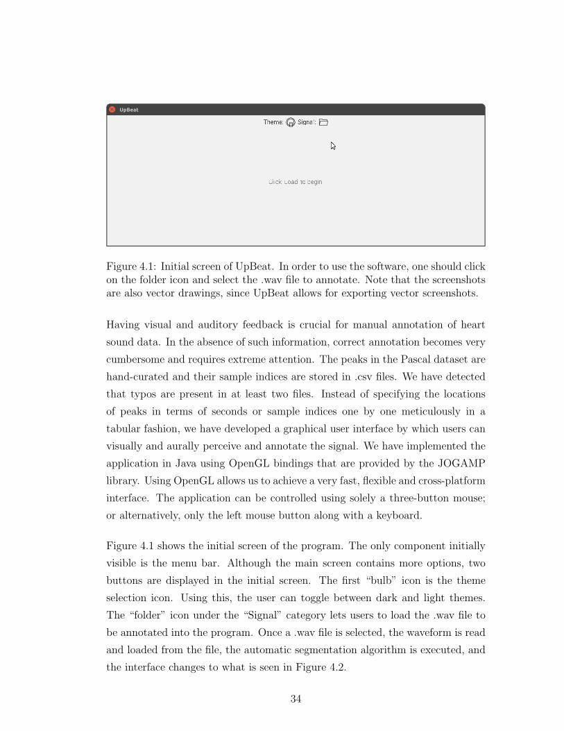
Figure 4.1: Initial screen of UpBeat. In order to use the software, one should clickon the folder icon and select the .wav file to annotate. Note that the screenshotsare also vector drawings, since UpBeat allows for exporting vector screenshots.
Having visual and auditory feedback is crucial for manual annotation of heart
sound data. In the absence of such information, correct annotation becomes very
cumbersome and requires extreme attention. The peaks in the Pascal dataset are
hand-curated and their sample indices are stored in .csv files. We have detected
that typos are present in at least two files. Instead of specifying the locations
of peaks in terms of seconds or sample indices one by one meticulously in a
tabular fashion, we have developed a graphical user interface by which users can
visually and aurally perceive and annotate the signal. We have implemented the
application in Java using OpenGL bindings that are provided by the JOGAMP
library. Using OpenGL allows us to achieve a very fast, flexible and cross-platform
interface. The application can be controlled using solely a three-button mouse;
or alternatively, only the left mouse button along with a keyboard.
Figure 4.1 shows the initial screen of the program. The only component initially
visible is the menu bar. Although the main screen contains more options, two
buttons are displayed in the initial screen. The first “bulb” icon is the theme
selection icon. Using this, the user can toggle between dark and light themes.
The “folder” icon under the “Signal” category lets users to load the .wav file to
be annotated into the program. Once a .wav file is selected, the waveform is read
and loaded from the file, the automatic segmentation algorithm is executed, and
the interface changes to what is seen in Figure 4.2.
34
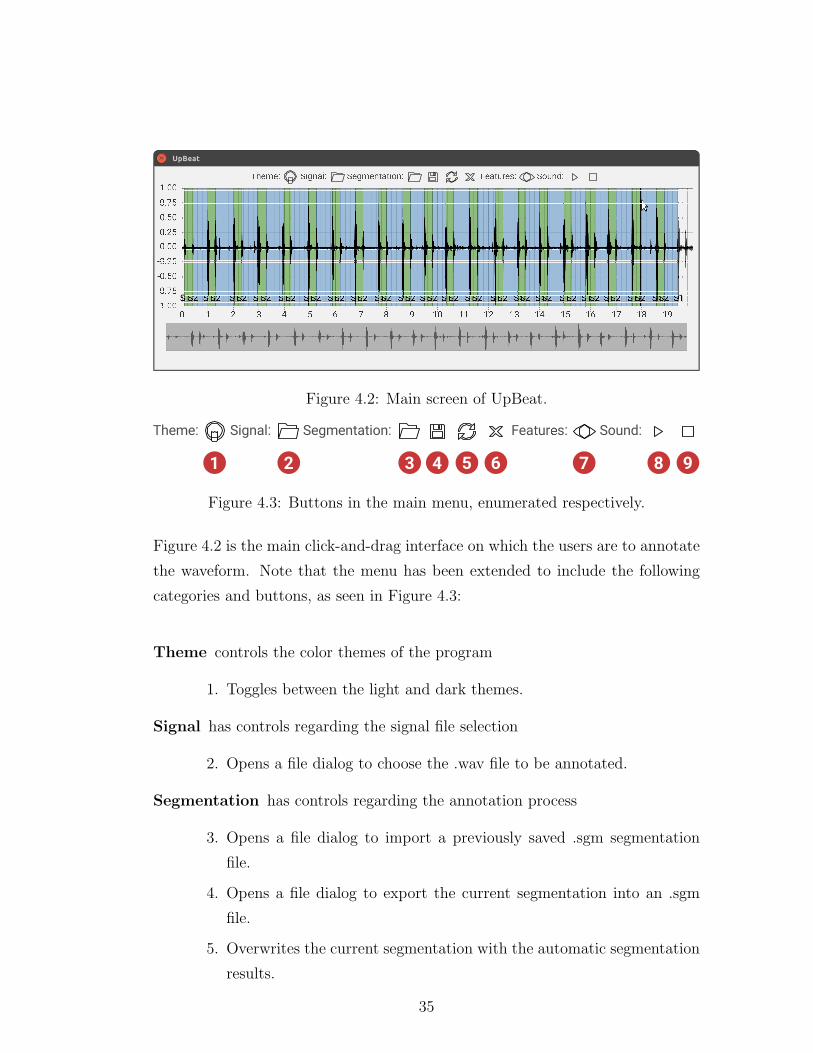
Figure 4.2: Main screen of UpBeat.
Figure 4.3: Buttons in the main menu, enumerated respectively.
Figure 4.2 is the main click-and-drag interface on which the users are to annotate
the waveform. Note that the menu has been extended to include the following
categories and buttons, as seen in Figure 4.3:
Theme controls the color themes of the program
1. Toggles between the light and dark themes.
Signal has controls regarding the signal file selection
2. Opens a file dialog to choose the .wav file to be annotated.
Segmentation has controls regarding the annotation process
3. Opens a file dialog to import a previously saved .sgm segmentation
file.
4. Opens a file dialog to export the current segmentation into an .sgm
file.
5. Overwrites the current segmentation with the automatic segmentation
results.
35

Figure 4.4: Dark theme.
6. Clears the segmentation for the user to start over.
Features has controls regarding feature selection
7. Shows/hides the feature display panel on the right.
Sound has controls regarding audio playback
8. Plays/pauses the heart sound recording
9. Stops the playback
Figure 4.4 shows the dark theme, which can be toggled from the first button in
the menu. At the very bottom of the window, hint texts regarding the menu
buttons that are hovered by the pointer are shown in the toolbar. Above that is
the zoom bar. The zoom bar allows the user to magnify a certain time interval
on the signal. The zoom bar shows the entire signal, on top of which a box
indicates the zoomed region. One can magnify a region of the signal by dragging
the handles of the zoom bar to cover that particular area. As the zoom bar is
modified, the large waveform in the middle of the screen will be updated to show
that particular region, as depicted in Figure 4.5.
Now that the signal in the middle is magnified, we can see the signal and the
peaks in more detail. The region shows a normalized version of the signal, where
the x-axis is marked to indicate seconds. Note that the signal is automatically
36

Figure 4.5: Zoom bar example. Notice how the waveform on the zoom bar showsthe entire signal, whereas the waveform rendered above is only the yellow sectionof the zoom bar.
segmented into sections and colored using blue and green. A green region depicts a
systolic interval; that is, between an S1 and the next S2. A blue region indicates
a diastolic interval, which is between an S2 and the following S1. An S2 - S2
interval is colored in red; whereas an S1 - S1 interval is not colored. Each of the
peaks is indicated with a vertical white line, and S1/S2 texts under them. Editing
peaks can be achieved with a 3-button mouse. Left-click adds an S1 peak (Shift
+ left-click adds an S2). Middle click converts an S1 to S2 (and vice versa). Right
click removes a peak. Existing peaks can also be dragged around. Alternatively,
Alt key + left-click serves as the middle click, in the absence of a middle mouse
button; and Ctrl + left-click simulates the right-click.
If the automatic segmentation algorithm works with few errors, as it generally
does; then a few minor corrections might be enough to complete the annotation
process. Otherwise, the cross sign on the menu bar can help reset the segmenta-
tion and start over (Figure 4.6).
The user might need to actually listen to the sound to properly annotate the
signal. After all, physicians are trained to auscultate and diagnose by ear. The
sound category in the menu allows the user to listen to the signal, and meanwhile
track the audio position visually. As shown in Figure 4.7, only the magnified
region is played in order to avoid confusion.
37

Figure 4.6: Using the clear button, the user can delete the segmentation so farand start over.
Figure 4.7: The play button allows the user to listen to the heart sound recording,and actually auscultate. The progress of the sound is depicted in the middle withthe yellow color, so that the physician can know the position of the audio.
38

Figure 4.8: The save button can be used for exporting the segmentation into an.sgm file. The user can load the segmentation and modify it later on using theload button on the left.
Once the segmentation is completed, it can be saved in an .sgm file. The format of
the file is minimalistic; the first value in the file is an integer; stating the number
of peaks in the file. The second value is also an integer, stating the number of
float fields in each peak. In our application, each peak is described by four values:
The first value is the location of the peak, in terms of milliseconds. The second
is the width of the peak; which is used by some segmentation algorithms. The
third feature is the amplitude of the peak. Finally, the fourth feature states the
type of the peak (S1 = 0, S2 = 1). All these four features are written as float
numbers to the .sgm with this order. The file format is extensible in the sense
that the user might choose to save more features than 4 for each peak. As long
as the first four features are not altered, all of the algorithms described in this
paper would work without any problem. Users can export their segmentations to
.sgm files using the Save button in the Segmentation category as shown in Figure
4.8
UpBeat also has a simple feature display tool, which finds the valid S1 - S2 -
S1 subchains in the segmentation, and draws these intervals by warping them
such that the systolic periods will overlap. The average of the energies of all
such available beats are then used for calculating 32 equidistant features, which
are then shown in the feature display window. The feature display tool can be
toggled using the eye icon as shown in Figure 4.9. This allows the user to intuit
39

Figure 4.9: The feature display tool, which provides an intuition about the cor-rectness of the segmentation.
how correct their segmentation process is. Any singular beat that is visibly off
can be observed.
We have also implemented a “quick segmentation” method, where the annotator
plays the sound and presses the Space key whenever they want to add a peak to
the position of yellow progress bar (which indicates the position of the playback).
If the previous peak is S1, the following peak will be added as an S2 and vice
versa. Furthermore, each of these peaks will immediately snap to the closest
largest sample in the data, so that they can properly show the positions of the
peaks. This was an experimental inclusion for Prof. Dr. Ali Oto to use, and is
not visible on the menu; however it remains fully functional.
UpBeat is capable of creating, loading, editing and saving a segmentation scheme
using a set of helpful features, and is capable of calculating and displaying the
average time-domain features of the cardiac cycle. Among the features of our pro-
gram is the playback of the sound, automatic segmentation of the signal; easy-to-
use interface for manual segmentation, and finally an advanced zoom mechanism
that allows detailed analysis of portions to be segmented. The presented tool can
be used to create a ground truth for heart sound segmentation. It is a starting
medium for other researchers to expand on what is available.
40

Chapter 5
Implementation of the Heart
Sound Segmentation Algorithms
As previously discussed, the majority of the work in the literature follows a pat-
tern that can be separated into six sequential steps, and the variation between
different PCG segmentation papers originate from their selection of methods in
each of these six steps.
Comparison of these methods as they are given in the literature would be incom-
plete. An approach taken in Part 1 by Method X might have been very useful
to be used with Method Y in Part 2. We compared every combination of all the
methods discussed in Chapter 3, also including novel ideas in several steps. In to-
tal, we tested more than 240 variations. Naturally, not all of these combinations
are meaningful, as to be seen empirically.
5.1 Algorithms
We have implemented several algorithms, including a majority of the work in the
literature. At several steps, we have our own contributions. We also implemented
41

other approaches such as MMR.
5.1.1 The Generic 6-Step Algorithm
The steps of the 6-step approach described in the related work are implemented
as follows.
5.1.1.1 Preprocessing
All the inputs of the program are re-sampled to a frequency of 4410 Hz, and then
normalized, such that the amplitude of the signal is scaled between -1 and 1. It
has been shown that this works better than the statistical normalization in our
case [23].
5.1.1.2 Time-frequency Transform
For the time-frequency transform step; STFT, Constant Q-transform,
Daubechies-4 wavelet and band pass filter are implemented. The FFT size for
the STFT scheme is set to 256, where the window function is selected as
w[n] =1− cos(2πn/256)
2
For the D4 wavelet, we consider d7, d6, d5 and a5 bands; which correspond to
the frequency bands 34.45 - 68.90 Hz, 68.90 - 137.81 Hz, 137.81 - 275.63 Hz, and
0 - 137.81 Hz, respectively. Hedayioglu and Liang et al. use d4, d5 and a4 bands;
which correspond to the 138 - 275 Hz, 69 - 138 Hz and 0-138 Hz bands with their
sampling frequency [6, 29].
Our contributions in this step are the Constant Q-transform and the band-pass
filter. The band-pass filter is designed to pass frequencies between 30 Hz and 60
Hz, using MATLAB’s fdatool. Since some approaches only considered the 45 Hz
42

band for segmentation; filtering the 30-60 Hz band makes sense.
Constant-Q transform was implemented as described by Brown [45]. Short-time
approach for time-frequency analysis is implemented, also the output is modified
to return the absolute value instead of complex output. We divide the 32 - 64
Hz band into 8 bins, therefore Q = 1/(2(1/8)− 1) ≈ 11. We empirically found out
that these parameters provide a sharp representation of S1 and S2 sounds.
5.1.1.3 Rectification and Envelope Detection
Absolute value, energy, Shannon energy and Shannon entropy are implemented
as is. Since envelogram and homomorphic filter provide very similar results, only
envelogram is implemented.
5.1.1.4 Thresholding and Merging Peaks
Both methodologies proposed by Gupta et al. and Hedayioglu [6, 23] are im-
plemented. The approach that Liang et al. proposed is very similar to that of
Hedayioglu, the only difference is the peak classification. We implemented our
own peak classification method that outperform these.
At each step, we also consider the case where that step is omitted. The total
number of combinations is 240; as depicted in Figure 5.1.
5.1.2 MMR
We have also proposed another approach that does not follow the regular algorith-
mic framework. The idea behind this approach is that we want to find the highest
peaks in the rectified signal, assuming that these peaks represent the S1 and S2
sounds (Note that the regular threshold method also makes the assumption that
these sounds have high amplitudes).
43
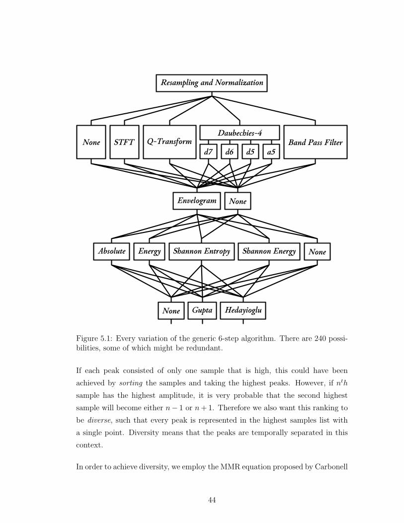
Figure 5.1: Every variation of the generic 6-step algorithm. There are 240 possi-bilities, some of which might be redundant.
If each peak consisted of only one sample that is high, this could have been
achieved by sorting the samples and taking the highest peaks. However, if nth
sample has the highest amplitude, it is very probable that the second highest
sample will become either n− 1 or n+1. Therefore we also want this ranking to
be diverse, such that every peak is represented in the highest samples list with
a single point. Diversity means that the peaks are temporally separated in this
context.
In order to achieve diversity, we employ the MMR equation proposed by Carbonell
44
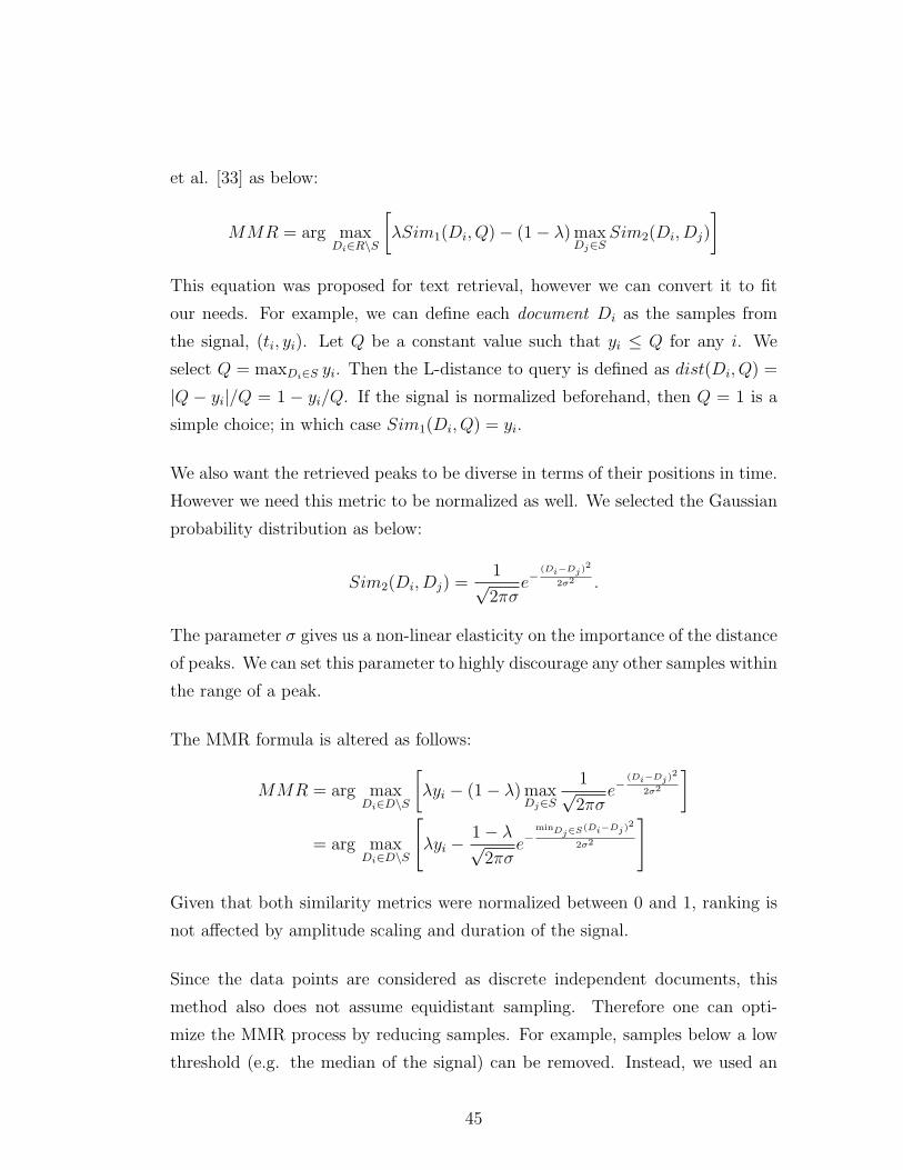
et al. [33] as below:
MMR = arg maxDi∈R\S
[
λSim1(Di, Q)− (1− λ) maxDj∈S
Sim2(Di, Dj)
]
This equation was proposed for text retrieval, however we can convert it to fit
our needs. For example, we can define each document Di as the samples from
the signal, (ti, yi). Let Q be a constant value such that yi ≤ Q for any i. We
select Q = maxDi∈S yi. Then the L-distance to query is defined as dist(Di, Q) =
|Q − yi|/Q = 1 − yi/Q. If the signal is normalized beforehand, then Q = 1 is a
simple choice; in which case Sim1(Di, Q) = yi.
We also want the retrieved peaks to be diverse in terms of their positions in time.
However we need this metric to be normalized as well. We selected the Gaussian
probability distribution as below:
Sim2(Di, Dj) =1√2πσ
e−(Di−Dj)
2
2σ2 .
The parameter σ gives us a non-linear elasticity on the importance of the distance
of peaks. We can set this parameter to highly discourage any other samples within
the range of a peak.
The MMR formula is altered as follows:
MMR = arg maxDi∈D\S
[
λyi − (1− λ) maxDj∈S
1√2πσ
e−(Di−Dj)
2
2σ2
]
= arg maxDi∈D\S
[
λyi −1− λ√2πσ
e−minDj∈S(Di−Dj)
2
2σ2
]
Given that both similarity metrics were normalized between 0 and 1, ranking is
not affected by amplitude scaling and duration of the signal.
Since the data points are considered as discrete independent documents, this
method also does not assume equidistant sampling. Therefore one can opti-
mize the MMR process by reducing samples. For example, samples below a low
threshold (e.g. the median of the signal) can be removed. Instead, we used an
45

elimination process where the taken samples are supposed to be the local maxima
in their 1-neighborhood, similar to how 1D SIFT algorithm detects key points
[50].
MMR is an iterative process; therefore requires the number of peaks to be detected
(k). Also, λ should be specified in advance. We added an extra parameter called
∆. The iterations are continued as long as there is at least one interval greater
than ∆, or the number of added peaks is less than k. Using 2-fold cross-validation,
we detected that λ = 0.5, σ = 120 ms, ∆ = 375 ms, k = tN/200 ms are optimal.
This is meaningful biologically, since 120 ms is the widest a peak can be [23]; and
2k = 400 ms is a feasible mean length for periods.
46
Chapter 6
Evaluation and Conclusion
6.1 Dataset
In order to test our methods, we used the Pascal heart sound classification chal-
lenge dataset [1].
Pascal dataset consists of two subsets, called Dataset A and Dataset B. Dataset
A is classified into four subcategories named ‘normal’, ‘murmur’, ‘extra heart
sound’ and ‘artifact’; whereas Dataset B consists of three classes named as ‘nor-
mal’, ‘murmur’ and ‘extrasystole’. Although the total number of recordings in
the dataset is 862; only the recordings in the ‘normal’ category has segmenta-
tion information for us to use as ground truth during evaluation. We have also
eliminated two segmentation schemes, because they had typos in the file that
corresponded to invalid segmentation schemes. Finally, any file with a duration
less than 2 seconds has been discarded, since most of the methods to be compared
require at least a few beats so that statistical parameters make sense. In the end
we are left with 66 reliable files.
47

6.2 Evaluation
All methods listed in the previous chapter are tested on the reduced dataset.
Although there are evaluation techniques proposed in the literature, most of
these metrics do not handle the case where the numbers of detected peaks to
not match. For instance, below is the evaluation metric required by the Pascal
challenge [1]:
δk =
Nk/2∑
i=1
(|RS1i − TS1i|+ |RS2i − TS2i|)
Nk
where δk is the average distance of the kth recording in the dataset, Nk is the total
number of peaks in the ground truth, RS1i (RS2i) are the locations of S1 (S2)
peaks of the ith heartbeat in the ground truth, TS1i (TS2i) are the locations of
S1 (S2) peaks in the calculated segmentation. The total error of the algorithm
on the entire dataset of N documents is calculated as
δ =N∑
j=0
δj.
The assumption inherent in this scheme is that all peaks in the ground truth have
corresponding peaks in the calculated segmentation. This may not be the case if
several peaks are missed (Type-II error), or if extra peaks are included (Type-I
error). One implementation would be to match the closest peak of the same type
for every peak; however in that case making a Type-I error has no cost (since
there will be no extra peaks to match these peaks), whereas Type-II errors will
have a distance longer than a beat can be. This is also not desired, because a
missing peak might not be a big problem for the classification algorithm that will
follow. Reversing the order in which we check the integrity of the peaks does not
help either. Below are several evaluation metrics we propose.
48
6.2.1 Method 1
We have proposed a more strict evaluation approach as follows. For every S1-S2-
S1 sub-chain (‘beat’) in the ground truth segmentation, let the temporal locations
of these peaks be ti−1, ti and ti+1. The calculated segmentation scheme is said to
have this beat if and only if all the following conditions hold:
1. There exists exactly one S1 peak t′i−1 within the range [ti−1 − τ, ti−1 + τ ].
2. There exists no S2 peaks within this range.
3. There exists exactly one S1 peak t′i+1 within the range [ti+1 − τ, ti+1 + τ ].
4. There exists no S2 peaks within this range.
5. There exists exactly one S2 peak t′i within the range [t′i−1, t′i+1].
6. There exists no S1 peaks within this range.
If all of these conditions are satisfied, the beat is said to have been detected by
the algorithm. The number of the detected beats is then divided to the number
of beats in the ground truth, which gives us an accuracy score, where the greater
value is better. Our tests revealed that τ = 50 ms provides a distinguishing
ranking, which also makes sense since a peak may have a width of 100 ms. An
example to how these rules work is depicted in Figure 6.1.
6.2.2 Method 2
Although the first evaluation method we propose is more to-the-point in that it
directly evaluates the ratio of cardiac cycles we correctly annotate; the discrete
nature of it requires another more sensitive evaluation metric. For example,
consider two segmentation algorithms. For each ground truth peak pi at t = ti,
let the first algorithm A1 annotate a peak at t = ti + 30 ms, and the second
algorithm A2 annotate a peak at t = ti− 4 ms. Assume the type of peak (S1/S2)
49

Figure 6.1: Several cases which involves the first evaluation metric. S1 peaksare described with lines with circles on them, and S2 lines have diamonds. Thedashed lines represent the τ neighborhood of the S1 peaks. Of all the cases above,only the first (topmost) is considered a valid (detected) beat.
is correct for all peaks in both A1 and A2. Since both algorithms generate unique
peaks within the 50 ms range of the ground truth, both will have a score of 1.0.
However, in reality A2 consistently produces closer results to the ground truth. It
can be argued that the first metric fails to differentiate between these two cases.
For this purpose we suggest a second evaluation metric as follows.
Since the intervals between an S1 and the following S2 is a systolic period, and
the interval between an S2 and the following S1 peak is a diastolic, and these
two regions never overlap; one can separate the time domain of a heart sound
signal into two subsets as S and D, respectively. The time domain is separated
by the ground truth into two such subsets as SG and DG, whereas the same
time domain is divided into SC and DC by the calculated peaks. If these regions
perfectly overlap, then segmentation is 100% successful.
Let SS = |SG ∩ SC |, DD = |DG ∩DC |, SD = |SG ∩DC |, and DS = |DG ∩ SC |.These four parameters represent the cardinalities (in this case, total lengths) of
regions, respectively, in which:
50
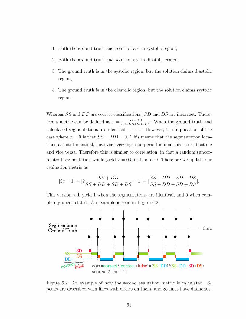
1. Both the ground truth and solution are in systolic region,
2. Both the ground truth and solution are in diastolic region,
3. The ground truth is in the systolic region, but the solution claims diastolic
region,
4. The ground truth is in the diastolic region, but the solution claims systolic
region.
Whereas SS andDD are correct classifications, SD andDS are incorrect. There-
fore a metric can be defined as x = SS+DDSS+DD+SD+DS
. When the ground truth and
calculated segmentations are identical, x = 1. However, the implication of the
case where x = 0 is that SS = DD = 0. This means that the segmentation loca-
tions are still identical, however every systolic period is identified as a diastolic
and vice versa. Therefore this is similar to correlation, in that a random (uncor-
related) segmentation would yield x = 0.5 instead of 0. Therefore we update our
evaluation metric as
|2x− 1| = |2 SS +DD
SS +DD + SD +DS− 1| = |SS +DD − SD −DS
SS +DD + SD +DS|.
This version will yield 1 when the segmentations are identical, and 0 when com-
pletely uncorrelated. An example is seen in Figure 6.2.
Figure 6.2: An example of how the second evaluation metric is calculated. S1
peaks are described with lines with circles on them, and S2 lines have diamonds.
51
6.2.3 Method 3
We have also developed a third metric that makes use of the Hungarian algorithm
to assign calculated peaks to the ground truth peaks. For n ground truth peaks
and m calculated peaks; we construct an n×m distance matrixM , such that mij
has the distance between ith ground truth peak and jth calculated peak (that is,
mij = ti − t′j). Then we try to assign ground truth peaks and calculated peaks
to each other, such that the total distance is minimized. This means that we
are trying to assign every calculated peak to the closest ground truth peak; and
this corresponds to picking min{n,m} elements from M that minimizes their
total with the condition that at most one element is selected from every row and
column. This is an NP-complete problem and can be solved using the Hungarian
algorithm. The summation can then be divided by the number of peaks to provide
a score. Unlike the two previous scores, in Method 3 the smaller score is better.
However, there are some problems with this approach. The fact that in the
ground truth dataset the annotations are not ‘snapped’ to the maximum samples
of each peak, but rather is placed at the beginning of each peak, means that the
best algorithm might not have the smallest error. Over-optimizing the similarity
in this fashion might be (and as we will see in the Results section, is) erroneous.
6.3 Results
The methods listed in Chapter 5 are tested on a valid subset of the Pascal heart
sound challenge dataset [1]. There were 66 normal heart sound recordings in
Dataset A and Dataset B combined with a valid annotation, full segmentation
and a duration longer than 3 seconds. This limitation on the file duration is
required since most of the methods do not work on very short files, which consist
of very few segments. Also, several files were not completely segmented, which
would mean that the evaluation quality would be reduced due to an erroneous
ground truth dataset. Such files were also excluded. Finally, annotations of two
heart sound files had errors. Excluding all these files, we ended up with a reliable
52
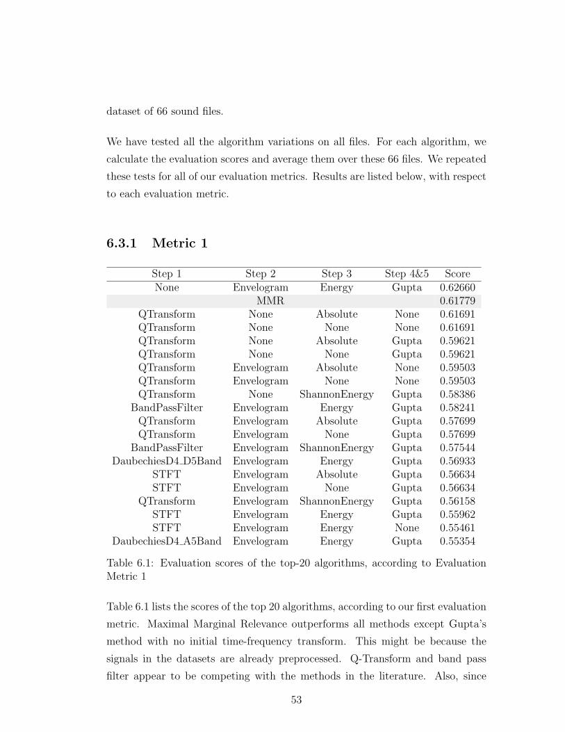
dataset of 66 sound files.
We have tested all the algorithm variations on all files. For each algorithm, we
calculate the evaluation scores and average them over these 66 files. We repeated
these tests for all of our evaluation metrics. Results are listed below, with respect
to each evaluation metric.
6.3.1 Metric 1
Step 1 Step 2 Step 3 Step 4&5 ScoreNone Envelogram Energy Gupta 0.62660
MMR 0.61779QTransform None Absolute None 0.61691QTransform None None None 0.61691QTransform None Absolute Gupta 0.59621QTransform None None Gupta 0.59621QTransform Envelogram Absolute None 0.59503QTransform Envelogram None None 0.59503QTransform None ShannonEnergy Gupta 0.58386
BandPassFilter Envelogram Energy Gupta 0.58241QTransform Envelogram Absolute Gupta 0.57699QTransform Envelogram None Gupta 0.57699
BandPassFilter Envelogram ShannonEnergy Gupta 0.57544DaubechiesD4 D5Band Envelogram Energy Gupta 0.56933
STFT Envelogram Absolute Gupta 0.56634STFT Envelogram None Gupta 0.56634
QTransform Envelogram ShannonEnergy Gupta 0.56158STFT Envelogram Energy Gupta 0.55962STFT Envelogram Energy None 0.55461
DaubechiesD4 A5Band Envelogram Energy Gupta 0.55354
Table 6.1: Evaluation scores of the top-20 algorithms, according to EvaluationMetric 1
Table 6.1 lists the scores of the top 20 algorithms, according to our first evaluation
metric. Maximal Marginal Relevance outperforms all methods except Gupta’s
method with no initial time-frequency transform. This might be because the
signals in the datasets are already preprocessed. Q-Transform and band pass
filter appear to be competing with the methods in the literature. Also, since
53

our implementation of Q-Transform reduces the number of samples taken (due
to high computational cost), envelogram becomes a redundant step.
6.3.2 Metric 2
Table 6.2 lists the scores of the top 20 algorithms with respect to our second
evaluation metric. Maximal Marginal Relevance outperforms all other methods.
The following four methods are also the Top-4 results for the first metric. Again,
Q-Transform without envelogram produces competitive results.
Step 1 Step 2 Step 3 Step 4&5 ScoreMMR 0.62383
None Envelogram Energy Gupta 0.61765QTransform None Absolute None 0.58738QTransform None None None 0.58738
BandPassFilter Envelogram ShannonEnergy Gupta 0.58497BandPassFilter Envelogram Energy Gupta 0.57260QTransform None ShannonEnergy Gupta 0.57005
None Envelogram ShannonEnergy Gupta 0.56909QTransform Envelogram Absolute None 0.56585QTransform Envelogram None None 0.56585
DaubechiesD4 A5Band Envelogram Energy Gupta 0.56577QTransform None Absolute Gupta 0.56332QTransform None None Gupta 0.56332
STFT Envelogram Energy Gupta 0.54927STFT Envelogram Absolute Gupta 0.54921STFT Envelogram None Gupta 0.54921
QTransform Envelogram Absolute Gupta 0.54908QTransform Envelogram None Gupta 0.54908
BandPassFilter Envelogram Absolute Gupta 0.54320STFT Envelogram Energy None 0.54087
Table 6.2: Evaluation scores of the top-20 algorithms, according to EvaluationMetric 2
54
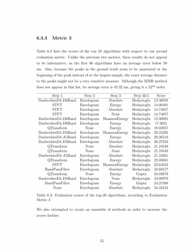
6.3.3 Metric 3
Table 6.3 lists the scores of the top 20 algorithms with respect to our second
evaluation metric. Unlike the previous two metrics, these results do not appear
to be informative; as the first 86 algorithms have an average error below 50
ms. Also, because the peaks in the ground truth seem to be annotated at the
beginning of the peak instead of at the largest sample, the exact average distance
to the peaks might not be a very sensitive measure. Although the MMR method
does not appear in this list, its average error is 35.32 ms, giving it a 52nd order.
Step 1 Step 2 Step 3 Step 4&5 ScoreDaubechiesD4 D6Band Envelogram Absolute Hedayioglu 13.36058
STFT Envelogram Energy Hedayioglu 14.00491STFT Envelogram Absolute Hedayioglu 14.74057STFT Envelogram None Hedayioglu 14.74057
DaubechiesD4 D6Band Envelogram ShannonEnergy Hedayioglu 15.90085DaubechiesD4 D6Band Envelogram Energy Hedayioglu 17.9021
QTransform None Energy Hedayioglu 18.02057DaubechiesD4 D5Band Envelogram ShannonEnergy Hedayioglu 20.25292DaubechiesD4 A5Band Envelogram Energy Hedayioglu 20.26519DaubechiesD4 D5Band Envelogram Absolute Hedayioglu 20.27933
QTransform None Absolute Hedayioglu 21.10549QTransform None None Hedayioglu 21.10549
DaubechiesD4 A5Band Envelogram Absolute Hedayioglu 21.24261QTransform Envelogram Energy Hedayioglu 22.03681
STFT Envelogram ShannonEnergy Hedayioglu 22.64943BandPassFilter Envelogram Absolute Hedayioglu 22.68577QTransform None Energy Gupta 24.02679
DaubechiesD4 D5Band Envelogram None Hedayioglu 24.08979BandPassFilter Envelogram Energy Gupta 24.21508
None Envelogram Absolute Hedayioglu 24.43124
Table 6.3: Evaluation scores of the top-20 algorithms, according to EvaluationMetric 3
We also attempted to create an ensemble of methods in order to increase the
scores further.
55
6.4 Ensemble
Although we have a ranking of methods, the scores obtained do not have statis-
tically significant advantage over each other. In order to achieve better perfor-
mance, we propose an ensemble of 24 methods. Table 6.4 lists the methods that
we picked for this ensemble.
We first calculated that if we had a perfect ensemble metric, such that for each
file we could perfectly select the best performing algorithm we have; then the
ensemble score would be 0.84 (according to the first evaluation score). This means
that although singular methods cannot exceed a score of 0.63, this is not an upper
limit enforced by the dataset, and there is significant room for improvement.
We attempted to use the standard deviation of the systolic and diastolic intervals
as an ensemble score, however this further reduces the ensemble score. Our final
metric is as follows:
To merge the methods, we count the number of S1 - S2 - S1 chains in the calculated
segmentation, and divide it to the total number of peaks. The segmentation
scheme with a higher ratio of such chains has a higher score. Whichever algorithm
has the highest score for a given file is selected as the answer, and presented
as the outcome of the ensemble. Our ensemble achieved a score of 0.75123,
outperforming any singular method. The same ensemble has an evaluation score
of 0.77259 according to the second metric.
The ensemble has a score of 37.460518 ms according to the third evaluation
metric, which is ‘worse’ than the top-20 methods. This strengthens our concerns
regarding the inefficiency of the third metric.
56

Step 1 Step 2 Step 3 Step 4&5STFT Envelogram Absolute Gupta
QTransform Envelogram Absolute GuptaDaubechiesD4 D6Band Envelogram Absolute GuptaDaubechiesD4 D5Band Envelogram Absolute GuptaDaubechiesD4 A5Band Envelogram Absolute Gupta
BandPassFilter Envelogram Absolute GuptaNone Envelogram Absolute GuptaSTFT Envelogram Energy Gupta
DaubechiesD4 D6Band Envelogram Energy GuptaDaubechiesD4 D5Band Envelogram Energy Gupta
BandPassFilter Envelogram Energy GuptaNone Envelogram Energy Gupta
BandPassFilter Envelogram ShannonEntropy GuptaDaubechiesD4 D6Band Envelogram ShannonEnergy Gupta
BandPassFilter Envelogram ShannonEnergy GuptaDaubechiesD4 D5Band Envelogram None Gupta
STFT None Absolute GuptaNone Envelogram Absolute HedayiogluSTFT Envelogram ShannonEntropy Hedayioglu
DaubechiesD4 D6Band Envelogram ShannonEntropy HedayiogluDaubechiesD4 A5Band Envelogram ShannonEnergy Hedayioglu
STFT None ShannonEnergy HedayiogluNone Envelogram Energy None
MMR
Table 6.4: Methods selected for the ensemble
6.5 Conclusion
In this work we have investigated the topic of heart sound segmentation. The
literature on cardiac analysis lacks the unification of results on a common data set
with properly defined evaluation metrics. We have implemented, compared and
combined the majority of the work in the literature. We have also proposed sev-
eral additions on the generic 6-step segmentation algorithm, as well as introducing
the well-known Maximal Marginal Relevance equation on the segmentation prob-
lem. We introduced two evaluation measures which take into consideration the
Type-I and Type-II errors that can occur on segmentation. When tested with
the first evaluation metric, the maximal marginal relevance method outperforms
57

other algorithms, whereas the Constant-Q transform competes with other meth-
ods effectively. We also described a way of combining several methods in order
to increase performance. While the maximum score a singular method could
achieve was 0.63 (meaning that the 63 percent of heartbeats have been correctly
annotated with at most a 50 ms deviation from the ground truth), our ensemble
shows 0.75 accuracy. The second evaluation metric that we introduce provides
a similar ranking for the methods that we evaluate. In this case, the maximum
score belongs to the MMR algorithm (0.62), whereas the ensemble has a score of
0.77.
We also programmed an intuitive, easy-to-use standalone application that can
be used for manual heart sound segmentation to allow constructing ground truth
datasets, or provide a means of visualization that can help obtain an insight on the
heart sound waveform. The tests were performed on the 66 suitable files in Pascal
dataset. We propose as future work to extend the dataset for more reliable tests,
refine the ensemble method as empirical results show that there is more room for
performance improvement, and experiment with other time-frequency transform
methods such as SAX [51] and piecewise linear modeling [52] etc.
58
Bibliography
[1] P. Bentley, G. Nordehn, M. Coimbra, and S. Mannor, “The PAS-
CAL Classifying Heart Sounds Challenge 2011 (CHSC2011) Results.”
http://www.peterjbentley.com/heartchallenge/index.html, 2011.
[2] D. Venes, Taber’s cyclopedic medical dictionary. FA Davis, 2013.
[3] “Cardiovascular System at the US National Library of Medicine Medical
Subject Headings (MeSH).” http://goo.gl/G4xLvg, 2011.
[4] A. Alwan et al., Global status report on noncommunicable diseases 2010.
World Health Organization, 2011.
[5] World Health Organization, Noncommunicable Diseases (NCD) Country
Profiles. 2014.
[6] F. d. L. Hedayioglu, “Heart sound segmentation for digital stethoscope in-
tegration,” 2011.
[7] “Heart murmur - wikipedia, the free encyclopedia.”
[8] OkCopay, “National median costs of MRI scans.”
http://www.okcopay.com/results/mri-abdominal.
[9] T. T. Birligi, “Resmi saglık kurumları fiyat tarifesi.”
http://www.ttb.org.tr/mevzuat/2005ek/but/EK-82.htm, 2014.
[10] T. C. Lin, Phonocardiogram segmentation. PhD thesis, 2005.
59
[11] J. Vepa, “Classification of heart murmurs using cepstral features and support
vector machines,” in Engineering in Medicine and Biology Society, 2009.
EMBC 2009. Annual International Conference of the IEEE, pp. 2539–2542,
IEEE, 2009.
[12] S. Jabbari and H. Ghassemian, “Modeling of heart systolic murmurs based
on multivariate matching pursuit for diagnosis of valvular disorders,” Com-
puters in biology and medicine, vol. 41, no. 9, pp. 802–811, 2011.
[13] E. Delgado-Trejos, A. Quiceno-Manrique, J. Godino-Llorente, M. Blanco-
Velasco, and G. Castellanos-Dominguez, “Digital auscultation analysis for
heart murmur detection,” Annals of biomedical engineering, vol. 37, no. 2,
pp. 337–353, 2009.
[14] C. G. DeGroff, S. Bhatikar, J. Hertzberg, R. Shandas, L. Valdes-Cruz, and
R. L. Mahajan, “Artificial neural network–based method of screening heart
murmurs in children,” Circulation, vol. 103, no. 22, pp. 2711–2716, 2001.
[15] S. L. Strunic, F. Rios-Gutierrez, R. Alba-Flores, G. Nordehn, and S. Burns,
“Detection and classification of cardiac murmurs using segmentation tech-
niques and artificial neural networks,” in Computational Intelligence and
Data Mining, 2007. CIDM 2007. IEEE Symposium on, pp. 397–404, IEEE,
2007.
[16] Z. Syed, D. Leeds, D. Curtis, F. Nesta, R. A. Levine, and J. Guttag, “A
framework for the analysis of acoustical cardiac signals,” Biomedical Engi-
neering, IEEE Transactions on, vol. 54, no. 4, pp. 651–662, 2007.
[17] C. Ahlstrom, P. Hult, P. Rask, J.-E. Karlsson, E. Nylander, U. Dahlstrom,
and P. Ask, “Feature extraction for systolic heart murmur classification,”
Annals of biomedical engineering, vol. 34, no. 11, pp. 1666–1677, 2006.
[18] F. Javed and P. Venkatachalam, “A signal processing module for the analysis
of heart sounds and heart murmurs,” in Journal of Physics: Conference
Series, vol. 34, p. 1098, IOP Publishing, 2006.
60
[19] Y. Chen, S. Wang, C.-H. Shen, and F. K. Choy, “Matrix decomposition
based feature extraction for murmur classification,” Medical engineering &
physics, vol. 34, no. 6, pp. 756–761, 2012.
[20] A. Quiceno-Manrique, J. Godino-Llorente, M. Blanco-Velasco, and
G. Castellanos-Dominguez, “Selection of dynamic features based on time–
frequency representations for heart murmur detection from phonocardio-
graphic signals,” Annals of biomedical engineering, vol. 38, no. 1, pp. 118–
137, 2010.
[21] F. Wang, T. Syeda-Mahmood, and D. Beymer, “Finding disease similarity by
combining ecg with heart auscultation sound,” in Computers in Cardiology,
2007, pp. 261–264, IEEE, 2007.
[22] M. G. Johnson, A. Tewfik, K. Madhu, and A. G. Erdman, “Using voice-
recognition technology to eliminate cardiac cycle segmentation in automated
heart sound diagnosis,” Biomedical Instrumentation & Technology, vol. 41,
no. 2, pp. 157–166, 2007.
[23] C. N. Gupta, R. Palaniappan, S. Swaminathan, and S. M. Krishnan, “Neural
network classification of homomorphic segmented heart sounds,” Applied
Soft Computing, vol. 7, no. 1, pp. 286–297, 2007.
[24] H. N. Liang et al., “A feature extraction algorithm based on wavelet packet
decomposition for heart sound signals,” Time-Frequency and Time-Scale
Analysis, 1998. Proceedings of the IEEE-SP International Symposium on,
1998.
[25] G. Livanos, N. Ranganathan, and J. Jiang, “Heart sound analysis using the
s transform,” in Computers in Cardiology 2000, pp. 587–590, IEEE, 2000.
[26] O. Abdel-Alim, N. Hamdy, and M. El-Hanjouri, “Heart diseases diagnosis
using heart sounds,” in Radio Science Conference, 2002.(NRSC 2002). Pro-
ceedings of the Nineteenth National, pp. 634–640, IEEE, 2002.
[27] M. W. Groch, J. R. Domnanovich, and W. D. Erwin, “A new heart-sounds
gating device for medical imaging,” Biomedical Engineering, IEEE Transac-
tions on, vol. 39, no. 3, pp. 307–310, 1992.
61

[28] A. Haghighi-Mood and J. Torry, “A sub-band energy tracking algorithm for
heart sound segmentation,” in Computers in Cardiology 1995, pp. 501–504,
IEEE, 1995.
[29] H. Liang, S. Lukkarinen, and I. Hartimo, “Heart sound segmentation algo-
rithm based on heart sound envelogram,” in Computers in Cardiology 1997,
pp. 105–108, IEEE, 1997.
[30] A. C. Stasis, E. Loukis, S. Pavlopoulos, and D. Koutsouris, “Using deci-
sion tree algorithms as a basis for a heart sound diagnosis decision support
system,” in Information Technology Applications in Biomedicine, 2003. 4th
International IEEE EMBS Special Topic Conference on, pp. 354–357, IEEE,
2003.
[31] S. Choi and Z. Jiang, “Comparison of envelope extraction algorithms for car-
diac sound signal segmentation,” Expert Systems with Applications, vol. 34,
no. 2, pp. 1056–1069, 2008.
[32] A. Mondal, P. Bhattacharya, and G. Saha, “An automated tool for localiza-
tion of heart sound components s1, s2, s3 and s4 in pulmonary sounds using
hilbert transform and heron’s formula,” SpringerPlus, vol. 2, no. 1, pp. 1–14,
2013.
[33] J. Carbonell and J. Goldstein, “The use of mmr, diversity-based reranking for
reordering documents and producing summaries,” in Proceedings of the 21st
annual international ACM SIGIR conference on Research and development
in information retrieval, pp. 335–336, ACM, 1998.
[34] S. K. Mitra and Y. Kuo, Digital signal processing: a computer-based ap-
proach, vol. 2. McGraw-Hill New York, 2006.
[35] A. E. Cetin, “Lecture notes on discrete-time signal processing.”
http://kilyos.ee.bilkent.edu.tr/~ee424/EE424.pdf, 2012. [Online;
accessed 7-May-2015].
[36] J. Allen, “Short term spectral analysis, synthesis, and modification by dis-
crete fourier transform,” Acoustics, Speech and Signal Processing, IEEE
Transactions on, vol. 25, pp. 235–238, Jun 1977.
62

[37] C. K. Chui, An introduction to wavelets, vol. 1. Academic press, 2014.
[38] I. Daubechies et al., Ten lectures on wavelets, vol. 61. SIAM, 1992.
[39] L. Chun-Lin, “A tutorial of the wavelet transform,” NTUEE, Taiwan, 2010.
[40] R. G. Stockwell, L. Mansinha, and R. Lowe, “Localization of the com-
plex spectrum: the s transform,” Signal Processing, IEEE Transactions on,
vol. 44, no. 4, pp. 998–1001, 1996.
[41] R. A. Brown and R. Frayne, “A fast discrete s-transform for biomedical signal
processing,” in Engineering in Medicine and Biology Society, 2008. EMBS
2008. 30th Annual International Conference of the IEEE, pp. 2586–2589,
IEEE, 2008.
[42] S. Mallat, A wavelet tour of signal processing. Academic press, 1999.
[43] A. Alhazred, “The Necronomicon (Al Azif).”
[44] J. C. Brown and M. S. Puckette, “An efficient algorithm for the calculation
of a constant q transform,” The Journal of the Acoustical Society of America,
vol. 92, no. 5, pp. 2698–2701, 1992.
[45] J. C. Brown, “Calculation of a constant q spectral transform,” The Journal
of the Acoustical Society of America, vol. 89, no. 1, pp. 425–434, 1991.
[46] N. Baddour, “Heart Signal Recordings - Invitro and Invivo,” 04 2014.
[47] A. Gharehbaghi, T. Dutoit, A. Sepehri, P. Hult, and P. Ask, “An automatic
tool for pediatric heart sounds segmentation,” in Computing in Cardiology,
2011, pp. 37–40, IEEE, 2011.
[48] E. F. Gomes, A. M. Jorge, and P. J. Azevedo, “Classifying heart sounds
using multiresolution time series motifs: an exploratory study,” in Proceed-
ings of the International C* Conference on Computer Science and Software
Engineering, pp. 23–30, ACM, 2013.
63
[49] A. Castro, T. T. Vinhoza, S. S. Mattos, and M. T. Coimbra, “Heart sound
segmentation of pediatric auscultations using wavelet analysis,” in Engi-
neering in Medicine and Biology Society (EMBC), 2013 35th Annual Inter-
national Conference of the IEEE, pp. 3909–3912, IEEE, 2013.
[50] D. G. Lowe, “Distinctive image features from scale-invariant keypoints,”
International journal of computer vision, vol. 60, no. 2, pp. 91–110, 2004.
[51] J. Lin, E. Keogh, S. Lonardi, and B. Chiu, “A symbolic representation of
time series, with implications for streaming algorithms,” in Proceedings of
the 8th ACM SIGMOD workshop on Research issues in data mining and
knowledge discovery, pp. 2–11, ACM, 2003.
[52] M. Johansson, “Piecewise linear modeling,” in Piecewise Linear Control Sys-
tems, pp. 9–31, Springer, 2003.
64


![Audio Fundamentals - 法政大学 [HOSEI UNIVERSITY]cis.k.hosei.ac.jp/~jianhua/course/mm/Lesson02.pdf · Audio Fundamentals • Sound, Sound Wave and Sound Perception • Sound Signal](https://img.dokumen.tips/doc/110x75/5a7da5f67f8b9a49588dbb77/audio-fundamentals-hosei-universityciskhoseiacjpjianhuacoursemm.jpg)


