Embed Size (px)
Citation preview

Healthcare Exceptionalism? Performance andAllocation in the U.S. Healthcare Sector
Amitabh Chandra, Amy Finkelstein, Adam Sacarny and Chad Syverson∗
January 2016
Abstract
The conventional wisdom in health economics is that idiosyncratic features of
the healthcare sector leave little scope for market forces to allocate consumers to
higher performance producers. However, we find robust evidence across a variety of
conditions and performance measures that higher quality hospitals tend to have higher
market shares at a point in time and to expand more over time. Moreover, we find that
the relationship between performance and allocation is stronger among patients who
have greater scope for hospital choice, suggesting a role for demand in allocation in
the hospital sector. Our findings suggest that the healthcare sector may have more
in common with “traditional” sectors subject to standard market forces than is often
assumed.
JEL classification: D22, D24, I11
Keywords: Hospital Performance; Allocation; Healthcare
∗Chandra: Harvard Kennedy School and NBER, [email protected]; Finkelstein: Depart-ment of Economics, MIT and NBER; [email protected]; Sacarny: Department of Health Policy and Manage-ment, Columbia University Mailman School of Public Health, [email protected]; Syverson: ChicagoBooth and NBER; [email protected] are grateful to Daron Acemoglu, Nick Bloom, Iain Cockburn, Chris Conlon, Angus Deaton, MarkDuggan, Joe Doyle, Liran Einav, Matthew Gentzkow, Michael Greenstone, Jonathan Gruber, Ben Olken,Jonathan Skinner, Doug Staiger, Scott Stern, Heidi Williams, numerous seminar participants, four ref-erees, and the Editor for helpful comments and advice, and to Maurice Dalton and Nivedhitha Sub-ramanian for expert research assistance. We gratefully acknowledge funding from the National Insti-tute on Aging: P01 AG005842 and P01 AG019783 (Chandra), R01 AG032449 (Finkelstein) and T32-AG000186 (Sacarny). Finkelstein, Sacarny, and Syverson declare that they have no relevant or mate-rial financial interests that relate to the research described in this paper. Chandra reports serving onthe Congressional Budget Office (CBO) Panel of Health Advisors. Other disclosures are available athttps://www.hks.harvard.edu/about/faculty-staff-directory/amitabh-chandra
1

I Introduction
A classic “signpost of competition” in manufacturing industries is that higher pro-ductivity producers are allocated greater market share at a point in time and overtime. The conventional wisdom in the healthcare sector, however, is that idiosyn-cratic, institutional features of this sector dull or eliminate these competitive reallo-cation forces. Oft-cited culprits include consumers who lack knowledge of or timeto respond to the quality and price differences across providers, generous healthinsurance that insulates consumers from the direct financial consequences of theirhealthcare consumption decisions, and public sector reimbursement that provideslittle incentive for providers to achieve productive efficiency. These factors arewidely believed to dampen the disciplining force of demand-side competition thatexists in most other sectors.
This notion of “healthcare exceptionalism” has a long tradition in health eco-nomics. It dates back at least to the seminal article of Arrow (1963), which startedthe modern field of health economics by emphasizing key features of the healthcare industry that distinguish it from most other sectors and therefore warrant tai-lored study. Echoing and advancing the view that demand-side competition doesnot discipline healthcare providers, Cutler (2010) notes:
“[T]here are two fundamental barriers to organizational innovation inhealthcare. The first is the lack of good information on quality. Within amarket, it is difficult to tell which providers are high quality and whichare low quality. . . . Difficulty measuring quality also makes expansion
of high-quality firms more difficult. [emphasis added] . . . The secondbarrier is the stagnant compensation system of public insurance plans.”(p. 3)
In a similar vein, Skinner (2011) states in his overview article on regional variationsin healthcare:
“[Low productivity producers are] . . . unlikely to be shaken out by nor-mal competitive forces, given the patchwork of providers, consumersand third-party payers each of which faces inadequate incentives to im-prove quality or lower costs. . . ” (p. 47)
2

In this paper, we question this conventional wisdom by investigating empiricallywhether and to what extent higher performing hospitals tend to attract greater mar-ket share. We look at allocation of Medicare patients for several different healthconditions – heart attacks (called acute myocardial infarction, or AMI), congestiveheart failure, and pneumonia – and a common pair of surgical procedures – hip andknee replacements – that together account for almost one-fifth of Medicare hospitaladmissions and hospital spending. Hospital “performance” or “quality” (words thatwe use interchangeably) is, of course a highly multidimensional object. Broadlyspeaking, we think of hospital quality as increasing in hospital attributes that in-crease the utility of patients or their surrogates; hospital quality therefore includesthe ability of the hospital to generate good health outcomes, patient beliefs about thehospital’s ability to generate good health outcomes, and patient satisfaction with thehospital experience. In practice, we examine several different hospital quality mea-sures: clinical outcomes (survival and readmission), conformance with processes ofcare (i.e. adherence to well-established practice guidelines), and ex-post measuresof patients’ satisfaction with their experience (such as whether the room was quietand whether nurses communicated well).
We find robust evidence that higher performing hospitals – as defined either bythe health outcome-based measures or the process of care measures – tend to havegreater market share (i.e. more Medicare patients) at a point in time, and experiencemore growth in market share over time. This positive correlation between qualityand market share does not exist, however, when quality is measured by patient self-reported satisfaction with the hospital stay. Importantly, where we do find a positivecorrelation between quality and market share, these correlations are systematicallyand substantially stronger among patients who have more scope for choice. Specif-ically, within a condition the correlation between hospital quality and allocation isstronger for admissions that are transfers from other hospitals than admissions thatcome via the emergency room. We interpret these results as consistent with a rolefor consumer demand, either by patients or their surrogates, to affect the allocationof patients to hospitals. Also, consistent with consumer demand in a setting wherethere is little if any financial consequence of hospital choice for the patient, we findthat conditional on hospital performance, the market does not penalize hospitals
3

with higher inputs – if anything, it rewards them. The normative implications of thereallocation we observe therefore differ for the patient and for a benevolent socialplanner.
Qualitatively, our results reject the strong form of the healthcare exceptionalismhypothesis: that there are no forces allocating market share to higher quality hos-pitals. Quantitatively, they suggest an important role for these reallocation forces.For example, we find that reallocation to higher quality hospitals can explain abouta quarter of the 3.9 percentage point increase in 30-day survival for AMI over the1996-2008 period. In other words, AMI survival rates rose almost one percentagepoint over the period simply because patient flows shifted to higher-quality hospi-tals. For heart failure and pneumonia – where the secular improvements in survivalwere, respectively, 0.9 and 3.2 percentage points over this time period – we find asomewhat smaller contribution of reallocation of 18 percent and 6 percent.
The rest of the paper proceeds as follows. Section II describes the analyticalframework. Section III discusses our setting and data. Section IV presents our mainresults on the relationship between hospital quality and market share. Section Vpresents additional evidence consistent with a demand-based mechanism for theseallocation results. The last section concludes.
II Analytical Approach: Static and Dynamic Alloca-tion
Our primary empirical exercise examines the correlation between producer (i.e.hospital) performance and market share at a point in time, and the correlation be-tween producer performance and growth in market share over time. This relation-ship has been analyzed extensively in a variety of industries and countries as a proxyfor the role of competition in these settings (e.g. Olley and Pakes, 1996; Pavcnik,2002; Escribano and Guasch, 2005; Bartelsman, Haltiwanger and Scarpetta, 2013;Collard-Wexler and De Loecker, 2015). Intuitively, competitive forces exert pres-sure on lower productivity firms, causing them to either become more efficient,shrink, or exit.
4

Models of such reallocation mechanisms among heterogeneous-productivityproducers have found applications in a number of fields, including industrial or-ganization, trade, and macroeconomics.1 While these models differ considerablyin their specifics, they share a common intuition: greater competition – as re-flected in greater consumer willingness or ability to substitute to alternative pro-ducers – makes it more difficult for higher-cost, lower-productivity firms to earnpositive profits, since demand is more responsive to cost and price differentialsacross firms. As substitutability increases, purchases are reallocated to higher pro-ductivity providers, raising the correlation between productivity and market shareat a point in time (“static allocation”) and causing higher productivity providers toexperience more growth over time (“dynamic allocation”).
The literature to date has focused on the relationship between market share andproductivity, or the ratio of output to inputs. However, in the health care setting –and particularly for the Medicare enrollees that are the focus of this study – con-sumers bear little to none of the costs of production. As a result, it is more sensibleto view competition as occurring mainly over output “performance”, or quality,rather than productivity per se. In Appendix A we therefore present a model ofquality competition among firms that face consumers who are not sensitive to inputcosts. This model preserves the intuition that consumer ability or willingness tosubstitute across providers drives the relationship between performance and marketallocation. However, in a setting where, due to insurance, consumers have little orno financial stake in their selection, the market need not allocate away from firmsthat are higher cost for a given level of output.
For the static allocation analysis, we will use the following regression frame-work:
(1) ln(Nh) = βs0 +β
s1qh + γ
sM + ε
sh
where Nh is a measure of the market size of hospital h, γsM are market fixed ef-
fects, and qh is a measure of the quality of hospital h. Thus β s1 reflects the static
1See, for example, Ericson and Pakes (1995); Melitz (2003); and Asplund and Nocke (2006).
5

relationship between a hospital’s quality and its market share within a market. Ifthe coefficient is positive, as has been found with respect to productivity in manyU.S. manufacturing industries (e.g., Olley and Pakes, 1996; Hortaçsu and Syverson,2007; Bartelsman, Haltiwanger and Scarpetta, 2013), it indicates that higher perfor-mance producers have a greater share of activity at a point in time. If β s
1 is zero ornegative, it indicates that lower quality facilities are the same size or larger thantheir high quality counterparts and suggests that forces beyond quality competitionare driving the allocation of market activity. In the manufacturing productivity lit-erature, β s
1 ≤ 0 has been found in some former Soviet-bloc countries in the early1990s (Bartelsman, Haltiwanger and Scarpetta, 2013) and in the U.S. steel industrycirca 1960-70 (Collard-Wexler and De Loecker, 2015).2
The static allocation analysis in equation (1) can reflect the market’s ability toreallocate activity from low quality hospitals to higher quality ones, but it showsthe outcome of this process rather than the process itself. To measure the actualdynamics of the market’s selection and reallocation mechanisms, we examine therelationship between a hospital’s quality and its future growth. We will estimate:
(2) ∆h = βd0 +β
d1 qh + γ
dM + ε
dh
where ∆h is a measure of the hospital’s growth rate in admissions and all othervariables are defined as in equation (1). A positive correlation between quality andgrowth indicates that higher performance hospitals see larger gains in patient ad-missions, and points to the operation of a selection and reallocation process. Theproductivity literature has found widespread evidence in developed country manu-facturing and retail that higher productivity producers experience growth in marketshares (e.g. Scarpetta et al., 2002; Disney, Haskel and Heden, 2003; and Foster,Haltiwanger and Krizan, 2006).3
2A positive relationship between producer performance and market share could also reflect in-creasing returns to scale – increased size could cause performance to rise via e.g. learning by doing.In the health care sector this story is called the “volume-outcome” hypothesis, and we discuss itsrelationship to our findings when we consider alternative explanations for them in Section V.B.
3An even stronger result from this literature is that low productivity producers are more likely toexit the market entirely (see Bartelsman and Doms, 2000 and Syverson, 2011 for surveys). Hospital
6

Regression equations (1) and (2) form the heart of our empirical analysis. Theydescribe the associations between a hospital’s quality and market share and indicatewhether forces exist that are favorable to the expansion of higher quality produc-ers. Crucially, they show whether there is a reduced form relationship betweenour specific quality proxy measures and market allocation. A finding of β s
1 > 0 orβ d
1 > 0 indicates a correlation between a quality proxy and market share. This mayreflect that fact that patients and their surrogates directly value that quality proxy,or that they value attributes of the hospital that are correlated with it. Followingthe productivity literature, we do not take a stand on which heuristics of consumersgenerate the observed market allocation.
Although motivated by models in which competitive forces create these real-location pressures, the static and dynamic correlations are naturally not direct evi-dence of the impact of competition. After presenting our allocation baseline results,we provide evidence consistent with quality competition as a driver of allocationby examining whether the allocation results are stronger among patients who havemore scope for hospital choice. We also discuss possible alternative forces that maymimic the effects of competition, and present evidence suggesting that they are notprimarily responsible for the allocation patterns we find in the data.
III Setting: Conditions and Quality Measures
We analyze allocation of Medicare patients for three medical conditions and a pairof common surgical procedures: heart attacks (AMI), congestive heart failure (here-after heart failure or HF), pneumonia, and hip and knee replacements. Together,they account for 17 percent of Medicare hospital admissions and hospital spendingin 2008, our base year for analysis. We selected conditions for which the Cen-ters for Medicare and Medicaid Services (CMS) reports a variety of hospital- andcondition-specific quality measures. AMI, HF, and pneumonia are the only threeinpatient conditions for which CMS reports all of our quality measures in our baseyear (2008). Since they are predominantly emergency conditions, we added hip andknee replacement as the only non-emergency (i.e. deferrable) treatment condition
exit is poorly measured in our data, so we eschew this analysis and instead look at hospital growth.
7

for which one of our condition-specific quality measures was available. We linkthese hospital quality measures to data on each hospital’s market share in treatingthe conditions at a point in time and over time. In the remainder of this section wedescribe first our data on allocation across hospitals and then our various proxiesfor hospital quality.
III.A Patient Data
Our primary data set on hospital size and growth consists of all Medicare Part A (i.e.inpatient hospital) claims for all AMI, heart failure, pneumonia, and hip and kneereplacement hospital stays occurring in individuals age 66 and over in the UnitedStates in 2008 through 2010. We chose 2008 for our base year because it is the firstyear that all of our quality and allocation metrics could either be calculated by usor were well-populated by CMS. We avoid using more recent years because doingso would limit our ability to study dynamic allocation. In some of our additionalanalyses below, we use a similar data set spanning 1996 to 2010 to estimate survival(the quality measure we have going back the furthest in time) and allocation over alonger horizon.4 As in the primary data set, these data encompass the universe ofMedicare fee-for-service admissions for each of our four conditions for individualsage 66 and over in the United States in these years. The data also contain richinformation on patient demographic and health characteristics (called risk adjusterson our context). Risk adjustment helps to address concerns that patient selection ofhospitals might bias quality metrics.
Panel A of Table 1 shows the prevalence of each condition in the Medicare fee-for-service age 65+ population in 2008. The emergency conditions (AMI, heartfailure, and pneumonia) are defined based on the patient’s principal diagnosis onthe reimbursement claim, which indicates the underlying condition that caused the
4In these data, hospitals that convert to critical access facilities (a program for rural hospitals) orthat merge may change their Medicare identifiers and spuriously appear to close. We employ data onhospital identifier changes between 1994 and 2010 and group together all identifiers that ever referto the same facility into one synthetic hospital. For example, if hospital A merges with hospital Band the two facilities begin sharing an identifier, we treat facilities A and B as one synthetic hospitalthroughout our analysis. We perform this aggregation for the quality measures as well. We thankJon Skinner for generously sharing these data with us.
8

admission to the hospital. Hip and knee replacement patients are defined as pa-tients who received a total hip or knee replacement procedure. Heart failure is themost common (accounting for over half a million patients per year, or 6 percentof Medicare discharges) and AMI is the least common (totaling about a quarter ofa million patients per year or about 3 percent of discharges). Over 70 percent ofAMI, heart failure, and pneumonia patients are admitted through the emergencyroom. By contrast, only 2 percent of hip and knee replacement admissions comevia the emergency room, which is why we consider this condition non-emergent.
III.B Quality metrics
Hospital quality is multi-dimensional and includes any aspects of the hospital thatmight affect the patient or his surrogate’s utility. We employ a variety of proxiesintended to capture various dimensions of hospital quality: The measures, which aredescribed in more detail in Appendix B, are each drawn from or based on publiclyreported hospital-specific quality measures. They all are currently being used byCMS as the basis for financial incentives for hospitals.
Our first two hospital quality metrics capture condition-specific health outcomes:risk-adjusted 30-day survival rates and risk-adjusted 30-day readmission rates. Bothare measured for Medicare patients with a given condition at a given hospital.Through the Hospital Value Based Purchasing Program and Readmissions Reduc-tion Program, respectively, CMS is now adjusting its payments to hospitals to re-ward those that provide high quality care on these two dimensions (Rau, 2013).
Risk-adjusted readmission is the only condition-specific measure which CMSreports for hip and knee replacement. Hip and knee surgeries are the second mostcommon surgical conditions to occur before re-hospitalizations in Medicare (Jencks,Williams and Coleman, 2009) and readmission (adjusted for patient risk factors) isa well accepted quality metric for hip and knee replacement (e.g. Jencks, Williamsand Coleman, 2009; Grosso et al., 2012). In 2015, the hip and knee replacementmeasure was added to the Readmissions Reduction Program to incentivize facilitiesto keep patients out of the hospital during recovery (Kahn et al., 2015).
Our third quality measure is a condition-specific “process of care” measure
9

which captures the hospital’s conformance with established clinical guidelines. Specif-ically, it measures the shares of eligible patients who received certain evidence-based interventions. The data pertain to all patients irrespective of their insurer andso are not limited to patients covered by Medicare. The processes “were identi-fied with respect to published scientific evidence and consistency with establishedclinical-practice guidelines” (Williams et al., 2005). For example, the AMI pro-cesses cover the administering of aspirin, ACE inhibitors, smoking cessation ad-vice, β blockers, and angioplasty. The measures have been widely analyzed in themedical, health policy, and health economics literature (e.g. Jencks et al., 2000;Jencks, Huff and Cuerdon, 2003; Jha et al., 2007; Werner and Bradlow, 2006; Skin-ner and Staiger, 2007, 2015). They are also now used to adjust payments, with theMedicare Value Based Purchasing Program rewarding hospitals for high levels andgrowth in the process measures (Blumenthal and Jena, 2013).
Our final quality measure captures overall (hospital-level) patient satisfactionwith the hospital experience on a variety of dimensions, such as whether nursescommunicated well or the rooms were quiet. The measures come from the 2008HCAHPS (Hospital Consumer Assessment of Healthcare Providers and Systems),a survey that hospitals administer to their patients following discharge. All patientsare included, not just those covered by Medicare, and unlike the other metrics theresults are not disaggregated by health condition. The survey results are processedand reported by CMS; the survey instrument is condensed into 10 measures of thepatient’s experience and perceived quality of care. CMS performs an adjustmentfor interview mode (e.g. mail, telephone, etc.) and patient characteristics. Like theprocess of care measures, high and growing survey scores are now being rewardedby the Value Based Purchasing Program (Blumenthal and Jena, 2013).
The four quality measures capture distinct aspects of hospital performance.Risk-adjusted survival is arguably the key endpoint for emergent conditions andhas been the health outcome of choice for a large economics and medical literature(see e.g. Andersen et al., 2003 for a typical medical trial example and Cutler et al.,1998 for a classic example of survival as an endpoint in economics and health).Risk-adjusted readmission is widely used as a proxy for medical errors and inap-propriate discharge (e.g. Anderson and Steinberg, 1984; Axon and Williams, 2011;
10

Jencks, Williams and Coleman, 2009). The process of care measures are designedto measure interventions that the facility should deliver to all appropriate patients;the study of processes of care has long been motivated by the concept that hospi-tals may have more control over them than over health outcomes like survival orreadmission, since hospitals have limited influence over which patients they treatand how patients comply with care after discharge (Donabedian, 1966). Patientsatisfaction is designed to capture patients’ self-reports of ex-post satisfaction withaspects of their hospital experience (Giordano et al., 2010).
III.C Summary statistics
Sample restrictions and potential measurement error in quality measures
In all of our analyses, we limit the sample for each condition to hospitalizationsamong patients who have not had an inpatient stay for that condition in the prioryear. We call these hospitalizations index events.5 We exclude patients who arepoorly observed in our data because their Medicare coverage is incomplete (i.e.they failed to enroll in both parts A and B of Medicare) or they were enrolled ina private Medicare Advantage plan. These patients cannot be tracked well overtime, so even when we observe their hospitalizations, we cannot assign them toindex events. In all of our allocation analyses, we exclude hospitals with no indexadmission for that condition in 2008.6 In addition to the above restrictions whichapply to all of our analyses, we make some additional condition- and quality metric-specific restrictions and adjustments as described below.
5Focusing on index events is useful for our allocation exercises because it allows us to think ofeach observation as an episode of care, treating readmissions and other health expenditures endoge-nous to the course of treatment in the initial stay as part of that episode rather than as new events.For example, a second admission to the hospital (within a year) for the treatment of an AMI will notcount as an index event, so a hospital that frequently readmits its patients will not appear to capturemarket share as a result.
6This restriction introduces a potential concern about selection on the dependent variable (thelogged number of patients in 2008) in the static analysis in equation (1); this is not a concern for thesubsequent dynamic analysis. We therefore explored the sensitivity of our static allocation resultsto an alternative, Tobit-style truncated regression which adjusts for the truncation under a normalityassumption. We found that the static allocation results were slightly strengthened by this adjustment(see Appendix Table A1).
11

The combination of a relatively small number of patients in some hospitals to-gether with the stochastic nature of some of the quality outcomes means that ourquality metrics may be estimated with error. Such estimation error may cause at-tenuation bias in our analysis of the relationship between market share and hos-pital quality in equations (1) and (2). We take a number of steps to help addressthis concern. First, in constructing our quality metrics, we aggregate data for ourcondition-specific measures (risk-adjusted survival, risk-adjusted readmission, andprocess of care) over the three-year period 2006-2008. Second, we restrict our sam-ple to hospitals with a minimum number of patients per condition over the three-year measurement period; the cutoff threshold varies across our quality measures asdescribed in Appendix B. For example, for risk-adjusted survival, we follow CMSand restrict to hospitals with at least 25 patients for that condition over 2006-2008.
Third, for our clinical outcomes (survival and re-admission), we apply the stan-dard shrinkage or "smoothing" techniques of the empirical Bayes literature (e.g.Morris, 1983) to adjust for estimation error in our hospital-specific estimates. Mc-Clellan and Staiger (2000) introduced this approach into the healthcare literaturewhen estimating quality differences across hospitals, and it has since been widelyapplied in the education literature for estimating and analyzing teacher or schoolvalue added measures (e.g. Kane and Staiger, 2001; Jacob and Lefgren, 2007). Theintuition behind it is that when a hospital’s quality is estimated to be far above (be-low) average, it is likely to be suffering from positive (negative) estimation error.Therefore, the expected level of quality, given the estimated quality, is a convexcombination of the estimate and the mean of the underlying quality process. Therelative weight that the estimate gets in this convex combination varies inverselywith the noise of the estimate (which is based on the standard error of the hospitalfixed effect). Appendix C provides a detailed description of the procedure.7
7In practice, as we show in Appendix Table A2 and Appendix Section C.5, our core findingsusing these quality metrics remain statistically significant without the empirical Bayes adjustment,although naturally the magnitude is attenuated.
12

Static and Dynamic Allocation
(1) (2) (3) (4)
Condition AMI Heart Failure Pneumonia Hip/Knee
Panel A - Composition of all Medicare Discharges in 2008
Number of patients in 2008 263,485 545,363 475,756 350,536
Share through Emergency Dept 0.71 0.76 0.76 0.02
Share of all Medicare discharges 0.03 0.06 0.05 0.04
Share of Medicare hospital spending 0.04 0.05 0.04 0.05
Number of hospitals in 2008 4,257 4,547 4,607 3,297
Panel B - Static Allocation: Patients in 2008
Patients (Index Events) 190,189 308,122 354,319 267,557
Average No. of Patients per Hospital 65.8 76.6 81.9 101.7
SD of Patients per Hospital 67.6 78.2 70.8 118.0
Hospitals 2,890 4,023 4,325 2,632
Average No. of Hospitals per Market 9.4 13.1 14.1 8.6
Panel C - Dynamic Allocation: Growth in Patients from 2008 to 2010
Average Growth Rate across Hospitals -0.17 -0.10 -0.13 -0.03
SD across Hospitals 0.42 0.38 0.36 0.46
Hospitals 2,890 4,023 4,325 2,632
Table 1 - Summary Statistics on Allocation Metrics across Conditions
Panel A is calculated on a 100% sample of age 65+ fee-for-service Medicare patients in 2008 and
counts all patients with the condition, not just the index events that are the subject of the remainder
of this study and Panels B and C. The sample in Panels B and C is all hospitals that had at least 1
index admission in 2008 for the condition shown in the column heading and had a valid risk-adjusted
survival rate for that condition (risk-adjusted readmission for hip/knee replacement). There are 306
hospital markets, called Hospital Referral Regions (HRRs). Growth is calculated based on the formula
in equation (3) that restricts values to between -2 and 2.
Panels B and C of Table 1 present some summary statistics on our static anddynamic allocation measures, respectively. As discussed, the hospital sample variesby the condition and quality metric; for illustrative purposes we report allocationstatistics for the hospitals for which we construct the risk-adjusted survival metric(for the emergency conditions) or risk-adjusted readmission metric (for hip and
13

knee replacement). There are fewer patients and hospitals in these panels than inPanel A because here we limit to index event hospitalizations.
For our static allocation analysis in equation (1), our measure of hospital marketsize Nh is the number of Medicare patients with the given condition in 2008 whowere treated in hospital h – in other words, this is a count of the index eventsthat can be attributed to the hospital. Across the conditions, Panel B shows thatthe average hospital treated between 66 and 102 Medicare patients in 2008. Thestandard deviation of hospital size ranges from 68 to 120.8
Panel C reports summary statistics on growth in patients from 2008-2010 (i.e.∆h). We define this variable as:
(3) ∆h =Nh,2010−Nh,2008
12
(Nh,2010 +Nh,2008
)where Nh,t is the number of Medicare patients with the given condition treated byhospital h in year t. Our measure of the hospital’s two-year growth rate thus dividesthe change in the number of patients between the two years by the average numberof patients in these two years.9 Panel C shows substantial dispersion in this growthrate across the facilities, with the standard deviation of the measure ranging from36 to 46 percentage points.
For all the conditions, Panel C also shows that the average hospital experiencesa negative growth in the number of patients between 2008 and 2010. The largestdecline occurs for AMI, where the average hospital treats 17 percent fewer patientsin 2010 compared to 2008, and the smallest occurs for hip and knee replacement,at 3 percent. The overall decline in patients reflects three factors. First, there isa secular decline in inpatient admissions for these conditions overall (not just in
8Hospital size distributions have a long tail. For example, the 10th size percentile hospital treats10 AMI patients, the 90th percentile treats 151 patients, and the 99th percentile treats 322 patients(not shown).
9This transformation of the standard percentage growth rate metric bounds growth between -2 (exit) and +2 (growth from an initial level of 0). An attraction of this transformation is that itreduces the chance that the results are skewed by a few fast-growing but initially small hospitals thatwould have very large percentage growth rates. This growth rate transformation has been used inother contexts to avoid unnecessary skewness in the growth rate measure; see, for example, Davis,Haltiwanger and Schuh (1998).
14

Medicare) over this time period.10 Second, Medicare Advantage, the program thatallows Medicare enrollees to receive private insurance, expanded between 2008and 2010, and these enrollees are excluded from our sample.11 Finally, our qualitymeasures require the hospital to have at least 1 patient in 2008 and enough patientsin 2006-2008 to calculate the measure accurately (see Appendix B), so regressionto the mean will also reduce average growth.
We follow the literature in defining a hospital market as a Hospital ReferralRegion (HRR).12 Our sample includes 306 HRRs. On average, the emergent condi-tions have 9 to 14 hospitals per HRR while hip and knee replacement has 9 hospitalsper HRR. In Appendix Table A3, we show that the great majority (87 percent to 90percent) of patients stay within their market of residence when receiving treatmentfor the emergent conditions and a slightly lower share (84 percent) stay in theirmarket for hip and knee replacement.
Quality metrics
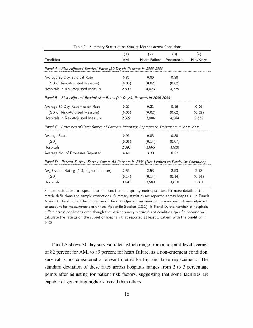
Table 2 presents basic summary statistics on the quality metrics. It shows clinicallyand economically meaningful dispersion across hospitals in all of the measures.
10 See http://goo.gl/FJ0Nvy and http://goo.gl/zeHg2J for this data.11See http://kff.org/medicare/state-indicator/enrollees-as-a-of-total-medicare-population/12The Dartmouth Atlas of Healthcare divides the United States into HRRs, which are determined
at the ZIP code level through an algorithm that reflects commuting patterns to major referral hospi-tals. HRRs, which are akin to empirically defined markets for healthcare, may cross state and countyborders. A complete list of HRRs can be found at http://www.dartmouthatlas.org/.
15
(1) (2) (3) (4)
Condition AMI Heart Failure Pneumonia Hip/Knee
Panel A - Risk-Adjusted Survival Rates (30 Days): Patients in 2006-2008
Average 30-Day Survival Rate 0.82 0.89 0.88
(SD of Risk-Adjusted Measure) (0.03) (0.02) (0.02)
Hospitals in Risk-Adjusted Measure 2,890 4,023 4,325
Panel B - Risk-Adjusted Readmission Rates (30 Days): Patients in 2006-2008
Average 30-Day Readmission Rate 0.21 0.21 0.16 0.06
(SD of Risk-Adjusted Measure) (0.03) (0.02) (0.02) (0.02)
Hospitals in Risk-Adjusted Measure 2,322 3,904 4,264 2,632
Panel C - Processes of Care: Shares of Patients Receiving Appropriate Treatments in 2006-2008
Average Score 0.93 0.83 0.88
(SD) (0.05) (0.14) (0.07)
Hospitals 2,398 3,666 3,920
Average No. of Processes Reported 4.40 3.30 6.22
Panel D - Patient Survey: Survey Covers All Patients in 2008 (Not Limited to Particular Condition)
Avg Overall Rating (1-3, higher is better) 2.53 2.53 2.53 2.53
(SD) (0.14) (0.14) (0.14) (0.14)
Hospitals 3,498 3,598 3,610 3,061
Table 2 - Summary Statistics on Quality Metrics across Conditions
Sample restrictions are specific to the condition and quality metric; see text for more details of the
metric definitions and sample restrictions. Summary statistics are reported across hospitals. In Panels
A and B, the standard deviations are of the risk-adjusted measures and are empirical-Bayes-adjusted
to account for measurement error (see Appendix Section C.3.1). In Panel D, the number of hospitals
differs across conditions even though the patient survey metric is not condition-specific because we
calculate the ratings on the subset of hospitals that reported at least 1 patient with the condition in
2008.
Panel A shows 30 day survival rates, which range from a hospital-level averageof 82 percent for AMI to 89 percent for heart failure; as a non-emergent condition,survival is not considered a relevant metric for hip and knee replacement. Thestandard deviation of these rates across hospitals ranges from 2 to 3 percentagepoints after adjusting for patient risk factors, suggesting that some facilities arecapable of generating higher survival than others.
16
Panel B shows that the average hospital-level readmission rate ranges from 6percent for hip and knee replacement to about 21 percent for AMI and heart failure.Like survival, the cross-facility standard deviations are 2 to 3 percentage pointsafter adjustment for patient risk factors.
Panel C reports on the process of care measure. In our allocation results, wecombine the condition-specific individual process of care scores into a single com-posite, standardized (i.e. mean 0 and standard deviation 1), condition-specific score.To give a sense of the metric, we present here for each condition a score that is gen-erated by taking each hospital’s average utilization of the condition’s processes,then averaging the result across hospitals. The reported score of 0.93 for AMImeans that for the average hospital, the average utilization rate across the 6 AMItreatments is 93 percent. Compliance with the processes is lower for heart fail-ure (83 percent) and pneumonia (88 percent). The dispersion in compliance acrosshospitals is larger than in risk-adjusted survival and readmission – it ranges from 5percentage points for AMI to 14 percentage points for heart failure.
The patient survey is reported in Panel D. In order to capture the full breadth ofquestions included in the survey in our allocation analyses, we mimic our approachfor the process of care metric and use a standardized (i.e. mean 0, standard deviation1) composite of all the survey questions. To give a flavor for the measures, PanelD reports the results of one of the questions: a patient-reported overall rating of thehospital. The table reports the average score across hospitals when low, medium,and high are valued at 1, 2, and 3 respectively. The average patient at the averagehospital gives between a medium and a high rating, and this is true even for thehospital two standard deviations below the average.
We examined the correlation of quality measures across hospitals and condi-tions. For a given hospital quality measure, hospital quality is strongly positivelycorrelated across conditions (see Appendix Table A4); for example, the within-hospital correlation of risk-adjusted readmission between the four conditions rangesfrom 0.44 to 0.94.
Table 3 examines the correlation of hospital quality measures within each con-dition (though as stated, the patient survey covers all patients). Higher values ofall these quality measures are desirable, except for risk-adjusted readmission. Most
17

of the correlations are of the expected sign: risk-adjusted survival and process ofcare are positively correlated, and risk adjusted readmission and process of care arenegatively correlated.13 However the correlations are substantially below 1, sug-gesting that these measures may be capturing different dimensions of the hospitalexperience.14
(1) (2) (3) (4) (5) (6) (7) (8)
Metric
Risk-Adj
Survival
Risk-Adj
Readm
Process
of Care Z
Patient
Survey Z
Risk-Adj
Survival
Risk-Adj
Readm
Process
of Care Z
Patient
Survey Z
Risk-Adjusted Survival 1.00 1.00
[2,890] [4,023]
Risk-Adjusted Readmission 0.03 1.00 0.35 1.00
[2,322] [2,322] [3,904] [3,904]
Process of Care Z-Score 0.24 -0.25 1.00 0.17 -0.15 1.00
[2,346] [2,214] [2,398] [3,607] [3,578] [3,666]
Patient Survey Z-Score -0.06 -0.26 0.18 1.00 -0.18 -0.36 0.01 1.00
[2,799] [2,293] [2,370] [3,498] [3,447] [3,398] [3,392] [3,598]
Metric
Risk-Adj
Survival
Risk-Adj
Readm
Process
of Care Z
Patient
Survey Z
Risk-Adj
Survival
Risk-Adj
Readm
Process
of Care Z
Patient
Survey Z
Risk-Adjusted Survival 1.00
[4,325]
Risk-Adjusted Readmission 0.08 1.00 1.00
[4,264] [4,264] [2,632]
Process of Care Z-Score 0.08 -0.18 1.00
[3,871] [3,847] [3,920]
Patient Survey Z-Score -0.03 -0.36 0.18 1.00 -0.23 1.00
[3,527] [3,503] [3,512] [3,610] [2,542] [3,061]
AMI HF
Table 3 - Correlation of Quality Metrics within Condition
Hospitals used to calculate correlation in brackets. All quality metrics are condition-specific except the patient
survey, which is only available as an all-patient average. Correlations involving risk-adjusted survival and
readmission are adjusted to account for measurement error (see Appendix Section C.3.2).
Pneumonia Hip/Knee Replacement
13Risk-adjusted survival and risk-adjusted readmission are positively correlated; this ostensiblysurprising pattern has been previously documented (see e.g. Gorodeski, Starling and Blackstone,2010) and at least partly reflects the fact that mortality and readmission are competing risks, sincepatients who die cannot be readmitted.
14Hospitals are multi-product firms that treat many different conditions. Understanding why per-formance correlates across outputs is beyond the scope of this study, but is a potentially fruitfulavenue for future research.
18

Patient satisfaction does not have a systematic correlation with our other qualitymeasures. As has been found previously in the literature (see e.g. Jha et al., 2008and Boulding et al., 2011), it is positively correlated with hospital performance asmeasured by readmission and process of care. However, we find that it is negativelycorrelated with risk-adjusted survival rates.15 These ambiguous findings for patientsatisfaction are not new to the quality measurement literature, and align with con-cerns of physicians who question the value of patient satisfaction as an informativemeasure of hospital quality (Manary et al., 2013).
IV Allocation Results
IV.A Static and Dynamic Allocation
Table 4 presents our central results. The left-hand panel shows static allocationresults based on the estimation of equation (1). These results relate the hospital’slog number of patients for a given condition in 2008, ln(Nh), to a given qualitymeasure for that hospital in 2008, qh. Because we include market (HRR) fixedeffects, this estimate is within market, relating a hospital’s market share of patientswith a given condition to its quality relative to other hospitals in its market. Eachpanel shows results from a separate regression using the reported quality measure.
15In Appendix Table A5 we also find that patient satisfaction tends to be negatively correlated withthe Bloom et al. (2012) measure of hospital management quality for the several hundred hospitalsfor which this measure is available, while both risk-adjusted survival and process of care scoresare positively correlated with hospital management scores; there is no clear pattern with respect torisk-adjusted readmission. We are extremely grateful to Nick Bloom for providing us with thesemeasures.
19

(1) (2) (3) (4) (5) (6) (7) (8)
Measure \ Condition AMI HF Pneu Hip/Knee AMI HF Pneu Hip/Knee
Coef on Survival Rate 17.496 15.360 5.140 1.533 0.774 1.220
(0.995) (1.320) (0.777) (0.379) (0.501) (0.354)
Hospitals 2,890 4,023 4,325 2,890 4,023 4,325
Coef on Readmission Rate -9.162 -10.346 0.499 -21.037 -1.428 -2.300 -1.138 -1.112
(1.621) (1.782) (1.575) (2.027) (0.611) (0.651) (0.679) (0.836)
Hospitals 2,322 3,904 4,264 2,632 2,322 3,904 4,264 2,632
Coef on Process Z-Score 0.319 0.332 0.211 0.048 0.043 0.026
(0.026) (0.016) (0.015) (0.010) (0.009) (0.009)
Hospitals 2,398 3,666 3,920 2,398 3,666 3,920
Coef on Survey Z-Score -0.321 -0.252 -0.210 0.057 -0.065 -0.003 0.007 0.037
(0.052) (0.038) (0.030) (0.051) (0.015) (0.011) (0.011) (0.022)
Hospitals 3,498 3,598 3,610 3,061 3,498 3,598 3,610 3,061
Table 4 - Allocation across Conditions
The static allocation results are estimated using equation (1), a hospital-level regression of log-patients in 2008 on
market fixed effects and the quality measure named in the row. The dynamic allocation results are estimated using
equation (2), which is an identical regression except for the dependent variable, which is now growth in patients
from 2008 to 2010. Growth is defined as in equation (3). Standard errors are bootstrapped with 300 replications
and are clustered at the market level. Risk-adjusted survival and readmission are reported in percentage points (e.g.
a value of 0.1 is 10 percentage points); process of care and patient survey metrics are reported in standard deviation
units (e.g. a value of 1 is 1 standard deviation).
Static Allocation Dynamic Allocation
Risk-Adjusted Survival
Risk-Adjusted Readmission
Process of Care Z-Score
Patient Survey Z-Score
We find a statistically significant and positive relationship between hospitalquality and market share for three of the four quality metrics (risk-adjusted sur-vival, risk-adjusted readmission, and process of care). This suggests that, within amarket, more market share (patients) tends to be allocated to higher quality hospi-tals at a point in time. For AMI patients (column 1), our estimates indicate that a 1percentage point increase in a hospital’s risk-adjusted AMI survival rate is associ-ated with a 17 percent higher market share (or equivalently, due to the presence ofmarket fixed effects, 17 percent more patients), a 1 percentage point reduction in thehospital’s readmission rate is associated with 9 percent more patients, and a 1 stan-dard deviation increase in the use of consensus AMI treatments (processes of care)
20

is associated with 32 percent more patients; all of these results are statistically sig-nificant. For heart failure patients (column 2) results are similar in magnitude andstatistical significance. For pneumonia patients (column 3) the results are smaller inmagnitude but still statistically significant for risk-adjusted survival and process ofcare; they are wrong-signed but insignificant for risk-adjusted readmission. For hipand knee replacement (column 4) we only observe the risk-adjusted readmissionmeasure, which is statistically significant with the expected sign.
The right-hand panel shows dynamic allocation results based on the estimationof equation (2). These estimates examine the within-market relationship between ahospital’s quality qh and its subsequent two-year growth ∆h, as defined in equation(3). Again, each panel shows results from a separate regression using the reportedquality measure. The results once more tend to show a statistically significant pos-itive relationship between measures of hospital quality and market share, with theexception of the patient satisfaction survey. For example, for AMI the results in-dicate that a 1 percentage point increase in the hospitals’s risk-adjusted survivalrate is associated with 1.5 percentage points higher growth in AMI patients relativeto other hospitals in the same market. A hospital with a 1 percentage point lowerrisk-adjusted AMI readmission rate would tend to grow its AMI patient load 1.5percentage points faster than other hospitals in the market, and a 1 standard devi-ation increase in utilization of AMI processes of care is associated with 4.8 per-centage points higher growth. All of these results are statistically significant. Theresults are similar for the other three conditions – with higher risk-adjusted sur-vival, lower readmission, and better process of care scores associated with greatertwo-year growth – and they are mostly (but not always) statistically significant.
The patient survey score is an exception to our general finding that higher qual-ity hospitals tend to be larger (in the static allocation results) and grow faster (inthe dynamic allocation results) than their peers. As previously discussed, hospitals’scores on the patient satisfaction survey are negatively correlated with some of ourother quality metrics, and there is debate over the survey’s value as a measure ofhospital quality. These facts may explain our findings. Alternatively, the fact thatmarket share appears correlated with the health and process of care measures ratherthan patient satisfaction could reflect which factors drive the demand of patients or
21

their surrogates. For example, patients may not know or may not value features onthe survey such as how quiet rooms are at night. It is also possible that – as the onequality metric that is not condition-specific – the patient satisfaction measure hasless relevance for the condition-specific allocation decisions.
To probe a little further on the different quality metrics, we also analyzed alloca-tion putting the whole vector of quality metrics on the right-hand side of equations(1) and (2). Appendix Table A6 reports the results. Not surprisingly, given thatthese variables are highly correlated (see Table 3), the magnitude of the coefficientson the individual quality metrics often attenuate and, for many of the dynamic anal-yses, are no longer statistically significant.16 Overall, however, they suggest anassociation between market share and each individual quality measure, conditionalon the others, that is qualitatively similar to the unconditional correlations shown inTable 4.
We also considered the relationship between allocation for a given conditionand quality measures for multiple conditions included in the regression simultane-ously. Appendix Table A8 shows the results. Again, we find that multiple qualitymeasures tend to matter. While own-condition quality usually remains a significantpredictor of allocation, allocation generally loads onto several conditions’ qualitymeasures, and the AMI quality measure is often the most quantitatively important.These results likely reflect that within-hospital quality is highly correlated acrossconditions (see Table A4), and that our condition-specific quality measures are eachnoisy measures of underlying condition quality. The AMI measures may offer rel-atively more precise signals in comparison to the measures of the other conditions,or they may be more salient to consumers.
Robustness
We examined the robustness of our main allocation findings in Table 4 along a num-ber of dimensions. As previously discussed, we show our static allocation results
16Part of the weakening of the results is also due to the fact that we limit the multivariate analysisin Appendix Table A6 to the subset of hospitals that report all four quality measures. AppendixTable A7 shows that when we run the allocation results separately for each quality measure as inTable 4 but limited to this subset of hospitals for which all four quality measures are available, thecoefficients are somewhat attenuated relative to our baseline results.
22

are robust to alternative ways of handling the truncation on sample size (see foot-note 6 and Appendix Table A1). We also show that our core allocation findings forsurvival and readmission remain without the empirical Bayes adjustment, althoughnaturally the magnitude is attenuated (see footnote 7 and Appendix Table A2). Fur-thermore, we find that our static allocation analysis is not sensitive to an alternativespecification, Poisson regression (see Appendix Table A9).
Finally, we explored the sensitivity of our findings to how we handle risk adjust-ment. A potential concern with both the survival and readmission quality measuresis that they may be capturing heterogeneity in patient health across hospitals; thisconcern is muted for the process of care measures, which exclude patients whowere inappropriate for each standard of care. Fortunately, there exist rich data onthe relevant health characteristics of the patients (called risk-adjusters) which weuse in creating our survival and readmission metrics. Of course, such risk adjust-ment is only as good as the observable characteristics on which it is based. Riskadjustment for AMI based on our observables has recently been cross-validated byresearch exploiting ambulance catchment areas as a source of exogenous variationin the allocation of patients to hospitals (Doyle, Graves and Gruber, 2014). In Ap-pendix Table A10 we show that the results are only slightly affected if we insteaduse coarser risk adjustment (age/race/sex only) or no risk adjustment at all. Theseresults help mitigate concerns that additional risk adjustment would attenuate oreliminate our findings. Moreover, we showed in previous work that additional riskadjustment with extremely rich data (available for a subset of AMI patients) haslittle effect on allocation results (Chandra et al., 2013).
IV.B Benchmarking the magnitude of reallocation
IV.B.1 Quality vs. distance
As one way of benchmarking the magnitude of our allocation results, we comparedthe reallocation of market share associated with higher quality to the reallocationassociated with shorter distance between patient and hospital. Distance-to-hospitalis a classic hospital attribute that has been extensively analyzed as a measure ofhospital “price”, with the general finding that individuals consider greater distance
23

to the hospital as a disamenity (see e.g. Luft et al., 1990; Town and Vistnes, 2001;Gaynor and Vogt, 2003; Tay, 2003; Romley and Goldman, 2011).
To compare allocation on quality to that on distance, we adapt our static al-location analysis in the spirit of the existing distance-to-hospital choice literature.Specifically, we specify the utility function of consumer p for hospital h as:
(4) Uph = ρ1 ·distanceph +ρ2 ·distance2ph +θ ·qh +ϕph.
Uph is the utility of a potential choice, distanceph is the distance from the patientto the hospital (entering as a quadratic; operationally we measure the distance fromthe patient’s ZIP code of residence to the hospital’s ZIP code), and qh is the hos-pital’s quality metric. There is also a component of utility that is idiosyncratic tothe patient-hospital pair ϕph. We assume that ϕph is distributed type 1 extremevalue, which means the problem can be readily estimated as a conditional logit, asis standard in the hospital choice literature (e.g. Dranove and Satterthwaite, 2000).
When consumers maximize this utility function, the realized choice probabili-ties are:
(5) Pr(Cp = h) =exp(
ρ1 ·distanceph +ρ2 ·distance2ph +θ ·qh
)∑h′∈HM(p)
exp(
ρ1 ·distanceph′+ρ2 ·distance2ph′+θ ·qh′
) ,where Cp indicates the hospital that the patient chose for treatment and HM(p) isthe patient’s choice set of hospitals; we define the choice set as all hospitals inthe patient’s hospital market M (p) that treat at least 1 patient with that conditionin 2008 and for which we observe the relevant quality metric. Because of ourdefinition of the patient’s choice set, our analysis – unlike the allocation analysis inTable 4 – excludes any patient who left her market of residence for treatment. Asshown in Appendix Table A11, this restriction excludes 10 to 16 percent of patientsdepending on the condition, but does not affect the basic static allocation results.
Table 5 presents the results from the conditional logit choice model. Acrossthe columns are different health conditions. The panels report the marginal rates of
24

substitution (MRS) between a given quality metric and distance; each panel showsthe results from a separate regression using the reported quality measure (AppendixTable A12 presents the raw logit coefficients). The reported marginal rate of substi-tution of quality for distance, evaluated at the average distance traveled by patientsfor that condition, is derived from the conditional logit estimates as:
(6) MRS =∂Uph/∂qh
∂Uph/∂distanceph=
θ
ρ1 +2 ·ρ2 ·distance.
When the MRS is negative, it implies that the quality measure is a good, i.e. thatpatients are willing to travel farther to gain access to more quality. When it ispositive, it implies that the quality metric is a bad.
25

(1) (2) (3) (4)
Condition AMI HF Pneumonia Hip/Knee
Mean Miles to Chosen Hospital 12.48 8.27 7.49 13.16
SD Miles to Chosen Hospital 20.06 13.25 11.92 18.85
MRS(1 pp risk-adjusted survival, miles) -1.793 -1.029 -0.378
(0.158) (0.129) (0.057)
Patients 165,005 275,671 317,904
MRS(1 pp risk-adjusted readmission, miles) 1.138 1.040 0.451 2.385
(0.173) (0.122) (0.109) (0.268)
Patients 158,086 274,667 317,374 222,673
MRS(1 SD process of care, miles) -4.418 -2.238 -1.325
(0.383) (0.221) (0.110)
Patients 158,032 270,773 309,623
MRS(1 SD patient survey, miles) 0.324 -0.093 0.036 -1.604
(0.388) (0.205) (0.151) (0.382)
Patients 167,429 266,915 298,185 224,451
Table 5 - Choice Model of Patient Allocation across Conditions
This table reports the marginal rates of substitution (MRSs) of quality for distance derived from the conditional
logit model (see equation 6). For the survival and readmission rates, the MRS given by equation (6) is divided by
100 to put it into percentage point terms. Only one quality measure is used at a time in each logit model.
Standard errors are analytic and clustered at the market level.
The sample is all patients with the condition in 2008 who stayed in their market of residence for treatment. The
choice set for a patient is all hospitals in his market with the quality measure available that treated at least one
patient in 2008. The mean and SD miles statistics are taken from the patients in the column’s risk-adjusted
survival sample (risk-adjusted readmission for hip/knee replacement). All MRSs in a column are evaluated at this
mean.
Risk-Adjusted Survival
Risk-Adjusted Readmission
Process of Care Z-Score
Patient Survey Z-Score
Qualitatively, our results are what would be expected given the existing liter-ature and the results from our static allocation analysis: hospital choices are con-sistent with a willingness to travel longer distances in order to receive treatment atfacilities with better health outcomes and processes, but not higher patient surveyscores. Quantitatively, the results indicate that the average AMI patient is willing totravel 1.8 more miles (about one-tenth of the standard deviation of distance traveledfor AMI) to gain access to a hospital with 1 percentage point greater risk-adjustedsurvival, 1.1 miles for 1 percentage point lower risk-adjusted readmission, and 4.4
26

miles for 1 standard deviation unit greater use of processes of care.17
These results are broadly similar to other estimates of “willingness to travel”to a different hospital. Perhaps most directly comparable to our estimates is Tay(2003)’s analysis of hospital choice for Medicare patients with AMI in 3 states in1994. She finds that distance, hospital mortality rates, and hospital complicationrates are all disamenities in patients’ hospital choices. Her results imply, for ex-ample, that younger white male patients are willing to travel 8.0 miles to accessa hospital with a 1 percentage point lower mortality rate and 1.7 miles to accessa 1 percentage point lower complication rate. In addition, Romley and Goldman(2011) look at hospital demand for Medicare patients with pneumonia within LosAngeles over 2000-2004 and estimate a a willingness to travel ranging from 2.4 to3.9 miles to move from the hospital at the 25th to 75th percentile of the distributionof hospitals’ revealed utility.
IV.B.2 Contribution to survival gains
Another way to benchmark the allocation results is to explore their contribution tothe secular improvements in survival gains for individuals hospitalized with theseconditions. To do so, we expand our analysis period to track risk-adjusted survivalfrom 1996 through 2008. The conventional wisdom is that the driving forces behindsurvival gains over this time period are a combination of ‘high-tech’ and ‘low-tech’adoption decisions by hospitals (Cutler, 2005; Chandra and Skinner, 2012). Butaverage survival gains can also come from reallocation of patients toward hospi-tals that achieve better outcomes. We investigate the extent to which the observedgrowth in average survival can be attributed to reallocation to higher quality hospi-tals as opposed to quality improvements within hospitals.
We use the approach of Foster, Haltiwanger and Krizan (2001) and Foster, Halti-wanger and Syverson (2008), which is itself a modification of the decompositionfirst derived in Baily et al. (1992). Specifically, we decompose the change in theaverage risk-adjusted 30-day survival in a market as follows:
17The results are qualitatively similar for the other conditions, though magnitudes are oftensmaller – indicating that for these conditions, patients are somewhat less willing to travel additionaldistance for a given increment in quality.
27

∆qt = ∑h∈Ct
θh,t−1∆qh,t︸ ︷︷ ︸within
+ ∑h∈Ct
(qh,t−1− qt−1
)∆θh,t︸ ︷︷ ︸
between
+ ∑h∈Ct
∆qh,t∆θh,t︸ ︷︷ ︸cross
(7)
+ ∑h∈Mt
θh,t(qh,t− qt−1
)︸ ︷︷ ︸
entry
− ∑h∈Xt
θh,t−1(qh,t−1− qt−1
)︸ ︷︷ ︸
exit
where qt is the market-share-weighted average 30-day survival across hospitals inthe market in year t, and ∆ is the difference operator; thus the left-hand side is thechange in weighted average patient survival in the market between two periods. Onthe right hand side, qh,t is the risk-adjusted survival rate for hospital h in year t andθh,t is its market share, i.e. the share of patients in the market with the conditionwho were treated at that hospital. Ct is the set of hospitals that were open in botht−1 and t; Mt is the set of hospitals that entered the market in t, and Xt is the set ofhospitals that exited the market between t−1 and t.18
The decomposition in equation (7) divides average survival growth into fiveterms. The first term, “within”, reflects changes in average survival in the mar-ket due to survival improvements among continuing hospitals holding their marketshares constant. These are the survival gains that would have been attained in ab-sence of any reallocation. The remaining terms reflect reallocation effects on aver-age survival in the market. The second term, “between”, shows how much of therise is due to patients reallocating to hospitals that were already of high quality. Themiddle term, “cross”, captures the covariance between gains in survival and gainsin market share; it indicates whether hospitals that raised quality also grew theirpatient loads. The final two terms are, respectively, gains in survival due to enteringhospitals having better performance than the previous average and the gains due tolower than average performance hospitals exiting. Any of these five terms could ofcourse be negative if changes in survival, shares, or the composition of hospitalswere such as to detract from average survival rates in the market.
18Because measurement error in risk-adjusted survival does not cause bias in any of the terms ofthis decomposition, we do not empirical-Bayes-adjust the survival measure when computing thesemetrics.
28

We look at the long difference between t = 2008 (our baseline period) and t−1 = 1996. To do this, we replicated our sample selection and risk-adjusted survivalmeasure in the 1996 data.19 Thus ∆qt represents the change in 30-day survivalbetween 2008 and 1996 for the market.20 After conducting the decomposition foreach market, we average each component over all markets weighting by the initialnumber of patients in the market in 1996. The resulting averages reflect the extentto which each of the five components accounted for survival gains over the 12-yearperiod.
Table 6 displays the results. The first row shows the substantial secular improve-ment in survival gains for individuals hospitalized with these conditions. Average30-day survival increased across all HRRs by 3.9 percentage points for AMI, 0.9percentage points for heart failure, and 3.2 percentage points for pneumonia. Theacademic literature has focused on progress in AMI-survival – presumably becauseit is most dramatic – and attributed the improvements to technological progress. Theliterature has credited medically intensive interventions such as stents and reperfu-sion therapy and low-cost medical interventions such as aspirin and β blockers (Fib-rinolytic Therapy Trialists’ Collaborative Group, 1994; Keeley and Hillis, 2007;Chandra and Skinner, 2012).
19Specifically, just as in our baseline analysis for 2008 we measure risk-adjusted survival using2006-2008 data and market share with 2008 patient counts, so for our 1996 analysis we measurerisk-adjusted survival using 1994-1996 data and market share with 1996 patient counts. We use thesame approach to define the sample and implement the risk-adjustment for the 1996 analysis as forthe 2008 analysis.
20We centered the risk-adjusted survival measure qh,t in each market so that its market-shareweighted average qt equalled that of the raw, market-year average survival measure.
29

(1) (2) (3) (4) (5) (6)
Condition AMI HF Pneu AMI HF Pneu
Total Change in Wtd Survival 0.0389 0.0092 0.0316 1.00 1.00 1.00
Within 0.0298 0.0076 0.0297 0.77 0.82 0.94
Between 0.0000 -0.0004 -0.0004 0.00 -0.05 -0.01
Cross 0.0062 0.0015 0.0015 0.16 0.16 0.05
Entry 0.0021 0.0006 0.0010 0.05 0.07 0.03
Exit -0.0007 0.0000 0.0002 -0.02 0.01 0.01
Table 6 - Decomposition of Gains in Survival Over Time
Contributions in Pctage Points Contributions as Share of Total
This table decomposes the gains in risk-adjusted survival for the emergent conditions over our
full sample window (between 1996 and 2008) using the decomposition shown in equation (7).
Columns 1-3 show the contribution of each component to gains in survival in percentage points
(e.g. a value of 0.1 is 10 percentage points). Columns 4-6 show the share of total gains that can
be attributed to each component. The exit component enters negatively, so a negative value
indicates that exit accounts for a gain in survival.
The decomposition is performed for each market, then averaged together weighted by the
market's size in 1996. Risk-adjusted survival is calculated from a regression of survival on
hospital fixed effects and patient risk-adjusters. A separate regression is run for each of the year
groups 1994-1996 (yielding the 1996 survival rates) and 2006-2008 (yielding the 2008 survival
rates).
Consistent with this conventional wisdom, we find that within-hospital upgrad-ing in quality accounts for the bulk of the AMI improvements, explaining 77 per-cent of gains in risk-adjusted AMI survival over our 12 year period. However, wealso find a quantitatively important role for reallocation; 23 percent of the secularimprovement in AMI survival can be explained by reallocation of patient flows to-ward higher quality hospitals. The cross term explains the bulk of the reallocationgains, contributing 0.6 percentage points (16 percent of the total gains). Entry ofhigh-performance hospitals can explain about 0.2 percentage points (5 percent) ofsurvival gains, and exit of low-performance hospitals can explain about 0.1 percent-age points (about 2 percent) of survival gains.21
21Due to our sample constructions, “exit” and “entry” need not be literal hospital entry and exit.They also reflect a reduction in condition-specific sample size below the inclusion cutoff (specifi-cally, at least 25 patients in the three year period used to estimate risk-adjusted survival and at least1 patient in the final year; see Section III.B).
30

To put the role of reallocation in AMI survival gains in perspective, it is instruc-tive to note that the nearly 1 percentage point improvement in AMI survival overthe 1996-2008 period that we attribute to reallocation is about half of the magni-tude of the survival gains attributed to each of two major breakthroughs in AMItreatment: reperfusion and primary angioplasty. Reperfusion (including e.g. fib-rinolytics) started being widely used in the early 1990s and has been estimated toraise 30-day survival by 2 percentage points (Fibrinolytic Therapy Trialists’ Col-laborative Group, 1994). Primary angioplasty diffused over the 1990s and has beenestimated to increase 30-day AMI survival by 2 percentage points over reperfusiontherapy (Stone, 2008; Keeley, Boura and Grines, 2003).
For heart failure and pneumonia – where the secular improvements in survivalare noticeably smaller – we find a somewhat smaller contribution of reallocation.Table 6 indicates that reallocation can explain about 18 percent of the 0.9 percentagepoint secular improvement in heart failure survival and about 6 percent of the 3.2percentage point improvement for pneumonia.
Using our long survival panel to explore whether the relationship between mar-ket allocation and hospital performance has evolved over time, we find that thealignment of market allocation with hospital performance appears to have increasedsince 1996.22 This could be because information about hospital quality and hospi-tal outcomes has become more available to patients and their surrogates. The studysample corresponds to a period in which tools like CMS Hospital Compare madeit much easier for patients to ascertain the quality of a hospital, and research onthe impact of report cards has found some evidence of consumers responding to in-formation therein (Dranove et al., 2003; Dranove and Sfekas, 2008). Alternatively,patients’ willingness or ability to switch among hospitals may have risen for otherreasons. For example, the consolidation of either insurers or provider groups mayhave induced consumers to reallocate to higher quality providers. Clearly, these
22Appendix Table A13 shows these results. We report the static and dynamic allocation analysisof equations (1) and (2) for five separate periods: 1996, 1999, 2002, 2005, and 2008. We find that al-location tends to become more directed toward high-survival hospitals over the sample. AMI has thecleanest such pattern; the magnitudes of both static and dynamic allocation increase monotonicallyover the sample. Heart failure and pneumonia are noisier, especially for the dynamic allocation, buttheir overall trends are in the same direction.
31

channels are speculative; we do not have the necessary data to pin down the mecha-nism in this study, but we see this as a natural and interesting area for future work.
IV.C Private vs. Social Preferences
Thus far we have examined the correlation of market share with a variety of “qual-ity” and “output” metrics, with no attention to hospital inputs or costs. Uniquely inthe health care sector relative to the rest of the economy, consumers absorb little tonone of the costs of their hospital choice. The Medicare patients we analyze all haveinsurance with limited cost-sharing, much of which in turn is covered by supple-mental (public or private) coverage (MEDPAC, 2012). As a result, an output-basedquality metric is likely the relevant one from the perspective of consumer demand;we would not expect patients or their surrogates (family members, physicians, etc.)to substitute away from high cost hospitals.
A benevolent social planner, on the other hand, would want to allocate towardhospitals with high quality (output) conditional on inputs. How the social plannerwould trade off higher output at the cost of higher inputs would, of course, dependon the the social welfare function. We therefore analyze how allocation correlateswith productivity, which we define as the hospital’s ability to generate survival con-ditional on the inputs it uses in the treatment process. Because the social planneris concerned about conditional survival while the patient values unconditional sur-vival, there may be a wedge between the socially and privately optimal hospitalchoice.
To analyze whether the market re-allocates toward some measure of input-adjusted outcomes, we define a patient-level health production function of the fol-lowing form:
(8) Y sp = Ah
(∏
kRλk
pk
)X µ
p Ξp.
where the leading term, Ah, measures the exponential of total factor productivity(TFP) of hospital h; Y s
p is the output generated by the hospital in treating patient
32

p; and Xp is a measure of hospital inputs used to treat the patient. All productionfunctions relate outputs to inputs; our particular function uses 30-day survival as ameasure of output (in fact, Y s
p is technically the exponential of this indicator) and asingle index of resources spent on the patient as inputs.23 The parameter µ is theelasticity of 30-day survival with respect to risk-adjusted inputs. Because patientsare inherently heterogeneous, survival may also depend on characteristics of thepatient, which could potentially also be correlated with input choices. In addition,the marginal effect of inputs on survival may vary with patient characteristics. Tocapture both of these effects, we follow the literature and adjust inputs for a vectorof observable patient-level risk factors, Rpk, where k indexes the factors. The riskfactors are the same as those used in the calculation of risk-adjusted survival de-scribed in Appendix B. Finally, the expression Ξp is a patient-level error term thataccounts for random variations in health outcomes.
The hospital production function model in equation (8) allows variation acrosshospitals in the marginal health product of inputs but constrains hospitals to have thesame elasticity of output with respect to input (i.e., µ is common across hospitals).Our empirical specification therefore allows the "marginal return to inputs" curveto vary across hospitals, as suggested by Chandra and Staiger (2007) and Garberand Skinner (2008).
Taking logs and using lowercase letters to represent the logarithm of uppercaseletters yields our estimating equation for the hospital production function:
(9) ysp = ah +∑
kλkrpk +µxp +ξp
This equation is identical to what we use to estimate risk-adjusted survival (seeAppendix B for more details) with one key difference: it controls for logged hospitalinputs xp. Hospital productivity ah is risk- and resources-adjusted survival – orequivalently, hospital output conditional on inputs (which include patient healthinputs, i.e. the risk-adjusters we used previously to construct risk-adjusted survival,
23This sort of single-input production function is unusual but convenient; one could reasonablyinterpret the single input as an index of the use of multiple inputs that go into producing health.
33

as well as resource inputs).A key challenge in calculating productivity is constructing an appropriate mea-
sure of hospital inputs. These inputs are the resources utilized in the treatment ofthe patient – labor inputs like physicians and nurses and capital inputs like the op-erating theater and diagnostic scanners. Measuring inputs is challenging in mostindustries, and healthcare is no exception. In practice, we consider two imperfectmeasures of these inputs.
Our first input measure is federal expenditures, i.e. total Medicare dollar pay-ments to hospitals for inpatient services used in the treatment of the patient duringthe first 30 days following the admission. Medicare pays hospitals for each patientstay; its reimbursement for a hospital stay is based on the diagnosis causing theadmission, whether the patient has other complicating medical conditions, the geo-graphic location of the hospital, the type of hospital (e.g. whether it is an academicmedical center) and, to some extent, what is done to the patient in the hospital (Med-PAC, 2011). For example, within a given hospital, Medicare reimbursement for anAMI admission will vary depending on the presence of a complicating conditionlike heart failure or stroke and whether the patient receives various intensive treat-ments such as a bypass operation; Medicare spending over the 30 days followingthe index admission will also depend on whether the patient has multiple hospitalstays, as each stay triggers an additional Medicare payment.
Using federal expenditures as our input measure allows us to construct a mea-sure of output (survival) per dollar of federal expenditures. Given the social costof raising public funds, this is a natural and useful productivity metric. However, ithas the disadvantage that it captures variation in inputs coming both from hospital-specific prices and CMS’s estimates of the real resources used by the hospital fortreatment. Our second input measure addresses this concern by purging the fed-eral spending measure of pricing variation to create a “resource” measure of inputs.Specifically, we define hospital inputs for a patient as the sum of diagnostic-relatedgroup (or DRG) weights during the first 30 days following a heart attack. TheseDRG weights reflect CMS’s assessment of the resources necessary to treat a patientas a function of the patient’s medical conditions and procedures received. This ap-proach is standard in the literature as a way of purging measures of care utilization
34

of administrative price variation (see e.g. Skinner and Staiger, 2015; Gottlieb et al.,2010). Nonetheless, it is a highly imperfect measure of inputs, as it does not reflectactual inputs used but rather CMS-defined expected inputs based on the treatmentapproach chosen.
We limit our analysis to AMIs. We do this because for the other conditions,the vast majority of patients fall into just one or two DRGs. As a result, for theseconditions, there is little useful variation in the input measures for us to exploit.
We estimate the hospital production function in equation (9) for each input mea-sure using the same sample and risk-adjusters as we used to estimate risk-adjustedsurvival (described in Appendix B).24 Having estimated the production functionmodels for each input measure, we then extract the hospital fixed effects to createour estimates of productivity.
Table 7 examines static and dynamic allocation of AMI patients as a functionof these hospital productivity measures (i.e. the ah estimated in equation 9).25
Columns 1 and 2 consider static allocation with respect to productivity by the “fed-eral dollars” and “real resources” metrics, respectively. Both results imply that ahospital that can generate 1 percentage point greater survival holding inputs con-stant (i.e. has 1 percentage point greater TFP) is expected to be about 18 percentlarger than other hospitals in its market. Columns 5 and 6 repeat this analysis look-ing at dynamic allocation; for both measures, we find that having 1 percentagepoint greater TFP is associated with 1.5 percentage points higher growth in patientsbetween 2008 and 2010, compared to other hospitals in the market.
24Estimating this model with the federal dollars inputs measure yields µ=0.035 (standard error= 0.001). In other words, a 10 percent higher payment to the hospital for treating an AMI patientis associated with a 0.35 percentage point increase (0.4 percent of the hospital average survival rateof 0.82) in the probability of post-AMI 30-day survival. Using the resource-based input measureto estimate the hospital production function yields µ=0.042 (standard error = 0.001); increasingresources on a patent by 10 percent is associated with a 0.42 percentage point (0.5 percent) increasein the probability of post-AMI 30 day survival.
25We empirical-Bayes-adjust the hospital productivity objects when using them in the regressionsof Table 7 so that our coefficients are not biased due to measurement error. The empirical Bayesapproach is described in Appendix C and is identical to our approach for risk-adjusted survival andreadmission.
35

(1) (2) (3) (4) (5) (6) (7) (8)
Measure
Productivity (Fed $) 17.637 1.491
(1.118) (0.420)
Productivity (Resources) 17.540 1.471
(1.013) (0.386)
Risk-Adjusted ln(Fed $) 1.447 0.246
(0.169) (0.064)
Risk-Adjusted ln(Resources) 0.620 0.468
(0.406) (0.162)
Risk-Adjusted Survival 17.940 19.789 1.479 1.559
(1.192) (1.297) (0.446) (0.441)
Hospitals 2,890 2,890 2,890 2,890 2,890 2,890 2,890 2,890
Table 7 - Allocation of AMI with Respect to AMI Productivity and its Components
This table extends the analysis of Table 4 but is limited to static and dynamic allocation for AMI. It shows how
allocation is related to AMI productivity or its two components (risk-adjusted survival and risk-adjusted log-inputs).
Productivity is defined as risk- and inputs-adjusted survival; see Section 4.3 and equation (9). We consider two input
measures, "federal expenditures" and "resources", also defined in the text. Standard errors are bootstrapped with 300
replications and are clustered at the market level.
The standard deviation of productivity is 0.03 (Fed $ or Resources), of risk-adjusted log-inputs is 0.22 (Fed $) and 0.07
(Resources), and of risk-adjusted survival is 0.04 − this number differs from that of Table 2 because it comes from
estimating the joint distribution of survival and inputs, not survival alone.
Static Allocation for AMI Dynamic Allocation for AMI
These results show that market reallocation occurs in the direction of higherproductivity hospitals. However, as noted, if patients or their surrogates are makingthe allocation decision, they should not have reason to penalize hospitals which,conditional on output, are high input utilizers. In other words, they value healthoutcomes, not input-adjusted outcomes or “productivity”. The social planner, how-ever, would penalize hospitals that, conditional on health outcomes, had higherinputs (costs). We therefore examined the (conditional) correlation between alloca-tion and risk-adjusted survival and risk-adjusted inputs.26
The results – shown in the remaining columns of Table 7 – are consistent withthe social planner’s goal of rewarding hospitals with high performance after adjust-
26Risk-adjusted input use is defined as the hospital fixed effect from the regression of log-inputson the patient risk-adjusters and hospital fixed effects. Risk-adjusted survival is defined as it was pre-viously (see Appendix B). As with our productivity estimates, we use an empirical Bayes correctionto adjust our estimates of risk-adjusted survival and of risk-adjusted inputs for measurement error;our procedure, described in Appendix Section C.4, accounts for the correlation in measurement errorbetween these two objects.
36

ing for inputs. However, the market does not reallocate away from hospitals withhigher input use conditional on survival as the social planner would want.27 Put an-other way, higher productivity hospitals do treat more patients and grow faster, butthis is a result of the coincidence of high productivity with high output or quality(which our results indicate patients do respond to) rather than patients systemati-cally avoiding hospitals that use a lot of inputs to achieve high output.
This result illustrates the divergence between the goals of the social plannerand the consumer in a market where consumers face few costs. Indeed, it appearsthat, conditional on output, higher inputs are also associated with greater patientflow, although the magnitude of reallocation based on inputs is substantially smallerthan that based on output.28 It may be the case that consumers (correctly or not)view inputs conditional on outputs as a signal of unobserved quality, or that theyhave preferences for high intensity care regardless of its medical value, as has beenconjectured to have occurred in the past when hospitals competed on technologyin a “medical arms race” (e.g. Kessler and McClellan, 2000). With nearly fullinsurance for hospital treatment, there is no demand-side force in the market forAMI treatment to counteract these preferences and align the consumer’s preferenceswith those of the social planner. To push back against this consumer insensitivity, in2015 Medicare began penalizing hospitals with high costs by adding per-beneficiaryspending to the measures it uses to adjust payments in its Value-Based Purchasing
27Columns 3, 4, 7 and 8 show that the market reallocates both to hospitals with higher survival(conditional on inputs) and higher inputs (conditional on survival). The coefficient on productivitycan remain positive when used as a single index (columns 1, 2, 5, and 6) because the coefficientson risk-adjusted inputs are smaller than those on risk-adjusted survival and because risk-adjustedinputs are a smaller component of variation in productivity than risk-adjusted survival, since theyenter after being multiplied by µ � 1.
28For example, in the static allocation analysis, column 4 indicates that a 1 standard deviationincrease in outputs (i.e. risk-adjusted survival) is associated with a 69 percent rise in hospital size,while a 1 standard deviation increase in real resources-based inputs is associated with just a 5 percentrise in size.
In the static analysis, we find substantially larger reallocation toward inputs measured by federaldollars (column 3) than real resources (column 4), but this difference is an artifact of the CMSpayment approach; the Medicare payment formula explicitly pays academic medical centers andsafety net hospitals more than other hospitals for the same patient, and these facilities tend to belarge, which magnifies the correlation between federal dollars and size. The “real resources” inputmeasure accounts for this concern by using the same DRG weight (our measure of inputs) across allhospitals for each type of case.
37

Program (Kahn et al., 2015; QualityNet, 2015).
V Mechanism
The previous section showed, through multiple quantitative lenses, evidence of re-allocation to higher quality hospitals. A natural concern with these findings is thatthey purport to show the results of a reallocation process without giving evidence ofa mechanism by which such reallocation can occur. In this section we provide addi-tional evidence consistent with a demand-based mechanism and investigate leadingalternative explanations.
V.A Evidence of demand-based mechanism
We view the need to find additional signposts of demand-driven allocation as par-ticularly important given that intuition suggests that there may be little scope forpatient choice. In particular, for our three emergency conditions, AMI, heart fail-ure and pneumonia, about three-quarters of admissions come via the emergencydepartment. Relatedly, there is a long tradition in health economics – dating backat least to McClellan, McNeil and Newhouse (1994)’s analysis of hospital choiceby AMI patients – of using the distance from the patient’s residence to the nearesthospital as an instrument for which hospital the patient goes to. How, then, is itplausible that patients’ (or their surrogates’) demand is playing an allocative role insuch emergency situations?
As discussed in Section II and Appendix A, a key comparative static of a demand-based allocation mechanism is that as consumer’s ability or willingness to substituteacross producers increases, the static and dynamic allocation results should growstronger. To investigate this prediction, we segmented our patients within eachcondition into two groups with arguably different scope for exercising choice overhospitals. We based the division on the manner in which the patients were admit-ted as inpatients: through the emergency department (ED) or as a non-emergencytransfer from another hospital.29
29The source of admission is determined by whether the hospital reported positive charges for use
38

AMI is a condition that demands immediate treatment, and most AMI patientsare admitted through the hospital’s ED. However, a small but still substantial subsetof AMI patients arrive at the hospital after being initially treated and potentially sta-bilized at another facility. The practice of transferring certain patients to facilitieswith more advanced treatment capabilities is recommended by the American HeartAssociation (AHA; see Neumar et al., 2015 and O’Connor et al., 2015). For ex-ample, the AHA recommends that hospitals unable to perform angioplasty transferpatients whose heart attacks are appropriate for such treatment to facilities able toperform it. In a typical case, the patient presents at the initial hospital’s ED, a clin-ician confirms that treatment of the AMI would be improved by transfer to anotherfacility, and the patient is then transported and directly admitted to the receivingfacility.
We identify transfer patients as those whose index inpatient stay did not requirean admission through the ED and which occurred immediately after an encounterat another hospital; in Table 8 we show that transfers comprise 16 percent of theAMI sample – about two-thirds of the AMI patients who are not admitted to thehospital through the ED.30 To confirm that our findings are not specific to AMI, weundertake the same breakdown for heart failure and pneumonia patients, althoughthe clinical rationale behind these transfers is less standardized and, relatedly, wehave a far smaller share of transfer patients for these conditions. There is effectivelyno variation in the source of admission for hip and knee replacements – 98 percentare non-transfer, non-ED admissions – so we exclude them from the analysis.
of the ED.30Immediately prior to their index stay, transfer AMI patients had an ED encounter at another fa-
cility for any reason (including but not limited to AMI) or an inpatient encounter at another facilitythat was not for AMI (for example, chest pain). Patients are indexed to the first inpatient hospi-talization that indicated AMI as the underlying cause of their admission, and hospitalizations thatoccur within 1 year of a prior AMI stay are not counted as index events. For these reasons, a givenpatient’s episode of care cannot enter both the ED and the transfer samples.
The excluded category of patients from this analysis are the one-third of non-ED AMI patientswho are not transfers – Appendix Table A14 shows allocation relationships for these patients, whichdo tend to be positive. These patients may have been directly admitted to the hospital upon physi-cians’ orders, were brought to the hospital for some other reason and subsequently experienced anAMI during their stay, or were miscoded in the data. We limit our analysis to transfer patients in-stead of the full set of non-ED patients because transfer patients more clearly select hospitals for thepurpose of AMI treatment.
39

(1) (2) (3) (4) (5) (6) (7) (8)
Condition
Source of admission ED Transfer ED Transfer ED Transfer ED Transfer
Share of patients in 2008 0.76 0.16 0.75 0.03 0.77 0.01 0.02 0.00
Median miles traveled 5.43 33.77 5.06 30.15 5.12 25.20 5.88 29.18
Mean miles traveled 40.89 66.45 34.27 61.38 37.65 52.21 44.24 61.01
Share treated at nearest hospital 0.52 0.03 0.53 0.07 0.54 0.12 0.50 0.14
Hip/Knee
Table 8 - Travel Distance for ED and Non-ED Transfer Patients across Conditions
This analysis considers 2008 patients who were treated at hospitals in the baseline allocation sample (i.e. hospitals
with at least 1 patient in 2008). ED patients were admitted through the hospital's emergency department (see
footnote 29). Non-ED transfer patients were admitted directly after a stay at another hospital (see footnote 30).
Distances are from the ZIP code centroid of the patient to the ZIP code centroid of the hospital.
AMI Heart Failure Pneumonia
Table 8 contains two important findings. First, even among patients admittedthrough the ED – where both intuitively and according to the statistics on distancetravelled there is less scope for choice – only half are treated at the nearest hospital.This fact helps illustrate that a demand-based mechanism can exist for these pa-tients, even if their ability to choose a hospital is more constrained. Some decision-maker, whether that is the patient, his family, his doctor, or the ambulance driver, isstill exercising active choice for a large share of ED admissions. In other words, thehospital distance instrument of McClellan, McNeil and Newhouse (1994) may bepredictive, but does not have an R2 of 1; there may be scope for choice even amongpatients admitted via the ED.
Second, Table 8 provides empirical evidence consistent with our motivating as-sumption that, within a condition, transfer patients have greater scope for choicethan ED patients. The table shows distance traveled by the patient to the hospi-tal, with distance defined as the number of miles between the patient’s ZIP code ofresidence and the hospital’s ZIP code. Within a condition, transfer patients travelsignificantly farther for treatment. For example, the median AMI patient admittedthrough the ED is treated about 5 miles from the patient’s home, while the medianAMI transfer patient is treated 34 miles from his home. Relatedly, about 52 per-cent of AMI patients admitted through the ED are treated at the hospital nearestto them, compared to only 3 percent of AMI transfer patients. The travel distancedifferentials are similar across ED and transfer patients for the other two emergent
40

conditions.Motivated by this empirical corroboration that transfer patients have more scope
for choice than ED patients, Table 9 repeats our static and dynamic allocation anal-ysis separately for ED patients and non-ED transfer patients. While the qualitymetrics are the same as in our baseline analysis of Table 4, to construct the lefthand side allocation measures, we use only ED patients or only non-ED transferpatients.31 The results in Table 9 are consistent with a demand-based mechanism:within a condition, where there is more scope for patient choice – both intuitivelyand according to the data – the static and dynamic allocation results are substan-tially and statistically significantly larger.32
31One potential concern with the static analysis is selection on the dependent variable; the transfersample is much smaller than the ED sample and transfers appear in roughly one-third to one-half ofanalysis sample hospitals. We therefore use a fixed effects Poisson model in this section to avoiddropping zeroes, keeping a common sample within-condition between the two patient groups. ThePoisson model coefficients have the same interpretation as our baseline linear regression coefficients(Wooldridge, 2002). Our baseline allocation results are not sensitive to the choice of model (seeAppendix Table A9) and our ED vs. transfer results remain even under the linear model, thoughas expected they are somewhat attenuated due to differential truncation (see Appendix Table A15).Furthermore, Appendix Table A16 shows that we find the same pattern of results if instead wereplicate the conditional logit analysis of hospital choice in equation (4) separately for patientsadmitted through the ED and patients admitted as transfers.
32For completeness, we include the patient survey results although we found no allocation towardhigher quality by this metric. The patient survey continues to be negatively correlated with staticallocation for the three conditions, though this relationship is often weak. Its association with growthin patient loads is mostly positive but imprecisely measured; we find no evidence that this gradientdiffers between ED and transfer patients.
41

(1) (2) (3) (4) (5) (6)
Condition
Source of admission ED Transfer ED Transfer ED Transfer
Share of patients in 2008 0.76 0.16 0.75 0.03 0.77 0.01
Static Allocation 14.489 42.532 15.727 50.673 7.168 14.049
(1.022) (2.609) (1.586) (4.664) (0.983) (2.941)
P-value of test for equality
Hospitals 2,881 2,881 4,023 4,011 4,325 4,275
Dynamic Allocation 0.572 7.258 2.300 13.935 3.423 4.454
(0.496) (1.260) (0.799) (2.635) (1.006) (1.793)
P-value of test for equality
Hospitals 1,384 1,384 1,438 1,438 1,451 1,451
Static Allocation -8.128 -25.550 -11.265 -37.988 -1.647 1.089
(1.730) (5.921) (2.329) (6.744) (2.021) (6.252)
P-value of test for equality
Hospitals 2,304 2,304 3,903 3,892 4,264 4,214
Dynamic Allocation 0.148 -1.837 -1.812 -11.381 -0.439 -2.517
(0.704) (2.034) (0.994) (2.727) (1.419) (2.965)
P-value of test for equality
Hospitals 1,342 1,342 1,434 1,434 1,445 1,445
Static Allocation 0.326 1.179 0.377 0.754 0.262 0.214
(0.021) (0.090) (0.025) (0.058) (0.018) (0.043)
P-value of test for equality
Hospitals 2,379 2,379 3,665 3,653 3,920 3,869
Dynamic Allocation 0.008 0.216 0.063 0.295 0.079 0.098
(0.021) (0.045) (0.027) (0.053) (0.024) (0.042)
P-value of test for equality
Hospitals 1,360 1,360 1,433 1,433 1,428 1,428
Static Allocation -0.157 -0.034 -0.141 -0.090 -0.137 -0.203
(0.035) (0.072) (0.032) (0.060) (0.028) (0.057)
P-value of test for equality
Hospitals 3,498 3,498 3,598 3,586 3,610 3,559
Dynamic Allocation 0.019 0.052 0.038 0.012 -0.002 0.008
(0.020) (0.037) (0.018) (0.052) (0.023) (0.051)
P-value of test for equality
Hospitals 1,397 1,397 1,423 1,423 1,396 1,396
0.000 0.000 0.009
Risk-Adjusted Survival
Table 9 - Allocation for ED and Non-ED Transfer Patients across Conditions
AMI Heart Failure Pneumonia
0.000 0.000 0.562
0.285 0.001 0.500
Risk-Adjusted Readmission
0.001 0.000 0.653
0.349 0.170
0.000 0.638
This table repeats the analysis of Table 4, but the left hand side of these regressions considers hospital
size and growth counting only ED patients in the odd-numbered columns and only non-ED transferred
patients in the even-numbered columns. We use a fixed effects Poisson model for static allocation to
avoid differential truncation between the two patient groups. To make the Poisson model analogous to
our baseline static allocation model, its regressand is the count of patients, not the logarithm.
The static allocation sample is the baseline analysis sample from Table 4. Poisson sample sizes may differ
from baseline sample sizes because markets with one hospital or markets with all zero patient counts are
excluded. The dynamic allocation sample is the subset of baseline hospitals with at least one ED patient
and non-ED transfer patient in 2008. Standard errors are bootstrapped with 300 replications and are
clustered at the market level.
0.000
0.051
0.430 0.600 0.851
Process of Care Z-Score
Patient Survey Z-Score
0.000 0.000 0.261
42

Focusing on AMI, there is a consistent pattern that the gradient between qualityand market share is larger for the transfer patients than ED patients both at a pointin time (static allocation) and over time (dynamic allocation). For the condition-specific measures, the differences are statistically significant in five of the six com-parisons. For example, a hospital with 1 percentage point greater risk-adjustedsurvival will tend to treat 14 percent more ED patients than other hospitals in itsmarket, but the gradient is even greater for transfers, where 1 percentage pointhigher risk-adjusted survival is associated with 43 percent more of these patients.Moreover, a hospital with 1 percentage point greater risk adjusted survival will tendto grow its ED patient load by 0.5 percentage points over the next 3 years, but itstransfer patient load will tend to grow by 7 percentage points.
As noted, the share of transfer patients is much smaller for heart failure and evenmore so for pneumonia, since transfers are less central to the standard treatmentprotocol for these conditions. Nonetheless, the higher gradient between qualityand market share for transfer patients than ED patients continues to hold for heartfailure, both in the static and dynamic analysis. For pneumonia, the results arelargely insignificantly different between ED and transfer patients, though the lack oftransfer patients makes accurately measuring allocation difficult for this population.
These findings are consistent with an allocation mechanism based on demandby patients or their surrogates. However, they fall short of showing the specificpathway by which patients know which hospitals offer high quality. This ambiguityis not unique to our study. Indeed, a long-standing question in the field – datingback at least to Arrow (1963) – is how patients can acquire information on providerquality. One possibility is some form of market-learning; hospitals acquire a reputa-tion for good outcomes and this reputation spreads through physicians’ professionalnetworks and patients’ social networks, where it influences patients and their surro-gates to request treatment at hospitals that are better at producing survival. Indeed,in a related setting, Johnson (2011) finds that cardiac specialists who have higherrisk-adjusted survival rates for their patients are less likely to stop practicing. Sheinterprets this and related evidence as consistent with a model of market learningby the referring physician. Patients or their family members may also obtain suchinformation themselves; there is some evidence, for example, that patients respond
43

to provider report cards (e.g., Dranove et al., 2003 and Dranove and Sfekas, 2008).Another possibility is that choice of hospital is not based on our hospital quality
measures per se, but rather on other characteristics that are correlated with hos-pital quality. One potential scenario, backed by clinical guidelines for AMI, isthat patients or their surrogates seek structural features of the hospital like cardiaccatheterization labs which they believe will directly improve the hospital’s quality.It is also possible that higher quality hospitals have better non-health amenities likenicer lobbies, which in turn influences hospital demand (though our null resultswith respect to the patient survey would seem to lean against this explanation). Wetake no stand on whether consumers actively seek quality itself, seek features of thehospital that generate quality, or seek attributes that correlate but do not cause qual-ity. All such explanations imply a role for patient demand in causing the healthcaresector to re-allocate toward higher quality producers, although they naturally havevery different counterfactual implications.
V.B Alternative Explanations
We consider two key alternative, non-demand based explanations for the allocationresults. The first is reverse causality: with increasing returns to scale, causality runsfrom hospital scale to hospital quality, rather than vice versa. This is a general is-sue for interpreting the static allocation measure in any industry. In the particularcontext of health care, the “volume-outcome” hypothesis conjectures that treatingmore patients improves provider performance. Not surprisingly, it has proven chal-lenging to establish empirically whether an observed positive correlation betweenprovider volume and outcomes is causal (see e.g. Epstein, 2002 for a discussion ofthe interpretation difficulties in this literature).
The volume-outcomes hypothesis is unable to explain the totality of our results.First, the hypothesis alone provides no prediction for dynamic allocation: in an en-vironment with increasing returns to scale but without quality-sensitive consumers,better hospitals will tend to be bigger at a point in time, but they do not necessarilygrow more over time. Additional assumptions would be required for the presenceof a volume-outcome relationship to explain the dynamic allocation results. For ex-
44
ample, if hospital-level changes in patient flows were autocorrelated and there werestrong returns to scale, an innovation in patient traffic before the base period wouldyield both high performance in the base period (from the scale relationship) and fur-ther growth in patients (from the autocorrelation). Second, even if a more nuancedscenario like this one were operative, it would not explain why patients who havemore scope for choice are systematically more likely to choose high quality hospi-tals. Since we find in Table 9 that transfer patients are much more likely to presentat high quality facilities than ED patients, even if there are increasing returns toscale, patient preferences appear to drive at least some of the observed allocation.
A second non-demand-based explanation for our findings is a “mechanical” onein which patients simply go to the nearest hospital without considering performanceat all. With mechanical assignment of patients to the nearest hospital, our static anddynamic allocation results could be produced spuriously if, for example, within amarket, more densely populated (e.g. urban) areas have both higher quality hos-pitals and faster population growth. Mechanical assignment of many patients tohospitals based on proximity seems a particularly natural alternative given the fa-mous McClellan, McNeil and Newhouse (1994) use of distance as an instrumentalvariable for which hospital treats a given AMI patient.
In practice, however, this type of strict mechanical allocation rule does not seemable to explain our findings. We produce a counterfactual allocation of patientsbased on this mechanical allocation rule. Specifically, we assign each patient to hisnearest hospital instead of the one at which we observe treatment. This approachsubstantially alters the allocation of patients across hospitals, since across the fourconditions, 44 percent to 62 percent go to a hospital that is not the closest one tothem (see Appendix Table A3). Importantly, under this counterfactual allocation,our static and dynamic results for the condition-specific quality measures eithersubstantially attenuate or reverse.33
33We present these results in Appendix Tables A17 and A18. Consider, for example, the static anddynamic allocation results for AMI (column 2 of each table). Compared to the baseline results (col-umn 1 of each table), the static allocation coefficients attenuate by a factor of 8 for risk-adjusted sur-vival and attenuate to statistical insignificance for risk-adjusted readmission and processes of care.For dynamic allocation, the outcomes and process coefficients all attenuate to insignificance. Thepatient survey continues to have a negative correlation with static and dynamic allocation, thoughthe coefficients attenuate by about one-third.
45

VI Conclusion
This paper has examined the relationship between firm performance and marketallocation in healthcare, focusing specifically on hospital treatment of Medicarepatients. We examine three conditions and a pair of common surgical procedures– AMI, heart failure, pneumonia, and hip and knee replacement – that togetheraccount for almost one-fifth of Medicare hospitalizations and hospital spending.For all of these conditions, we find robust evidence that higher quality hospitals –as measured by risk-adjusted survival, risk-adjusted readmissions, and adherenceto well-established clinical practice guidelines – tend to attract greater market shareat a point in time and to grow more over time. The one exception to this favorablepattern of reallocation is that hospitals that score better on ex-post measures ofpatients’ satisfaction with their experience (such as whether the room was quiet)do not attract greater market share; as we discussed, there is some debate in theliterature over whether patient satisfaction scores are an informative measure ofhospital quality (see e.g. Manary et al., 2013).
We provide several ways of quantifying these allocation results. For example,focusing on the AMI condition and the risk-adjusted survival quality metric, ourestimates suggest that, within a market, hospitals with a 1 percentage point higherrisk-adjusted AMI survival rate have a 17 percent higher market share at a point intime and a 1.5 percentage point higher growth in market share over the next 2 years.We estimate that AMI patients are willing to travel an additional 1.8 miles (about0.1 standard deviation of distance traveled) to go to a hospital with a 1 percentagepoint higher risk-adjusted survival rate. Looking over the 1996-2008 period, weestimate that reallocation is responsible for about one quarter of the 3.9 percentagepoint gain in AMI survival, with the other three-quarters due to within-hospitalquality improvements.
We present additional evidence that is consistent with a demand-based mecha-nism at work. In particular, we use a patient’s source of admission to the hospital– as a transfer patient admitted after being stabilized elsewhere compared to a pa-tient admitted through the emergency department – to classify patients who havemore or less scope for hospital choice. We find a robust pattern that the relationship
46

between performance and market share, both at a point in time and over time, isstronger within a condition for patients who have greater scope for hospital choice.
While quality is clearly a predictor of allocation, patients continue to presentat hospitals far from the quality frontier. This finding raises the question of whatdrives the apparent imperfect substitutability between facilities. The culprit couldbe any number of factors – for example, patients or their surrogates may have unob-served tastes for certain hospitals, or there may be information frictions that makeit difficult for some patients to observe hospital performance. Patients may alsohave a pure disutility of travel, and in the case of emergent conditions, delays dueto travel have further mortality consequences. Additional research will be helpfulto tease apart the role of these various factors in the allocation process.
In addition, our estimated reallocation relationships stop short of indicatingwhat economic or policy forces could be unleashed to create still greater reallo-cation to high quality producers. We see a great opportunity for further work thattries to estimate the causal impact of competition – or other factors – on allocation inhealthcare. Another important but challenging area for future work is what policiescould encourage reallocation in a manner consistent with the objectives of a benev-olent social planner. Consumers face very little, if any, financial consequences oftheir hospital choice. Consistent with this, we find that while the market reallocatesto higher quality hospitals, conditional on quality it does not reallocate away fromhigher cost hospitals. Naturally this fact has important normative implications forthe social (rather than private) efficiency consequences of the allocation forces weobserve. Perhaps in recognition of this wedge between the social planner and thepatient, in 2015 Medicare began penalizing hospitals that have high costs (Kahnet al., 2015; QualityNet, 2015).
Taken together, our results suggest that healthcare may have more in commonwith “traditional” sectors than is commonly recognized in popular discussion andacademic research. In this sense, our results are in the same spirit as Skinner andStaiger (2007)’s finding of a common “innovativeness factor” across healthcare andother sectors within a geographic area; they showed that areas of the country thatwere early adopters of hybrid corn in the 1930s and 1940s were also early adoptersof β blockers for heart attacks at the beginning of the current century. Such findings
47

suggest that, going forward, research on the determinants of performance in thehealth care sector may benefit from more attention to the insights, both theoreticaland empirical, from research about productivity and allocation in other industries.By the same token, the health care sector may likewise be a useful laboratory forinsights about other industries.
48

References
Andersen, Henning R., Torsten T. Nielsen, Klaus Rasmussen, Leif Thuesen,Henning Kelbaek, Per Thayssen, Ulrik Abildgaard, Flemming Pedersen,Jan K. Madsen, Peer Grande, Anton B. Villadsen, Lars R. Krusell, Tor-ben Haghfelt, Preben Lomholt, Steen E. Husted, Else Vigholt, Henrik K.Kjaergard, Leif Spange Mortensen, and DANAMI-2 Investigators. 2003. “AComparison of Coronary Angioplasty with Fibrinolytic Therapy in Acute My-ocardial Infarction.” The New England Journal of Medicine, 349(8): 733–42.
Anderson, Gerard F., and Earl P. Steinberg. 1984. “Hospital Readmissions in theMedicare Population.” The New England Journal of Medicine, 311(21): 1349–1353.
Arrow, Kenneth J. 1963. “Uncertainty and the Welfare Economics of MedicalCare.” The American Economic Review, 53(5): pp. 941–973.
Asplund, Marcus, and Volker Nocke. 2006. “Firm Turnover in Imperfectly Com-petitive Markets.” The Review of Economic Studies, 73(2): 295–327.
Axon, R. Neal, and Mark V. Williams. 2011. “Hospital readmission as an ac-countability measure.” JAMA, 305(5): 504–505.
Baily, Martin N., Charles Hulten, David Campbell, Timothy Bresnahan, andRichard E. Caves. 1992. “Productivity Dynamics in Manufacturing Plants.”Brookings Papers on Economic Activity, Microeconomics, 1992: 187–267.
Bartelsman, Eric J., and Mark Doms. 2000. “Understanding Productiv-ity: Lessons from Longitudinal Microdata.” Journal of Economic Literature,38(3): 569–594.
Bartelsman, Eric J., John C. Haltiwanger, and Stefano Scarpetta. 2013. “Cross-Country Differences in Productivity: The Role of Allocation and Selection.” The
American Economic Review, 103(1): 305–334.
49

Bloom, Nicholas, Christos Genakos, Raffaella Sadun, and John Van Reenen.2012. “Management Practices Across Firms and Countries.” The Academy of
Management Perspectives, 26(1): 12–33.
Blumenthal, Daniel, and Anupam B Jena. 2013. “Hospital value-based purchas-ing.” Journal of Hospital Medicine, 8(5): 271–7.
Boulding, William, Seth W Glickman, Matthew P Manary, Kevin A Schulman,and Richard Staelin. 2011. “Relationship between patient satisfaction with in-patient care and hospital readmission within 30 days.” The American Journal of
Managed Care, 17(1): 41–8.
Chandra, Amitabh, Amy Finkelstein, Adam Sacarny, and Chad Syverson.2013. “Healthcare Exceptionalism? Productivity and Allocation in the U.S.Healthcare Sector.” National Bureau of Economic Research Working Paper19200.
Chandra, Amitabh, and Douglas O. Staiger. 2007. “Productivity Spillovers inHealth Care: Evidence from the Treatment of Heart Attacks.” Journal of Political
Economy, 115(1): 103–140.
Chandra, Amitabh, and Jonathan Skinner. 2012. “Technology Growth and Ex-penditure Growth in Health Care.” Journal of Economic Literature, 50(3): 645–80.
Collard-Wexler, Allan, and Jan De Loecker. 2015. “Reallocation and Tech-nology: Evidence from the US Steel Industry.” American Economic Review,105(1): 131–71.
Cutler, David M. 2005. Your Money Or Your Life: Strong Medicine for America’s
Health Care System. Oxford University Press.
Cutler, David M. 2010. “Where Are The Health Care Entrepreneurs? The Fail-ure of Organizational Innovation in Health Care.” National Bureau of EconomicResearch Working Paper 16030.
50

Cutler, David M., Mark McClellan, Joseph P. Newhouse, and Dahlia Remler.1998. “Are Medical Prices Declining? Evidence from Heart Attack Treatments.”The Quarterly Journal of Economics, 113(4): 991–1024.
Davis, Steven J., John C. Haltiwanger, and Scott Schuh. 1998. Job Creation and
Destruction. The MIT Press.
Disney, Richard, Jonathan Haskel, and Ylva Heden. 2003. “Restructuring andProductivity Growth in UK Manufacturing.” Economic Journal, 113(489): 666–694.
Donabedian, Avedis. 1966. “Evaluating the Quality of Medical Care.” The Milbank
Quarterly, 44(3): 166–206.
Doyle, Joseph, John A. Graves, and Jonathan Gruber. 2014. “Paying for Qualityin Healthcare.” Mimeo.
Dranove, David, and Andrew Sfekas. 2008. “Start Spreading the News: A Struc-tural Estimate of the Effects of New York Hospital Report Cards.” Journal of
Health Economics, 27(5): 1201–7.
Dranove, David, and Mark A. Satterthwaite. 2000. “The industrial organizationof health care markets.” In Handbook of Health Economics. Vol. 1B, ed. An-thony J. Culyer and Joseph P. Newhouse, Chapter 20, 1093–1139. Elsevier.
Dranove, David, Daniel Kessler, Mark McClellan, and Mark Satterthwaite.2003. “Is More Information Better? The Effects of "Report Cards" on HealthCare Providers.” Journal of Political Economy, 111(3): 555–588.
Elliott, Marc N., Alan M. Zaslavsky, Elizabeth Goldstein, William Lehrman,Katrin Hambarsoomians, Megan K. Beckett, and Laura Giordano. 2009.“Effects of survey mode, patient mix, and nonresponse on CAHPS hospital sur-vey scores.” Health Services Research, 44(2, Part I): 501–18.
Epstein, Arnold M. 2002. “Volume and Outcome–It Is Time to Move Ahead.” The
New England Journal of Medicine, 346(15): 1161–4.
51

Ericson, Richard, and Ariel Pakes. 1995. “Markov-Perfect Industry Dynamics: AFramework for Empirical Work.” The Review of Economic Studies, 62(1): 53–82.
Escribano, Alvaro, and J. Luis Guasch. 2005. “Assessing The Impact Of TheInvestment Climate On Productivity Using Firm-Level Data: Methodology AndThe Cases Of Guatemala, Honduras, And Nicaragua.” World Bank Policy Re-search Working Paper 3621.
Fibrinolytic Therapy Trialists’ Collaborative Group. 1994. “Indications forfibrinolytic therapy in suspected acute myocardial infarction: collaborativeoverview of early mortality and major morbidity results from all randomised tri-als of more than 1000 patients.” Lancet, 343(8893): 311–22.
Foster, Lucia, John C. Haltiwanger, and Chad Syverson. 2008. “Reallocation,Firm Turnover, and Efficiency: Selection on Productivity or Profitability?” The
American Economic Review, 98(1): 394–425.
Foster, Lucia, John C. Haltiwanger, and C. J. Krizan. 2001. “Aggregate Produc-tivity Growth. Lessons from Microeconomic Evidence.” In New Developments
in Productivity Analysis. 303–372. National Bureau of Economic Research.
Foster, Lucia, John C. Haltiwanger, and C. J. Krizan. 2006. “Market Selection,Reallocation, and Restructuring in the U.S. Retail Trade Sector in the 1990s.”The Review of Economics and Statistics, 88(4): 748–758.
Garber, Alan M., and Jonathan Skinner. 2008. “Is American Health CareUniquely Inefficient?” The Journal of Economic Perspectives, 22(4): 27–50.
Gaynor, Martin, and William B. Vogt. 2003. “Competition among Hospitals.”The RAND Journal of Economics, 34(4): 764–785.
Giordano, Laura A., Marc N. Elliott, Elizabeth Goldstein, William G.Lehrman, and Patrice A. Spencer. 2010. “Development, implementation, andpublic reporting of the HCAHPS survey.” Medical Care Research and Review,67(1): 27–37.
52

Gorodeski, Eiran Z., Randall C. Starling, and Eugene H. Blackstone. 2010.“Are All Readmissions Bad Readmissions?” The New England Journal of
Medicine, 363(3): 297–298.
Gottlieb, Daniel J., Weiping Zhou, Yunjie Song, Kathryn Gilman Andrews,Jonathan S. Skinner, and Jason M. Sutherland. 2010. “Prices Don’t DriveRegional Medicare Spending Variations.” Health Affairs, 29(3): 537–43.
Grosso, Laura M., Jeptha P. Curtis, Zhenqiu Lin, Lori L. Geary, Smitha Vel-lanky, Carol Oladele, Lesli S. Ott, Craig Parzynski, Susannah Bernheim,Lisa G. Suter, Elizabeth E. Drye, and Harlan M. Krumholz. 2012. “Hospital-level 30-Day All-Cause Risk-Standardized Readmission Rate Following ElectivePrimary Total Hip Arthroplasty (THA) And/Or Total Knee Arthroplasty (TKA).”Yale New Haven Health Services Corporation/Center for Outcomes Research &Evaluation.
Hortaçsu, Ali, and Chad Syverson. 2007. “Cementing Relationships: VerticalIntegration, Foreclosure, Productivity, and Prices.” Journal of Political Economy,115(2): 250–301.
Jacob, Brian A., and Lars Lefgren. 2007. “What Do Parents Value in Education?An Empirical Investigation of Parents’ Revealed Preferences for Teachers.” The
Quarterly Journal of Economics, 122(4): 1603–1637.
Jencks, Stephen F., Edwin D. Huff, and Timothy Cuerdon. 2003. “Change in thequality of care delivered to Medicare beneficiaries, 1998-1999 to 2000-2001.”JAMA, 289(3): 305–12.
Jencks, Stephen F., Mark V. Williams, and Eric A. Coleman. 2009. “Rehospi-talizations among patients in the Medicare fee-for-service program.” The New
England Journal of Medicine, 360(14): 1418–28.
Jencks, Stephen F., Timothy Cuerdon, Dale R. Burwen, Barbara Fleming, Pe-ter M. Houck, Annette E. Kussmaul, David S. Nilasena, Diana L. Ordin, andDavid R. Arday. 2000. “Quality of medical care delivered to Medicare benefi-ciaries: A profile at state and national levels.” JAMA, 284(13): 1670–6.
53

Jha, Ashish K., E. John Orav, Jie Zheng, and Arnold M. Epstein. 2008. “Pa-tients’ perception of hospital care in the United States.” The New England Journal
of Medicine, 359(18): 1921–31.
Jha, Ashish K., E. John Orav, Zhonghe Li, and Arnold M. Epstein. 2007.“The inverse relationship between mortality rates and performance in the Hos-pital Quality Alliance measures.” Health Affairs, 26(4): 1104–10.
Johnson, Erin. 2011. “Ability, Learning, and the Career Path of Cardiac Special-ists.” Mimeo.
Kahn, Charles N., Thomas Ault, Lisa Potetz, Thomas Walke, Jayne HartChambers, and Samantha Burch. 2015. “Assessing Medicare’s Hospital Pay-For-Performance Programs And Whether They Are Achieving Their Goals.”Health Affairs, 34(8): 1281–1288.
Kane, Thomas J., and Douglas O. Staiger. 2001. “Improving School Account-ability Measures.” National Bureau of Economic Research Working Paper 8156.
Keeley, Ellen C., and L. David Hillis. 2007. “Primary PCI for myocardial in-farction with ST-segment elevation.” The New England Journal of Medicine,356(1): 47–54.
Keeley, Ellen C., Judith A. Boura, and Cindy L. Grines. 2003. “Primary Angio-plasty versus Intravenous Thrombolytic Therapy for Acute Myocardial Infarc-tion: A Quantitative Review of 23 Randomised Trials.” Lancet, 361(9351): 13–20.
Kessler, Daniel P., and Mark B. McClellan. 2000. “Is Hospital Competition So-cially Wasteful?” The Quarterly Journal of Economics, 115(2): 577–615.
Luft, Harold S., Deborah W. Garnick, David H. Mark, Deborah J. Peltzman,Ciaran S. Phibbs, Erik Lichtenberg, and Stephen J. McPhee. 1990. “Doesquality influence choice of hospital?” JAMA, 263(21): 2899–906.
54

Manary, Matthew P., William Boulding, Richard Staelin, and Seth W. Glick-man. 2013. “The patient experience and health outcomes.” The New England
Journal of Medicine, 368(3): 201–3.
McClellan, Mark, and Douglas Staiger. 2000. “Comparing the Quality of HealthCare Providers.” In Frontiers in Health Policy Research, Volume 3. , ed. Alan M.Garber, 113–136. MIT Press.
McClellan, Mark, Barbara J. McNeil, and Joseph P. Newhouse. 1994. “DoesMore Intensive Treatment of Acute Myocardial Infarction in the Elderly ReduceMortality? Analysis Using Instrumental Variables.” JAMA, 272(11): 859–66.
MEDPAC. 2012. “Health Care Spending and the Medicare Program.” http://www.medpac.gov/documents/reports/jun12_entirereport.pdf.
Melitz, Marc J. 2003. “The Impact of Trade on Intra-Industry Reallocations andAggregate Industry Productivity.” Econometrica, 71(6): 1695–1725.
Morris, Carl N. 1983. “Parametric Empirical Bayes Inference: Theory and Appli-cations.” Journal of the American Statistical Association, 78(381): 47–55.
Neumar, Robert W, Michael Shuster, Clifton W Callaway, Lana M Gent,Dianne L Atkins, Farhan Bhanji, Steven C Brooks, Allan R de Caen,Michael W Donnino, Jose Maria E Ferrer, Monica E Kleinman, Steven LKronick, Eric J Lavonas, Mark S Link, Mary E Mancini, Laurie J Morri-son, Robert E O’Connor, Ricardo A Samson, Steven M Schexnayder, Eu-nice M Singletary, Elizabeth H Sinz, Andrew H Travers, Myra H Wyckoff,and Mary Fran Hazinski. 2015. “Part 1: Executive Summary: 2015 Amer-ican Heart Association Guidelines Update for Cardiopulmonary Resuscitationand Emergency Cardiovascular Care.” Circulation, 132(18 Suppl 2): S315–67.
O’Connor, Robert E, Abdulaziz S Al Ali, William J Brady, Chris A Ghaem-maghami, Venu Menon, Michelle Welsford, and Michael Shuster. 2015.“Part 9: Acute Coronary Syndromes: 2015 American Heart Association Guide-lines Update for Cardiopulmonary Resuscitation and Emergency CardiovascularCare.” Circulation, 132(18 Suppl 2): S483–500.
55

Olley, G. Steven, and Ariel Pakes. 1996. “The Dynamics of Productivity in theTelecommunications Equipment Industry.” Econometrica, 64(6): 1263–97.
Pavcnik, Nina. 2002. “Trade Liberalization, Exit, and Productivity Improvements:Evidence from Chilean Plants.” The Review of Economic Studies, 69(1): 245–276.
QualityNet. 2015. “Hospital Value-Based Purchasing Overview.” https://www.qualitynet.org/dcs/ContentServer?c=Page&pagename=QnetPublic%2FPage%2FQnetTier2&cid=1228772039937.
Rau, Jordan. 2013. “Methodology: How Value Based Pur-chasing Payments Are Calculated.” http://khn.org/news/value-based-purchasing-medicare-methodology/.
Romley, John A., and Dana P. Goldman. 2011. “How Costly is Hospital Qual-ity? A Revealed-Preference Approach.” The Journal of Industrial Economics,59(4): 578–608.
Scarpetta, Stefano, Philip Hemmings, Thierry Tressel, and Jaejoon Woo. 2002.“The Role of Policy and Institutions for Productivity and Firm Dynamics: Evi-dence from Micro and Industry Data.” OECD Economics Working Paper 329.
Skinner, Jonathan, and Douglas Staiger. 2015. “Technology Diffusion andProductivity Growth in Health Care.” Review of Economics and Statistics,97(5): 951–964.
Skinner, Jonathan S. 2011. “Causes and Consequences of Regional Variationsin Health Care.” In Handbook of Health Economics. Vol. 2, ed. Mark V. Pauly,Thomas G. Mcguire and Pedro P. Barros, 45–93. Elsevier.
Skinner, Jonathan S., and Douglas O. Staiger. 2007. “Technology Adoption fromHybrid Corn to Beta-Blockers.” In Hard-to-Measure Goods and Services: Essays
in Honor of Zvi Griliches. , ed. Ernst R. Berndt and Charles R. Hulten, 545–570.University of Chicago Press.
56

Stone, Gregg W. 2008. “Angioplasty strategies in ST-segment-elevation myocar-dial infarction: part I: primary percutaneous coronary intervention.” Circulation,118(5): 538–51.
Syverson, Chad. 2011. “What Determines Productivity?” Journal of Economic
Literature, 49(2): 326–365.
Tay, Abigail. 2003. “Assessing Competition in Hospital Care Markets: The Im-portance of Accounting for Quality Differentiation.” The RAND Journal of Eco-
nomics, 34(4): pp. 786–814.
Town, Robert, and Gregory Vistnes. 2001. “Hospital competition in HMO net-works.” Journal of Health Economics, 20(5): 733–53.
Werner, Rachel M., and Eric T. Bradlow. 2006. “Relationship between Medi-care’s hospital compare performance measures and mortality rates.” JAMA,296(22): 2694–702.
Williams, Scott C., Stephen P. Schmaltz, David J. Morton, Richard G. Koss,and Jerod M. Loeb. 2005. “Quality of care in U.S. hospitals as reflected bystandardized measures, 2002-2004.” The New England Journal of Medicine,353(3): 255–64.
Wooldridge, Jeffrey M. 2002. Econometric Analysis of Cross Section and Panel
Data. Econometric Analysis of Cross Section and Panel Data, MIT Press.
57

Appendix To:
Healthcare Exceptionalism? Performance and Allocation in theU.S. Healthcare Sector
Amitabh Chandra, Amy Finkelstein, Adam Sacarny and Chad Syverson
January 2016
For Online Publication
A1

Appendix A Analytical Framework
As mentioned in the text, models of reallocation mechanisms among heterogeneous-productivityproducers have found applications in a number of fields, including industrial organization, trade,and macroeconomics. While these models differ considerably in their specifics, they share anarchetypal mechanism that connects the extent of competition in the market (as reflected in con-sumers’ willingness or ability to substitute among producers) to the shape of the productivity dis-tribution among market producers. Here we sketch out a model with such a mechanism that fitsthe specific feature of the healthcare sector that consumers bear little if any of the financial costsof their firm choice.
We assume hospitals are heterogeneous in two dimensions: quality and costs. These two di-mensions of heterogeneity may be correlated (e.g., higher quality hospitals might tend have highercosts on average), but this is not necessary for our results. While both quality and costs are likelyto be at least in part affected by hospitals’ choices, we follow the majority of the productivityliterature and assume that they are exogenous and fixed.34
When choosing their hospital, we assume that patients care about quality but, conditional onquality, do not care about costs. The assumption that patients are not sensitive to hospital costsis a natural one, given that Medicare and supplemental insurance shields patients from paying formost of the care they receive, and likely all of the incremental cost associated with their hospitalchoice. Of course, while patients do not care about costs, a social planner does. A benevolentsocial planner would desire both high quality and low costs. The social planner would trade offbetween them based upon the parameters of the social welfare function. Thus there may be awedge between the privately and socially optimal hospital choice.
Producers (indexed by h) earn profits which depend positively on their idiosyncratic qualitylevels qh (higher quality firms earn higher profits because they draw more patients), negatively ontheir costs ch, and negatively on the number (or mass, in models with a continuum of firms) ofproducers in the industry N.35 Hence πh = π (qh,ch,N), with ∂π
∂qh> 0, ∂π
∂ch< 0, and ∂π
∂N < 0. Themonotonic relationship between quality and profits implies that, for any given N, there is locus of
34This model is a more generic and looser version of the type of multidimensional-heterogeneity-producer modelin Foster, Haltiwanger and Syverson (2008).
35Standard presentations of these models consider profit-maximizing firms. Although we keep this terminology tobe more familiar relative to the existing literature, we note that in the context of hospitals, it might be more appro-priate to consider firms as earning (and maximizing) “surplus” rather than “profits”. This more general terminologyrecognizes that many hospitals are legally structured as nonprofits. All that is required for the conceptual frameworkto carry over is for surplus to be increasing in quality (again because all else equal it increases the patient traffic ata hospital). Nonprofit hospitals are often modeled in the literature as having an objective function that is a convexcombination of profits and other objectives; thus on the margin they should respond qualitatively the same way asfor-profit hospitals to factors like competition. And indeed a large empirical literature finds essentially no evidence ofdifferential behavior across for-profit and non-profit hospitals, calling into question whether the non-profit label hasany substantive meaning for behavioral responses (see Sloan, 2000 for a review of this literature).
A2

critical cutoff quality and cost levels at which hospital profits are zero. Along this locus, qualityis a monotonically increasing function of costs, because higher costs require a higher quality levelfor a hospital to earn zero profit.
Call this locus q∗ (c,N), where we have expressed it as the critical value of quality necessaryto earn zero profit as a function of costs and the number of hospitals in the market. Only producerswith quality levels at or above q∗ (c,N) will operate in equilibrium.
The zero-profit cutoff locus is endogenously determined by a free entry condition, where ex-ante identical potential entrants consider whether to pay a sunk cost σ to take idiosyncratic qualityand cost draws from a known joint distribution of q and c, G(·), with an upper bound quality of q
and a lower and upper bound costs c and c, respectively. The expected value of entry, which equalszero by the free entry condition, is:
V e =
ˆ c
c
ˆ q
q∗(c,N)π (q,c,N)g(q,c)dqdc−σ = 0
The expected profits from entry depend upon the equilibrium number of entrants N in twoways. First, an increase in N shifts upward the zero-profit cutoff quality level q∗ (c,N), reducingthe probability that the entrant’s quality and cost draws are high and low enough (respectively) toearn nonnegative profits, and thus making successful entry less likely. Second, a higher number offirms N also reduces the producer’s profits if it does enter. Thus expected profits fall monotonicallyin N. In equilibrium, the number of firms choosing to pay the entry cost yields a number of entrantsN that, through these two effects, exactly equates the expected profit from taking a quality and costdraw to the sunk entry cost.
The endogeneity of q∗ (c,N) means the industry quality and cost distribution observed in thedata is determined in equilibrium. Specifically, it is a truncation of G(·), the underlying distributionfrom which potential entrants take quality and cost draws, where the truncation locus is q∗ (c,N).Changes in market primitives that shift the equilibrium location of q∗ (c,N) therefore shift theobserved joint distribution of quality and costs.
The primitive that underlies these results is the extent to which patients are able or willing tosubstitute to alternate hospitals in order to obtain higher quality. The specific mechanism throughwhich primitives map into substitutability may vary from, for example, the extent of informationavailable to patients or their surrogates, to differences in travel costs. The particulars of the mech-anism aren’t important here; what matters are the effects on the equilibrium.
This framework has several predictions that we examine empirically. In equilibrium, if patientshave some ability to substitute across alternate producers (hospitals), there is a robust predictionthat the market will allocate patients to higher quality hospitals on average, so that there is a cor-relation between quality and market share at a point in time (“static allocation”). In addition, over
A3

time higher quality hospitals will be more likely to grow in market share (“dynamic allocation”).Our empirical work in Section IV focuses on examining these static and dynamic equilibrium allo-cations. The model also generates the comparative static prediction that these static and dynamicequilibrium allocation results will be stronger where patients have greater ability to substitute toalternate producers. In Section V we test this comparative static prediction by comparing allo-cation results for patients admitted through the emergency department and patients admitted asnon-emergency transfers from another hospital. Stratifying on the method of admission to the hos-pital offers one way to distinguish among patients with different abilities to substitute to alternateproducers.36
Finally, we note that endogenous selection based on patients’ preferences for quality also hasimplications for equilibrium cost levels. Even if quality and cost draws are uncorrelated in G(·),factors that tend to truncate the equilibrium quality distribution at a higher level will also raise av-erage observed costs, because hospitals with higher quality can have higher costs before becomingunprofitable. Thus when patients are not sensitive to costs and choose based solely on quality, theequilibrium will tend to allocate toward both higher quality and higher cost firms. As noted, theremay therefore be a wedge between the privately and socially optimal allocations.
36This model is static, so the effects of changes in competition on equilibrium should be thought of as comparingtwo different markets or the same market across different long-run steady states. However, several of the models inthe literature are explicitly dynamic and have similar predictions about the effect of competition on the productivity ofentrants and growth of incumbents (e.g. Hopenhayn, 1992; Asplund and Nocke, 2006).
A4

Appendix B Quality Measures
This section provides details on the definition and construction of each of our four quality metrics.
B.1 Risk-adjusted survival
Risk-adjusted survival is arguably the key endpoint for emergent conditions and has been the healthoutcome of choice for a large economics and medical literature. CMS publicly reports risk-adjustedsurvival measures for heart attacks, heart failure and pneumonia for hospitals that treat at least25 patients with the condition in the 3 year window it uses for the analysis. We calculate ourown risk-adjusted survival scores for these conditions in order to have control over the regressionmodel (we use a fixed effects linear regression while CMS uses a random effects logit), shrinkageapproach (we use empirical Bayes adjustment while CMS uses the best linear unbiased predictors,or BLUPs, of the random effects), and risk adjustment (we test sensitivity to alternative sets ofrisk-adjusters while CMS only publishes one approach). The CMS data are also reported as ratiosof observed mortality rates relative to expected mortality rates, which is a nonlinear transformationof the hospital random effects – and one that is not designed to produce unbiased coefficients whenplaced on the right-hand side of our allocation regressions.37
Mimicking the CMS measure, for each hospital with at least 25 patients with the conditionbetween 2006 and 2008, we estimate a risk-adjusted survival rate – the probability that a Medicarepatient would survive 30 days after being treated for the condition at the hospital. Specifically,we start with the patient-level sample of initial hospitalizations for the condition, or index events,from 2006-2008. Then, we regress 30-day survival (counting from the patient’s hospital admissiondate) on a rich set of observable information about the patient, including age/race/sex interactionsand indicators for being hospitalized for 25 conditions in the past year, as well as hospital fixedeffects.38 The inclusion of risk-adjusters is standard practice in the literature and is designed tominimize the impact of differences in patient health across hospitals on survival rates.
We extract the hospital fixed effects, which become the risk-adjusted survival rate estimatesfor the hospitals for a given condition. Since these estimates include measurement error, they may
37Since we use different regression models, shrinkage approaches, risk-adjustment approaches, and transformationsof hospital effects, we do not expect the correlations between our measures and the CMS measures to be 100%. Still,in Appendix Table A19, we find that our risk-adjusted survival and readmission measures are highly correlated withthe CMS measures, with correlation coefficients ranging from 0.66 to 0.82.
38The age groups are 66-69, 70-74, 75-79, 80-84, 85-89, 90-94, and 95+. The race and age groups are white/non-white and male/not male. The risk-adjusters are: heart failure, myocardial infarction, unstable angina, chronicatherosclerosis, respiratory failure, hypertensive heart disease, valvular heart disease, arrhythmia, hypertension, stroke,cerebrovascular disease, renal failure disease, dialysis, COPD, pneumonia, diabetes, protein calorie malnutrition, de-mentia, paralysis and disability, peripheral vascular disease, metastatic cancer, trauma, substance abuse, major psychi-atric disorder, and chronic liver disease.
A5

produce biased coefficients when included on the right hand side of our allocation regressions;for example, classical measurement error will cause attenuation bias toward zero. In AppendixC, we describe the empirical Bayes shrinkage approach we use to correct for measurement errorbias. We discuss and show how the shrinkage method affects our results in Appendix SectionC.5 and Appendix Table A2 – consistent with the presence of measurement error bias resulting inattenuation, the correction expands nearly all of our allocation gradients.
In our analyses studying risk-adjusted survival over the long horizon, we calculate the measurefor 1996, 1999, 2002, and 2005 in addition to the baseline 2008 measure. As in the 2008 calcu-lations, we aggregate over three years, e.g. the 1996 measure includes patients from 1994-1996.Results using this longer sample of risk-adjusted survival rates are presented in Section IV.B.2.
B.2 Risk-adjusted readmission
This measure, defined and estimated similarly to risk-adjusted survival, indicates the probabilitythat an average Medicare patient would be readmitted within 30 days after discharge from herinitial hospital stay. It is widely used as a proxy for medical errors and inappropriate discharge.Mimicking the CMS measure, the sample of patients is the same as that for risk-adjusted survival,with the addition of the following exclusion criteria: if the patient dies during the initial hospi-tal stay, is transferred from her initial hospital to another inpatient facility, or leaves the hospitalagainst medical advice, the patient is removed from the sample. Per the CMS approach, these ex-clusions help to remove patients who either could not be readmitted or whose readmissions mightnot be due to the index hospital’s quality of care. We then use the same regression, risk adjust-ment, and empirical Bayes method as in risk-adjusted survival. For hip and knee replacement, anindicator for whether the patient received a hip replacement is also included as a risk-adjuster toallow for differential readmission rates depending on which joint is being replaced.
B.3 Process of care
Publicly reported “process of care” measures give the shares of eligible patients who received cer-tain evidence-based interventions. Hospitals report their utilization of these processes to CMS,which publishes the information online and uses it to adjust hospital payments.39 The data pertainto all eligible patients irrespective of their insurer, and are not limited to patients covered by Medi-care. Patients for whom the interventions are contraindicated are not counted in the numerator ordenominator of the shares. We consider the process measures for specific inpatient conditions thatwere reliably reported from 2006 through 2008: 6 AMI measures, 4 heart failure measures, and 7pneumonia measures.
39These data can be downloaded at https://data.medicare.gov/data/hospital-compare
A6
The processes “were identified with respect to published scientific evidence and consistencywith established clinical-practice guidelines” (Williams et al., 2005). The AMI measures havetheir origins in the Cooperative Cardiovascular Project, a large study of AMI among Medicarebeneficiaries that was conducted in the 1990s; the metrics for heart failure and pneumonia canbe traced back to the practice guidelines of professional organizations that focus on these condi-tions (Jencks et al., 2000). The AMI processes cover the administering of aspirin (one measurefor arrival and another for discharge), ACE inhibitors, smoking cessation advice, β blockers, andangioplasty (percutaneous coronary intervention, or PCI).40 The heart failure processes cover pro-viding discharge instructions for care, evaluation of left ventricular systolic dysfunction, ACEinhibitors, and smoking cessation advice. The pneumonia processes cover providing oxygenationassessments, pneumococcal vaccines, blood cultures before antibiotics, smoking cessation advice,timely antibiotics, the most appropriate antibiotics for the particular infection, and influenza vac-cines.
To reduce the dimensionality of the process measures before including them in our regressions,for each condition we generate a hospital-level composite measure of adherence to the condition’sprocesses. We start with the publicly reported hospital-level data from 2006 to 2008; we combine 3years to reduce measurement error. To further reduce measurement error in the composite score, weremove any individual process score for which the hospital had fewer than 50 eligible patients overthe 3 year window (since each process has different contraindications, a hospital may have morethan 50 patients in one score for a condition and fewer than 50 patients in another). We use a higherpatient count threshold than for risk-adjusted survival and readmission because process scores arenot empirical-Bayes-adjusted by CMS to account for measurement error; since the scores haveall-payer coverage, the patient counts tend to be larger than for the risk-adjusted outcomes and thisthreshold is therefore less restrictive.
We standardize each process score (among the set of hospitals that reported it for at least 50patients over the 3 years) to have mean 0 and standard deviation 1. For each condition, we averagetogether the condition’s individual process standardized scores to create a composite score, thenstandardize that composite score. The result is a condition-specific composite score with zeromean and unit variance defined on the set of hospitals that reported 50 or more patients for at leastone process of care for that condition over 2006-2008.
The process of care data are only available at the hospital level so it is not possible to performthe kind of detailed risk adjustment when generating these quality metrics that we could for sur-vival or readmission. However, one advantage of these metrics is that they are designed to measureinterventions or experiences that the facility should deliver to essentially all of its patients; patients
40An additional AMI measure, Thrombolytics at Arrival, was missing for 60-80% of hospitals each year, and wasremoved from the analysis.
A7

who are inappropriate for the intervention are excluded. As a result, risk adjustment is not ob-viously relevant or required for the process of care measures – while it may not be possible fora hospital to prevent all AMI deaths or readmissions, it is possible in theory for a facility to ad-minister β blockers to all appropriate patients at discharge. Indeed, the study of processes of carehas been justified by hospitals’ ability to directly control these measures of quality, since qualityscores based on clinical outcomes include factors like the hospital’s patient population and patientcompliance with post-discharge care that hospitals are less able to manage (Donabedian, 1966).
B.4 Patient satisfaction
Patient satisfaction is measured by the 2008 HCAHPS (Hospital Consumer Assessment of Health-care Providers and Systems), which hospitals administer to their patients after discharge.41 Thesurvey is given to a sample of all of the hospital’s patients, not just patients who were covered byMedicare; unlike our other quality measures, the public data covers all patients, and is not offeredin a condition-specific manner. The survey results are processed and reported by CMS; the surveyinstrument is condensed into ten measures of the patient’s experience and perceived quality of care.The ten measures are: communication with nurses, communication with doctors, responsivenessof hospital staff, pain management, communication about medicines, cleanliness of hospital en-vironment, quietness of hospital environment, discharge information, overall hospital rating, andrecommend the hospital. The average hospital reports scores for all 10 survey questions. CMS ad-justs the results for interview mode (e.g. mail, telephone, etc.) and a set of patient characteristics.Its adjustment for mode uses data from a randomized trial comparing survey responses by mode,while the adjustment for patient characteristics comes from a model that is estimated quarterlyfrom hospitals’ submissions (Giordano et al., 2010; Elliott et al., 2009).
We generate a composite score of hospital performance on the patient survey by aggregatingtogether the 10 questions into a measure with mean zero and unit variance. For all of the questionsbut one, the publicly reported data indicates the share of patients responding that the hospitalprovided high, medium or low quality. One question (discharge information) is reported as theshares of patients responding yes or no. We assign these responses to numeric values (3/2/1 for thethree-level questions or 1/0 for the yes/no question, with higher values always better) and computean average response for each hospital. Then, following the same method we use for process ofcare, we generate standardized scores for each question, average together the standardized scores,and standardize the result.
41For an overview of the design and implementation of HCAHPS, see Giordano et al. (2010).
A8

Appendix C Empirical Bayes Adjustment
In this appendix we describe the empirical Bayes (EB) procedure we use to adjust our estimatesof risk-adjusted survival, risk-adjusted readmission, risk-adjusted inputs, and input-adjusted risk-adjusted survival (which we call productivity) for measurement error. This procedure is based onMorris (1983). For another example see Jacob and Lefgren (2007).
For hospital h, its quality measure (risk-adjusted survival, risk-adjusted readmission, or input-adjusted risk adjusted survival; we also will refer to risk-adjusted inputs in this manner) is calledqh. These objects are the “true” quality values and their distribution is the “underlying” distributionof quality. We denote by qh the estimate of quality; it equals quality plus an error term ηh:
qh = qh +ηh
The goal of the EB procedure is to adjust the estimates of quality so that the presence of theerror term does not introduce bias when the quality estimates are included as regressors in ourallocation regressions (see equations 1 and 2). The procedure adjusts the estimates by shrinkingthem toward the mean of the true, underlying distribution. True quality is not observable, but weshow in this appendix that its distribution is estimable. We also show how this shrinkage estimatorfixes the attenuation bias that measurement error could otherwise introduce into our regressions.
In this appendix we use bold lowercase greek and roman letters to refer to vectors and uppercasegreek and roman letters for matrices. Non-bold lowercase letters refer to scalars.
C.1 Background on Empirical Bayes Procedure
C.1.1 Statistical Background
We start with an overview of the EB procedure assuming that all parameters of the distributionsare known, and refer to the EB-adjusted estimated quality as qEB
h . We then describe the feasibleEB-adjusted estimate, which we denote qEB( f )
h .Suppose that the estimated quality is independently normally distributed around the true quality
with known variance π2h :
qh|qh,π2h ∼ N
(qh,π
2h)
independently
One can think of π2h as the variance of the measurement error of the estimate.
We also assume that the true quality qh is independently normal with underlying mean x′hλλλ
(a known, linear function of the hospital’s covariates) and underlying variance σ2 (known andcommon across hospitals).
The prior distribution of quality qh – the distribution before conditioning on the estimated
A9

quality – is therefore:qh|xh,λλλ ,σ
2 ∼ N(x′hλλλ ,σ2) independently
Conditioning on the estimated quality qh produces the posterior distribution of qh:
(A1) qh|qh,xh,λλλ ,σ2,π2
h ∼ N(qEB
h ,π2h (1−bh)
)qEB
h denotes the EB-adjusted quality. This object is the expected value of qh conditional on theestimated value qh and the parameters λλλ ,σ2, and π2
h and is given by the formula:
qEBh = (1−bh) qh +bhx′hλλλ(A2)
bh = π2h/(π
2h +σ
2)(A3)
The adjustment amounts to attenuating the estimate qh toward the prior mean x′hλλλ . As thevariance of the measurement error π2
h rises, the EB correction increasingly disregards the value ofthe estimate and closes in on the prior mean.
C.1.2 Feasible Version of Procedure
This section describes how we implement the EB procedure when parameters must be estimated.The value qh is the estimated hospital fixed effect from the regression used to estimate qual-
ity (see Appendix B for a description of the regressions used to estimate risk-adjusted survivaland readmission; see equation 9 for the regression used to estimate input-adjusted risk-adjustedsurvival, a.k.a. “productivity”). We estimate a standard error for the fixed effect assuming ho-moscedastic disturbances in the first-step patient-level regression; under the homoscedasticity as-sumption, the standard error is our estimate of the standard deviation of the asymptotic distributionof qh. We estimate π2
h by squaring the standard error and call this value π2h .
We estimate the underlying parameters of the quality distribution, λλλ and σ2, using the methodoutlined in section 5 of Morris (1983). We fix yearly estimates:
λλλ :=(X ′WX
)−1 X ′WQ
σ2 = max
0,∑hWh
{(nH
nH−nX
)(qh−x′hλλλ
)2− π2h
}∑h wh
wh =
1π2
h + σ2
where X is the stacked x′h, W is a diagonal matrix of the wh, and Q is the stacked qh for yeart. nH is the number of hospitals, or equivalently the number of qh. nX is the number of regressors,
A10

i.e. the dimensionality of xh.λλλ is a WLS regression of the qh on xh. σ2 is the weighted average of the squared deviations
of qh from x′hλλλ less the weighted average of π2h . The weights are wh, giving more weight to
observations with less measurement error. The max operator ensures that σ2 is always nonnegativein finite samples.
λλλ and σ2 are simultaneously determined in these equations, so they are estimated by the fol-lowing iterative procedure. We start by fixing wh = 1∀h, then iterate the following to convergence:
1. Compute λλλ and then a new estimate σ2
2. If this is the second or greater iteration and σ2 has converged, exit. Otherwise, fix newweights wh and return to step 1
The (feasible) best estimate of the posterior mean qEB( f )h is given in Morris (1983) by the formula
of equations (A2) and (A3) with a degrees of freedom adjustment :
qEB( f )h =
(1− bh
)qh + bhx′hλλλ
bh =
(nH−nX −2
nH−nX
)(π2
h
π2h + σ2
)
The variance of the quality distribution unconditional on covariates, called ς2, is given by thefollowing formula:
ς2 = max
0,∑h wh
{(nH
nH−1
)(qh− q)− π2
h
}∑h wh
(A4)
q =∑h whqh
∑h wh(A5)
Where q is the weighted mean quality.
C.2 Implementation of Empirical Bayes Adjustment
We assume that the underlying mean of quality is equal to a market fixed effect, i.e. x′hλλλ = τM,where M indexes markets. Thus xh becomes a vector of 306 indicators for whether hospital h wasin each of the 306 markets and λλλ is a vector of the 306 market fixed effects. We then performthe EB procedure, producing estimates of the underlying market means λλλ and conditional – i.e.within-market – variance σ2. Running the procedure also yields EB-adjusted estimated qualitymeasures qEB( f )
h and also can be used to produce the unconditional – i.e. national – estimated
A11

variance ς2, as described above. When we compute quality metrics for multiple years, for examplein the case of Appendix Table A13, we perform the EB adjustment separately for each year. Thatis, we allow each year to have its own market means λλλ and conditional variance σ2.
Our procedure ensures that when the EB-adjusted quality is used in our main regressions (equa-tions 1 and 2 in the main text), which have market fixed effects, all regressors are orthogonal to themeasurement error term.
C.3 Reported Statistics Involving Quality Metrics
C.3.1 Standard Deviation
To estimate the standard deviation of quality in Table 2, we rely on the estimates of the underlyingnational variance of quality ς2 that the procedure computes.42 The root of these estimates is taken,forming ς .
The EB adjustment produces ς2 by taking the weighted empirical variance of the qh and sub-tracting the weighted average squared standard error π2
h (see equations A4 and A5). Hospitals withlarger standard errors receive lower weights. In effect, this process takes the variance of the noisyquality estimates and subtracts off the variance due to measurement error.
C.3.2 Correlations
In Table 3 and Appendix Table A4 we report correlations adjusted for measurement error. Theraw correlation between two quality measures potentially suffers from two sources of bias. First,the variance terms in the denominator are upward-biased if either quality measure is estimatedwith measurement error, as in the fixed effects approach that we use for risk-adjusted survivaland readmission. Second, the covariance term in the numerator may also be biased if the twoquality metrics were estimated using the same samples of patients (e.g. risk-adjusted survival andreadmission for the same condition), since the sampling error in one fixed effect may be correlatedwith the sampling error in the other.
Our empirical correlation estimate corrects for these two sources of bias, and is calculated asthe following:
42While it might seem natural to instead estimate the standard deviation of the EB-adjusted values, this would causeus to erroneously under-estimate dispersion. True quality is composed of a best prediction (the EB-adjusted quality)and the prediction error. These two components are orthogonal. The variance of true quality is thus strictly greaterthan the variance of EB-adjusted quality (see Jacob and Lefgren, 2007).
A12

˜Corh(qA,h, qB,h
)=
˜Covh(qA,h, qB,h
)√Varh
(qA,h)
Varh(qB,h)
˜Covh(qA,h, qB,h
)= ˆCovh
(qA,h, qB,h
)− Eh
[πAB,h
]Varh
(qX ,h
)= Varh
(qX ,h
)− Eh
[π
2X ,h]
where qA,h is one estimated quality score for hospital h and qB,h is another, πAB,h is the estimateof the measurement error covariance between the two quality scores, and π2
X ,h is the estimate ofthe measurement error variance for measure X ∈ {A,B}. Tildes indicate estimates that have beenadjusted for measurement error and hats indicate raw sample averages and variances. In otherwords, we take the covariance of the two raw quality scores and subtract the average covarianceof the measurement error, and we take the variance of each quality score and subtract its averagemeasurement error variance.
When the two quality scores come from the same patient sample, πAB,h is derived by making ahomoscedasticity assumption on the covariance of the error terms in the two first-step regressionsthat produce the quality measures. Each pair of patient error terms, one for each regression, isassumed to be drawn from a distribution with a common variance-covariance matrix; error termsacross patients are uncorrelated. We then estimate the variance-covariance matrix of the two hos-pital fixed effects and πAB,h is set to the covariance. If the two quality scores are derived fromdifferent patient samples (i.e. risk-adjusted survival for AMI and heart failure) or if only one isestimated by us from patient data (i.e. risk-adjusted survival for AMI and process of care for AMI)πAB,h is set to 0.
π2X ,h is the squared standard error of the fixed effect for measure X , described in Appendix
Section C.1.2. It is set to 0 if the measure is not estimated by us from patient data, like for processof care scores or the patient survey.
C.3.3 Static and Dynamic Allocation Regressions
The allocation metrics use noisy estimates of quality on the right-hand side of regressions, andthey rely on EB adjustment to correct for measurement error. Jacob and Lefgren (2007) show thatwith the adjustment, these regressions are estimated consistently.
Suppose that there is a relationship between growth ∆h, market fixed effects γM, and quality qh:
∆h = γM +δqh + εh
where E [εh|xh,qh] = 0 (xh is a vector of indicators for the markets – the design matrix for the
A13

market fixed effects). The left-hand side variable could alternatively be the number of patients asin the static allocation regression.
Since we do not observe true quality qh, we use the estimate qh = qh +ηh, where ηh is mea-surement error. Then substituting into the equation:
∆h = γM +δ qh +(εh−δηh)
This regression generally produces a biased estimate of δ due to the correlation between qh andηh in the error term. We use the EB-adjusted quality qEB
h to eliminate this correlation. Equation(A1) implies:
E[qh|qh,xh,λλλ ,σ
2,π2h]= qEB
h
We represent the prediction error of the EB procedure as vh:
qh = qEBh + vh
By construction the prediction error is orthogonal to qEBh and any regressor included in xh – i.e.
the market fixed effects:E[vh|qEB
h ,xh,λλλ ,σ2,π2
h]= 0
(qht is replaced by qEBh because given the parameters, knowing one determines the other)
The regression of ∆h on market effects and qEBh adds only δvh to the original error term εh:
∆h = γM +δqEBh +(εh−δvh)
Therefore there is no correlation between any of the regressors and the new error term. The unbi-asedness of δ follows.
C.4 Multivariate Empirical Bayes Procedure
In some cases we run regressions with multiple imprecisely measured quality metrics on the right-hand side, each estimated from the same sample of patients. In these cases, the measurementerror across the quality metrics is likely to be correlated, making the EB procedure we used fora single quality metric insufficient to restore unbiasedness to the regression estimates – one EB-adjusted quality metric is uncorrelated with its own prediction error, but it may be correlated withthe prediction error of the other EB-adjusted quality metric. For these regressions, the qualitymetrics must be EB-adjusted jointly.
Let qh be the “true” vector of quality for hospital h and let qh be the estimate of the vector. Themultivariate method assumes that the two quality estimates are distributed jointly normal around
A14

true quality with covariance matrix Πh:
(A6) qh|qh,Πh ∼ N(qh,Πh) independently
The underlying, or prior, distribution of quality is also jointly normal:
(A7) qh|xh,Λ,Σ∼ N(Λxh,Σ) independently
Conditioning on the estimated quality vector yields the posterior distribution (we present theformula given in Murphy, 2007 after some algebraic manipulation):
(A8) qh|qh,xh,Λ,Σ∼ N(qEB
h ,(I−Bh)Πh)
Where:
qEBh = (I−Bh) qh +BhΛxh(A9)
Bh = Πh (Πh +Σ)−1(A10)
One can think of qh as the hyperparameter for the mean of qh. The above formulas give theposterior distribution of the hyperparameter after conditioning on realization qh.
C.4.1 Feasible Version of Procedure
To implement the EB adjustment, we begin by fixing values of qh. Each member of the vectorequals the estimated fixed effect from a patient-level quality regression, e.g. for qh =
(qA,h, qB,h
)′,qA,h could be hospital h’s fixed effect from the risk-adjusted survival patient-level regression whileqB,h could be the fixed effect from the readmission regression.
To construct Πh (the estimate of Πh), we assume homoscedastic disturbances in each first-stepquality regression, but we extend the assumptions to account for multiple measures. We treat theset of first-step regressions as a SUR and assume that each patient’s disturbances are drawn froma distribution with a common covariance matrix. That is, we allow a patient’s disturbance term inone quality regression to be correlated with her disturbance term in another. Disturbances acrosspatients are assumed to be uncorrelated. (We make the same assumption in Appendix SectionC.3.2 to estimate correlations between quality measures.)
Under these assumptions, we extract hospital-level estimates of the covariance of the measure-
A15

ment error between the quality measures, for example between the hospital’s risk-adjusted survivalscore and its risk-adjusted readmission score. These estimates become the off diagonal values ofΠh. We also estimate standard errors on the hospital fixed effects in each regression – under ourhomoscedasticity assumption these standard errors are the same as in the single quality-metric ap-proach. The squared standard errors are estimates of the variance of the measurement error of eachquality metric; these values become the diagonals of Πh.
Next we must estimate Σ and Λ. Combining equations (A6) and (A7) we have the distributionof qh unconditional on qh (in Bayesian terms called the prior predictive distribution):
qh|xh,Λ,Σ,Πh ∼ N(Λxh,Σ+Πh) independently
The full vector of measured quality q – the stacked qh – therefore follows a multivariate normaldistribution as well. We now show how to represent this joint distribution so that we can build itslikelihood function.
For the simultaneous EB adjustment of k quality measures at once, we define X as the stackedIk ⊗ x′h, λλλ as the rows of Λ transposed to column vectors and stacked to create one vector ofcoefficients, and Π as the block diagonal matrix formed with Πh on the diagonals. Then q isdistributed:
q|X ,Λ,Σ,Π∼ N(Xλλλ , Inh⊗Σ+Π)
In our model, the number of parameters in λλλ is large relative to the sample size – 306 marketfixed effects per quality measure and about 3,000 hospitals per measure. An ML estimate of Σ
would therefore have significant bias in finite samples due to the loss of degrees of freedom fromestimating λλλ . We estimate Σ by REML instead of MLE to avoid this bias.
The REML likelihood function is:43
L(Σ;Π
)= −1
2ln∣∣Θ∣∣− 1
2ln∣∣X ′Θ−1X
∣∣− 12
(q−X λλλ
)′Θ−1(
q−X λλλ
)(A11)
λλλ(Θ)
=(X ′Θ−1X
)−1X ′Θ−1q(A12)
Θ(Σ;Π
)= Inh⊗ Σ+Π(A13)
Σ is the maximizer of the likelihood function (with unknown Π replaced by the known Π) andλλλ is given by equation (A12):
43This likelihood function is derived and given in Diggle et al. (2002). The MLE likelihood function is definedidentically but omits the 1
2 ln∣∣X ′Θ−1X
∣∣ term. Maximizing this likelihood would yield unbiased estimates of λ but notΣ.
A16

Σ = argΣ
maxL(Σ;Π
)λλλ = λλλ
(Θ(Σ;Π
))The feasible estimate of the posterior quality vector is given by equations (A9) and (A10) with
unknown parameters replaced by their estimates (Λ is constructed from λλλ by splicing the vectorback into matrix form):
qEB( f )h =
(I− Bh
)qh + BhΛxh
Bh = Πh(Πh + Σ
)−1
C.4.2 Implementation
We perform bivariate EB adjustment in two cases. The first is our multivariate allocation re-gressions, where we regress hospital size and growth on risk-adjusted survival and readmissionsimultaneously (see the discussion of Section IV.A and Appendix Table A6). The second is our re-gressions that study allocation with respect to productivity decomposed into risk-adjusted survivaland risk-adjusted spending (see Section IV.C and Table 7). In these cases, we allow the underlying
mean of each quality measure to equal a market fixed effect, so e.g. Λxh =
(τ1
M
τ2M
). As in the
approach with a single quality metric, xh is a vector of 306 indicators for whether a hospital is ineach of the 306 markets.
We perform the EB procedure, extracting the matrix of underlying market means Λ and under-lying variance Σ, then producing EB-adjusted quality vectors qEB( f )
h . The qEB( f )h become regres-
sors in the multivariate allocation and decomposed productivity regressions replacing the noisyestimates qh. By the result given in section C.3.3 (replacing scalars qh and ηh with vectors qh andηηηh), the EB adjustment restores consistency to the coefficients of interest in these regressions.
C.5 Comparison of estimates
We run all of our baseline regression analyses with the EB-adjusted productivities qEB( f )h . Ap-
pendix Table A2 explores the impact of the EB correction on our main results, reproducing theEB-adjusted main results from Table 4 without the EB correction.
To produce the uncorrected allocation metrics, we use the estimates qh rather than qEB( f )h in
our regressions. Due to measurement error in the estimates, we generally expect the allocation
A17

metrics computed without the EB correction to be attenuated. The attenuation result is well-knownunder classical measurement error, though when measurement error is non-classical it is possiblefor coefficients to be expanded rather than attenuated. Our EB approach allows each hospital’smeasurement error to be different (based on the squared standard error of the hospital fixed effectfrom the first-step regression), so it is robust to this violation of the classical measurement errorassumption.
The results show that the EB correction has a substantial effect on our baseline estimates, andour findings are consistent with measurement error causing attenuation. Comparing our base-line (EB-adjusted) estimates to the un-adjusted versions, we see that the allocation gradients aresubstantially greater with the correction. For example, in column 1 of Appendix Table A2, a 1 per-centage point rise in risk-adjusted AMI survival is associated with 17% more patients when the EBcorrection is used, but only 7% more patients when we use the raw quality metric. The expansionof the coefficient is more substantial for some of the other metrics – e.g. a 1 percentage point fallin risk-adjusted HF readmission is associated with 10% more patients in our baseline analysis, butonly 1% more patients when we drop the EB correction.
A quantitatively large impact of the EB correction (i.e. a large amount of measurement error,to the extent that it is classical) is not surprising in light of results from other applications. Forexample, looking at estimates of teacher fixed effects in value added regressions, Jacob and Lefgren(2007) estimate a ratio of the unadjusted standard deviation to the EB-adjusted estimate of thestandard deviation of about 1.3 to 1.6. We find ratios ranging from 1.5 to 2.1.
A18

References (Additional for Appendices)
Diggle, Peter J., Patrick Heagerty, Kung-Yee Liang, and Scott L. Zeger. 2002. Analysis of
Longitudinal Data. Oxford Statistical Science Series, Oxford University Press.
Hopenhayn, Hugo A. 1992. “Entry, Exit, and firm Dynamics in Long Run Equilibrium.” Econo-
metrica, 60(5): pp. 1127–1150.
MedPAC. 2011. “Hospital Acute Inpatient Services Payment System.” http://www.medpac.gov/documents/MedPAC_Payment_Basics_11_hospital.pdf.
Murphy, Kevin P. 2007. “Conjugate Bayesian analysis of the Gaussian distribution.” http://www.cs.ubc.ca/~murphyk/Papers/bayesGauss.pdf.
Sloan, Frank Allen. 2000. “Not-for-profit ownership and hospital behavior.” In Handbook of
Health Economics. Vol. 1, ed. Anthony J. Culyer and Joseph P. Newhouse, Chapter 21, 1141–1174. Elsevier.
A19

Tables (Additional for Appendices)
(1)
(2)
(3)
(4)
(5)
(6)
(7)
(8)
(9)
(10)
(11)
(12)
Con
ditio
n
Mea
sure
\ M
odel
Bas
elin
eTru
nc
OLS
Tru
nc
MLE
Bas
elin
eTru
nc
OLS
Tru
nc
MLE
Bas
elin
eTru
nc
OLS
Tru
nc
MLE
Bas
elin
eTru
nc
OLS
Tru
nc
MLE
Risk-
Adju
sted
Surv
ival
17.4
9610
.075
14.0
5015
.360
11.7
1416
.950
5.14
04.
299
5.74
8
(0.9
95)
(0.7
50)
(1.0
85)
(1.3
20)
(1.1
20)
(1.7
13)
(0.7
77)
(0.6
54)
(0.8
84)
Hos
pital
s2,
890
1,91
01,
910
4,02
32,
918
2,91
84,
325
3,57
83,
578
Risk-
Adju
sted
Rea
dm
ission
-9.1
62-7
.639
-10.
556
-10.
346
-9.9
93-1
3.89
50.
499
-1.0
93-1
.410
-21.
037
-16.
078
-22.
119
(1.6
21)
(1.4
49)
(2.0
37)
(1.7
82)
(1.6
17)
(2.3
35)
(1.5
75)
(1.3
02)
(1.6
80)
(2.0
27)
(1.7
81)
(2.5
36)
Hos
pital
s2,
322
1,90
91,
909
3,90
42,
918
2,91
84,
264
3,57
53,
575
2,63
22,
108
2,10
8
Pro
cess
of Car
e Z-S
core
0.31
90.
285
0.49
30.
332
0.23
00.
378
0.21
10.
151
0.21
7
(0.0
26)
(0.0
22)
(0.0
35)
(0.0
16)
(0.0
15)
(0.0
30)
(0.0
15)
(0.0
14)
(0.0
19)
Hos
pital
s2,
398
1,89
31,
893
3,66
62,
892
2,89
23,
920
3,45
03,
450
Pat
ient
Surv
ey Z
-Sco
re-0
.321
0.05
40.
077
-0.2
52-0
.064
-0.0
88-0
.210
-0.0
92-0
.112
0.05
70.
071
0.10
2
(0.0
52)
(0.0
27)
(0.0
40)
(0.0
38)
(0.0
26)
(0.0
35)
(0.0
30)
(0.0
23)
(0.0
29)
(0.0
51)
(0.0
29)
(0.0
42)
Hos
pital
s3,
498
1,90
11,
901
3,59
82,
808
2,80
83,
610
3,19
73,
197
3,06
12,
104
2,10
4
This t
able
rep
eats
the
stat
ic a
lloca
tion
anal
ysis o
f Tab
le 4
and s
how
s its
sensitivi
ty t
o tr
unca
tion
in p
atie
nt
counts
. For
eac
h c
onditio
n, th
e le
ft c
olum
n (
"Bas
elin
e")
repea
ts o
ur
bas
elin
e re
sults. T
he
mid
dle
col
um
n (
"Tru
nc
OLS")
show
s st
atic
allo
cation
lim
itin
g to
hos
pital
s w
ith a
t le
ast
25 p
atie
nts
in 2
008,
i.e
. tr
unca
ting
at 2
5 pat
ients
; th
is s
pec
ific
atio
n
atte
nuat
es r
esults, a
s is g
ener
ally
the
case
when
outc
omes
are
tru
nca
ted. T
he
righ
t co
lum
n (
"Tru
nc
MLE")
show
s re
sults
from
runnin
g a
Tob
it-s
tyle
max
imum
-lik
elih
ood t
runca
ted
regr
ession
on t
he
"Tru
nc
OLS"
sam
ple
. T
his m
odel
adju
sts
for
the
trunca
tion
under
a n
orm
ality
assu
mption
; as
exp
ecte
d, th
is c
orre
ctio
n a
lway
s ex
pan
ds
coef
fici
ents
bey
ond t
he
trunca
ted O
LS m
odel
and o
ften
bey
ond o
ur
bas
elin
e re
sults. S
tandar
d e
rror
s ar
e boot
stra
pped
with 3
00 r
eplic
atio
ns
and a
re c
lust
ered
at
the
mar
ket
leve
l.
Tab
le A
1 - Sen
sitivi
ty o
f Sta
tic
Allo
cation
Res
ults
to T
runca
tion
AM
IH
eart
Fai
lure
Pneu
mon
iaH
ip/K
nee
Rep
lace
men
t
A20

(1) (2) (3) (4) (5) (6) (7) (8)
Condition AMI HF Pneu Hip/Knee AMI HF Pneu Hip/Knee
Baseline (EB-Adjusted) 17.496 15.360 5.140 1.533 0.774 1.220
(0.995) (1.320) (0.777) (0.379) (0.501) (0.354)
Raw (No EB Adjustment) 6.833 3.761 1.957 0.645 0.084 0.340
(0.342) (0.425) (0.403) (0.175) (0.199) (0.175)
Hospitals 2,890 4,023 4,325 2,890 4,023 4,325
Raw SD / Corrected SD 1.597 1.788 1.547 1.597 1.788 1.547
Baseline (EB-Adjusted) -9.162 -10.346 0.499 -21.037 -1.428 -2.300 -1.138 -1.112
(1.621) (1.782) (1.575) (2.027) (0.611) (0.651) (0.679) (0.836)
Raw (No EB Adjustment) -1.699 -1.043 0.755 -6.492 -0.307 -0.217 -0.189 -0.431
(0.395) (0.346) (0.427) (0.727) (0.197) (0.162) (0.195) (0.382)
Hospitals 2,322 3,904 4,264 2,632 2,322 3,904 4,264 2,632
Raw SD / Corrected SD 1.870 2.132 1.864 1.794 1.870 2.132 1.864 1.794
Table A2 - Sensitivity of Allocation Results to Empirical Bayes Adjustment
Static Allocation Dynamic Allocation
This table shows the sensitivity of the allocation results of Table 4 to the empirical Bayes adjustment procedure. In
each panel, we first repeat the baseline allocation results in which the quality metric is empirical-Bayes-adjusted. We
then show the same allocation models using the raw quality metric without empirical Bayes adjustment. Lastly, we
show the ratio of the raw standard deviation of the quality measure to its standard deviation after correcting for
measurement error (see Appendix Section C.3.1). Standard errors are bootstrapped with 300 replications and are
clustered at the market level.
Panel A - Risk-Adjusted Survival
Panel B - Risk-Adjusted Readmission
(1) (2) (3) (5)
Condition AMI Heart Failure Pneumonia Hip Fracture
Median miles traveled 7.0 5.4 5.2 9.1
Mean miles traveled 45.0 33.7 35.8 41.9
Share treated at nearest hospital 0.43 0.52 0.56 0.38
Share staying in market 0.87 0.89 0.90 0.84
Index Events 190,189 308,122 354,319 267,557
Hospitals 2,890 4,023 4,325 2,632
Table A3 - Distance Traveled across Conditions
Distances are miles from the centroid of the patient's ZIP code to the centroid of the hospital's
ZIP code. The sample is patients in 2008 at hospitals that had a valid risk-adjusted survival rate
(risk-adjusted readmission for hip/knee replacement).
A21
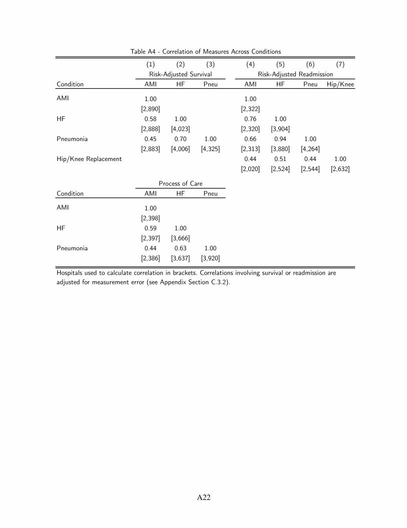
(1) (2) (3) (4) (5) (6) (7)
Condition AMI HF Pneu AMI HF Pneu Hip/Knee
AMI 1.00 1.00
[2,890] [2,322]
HF 0.58 1.00 0.76 1.00
[2,888] [4,023] [2,320] [3,904]
Pneumonia 0.45 0.70 1.00 0.66 0.94 1.00
[2,883] [4,006] [4,325] [2,313] [3,880] [4,264]
Hip/Knee Replacement 0.44 0.51 0.44 1.00
[2,020] [2,524] [2,544] [2,632]
Condition AMI HF Pneu
AMI 1.00
[2,398]
HF 0.59 1.00
[2,397] [3,666]
Pneumonia 0.44 0.63 1.00
[2,386] [3,637] [3,920]
Table A4 - Correlation of Measures Across Conditions
Risk-Adjusted Survival Risk-Adjusted Readmission
Hospitals used to calculate correlation in brackets. Correlations involving survival or readmission are
adjusted for measurement error (see Appendix Section C.3.2).
Process of Care
A22

(1) (2) (3) (4)
Measure \ Condition AMI HF Pneu Hip/Knee
Risk-Adjusted Survival 0.19 0.21 0.17
[198] [274] [289]
Risk-Adjusted Readmission 0.09 -0.09 0.45 0.21
[158] [267] [288] [190]
Process of Care Z-Score 0.12 0.35 0.28
[162] [244] [263]
Patient Survey Z-Score -0.01 -0.02 -0.02 0.05
[227] [233] [233] [202]
Each cell shows the correlation between our measure and the Bloom-
Van Reenen average management score at the hospital. Hospitals
used to calculate correlation in brackets. Correlations involving
survival or readmission are adjusted for measurement error (see
Appendix Section C.3.2).
Table A5 - Correlation of Management Scores and Quality
(1) (2) (3) (4) (5) (6) (7) (8)
Measure \ Condition AMI HF Pneu Hip/Knee AMI HF Pneu Hip/Knee
Risk-Adjusted Survival 12.866 17.839 4.237 0.217 1.827 1.269
(1.421) (1.902) (0.764) (0.600) (0.586) (0.357)
Risk-Adjusted Readmission -6.108 -14.155 -1.120 -20.716 -0.814 -2.264 -0.580 -0.757
(1.983) (2.214) (1.552) (2.108) (0.745) (0.668) (0.644) (0.845)
Process of Care Z-Score 0.196 0.188 0.196 0.036 0.014 0.015
(0.027) (0.022) (0.014) (0.011) (0.010) (0.009)
Patient Survey Z-Score -0.113 -0.292 -0.166 -0.022 0.002 -0.014 -0.004 0.025
(0.040) (0.028) (0.022) (0.034) (0.013) (0.009) (0.009) (0.016)
Hospitals 2,193 3,316 3,454 2,542 2,193 3,316 3,454 2,542
Table A6 - Allocation across Conditions - Multivariate Approach to Measuring Quality
Static Allocation Dynamic Allocation
This table repeats the analysis of Table 4 but uses all available quality measures for the condition at once (plus the
patient survey, which is not condition-specific). The allocation sample for each regression is all hospitals with the
displayed quality measures and at least one patient in 2008. Standard errors are bootstrapped with 300 replications
and are clustered at the market level.
A23

(1) (2) (3) (4) (5) (6) (7) (8)
Measure \ Condition AMI HF Pneu Hip/Knee AMI HF Pneu Hip/Knee
Risk-Adjusted Survival 12.082 13.870 4.192 0.526 1.364 1.170
(0.929) (1.296) (0.745) (0.401) (0.452) (0.323)
Hospitals 2,193 3,316 3,454 2,193 3,316 3,454
Risk-Adjusted Readmission -9.909 -10.519 -1.372 -20.742 -1.127 -1.969 -0.733 -0.988
(1.600) (1.686) (1.562) (2.097) (0.567) (0.531) (0.561) (0.835)
Hospitals 2,193 3,316 3,454 2,542 2,193 3,316 3,454 2,542
Process of Care Z-Score 0.327 0.300 0.185 0.045 0.030 0.018
(0.023) (0.018) (0.015) (0.009) (0.008) (0.008)
Hospitals 2,193 3,316 3,454 2,193 3,316 3,454
Patient Survey Z-Score 0.074 -0.172 -0.121 0.068 0.017 0.004 0.004 0.029
(0.030) (0.031) (0.028) (0.035) (0.012) (0.007) (0.008) (0.015)
Hospitals 2,193 3,316 3,454 2,542 2,193 3,316 3,454 2,542
Table A7 - Allocation across Conditions - Constant Sample
Static Allocation Dynamic Allocation
This table repeats the analysis of Table 4 but uses a constant sample of hospitals across the quality metrics. The
sample for each regression is all hospitals with a risk-adjusted survival rate (if calculated for that condition), risk-
adjusted readmission rate, process of care score (if calculated for that condition), patient survey score, and at least
one patient in 2008. Standard errors are bootstrapped with 300 replications and are clustered at the market level.
A24

(1) (2) (3) (4) (5) (6) (7) (8)
Measure \ Condition AMI HF Pneu Hip/Knee AMI HF Pneu Hip/Knee
AMI 0.553 0.335 0.183 0.048 0.014 0.031
(0.030) (0.022) (0.021) (0.014) (0.009) (0.010)
HF 0.198 0.124 0.031 -0.001 0.010 0.004
(0.036) (0.030) (0.026) (0.017) (0.011) (0.012)
Pneumonia 0.034 0.080 0.052 0.014 0.010 0.032
(0.034) (0.024) (0.019) (0.014) (0.013) (0.011)
Hospitals 2,882 2,882 2,882 2,882 2,882 2,882
AMI -0.171 -0.112 -0.122 -0.265 -0.031 -0.035 -0.018 -0.001
(0.047) (0.038) (0.035) (0.056) (0.019) (0.014) (0.015) (0.023)
HF -0.215 -0.146 -0.086 -0.282 -0.027 -0.043 -0.028 -0.007
(0.044) (0.031) (0.030) (0.054) (0.019) (0.017) (0.015) (0.021)
Pneumonia 0.104 0.084 0.041 -0.055 -0.006 -0.014 -0.018 -0.008
(0.042) (0.031) (0.027) (0.050) (0.019) (0.017) (0.015) (0.024)
Hip/Knee Replacement -0.079 -0.067 -0.086 -0.284 -0.010 -0.016 0.002 -0.024
(0.034) (0.024) (0.021) (0.041) (0.013) (0.012) (0.012) (0.016)
Hospitals 2,018 2,018 2,018 2,018 2,018 2,018 2,018 2,018
AMI 0.336 0.209 0.165 0.058 0.046 0.014
(0.031) (0.021) (0.020) (0.013) (0.011) (0.011)
HF -0.054 -0.103 -0.219 -0.061 -0.027 0.001
(0.049) (0.040) (0.042) (0.025) (0.020) (0.018)
Pneumonia 0.001 0.094 0.205 0.036 0.026 0.025
(0.051) (0.041) (0.037) (0.020) (0.020) (0.016)
Hospitals 2,386 2,389 2,390 2,386 2,389 2,390
This table repeats the analyses of Table 4 but rather than using the one (non-standardized, except for process of
care) quality measure for the left-hand side condition, it uses Z-scores of all condition specific quality measures.
Each column in a panel represents one regression, e.g. the top panel of column (1) regresses hospital size for AMI
on risk-adjusted survival Z-scores for AMI, HF, and pneumonia. Standard errors are analytic and clustered at the
market level.
Table A8 - Allocation with Respect to All Condition-Specific Quality Measures
Static Allocation Dynamic Allocation
Risk-Adjusted Survival Z-Score
Risk-Adjusted Readmission Z-Score
Process of Care Z-Score
A25

(1) (2) (3) (4) (5) (6) (7) (8)
Condition
Measure \ Model Baseline Poisson Baseline Poisson Baseline Poisson Baseline Poisson
Risk-Adjusted Survival 17.496 18.631 15.360 17.532 5.140 6.478
(0.995) (1.109) (1.320) (1.504) (0.777) (0.829)
Hospitals 2,890 2,881 4,023 4,023 4,325 4,325
Risk-Adjusted Readmission -9.162 -10.685 -10.346 -13.145 0.499 -1.922 -21.037 -25.811
(1.621) (2.086) (1.782) (2.175) (1.575) (1.756) (2.027) (3.466)
Hospitals 2,322 2,304 3,904 3,903 4,264 4,264 2,632 2,626
Process of Care Z-Score 0.319 0.422 0.332 0.332 0.211 0.199
(0.026) (0.024) (0.016) (0.020) (0.015) (0.014)
Hospitals 2,398 2,379 3,666 3,665 3,920 3,920
Patient Survey Z-Score -0.321 -0.131 -0.252 -0.123 -0.210 -0.114 0.057 0.130
(0.052) (0.035) (0.038) (0.030) (0.030) (0.023) (0.051) (0.057)
Hospitals 3,498 3,498 3,598 3,598 3,610 3,610 3,061 3,059
This table shows the baseline static allocation results of Table 4 in comparison to the same model run as a fixed
effects Poisson regression. To make the models analogous, the Poisson regressand is the count of patients, not its
logarithm. Standard errors are bootstrapped with 300 replications and are clustered at the market level.
The baseline sample is used; hospital counts can be smaller for the Poisson models because they exclude markets
with only one hospital.
Table A9 - Sensitivity of Static Allocation to Poisson Regression Model
AMI HF Pneumonia Hip/Knee
A26

(1) (2) (3) (4) (5) (6) (7) (8)
Condition AMI HF Pneu Hip/Knee AMI HF Pneu Hip/Knee
Baseline Risk-Adjustment 17.496 15.360 5.140 1.533 0.774 1.220
(0.995) (1.320) (0.777) (0.379) (0.501) (0.354)
Age/Race/Sex Only 16.898 14.798 3.209 1.565 0.654 1.065
(0.847) (1.377) (0.764) (0.337) (0.508) (0.361)
No Risk Adjustment 14.896 13.763 3.625 1.520 0.765 1.315
(0.571) (1.192) (0.713) (0.241) (0.420) (0.332)
Hospitals 2,890 4,023 4,325 2,890 4,023 4,325
Baseline Risk-Adjustment -9.162 -10.346 0.499 -21.037 -1.428 -2.300 -1.138 -1.112
(1.621) (1.782) (1.575) (2.027) (0.611) (0.651) (0.679) (0.836)
Age/Race/Sex Only -10.358 -6.466 3.152 -20.023 -1.556 -1.621 -0.547 -1.048
(1.212) (1.457) (1.280) (1.859) (0.475) (0.528) (0.482) (0.767)
No Risk Adjustment -10.909 -5.596 2.753 -20.710 -1.601 -1.514 -0.585 -1.140
(1.096) (1.441) (1.272) (1.819) (0.435) (0.511) (0.465) (0.732)
Hospitals 2,322 3,904 4,264 2,632 2,322 3,904 4,264 2,632
Table A10 - Sensitivity of Allocation Results to Risk Adjustment
Static Allocation Dynamic Allocation
This table shows the sensitivity of the allocation results of Table 4 to the risk-adjustment procedure. In each panel, we
repeat the baseline allocation results with full risk adjustment, followed by identical specifications under two alternative
measures. First, we risk-adjust using only age-race-sex interactions. Second, we perform no risk-adjustment. Standard errors
are bootstrapped with 300 replications and are clustered at the market level.
Panel A - Risk-Adjusted Survival
Panel B - Risk-Adjusted Readmission
A27

(1) (2) (4) (5) (7) (8) (10) (11)
Condition
Sample Baseline Choice Baseline Choice Baseline Choice Baseline Choice
Share Baseline Patients in Sample 1.00 0.87 1.00 0.89 1.00 0.90 1.00 0.84
Risk-Adjusted Survival 17.496 16.769 15.360 15.184 5.140 5.402
(0.995) (0.988) (1.320) (1.341) (0.777) (0.808)
Hospitals 2,890 2,889 4,023 4,023 4,325 4,324
Risk-Adjusted Readmission -9.162 -9.447 -10.346 -10.561 0.499 -0.233 -21.037 -20.794
(1.621) (1.600) (1.782) (1.823) (1.575) (1.590) (2.027) (2.014)
Hospitals 2,322 2,322 3,904 3,904 4,264 4,263 2,632 2,632
Process of Care Z-Score 0.319 0.317 0.332 0.332 0.211 0.210
(0.026) (0.026) (0.016) (0.016) (0.015) (0.016)
Hospitals 2,398 2,397 3,666 3,662 3,920 3,918
Patient Survey Z-Score -0.321 -0.316 -0.252 -0.261 -0.210 -0.217 0.057 0.041
(0.052) (0.051) (0.038) (0.039) (0.030) (0.030) (0.051) (0.048)
Hospitals 3,498 3,480 3,598 3,594 3,610 3,608 3,061 3,046
This table repeats the static allocation analysis of Table 4 and shows how it is affected by restricting to patients who
were treated in their market of residence, which is the patients who were included in the choice model. For each
condition, the left column (Baseline) repeats our baseline results. The right column (Choice) runs the same regression but
only counts patients residing in the hospital's market. Standard errors are bootstrapped with 300 replications and are
clustered at the market level.
Table A11 - Static Allocation Restricted to Patients Treated in Market of Residence (Choice Model Subsample)
AMI Heart Failure Pneumonia Hip/Knee
A28

(1) (2) (3) (4) (5) (6) (7) (8)
Condition AMI AMI AMI AMI HF HF HF HF
Mean miles to chosen hospital 12.48 12.67 12.65 12.45 8.27 8.27 8.30 8.35
SD miles to chosen hospital 20.06 20.27 20.27 20.31 13.25 13.25 13.27 13.33
Distance -0.111 -0.128 -0.137 -0.099 -0.159 -0.163 -0.160 -0.159
(0.006) (0.007) (0.007) (0.005) (0.006) (0.007) (0.007) (0.007)
Distance2 0.00019 0.00032 0.00034 0.00012 0.00018 0.00026 0.00013 0.00013
(0.00003) (0.00003) (0.00003) (0.00001) (0.00001) (0.00002) (0.00001) (0.00001)
Risk-Adjusted Survival 19.004 16.041
(1.147) (1.728)
Risk-Adjusted Readmission -13.626 -16.491
(2.007) (1.808)
Process of Care Z-Score 0.568 0.353
(0.036) (0.028)
Patient Survey Z-Score -0.031 0.015
(0.037) (0.032)
Patients 165,005 158,086 158,032 167,429 275,671 274,667 270,773 266,915
Observations 2,869,091 2,321,684 2,427,869 3,359,387 6,241,586 6,103,120 5,811,375 5,532,403
Avg Hospital Choices/Patient 17.39 14.69 15.36 20.06 22.64 22.22 21.46 20.73
Table A12 - Choice Model of Patient Allocation - Raw Logit Coefficients
This table shows the raw logit coefficients (log odds ratios) from the models of Table 5. See that table for sample restrictions. Standard
errors are analytic and clustered at the market level.
A29

(9) (10) (11) (12) (13) (14)
Condition Pneu Pneu Pneu Pneu Hip/Knee Hip/Knee
Mean miles to chosen hospital 7.49 7.49 7.50 7.54 13.16 13.09
SD miles to chosen hospital 11.92 11.91 11.77 11.77 18.85 18.80
Distance -0.178 -0.178 -0.181 -0.185 -0.105 -0.101
(0.006) (0.006) (0.006) (0.007) (0.004) (0.004)
Distance2 0.00013 0.00013 0.00013 0.00013 0.00017 0.00012
(0.00001) (0.00001) (0.00001) (0.00001) (0.00002) (0.00001)
Risk-Adjusted Survival 6.647
(0.962)
Risk-Adjusted Readmission -7.927 -24.091
(1.979) (2.570)
Process of Care Z-Score 0.238
(0.018)
Patient Survey Z-Score -0.007 0.157
(0.028) (0.039)
Patients 317,904 317,374 309,623 298,185 222,673 224,451
Observations 7,766,357 7,666,146 6,997,264 6,233,133 3,422,903 4,017,558
Avg Hospital Choices/Patient 24.43 24.15 22.60 20.90 15.37 17.90
Table A12 Continued - Choice Model of Patient Allocation - Raw Logit Coefficients
This table shows the raw logit coefficients (log odds ratios) from the models of Table 5. See that table for sample
restrictions. Standard errors are analytic and clustered at the market level.
A30

(1)
(2)
(3)
(4)
(5)
(6)
(7)
(8)
(9)
(10)
Mea
sure
\ Y
ear
1996
1999
2002
2005
2008
1996
1999
2002
2005
2008
Sta
tic
Allo
cation
11.4
6313
.759
14.2
0116
.082
17.4
962.
741
2.38
91.
118
9.22
215
.360
(0.8
38)
(1.0
08)
(1.0
58)
(0.8
15)
(0.8
24)
(1.1
17)
(1.4
23)
(1.5
80)
(1.3
69)
(1.3
48)
Dyn
amic
Allo
cation
0.53
60.
875
0.78
71.
103
1.53
30.
609
-0.0
950.
580
0.83
90.
774
(0.3
41)
(0.4
75)
(0.4
22)
(0.3
22)
(0.3
80)
(0.5
25)
(0.5
44)
(0.5
96)
(0.4
20)
(0.4
83)
Hos
pital
s3,
708
3,55
83,
487
3,26
72,
890
4,36
14,
254
4,17
64,
130
4,02
3
Mea
sure
\ Y
ear
1996
1999
2002
2005
2008
Sta
tic
Allo
cation
-2.4
23-2
.723
-2.6
903.
763
5.14
0
(0.7
50)
(0.7
78)
(0.8
45)
(0.8
00)
(0.7
68)
Dyn
amic
Allo
cation
-0.1
43-0
.608
0.18
1-0
.124
1.22
0
(0.3
14)
(0.3
65)
(0.2
88)
(0.3
31)
(0.3
63)
Hos
pital
s4,
565
4,49
64,
403
4,37
54,
325
Tab
le A
13 - S
tatic
and D
ynam
ic A
lloca
tion
ove
r T
ime
This t
able
show
s th
e al
loca
tion
rel
atio
nsh
ips
with r
espec
t to
risk-
adju
sted
surv
ival
ove
r tim
e. R
isk-
adju
sted
surv
ival
is
calc
ula
ted fro
m a
regr
ession
of su
rviv
al o
n h
ospital
fix
ed e
ffec
ts a
nd p
atie
nt
risk
-adju
ster
s. A
sep
arat
e re
gres
sion
is
run for
eac
h o
f th
e ye
ar g
roups
1994
-
1996
, 19
97-1
999,
200
0-20
02, 20
03-2
005,
and 2
006-
2008
. T
he
empiric
al-B
ayes
-adju
sted
hos
pital
effec
ts a
re c
onsider
ed t
he
hos
pital
's
qual
ity
met
ric
for
the
year
gro
up's t
erm
inal
yea
r, t
he
stat
ic a
lloca
tion
anal
ysis is
bas
ed o
n p
atie
nt
allo
cation
in t
he
term
inal
yea
r, a
nd t
he
dyn
amic
allo
cation
is
bas
ed o
n g
row
th b
etwee
n t
he
term
inal
yea
r an
d t
he
subse
quen
t 2
year
s. T
hus, for
exa
mple
, th
e "1
996"
anal
ysis
mea
sure
s qual
ity
over
199
4-19
96, st
atic
allo
cation
in 1
996,
and d
ynam
ic a
lloca
tion
bas
ed o
n g
row
th b
etwee
n 1
996
and 1
998.
Sta
ndar
d
erro
rs a
re a
nal
ytic
and c
lust
ered
at
the
mar
ket
leve
l.
AM
IH
F
Pneu
mon
ia
A31

(1) (2) (3) (4) (5) (6)
Measure \ Condition AMI HF Pneu AMI HF Pneu
Risk-Adjusted Survival 14.840 19.870 3.440 5.381 -0.125 0.637
(1.215) (2.093) (1.159) (1.071) (0.993) (0.720)
Hospitals 2,879 4,023 4,325 2,320 3,924 4,246
Risk-Adjusted Readmission -6.086 -17.273 -3.285 -6.180 -0.828 0.330
(3.831) (2.469) (1.900) (1.695) (1.324) (1.173)
Hospitals 2,302 3,903 4,264 1,953 3,811 4,191
Process of Care Z-Score 0.317 0.173 0.015 0.151 0.038 0.023
(0.046) (0.018) (0.017) (0.028) (0.015) (0.012)
Hospitals 2,377 3,665 3,920 1,944 3,541 3,819
Patient Survey Z-Score -0.039 -0.057 0.001 -0.103 0.001 -0.001
(0.037) (0.027) (0.023) (0.035) (0.020) (0.018)
Hospitals 3,498 3,598 3,610 2,653 3,472 3,513
Table A14 - Allocation for Non-ED Non-Transfer Patients across Conditions
Static Allocation Dynamic Allocation
This table repeats the analysis of Table 4 but considers hospital size and growth counting only
non-ED non-transfer patients (the omitted category of patients from the analysis of Table 9).
Static allocation uses the Poisson model (see Appendix Table A9) and the baseline allocation
sample. Dynamic allocation uses the subset of hospitals with at least one non-ED non-transfer
patient in 2008. Standard errors are bootstrapped with 300 replications and are clustered at
the market level.
A32

(1) (2) (3) (4) (5) (6)
Condition
Source of Admission ED Transfer ED Transfer ED Transfer
Baseline Static Allocation 14.377 29.264 15.254 24.036 7.720 5.658
(0.878) (2.184) (1.693) (2.566) (1.387) (1.658)
P-value of test for equality
Hospitals 2,742 1,408 3,329 1,563 3,513 1,601
Poisson Static Allocation 14.489 42.532 15.727 50.673 7.168 14.049
(1.022) (2.609) (1.586) (4.664) (0.983) (2.941)
P-value of test for equality
Hospitals 2,881 2,881 4,023 4,011 4,325 4,275
Baseline Static Allocation -7.903 -13.315 -10.690 -16.527 0.204 2.008
(1.295) (3.904) (1.775) (3.483) (2.314) (3.107)
P-value of test for equality
Hospitals 2,276 1,361 3,277 1,550 3,488 1,592
Poisson Static Allocation -8.128 -25.550 -11.265 -37.988 -1.647 1.089
(1.730) (5.921) (2.329) (6.744) (2.021) (6.252)
P-value of test for equality
Hospitals 2,304 2,304 3,903 3,892 4,264 4,214
Baseline Static Allocation 0.272 0.874 0.370 0.325 0.307 0.078
(0.023) (0.062) (0.024) (0.036) (0.030) (0.035)
P-value of test for equality
Hospitals 2,369 1,376 3,245 1,520 3,389 1,548
Poisson Static Allocation 0.326 1.179 0.377 0.754 0.262 0.214
(0.021) (0.090) (0.025) (0.058) (0.018) (0.043)
P-value of test for equality
Hospitals 2,379 2,379 3,665 3,653 3,920 3,869
Baseline Static Allocation -0.234 0.232 -0.227 0.045 -0.218 -0.087
(0.049) (0.067) (0.041) (0.046) (0.041) (0.039)
P-value of test for equality
Hospitals 3,116 1,438 3,214 1,496 3,257 1,484
Poisson Static Allocation -0.157 -0.034 -0.141 -0.090 -0.137 -0.203
(0.035) (0.072) (0.032) (0.060) (0.028) (0.057)
P-value of test for equality
Hospitals 3,498 3,498 3,598 3,586 3,610 3,559
This table shows the static allocation results for ED and non-ED transferred patients using Poisson
regression (as in Table 9) and linear regression. The left hand side of these regressions considers hospital
size counting only ED patients in the odd-numbered columns and only non-ED transferred patients in the
even-numbered columns. To make the linear and Poisson models analogous, the Poisson regressand is the
count of patients, not its logarithm. Both approaches include market fixed effects. Hospital counts can be
smaller for the Poisson models because they exclude markets with only one hospital. In addition, in the
Poisson models, hospital counts may differ between ED and non-ED transfers for the same condition and
quality measure because the counts also exclude markets with no variation in the outcome (e.g. all zeroes).
Standard errors are bootstrapped with 300 replications and are clustered at the market level.
0.261
Patient Survey Z-Score
0.051 0.349 0.170
0.000 0.000 0.008
Process of Care Z-Score
0.000 0.233 0.000
0.000 0.000
0.001 0.000 0.653
0.000 0.001 0.222
0.000 0.000 0.009
Risk-Adjusted Readmission
0.109 0.062 0.585
Risk-Adjusted Survival
Table A15 - Sensitivity of ED and Non-ED Transfer Patient Static Allocation to Poisson Regression Model
AMI Heart Failure Pneumonia
A33

(1) (2) (3) (4) (5) (6)
Condition
Source of Admission ED Transfer ED Transfer ED Transfer
Share of patients in 2008 0.79 0.14 0.76 0.02 0.77 0.01
Median miles to chosen hospital 4.7 29.8 4.4 26.3 4.4 21.1
Mean miles to chosen hospital 8.2 36.8 7.1 32.3 7.1 27.7
Share treated at nearest hospital 0.57 0.04 0.58 0.09 0.60 0.15
MRS(1 pp risk-adjusted survival, miles) -0.744 -16.061 -0.623 -16.642 -0.317 -4.014
(0.075) (1.423) (0.103) (1.601) (0.054) (0.777)
P-value of test for equality
Patients 129,889 23,185 209,094 6,130 244,358 4,097
MRS(1 pp risk-adjusted readmission, miles) 0.527 10.818 0.734 12.774 0.410 1.303
(0.086) (2.097) (0.104) (2.193) (0.102) (1.713)
P-value of test for equality
Patients 124,707 22,947 208,842 6,115 244,181 4,088
MRS(1 SD process of care, miles) -2.024 -36.431 -1.712 -25.332 -1.392 -6.321
(0.191) (3.468) (0.212) (2.521) (0.122) (1.545)
P-value of test for equality
Patients 124,989 22,913 208,503 6,083 243,368 4,025
MRS(1 SD patient survey, miles) -0.052 0.090 -0.179 2.178 -0.024 4.896
(0.217) (3.591) (0.172) (2.092) (0.144) (1.682)
P-value of test for equality
Patients 131,603 23,281 207,472 6,059 241,158 3,948
Distance MRSs were evaluated at 12.48 12.48 8.27 8.27 7.49 7.49
Table A16 - Choice Model of Patient Allocation for ED and Non-ED Transfer Patients across Conditions
These regressions repeat the conditional logit choice models of Table 5 but are restricted to ED patients (in odd
columns) and non-ED transfer patients (in even columns). Standard errors are analytic and clustered at the market
level.
This table reports the marginal rates of substitution (MRSs) of quality for distance derived from the conditional logit
model (see equation 6). For the survival and readmission rates, the MRS given by equation (6) is divided by 100 to
put it into percentage point terms. MRSs for a condition are evaluated at the same distance that was used for the
condition in Table 5.
The sample is ED patients (odd columns) or non-ED transfer patients (even columns) with the condition in 2008 who
stayed in their market of residence for treatment. The choice set for a patient is all hospitals in his market with the
quality measure available that treated at least one patient in 2008.
AMI Heart Failure Pneumonia
0.000 0.000 0.001
0.000 0.000 0.000
0.000 0.000 0.598
Risk-Adjusted Survival
Risk-Adjusted Readmission
Process of Care Z-Score
Patient Survey Z-Score
0.968 0.250 0.002
A34

(1) (2) (3) (4) (5) (6) (7) (8)
Condition
Measure \ Method Baseline Mech Baseline Mech Baseline Mech Baseline Mech
Share truly going to closest
Risk-Adjusted Survival 17.496 2.309 15.360 2.507 5.140 0.685
(0.995) (0.577) (1.320) (1.115) (0.777) (0.653)
Hospitals 2,890 2,888 4,023 4,021 4,325 4,322
Risk-Adjusted Readmission -9.162 -0.470 -10.346 -0.660 0.499 -0.328 -21.037 -2.783
(1.621) (1.111) (1.782) (1.305) (1.575) (1.130) (2.027) (1.140)
Hospitals 2,322 2,320 3,904 3,902 4,264 4,261 2,632 2,630
Process of Care Z-Score 0.319 0.018 0.332 0.158 0.211 0.099
(0.026) (0.015) (0.016) (0.012) (0.015) (0.010)
Hospitals 2,398 2,396 3,666 3,664 3,920 3,918
Patient Survey Z-Score -0.321 -0.203 -0.252 -0.238 -0.210 -0.182 0.057 -0.101
(0.052) (0.024) (0.038) (0.023) (0.030) (0.021) (0.051) (0.018)
Hospitals 3,498 3,496 3,598 3,595 3,610 3,607 3,061 3,058
Table A17 - Static Allocation with Patients Mechanically Allocated to Nearest Hospital
This table shows our baseline static allocation results from Table 4 in comparison to an alternative allocation
constructed by mechanically assigning each patient to his closest hospital. Only hospitals that treated at least
one patient with the condition in 2008 are eligible for mechanical assignment. Distance is measured from the
ZIP code centroid of the patient's residence to the ZIP code centroid of the hospital. The sample for each
regression is all hospitals with the relevant quality measure and at least one mechanically allocated patient in
2008. Standard errors are bootstrapped with 300 replications and are clustered at the market level.
AMI HF Pneumonia Hip/Knee
0.44 0.52 0.56 0.38
A35

(1) (2) (3) (4) (5) (6) (7) (8)
Condition
Measure \ Method Baseline Mech Baseline Mech Baseline Mech Baseline Mech
Share truly going to closest
Risk-Adjusted Survival 1.533 -0.297 0.774 0.378 1.220 0.842
(0.379) (0.250) (0.501) (0.497) (0.354) (0.356)
Hospitals 2,890 2,888 4,023 4,021 4,325 4,322
Risk-Adjusted Readmission -1.428 -0.076 -2.300 -1.358 -1.138 -0.988 -1.112 -0.378
(0.611) (0.585) (0.651) (0.565) (0.679) (0.562) (0.836) (0.747)
Hospitals 2,322 2,320 3,904 3,902 4,264 4,261 2,632 2,630
Process of Care Z-Score 0.048 0.015 0.043 0.027 0.026 0.019
(0.010) (0.010) (0.009) (0.008) (0.009) (0.009)
Hospitals 2,398 2,396 3,666 3,664 3,920 3,918
Patient Survey Z-Score -0.065 -0.041 -0.003 0.000 0.007 -0.004 0.037 0.014
(0.015) (0.012) (0.011) (0.009) (0.011) (0.008) (0.022) (0.016)
Hospitals 3,498 3,496 3,598 3,595 3,610 3,607 3,061 3,058
This table shows our baseline dynamic allocation results from Table 4 in comparison to an alternative
allocation constructed by mechanically assigning each patient to his closest hospital. Only hospitals that
treated at least one patient with the condition in 2008 are eligible for mechanical assignment. Distance is
measured from the ZIP code centroid of the patient's residence to the ZIP code centroid of the hospital. The
sample for each regression is all hospitals with the relevant quality measure and at least one mechanically
allocated patient in 2008. Standard errors are bootstrapped with 300 replications and are clustered at the
market level.
Table A18 - Dynamic Allocation with Patients Mechanically Allocated to Nearest Hospital
AMI HF Pneumonia Hip/Knee
0.44 0.52 0.56 0.38
A36

(1) (2) (3)
Measure \ Condition AMI HF Pneu
Risk-Adjusted Mortality 0.79 0.73 0.82
[2,802] [3,788] [3,994]
Risk-Adjusted Readmission 0.66 0.67 0.71
[2,254] [3,681] [3,924]
Table A19 - Correlation with CMS Quality Measures
Each cell shows the correlation between our 2008 empirical-
Bayes-adjusted quality measure and the CMS 2008 risk-
standardized quality measure. We produce our risk-adjusted
survival measure as risk-adjusted mortality to match the
CMS measure. Hospitals used to calculate correlation in
brackets.
A37