Embed Size (px)
Citation preview

MASTER THESIS
Head top detection using
3D-information from multiple cameras
Hung Nguyen Department of Signals and Systems Division of Automatic Control, Automation and Mechatronics Chalmers University of Technology Gothenburg, 2012

Abstract Human tracking has been a challenging task in computer vision for a long time. One common
problem faced when accepting this task is occlusions which makes body segmentation difficult. In
recent years algorithms have been developed using multiple cameras facing the tracking scene from
different angles to overcome the occlusion problems. In this project one of these algorithms has
been studied to find its strengths and weaknesses. Some modifications have also been applied to the
algorithm to see if it can be improved. The algorithm is focused on detecting head tops so the
cameras are placed at high elevation aiming downwards towards the tracking area. By setting up the
cameras in this way the head tops are most likely to always be visible. The algorithm extracts height
information by combining the data from the different cameras. The frames from the different views
are transformed using planar homography to align the head tops in all the views. And through
intensity correlation between pixels in the different views the head tops are then detected. The
algorithm was tested in an outdoor environment on still images to test the detection part of the
algorithm. The tracking part was not tested. Experiments showed that the modification improved the
results but at the expense of calculation time.

Contents Abstract ..............................................................................................................................................1
1 Introduction ................................................................................................................................1
1.1 Purpose ...............................................................................................................................1
1.2 Objective .............................................................................................................................1
1.3 Problem formulation ...........................................................................................................1
1.4 Related work .......................................................................................................................1
1.5 Structure of the thesis .........................................................................................................2
2 Theory ........................................................................................................................................3
2.1 Planar homographic transformation ....................................................................................3
2.1.1 Direct linear transformation (DLT) algorithm ................................................................4
2.2 Homography calculation between views ..............................................................................5
3 Method .......................................................................................................................................7
3.1 Background subtraction .......................................................................................................7
3.1.1 Background subtraction using homography .................................................................8
3.2 Head top detection ..............................................................................................................9
3.2.1 Background subtraction ...............................................................................................9
3.2.2 Homographic transformation ..................................................................................... 10
3.2.3 Pixel matching ........................................................................................................... 10
3.2.4 2D patch clustering .................................................................................................... 10
4 Experimental results ................................................................................................................. 11
4.1 The setup .......................................................................................................................... 11
4.2 Background subtraction ..................................................................................................... 11
4.3 Head top alignment ........................................................................................................... 14
4.4 Pixel matching ................................................................................................................... 15
4.5 Grayscale vs RGB correlation analysis ................................................................................ 19
4.6 Discussion ......................................................................................................................... 20
5 Conclusion ................................................................................................................................ 21
References ..........................................................................................................................................0

1
1 Introduction In crowded areas such as subways, supermarkets or exhibitions there is an interest in understanding
the behavior of how the crowd is moving and how the individuals in the crowd are moving. At
subway, tram or bus stations, transports could be better scheduled if we knew more about how the
travellers are moving at the station. The configuration of stops for large stations with many lines
intersecting is not trivial. With more information about how the travellers are moving between stops
to change lines, the configuration of which line to stop at which stop could be better optimized. This
information may also be useful when designing new large stations to avoid configurations that may
cause bottlenecks.
When looking at the crowd in a supermarket interest may be focused on identifying attractive
regions in order to sell more products. In a grocery store we may see that some shelves or products
may draw the customer’s attention more than others. Another interesting thing is the route that the
customers are taking through the store. If this information can be extracted, shelves and products
can be strategically placed to sell more and to optimize evacuation conditions if an accident would
occur. The same thing goes for an exhibition were the stands have to be placed carefully so that
evacuation is not hindered. Also at an exhibition it might be interesting to know how often different
stands were visited. The need for this kind of information is the background of this thesis, which will
present a method for gathering position data of people moving in an observation area.
1.1 Purpose The purpose is to gather information about how the individuals in a crowd are moving in e.g. a
supermarket or an exhibition. The information can be used to detect bottlenecks, movement
patterns and identify more or less attractive regions for stand and shelf placement and to optimize
evacuation.
1.2 Objective The aim of this project is to design a system that collects position data of individuals in a crowd. The
idea is to use multiple cameras with overlapping fields of view mounted on the ceiling of the
observation area. Instead of using the image of just one camera, two or more cameras will be used to
extract depth information from the images. Object identification will then be partially based on the
depth information of the images.
1.3 Problem formulation This is a thesis on an old problem in image processing. It is usually referred to as human tracking or
human crowd tracking. The problem is to design a system which can recognize people and distinguish
between people in a dense crowd. After recognition it also has to track the person that it has
recognized. The common problem in designing such a system is that it is very hard to distinguish
between different people in a crowd due to occlusions. This makes it hard to detect all persons in the
crowd and in the tracking phase it hard to keep track of the same person.
1.4 Related work A literature study has been made and the ideas and methods for solving this task have been inspired
by previous work. A few of these are presented here. They are all based on a multiple camera system
and the last presented is the one which this method is mostly based on.

2
Keck, Davis and Tyagi (2006) presented a method which used epipolar geometry between the
cameras to reconstruct 3D points of the tracking scene. People in the scene would be detected as
clouds of 3D points and to identify one object in the scene the 3D points are merged into clusters to
form single objects. The problem with this method is that if the scene is very crowded the 3D point
clouds from many people will merge and it will be hard to distinguish between many persons.
Garibotto and Cibei (2005) presented a method based on binocular stereovision. It uses
homographies of parallel planes at multiple heights to scan through the observation area and
completely reconstruct the objects in the observation area unlike Keck, Davis and Tyagi who are only
reconstructing the objects as clouds. The method does not include any mechanism for handling
occlusions which makes the method only feasible for areas with very few people.
Kobayashi et al. (2006) are using a method based on appearance and features of the head to track
the head of a person. The multiple cameras make it possible to catch those features from different
angles so that it won’t matter how the person is oriented in the scene. But this method could only
track one person.
Du and Piater (2007) track targets in different cameras separately by using particle filters. The results
are then combined in another particle filter on the ground plane to track the people’s feet. The
problem with this method is the dependence on the tracker of each camera which cannot handle
occlusions well.
Khan and Shah (2006) used a method to track the feet of the persons in the tracking scene. This is
done by using the homography of the ground plane. The homography transforms the frames in the
different camera views so that the ground plane is aligning in all the views. So the feet which are on
the ground plane will also align. The algorithm detects the feet by searching for alignment of
foreground. The problems encountered are shadows which are not always subtracted and will
disturb the process. Also when the scene is very crowded some feet will be totally occluded and
unable to detect.
The next method that is presented is the one that this project is mostly based on. It is presented by
Eshel and Moses (2010) and like Khan and Shah it also uses homography. The method is also aligning
foreground pixels like Khan and Shah but instead of tracking feet this method is tracking head tops so
the homography is made on planes at head heights instead of the ground plane. It also uses intensity
correlation to match the head tops in the different views unlike Khan and Shah who are only
distinguishing between background and foreground pixels. The method works quite well even in very
crowded scenes since head tops are almost always visible if the cameras are placed at a high
elevation. One problem is that the system sometimes produces false detections, that is, the system
detects head tops where there actually are no head tops.
1.5 Structure of the thesis This thesis will present a method for detecting head tops and the location of the head top. The
method that is being presented is much like the method presented by Eshel and Moses but some
modifications have been done.
The thesis starts off with a theory section describing homography and how multiple height
homographies have been calculated for the method being presented. In section 3 the method is

3
being presented. Section 3.1 describes the method used to subtract the background and section 3.2
presents the head top detection algorithm. In section 4 the experiments and the results are
presented. Finally the results are discussed in section 4.6 and conclusions are drawn in section 5.
2 Theory This section describes the theory behind one important building block of this project, namely
homography.
2.1 Planar homographic transformation A homography is an invertible transformation from a projective space to itself that maps straight
lines to straight lines. It preserves incidence and cross-ratio but not angles or sizes.
In this project we use homography to process the gathered information from the different cameras.
It describes how the points on a plane are perceived when the angle of view is changing. In our case,
how the pixels on a plane are changing when viewed from the different camera angles. The figure
below gives an example of how homography could be used.
In Figure 1, images (a) and (b) show the same scene from two different camera views. Image (c) is a
transformation of image (a), thus only containing pixel information from (a). The transformation is
made such that the ground plane of (c) is aligned with the ground plane of (b). Image (d) shows (b)
and (c) combined to show the alignment of the ground plane. It is seen that the shadows are aligned
but not the persons or the objects in the scene. It is hard to tell if the shrubbery is aligned by looking
Figure 1. Example of homography application. Alignment of the ground plane.
(b) (a)
(c) (d)

4
at the picture but it is actually not. The homography will only align pixels that lie on the same plane
everything else will get shifted.
The example above used the homography of the ground plane from figure 1a and figure 1b. The
method used in this project for calculating such homographies is presented in the next section. It has
been presented by Hartley and Zisserman (2003).
2.1.1 Direct linear transformation (DLT) algorithm
The homography transforms the point to another point by the equation
Where is a 3x3-matrix and and are points represented in homogeneous coordinates. To
represent a 2D-point in homogenous coordinates three parameters are needed and a point will
therefore be a vector consisting of three entities. For more information about homogenous vectors
see Hartley and Zisserman (2003). To determine the homography , of a plane between two views,
four point correspondences on that plane, , are needed. The 3-vectors and are not
necessarily equal since they are homogeneous vectors. They have the same direction but may differ
in magnitude by a nonzero scale factor. To enable a simple linear solution of H to be derived the
equation can be rewritten as the cross product of the two vectors.
If we denote the j-th row of the matrix H by , we can write
(
)
Writing in its homogeneous coordinates as
, the cross product can be rewritten
as
(
)
This gives us a set of three equations in the entries of H, and since for j=1,..,3 we may
write it in matrix form as
*
+
⏟
(
+⏟
is 3x9-matrix and is a 9-vector containing the elements of the -matrix
(
+ [
]

5
where is the j-th element of .
Only two of the equations are linearly independent so the third row is omitted, which gives,
[
] (
+
With four point correspondences we have eight independent equations, and a homogeneous
solution can be calculated for . That is, the solution is determined only up to scale. Since the
solution is determined only up to scale, one entry in may be chosen as .
With the condition that one entry in is equal to 1 there will be eight equations and eight entries to
be determined, which gives an inhomogeneous solution. We chose which gives us
[
] (
*
where is a column vector containing .
Note that if the true solution in fact would be or near zero, there will be no multipliable scale,
, such that and no solution can be reached. But this will only occur for special camera
angles and planes which will not be a problem for this application. It should also be noted that in
order for the plane, that the four point correspondences are lying on, to align in the two views. The
mapping of the camera has to map pictures according to the pinhole model or at least not deviate
too much from it.
2.2 Homography calculation between views This chapter will describe how the homographies used in the head top detection algorithm is
calculated. It has already been described in the previous section that four corresponding points in
each picture are needed to calculate a homography. The head top detection algorithm needs
homographies of planes parallel to the ground at several heights. This chapter will show how to
calculate homographies for arbitrary heights.
If three points on a vertical straight line are known and the heights of these points are known it is
possible to determine a point at an arbitrary height on this line. This is true if the mapping of the
picture is mapped according to the pinhole model. This has already been assumed to be able to use
homographic transformation. In this project we have used a setup to extract these three points. The
setup is shown in Figure 2.

6
Three points on each rod is extracted manually. We could let these points be extracted automatically
by a program by having the points coloured in very strong colours compared to the rest of the scene
or using LEDs with different flash patterns to identify the points. The method with LEDs has been
used by Eshel and Moses. But for the experiments in this project where only stills where used the
easiest solution was to extract the points manually.
Let us call the three points h, m and l for high, medium and low
respectively, see figure. Where h, m and l are their heights over the
ground. We call the projection of these points on the image plane
H, M and L. The projection of a point x at an arbitrary height on the
pole can now be computed by the fact that cross ratios between
distances in the world coordinates is preserved in the image
projection.
In the first step we calculate a cross ratio with the known heights.
This ratio is the same for the distances between the points in the
projected image plane. We can write the corresponding equation
for the distances in the image plane.
where XL stands for the distance between the point X and point L in the image plane, and so on.
In the equation for the aspect ratio in the image plane the unknowns are XL and XM, but
(b) (a)
Figure 2. Figure 2b shows a rod marked up with blue and white stripes where the length of each stripe is 5cm. Figure 2a shows a setup with four of these rods since four points are needed to determine a plane in a picture.
Figure 3. Extracted points on the rod.

7
so we can eliminate XM by inserting
which gives
From this we extract XL to get
XL is the distance between X and L. To get the point X the direction vector from L to X is needed. The
points H and L can be used to calculate the direction vector since X lies on the line between these
two points.
Since this finally gives
This is repeated for all the four rods and for the same heights to get four points on a plane parallel to
the ground. The homography is then calculated using the four points and the method described in
the section 2.1.1.
3 Method This section presents the head top detection algorithm. First a background subtraction algorithm is
presented. This algorithm is also used in the head top detection algorithm which is presented in
section 3.2. The difference between this method and Eshel and Moses method is that a different
background subtractor is used and that the images are analyzed in RGB instead of grayscale.
3.1 Background subtraction In this section a background subtraction method which utilizes the multiple camera system is
presented. The method uses homography to match planes in the background from different camera
views. Other techniques for background subtraction involve comparing the current frame with a
frame taken from an earlier time when the scene only contained the background. A problem with
this approach is that it uses a static reference frame to compare with the current frame. This means
that if the background changes, the results deteriorate. Changes in the background may happen
when lightning conditions change or when objects in the scene are moved. This method will not have
a static reference frame. Instead it will have co-temporal frames from different cameras, that is,
frames taken at the same time. It will have updated frames so changes in the background will not

8
affect this method. A drawback of this method is that it can only remove planes in the background
and it also needs the homography of that plane.
3.1.1 Background subtraction using homography
The example in the theory section, section 2.1, shows how the ground plane can be aligned with the
ground plane in other views by using homography. This method is using this to determine which
pixels that are pixels of the ground. It is using two or more camera views to determine the
background. It needs the homography of the ground plane in the two views if only two cameras are
used. If n views are used there will be n-1 homographic transformations, where each transformation
is from different views to the one view where the background is to be subtracted. The transformed
views will then function as reference views when subtracting the background.
After transforming all the views to one view so that the ground plane in all views are aligned a
matching process is executed. The matching process is looping through all the pixels in the image of
the view where the ground is to be subtracted; we will call this the main view. For every pixel it is
calculating the difference, , between the pixel and the pixel in the other views at the same pixel
coordinate.
| |
Where x and y are the coordinates of the pixel, is the pixel in the main view and is the pixel
in the i:th view. If the difference is lower than a predefined threshold, , the pixel is defined as a
ground plane pixel. For RGB-valued pixels a vector difference is calculated but for a grayscale image
only a scalar difference is calculated.
*
+ [
]
When n views are used the pixel difference is calculated between all views compared to the one view
which we want to background subtract. If any of the differences is below the threshold this pixel is
set as a background pixel i.e. all differences does not have to be below the threshold.
This is because in one view this part of the ground plane may be occluded by the foreground but not
in another view. The figures below show an example of this.
(a) (b) (a)
Figure 4. Background subtraction using two and three camera views.

9
Image (a) is the same as Figure 1d. It is showing two different views of the same scene with aligned
ground plane by using the homographic transformation of the ground plane. (b) is showing one of
the views with the detected ground pixels colored blue, when using only two views to detect
background. (c) is the same as (b) but with three views used to detect background.
Notice that there are blue colored pixels in the shrubbery and pixels on the ground that are not blue
colored, these are called false positives respectively false negatives. Notice also that (c) has more
false positives but also more true positives than (b).
When comparing (b) and (c) it is seen that parts of the ground of (b) is not subtracted. Comparing
these parts with figure (a) we notice that these are the silhouettes of the foreground objects in the
other view. This is because the foreground objects are occluding the ground and when running the
matching process the ground pixels in these areas do not match with the foreground pixels in the
other view. In (c) these areas are subtracted because the third view is not occluding these areas. But
there is still a possibility, when more views are used, that there are sections of the ground plane
where there is an occlusion by all of the reference views.
When the background subtraction is performed in the other views there is no need to perform the
homography again. The matching process is just done again but the new view that is to be
background subtracted is chosen as the main view.
3.2 Head top detection The method for head top detection is much like the one for background subtraction, but instead of
using the homography of the ground plane it is using the homography of planes parallel to the
ground plane at the height of heads. It is using the same camera setup as the background extractor
i.e. multiple cameras overlooking the same scene from different angles. The advantage of trying to
detect head tops is that the head top is the highest part of the body and therefore is the least likely
body part to be occluded when cameras are placed at a high elevation. A head top is roughly
estimated as a 2D patch lying on a plane parallel to the ground at a person’s height. The detection of
these 2D patches is carried out by trying to align these patches in all views by using homography. If a
head top is aligned a search function will detect this head top by comparing the pixel intensity in all
views at the same position. If the variance in the pixel intensity is low the pixel is probably a head top
pixel and a person may be identified. This section will describe this algorithm in detail. It is divided
into four subsections Background subtraction, Homographic transformation, Pixel matching and 2D
patch clustering, which are subsequent stages in the head top detection algorithm.
3.2.1 Background subtraction
If the background of the scene is homogenous the algorithm may make false positive detections if
the background is not subtracted before running the matching process. It is very common for the
ground to be homogenous in a scene and if the whole image, both background and foreground, is
used in the matching process, the ground will be most likely to align with itself at some places making
the algorithm detect these places as head tops. This will be clearer as the matching process is
described later. So the first step in the algorithm is to subtract the background so that only
foreground pixels are used in the matching process. This can be done by using the background
subtraction method described in the previous chapter. This method has been used in the
experiments which are presented in section 4.

10
3.2.2 Homographic transformation
After the background is subtracted in every camera view the homographic transformation is carried
out. Assume that the homography for planes at different heights over the ground plane are known in
all the views, i.e. we know
where is the 3x3-matrix transformation, is the height of the plane, is the index of the view
being transformed and is the index of the view that the transformation is mapping to. It is then
possible to align a plane at a chosen height in all the views by transforming all the views to one of the
camera views or by transforming all the views to one imaginary view. For the matching process this
does not matter. The importance is that the different views are transformed to the same plane.
Since people vary in height the algorithm needs to cover a range of heights and the homography will
be made on different levels. It will start at the highest level and then proceed to the lower levels. If a
head top is identified the algorithm will ignore detections at the same position for lower heights.
3.2.3 Pixel matching
In this process pixels in the different already transformed views are compared with each other to find
pixels that are matching. If the algorithm finds matching pixels there are two possibilities for the
pixels. The first is that the pixels correspond to the same point in all the views. This is what the
algorithm is intended to find and would in this case be a head top pixel and true positive detection.
The second case is that the pixels are only matching by coincidence. They do not correspond to the
same point in the scene but are different points all having the same pixel intensity. In this case the
algorithm has made a false positive detection.
After the homographic transformation everything that lies on the plane where the homography has
been performed will coincide. To organize the transformed images a hyper pixel map is created
where a hyper pixel is defined as
(
,
Where and are pixel coordinates, is the pixel intensity map of the transformed images and
is the hyper pixel map at height . As seen in the equation the hyper pixel at coordinate x-y contains
pixel intensities from all transformed images at the same pixel coordinate. Since the transformation
aligns pixels on the same plane a head top will have the same pixel coordinate in all views if the head
top is at the height of the homography. If so the hyper pixels around the head tops should have
pretty much the same intensity and hence have low variance. To find the head tops the variance is
calculated for every hyper pixel and if the variance for a hyper pixel is below some predefined
threshold the pixel will be defined as possible head top pixel.
3.2.4 2D patch clustering
After calculating the variance for the hyper pixels we have a set of pixels that may be pixels that are
head top pixels so the final step is to determine which of these pixels are head top pixels or not. If
the possible head top pixels are positioned in such way that they create 2d patches with the size of
11
an expected head top they are defined as head top pixels and the center of that 2d patch will be
defined as the position of the head top. If the 2d patches are smaller than an expected head top then
the pixels in that patch are assumed not to be a head top pixel. If the 2d patch is bigger than an
expected head top the 2d patch is identified as several head tops by dividing the size of it by the
expected head top size. This could be the case when the scene is very crowded
4 Experimental results This section will describe how the experiments were performed and the results that came out of the
experiments. All the computations and algorithms for background subtraction, homography
calculation and pixel matching were implemented in Matlab.
4.1 The setup The setup consisted of four vertical rods spread out over the area where the tests were being
performed. Images were taken with a digital camera and only still photographs were taken. All
images were taken over the same area and from three different viewing points. The three views are
shown in Figure 5 below.
Pictures taken from these three views will simulate having three cameras looking at the scene from
different camera angles. Since the algorithm uses co-temporal frames, that is frames taken at the
same moment, and we are only using one camera we will not get co-temporal frames. Instead the
different view angles are taken at different times with the same camera. The scene is kept
unchanged with the persons in the scene standing still.
The advantage of this setup is that it is very simple. Test can be easily performed and it requires only
one camera. If three cameras would have been used the cameras would need to be syncronized so
that co-temporal frames are used in the algorithm. The disatvantage is that only stills can be taken
and no video sequencs could be used. A simulation of a video could be made if we would let the
persons in the scene move incrementally and take the pictures of the scene from the different views
after each incremental movement. But this kind of data would only be needed for a tracking
algorithm which was not tested in this project.
4.2 Background subtraction To subtract the background from the scene the method from section 3.1.1 was used. As it was noted
in the theory chapter for the method, this method can only extract planes from the scene and the
(a) (b) (c)
Figure 5. The setup for the experiments. Figure (b) shows the scene from the center view, (a) is the scene viewed from the left side and (c) is the scene viewed from the right side.

12
only plane in the test scene is the ground. So by using this method on this scene only the ground can
be extracted. How this affects the results will be seen and discussed later.
In the pictures below the intermediate steps and the results from the background extraction
algorithm is presented.
In Figure 6 four point correspondences in all three views were manually extracted from the ground
plane.
The point correspondences were then used to transform the original views so that the ground plane
is aligning in all three views.
(a) (b) (c)
Figure 6. The original three views with three persons in the scene. Where (a) is the left view, (b) is the center view and (c) is the right view.
(c) (b) (a)
Figure 7. Homographic transformation of the views. (a), (b) and (c) are the left, center and right views respectively where (a) and (c) have been transformed to the ground plane of the middle view (b).

13
After the ground plane is aligned in all three views the pixels are compared with each other to find
ground pixels.
There are two things that should be noted in Figure 8. The first is that the ground plane in the left
view is not as densely blue colored as in the center and right view. This is because the left view has a
slightly lighter color on the ground than the center and right view, which makes it harder for the
algorithm to match the ground pixels in this view than the other views, see Figure 7 to make a
comparison. The reason for this is probably the automatic lightning correction in the camera or
maybe that the ground is reflecting more light to the left view. The latter reason is more problematic
since the first can be fixed by adjusting the camera settings. The second thing is that there are
patches on the ground where the ground has not been subtracted in the left and the center view.
The patches are lying between the three persons. The reason for these patches is that they are
occluded in the other two views. To fix this problem more camera views can be added.
There is one parameter in the background subtraction algorithm that needs to be defined. This is the
pixel difference threshold, which was explained in the theory chapter. If a too low threshold is
used the algorithm may not be able to match the ground pixels and if a too high threshold is used the
algorithm may make false positive matches on the foreground making parts of the foreground being
subtracted. In the experiments the same -value were given for the three intensity parameters i.e
[
]
The value which did not give too much false positive matches but gave a lot of true positives was 20,
which has been used in the results from Figure 8. In Figure 9 below it is shown how the results varies
for different threshold values.
(a) (b) (c)
Figure 8. Background subtracted from all three views. Detected background pixels are colored in blue. Pixel difference threshold is 𝜹 𝟐𝟎

14
In Figure 9 we see that even the shrubbery has some parts subtracted for higher -values even
though they are not part of the ground. These detections are false positives but do not actually
worsen the results because this part is still the background in this case. In fact, it only improves the
results since more background is subtracted. However, when to high pixel difference value is
accepted the foreground might start to be affected. This is shown in Figure 9d which is a zoom in on
Figure 9c. Notice that parts of the person are also being subtracted. In our case the importance is
that the head is not being subtracted since this is what we are trying to detect. Notice also in Figure
9a, that the shadows are successfully being subtracted even though a low -value is used and parts
of the ground is not subtracted. This behavior is actually the opposite of what would happen with a
background substractor which uses a static reference image. For a background subtractor using static
reference image shadows are actually problems since they do not occur in the reference image and
will hence not be subtracted.
4.3 Head top alignment The images are now background subtracted and the next step is head top alignment. The images are
projected to the ground plane in the background subtraction process. To do the pixel matching for
head top detection the images needs to be transformed to the head top planes.
Since the homography is a linear map there is no need to map back the background subtracted
images to its original image and then map this image to the head top plane. The homography is
(a) (b)
(c) (d)
Figure 9. Background subtractions using different thresholds. (a) 𝜹 𝟏𝟎 (b) 𝜹 𝟐𝟎. (c) 𝜹 𝟑𝟎 (d) is a zoom in of image (c).

15
defined by
We know, , the homography from ground to original view and, , the homography from
original view to the head top plane. The transformation from the ground plane directly to the head
top plane can be calculated as follows.
( ) ( )
The homography-matrix is used to transform the background subtracted images to the head top
plane.
In the example below the transformation has been made to the plane at the height of the two
persons to the right.
It is hard to tell by just looking at the images of Figure 10 but the head tops of the two right most
persons are actually aligning in all three views.
After the head tops are aligned pixel matching is performed to detect the head tops in the scene.
This is presented in the next section.
4.4 Pixel matching The pixel matching process is using the head aligned images to create hyper-pixels and calculate the
variance of the hyper-pixels. A hyper-pixel is simply a pixel containing the pixel intensities from all
the other views at the same pixel coordinate. It has been treated in the theory section.
To illustrate the variance of the hyper-pixels Figure 11 below has been color coded according to the
variance value of the hyper-pixel. The color coding has been done accordingly:
(a) (b) (c)
Figure 10. Images after head top alignment process. Notice that only (a) and (c) are transformed. (b) is the reference view which the transformation is mapping to.

16
In Figure 11 a patch of hyper-pixels are marked with a red ring. This patch is a potential false positive
detection. The hyper-pixels in all three views are the same and lie at the same pixel coordinate.
Notice that the false positive clearly is not positioned at the same object in the three views but still
has low variance and hence high correlation. This is simply a coincidence but notice also in the center
view that this patch is lying on the ground. Actually this part of the ground was the part that the
background subtractor was unable to subtract see Figure 10b. So if that patch would have been
subtracted in the background subtraction process the false positive would not appear.
A magnification has been made on the hyper-pixel patches to show their characteristics.
The patch on the ground does not have as highly correlating hyper-pixels as the ones on the head
tops so theoretically this patch could be differentiated from the other patches to avoid a false
detection. But this has not been investigated in this project due to time limitations.
The figure below shows how the algorithm performs when one person is standing at different places
in the scene
(a) (b) (c)
Figure 11. Transformed camera views to the center view at the height of the two rightmost persons. The images also contains the hyper-pixels which have variance lower than 1100. The red ring is marking a potential false positive also known as a phantom.
(a) (b) (c)
Figure 12. Patches of hyper-pixels with high correlation. (a) and (b) are patches on head tops and (c) is the false detection.

17
.
Patches of highly correlating hyper-pixels are appearing clearly in Figure 13(a) and (b) but not as clear
in (c) and (d), especially not (d). The reason for this is mostly caused by the orientation of the person
and not the position of where she is standing. Due to her straight hair it reflects a lot of the sunlight
making a part of her head top very bright. Since it is a reflection this bright part will occur in different
parts of the head in the different views, see Figure 14 below.
Not only that the bright reflections do occur at different parts of the head, but also that the pixels in
these bright areas vary a lot in pixel intensity compared to the darker areas, makes the hyper pixels
have low correlation in these areas.
(a) (b)
(c) (d)
Figure 13. Head top detection for different positions and orientation in the test area.
(a) (b) (c)
Figure 14. Images of the hair showing how the reflection changes in the different views.

18
We see that dark areas tend to correlate more easily and also that dark areas occur more clearly if
the head is facing sideways and not towards the camera.
Figure 16 shows how the algorithm handles the shrubbery, the part of the background which the
subtractor did not subtract.
It is seen that even though the hyper-
pixels in the shrubbery have quite high
correlation they don’t form large
patches as the hyper-pixels of the
head tops. So for scenes where the
background has similar
charachteristics as the shrubbery in
this scene, the algorithm will not get
any problems if that part is not
subtracted.
(a) (b)
(c) (d)
Figure 15. Magnifications of head tops in Figure 13.
Figure 16. Hyper-pixels in the shrubbery.
19
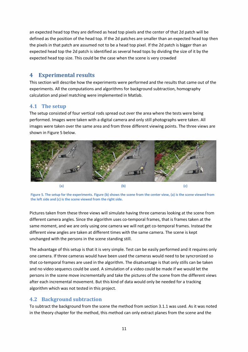
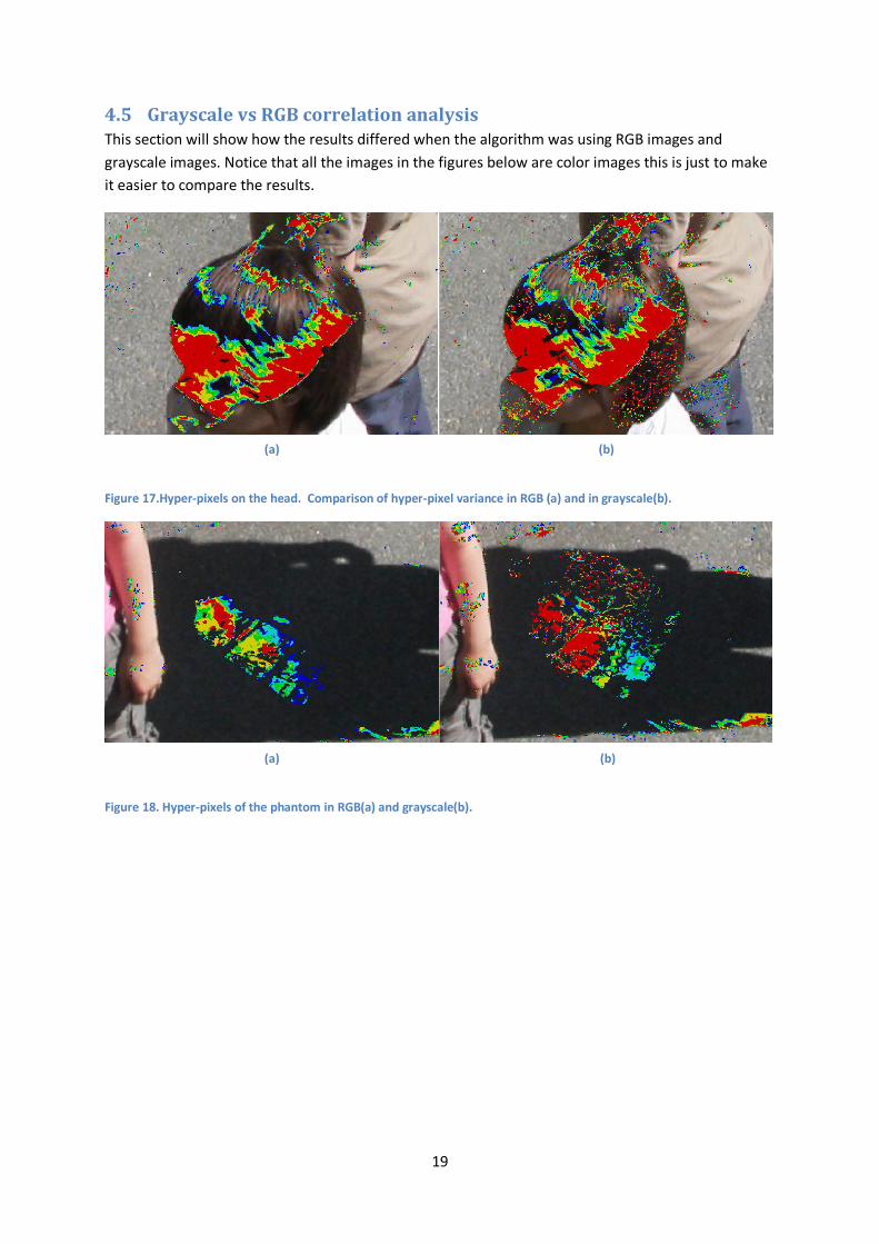
4.5 Grayscale vs RGB correlation analysis This section will show how the results differed when the algorithm was using RGB images and
grayscale images. Notice that all the images in the figures below are color images this is just to make
it easier to compare the results.
Figure 17.Hyper-pixels on the head. Comparison of hyper-pixel variance in RGB (a) and in grayscale(b).
Figure 18. Hyper-pixels of the phantom in RGB(a) and grayscale(b).
(a) (b)
(a) (b)

20
Figure 19. Subtracted background using RGB images(a) and grayscale images(b).
To analyze the performance of the method using RGB images against grayscale images the method
using RGB images was first tuned to give the best possible result it could get without getting to many
false positive detections. The method using grayscale was then tuned to give the same amount of
true positive detections to see the difference in the false positive detections.
In Figure 17 we see that there is not much of a difference for the hyper pixels of the head top. But in
Figure 18 we see that the patch of the phantom is bigger and that the hyper-pixels of it are more
highly correlated when only grayscale images are used. Figure 19 shows the background subtraction
and here we see an obvious difference between the two images where a lot of the head is subtracted
by the grayscale method.
4.6 Discussion In this section we will discuss some observations that were made during the experiments. The two
main things that were tested were the background subtractor and RGB-image analysis. The RGB-
image analysis behaved as expected so most of the discussion will be focused on the background
subtractor.
The background subtraction method was especially applicable to this detection algorithm since it is
using the existing multiple camera setup. But the possibility in applying it in other systems needs to
be investigated. The background subtraction method was tested on a scene where only about 50
percent of the background was subtracted however the remaining 50 percent of the background had
such characteristics that the head top detection was not disturbed by it. Future work on the
background subtraction method would be investigating if it can be combined with some other
background subtractor to completely remove the background. The behavior of the algorithm is also
controlled by the way to determine the correlation of pixels and the threshold parameter. Future
work may include testing different correlation functions to see if a better result can be achieved. This
includes also the head detection algorithm.
To increase the amount of background subtracted in the scene the cameras can be installed so that
more of the ground plane is covered and less of other parts of the background are captured by the
camera. This can be achieved by aiming the cameras with a higher angle against the ground, maybe
even 90 degrees. Also if the cameras are aimed straight down towards the ground there will be other
possibilities to find the needed homographies. The method for finding the homographies are quite
(a) (b)

21
tedious since it needs some form of feature points in the scene. The next step would be trying to find
a method which could find the homographies without using feature point detection.
It was noticed that reflections on the hair, may cause some problems for the head top detection. The
background extractor may also encounter some problems if the ground is reflective, which is quite
usual for indoor scenes.
When analyzing the images in RGB instead of grayscale the results were better but the calculation
time increased since RGB images has three intensity values and grayscale only has one intensity
value. The longer calculation time may cause the algorithm to miss deadlines in a real-time system,
which needs to investigated.
5 Conclusion An already studied but quite new method for detecting and tracking people was restudied. Only the
detection part was covered and a few modifications were applied. These were:
1. A different background subtraction method was tested.
2. The results from the background subtraction were tested on the detection algorithm.
3. The detection algorithm used RGB-images in the correlation analysis instead of grayscale
images.
How these changes affected the results and some future work have already been mentioned in the
discussion section above and it could be concluded that the changes did improve the results but at
the expense of calculation time. Future work would include designing the algorithm in such way that
it can meet the deadlines in a real time system. One big drawback of the method is the way
homographies are calculated, which is by extracting points from installed feature points I the scene.
No other method for doing this was presented in this thesis. However if a better method for doing
this can be found were no feature points are needed it would give the method much better
conditions to be applied in a practical context.

References
Keck, Davis & Tyagi (2006). Tracking Mean Shift Clustered Point Clouds for 3D Surveillance.
Proceeding VSSN '06 Proceedings of the 4th ACM international workshop on Video surveillance and
sensor networks (pp. 187-194)
Garibotto & Cibei (2005). 3D scene analysis by real-time stereovision. Image Processing, 2005. ICIP
2005. IEEE International Conference on. Volume 2. (pp. II - 105-8)
Kobayashi, Sugimura, Sato, Hirasawa, Suzuki, Kage & Sugimoto (2006). 3D head tracking using the
particle filter with cascaded classifiers. In Proceedings of the British machine vision conference
(BMVC) (pp. I-37).
Du & Piater (2007). Multi-camera people tracking by collaborative particle filters and principal axis-
based integration. In Proceedings of the Asian conference on computer vision (ACCV) (pp. 365-374).
Khan & Shah (2006). A Multiview Approach to Tracking People in Crowded Scenes Using a Planar
Homography Constraint. In Proceedings of the European conference on computer vision (ECCV) (pp.
IV: 133-146)
Eshel Moses (2010). Tracking in a Dense Crowd Using Multiple Cameras. International Journal of
Computer Vision. Volume 88, Number 1 (pp. 129-143)
Hartley & Zisserman (2003). Multiple View Geometry in Computer Vision. Second edition. (pp. 88-91)