Hauser (2006) logistic response model

8/7/2019 Hauser (2006) logistic response model

http://slidepdf.com/reader/full/hauser-2006-logistic-response-model 1/32

Another Look at the Stratification of Educational Transitions:

The Logistic Response Model with Partial

Proportionality Constraints*

Robert M. Hauser

Megan Andrew

Center for Demography of Health and AgingUniversity of Wisconsin-Madison

Rev. June 15, 2006

* Forthcoming in Sociological Methodology 2006 . An earlier version of this paper was prepared for the May 2005meetings of the Research Committee on Social Stratification, International Sociological Association in Oslo,

Norway. The research reported herein was supported by the William Vilas Estate Trust and by the Graduate Schoolof the University of Wisconsin-Madison. Computation was carried out using facilities of the Center for Demographyand Ecology at the University of Wisconsin-Madison, which are supported by Center Grants from the NationalInstitute of Child Health and Human Development and from the National Institute on Aging. We thank MaartenBuis, Jeremy Freese, Carl Frederick, Harry Ganzeboom, Michael Hout, and John A. Logan for helpful comments. ,We thank Robert D. Mare especially for correcting a serious error in an earlier draft of this paper and for his elegantand useful discussion of our work. The opinions expressed here are those of the authors. Address correspondence toRobert M. Hauser or Megan Andrew, Center for Demography and Ecology, University of Wisconsin-Madison, 1180Observatory Drive, Madison, Wisconsin 53706 or e-mail to [email protected] or [email protected].



1

ABSTRACT

In this paper we reanalyze Robert D. Mare’s highly influential analyses of educational

transitions among American men born in the first half of the 20 th century. Contrary to previous

belief, Mare found that the effects of socioeconomic background variables decline regularly

across educational transitions in conditional logistic regression analyses. We have reconfirmed

Mare’s findings and tested them by introducing a modified conditional logistic regression model

that constrains selected social background effects to vary proportionately across educational

transitions. We refer to our preferred model as the conditional logistic model with partial

proportionality constraints (CLPPC). The model can easily be estimated in Stata or using other

standard statistical software. Partial proportionality constraints may also prove useful in

interpopulation comparisons based on other linear models.



2

Robert Mare’s (1979; 1980; 1981) innovative analyses of American educational

transitions in the 1973 Occupational Changes in a Generation Survey (OCG) were among the

most important and influential contributions to research on social stratification in the past three

decades. Prior to the introduction of Mare’s model of educational transitions in 1980, social

stratification research typically employed linear probability models of school continuation and

linear models of highest grade completed, e.g., Hauser and Featherman (1976). This research

uniformly emphasized the stability of the stratification process in general and the effects of

parental socioeconomic status on educational attainment. In his analyses, Mare applied a logistic

response model to school continuation, restricting the base population at risk for each successive

transition to those who had completed the prior educational transition. Contrary to prior

supposition, Mare’s estimates suggested the effects of some socioeconomic background

variables declined across six successive transitions including completion of elementary school

through entry into graduate school.

Mare’s studies of educational transitions have been both influential and controversial.

His work spawned theories on the transition rates and odds ratios within educational systems,

most notably the theories of Maximally Maintained Inequality (Raftery and Hout 1993) and

Effectively Maintained Inequality (Lucas 2001). Mare’s models were also the basis of a widely

cited international comparative study of educational attainment (Shavit and Blossfeld 1993).

However, the thesis that effects of social background decline across educational transitions has

also been attacked by prominent labor economists (Cameron and Heckman 1998). They

suggested, among other things, that Mare’s logistic response model is only loosely behaviorally

motivated and that the general decline of social background effects is a statistical artifact of the

(logistic) parameterization of the model. However, Stolzenberg’s (1994) probit analysis



3

reconfirmed Mare’s finding that socioeconomic background has little or no influence on

transitions from college to graduate training in an American cohort that completed college in the

mid-1970s, and he explains the null finding by decay in the effects of SES on aspirations for

further schooling. Sociologists have also criticized Mare’s logistic response model of educational

transitions. Applying multinomial logit models to longitudinal data from Sweden, Breen and

Jonsson (2000) showed that class-origin effects on transition probabilities varied according to the

particular choice made at a given transition point and that the probability of making a particular

choice was path dependent.

Given the impact of Mare’s work and the continuing controversy surrounding logistic

response models of educational transitions, we return to the data originally analyzed by Mare in

an appreciative effort to validate and extend his model. We introduce a modified version of his

model that explicitly expresses and estimates changes in social origin effects across educational

transitions. Rather than analyzing each educational transition separately as Mare did, we

estimate a single model across all educational transitions. In this model, the relative effects of

some (but not all) background variables are the same at each transition, and multiplicative scalars

express proportional change in the effect of those variables across successive transitions.

Models of Educational Stratification: A Review

Aside from linear regression and linear probability models, researchers in educational

stratification have employed a number of more appropriate models to explore the effects of

social background on educational transitions, including logistic response, loglinear, and

multinomial models. Each model has advantages and disadvantages in the study of educational

transitions. Logistic response or continuation odds models employ conditional samples across



4

successive educational transitions and allow for the estimation of robust coefficients that are

invariant to marginal changes in educational attainment. In these models, continuation

probabilities are asymptotically independent; a model may be estimated separately for each

transition, or multiple transitions may be analyzed within a single model (Bishop, Fienberg, and

Holland 1975; Fienberg 1977). While logistic response models have been widely used in

stratification research, these models require a large number of parameters, allowing effects of

covariates to fluctuate freely across transitions whether or not they vary in the population.

Erikson and Goldthorpe’s (1992: 91-92) model of uniform differences in parameters of

social mobility, Xie’s (1992) log-multiplicative layer model for comparing mobility tables, and

Hout, Brooks, and Manza’s (1995: 812) model of trends in class voting in the U.S. each resemble

the model introduced here by imposing proportionality constraints on the coefficients of a model

across multiple populations .1 These models provide population average estimates of changes in

an outcome over time or place, but they do not easily allow for the introduction of individual-

level covariates. Moreover, estimation problems may occur when log-linear models are

extended to higher dimensions or in instances where the analyst wishes to consider more than

three or four transitions, whether they be educational transitions or transitions among

occupational groups.

Multinomial models have also been used to study educational transitions, though perhaps

less often than logistic response and log-linear models. Multinomial models provide the

opportunity to assess horizontal stratification in tandem with vertical stratification, allowing for a

richer analysis in some instances (Breen and Jonsson 2000). Anderson’s (1984) well-known

stereotype regression model provides a flexible means to consider proportionality of the effect of

a group(s) of covariates on ordered outcomes but has been relatively ignored in educational

1 We thank Michael Hout for bringing these similarities to our attention.



5

stratification research. This model is an important analytic tool in many respects. For example,

DiPrete’s exemplary paper (1990) uses stereotype regression models to introduce individual-

level covariates in social mobility analyses. However, multinomial models are of limited value

in the analysis of educational transitions. They specify multiple and possibly ordered categorical

outcomes but do not model the conditional risk of transitions. With the exception of stereotype

regression models, multinomial models also include a large number of coefficients. As in the

case of unrestricted logistic response models, these may add unnecessary complexity and may

make it difficult to interpret findings.

Given the various weaknesses of existing models of educational transitions and in an

effort to extend statistical models of educational stratification, we propose a logistic response

model with partial proportionality constraints. We believe that the model proposed here provides

a parsimonious and powerful description of changes in the effects of socioeconomic background

on educational attainment and, equally important, that it has wide application in studies of

changes and differentials in social stratification.

Logistic Response Models with Partial Proportionality Constraints

We begin with a logistic response model in Mare’s (1980: 297) notation:

0log ( ) ,1

ije j jk ijk

ij k

pX

pβ β = +

−∑ (1)

where ijp is the probability that the ith person will complete the jth school transition, ijk X is the

value of the k th explanatory variable for the ith person who is at risk of the jth transition, and the

jk β are parameters to be estimated. That is, for each transition a logistic response model is

estimated for persons at risk of completing that transition with no constraints on any parameters

across transitions. Delineated above, the logistic response model has two important properties.



6

First, the effects in equation 1 are invariant to the marginal distribution of schooling outcomes.

That is, for k > 0, a given set of jk β is consistent with any rate of completion of a transition.

Second, the continuation probabilities are asymptotically independent of one another (Fienberg

1977). Thus, the model may be estimated separately for each transition, or multiple transitions

may be analyzed within a single model.

Suppose that instead of analyzing the data for each transition separately the data are

converted to person-transition records. Thus, a record appears for each transition for which each

individual is eligible. In each record, there is a single outcome variable, say, y ij, where yij = 1 if

the transition is completed and yij = 0 if it is not completed. Since the transitions are ordered and

each transition is conditional on completion of prior transitions, there is at most one record for

which yij = 0 for each individual, namely, for the last transition for which that individual is

eligible; at all prior transitions, yij =1. In this setup, for example, one could estimate a model that

is similar to equation 1, except there is only one set of regression parameters, which apply

equally to each transition:

0log ( ) .1

ije j k ijk

ij k

pX

pβ β = +

−∑ (2)

This model, like that of equation 1, may be estimated with any software that supports logistic

regression analysis.

However, the hypothesis that socioeconomic background effects decline across

transitions might suggest a different and more parsimonious model. We refer to this as the

logistic response model with proprortionality constraints (LRPC):

0log ( ) ,1

ije j j k ijk

ij k

pX

pβ λ β = +

−∑ (3)



7

The first term on the right-hand side of equation 3 says there may be a different intercept at each

transition. The summation represents effects of the ijk X that are invariant across all transitions;

notice there is no j index on k β . However, there is a multiplicative scalar for each transition, jλ ,

which rescales the k β at each transition, subject to the normalizing constraint that 1λ =1. That is,

the jλ introduce proportional increases or decreases in the k β across transitions; thus, equation 3

implies proportional changes in main effects across transitions. The proportionally constrained

covariate(s) determine a composite variable, which can be interpreted in reference to (a) latent

theoretical construct(s). In this instance, the main effects of the covariates can be interpreted as

the weights of these covariates in that composite. Although equation 3 may appear to have more

terms than equation 2, it is actually more parsimonious because there are only as many

interaction terms as transitions. Equation 2 has as many interaction terms as the product of the

number of explanatory variables and the number of transitions.

Conceptually, the model in equation 3 is similar to the well-known MIMIC (multiple

indicator, multiple cause) model of Hauser, Goldberger, and Jöreskog (Hauser and Goldberger

1971; Hauser 1973; Jöreskog and Goldberger 1975; Hauser and Goldberger 1975). However,

proportionality constraints appear within a single-equation model estimated simultaneously in

two or more populations whereas the MIMIC model imposes proportionality constraints across

the coefficients of two or more equations estimated within a single population.

Several readers have suggested that the model of equation 3 is the same as the stereotype

model, which imposes proportionality constraints on coefficients across response categories in a

multinomial logistic model; however, the stereotype model pertains to a single population and

does not account for the conditional risk of transitions from one category to the next. If there



8

were more than two potential outcomes at each transition, one could possibly combine features

of the stereotype and CLPC models.

Our argument is that one ought to estimate a model like that in equation 3 before

proposing more complex explanations of change in the effects of socioeconomic background

variables across educational transitions. However, one cannot simply jump from the finding that

the model of equation 3 fits a set of data to the conclusion that the effects of background

variables are the same across transitions up to a coefficient of proportionality. Allison (1999)

shows that, if the model of equation 3 fits a set of data, one cannot distinguish empirically

between the hypothesis of uniform proportionality of effects across transitions and the hypothesis

that group differences between parameters of binary regressions are artifacts of heterogeneity

between groups in residual variation.2

It is also possible to mix the features of equations 2 and 3 to permit some variables to

interact freely with a given transition while others follow a model of proportional change, that is,

a conditional logistic with partial proportionality constraints (CLPPC):

'

0

1 ' 1

log ( ) ,1

k K ij

e j j k ijk jk ijk

ij k k

pX X

pβ λ β β

= +

= + +−

∑ ∑ (4)

Equation 4 says that for some variables, k X , where k = 1, …, k ′ , there is proportional change in

effects across transitions, while for other k X , k = k ′ + 1, … K, the effects interact freely with

transition level. For example, equation 4 could apply to Mare’s analysis, where effects of

socioeconomic variables appear to decline across transitions, while those of farm origin, one-

parent family, and Southern birth vary in other ways.

2 Ballarino and Schadee (2005) advance this argument in the context of an analysis of educational transitions in Italyand several other nations.



9

Equation 4 may be generalized to cover multiple cohorts as well as multiple transitions.

For example, equation 5 is one such generalization:

' ''

0

1 ' 1 1 '' 1

log ( ) ,

1

k K k K ijt

e jt j k ijtk jk ijtk t k ijtk tk ijtk

ijt k k k k

pX X X X

p

β λ β β γ β β = + = +

= + + + +

−∑ ∑ ∑ ∑ (5)

Here, for one set of variables, effects change proportionately across transition levels, j; for

another (possibly overlapping) set of variables, effects change proportionately across time

periods, indexed by t . The effects of the remaining sets of variables may interact freely with

transition level j and with period t .

Estimation of equations 3 through 5 is not as simple as that of equations 1 and 2. The

same linear expression, such as k ijk

k

X β ∑ , appears twice in the former equations--once with freely

estimated coefficients and again as a linear composite in j k ijk

k

X λ β ∑ . The problem is to estimate

the models in a way that will yield the same estimates of the k β in both expressions. One way to

accomplish this is simply to iterate. First, estimate the k β in a model with no interactions. Then,

estimate the model again with an interaction in the composite estimated in the previous step, and

continue until the fit and parameter values change very little from one iteration to the next

(Allison 1999; MacLean 2004). We have used another method, writing the equations of the

models and estimating them directly by maximum likelihood in Stata (see Appendix).3 It may

also be possible to estimate this model as if it were a MIMIC model (with uncorrelated outcome

variables) using MPlus or other software for estimation of structural equation models.

In summary, this framework allows for the estimation of parsimonious, single equation

models of educational transitions and addresses many of the shortcomings in extant models of

3 We thank Jeremy Freese for writing a macro in Stata 9 to estimate the model by maximum likelihood. For similarspecifications in Stata and other statistical packages, see Allison (1999).



10

educational transitions. These models are invariant to change in the marginal distribution, but

they use fewer parameters and are characterized by ease in the introduction of individual-level

covariates. These models can include uniform and/or partial proportionality constraints across

model covariates and transitions of interest while freely estimating effects of other model

covariates. Moreover, proportionality constraints in these models can be interpreted as indicative

of a latent construct similar to that in the MIMIC model. Yet another possibility is to constrain

the effects of a subset of variables to be invariant across populations. Finally, these models of

educational transitions easily allow for nuanced and powerful tests of the significance of

estimated differences in the effects of model covariates across educational transitions and, thus,

more informative inferences about the effects of social background on educational transitions.

We next apply this framework in a replication of Mare’s (1980, 1981) original work on

educational transitions.

Replicating and Extending Logistic Response Models Using the 1973 Occupational

Changes in a Generation Survey

In replicating Mare’s (1980) original analysis, we use the 1973 Occupational Changes in

a Generation (OCG) survey data, converting individual records to person-transition records. The

OCG survey was carried out as a supplement to the March 1973 Current Population Survey

(CPS). It was carried out via mail in September 1973 after all of the households participating in

the March demographic supplement had rotated out of the CPS. The response rate was 83

percent among target males. The present analysis includes 21,682 white men 21 to 65 years old

in the civilian noninstitutional population who responded to all of the social background

questions in the OCG supplement.



11

Father’s occupational status (FASEI) is the value of the Duncan Socioeconomic Index for

Occupations (Duncan 1961); scale values were assigned using an adaptation of the original scale

to codes for occupation, industry, and class of worker that were used in the Census of 1970.4

Number of siblings (SIBS) is based on questions about the number of older and younger siblings

of each sex. The count of siblings was top-coded at 9. Family income (FAMINC) was

represented by categorical responses to the question, “When you were about 16 years old, what

was your family’s annual income.” Pretest respondents indicated that they answered in

contemporary rather than price-adjusted dollars, so we adjusted the midpoints of responses from

dollars in the year that the participant turned 16 to 1967 dollars using the Consumer Price Index.

We assigned reports of “no income or loss” to the lowest reporting category ($1-499). After

examining scatterplots of the relationship between various transformations of income and the

probabilities of educational transitions, we top-coded the adjusted incomes at 2.5 standard

deviations above the mean and re-expressed the variable in natural logs. Father’s education

(FED) and mother’s education (MED) are expressed in years of regular schooling completed.

Participants were coded as living in a broken family (BROKEN) if they responded, “no,” to the

question, “Were you living with both your parents most of the time up to age 16?” A dummy

variable for farm origin (FARM) was coded 1 if the participant said that he had not moved since

age 16 (in the OCG survey) and currently lived on a farm (as reported in the CPS) or if he

reported in the OCG survey that he had lived on a farm when he was 16 years old; otherwise,

FARM was coded 0. State of birth was ascertained in the OCG survey, and a dummy variable

(SOUTH) was created for men born in a Southern state as defined by the U.S. Bureau of the

Census. With the exception of family income, all of the continuous background variables have

4 Our code for the Duncan SEI differs from that used by Mare. This code is more fine-grained than that which wasavailable to Mare (1980, 1981) though the results are largely the same.





13

Replicating Traditional Logistic Response Models

Table 4 reports our unconstrained estimates of the effects of social background variables

on educational transitions in the 1973 OCG data. These estimates were based on equation 1 and

replicate Mare’s (1980) original logistic response model. The coefficients differ from those

estimated by Mare (1980) for several reasons. Either we did not use the same version of the

1973 OCG data file or our sample definition was different from Mare’s in some way that we

have been unable to determine. We use a different scheme for scaling father’s occupational

status and a logarithmic transformation of family income. Moreover, we used all of the available

cases at every transition and defined the base population for college graduation to include those

who attended college, but did not complete at least one year of college.

Despite these differences in variable definitions and case selection, the estimates in Table

4 follow the main patterns of Mare’s estimates (Table 1). Social background explains less of the

variation at each higher educational transition, and the effects of the socioeconomic background

variables as defined by Mare (FASEI, FAMINC, FED, MED, and SIBS) typically decline from

lower to higher educational transitions. Similarly, effects of the other background variables

(BROKEN, FARM, and SOUTH) do not show the same pattern of decline across transitions.

Extending Traditional Logistic Response Models: The Logistic Response Model with Partial

Proportionality Constraints

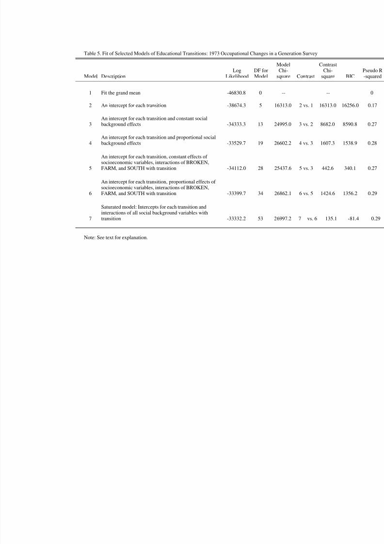
Table 5 describes the fit of models estimated for the combination of all six educational

transitions. Model 1 is a null baseline in which no parameters are fitted except the grand mean.



14

The likelihood ratio test statistic under this model defines the denominator of the pseudo-R2

statistics and can be used to measure improvements in the fit of more complex models. Model 2

fits an intercept for each transition, and it yields a substantial improvement in fit. Model 3 adds

invariant effects of social background variables to Model 2. This follows the scheme of equation

2. Overall rates of transition vary across levels of schooling, but the effects of social background

do not vary across transitions. This modification also yields a substantial improvement in fit.

Model 4 is based on equation 3. Rather than specifying constant effects of the eight

social background variables, it says that the all of the background effects vary in the same

proportion across each transition. With six more degrees of freedom, the parameters of

proportional change yield an improved model fit (change in the chi-square statistic of 1607.3).

Evidently, substantial variation in effects of background across educational transitions is

captured by the model of proportional change. However, Model 4 does not fit the data well.

Model 7 fits all of the interactions between social background variables and transitions, and its fit

is significantly better than that of Model 4 (chi-square of 395 with 34 degrees of freedom).

Moreover, as noted above, the improvement of fit in Model 4 relative to Model 3 does not tell us

whether the background effects actually vary proportionately across transitions or whether there

are corresponding differences in residual variation across transitions.

Model 5 specifies constant effects of the socioeconomic background variables (FASEI,

FAMINC, MED, and FED) and number of siblings (SIBS), but it permits effects of the other

three background variables (BROKEN, FARM, and SOUTH) to interact freely with transition

level. Note that Model 5 is a special case of equation 2 – because some effects do not vary

across educational transitions – and that Model 4 is not nested within Model 5. Comparing



15

Model 5 to Model 3, we find a significant improvement in fit, but it is only about a quarter of the

improvement from Model 3 to Model 4 and uses 15 degrees of freedom.

Model 6 is based on the specification of Model 5, but it adds proportional change across

transitions in the effects of FASEI, FAMINC, MED, FED, and SIBS. It is an example of the

model specified in equation 4. The improvement of fit in Model 6 relative to Model 5 is almost

as large as in that of Model 4 relative to Model 3. That is, even after the introduction of freely

estimated interaction effects between each transition level and BROKEN, FARM, and SOUTH,

fit is improved substantially by the specification of proportional change in effects of

socioeconomic background across educational transitions. However, because proportionality

constraints apply only to a subset of the background effects in Model 6, we know that variation

in coefficients across equations is not entirely due to residual variation in transitions.

Finally, Model 7 is an example of the specification in equation 2 in which effects of all

background variables are permitted to interact with educational transition levels. Although it

uses 19 more parameters than Model 6, the improvement in fit is negligible by comparison with

the other contrasts in Table 5. Thus, we prefer Model 6 to Model 7 and the other models listed in

Table 5. This decision is confirmed by the BIC statistics for contrasts between models, which

are also reported in Table 5. Excepting the contrast between Models 6 and 7, there is a

substantial improvement in BIC between each successive model.

Table 6 shows the estimated parameters of Model 6. Recall that this model includes

additive effects of all of the social background variables, freely estimated interactions of broken

family, farm background, and Southern birth with transition level, and multiplicative effects of

transition level with a linear composite of the socioeconomic variables and number of siblings.



16

Table 6 identifies four groups of parameters: (a) freely estimated additive effects, (b)

freely estimated interaction effects, (c) multiplicative effects, and (d) additive effects and

multiplicative composite. However, the first two groups are not distinct for purposes of

estimation. In this instance, group (a) includes the main effects of each transition level and the

main effects of broken family, farm background, and Southern birth while group (b) comprises

the interaction effects of broken family, farm background, and Southern birth with each

educational transition. There are no interaction effects with the first transition because the main

effects of broken family, farm background, and Southern birth are defined to reference that

transition. Group (c) specifies the multiplicative effects of the second through sixth transitions

relative to the effects of socioeconomic background in the first transition. Finally, group (d)

includes the main effects of the socioeconomic variables and number of siblings, which are also

the weights of those variables in the composite that interacts with educational transition level.

The estimates of direct interest in Table 6 are the main effects of the socioeconomic

variables (d) and the multiplicative effects of the transition levels (c). As one should expect, the

main effects of father’s occupational status, family income, mother’s education, and father’s

education are positive and highly significant, while that of number of siblings is negative and

highly significant. The multiplicative effects of transition level are also highly significant, and

they are increasingly negative at higher level transitions. These coefficients may appear

anomalous at first sight, but increasingly negative effects are exactly what we should expect.

That is, at each higher transition level, there is a larger proportional decrement in the main

effects of the socioeconomic variables. For example, the estimate of -.2257 for the transition to

high school conditional upon completion of elementary school says that the total effect of each

socioeconomic background variable is 20.3 percent smaller at the transition from elementary



17

school to high school than it is at the transition from school entry to the completion of

elementary school. Note that the decrements in the multiplicative effects are not equal across

transitions. The largest decrement is that between college entry and college completion (-0.7804

– (-0.4312) = -0.3492), and the second largest is between elementary school completion and high

school entry (-0.2257).

To illustrate the implications of these estimates for the total effects of each of the social

background variables, we insert the parameter estimates into the linear model (equation 4) and

rearrange terms. The first panel of Table 7 displays the total effects in Model 6 that are implied

by the parameter estimates. As expected, the effects of father’s occupational status, number of

siblings, family income, and parents’ educations decline regularly across transitions, while those

of broken family, farm background, and Southern birth do not. In the second panel, for purposes

of comparison, we show the corresponding unconstrained estimates from Model 7.7 The latter

are necessarily identical to those in Table 4 because Model 7 fits all of the background by level

interactions. The third panel shows the deviations of the estimates in Model 6 from those in

Model 7.

As we should expect from the contrast reported in Table 5 between Models 6 and 7, the

deviations in the third panel are small in most cases. The largest single deviation (-0.199)

pertains to the anomalously large and negative effect of family income on the transition from

college to graduate school. A second large deviation is an under-prediction of the salutary effect

of farm background on the completion of college. One notable pattern in the deviations is that

the model underestimates the effect of father’s occupational status on higher-level transitions,

7 We are concerned here mainly with the deviations in the effects of social background variables, and not with theintercepts.



18

and it overestimates the effects of the other background variables in the linear composite at those

levels.8

Conceivably, one might argue that father’s occupational status should be removed from

the linear composite in the other social background variables and interacted freely with transition

levels. However, such a decision – along with the inclusion of number of siblings in the linear

composite – would be inconsistent with the more general finding that socioeconomic effects vary

proportionately across transition levels. We should then be left with a less parsimonious and less

appealing claim that some socioeconomic effects vary proportionately while others do not. In

addition, because there is only one discrepant effect, we think that the evidence of non-

proportionality is weak, and we have not modified the model.

Discussion

In this analysis, we have shown that specification of interaction effects with a linear

composite is a parsimonious way to represent and assess the way in which social background

effects vary across educational transitions. In the case of Robert Mare’s analysis of educational

transitions among American men, we have shown that this model reproduces most of the

empirical features of his estimates. While estimation of the model is not as straightforward as an

ordinary regression analysis, it can be done easily and quickly with standard statistical software.

We can think of several other ways in which models with interaction effects with a linear

composite could be useful. We have already noted earlier applications of a similar idea to

comparative analysis of mobility tables (Erikson and Goldthorpe 1992; Xie 1992) and to trends

in class voting (Hout et al. 1995). One obvious extension is to analyses, like those in Mare

8 This is consistent with Mare’s (1980: 302-3) observations about the pattern of coefficients in the unrestrictedestimates.



19

(1979) and in Persistent Inequality (Shavit and Blossfeld 1993) where multiple educational

transitions have been observed in several cohorts.9

Such models, we believe, would also be

useful to structure and discipline international comparative analyses, such as pooled analyses of

the data used in Persistent Inequality or other cross-national studies that have been designed

specifically to create comparable data. We hope that similar models and methods may prove

useful across a wide range of research questions in the social and behavioral sciences.

9 Equation 5 of this paper provides a template for such analyses.



20

Reference List

Allison, Paul D. 1999. "Comparing Logit and Probit Coefficients Across Groups." Sociological

Methods Research 28(2):186-208.

Anderson, J. A. 1984. "Regression and Ordered Categorical Variables." Journal of the Royal

Statistical Society. Series B (Methodological) 46(1):1-30.

Ballarino, Gabriele and Hans Schadee. 2005. "Really Persisting Inequalities?"Research

Committee on Social Stratification, International Sociological Association. University of

California, Los Angeles.

Bishop, Yvonne M. M., Stephen E. Fienberg, and Paul W. Holland. 1975. Discrete Multivariate

Analysis: Theory and Practice. Cambridge, Mass.: MIT Press.

Breen, Richard and Jan O. Jonsson. 2000. "Analyzing Educational Careers: A Multinomial

Transition Model." American Sociological Review 65(5):754-72.

Cameron, Stephen V. and James J. Heckman. 1998. "Life Cycle Schooling and Dynamic

Selection Bias: Models and Evidence for Five Cohorts of American Males." Journal of

Political Economy 106(2):262-333.

DiPrete, Thomas A. 1990. "Adding Covariates to Loglinear Models for the Study of Social

Mobility." American Sociological Review 55(5):757-73.



21

Duncan, Otis D. 1961. "A Socioeconomic Index for All Occupations." Pp. 109-38 in

Occupations and Social Status. edited by Albert J. Jr. Reiss. New York: Free Press.

Erikson, Robert and John H. Goldthorpe. 1992. The Constant Flux: A Study of Class Mobility in

Industrial Societies. Oxford: The Clarendon Press.

Fienberg, Stephen E. 1977. The Analysis of Cross-Classified Categorical Data: Theory and

Practice. Cambridge, Massachusetts: MIT Press.

Hauser, Robert M. 1973. "Disaggregating a Social-Psychological Model of Educational

Attainment." Pp. 255-84 in Structural Equation Models in the Social Sciences. edited by

A. S. Goldberger and O. D. Duncan. New York: Seminar Press.

Hauser, Robert M. 1997. "Indicators of High School Completion and Dropout." Pp. 152-84 in

Indicators of Children's Well-Being, edited by Robert M. Hauser, Brett V. Brown, and

William R. Prosser. New York: Russell Sage Foundation.

Hauser, Robert M. and David L. Featherman. 1976. "Equality of Schooling: Trends and

Prospects." Sociology of Education 49(2):99-120.

Hauser, Robert M. and Arthur S. Goldberger. 1971. "The Treatment of Unobservable Variables

in Path Analysis." Pp. 81-117 in Sociological Methodology 1971, edited by Herbert L.

Costner. San Francisco: Jossey-Bass.



22

Hauser, Robert M. and Arthur S. Goldberger. 1975. "Correction of 'The Treatment of

Unobservable Variables in Path Analysis'." Pp. 212-13 in Sociological Methodology

1975. edited by David R. Heise. San Francisco: Jossey-Bass.

Hout, Michael, Clem Brooks, and Jeff Manza. 1995. "The Democratic Class Struggle in the

United States, 1948-1992." American Sociological Review 60(6):805-28.

Jöreskog, Karl G. and Arthur S. Goldberger. 1975. "Estimation of a Model With Multiple

Indicators and Multiple Causes of a Single Latent Variable." Journal of the American

Statistical Association 70:631-39.

Lucas, Samuel R. 2001. "Effectively Maintained Inequality: Education Transitions, Track

Mobility, and Social Background Effects." American Journal of Sociology 106(6):1642-

90.

MacLean, Alair. 2004. "The Varieties of Veteran Experience: Cold War Military Service and the

Life Course." doctoral diss., Department of Sociology, University of Wisconsin,

Madison, Wisconsin.

Mare, Robert D. 1979. "Social Background Composition and Educational Growth." Demography

16(1):55-71.

. 1980. "Social Background and School Continuation Decisions." Journal of the

American Statistical Association 75:293-305.



23

. 1981. "Change and Stability in Educational Stratification." American Sociological

Review 46(1):72-87.

Raftery, Adrian E. and Michael Hout. 1993. "Maximally Maintained Inequality: Expansion,

Reform, and Opportunity in Irish Education, 1921-75." Sociology of Education 66(1):41-

62.

Shavit, Yossi and Hans-Peter Blossfeld. 1993. Persistent Inequality : Changing Educational

Attainment in Thirteen Countries. Boulder, Colo. : Westview Press.

Stolzenberg, Ross M. 1994. "Educational Continuation by College Graduates." American

Journal of Sociology 99(4):1042-77.

Xie, Yu. 1992. "The Log-Multiplicative Layer Effect Model for Comparing Mobility Tables."

American Sociological Review 57(3):380-395.



Table 1. Coefficients Representing Effects of Social Background Factors on School Continuation Decisions (from Mare (

Completes Attends High Completes High Attends College Co

Elementary School Given School Given Given Completes Colle

(0-8) Completes Attends High High School Atten

Elementary (8-9) School (9-12) (12-13) (1

Variable b b/se(b) b b/se(b) b b/se(b) b b/se(b) b

Intercept 0.9886 4.22 1.2410 5.40 -0.1778 -1.48 -1.7440 -15.98 -0.643

FASEI 0.0075 1.42 0.0041 0.87 0.0154 7.82 0.0145 10.49 0.011

SIBS -0.1325 -5.67 -0.1444 -6.40 -0.1335 -11.39 -0.1067 -9.53 -0.073

FAMINC 0.1067 5.36 0.0587 3.79 0.0655 8.57 0.0444 9.24 0.009

FED 0.1188 4.79 0.0939 3.96 0.0784 6.77 0.0420 4.47 0.007

MED 0.1677 7.16 0.1243 5.56 0.0815 7.11 0.0940 9.29 0.036

BROKEN -0.3163 -1.71 -0.1256 -0.64 -0.2192 -2.30 -0.0078 -0.09 -0.156

FARM -0.6060 -4.54 -1.0560 -7.94 0.3013 3.88 0.0107 0.14 0.113SOUTH -0.5948 -4.70 0.4182 3.03 -0.0973 -1.45 0.0309 0.53 -0.060

"R2" 0.270 0.178 0.120 0.091

x2(8) 770.4 497.2 1226.4 1332.2

N 5,368 5,009 9,301 7,732

Subsample % 25 25 50 50

NOTE : Dependent variables are the log odds of continuing from one schooling level to the next. Estimates are based on civilian noninstitutional population born 1907-1951 . Independent variables are FASEI: father's occupational Duncan socwas 16; SIBS: number of siblings; FAMINC: annual income of family in thousands of constant (1967) dollars when respo

of school completed; MED: mother's grades of school completed; BROKEN: absence of one or both parents from responage 16; FARM: respondent lived on a farm at age 16; SOUTH: respondent born in the South census region. x2 tests nulzero.



Table 2. Means and Standard Deviations of Social Background Variables at Selected Levels of SchooOccupational Changes in a Generation Survey

Level of Schooling

Father'sOccupation

(FASEI)

FamilyIncome

(FAMINC)

Father'sSchooling

(FED)

Mother'sschooling(MED)

Number ofSiblings(SIBS)

School Entry 31.4 1.773 8.6 9.1 3.7

22.9 0.900 4.1 3.8 2.6

Elementary School 32.6 1.857 9.0 9.5 3.5

Completion 23.1 0.832 3.9 3.6 2.5

High School 33.7 1.906 9.2 9.7 3.4

Attendance 23.3 0.800 3.9 3.5 2.5

High School 36.0 1.987 9.7 10.1 3.1

Graduation 23.8 0.764 3.8 3.4 2.4

College Attendance 42.8 2.165 10.7 11.0 2.6

25.1 0.710 3.9 3.3 2.1

College Graduation 46.6 2.226 11.1 11.3 2.4

25.3 0.698 3.9 3.3 2.0





Table 4. Coefficients Representing Effects of Social Background Factors on School Continuation: 1973 Occupational Ch

Completes Attends High Completes High Attends College Co

Elementary School Given School Given Given Completes Colle

(0-8) Completes Attends High High School Atten

Elementary (8-9) School (9-12) (12-13) (1

Variable b b/se(b) b b/se(b) b b/se(b) b b/se(b) b

Intercept 0.4655 4.45 0.8376 7.32 -0.1509 -1.78 -1.8544 -22.45 -0.435

FASEI 0.1731 6.87 0.2308 9.40 0.1575 11.98 0.1650 17.56 0.116

SIBS -0.1234 -10.83 -0.1397 -12.05 -0.1260 -15.21 -0.1042 -13.24 -0.088

FAMINC 0.5690 18.29 0.4013 11.87 0.2953 10.92 0.2976 11.04 0.021

FED 0.1216 10.13 0.0627 5.22 0.0566 7.10 0.0465 7.12 -0.011

MED 0.1496 13.15 0.1083 9.34 0.0911 11.46 0.0748 10.66 0.022

BROKEN -0.3121 -3.66 -0.0554 -0.57 -0.2228 -3.38 -0.1001 -1.64 -0.147FARM -0.1413 -2.08 -0.6979 -10.37 0.2811 4.80 -0.0278 -0.52 0.230

SOUTH -0.6419 -10.57 0.3268 4.71 -0.0771 -1.63 0.0131 0.31 -0.028

"R2" 0.313 0.191 0.134 0.120

x2(8) 3611.6 1868.4 2263.9 2582.1

N 21,682 20,058 18,725 15,602

NOTE : Dependent variables are the log odds of continuing from one schooling level to the next. Estimates are based on civilian noninstitutional population born 1907-1951. Independent variables are FASEI: father's occupational Duncan sociwas 16; SIBS: number of siblings; FAMINC: natural log of truncated annual income of family in thousands of constant (1

was 16; FED: father's grades of school completed; MED: mother's grades of school completed; BROKEN: absence of onehousehold most of the time to age 16; FARM: respondent lived on a farm at age 16; SOUTH: respondent born in the Southypothesis that all coefficients are zero.



Table 5. Fit of Selected Models of Educational Transitions: 1973 Occupational Changes in a Generation Survey

Model DescriptionLog

LikelihoodDF forModel

ModelChi-

square Contrast

C

1 Fit the grand mean -46830.8 0 --

2 An intercept for each transition -38674.3 5 16313.0 2 vs. 1 1

3An intercept for each transition and constant socialbackground effects -34333.3 13 24995.0 3 vs. 2 8

4An intercept for each transition and proportional socialbackground effects -33529.7 19 26602.2 4 vs. 3 1

5

An intercept for each transition, constant effects of socioeconomic variables, interactions of BROKEN,FARM, and SOUTH with transition -34112.0 28 25437.6 5 vs. 3

6

An intercept for each transition, proportional effects of socioeconomic variables, interactions of BROKEN,FARM, and SOUTH with transition -33399.7 34 26862.1 6 vs. 5 1

7

Saturated model: Intercepts for each transition andinteractions of all social background variables with

transition -33332.2 53 26997.2 7 vs. 6

Note: See text for explanation.



Table 6. Estimated Parameters of Model 6: 1973 Occupational Changes in a Generation Survey

Variable Coefficient Standard Error t-statistic

a. Freely estimated additive effects

Completes Elementary (0-8, TRANS1) 0.7815 0.0777 10.06

Attends High School If Completes Elementary (8-9, TRANS2) 0.7738 0.0655 11.82

Completes High School If Attends High School (9-12, TRANS3) -0.3125 0.0670 -4.66

Attends College If Completes High School (12-13, TRANS4) -1.9488 0.0613 -31.79

Completes College If Attends College (13-16, TRANS5) -0.9565 0.0734 -13.03

Attends Post-College If Completes College (16-17, TRANS6) -0.3145 0.1085 -2.90

Non-intact Family (BROKEN} -0.3453 0.0833 -4.15

Farm Background (FARM) -0.1010 0.0672 -1.50

Southern Birth (SOUTH) -0.6276 0.0612 -10.25

b. Freely estimated interaction effects

TRANS2 X BROKEN 0.2913 0.1265 2.30TRANS2 X FARM -0.6159 0.0929 -6.63

TRANS2 X SOUTH 0.9564 0.0914 10.47

TRANS3 X BROKEN 0.1390 0.1053 1.32

TRANS3 X FARM 0.3894 0.0885 4.40

TRANS3 X SOUTH 0.5488 0.0776 7.08

TRANS4 X BROKEN 0.2449 0.1024 2.39

TRANS4 X FARM 0.0506 0.0849 0.60

TRANS4 X SOUTH 0.6431 0.0740 8.69

TRANS5 X BROKEN 0.2326 0.1160 2.01

TRANS5 X FARM 0.2259 0.1018 2.22

TRANS5 X SOUTH 0.6058 0.0811 7.47

TRANS6 X BROKEN -0.0866 0.1473 -0.59

TRANS6 X FARM 0.0767 0.1303 0.59TRANS6 X SOUTH 0.3855 0.0967 3.99

c. Multiplicative Effects

Attends High School If Completes Elementary (8-9, TRANS2) -0.2257 0.0238 -9.50

Completes High School If Attends High School (9-12, TRANS3) -0.3704 0.0221 -16.76

Attends College If Completes High School (12-13, TRANS4) -0.4312 0.0180 -23.95

Completes College If Attends College (13-16, TRANS5) -0.7804 0.0157 -49.68

Attends Post-College If Completes College (16-17, TRANS6) -0.9159 0.0214 -42.73

d. Additive Effects and Multiplicative Composite

FASEI 0.2662 0.0123 21.55SIBS -0.1698 0.0072 -23.71

FAMINC 0.5233 0.0209 25.07

FED 0.0911 0.0066 13.90

MED 0.1435 0.0064 22.25

Note: See text for explanation.

27



Table 7. Comparison of Estimates from Preferred Model (6) with Estimates from Saturated Model (7)

Completes Attends High Completes High ttends College Completes Attends Post-

Elementary School Given School Given Given Completes College Given college Given

Variable (0-8) Completes Attends High High School Attends College Completes

Elementary (8-9) School (9-12) (12-13) (13-16) College (16-17)

Model 6: Intercept for each transition, proportional effects of socioeconomic variables, and interactions of BROKEN,FARM, and SOUTH with each transition

FASEI 0.266 0.206 0.168 0.151 0.058 0.022

SIBS -0.170 -0.132 -0.107 -0.097 -0.037 -0.014

FAMINC 0.523 0.405 0.329 0.298 0.115 0.044

FED 0.091 0.071 0.057 0.052 0.020 0.008

MED 0.143 0.111 0.090 0.082 0.032 0.012

BROKEN -0.345 -0.054 -0.206 -0.100 -0.113 -0.432

FARM -0.101 -0.717 0.288 -0.050 0.125 -0.024

SOUTH -0.628 0.329 -0.079 0.016 -0.022 -0.242

Intercept 0.781 0.774 -0.313 -1.949 -0.956 -0.314

Model 7: Saturated model with intercepts for each transition and interactions of all social background variables witheach transition

FASEI 0.173 0.231 0.158 0.165 0.116 0.068

SIBS -0.123 -0.140 -0.126 -0.104 -0.089 -0.005

FAMINC 0.569 0.401 0.295 0.298 0.021 -0.155

FED 0.122 0.063 0.057 0.047 -0.011 -0.007

MED 0.150 0.108 0.091 0.075 0.023 0.033

BROKEN -0.312 -0.055 -0.223 -0.100 -0.147 -0.501FARM -0.141 -0.698 0.281 -0.028 0.231 -0.015

SOUTH -0.642 0.327 -0.077 0.013 -0.029 -0.265

Intercept 0.465 0.838 -0.151 -1.854 -0.435 -0.163

Deviations (Model 7 - Model 6)

FASEI -0.093 0.025 -0.010 0.014 0.058 0.045

SIBS 0.046 -0.008 -0.019 -0.008 -0.052 0.010

FAMINC 0.046 -0.004 -0.034 -0.000 -0.094 -0.199

FED 0.030 -0.008 -0.001 -0.005 -0.031 -0.015

MED 0.006 -0.003 0.001 -0.007 -0.009 0.021BROKEN 0.033 -0.001 -0.016 0.000 -0.035 -0.069

FARM -0.040 0.019 -0.007 0.023 0.106 0.009

SOUTH -0.014 -0.002 0.002 -0.002 -0.007 -0.023

Intercept -0.316 0.064 0.162 0.094 0.521 0.152

28



APPENDIX

STATA CODE FOR PREFERRED MODEL

OF EDUCATIONAL TRANSITIONS

**Model 6: Continuous Parameters Constrained to Equality **

**Across Transitions, Discrete Parameters Vary Freely **

**Across Transitions**

capture program drop pclogit

program define pclogit

tempname theta

version 6

args lnf theta1 theta2 theta3

gen `theta' = `theta1' + `theta3' + (`theta2'*`theta3')

quietly replace `lnf' = ln(exp(`theta')/(1+exp(`theta'))) if

$ML_y1==1

quietly replace `lnf' = ln(1/(1+exp(`theta'))) if $ML_y1==0

end

ml model lf pclogit (outcome = trans1 trans2 trans3 trans4 trans5

trans6 broken farm16 south trans2Xbroken trans2Xfarm16 trans2Xsouth

trans3Xbroken trans3Xfarm16 trans3Xsouth trans4Xbroken trans4Xfarm16

trans4Xsouth trans5Xbroken trans5Xfarm16 trans5Xsouth trans6Xbroken

trans6Xfarm16 trans6Xsouth, nocons) (trans2 trans3 trans4 trans5 trans6,

nocons) (dunc sibsttl9 ln_inc_trunc edhifaom edhimoom, nocons)

**The following set of starting values are not essential **

**but estimation is much faster when starting values are assigned **

ml init eq1:trans1 =.4041526 eq1:trans2 =.7751678 eq1:trans3 =-

.3116492 eq1:trans4 =-1.948527 eq1:trans5 =-.9562174 eq1:trans6 =-.3119838

eq1:trans2Xbroken =-.0519577 eq1:trans2Xfarm16 =-.7136086 eq1:trans2Xsouth

=.3302017 eq1:trans3Xbroken = -.2044395 eq1:trans3Xfarm16 = .2908632

eq1:trans3Xsouth =-.0779455 eq1:trans4Xbroken =-.0985229 eq1:trans4Xfarm16 =-

.0484765 eq1:trans4Xsouth =.0161895 eq1:trans5Xbroken =-.1119574

eq1:trans5Xfarm16 =.1257399 eq1:trans5Xsouth = -.0215616 eq1:trans6Xbroken =-

.4318161 eq1:trans6Xfarm16 =-.0246239 eq1:trans6Xsouth =-.2418691 eq2:trans2 =-

.2524217 eq2:trans3 =-.3919983 eq2:trans4 =-.4505379 eq2:trans5 =-.7878735

eq2:trans6 =-.9192267 eq3:dunc =.2752204 eq3:sibsttl9 =-.1762127

eq3:ln_inc_trunc =.554373 eq3:edhifaom =.0953649 eq3:edhimoom =.1451568

ml maximize

Documents

Hauser (2006) logistic response model