Harrell 1996

STATISTICS IN MEDICINE, VOL. 15,361-387 (1996)

TUTORIAL IN BIOSTATISTICS

MULTIVARIABLE PROGNOSTIC MODELS: ISSUES IN DEVELOPING MODELS, EVALUATING

ASSUMPTIONS AND ADEQUACY, AND MEASURING AND REDUCING ERRORS

FRANK E. HARRELL Jr., KERRY L. LEE AND DANIEL B. MARK Divisions of Biometry and Cardiology. Box 3363. Duke University Medical Center, Durham. North Carolina 27710, U.S.A.

SUMMARY

Multivariable regression models are powerful tools that are used frequently in studies of clinical outcomes. These models can use a mixture of categorical and continuous variables and can handle partially observed (censored) responses. However, uncritical application of modelling techniques can result in models that poorly fit the dataset at hand, or, even more likely, inaccurately predict outcomes on new subjects. One must know how to measure qualities of a model's fit in order to avoid poorly fitted or overfitted models. Measurement of predictive accuracy can be difficult for survival time data in the presence of censoring. We discuss an easily interpretable index of predictive discrimination as well as methods for assessing calibration of predicted survival probabilities. Both types of predictive accuracy should be unbiasedly validated using bootstrapping or cross-validation, before using predictions in a new data series. We discuss some of the hazards of poorly fitted and overfitted regression models and present one modelling strategy that avoids many of the problems discussed. The methods described are applicable to all regression models, but are particularly needed for binary, ordinal, and time-to-event outcomes. Methods are illustrated with a survival analysis in prostate cancer using Cox regression.

1. INTRODUCTION

Accurate estimation of patient prognosis is important for many reasons. First, prognostic estimates can be used to inform the patient about likely outcomes of her disease. Second, the physician can use estimates of prognosis as a guide for ordering additional tests and selecting appropriate therapies. Third, prognostic assessments are useful in the evaluation of technologies; prognostic estimates derived both with and without using the results of a given test can be compared to measure the incremental prognostic information provided by that test over what is provided by prior information.' Fourth, a researcher may want to estimate the effect of a single factor (for example, treatment given) on prognosis in an observational study in which many uncontrolled confounding factors are also measured. Here the simultaneous effects of the uncontrolled variables must be controlled (held constant mathematically if using a regression model) so that the effect of the factor of interest can be more purely estimated. An analysis of how variables (especially continuous ones) affect the patient outcomes of interest is necessary to

CCC 0277-67 15/96/04036 1-27 0 1996 by John Wiley & Sons, Ltd.

362 F. HARRELL, K. LEE AND D. MARK

ascertain how to control their effects. Fifth, prognostic estimation is useful in designing randomized clinical trials. Both the decision concerning which patients to randomize and the design of the randomization process (for example, stratified randomization using prognostic factors) are aided by the availability of accurate prognostic estimates before randomization.* Lastly, accurate prognostic models can be used to test for differential therapeutic benefit or to estimate the clinical benefit for an individual patient in a clinical trial, taking into account the fact that low-risk patients must have less absolute benefit (lower change in survival pr~bability).~

To accomplish these objectives, analysts must create prognostic models that accurately reflect the patterns existing in the underlying data and that are valid when applied to comparable data in other settings or institutions. Models may be inaccurate due to violation of assumptions, omission of important predictors, high frequency of missing data and/or improper imputation methods, and especially with small datasets, overfitting. The purpose of this paper is to review methods for examining lack of fit and detection of overfitting of models and to suggest guidelines for maximizing model accuracy. Section 2 covers initial steps such as imputation of missing data, pre-specification of interactions, and choosing the outcome model. Section 3 has an overview of the need for data reduction. In Section 4, we discuss the process of checking whether a hypothesized model fits the data. In Section 5, measures of predictive accuracy are covered. These are not directly related to lack of fit but rather to the ability of the model to discriminate and be well calibrated when applied prospectively. Section 6 covers model validation and demonstrates advantages of resampling techniques. Section 7 provides one modelling strategy that takes into account ideas from earlier sections and lists some miscellaneous concerns. Most of the methods presented here can be used with any regression model. Section 8 briefly describes some statistical software useful in carrying out the strategy summarized in Section 7. Section 9 has a detailed case study using a Cox regression model for time until death in a clinical trial studying prostate cancer.

2. PRELIMINARY STEPS

Before analyses begin, the researcher must specify the relationships of interest and define and assemble the response variable and the potential predictors. At this point a frequent problem is the extent of missing data. Some methods of dealing with missing data are given in References 4-7. Deletion of cases with missing predictors causes bias and increased variance. Even though caution should be taken when imputing missing values, it is usually better to estimate selected data values than to delete an entire subject's record. Simple methods of imputation include the use of the median, mean, or mode for missing values. This method is biased and inefficient when predictors are correlated with one a n ~ t h e r . ~ Deriving customized regression models for predicting each predictor from all other predictors is a better method. Kuhfeld' has implemented a general imputation method that allows predictors to be non-linearly (and even non-monotoni- cally) related to one another. This method has been modified by Harrell and implemented in the S-Plus transcan function (Section 8), which yields stable imputations even when the fraction of missing values is quite large. In some cases, surrogate predictors, not intended to enter the model directly, are assembled to assist in imputing missing predictors in the model.

It is important that maximum information be extracted from predictors and response. Because of this and because of problems with data reliability, when one has a choice of describing a concept with a categorical variable or a continuous one, the continuous one is preferred. Subject matter knowledge should guide the selection of candidate predictors. Early deletion of those with little chance of being predictive or of being measured reliably will result in models with less overfitting and greater generalizability.

MULTIVARIABLE PROGNOSTIC MODELS 363

Plausible interactions should be carefully chosen because of problems of multiple parameters (see reference 9 for additional thoughts on interactions). Certain types of interactions that have frequently been found to be important in predicting clinical outcomes and thus may be pre- specified are:

1. Interactions between treatment and the severity of disease being treated. Patients with little disease have little opportunity to receive benefit.

2. Interactions involving age and risk factors. Old subjects are generally less affected by risk factors. They have been robust enough to survive to their current age with risk factors present.

3. Interactions involving age and type of disease. Some diseases are incurable and have the same prognosis regardless of age. Others are treatable or have less effect on younger patients.

4. Interactions between a measurement and the state of a subject during a measurement. For example, left ventricular function measured at rest may have less predictive value and thus have a smaller slope versus outcome than function measured during stress.

5. Interactions between calendar time and treatment. Some treatments evolve or their effectiveness improves with staff training.

6. Interactions between quality and quantity of a symptom.

Careful fitting of a statistical model is essential so that interactions, if present, represent biologic phenomena rather than general lack of fit of the model.

A tentative choice of the statistical model is sometimes based on previous distributional examinations, but it is frequently based on maximizing how available information is used. Binary and ordinal logistic models1c13 are frequently used for discrete completely assessed outcomes, and the Cox proportional hazards and parametric survival models16 are frequently used for censored time-to-event data. It is quite common to change the model after initial modelling of predictors, because only then can adjusted distributional properties of Y and joint properties of X and Y be assessed (Section 4.3).

3. DATA REDUCTION

Multivariable statistical models when developed carefully are excellent tools for making prognostic predictions. However, when the assumptions of a model are grossly violated or when a model is used unwisely for a given patient sample, the performance of the model may be poor. For example, when the analyst has fitted not only real trends that further data would support, but in addition has fitted idiosyncrasies in the particular dataset by analysing too many variables, the model may predict inaccurately for a new group of patients. Only with appropriate model validation can an apparently accurate model be shown to be inaccurate.

In developing a set of predictions based on 100 patients, no analyst would divide the patients into 50 subgroups and quote the average outcome for each subgroup. Yet many articles have appeared in the clinical literature where 20-50 variables were analysed on 100 patients. Re- searchers apparently do not realize that when many predictor variables are analysed, variable screening based on statistical significance and stepwise variable selection involve multiple comparisons problems that lead to unreliable models. These methods are therefore not viable for data reduction (see Reference 17 for a condemnation of stepwise variable selection).

The situation is actually worse than merely considering the number of predictors. If the analyst used associations with Y to entertain non-linearities in the predictors or interaction terms, these constructed variables need to be counted (see Table 11 for an example). We speak of the total


predictor degrees of freedom (d.f.), p, as the total number of parameters (columns of the design matrix) examined during the course of analysis, excluding intercept term(s). If graphical or other informal analyses are used to guide the analysis, it is difficult to define p - one needs to estimate the effective number of parameters considered according to the flexibility of fits that were considered.” The quantity p is the effective number of parameters allowed for consideration, that is, the number of regression coefficients estimated formally or informally without algebraic restrictions.

To enhance the accuracy of a model, the number of variables used must be reduced or the model must be simplified unless the sample is large. Unless a formal penalized estimation technique is used,lg multiple comparisons problems that arise from ‘peeking’ at the outcome variable must be eliminated; data reduction methods must be used that do not utilize the outcome variable. Harrell et ~ 1 . ~ ~ discussed some available data reduction methods and two regression modelling strategies based on these methods that yield reliable models. They suggest as a rough rule of thumb that in order to have predictive discrimination that validates on a new sample, no more than m/10 predictor d.f. p should be examined to fit a multiple regression model, where m is the number of uncensored event times (for example, deaths) in the training sample (the sample used in fitting the model). For binary outcomes m is the number of patients in the less frequent outcome category. If p > m/lO, a data reduction technique such as principal components, variable clustering, or deriving clinical summary should be used until the number of summary variables to use as candidates in the regression analysis is less than m/10.

Smith et ~ 1 . ’ ~ found in one series of simulations that the expected error* in Cox model predicted 5-year survival probabilities was below 0.05 when p < m/20 for ‘average’ subjects and below 0.10 when p < m/20 for ‘sick‘ subjects. For ‘average’ subjects, m/10 was adequate for preventing expected errors > 0.1.

Better and more general than any of these rules is the reduction of d.f. using a shrinkage method (Section 5.4).

4. VERIFYING MODEL ASSUMPTIONS: CHECKING LACK OF FIT

4.1. Linearity assumption

In their simplest forms, all usual regression models assume that for a certain scale of Y, each predictor variable X is linearly related to Y. In the logistic regression model for binary responses, the initial assumption is that an X is linearly related to the log odds of response (log[P/(l - P)], where P is the probability of response) for patients subgrouped by values of X. In the Cox proportional hazards survival model, one initially assumes that at each time t, log[ - log(S(t))] and equivalently logI(t) are linearly related to X, where S ( t ) is the probability of surviving until time t and I ( t ) is the hazard function or instantaneous event rate at time t. It is easy to envision cases where strong violations in the linearity assumption (say a U-shaped age relationship) will result in erroneous predictions.

A direct way to check the linearity assumption, and to determine how to transform a specific X if necessary, involves expanding X into multiple terms that can flexibly fit any smooth relationship. The extra terms can be statistically tested to assess the adequacy of a linear relationship, and the terms in toto can estimate the true transformation of X that would result in

* Absolute difference between predicted and actual 5-year survival probabilities in a simulation study with known survival functions


a linear relationship with Y. A common choice of expansion is to add X2 and perhaps higher powers of X to the model. A more flexible approach is the use of piecewise linear regression or piecewise cubic polynomials (spline functions). See references 25-27 for methods of fitting such functions.

As an alternative, smoothed residual plots can be used to determine the functional form for each predictor. For binary logistic models, smoothed partial residual are useful, and for the Cox model, smoothed martingale residuals plots detect regression shape departure^.^' Partial residuals in logistic models are particularly computationally efficient, as the analyst can fit a simple model that is linear in all predictors and then use the residuals to obtain estimates of the true functional forms. However, the plot for each predictor does assume that the other predictors operate linearly and that all predictors are additive (see below). The usual martingale residual plot for the Cox model provides an estimate of the departure from linearity for the predictor.

4.2. Additivity assumption

A further assumption of most regression models is additivity of effects of the predictors (lack of interaction). Interactions can be tested and described by adding cross-product terms. It must be borne in mind that interactions can take the form of a change in shape (for example, linear age relationship for males, quadratic for females), so the cross-products needed in the model are not always simple ones.

The number of possible cross-product terms is usually so large (especially when variables have nonlinear or multiple dummy variable components) that the predictors to check for additivity must usually be specified before examining the data. Otherwise, type I errors and overfitting will be significant problems. A compromise solution is to do pooled interaction tests. For example, in a model with predictors age, sex, and dose, one may test all second-order interactions involving age, all interactions involving sex, and all involving dose. A combined test of all two-way interactions is also useful. If a pooled test is not significant, it may be unwise to pursue significant component interactions.

4.3. Distributional assumption

The previous sections dealt with the proper specification of the X-structure of the model. Once the analyst has determined which predictors are to be used and how they should be represented in the model, most models have distributional assumptions that also need verification. The Cox model does not assume anything about the survival function S ( t ) across t for an individual, but it does assume how survival curves for different subjects are related. Specifically, it assumes that log[ - log(S(t))] for different subjects are equidistant over time, or equivalently that hazard functions for any two subjects are proportional over time. This proportional hazards assumption can be checked using smoothed plots of a special type of residual from the model called the Schoenfeld r e ~ i d u a l . ~ ' . ~ ~ It can also be checked using hazard ratio plots, plots of modelled versus stratified estimates,' and several other methods.33 Unlike the Cox model, fully parametric models (for example, Weibull or log-normal survival models) have a distributional assumption even when there are no covariables. If the form of S ( t ) does not fit the data for these models, estimates of S(t) will be inaccurate.

That is, a Cox model is fitted with the variable in question appearing as a covariate for which regression coeEcient(s) are estimated, then a second model is fitted where that variable is used as a stratification factor that modifies the underlying survival function (but which does not have regression coefficients).


5. QUANTIFYING PREDICTIVE ACCURACY

There are at least three uses of measures of predictive accuracy:

1. To quantify the utility of a predictor or model to be used for prediction or for screening to identify subjects at increased risk of a disease or clinical outcome.!

2. To check a given model for overfitting (fitting noise resulting in unstable regression coefficients) or lack of fit (improper model specification, omitted predictors, or underfitting). More will be said about this later.

3. To rank competing methods or competing models.

The measures discussed below may be applied to the assessment of a predictive model using the same sample on which the model was developed. However, this assessment is seldom of interest, as only the most serious lack of fit will make a model appear not to fit on the sample for which it was tailor-made. Of much greater value is the assessment of accuracy on a separate sample or a bias-corrected estimate of accuracy on the training sample. This assessment can detect gross lack of fit as well as overfitting, whereas the apparent accuracy from the original model development sample does not allow one to quantify overfitting. Section 6 discusses how the indexes described below may be estimated fairly using a validation technique.

5.1. General notions

In the simplest case, when the response being predicted is a continuous variable that is measured completely (as distinct from censored measurements caused by termination of follow-up before all subjects have had the outcome of interest), one commonly used measure of predictive accuracy is the expected squared error of the estimate. This quantity is defined as the expected squared difference between predicted and observed values, that is, the average squared difference between predicted and observed values if the experiment were repeated infinitely often and new estimates were made at each replication. The expected squared error can also be expressed as the square of the bias of the estimate plus the variance of the estimate. Here bias refers to the expected value of the estimate minus the quantity being estimated, such as the mean blood pressure. The expected squared error is estimated in practice by the usual mean squared error.

There are two other terms for describing the components of predictive accuracy: calibration and discrimination. Calibration refers to the extent of bias. For example, if the average predicted mortality for a group of similar patients is 0.3 and the actual proportion dying is 0.3, the predictions are well calibrated. Discrimination measures a predictor’s ability to separate patients with different responses. A weather forecaster who predicts a 015 chance of rain every day of the year may be well calibrated in a certain locality if the average number of days with rain is 55 per year, but the forecasts are uninformative. A discriminating forecaster would be one who assigns a wide distribution of predictions and whose predicted risks for days where rain actually occurred are larger than for dry days. If a predictive model has poor discrimination, no adjustment or

Often one wishes to designate a model as ‘minimally acceptable’ on the basis of some statistic, but in many cases it is only possible to judge a model’s accuracy relative to another model. For example, a model for the probability of death after open heart surgery may yield predicted probabilities that range from 0.001 to 0.1, so the model will not have a high correlation (say 0.13) between predicted probability and observed outcome, but it may still be useful. If that model does not fully adjust for patient risk factors, it may be inadequate for adjusting for case mix when comparing mortalities among several hospitals. A more sensitive model with a correlation of, say, 0,135 may adjust away apparent differences in mortality among hospitals.


calibration can correct the model. However, if discrimination is good, the predictor can be calibrated without sacrificing the discrimination (see Section 6 for a method for calibrating predictions without needing more data). Here, calibrating predictions means modifying them, without changing their rank order, such that the predictions are perfectly calibrated. van Houwelingen and le C e ~ s i e ~ ~ present extensive information on predictive accuracy and model validation.

5.2. Continuous uncensored outcomes

Discrimination is related to the expected squared error and to the correlation between predicted and observed responses. In the case of ordinary multiple linear regression, discrimination can be measured by the squared multiple correlation coefficient RZ, which is defined by

R2 = 1 - (n - p)MSE/(n - l)$,

where n is the number of patients, p is the number of parameters estimated, MSE is the mean squared error of prediction (XI= ( Y i - f J z / ( n - p), Y = predicted Y), and St is the sample variance of the dependent variable. When RZ = 1, the model is perfectly able to separate all patient responses based on the predictor variables, and MSE = 0.

For a continuous uncensored response Y, calibration can be assessed by a scatter plot of f (predicted Y ) versus Y, optionally using a non-parametric smoother to make trends more evident.

5.3. Discrete or censored outcomes

When the outcome variable is dichotomous and predictions are stated as probabilities that an event will occur, calibration and discrimination are more informative than expected squared error alone in measuring accuracy.

One way to assess calibration of probability predictions is to form subgroups of patients and check for bias by comparing predicted and observed responses (reference 29, pp. 140-145). For example, one may group by deciles of predicted probabilities and plot the mean response (proportion with the outcome) versus the mean prediction in the decile group. However, the groupings can be quite arbitrary. Another approach is to use a smoother such as the ‘super smoother’35 or a scatterplot smoother36 to obtain a non-parametric estimate of the relationship between f and Y . Such smoothers work well even when Y is binary. The resulting smoothed function is a nonparametric calibration or reliability curve. Smoothers operate on the raw data ( f , Y ) and do not require grouping f , but they do require one to choose a smoothing parameter or bandwidth.

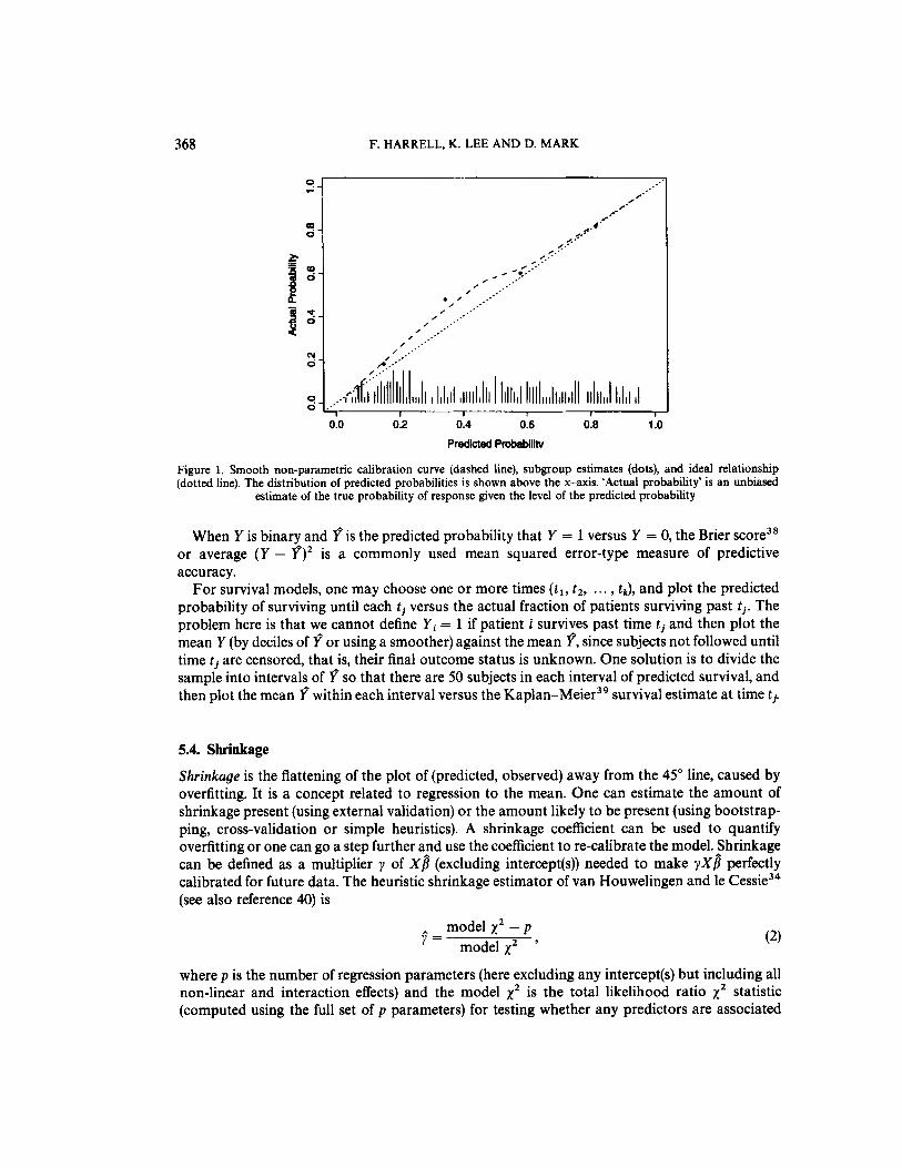
As an example, consider a 7-variable binary logistic regression model to predict the probability that a certain disease is present. The model was developed on a simulated 200-subject dataset of whom 93 had a final diagnosis that is positive. While fixing the intercept and 7 regression coefficients estimated from the training sample, predictive probabilities of disease were computed for each of 200 subjects in a separate sample, of whom 104 had the disease. The non-parametric calibration curve was estimated using a local least squares scatterplot smoother36 with the S-Plus function 10wess,~~ using the ‘no iteration’ option. The smoothed calibration graph is shown in Figure 1. Also shown is the proportion of patients with disease, grouped by intervals of predicted probability each containing 50 patients.

Note the typical regression to the mean effect caused by overfitting: predicted probabilities in the range of 0.3 to 0 5 are too low. Actual probabilities are closer to the mean (104/200 = 0.52).

368 F. HARRELL, K. LEE A N D D. MARK

0.0 0.2 0.4 0.6 0.8 1 .o Predicted Probabllihl

Figure 1. Smooth non-parametric calibration curve (dashed line), subgroup estimates (dots), and ideal relationship (dotted line). The distribution of predicted probabilities is shown above the x-axis. ‘Actual probability’ is an unbiased

estimate of the true probability of response given the level of the predicted probability

When Y is binary and f is the predicted probability that Y = 1 versus Y = 0, the Brier score3* or average ( Y - f)’ is a commonly used mean squared error-type measure of predictive accuracy.

For survival models, one may choose one or more times ( t l , tz, ... , tk), and plot the predicted probability of surviving until each t j versus the actual fraction of patients surviving past ti. The problem here is that we cannot define Yi = 1 if patient i survives past time ti and then plot the mean Y (by deciles of f or using a smoother) against the mean f, since subjects not followed until time t j are censored, that is, their final outcome status is unknown. One solution is to divide the sample into intervals of f so that there are 50 subjects in each interval of predicted survival, and then plot the mean f within each interval versus the Kaplan-Meier3’ survival estimate at time ti.

5.4. Shrinkage

Shrinkage is the flattening of the plot of (predicted, observed) away from the 45” line, caused by overfitting. It is a concept related to regression to the mean. One can estimate the amount of shrinkage present (using external validation) or the amount likely to be present (using bootstrapping, cross-validation or simple heuristics). A shrinkage coefficient can be used to quantify overfitting or one can go a step further and use the coefficient to re-calibrate the model. Shrinkage can be defined as a multiplier y of X g (excluding intercept@)) needed to make y X f l perfectly calibrated for future data. The heuristic shrinkage estimator of van Houwelingen and le Cessiej4 (see also reference 40) is

(2) model x 2 - p

j?= model xz ’

where p is the number of regression parameters (here excluding any intercept@) but including all non-linear and interaction effects) and the model xz is the total likelihood ratio xz statistic (computed using the full set of p parameters) for testing whether any predictors are associated


with Y! For linear regression, van Houwelingen and le Cessie’s heuristic shrinkage estimate reduces to the ratio of the adjusted R 2 to the ordinary R2 (derivable from reference 34, Eq. 70).

As an example, suppose that an analyst has considered 10 predictor variables, 6 of which were allowed to enter the model non-linearly (with 2 non-linear terms for each), and tested 8 interaction terms, for a total of 30 degrees of freedom. The model x2 is 100 for the full model fit with p = 30 d.f. The expected shrinkage is 0.70, indicating that about 0.3 of the model fit is ‘noise’. The ‘final model’ obtained from forward variable selection contains only 3 significant coefficients and has x2 = 81, but overfitting is quantified using the 30 candidate d.f. In this example, the number of variables, transformations, and interactions tried was too many for the sample size, and the resulting model is expected to be unstable. As a rough estimate, 0.3 of what was learned from developing the model was really non-replicable noise.

For mild overfitting in the case where the model is needed only to rank likely outcomes and not predict absolute risks, shrinking the regression coefficients will not help since it will not increase real discrimination. If the model is badly overfitted, the model may actually have negative (worse than random) discrimination on new data, and it will have poor calibration. The following heuristic strategy can then be used to determine whether data reduction is likely to result in a model that has any discrimination and how much reduction is required to yield reliable non-shrunken predictions.

First, fit a full model with all candidate variables, non-linear terms, and hypothesized interactions. Let p denote the number of parameters in this model, aside from any intercept(s). Let LR denote the likelihood ratio x z for this full model. The estimated shrinkage is (LR - p)/LR. If this falls below 0.85, for example, we may be concerned. Let q denote the regression degrees of freedom for a reduced model. In a ‘best case’, the variables removed to arrive at the reduced model would have no association with Y. The expected value of the x 2 statistic for testing those variables would then be p - q. The shrinkage for the reduced model is then on average [LR - (p - q) - q]/[LR - (p - q)] . Solving for q gives 4 < (LR - p)/9. Therefore, reduction of dimensionality down to q degrees of freedom would be expected to achieve < 10 per cent shrinkage. With these assumptions, there is no hope that a reduced model would have acceptable calibration unless LR > p + 9. If the information explained by the omitted variables is less than one would expect by chance (for example, their total x 2 is extremely small), a reduced model could still be beneficial, as long as the conservative bound (LR - q)/LR > 0-9 or q < LR/10 were achieved. This conservative bound assumes that no x 2 is lost by the reduction, that is, that the final model x2 GZ LR. This is unlikely in practice, since the data reduction must be only X-driven.

As an example, suppose that a binary logistic model is being developed from a sample containing 45 events on 150 subjects. A 10: 1 events: d.f. rule suggests we can analyse 4.5 degrees of freedom. The analyst wishes to analyse age, sex, and 10 other variables. It is not known whether interaction between age and sex exists, and whether age is linear. A restricted cubic spline is fitted with 4 knots (requiring two non-linear terms), and a linear interaction is allowed between age and sex. These two variables then need 3 + 1 + 1 = 5 degrees of freedom. The other 10 variables are assumed to be linear and to not interact with themselves or age and sex. There is a total of 15 d.f. The full model with 15 d.f. has LR = 50. Expected shrinkage from this model is

When stepwise fitting is done, the definition of p is confusing. Many analysts act as if the final model chosen with stepwise variable selection was pre-specified, whether interpreting R’, confidence limits, or P-values. For estimating the likely shrinkage, it has been shown that p is much closer to the number of candidate d.f. than to the number of parameters fitted in a ‘final’ model.40 On a similar note, reference 18 showed how to adjust a linear test of association for having done a test of quadratic effect, concluding that testing the single d.f. statistic for association as if it had 2 d.f. is nearly optimal.


(50 - 15)/50 = 0.7. Since LR > 15 + 9 = 24, some reduction might yield a better validating model. Reduction to q = (50 - 15)/9w4 d.f. would be necessary, assuming the reduced LR is about 50 - (15 - 4) = 39. In this case the 10: 1 rule yields about the same value for q. The analyst may be forced to assume that age is linear, modelling 3 d.f. for age and sex. The other 10 variables would have to be reduced to a single variable using principal components or another scaling technique. This single variable may not be interpretable, but using a single score is better than deleting all 10 variables from consideration. If the goal of the analysis is to make a series of hypothesis tests (adjusting P-values for multiple comparisons) instead of to predict future responses, the full model would have to be used.

B~o t s t r app ing~~ and cro~s-validation~~ may also be used to estimate shrinkage factors. As mentioned above, shrinkage estimates are useful in their own right for quantifying overfitting, and they are also useful for ‘tilting’ the predictions so that the (predicted, observed) plot does follow the 45” line, by multiplying all of the regression coefficients by 9. However, for the latter use it is better to follow a more rigorous approach such as penalized maximum likelihood estimation,” which allows the analyst to shrink different parts (for example, non-linear terms or interactions) of the equation more than other parts.42

5.5. General discrimination index

Discrimination can be defined more uniquely than calibration. It can be quantified with a measure of correlation without requiring the formation of subgroups or requiring smoothing.

When dealing with binary dependent variables or continuous dependent variables that may be censored when some patients have not suffered the event of interest, the usual mean squared error-type measures do not apply. A c (for concordance) index’ is a widely applicable measure of predictive discrimination - one that applies to ordinary continuous outcomes, dichotomous diagnostic outcomes, ordinal outcomes, and censored time until event response variables. This index of predictive discrimination is related to a rank correlation between predicted and observed outcomes. It is a modification of the Kendall--Goodman-Kruskal-Somers type rank correlation index43 and was motivated by a modification of Kendall’s z by Brown et ~ 1 . ~ ~ and Schemper?’

The c index is defined as the proportion of all usable patient pairs in which the predictions and outcomes are concordant. The c index measures predictive information derived from a set of predictor variables in a model. In predicting the time until death, c is calculated by considering all possible pairs of patients, at least one of whom has died. If the predicted survival time is larger for the patient who lived longer, the predictions for that pair are said to be concordant with the outcomes. If one patient died and the other is known to have survived at least to the survival time of the first, the second patient is assumed to outlive the first. When predicted survivals are identical for a patient pair, rather than 1 is added to the count of concordant pairs in the numerator of c. In this case, one is still added to the denominator of c (such patient pairs are still considered usable). A patient pair is unusable if both patients died at the same time, or if one died and the other is still alive but has not been followed long enough to determine whether she will outlive the one who died.

Instead of using the predicted survival time to calculate c, the predicted probability of surviving until any fixed time point can be used equivalently, as long as the two estimates are one-to-one functions of each other. This holds for example if the proportional hazards assumption is satisfied.

For predicting binary outcomes such as the presence of disease, c reduces to the proportion of all pairs of patients, one with and one without the disease, in which the patient having the disease had the higher predicted probability of disease. As before, pairs of patients having the same


predicted probability get 3 added to the numerator. The denominator is the number of patients with disease multiplied by the number without disease. In this binary outcome case, c is essentially the Wilcoxon-Mann-Whitney statistic for comparing predictions in the two outcome groups, and it is identical to the area under a receiver operating characteristic (ROC) c ~ r v e . ~ ~ * ~ ' Liu and Dyer4' advocate the use of rank association measures such as c in quantifying the impact of risk factors in epidemiologic studies.

The c index estimates the probability of concordance between predicted and observed responses. A value of 0.5 indicates no predictive discrimination and a value of 1.0 indicates perfect separation of patients with different outcomes. For those who prefer instead a rank correlation coefficient ranging from - 1 to + 1 with 0 indicating no correlation, Somers' D rank correlation index is derived by calculating 2(c - 03) . Either c or the rank correlation index can be used to quantify the predictive discrimination of any quantitative predictive method, whether the response is continuous, ordinal, or binary.

Even though rank indexes such as c are widely applicable and easily interpretable, they are not sensitive for detecting small differences in discrimination ability between two models. This is due to the fact that a rank method considers the (prediction, outcome) pairs (0.01,0), (0.9, 1) as no more concordant than the pairs (0.05,0), (0.8, 1). A more sensitive likelihood-ratio X2-based statistic that reduces to R2 in the linear regression case may be s u b s t i t ~ t e d . ~ ~ - ~ ' Korn and Simons2 have a very nice discussion of various indexes of accuracy for survival models.

6. MODEL VALIDATION METHODS

As mentioned before, examination of the apparent accuracy of a multivariable model using the training dataset is not very useful. The most stringent test of a model (and of the entire data collection system) is an external validation - the application of the 'frozen' model to a new population. It is often the case that the failure of a model to validate externally could have been predicted from an honest (unbiased) 'internal' validation. In other words, it is likely that many clinical models which failed to validate would have been found to fail on another series of subjects from the original source, because overfitting is such a common problem. The principal methods for obtaining nearly unbiased internal assessments of accuracy are data-~plitting,~~ cross-ualida- lions4 and bootstr~pping.~"~~ In data-splitting, a random portion, for example 5, of the sample is used for all model development (data transformations, stepwise variable selection, testing interactions, estimating regression coefficients, etc.). That model is 'frozen' and applied to the remaining sample for computing calibration statistics, c, etc. The size of the validation sample must be such that the relationship between predicted and observed outcomes can be estimated with good accuracy, and the remaining data are used as the training (model development) sample. Data- splitting is simple, because all the modelling steps, which may include subjective judgements, are only done once. Data-splitting also has an advantage when it is feasible to make the single split with respect to geographical location or time, resulting in a more stringent validation that demonstrates generalizability. However, in addition to severe difficulties listed below, data splitting does not validate the final model, if one desires to recombine the training and test data to derive a model for others to use.

Cross-validation is repeated data-splitting. To obtain accurate estimates using cross-validation, more than 200 models may need to be developed and tested,54 with results averaged over the 200 repetitions. For example, in a sample of size n = 1O00, the modelling process (all components of it!) could be done 400 times, leaving out a random 50 subjects each time and developing the model on the 950 remaining subjects. The benefits of cross-validation over data-splitting are


clear; the size of the training samples can be much larger, so less data are discarded from the estimation process. Secondly, cross-validation reduces variability by not relying on a single sample split.

Efron has shown that cross-validation is relatively inefficient due to high variation of accuracy estimates when the entire validation process is re~eated.~” Data-splitting is far worse; the indexes of accuracy will vary greatly with different splits. Bootstrapping is an alternative method of internal validation that involves taking a large number of samples with replacement from the original sample. Bootstrapping provides nearly unbiased estimates of predictive accuracy that are of relatively low variance, and fewer model fits are required than cross-validation. Bootstrapping has an additional advantage that the entire dataset is used for model development. As others have shown, data are too precious to waste.59s60

Suppose that we wish to estimate the expected value (for new patient samples similar to the derivation sample) of the Somers’ D rank correlation coefficient between predicted and observed survival time. The following steps can be used (see references 55, 58 and 60 for the basic method when applied to binary outcomes):

1. Develop the model using all n subjects and whatever stepwise testing is deemed necessary. Let Dapp denote the apparent D from this model, i.e., the rank correlation computed on the same sample used to derive the fit.

2. Generate a sample of size n with replacement from the original sample (for both predictors and the response).

3. Fit the full or possibly stepwise model, using the same stopping rule as was used to derive Dam.

4. Compute the apparent D for this model on the bootstrap sample with replacement. Call it

5. ‘Freeze’ this reduced model, and evaluate its performance on the original dataset. Let

6. The optimism in the fit from the bootstrap sample is Dbool - Dorip. 7. Repeat steps 2 to 6 10Ck200 times. 8. Average the optimism estimates to arrive at 0. 9. The bootstrap corrected performance of the original stepwise model is D,,, - 0. This

difference is a nearly unbiased estimate of the expected value of the external predictive discrimination of the process which generated DapV In other words, Dapp - 0 is an honest estimate of internal validity, penalizing for overfitting.

Dboot.

Dorig denote the D.

As an example, suppose we want to validate a stepwise Cox model developed from, say, a sample of size n = 300 with 30 events. The candidate regressors are age, age2, sex, mean arterial blood pressure (MBP), and a non-linear interaction between age and sex with the terms age x sex and age2 x sex. MBP is assumed to be linear and additive. Denote these variables by the numbers 1-6. The model x2 is 45 with 6 d.f., so the approximate expected shrinkage is = 0.87, or 0-13 overfitting, so some caution needs to be exercised in using the estimated model coefficients and hence in using extreme predicted survival probabilities without calibration (shrinkage). The D for the full model is 0.42. A step-down variable selection using Akaike’s information criterion (AIC)34*61 as a stopping rule (x2 for set of variables tested > 2 x d.f.) resulted in a model with the variables age, age’, sex, age x sex. The reduced model had D = 0.39, a typical loss due to deleting marginally important but statistically insignificant variables. Two-hundred bootstrap repetitions are done, repeating the variable selection for each sample using the same stopping rule. We want to detect whether the D = 0.39 is likely to validate in a new series of subjects from the same population. The first five samples might yield the results shown in Table I.


Table I. Example validation of predictive discrimination

Re-sample Dboot Variables retained D b O O l Dorip Optimism Full model Reduced model

1 0.45 1,2,3,5,6 044 037 0.07 2 0.46 172 0.34 030 0.04 3 0.42 1,Z 3,4 0.37 0.34 0.03 4 043 1,2,3,5 0.42 039 0.03 5 0.41 1,3,4 0.39 037 002

The average optimism is 0.038, so the bootstrap estimate of the expected validation of D,,, is 0.39 - 0.038 = 0.352. The analyst may or may not be worried about the 0.038 overfitting, but the best estimate of predictive discrimination is D = 0.352 - this is a better estimate of the likely ‘external’ validation accuracy than is 0-39 if all other aspects of the study design remain constant. The D = 0.352 is the honest estimate of predictive accuracy that should be quoted when the researchers document the accuracy of the reduced model that was developed on the entire dataset using a stepwise variable selection algorithm.

It is usually informative to repeat the bootstrap validation with and without stepwise variable selection. Usually, the amount of predictive information lost by deleting marginal variables is not offset by the decreased optimism of the stepwise model. One way to demonstrate this point is to observe how often ‘insignificant’ clinical predictors have clinically sensible signs on their regression coefficients. Stepwise variable selection, which requires binary decisions about the inclusion of variables (unlike shrinkage), causes information to be lost.2

The same strategy can be used to estimate the over-optimism in an R2 measure49 from the original model fit. For estimating the prediction error at time t in a survival model, similar steps could also be used. Instead of validating a correlation D, we substitute for example the statistic D = difference between mean predicted 2-year survival probability and Kaplan-Meier 2-year survival estimate. The survival estimates are made by, say, deciles of predicted 2-year survival from the original model fit using the following steps, for example:

1. Develop the model using all subjects. 2. Compute cut points on predicted survival at 2 years so that there are m patients within each

interval (m = 50 or 100 typically). 3. For each interval of predicted probability, compute the mean predicted 2-year survival and

the Kaplan-Meier 2-year survival estimate for the group. 4. Save the apparent errors - the differences between mean predicted and Kaplan-Meier

survival. 5. Generate a sample with replacement from the original sample. 6. Fit the full model. 7. Do variable selection and fit the reduced model. 8. Predict 2-year survival probability for each subject in the bootstrap sample. 9. Stratify predictions into intervals using the previously chosen cut points.

10. Compute Kaplan-Meier survival at 2 years for each interval. 11. Compute the difference between the mean predicted survival within each interval and the

12. Predict 2-year survival probability for each subject in the original sample using the model Kaplan-Meier estimate for the interval.

developed on the sample with replacement.

374

13.

14.

15. 16.

17.

1.

2.

3.

4.

c

F. HARRELL, K. LEE AND D. MARK

For the same cut points used before, compute the difference in the mean predicted 2-year survival and the corresponding Kaplan-Meier estimates for each group in the original sample. Compute the differences in the differences between the bootstrap sample and the original sample. Repeat steps 5 to 14 100-200 times. Average the 'double differences' computed in step 14 over the 100-200 bootstrap samples. These are the estimates of over-optimism in the apparent error estimates. Add these over-optimism estimates to the apparent errors in the original sample to obtain bias-corrected estimates of predicted versus observed, that is, to obtain a bias- or overfitting-corrected calibration curve.

7. SUMMARY O F MODELLING STRATEGY

Assemble accurate, pertinent data and as large a sample as possible. For survival time data, follow-up must be sufficient to capture enough events as well as the clinically meaningful phases if dealing with a chronic disease. Formulate focused clinical hypotheses that lead to specification of relevant candidate predictors, the form of expected relationships, and possible interactions. Discard observations having missing Y after characterizing whether they are missing at random." See reference 62 for a study of imputation of Y when it is not missing at random. If there are any missing X s , analyse factors associated with missingness. If the fraction of observations that would be excluded due to missing values is very small, or one of the variables that is sometimes missing is of overriding importance, exclude observations with missing values". Otherwise impute missing X s using individual predictive models that take into account the reasons for missing, to the extent possible.

>. If the number of terms fitted or tested in the modelling process (counting non-linear and cross-product terms) is too large in comparison with the number of outcomes in the sample, use data reduction (ignoring Y)20-23 until the number of remaining free variables needing regression coefficients is tolerable. Assessment of likely shrinkage (overfitting) can be useful in deciding how much data reduction is adequate. Alternatively, build shrinkage into the initial model fitting."

6. Use the entire sample in the model development as data are too precious to waste. If steps listed below are too difficult to repeat for each bootstrap or cross-validation sample, hold out test data from all model development steps which follow.

7. Check linearity assumptions and make transformations in X s as needed. 8. Check additivity assumptions and add clinically motivated interaction terms. 9. Check to see if there are overly-influential observation^.^' Such observations may indicate

overfitting, the need for truncating the range of highly skewed variables or making other pre-fitting transformations, or the presence of data errors.

'I For survival time data, no observations should be missing on Y. They should only have curtailed follow-up. Alternatively, impute missing values for the predictor but perform secondary analyses later to estimate the strength of

association between X and Y after deleting observations with that predictor imputed, as imputation will attenuate the relationship.


10. Check distributional assumptions and choose a different model if needed (in the case of Cox models, stratification or time-dependent covariables can be used if proportional hazards is violated).

11. Do limited backwards step-down variable selection.63 Note that since stepwise techniques do not really address overfitting and they can result in a loss of information, full model fits (that is, leaving all hypothesized variables in the model regardless of P-values) are frequently more discriminating than fits after screening predictors for s i g n i f i ~ a n c e . ~ . ~ ~ They also provide confidence intervals with the proper coverage, unlike models that are reduced using a stepwise p r o ~ e d u r e , ~ ~ . ~ ~ . 6 5 fr om which confidence intervals are falsely narrow. A compromise would be to test a pre-specified subset of predictors, deleting them if their total x2 c 2 x d.f. If the x2 is that small, the subset would likely not improve model accuracy.

12. This is the ‘final’ model. 13. Validate this model for calibration and discrimination ability, preferably using bootstrap-

ping. Steps 7 to 11 must be repeated for each bootstrap sample, at least approximately. For example, if age was transformed when building the final model, and the transformation was suggested by the data using a fit involving age and age2, each bootstrap repetition should include both age variables with a possible step-down from the quadratic to the linear model based on automatic significance testing at each step.

14. If doing stepwise variable selection, present a summary table depicting the variability of the list of ‘important factors’ selected over the bootstrap samples or cross-validations. This is an excellent tool for understanding why data-driven variable selection is inherently ambiguous.

15. Estimate the likely shrinkage of predictions from the model, either using equation (2) or by bootstrapping an overall slope correction for the prediction^.^^ Consider shrinking the predictions to make them calibrate better, unless shrinkage was built-in. That way, a predicted 0.4 mortality is more likely to validate in a new patient series, instead of finding that the actual mortality is only 0.2 because of regression to the mean mortality of 0.1.

8. SOFTWARE

Modern statistical software such as S-Plus3’ on UNIX workstations makes it quite feasible to perform the extensive calculations required to do the recommended model building steps. The first author has written a package of UNIX S-Plus functions called Design66 that allow the analyst to perform all analyses mentioned here including tests of linearity, pooled interaction tests, model validation and graphical methods for interpreting models. Here are some examples:

# First find optimum transformations relating each predictor to each # other, and use multiple regression in these transformations to # impute missing values. Use shrinkage to avoid over-imputing trans t transcan( - age + cholesterol + sys. bp + weight, imputed = T, shrink = T) cholesterol +- impute(trans, cholesterol) # impute missings sys . bp + impute(trans, sys . bp) # Fit a Cox P.H. model allowing some interactions with age and # nonlinearity in cholesterol and sys . bp using restricted cubic splines # x = T, y = T means store data in fit for future bootstrapping fit + cph(Surv(fu.time, death) - age * (rcs(cholestero1) + rcs(sys.bp)) +

anova(fit) fastbw(fit) # fast backward step-down

weight, x = T, y = T, sw = T, t i m 0 . h ~ = 5) # automatic pooled Wald tests


Table 11. Candidate predictors and d.f.

Predictor Name Number of Original levels parameters

~~~~~

Dose of oestrogen Age in years Weight index: wt(kg) - ht(cm) + 200 Performance rating

History of cardiovascular disease Systolic blood pressure/lO Diastolic blood pressure/ 10 Electrocardiogram code

Serum haemoglobin (g/lOO mi) Tumour size (cm2) Stage/histologic grade combination Serum prostatic acid phosphatase Bone metastasis

placebo, 02, 1.0, 50 mg oestrogen

normal, in bed <50% of time, in bed >SO%, in bed always

present /absent

normal, benign, rhythm disturbance, block, strain, old myocardial infarct, new MI

present / absent

# Next validate model, penalizing for backward stepdown variable selectlon Vdidatdfit, B = 100, bw = T) ccL.librate(fit, B = 100, bw = T, u = 5) # bias-corrected 6-yr survival calibration plot(summary(fit)) nomogram(fit> latex(fit) # typeset model equation

# bootstrap validation of adzuracy indexes

# plot hazard ratios with confidence Urnits # draw nomogram displaying how model works

The Design library includes a function rcorr.cens for computing the general c-index, and the function va,l.prob which produced Figure 1 and also prints a variety of accuracy measures. For binary and ordinal logistic models and for ordinary linear models, Design has a general penalized maximum likelihood estimation facility. Design is available in the statlib repository (Internet address Lib. stat. cmu. edu). transcan and impute are separate functions in statlib which work on UNIX as well as DOS Windows S-Plus. Some other software systems which have some intermediate-level capabilities include Stata (Computer Resources Center Inc., College Station TX), SPIDA (NHMRC Clinical Trials Centre, Eastwood, NSW Australia), and SAS (SAS Institute Inc., Cary NC).

9. CASESTUDY

Consider the 506-patient prostate cancer dataset from Byar and Green6’ which has also been analysed in references 68 and 69. The data are listed in reference 70, Table 46, and are available by Internet at utstat. toronto. edu in the directory /pub/data-collect. These data were from a randomized trial comparing four treatments for stage 3 and 4 prostate cancer, with almost equal numbers of patients on placebo and each of three doses of oestrogen. Four patients had missing values on all of the following variables: wt, pf, hx, sbp, dbp, ekg, hg, bm; two of these patients were also missing sz (see Table I1 for abbreviations). These patients will be excluded from consideration.

There are 354 deaths among the 502 patients. If we only wanted to test for a drug effect on survival time, a simple rank-based analysis would suffice. To be able to test for differential treatment effect or to estimate prognosis or expected absolute treatment benefit for individual


patients, however, we need a multivariable survival modeL3 First we consider fitting a full additive model which does not assume linearity of effect for any predictor. Categorical predictors will be expanded using dummy variables. For pf we could lump the last two categories since the last category has only two patients. Likewise, we could combine the last two levels of ekg. Continuous predictors will be expanded by fitting 4-knot restricted cubic spline functions, which contain two non-linear terms and thus have a total of 3 d.f. Table I1 defines the candidate predictors and lists their d.f. The variable stage is not listed as it can be predicted with high accuracy from sz, sg, ap, bm (stage could have been used as a predictor for imputing missing values on sz, sg).

There are a total of 36 candidate d.f. which should not be artificially reduced by ‘univariable screening’ or graphical assessments of association with death. This is about &j as many predictor d.f. as there are deaths, so there is some hope that a fitted model may validate. Let us also examine this issue by estimating the amount of shrinkage using equation (2). We use a Cox proportional hazards model for time until death. The UNIX S-Plus Design library fits the full model using restricted cubic spline expansions and makes use of Therneau’s survival4 package in statlib” to perform the calculations. First we invoke the transcan function and impute functions (from statlib for any versions of S-Plus) to develop customized non-linear imputation equations for all predictors and to apply these equations to impute missing values.

# Define function for easy determination of whether a value is in a list ‘%in% +- function (a, b) match (a, b, nomatch = 0) > 0

levels(ekg) [levels(ekg) %in% c(’o1d MI’,’recent MI’)] +- ’MI’ # combines last 2 levels and uses a new name, MI

pf.coded + as.integer(pf) # save origind pf, re-code to 1-4 levels(pf) + c(levels(pf) [ 1 : 31, levels(pf) [3]) # combine last 2 levels of originaJ w

sz + impute(w,sz) # we8 imputation rule w sg + -Puww, sf3 age + impute(w, age) wt e impute(w,wt) ekg + impute(w, ekg)

dd + datadist(rx, age, wt, pf, pf.coded, heart, map, hg, 82, sg, ap, bm) options(datadist = ’dd’)

units(dtime) + ’Month’ S t Surv(dtime, sbtusl= ’alive’)

f t cph(S - rx + rcs(age,4) + rcs(wt,4) + pf + hx + rcs(sbp,4) + rcs(dbp,4) + ekg + rcs(hg,4) + rcs(sg,4) + rcs(sz,4) + rcs(ap,4) + bm)

+ transcan<- sz + sg + ap + sbp + dbp + age + wt + hg + ekg + pf + bm + hx, imputed = T, impcat = ’tree’)

# d a W s t stores characteristlcs of raw data

The likelihood ratio x2 statistic is 140 with 36 d.f. This test is highly significant so some modelling is warranted. The AIC value (on the x2 scale) is 140 - 2 x 36 = 68. The rough shrinkage estimate is 0.743 (104/140) so we estimate that 26% of the model fitting will be noise, especially with regard to calibration accuracy. The approach of reference 2 is to fit this full model and to shrink predicted values. We will instead try to do data reduction (blinded to individual x2 statistics from the above model fit) to see if a reliable model can be obtained without shrinkage. A good approach at this point might be to perform a variable clustering analysis which for our purposes we will do informally. The data reduction strategy is listed in Table 111. For ap, more exploration is desired to be able to model the shape of effect with such a highly skewed


Table 111. Data reduction strategy (blinded to Y)

Variables Reductions d.f. saved

wt

Pf Assume linearity hx, ehg

Assume variable not important enough for 4 knots Use 3 knots

Make new 0,1,2 variable and assume linearity: 2 = hx and ekg not normal and benign, 1 = either, 0 = none Combine into mean arterial bp and use 3 knots: map = + dpb + f spb

sbp, dbp

sg Use 3 knots 82 Use 3 knots aP Look at shape of effect of ap in detail, -

and take log before expanding in spline to achieve numerical stability: add 2 knots

1

1 5

4

1 1

-2

distribution. Since we expect the tumour variables to be strong prognostic factors we will retain them as separate variables. No assumption will be made for the dose-response shape for oestrogen, as there was reason to expect a non-monotonic effect due to competing risks for cardiovascular death.

heart + hx + I (ekg %in% c('normal','benign')) label(heart) + 'Heart Disease Code' map + (2rdbp + sbp)/3 IabeKmap) + 'Mean Arterial Pressure/ 10'

f + cph(S - rx + rcs(age,4) + rcs(wt,3) t pf.coded + heart + rcs(map,3) + rcs(hg,4) +

x = T, y = T, BW = T, time. inc = 5 * 12) rCS(Sg,3) + I'CS(S2,3) + rcs(log(ap),d) + bm,

# x, y for predict, validate, calibrate; BUPV, time. inc for calibrate

The total savings is thus 11 d.f. The likelihood ratio x2 is 126 with 25 f . , with a ! ighi Y improved AIC of 76. The rough shrinkage estimate is slightly better at 080, but still worrisome. A further data reduction might be achieved by using the transcan transformations determined from self-consistency of predictors, but we will stop here and use this model.

Now assess this model in more detail by examining coeflicients and summarizing multiple parameters within predictors using Wald statistics.

f

Cox Proportional Hazards Model

cph<formula = S - IX + rcscage, 4) + rcscwt, 3) + pf.coded + heart + rcs(map, 3) +

# writing an object name in 8 causes it to be printed

rca(hg, 4) + W<SZ, 3) t rcscsg, 3) + rcs(log(ap), 6) + bm, x = T, y = T, BW = T, time.inc = 6 + 12)

Obs Events Model L.R. d.f. P Score Score P R 2 502 354 126 26 0 136 0 0.221

coef se(coen z P rx = 02mg estrogen 3.740 - 03 1.500 - 01 0.0260 9.800 - 01 rx = 1.Omg estrogen -4.210 - 01 1.660 - 01 -2.6427 1,100 - 02 rx = 8.Omg estrogen -9736 - 02 1.580 - 01 -06176 537e - 01

age -1.170-02 2.350-02 -0.4996 6.17e-01 age' 2-000 - 02 8-868 - 02 0'5190 0.040 - 01


age” wt wt’

pf . coded heart map map’ hB hg‘

hg”

sz’ sg

sg’ aP

aP’ ap’ ’

ap’ ’ ’ ,P””

bm

8Z

2.7le - 01 -2.46e - 02

1.848 - 02 2.28e - 01 4.18e - 01 3.24e - 02

-4437e - 02 - 1B6e - 01

7.42e - 02 8.08e - 01 1.00e - 02 879e - 03 7.19e - 02

-7.04e - 03 -F96e - 01

4.89e + 01 -3.64e + 02

4.04e + 02 -9.69e + 01

328e - 02

498e - 01 9.398 - 03 1.12e - 02 1.21~3 - 01 8.08e - 02 8.498 - 02 9.41~1- 02 7.68e - 02 2.10e - 01 1.27e + 00 1.44e - 02 2.37e - 02 7.86e - 02 9.83~1- 02 3 l l e - 0 1 2.18e + 01 1.89e + 02 1.78e + 02 4.16e + 01 1.81e - 01

0.8482

1.6379 1.8628 8.1 723 0.38 1 7

-2.6178

-0.4887 -2.0343

0.3830 0.40 14 0.6988 0.37 18 0.9 138

-0.07 16 -2.8884

2.2482

23087 - 2.33 1 1

0.1790

-2.2909

8.84e - 0 1 8.86e - 03 1.01e - 01 628e - 02 2.31~1- 07 7.03e - 01 6.27e - 0 1 4.19~1- 02 7.24e - 0 1 688e - 0 1 4.87e - 0 1 7.10e - 0 1 3.61e - 0 1 9.43e - 0 1 1.05e - 02 2.46e - 02 2.20e - 02 2.1 le - 02 197e - 02 8.88e - 0 1

# The terms with ’, ”, etc. after the name are cubic spline nonllnear terms # The dose effect is apparently nonllnear.

anova(f ) # output waa actua3I.y typesetted automatkally wing latex(anova(f)) # latex requires the print.display package from statlib

There are 12 parameters associated with non-linear effects, and the overall test of linearity indicates the strong presence of non-linearity for at least one of the variables age, wt, map, hg, 82, sg, ap (see Table IV). There is a difference in survival time between at least two of the doses of oestrogen.

Now that we have a tentative model, let us examine the model’s distributional assumptions. As mentioned in Section 4.3, the Schoenfeld partial residuals are an effective tool for checking the proportional hazards assumption in the Cox model. Grambsch and T h e r n e a ~ ’ ~ have modified these residuals so that smoothed plots of them estimate the effect of predictors on the log instantaneous hazard rate as a function of follow-up time. Their scaled residuals estimate B(t), the regression coefficient as a function of time. A messy detail is how to handle multiple regression coefficients per predictor. Here we do an approximate analysis in which each predictor is scored by adding up all the terms in the model to transform that predictor to be optimally related to the log hazard (at least if the shape of the effect does not change with time). In doing this we are temporarily ignoring the fact that the individual regression coefficients were estimated from the data. For dose of oestrogen, for example, we code the effect as 0 (placebo), 0.0037 (0*2mg), -0.421 (1.0 mg), and -0.0973 (5.0 mg), and age is transformed as -0.0117 age + 0.02 age’ + 0-271 age”, which in most simple form is

- 1.17 x 10-2age + 3.48 x 10- ’(age - 56): + 4.71 x lO-*(age - 71):

where (x) + means to ignore that term if x < 0, and the knots for age are 56,71,75 and 80 years. In S-Plus the predict function easily summarizes multiple terms and produces a matrix (here,

z) containing the total effects for each predictor. Matrix factors can easily be included in model


Table IV. Wald statistics for S

x 2 d.f. P

rx age

wt

pf. coded heart map

hg

Non-linear

Non-linear

Non-linear

Non-linear

Non-linear

Non-linear

Non-linear

sz

sg

aP

bm

TOTAL TOTAL NON-LINEAR

8.38 12.85 8.18 8.87 2.68 3.47

26.75 0.25 0.24

11.85 6.92

10.60 0.14 3.14 0.01

13.17 12.93 0.03

30.28 128.08

3 3 2 2 1 1 1 2 1 3 2 2 1 2 1 5 4 1

12 25

0.0387 0.0050 0.0168 00118 01014 0.0625

<O.OOol 043803 0.6272 0.0079 0.03 14 0.0050 0.7102 0.2082 0.9429 0.0218 0.01 16 0.8579 04025

<OOOO1

formulae.

z t predic-(f, type = ’terms’) # required x = T above to store cdsign # matrix

f . short + cph(S - z, x = T, y = T) # store x, y so can get residuals The fit f.short based on the matrix z of single d.f. predictors has the same LR xz of 126 as the fit f, but with a falsely low 11 d.f. All regression coefficients are unity.

Now get scaled Schoenfeld residuals separately for each predictor and test the proportional hazards assumption for each using the ‘correlation with time’ test. Also plot smoothed trends in the residuals. The plot method for cox. zph objects uses restricted cubic splines to smooth the relationship.

phtest + cox. zph(f . short, transform = ’identity’) phtest

rho chisq P r~ 0.12965 6.8481 0.0 108

age -0.08911 2.8518 0.09 13 wt -0.00878 0.0269 0.8697

pf. Coded -0.06238 1.4278 0.232 1 heart 0*01017 0.0451 0.83 19 map 0.03928 0.4998 0.4796 hg -0.06678 1.7368 0.1876 SZ -0.08262 09834 0.32 14 Sg -0.04276 0.6474 0.42 10 ap 0.01237 0.0858 0.8 133 bm 0.04891 0.9241 0.3364

GLOBAL NA 18.3776 0.1659

MULTIVARIABLE PROGNOSTIC MODELS 38 1

. I I I

0 20 40 60

Time

Figure 2. Raw and spline-smoothed scaled Schoenfeld residuals for dose of oestrogen, non-linearly coded from the Cox model fit, with 2 standard error^.'^

Only the drug effect significantly changes over time (P = 0.01 for testing the correlation rho between the scaled Schoenfeld residual and time), but when a global test of PH is done penalizing for 11 d.f., the P-value is 0.17. A graphical examination of the trends does not find anything interesting for the last 10 variables. A residual plot is drawn for rx alone and is shown in Figure 2.

plot(phtest, var = 'rx')

We will ignore the possible increase in effect of oestrogen over time. If this non-PH is real, a more accurate model might be obtained by stratifying on rx or by using a time x rx interaction as a time-dependent covariable.

Note that the model has several insignificant predictors. These will not be deleted, as that would not improve predictive accuracy and it would make confidence intervals for a or for predicted survival probabilities with the correct coverage probabilities hard to obtain.64 At this point it would be reasonable to test pre-specified interactions. Here we will test all interactions with dose. Since the multiple terms for many of the predictors (and for rx) make for a great number of d.f. for testing interaction (and a loss of power), we will do approximate tests on the data-driven codings of predictors. P-values for these tests are likely to be somewhat anti- conservative.

z.dose +- z[,'rx'] # same aa s ~ z [ , l ] - get first column a . other + z [,-1] # aJl but the first column of z f.ia + cph(8 - z.dose * z.other) anova(f . ia)

Factor Chi-square d.f. P

z . other (Factor + Hlgher Order Factors) 134.3 20 0~000

z.dose (Factor + Higher Order Factors) 189 11 0.082 All Interactions 12.2 10 0.2'73

All Interactions 12.2 10 0.2'73 z . dose z. other (Factor + Higher Order Factors) 12.2 10 0.2'73 TOTAL 137.3 21 0.000


. . . 5.0mgertro 50 80 70 80

1 2 3 4 0 1 2

0 ....................

0 d -I:..:--:-.-> ..*.-” --- -..

9 r

8 10 12 14

Figure 3. Shape of each predictor on log hazard of death. Y-axis shows A’s, but the predictors not plotted are set to reference values. ‘Rug plots’ on the top of each graph show the data density of the predictor. Note the highly non-monotonic relationship with ap, and the increased slope after age 70 which has been found in outcome models for

various diseases

Here ‘Factor + Higher Order Factors’ means the combined main effect and interaction effect. The global test of additivity has P = 0.27, so we will ignore the interactions (and also forget to penalize for having looked for them below!).

The following UNIX S-Plus statements plot how each predictor is related to the log hazard of death, along with 0.95 confidence bands. Note that due to a peculiarity of the Cox model the standard error of the predicted X p is zero at the reference values (medians here, for continuous predictors).

pm(mfrow = ~(3,411 r + c ( - l , 1) plot (f, r~ = NA, plot (f, age = NA, scat 1 d(age> plot(f, wt = NA,

# 4 x 3 matrix of graph # use common y-exis range for all ylim = r) ylim = r)

ylim = r)

NA +use default range for predidor

# scatld from statlib, for any S-Plus # scatld shows data density

. . .


0.1 0.2 0.3 0.4 0.5 0.6

Predicted 60 Month Survival

Figure 4. Bootstrap estimate of calibration accuracy for 5-year estimates from the final Cox model. Dots correspond to apparent predictive accuracy. x marks the bootstrapcorrected estimates

We first validate this model for Somers’ D,, rank correlation between predicted log hazard and observed survival time, and for slope shrinkage. The bootstrap is used (with 200 re-samples) to penalize for possible overfitting, as discussed in Section 6.

validata(f, B = 200, = T, pr = T)

index. orig training test optimism index. n corrected

DXy -0.337377 -0‘384844 -0.30978 -0.03488 -0.28230 200 R2 0.221444 0.281369 0.18446 0.0769 1 0-14453 200 Slope 1 .OOOOOO 1 .OOOOOO 0,78484 0.2 1638 0.78464 200

Here ‘training’ refers to accuracy when evaluated on the bootstrap sample used to fit the model, and ‘test’ refers to the accuracy when this model is applied without modification to the original sample. The apparent D,, is -0.34, but a better estimate of how well the model will discriminate prognoses in the future is D,, = - 0.28. The bootstrap estimate of slope shrinkage is 0.78, surprisingly close to the simple heuristic estimate. The shrinkage coefficient could easily be used to shrink predictions to yield better calibration.

Finally, we validate the model (without using the shrinkage coefficient) for calibration accuracy in predicting the probability of surviving 5 years. As detailed in Section 5, the bootstrap is used to estimate the optimism in how well predicted 5-year survival from the final Cox model tracks Kaplan-Meier 5-year estimates, stratifying by grouping patients in subsets with about 70 patients per interval of predicted 5-year survival.

plot(ca,librate(f, B = 200, u = 6 * 12, m = 70))

The estimated calibration curves are shown in Figure 4. Bias-corrected calibration is very good except for the two groups with extremely bad prognosis - their survival is slightly better than predicted, consistent with regression to the mean. Even there, the absolute error is low despite a large relative error. Hence for this example it may not be worthwhile to develop a model using shrinkage.

Now compare this analysis with three previous analyses of this dataset. In all three analyses, all continuous covariables were arbitrarily categorized into intervals and scored with somewhat arbitrary category codes. In none of the three were sbp, dbp, ekg, ap, bm considered. Patients having missing values on any of the candidate predictors were excluded from consideration.

384 F. HARRELL. K. LEE AND D. MARK

Turn first to Byar and Green,67 who used an exponential survival model and dichotomized treatment by combining placebo and low dose and combining the two highest doses. The important predictors were found to be hx, sg, sz, hg, and the following interactions were detected in an exploratory analysis which did not control for multiple comparisons: rx x sg and IX x age. These interactions were not significant in the present model (even if dose were rexoded as in Byar and Green).

Kay6’ considered Cox models for various causes of death. For time until all-cause mortality, Kay found that the most important predictors were 82, hx, sg, age. The treatment along with age, hx were significant predictors of cardiovascular death. The treatment (in the opposite direction), and hg, sz, sg predicted cancer death. Treatment and age, w t predicted time until death from other causes.

Sauerbrei and SchurnacheP9 also used a Cox model and an approach in which a backward elimination procedure was done for each of 100 bootstrap samples. The relative frequency of selection of variables as ‘important’ was used as the criterion for inclusion of variables in the final model. Variables were retained if they were selected 2 70 times. All candidate predictors met this criterion. Treatment interactions involving age and sg were the most common interactions (56 and 48 bootstrap repetitions, respectively), but they did not meet the criterion for selection. The authors noted that these interactions were misleadingly more significant in a model which only adjusted for ‘significant’ predictors instead of all candidate predictors.

None of the three references just cited provided a model validation or quantified the predictive discrimination of the final model.

10. SUMMARY

Methods were described for developing clinical multivariable prognostic models and for assessing their calibration and discrimination. A detailed examination of model assumptions and an unbiased assessment of predictive accuracy will uncover problems that may make clinical prediction models misleading or invalid. The modelling strategy presented in Section 7 provides one sequence of steps for avoiding the pitfalls of multivariable modelling so that its many advantages can be realized.

ACKNOWLEDGEMENTS

This work was supported by research grants HL-17670, HL-29436, HL-36587, HL-45702 and HL-093 15 from the National Heart, Lung and Blood Institute, Bethesda, Maryland, research grants HS-03834, HS-05635, HS-06503, HS-06830, and HS-07137 from the Agency for Health Care Policy and Research, Rockville, Maryland, and grants from the Robert Wood Johnson Foundation, Princeton, NJ.

REFERENCES

1. Harrell, F. E., Califf, R. M., Pryor, D. B., Lee, K. L. and Rosati, R. A., ‘Evaluating the yield of medical tests’, Journal of the American Medical Association, 247, 2543-2546 (1982).

2. Spiegelhalter, D. J. ‘Probabilistic prediction in patient management’, Statistics in Medicine, 5, 421-433 (1986).

3. Knaus, W. A., Harrell, F. E., Fisher, C . J., Wagner, D. P., Opan, S. M., Sadoff, J. C., Draper, E. A., Walawander, C. A., Conboy, K. and Grasela, T. H. ‘The clinical evaluation of new drugs for sepsis: A prospective study design based on survival analysis’, Journal of the American Medical Association, 270, 1233-1241 (1993).


4. Donner, A. ‘The relative effectiveness of procedures commonly used in multiple regression analysis for dealing with missing values’, American Statistician, 36, 378-381 (1982).

5. Roberts, J. S. and Capalbo, G. M. ‘A SAS macro for estimating missing values in multivariate data’, Proceedings of the Twelfth Annual SAS Users Group International Conference, (Cary NC), SAS Institute,

6. Buck, S. F. ‘A method of estimation of missing values in multivariate data suitable for use with an

7. Timm, N. H. ‘The estimation of variance-covariance and correlation matrices from incomplete data’,

8. Kuhfeld, W. F. ‘The PRINQUAL procedure’, in SASjSTAT User’s Guide, 4th edn., vol. 2, SAS Institute,

9. Schemper, M. “on-parametric analysis of treatment-covariate interaction in the presence of censoring’,

10. Cox, D. R. ‘The regression analysis of binary sequences (with discussion)’, Journal of the Royal Statistical

11. Walker, S . H. and Duncan, D. B. ‘Estimation of the probability of an event as a function of several

12. van Houwelingen J. C. and le Cessie, S. ‘Logistic regression, a review’, Statistica Neerlandica, 42,

13. Collett, D. Modelling Binary Data. Chapman and Hall, London, 1991. 14. Cox, D. R. ‘Regression models and life-tables (with discussion)’, Journal of the Royal Statistical Society,

15. Collett, D. Modelling Survival Data in Medical Research. Chapman and Hall, London 1994. 16. Lawless, J. F. Statistical Models and Methods for Lifetime Data. Wiley, New York 1982. 17. Derksen S. and Keselman, H. J. ‘Backward, forward and stepwise automated subset selection algo-

rithms: Frequency of obtaining authentic and noise variables’, British Journal of Mathematical and Statistical Psychology, 45, 265-282 (1992).

18. Grambsch, P. M. and OBrien, P. C. ‘The effects of transformations and preliminary tests for nonlinearity in regression’, Statistics in Medicine, 10, 697-709 (1991).

19. Verweij, P. and van Houwelingen, H. C. ‘Penalized likelihood in Cox regression’, Statistics in Medicine,

20. Harrell, F. E., Lee, K. L., Califf, R. M., Pryor, D. B. and Rosati, R. A. ‘Regression modelling strategies for improved prognostic prediction’, Statistics in Medicine, 3, 143-152 (1984).

21. Marshall, G., Grover, F. L., Henderson, W. G. and Hammermeister, K. E. ‘Assessment of predictive models for binary outcomes: an empirical approach using operative death from cardiac surgery’, Statistics in Medicine, 13, 1501-1511 (1994).

939-941 (1987).

electronic computer’, Journal of the Royal Statistical Society, Series B, 22, 302-307 (1960).

Psychometrika, 35, 417437 (1970).

Cary NC, 1990, chapter 34, pp. 1265-1323.

Statistics in Medicine, 7, 1257-1266 (1988).

Society, Series B, 20, 215-242 (1958).

independent variables’, Biornetrika, 54, 167-178 (1967).

215-232 (1988).

Series B, 34, 187-220 (1972).

13,2427-2436 (1994).

22. Jolliffe, I. T. Principal Component Analysis, Springer-Verlag, New York, 1986. 23. Jackson, J. E. A User’s Guide to Principal Components, Wiley, New York, 1991. 24. Smith, L. R., Harrell, F. E. and Muhlbaier, L. H. ‘Problems and potentials in modelling survival’, in:

Grady, M. L. and Schwartz, H. A. (eds.), Medical Efectiveness Research Data Methods (Summary Report), AHCPR Pub. No. 92-0056 US Dept. of Health and Human Services, Agency for Health Care Policy and Research, Rockville, Maryland, 1992, pp. 151-159.

25. Durrleman, S. and Simon, R. ‘Flexible regression models with cubic splines’, Statistics in Medicine, 8,

26. Harrell, F. E., Lee, K. L. and Pollock, B. G. ‘Regression models in clinical studies: determining relationships between predictors and response’, Journal of the National Cancer Institute, 80, 1198-1202 (1988).

27. Sleeper, L. A. and Harrington, D. P. ’Regression splines in the Cox model with application to covariate effects in liver disease’, Journal of the American Statistical Association, 85, 941-949 (1990).

28. Landwehr, J. M., Pregibon, D. and Shoemaker, A. C. ‘Graphical methods for assessing logistic regression models (with discussion)’, Journal of the American Statistical Association, 79, 61-83 (1984).

551-561 (1989).

29. Hosmer, D. W. and Lemeshow, S. Applied Logistic Regression. Wiley, New York, 1989. 30. Therneau, T. M., Grambsch, P. M. and Fleming, T. R. ‘Martingale-based residuals for survival models’,

Biometrika, 77, 216-218 (1990). 31. Schoenfeld, D. ‘Partial residuals for the proportional hazards regression model’, Biometrika, 69,239-241

(1982).

386 F. HARRELL, K. LEE A N D D. MARK

37.

38.

39.

40.

41.

42.

43.

44.

45.

46.

47.

48.

49.

50.

51.

52.

53. 54.

55.

56.

57.

58.

32. Pettitt A. N. and Bin Daud, I. ‘Investigating time dependence in Cox’s proportional hazards model’, Applied Statistics, 39, 313-329 (1990).

33. Harrell, F. E., Pollock, B. G. and Lee, K. L. ‘Graphical methods for the analysis of survival data’, in Proceedings ofthe Twelfth Annual SAS Users Group International Conference, Cary, NC, pp. 1107-1 115, SAS Institute, Inc., 1987.

34. van Houwelingen, J. C. and le Cessie, S. ‘Predictive value of statistical models’, Statistics in Medicine, 8,

35. Friedman, J. H. ‘A variable span smoother’, Technical Report 5, Laboratory for Computational Statistics, Department of Statistics, Stanford University, 1984.

36. Cleveland, W. S. ‘Robust locally weighted regression and smoothing scatterplots’, Journal of the American Statistical Association, 74, 829-836 (1979). Statistical Sciences, S-Plus User’s Manual, Version 3.2., StatSci, a division of MathSoft, Inc., Seattle WA,

1303-1325 (1990).

1993. Brier, G. W. ‘Verification of forecasts expressed in terms of probability,’ Monthly Weather Review, 75,

Kaplan, E. L. and Meier, P. ‘Nonparametric estimation from incomplete observations’, Journal of the American Statistical Association, 53, 457481 (1958). Copas, J. B. ‘Regression, prediction and shrinkage (with discussion)’, Journal of the Royal Statistical Society, Series B, 45, 311-354 (1983). Copas, J. B. ‘Cross-validation shrinkage of regression predictors’, Journal of the Royal Statistical Society, Series B, 49, 175-183 (1987). Gray, R. J. ‘Flexible methods for analyzing survival data using splines, with applications to breast cancer prognosis’, Journal of the American Statistical Association, 87, 942-951 (1992). Goodman, L. A. and Kruskal, W. H. Measures of Association for Cross-Classifications, Springer-Verlag, New York 1979. Brown, B. W., Hollander, M. and Korwar, R. M. “onparametric tests of independence for censored data, with applications to heart transplant studies’, in: Proschan, F. and Serfling,R. J. (eds), Reliability and Biometry, SIAM, Philadelphia, 1974. Schemper, M. ‘Analyses of associations with censored data by generalized Mantel and Breslow tests and generalized Kendall correlation’, Biometrical Journal, 26, 309-3 18 (1984). Bamber, D. ‘The area above the ordinal dominance graph and the area below the receiver operating characteristic graph’, Journal of Mathematical Psychology, 12, 3 8 7 4 1 5 (1975). Hanley, J . A. and McNeil, B. J. ‘The meaning and use of the area under a receiver operating characteristic (ROC) curve’, Radiology, 143, 29-36 (1982). Liu, K. and Dyer, A. R. ‘A rank statistic for assessing the amount of variation explained by risk factors in epidemiologic studies’, American Journal of Epidemiology, 109, 597-606 (1979). Nagelkerke, N. J. D. ‘A note on a general definition of the coefficient of determination’, Biometrika, 78,

Lee, K. L., Pryor, D. B., Harrell, F. E., Califf, R. M., Behar, V. S., Floyd, W. L., Morris, J. J., Waugh, R. A., Whalen, R. E. and Rosati, R. A. ‘Predicting outcome in coronary disease: Statistical models versus expert clinicians’, American Journal of Medicine, 80, 553-560 (1986). Harrell, F. E. and Lee, K. L. ‘A comparison of the discrimination of discriminant analysis and logistic regression under multivariate normality’, in Sen, P. K. (ed), Biostatistics: Statistics in Biomedical, Public Health, and Environmental Sciences, The Bernard G . Greenberg Volume, North-Holland, New York,

Korn, E. L. and Simon, R. ‘Measures of explained variation for survival data’, Statistics in Medicine, 9,

Picard, R. R. and Berk, K. N. ‘Data splitting’, American Statistician, 44, 140-147 (1990). Efron, B. ‘Estimating the error rate of a prediction rule: improvement on cross-validation’, Journal ofthe American Statistical Association, 78, 3 1 6 3 3 1 (1983).

1-3 (1950).

691-692 (1991).

1985, pp. 333-343.

487-503 (1990).

Linnet, K. ‘Assessing diagnostic tests by a strictly proper scoring rule’, Statistics in Medicine, 8,609418 (1989). Efron; B. and Gong, G. ‘A leisurely look at the bootstrap, the jackknife, and cross-validation’, American Statistician, 37, 3 6 4 8 (1983). Efron, B. ‘How biased is the apparent error rate of a prediction rule?, Journal ofthe American Statistical Association, 81, 461470 (1986). Efron, B. and Tibshirani, R. An Introduction to the Bootstrap. Chapman and Hall, New York, 1993.


59. Roecker, E. B. ‘Prediction error and its estimation for subset-selected models’, Technometrics, 33, 459-468 (1991).

60. Breiman, L. ‘The little bootstrap and other methods for dimensionality selection in regression: X-fixed prediction error’, Journal of the American Statistical Association, 87, 738-754 (1992).

61. Atkinson, A. C. ‘A note on the generalized information criterion for choice of a model’, Biometrika, 67, 413-418 (1980).

62. Crawford, S. L., Tennstedt, S. L. and McKinlay, J. B. ‘A comparison of analytic methods for non- random missingness of outcome data’, Journal of Clinical Epidemiology, 48, 209-219 (1995).

63. Mantel, N. ‘Why stepdown procedures in variable selection’, Technometrics, 12, 621-625 (1970). 64. Altman, D. G. and Andersen, P. K. ‘Bootstrap investigation of the stability of a Cox regression model’,

Statistics in Medicine, 8, 771-783 (1989). 65. Hurvich, C. M. and Tsai, C. L. ‘The impact of model selection on inference in linear regression’,

American Statistician, 44, 214-217 (1990). 66. Harrell, F. E. ‘Design: S-Plus functions for biostatistical/epidemiologic modelling, testing, estimation,

validation, graphics, prediction, and typesetting by storing enhanced model design attributes in the fit. Programs available from [email protected]. Send E-mail ’send design from S , 1994.

67. Byar, D. P. and Green, S. B. ‘The choice of treatment for cancer patients based on covariate information: application to prostate cancer’, Bulletin Cancer, Paris, 67, 477-488 (1980).

68. Kay, R. ‘Treatment effects in competing-risks analysis of prostate cancer data’, Biometrics, 42, 203-21 1 (1986).

69. Sauerbrei, W. and Schumacher, M. ‘A bootstrap resampling procedure for model building: Application to the Cox regression model’, Statistics in Medicine, 11, 2093-2109, (1992).

70. Andrews, D. F. and Herzberg, A. M. Data. New York, Springer-Verlag, 1985. 71. Therneau, T. ‘Survival4 S functions for survival analysis. Programs available from

[email protected]. Send E-mail ’send survival4 from S,’ 1995. 72. Grambsch, P. and Therneau, T. ‘Proportional hazards tests and diagnostics based on weighted

residuals’, Biometrika, 81, 515-526 (1994).

Documents

Harrell 1996