Handbook of Natural Gas Transmission and Processing || Real-Time Optimization of Gas Processing Plants

CHAPTER1818

Ha
andbook of Natural Gand Processing, Second Ed
Real-Time Optimization of GasProcessing Plants

18.1 INTRODUCTION

Gas processing operations constantly experience changing conditions due

to varying contracts, feed rates, feed compositions, and pricing. In order to

capture the maximum entitlement measured in profits, these operations

are prime candidates for real-time optimization (Bullin and Hall, 2000).

Real-time optimization enables operating facilities to respond efficiently

and effectively to the constantly changing conditions of feed rates and com-

position, equipment condition, and dynamic processing economics. In fact,

world-class gas processing operations have learned how to optimize in real

time to returnmaximumvalue to their stakeholders.Applications of real-time

optimizationof gas processing facilities have recently been adopted.Advances

in computer power, robust modeling approaches, and the availability of real-

timepricinghave enabled this technology.Anonlineoptimizationmodel also

provides a continuously current model for accurate simulations required for

offline evaluations and studies. Equipment conditions including fouling fac-

tors for heat exchangers and deviation from efficiencies predicted by head

curves for rotating equipment are tracked over time.The impact of additional

streams under different contractual terms can be evaluated with the most up-

to-date process model available.

The objective of this chapter is to introduce the concepts of real-time

optimization and describe the considerations for successful application in

the gas processing industry.

18.2 REAL-TIME OPTIMIZATION

Real-time optimization (RTO) refers to the online economic optimization

of a process plant, or a section of a process plant. An opportunity for imple-

menting RTO exists when the following criteria are met:

• Adjustable optimization variables exist after higher priority safety, prod-

uct quality, and production rate objectives have been achieved.

589s Transmissionition

# 2012, Elsevier Inc; copyright # 2006,Elsevier Science Ltd. All rights reserved.

590 Handbook of Natural Gas Transmission and Processing

• The profit changes significantly as values of the optimization variables

are changed.

• Disturbances occur frequently enough for real-time adjustments to

be required.

• Determining the proper values for the optimization variables is too com-

plex to be achieved by selecting from several standard operating

procedures.

Real-time, online adaptive control of processing systems is possible

when the control algorithms include the ability to build multidimensional

response surfaces that represent the process being controlled. These response

surfaces, or knowledge capes, change constantly as processing conditions,

process inputs, and system parameters change, providing a real-time basis

for process control and optimization.

Real-time optimization applications have continued to develop in their

formative years with 100 or so worldwide large-scale processing applica-

tions. RTO systems are frequently layered on top of an advanced process

control (APC) system, as shown in Figure 18-1, producing economic ben-

efits using highly detailed thermodynamic, kinetic, and process models, and

nonlinear optimization. Whereas an APC system typically pushes material

and energy balances to increase feed and preferred products with some el-

ements of linear optimization, RTO systems can trade yield, recovery, and

efficiency among disparate pieces of equipment.

Processors frequently use RTO applications for offline studies because

they provide a valuable resource for debottlenecking and evaluating changes

in feed, catalyst, equipment configuration, operating modes, and chemical

costs. Processing RTO has been hampered by the lack of reactor models

for major processing units, property estimation techniques for hydrocarbon

streams, and the availability of equipment models. Continued technology

advancement has removed many of these hurdles, however, and the number

of reported RTO successes continues to grow.

Real-time optimization systems perform the following main functions:

• Steady-state detection: Monitor the plant’s operation and determine

if the plant is sufficiently steady for optimization using steady-state

models.

• Reconciliation/parameter estimation:Collect operating conditions

and reconcile the plant-wide model determining the value of the param-

eters that represent the current state of the plant.

• Optimization: Collect the present operating limits (constraints) im-

posed and solve the optimization problem to find the set of operating

conditions that result in the most profitable operation.

Optimization

Optimum Values

Database or Distributed Control System

Controlled Variable andManipulated Variable External Targets

Composite Linear Program

Steady-StateTargets

Steady-StateTargets

Utilities APCDebutanizerAPC

DemethanizerAPC

Dynamic MV Moves Dynamic MV Moves Dynamic MV Moves

Figure 18-1 Advanced process control with optimization solution architecture.

591Real-Time Optimization of Gas Processing Plants

• Update setpoints: Implement the results by downloading the opti-

mized setpoints to the historian for use by the control system.

A good real-time optimization system utilizes the best process engineer-

ing technology and operates on a continuous basis. The system constantly

solves the appropriate optimization problem for the plant in its present state

of performance and as presently constrained.

A typical system consists of an efficient (fast) equation solver/optimizer

“engine,” coupled with robust, detailed, mechanistic (not correlation-

based) equipment models, and a complete graphical interface that contains

a real-time scheduling (RTS) system and an external data interface (EDI) to

the process computer. Three primary components of a fully integrated

graphical interface are shown in Figures 18-2 to 18-4.

The real-time optimization model is composed of separate models for

each major piece of equipment. These separate models are integrated and

are solved simultaneously. The simultaneous solution (rather than sequen-

tial) approach allows for solution of large-scale, highly integrated problems

Figure 18-2 Real-time optimization model interface.

Figure 18-3 Real-time optimization EDI interface.


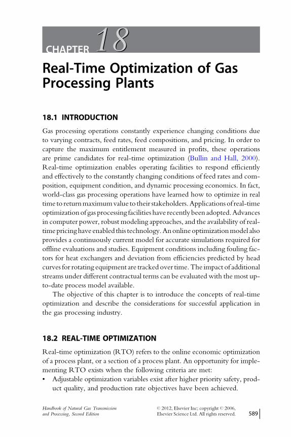
Figure 18-4 Real-time optimization RTS interface.


that would be difficult or impossible to solve using sequential techniques

offered by many flow sheet vendors.

A real-time optimization system will determine the plant optimum

operation in terms of a set of optimized setpoints. These will then be imple-

mented via the control system.

18.2.1 Physical PropertiesAll of the process models for a rigorous real-time optimization system use a

mixture of physical properties, such as enthalpy, K values, compressibility,

vapor pressure, and entropy. Equations of state, such as Soave–Redlich–

Kwong (SRK) or Peng–Robinson (PR), are used for fugacities, enthalpy,

entropy, and compressibility of the hydrocarbon streams. The enthalpy da-

tum is based onmethods such as the enthalpy of formation from the elements

at absolute zero temperature. This allows the enthalpy routines to calculate

heats of reaction as well as sensible heat changes. Steam and water properties

are calculated using routines based on standards such as theNational Institute

of Standards and Technology.


18.2.2 Optimization ModelsModels used in the optimization system must be robust, must be easily spec-

ified (in an automated manner) to represent changing plant situations, and

must solve efficiently. These models must be able to fit observed operating

conditions, have sufficient fidelity to predict the interactions among indepen-

dent and dependent variables, and represent operating limits or constraints.

State-of-the-art models meet these requirements by using residual format

(0¼ f(x)), open equations, fundamental,mechanistic relationships, andby in-

corporatingmeaningful parameterswithin themodels. These state-of-the-art

systems provide the highly efficient equation solver/optimizer and the inter-

face functionality that automates sensing the plant’s operating conditions and

situations, and they automate posing and solving the appropriate parameter

and optimization cases.

Most plant models are standard models. Sometimes custom models

are created specifically for the equipment of a unit. All the models use ther-

modynamic property routines for enthalpy, vapor-liquid equilibrium, and

entropy information.

Rotating equipment models such as compressor, pump, engine, gas tur-

bine, and steam turbine models contain, along with all the thermodynamic

relationships, the expected performance relationships for the specific equip-

ment modeled.

18.2.2.1 Optimization Objective FunctionThe objective function maximized by a high-level optimization system is

the net plant profit. This is calculated as product values minus feed costs

minus utility costs, i.e., the P – F –U form.When appropriately constrained,

this objective function solves either the “maximize profit” or “minimize

operating cost” optimization problem. Economic values are required for

each of the products, feeds, and utilities. The value of each stream is derived

from the composition-weighted sum of its components. Economic values

for feeds, products, and utilities in the optimization system are reset on a

regular basis for best performance.

18.2.2.2 Custom ModelsOften custom models must be incorporated into a standard optimization

package to predict proprietary processes and solvents. The custom model

may be incorporated with special properties packages or integrated into

the system in a semi-open approach where the iteration criterion is handled

by the optimization system, but the actual kinetics or thermodynamic


equations remain the same as the offline custom model. Proprietary gas

sweetening solvent formulations may be the most common example of a

custom model in the natural gas industry.

18.2.2.3 FractionatorsFractionators are modeled using tray-to-tray distillation. Heating and cool-

ing effects as well as product qualities are considered. Column pressure is

typically a key optimization parameter. Temperature measurements are used

to determine heat transfer coefficients for condensers and reboilers.

18.2.2.4 Absorbers and StrippersAbsorber and stripper units will be modeled using tray-to-tray distillation, if

required. Component splitters may be used to simplify the flow sheet where

acceptable when these units have little effect on the optimum.

18.2.2.5 Compression ModelThe main optimization setpoint variables for the compressors are typically

suction or discharge pressures. Important capacity constraints are maximum

and minimum speed for the driver; maximum current for electric motors;

and maximum power for steam turbines, gas turbines, and engines. Some-

times maximum torque will be considered for engines.

A multistage compressor model consists of models for a series of com-

pressor stages, interstage coolers, and adiabatic flashes. Drivers are included

for each compressor machine. For each single compressor stage, the inlet

charge gas conditions (pressure, temperature, flow rate, and composition)

and the discharge pressure specification are used with the manufacturer’s

compressor performance curves to predict the outlet temperature and com-

pressor speed. The power required for the compression is calculated from

the inlet and outlet conditions.

The first step in the development of the compression model is to fit the

manufacturer’s performance curves for polytropic head and efficiency to

polynomials in suction volume and speed.The equations for each compressor

stage (or wheel, if wheel information is available) take the following form:

Ep ¼ A �N2 þ B �N þ C �N � Vs þD � Vs þ E � Vs2 þ F (18-1)

Wp ¼ a �N 2 þ b �N þ c �N � Vs þ d � Vs þ e � Vs2 þ f (18-2)

where Vs is suction volume flow rate; N is compressor speed; Ep is stage or

wheel polytropic efficiency; Wp is stage or wheel polytropic head; and A

through F and a through f are correlation constants.


The polytropic head change across the stage or wheel can also be calcu-

lated from the integral of VdP from suction pressure to discharge pressure.

This integration can be performed by substituting V¼Z�R�T/P and inte-

grating by finite difference approximation:

Wp ¼ R � lnðPd=PsÞ � ððZs � TsÞ þ ðZd � TdÞÞ=2 (18-3)

where R is gas constant; Pd is discharge pressure; Ps is suction pressure; Zs is

compressibility at suction conditions; Ts is absolute suction temperature; Zd

is compressibility at discharge conditions; and Td is absolute discharge

temperature.

For simplicity, the preceding equations are formulated in terms of a sin-

gle integration step between suction and discharge, but in the actual imple-

mentation, each stage or wheel is to be divided into at least five sections to

describe the true profile. The enthalpy change across the stage or wheel can

be calculated from the inlet and outlet conditions, the polytropic head

change, and the polytropic efficiency.

This analysis results in three simultaneous equations and three unknowns

for each integration step. The unknowns are the discharge temperature, dis-

charge pressure, and enthalpy change for each step except the last. The known

dischargepressure for the last step is related to the speedof themachine. In state-

of-the-art approaches, all of the integration steps are solved simultaneously.

Measured discharge pressures, speeds, and temperatures are used in the

parameter estimation run to update the intercept terms in the polynomials

used to represent the manufacturer’s polytropic head and efficiency curves.

These parameters represent the differences between the actual performance

and expected/design performance. As compressors foul, these parameters

show increasing deviation from expected performance. It is this difference that

has significant meaning since an absolute calculation of efficiency at any

moment in time can vary with feed rate and several other factors, which dilute

the meaning of the value. By showing a difference from design, we get a true

measure of the equipment performance and how it degrades over time.

The discharge flow from each stage is sent through a heat exchanger

model coupled with an adiabatic flash. The heat transfer coefficient for each

exchanger is based on the measured suction temperature to the next stage,

corrected for addition of any recycle streams. Suction and/or discharge flows

are measured to fit heat loss terms in the interstage flash drums.

18.2.2.6 Distillation CalculationsStandard tray-to-tray distillation models are used for distillation calculations in

anoptimizationsystem.The“actual”numberof trays isusedwhereverpossible,


and performance is adjusted via efficiency. This allows the model to more ac-

curately represent the plant in a way that is understandable to a plant operator.

All distillation models predict column-loading constraints accurately as

targets are changed. Condenser and reboiler duties are also calculated for

predicting utility requirements and exchanger limitations.

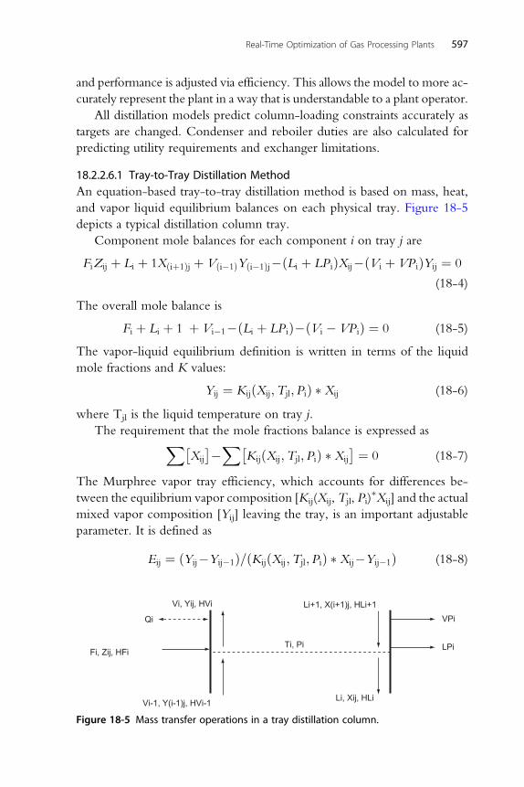
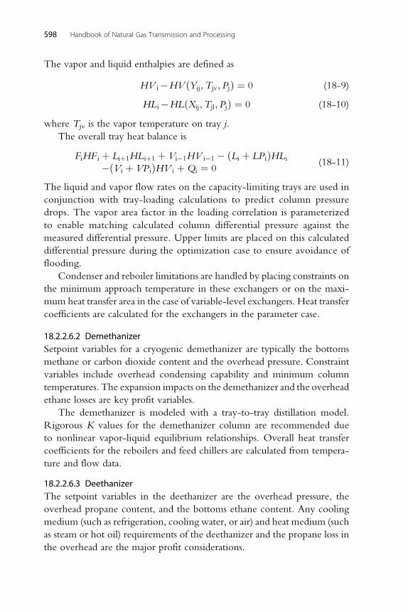
18.2.2.6.1 Tray-to-Tray Distillation MethodAn equation-based tray-to-tray distillation method is based on mass, heat,

and vapor liquid equilibrium balances on each physical tray. Figure 18-5

depicts a typical distillation column tray.

Component mole balances for each component i on tray j are

FiZij þ Li þ 1Xðiþ1Þj þ Vði�1ÞYði�1Þj�ðLi þ LPiÞXij�ðVi þ VP iÞYij ¼ 0

(18-4)

The overall mole balance is

Fi þ Li þ 1 þ Vi�1�ðLi þ LPiÞ�ðVi � VPiÞ ¼ 0 (18-5)

The vapor-liquid equilibrium definition is written in terms of the liquid

mole fractions and K values:

Yij ¼ KijðXij;Tjl;PiÞ � Xij (18-6)

where Tjl is the liquid temperature on tray j.

The requirement that the mole fractions balance is expressed asX

Xij

� ��X

KijðXij;Tjl; PiÞ � Xij

� � ¼ 0 (18-7)

The Murphree vapor tray efficiency, which accounts for differences be-

tween the equilibrium vapor composition [Kij(Xij, Tjl, Pi)�Xij] and the actual

mixed vapor composition [Yij] leaving the tray, is an important adjustable

parameter. It is defined as

Eij ¼ ðYij�Yij�1Þ=ðKijðXij;Tjl;PiÞ � Xij�Yij�1Þ (18-8)

Qi

Fi, Zij, HFi

Vi-1, Y(i-1)j, HVi-1

Vi, Yij, HVi

Ti, Pi

VPi

LPi

Li, Xij, HLi

Li+1, X(i+1)j, HLi+1

Figure 18-5 Mass transfer operations in a tray distillation column.


The vapor and liquid enthalpies are defined as

HV i�HV ðYij;Tjv; PjÞ ¼ 0 (18-9)

HLi�HLðXij;Tjl;PjÞ ¼ 0 (18-10)

where Tjv is the vapor temperature on tray j.

The overall tray heat balance is

FiHF i þ Liþ1HLiþ1 þ Vi�1HV i�1 � ðLi þ LPiÞHLi

�ðVi þ VPiÞHV i þQi ¼ 0(18-11)

The liquid and vapor flow rates on the capacity-limiting trays are used in

conjunction with tray-loading calculations to predict column pressure

drops. The vapor area factor in the loading correlation is parameterized

to enable matching calculated column differential pressure against the

measured differential pressure. Upper limits are placed on this calculated

differential pressure during the optimization case to ensure avoidance of

flooding.

Condenser and reboiler limitations are handled by placing constraints on

the minimum approach temperature in these exchangers or on the maxi-

mum heat transfer area in the case of variable-level exchangers. Heat transfer

coefficients are calculated for the exchangers in the parameter case.

18.2.2.6.2 DemethanizerSetpoint variables for a cryogenic demethanizer are typically the bottoms

methane or carbon dioxide content and the overhead pressure. Constraint

variables include overhead condensing capability and minimum column

temperatures. The expansion impacts on the demethanizer and the overhead

ethane losses are key profit variables.

The demethanizer is modeled with a tray-to-tray distillation model.

Rigorous K values for the demethanizer column are recommended due

to nonlinear vapor-liquid equilibrium relationships. Overall heat transfer

coefficients for the reboilers and feed chillers are calculated from tempera-

ture and flow data.

18.2.2.6.3 DeethanizerThe setpoint variables in the deethanizer are the overhead pressure, the

overhead propane content, and the bottoms ethane content. Any cooling

medium (such as refrigeration, cooling water, or air) and heat medium (such

as steam or hot oil) requirements of the deethanizer and the propane loss in

the overhead are the major profit considerations.


The deethanizer is modeled with a tray-to-tray distillation model.

Parameters include column pressure, column pressure drop, propane con-

tent in the deethanizer overhead, reflux flows, deethanizer bottoms ethane

content, and bottoms draw rate. Overall heat transfer coefficients are calcu-

lated for the exchangers.

18.2.2.6.4 DepropanizerThe setpoint variables for the depropanizer are the overhead butane content

and column pressure. Key constraint variables are the propane in the debu-

tanizer overhead, the overhead exchanger capacities, and column pressure

drop (flooding). Any cooling and heat medium usage requirements of the

depropanizer are the major profit considerations.

The depropanizer is modeled with tray-to-tray distillation models.

Parameters considered include column feed temperature, column pressure,

column pressure drop, butane content in the tops, reflux flow, bottoms pro-

pane content, and bottoms draw rate. Overall heat transfer coefficients are

calculated for the reboiler and condenser. A column capacity factor is also

parameterized.

18.2.2.6.5 DebutanizerThe setpoint variables for the debutanizer are the overhead pentanes and

heavier content as well as column pressure. Key constraint variables are

the propane in the debutanizer overhead, the overhead exchanger capacities,

and column pressure drop (flooding). Any heating and cooling medium us-

age requirements of the debutanizer are the major profit considerations.

The debutanizer is modeled with a tray-to-tray distillation model. Pa-

rameters considered include column feed temperature, column pressure,

column pressure drop, pentanes and heavier content in the overhead, reflux

flow, bottoms butanes content, and bottoms draw rate. Overall heat transfer

coefficients are calculated for the reboiler and condenser. A column capacity

factor is also parameterized.

18.2.2.6.6 Butanes SplitterThe setpoint variables for the butanes splitter are the column pressure, nor-

mal butane in overhead, and isobutane in the bottoms. The constraint

variables of interest are reboiler and condenser loading and product specifi-

cations. The profit variables of interest are the isobutane losses in the bottoms

normal butane stream.

The butanes splitter is modeled with a tray-to-tray distillation model.

The parameters considered include column pressure, column differential


pressure, normal butane in the isobutane product, bottoms isobutane

concentration, reflux flow rate, bottoms flow rate, product draws, and bot-

tom reboiler flow rate. Heat transfer coefficients for the exchangers are

calculated.

18.2.2.6.7 Refrigeration ModelsThe main setpoint variable for refrigeration machines is the first-stage suc-

tion pressure. Refrigeration system models relate refrigeration heat loads to

compressor power. The compressor portions of the refrigeration models use

the same basic equations as compressor models discussed previously. Refrig-

eration systems should use the appropriate composition and will have a com-

ponent mixture for any makeup gas.

The measured compressor suction flows and the heat exchange duties

calculated by the individual unit models are used to determine the total re-

frigeration loads. The refrigerant vapor flows generated by these loads are

calculated based on the enthalpy difference between each refrigerant level.

Exchanger models of the refrigerant condensers are used to predict compres-

sor discharge pressures.

18.2.2.6.8 Demethanizer Feed Chilling ModelsThe demethanizer feed chilling system is modeled as a network of heat

exchangers and flash drums. These models are used to predict the flow rates

and compositions of the demethanizer feeds. The effects of changing

demethanizer system pressures and flow rates are predicted.

The demethanizer feed drum temperatures and feed flow rates are mea-

sured to fit the fractions of heat removed from the feed gas by each

exchanger section. Flow and temperature measurements on the cold stream

side allow the fraction of feed gas heat rejected to each stream to be esti-

mated. The two sides of the feed exchangers are coupled through an overall

heat balance. The inlet and outlet temperatures from the refrigerant and

other process exchangers are used to fit overall heat transfer factors in the

parameter case. A pressure drop model for the feed gas path is also included.

18.2.2.7 Steam and Cooling Water System ModelsHeat and material balance models of the steam system are developed. These

models include detailed representations of the boilers.

The cooling water systemwill be modeled with heat exchangers, mixers,

and splitters to allow for constraining the cooling water temperature and its

effects on the operation of distillation columns and compressors.


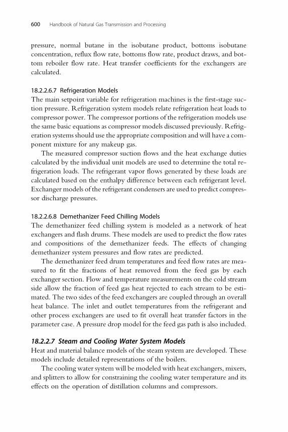
18.2.2.8 TurbinesA turbine model, as shown in Figure 18-6, is used for steam turbines (back

pressure, condensing, or extraction/condensing) or any expander in which

the performance relationship can be expressed using the following equation:

Design Power ¼ Aþ B� ðMass FlowÞ þ C� ðMass FlowÞ2 þD

� ðMass FlowÞ3(18-12)

Back pressure and condensing turbine expected performances are usually

presented as essentially linear relationships between power and steam flow.

Extracting/condensing turbine expected performance relationships are typ-

ically presented as power versus throttle steam flow, at various extraction

steam flows. This kind of performance “map” can be separated into two

relationships of the aforementioned form: one representing the extraction

section, and the other the condensing section. An extraction/condensing

turbine can be thought of as two turbines in series, with part of the extraction

section flow going to the condensing section.

Design power refers to expected power from performance “maps” that

are at specific design inlet pressure, inlet temperature, and exhaust pressure.

Expected power is the power expected from a turbine operating at other

than design conditions. The design power is adjusted by the “power factor,”

as illustrated here:

Expected Power ¼ Design Power � Power Factor (18-13)

Inlet(Throttle)

1

Gland Losses

Power Losses

2

Outlet(Exhaust)

Power

Figure 18-6 Schematic of turbine model.


Power Factor ¼ DIsentropic Enthalpy at actual conditions

DIsentropic Enthalpy at design conditions(18-14)

BrakeðshaftÞPower ¼ Expected Power þ Power Bias (18-15)

Design power and expected power are equal if actual expanding fluid (i.e.,

steam) conditions are the same as design conditions. The power bias can be

parameterized using the exhaust temperature for back pressure turbines or

the extraction section of an extraction/condensing turbine. In both of these

cases, the exhaust steam is superheated (single phase). For condensing tur-

bines or the condensing section of an extraction/condensing turbine, the

measured steam flow is calculated because the temperature of the two-phase

exhaust cannot be used. The fraction vapor of the two-phase exhaust is de-

termined by energy balance. The total energy demand can be determined

from the compressor (or other driven power consumer). The power

extracted from the extraction section can be determined from the throttle

steam flow and the inlet and outlet (single-phase) conditions. The power

extracted from the condensing section is just the difference between the total

demand and the extraction section power.

The power loss is taken from the steam and affects its outlet conditions

but is not transferred to the shaft or brake power.

To calculate the change of enthalpies needed for the power factor and for

the energy balance, we calculate fluid conditions for each turbine section at

the inlet (throttle), outlet (exhaust), and at inlet entropy and outlet pressure

for both actual and design conditions. The nomenclature associated with the

exhaust fluid conditions required for the enthalpy change calculations is

Exh IDM¼Exhaust Isentropic at Design inlet conditions for vapor/

liquid Mixture

Exh IDV¼Exhaust Isentropic at Design inlet conditions for Vapor

Exh IDL¼Exhaust Isentropic at Design inlet conditions for Liquid

Exh IAM¼Exhaust Isentropic at Actual inlet conditions for vapor/

liquid Mixture

Exh IAV¼Exhaust Isentropic at Actual inlet conditions for Vapor

Exh IAL¼Exhaust Isentropic at Actual inlet conditions for Liquid

For condensing turbines or the condensing section of extraction/condens-

ing turbines, the exhaust pressure is used to specify the model. The parameter

that this measurement updates is the condenser heat transfer coefficient.

The exhaust pressure is free to move in the optimization cases, since the actual

pressure moves as the condenser calculates the pressure required to condense

the steam sent to the condensing turbine or condensing section.


The maximum mass flow at reference (usually design) conditions is used

to predict the maximum mass flow at actual conditions as an additional con-

straint on the turbine performance. Sonic flow relationships are used for this

prediction. This is the maximum flow through the inlet nozzles when the

inlet steam chest valves are wide open. The nozzle area is not needed if

the maximum flow at a set of reference conditions is known. Vendors usu-

ally list the maximum flow, not the nozzle area.

The model also includes the gland steam flow, which is used to counter-

balance the axial thrust on the turbine shaft and which is lost through lab-

yrinth seals. The gland steam does not contribute to the shaft power.

Typically, turbine performance is not considered to be a function of

speed. Consequently, speed is a variable that has no effect on the solution.

However, turbine performance is typically a very weak function of speed

over a wide range, and its effect on performance is not typically presented

on the expected performance “maps.” The possibility of adding the weak

effect of speed on performance will be considered when the model is being

built.

18.2.3 Plant Model IntegrationAfter the plant section models have been developed, they are integrated into

the overall plant model. All of the interconnecting streams are specified

and checked, and a consistent set of variable specifications is developed. At this

stage, the overall validity of the plant model is checked using offline plant data.

Reconciliation/parameter and optimization cases are run, and the results

are checked for accuracy and reasonableness. A material balance model is

included in the plant model integration work to confirm an absolute model

material balance closure. This material balance will include a furnace area

balance, a recovery area balance, and an overall balance. In addition, the

plant integration allows the objective function to be tested and validated

with connections to all feed, product, and utility variables.

It is important to have the engineers that will be responsible for commis-

sioning the optimization system involved in the project during plant model

integration. A thorough understanding of the plant model is imperative for a

smooth implementation of the online system.

18.2.3.1 Model Fidelity and Measurement ErrorsIn an optimization system as described here, neither the models nor the mea-

surements need to be absolutely perfect for the system to work well and to

deliver significant improvement in profitability. An online optimization


system continuously receives feedback from real-time measurements. The

model parameters are updated prior to each optimization so that the models

fit the plant and the optimum setpoints calculated are valid and can be

confidently implemented. Without this constant feedback of plant measure-

ments and regular updating of the plant model, the optimization solution

might not be feasible. The fidelity of the models and the accuracy of the

measurements are reflected in trends of the parameters. During commission-

ing of the optimization system, the best available measurements are identi-

fied by analyzing many parameter cases, running with real-time data, and

prior to closing the loop.

If, for example, significant heat balance discrepancies exist between pro-

cess side and fuel/flue gas side measurements in a furnace, that discrepancy

can be handled by determining the bias required on the fuel gas flow mea-

surement(s) to satisfy the heat balance. That bias could be a parameter that is

updated prior to each optimization. The variation of the bias over time (its

trend) would be monitored. If this parameter varies significantly, the furnace

model and other measurements used by it would be investigated thoroughly.

Alternate measurements used to “drive” the parameter case solution would

be investigated as well. The outcome of this analysis is that the best available

measurements are selected, and the model relationships are thoroughly in-

vestigated to ensure that all significant relationships are included. This anal-

ysis is a standard and required step in building the optimization system.

Validity checking is an integral part and is built into an online optimiza-

tion system. It is used to screen out gross errors. If alternate measurements are

available, the validity checkers can use these when primary measurements

are unavailable or bad. Generic validity checking takes care of common er-

rors, while custom validity checking can respond to site-specific situations.

Measurements can be designated as critical, so if they are unavailable, the

optimization cycle will be directed to monitor for steady state and will com-

plete its cycle only when the measurement becomes available. Validity

checking has several features designed to keep the online service factor

of the optimization system high in the face of imperfect measurements.

Another feature of the online system is that the measurements used to drive

the solution of the parameter case are averages over a specified time window

(usually 1 hour) so that measurement noise is suppressed.

The better the measurements and the better the models, the better a real-

time optimization can fully exploit the process equipment, and conse-

quently, the more potential profit is realized.

Processing RTO in the future will likely include wider applications

driven by demonstrated benefits, reduced implementation costs, and


acceptance as a best practice. RTO applications are also becoming tightly

intertwined with economic planning systems, where real-time pricing

and contractual considerations are available.

Evolving technologies changing the value proposition for refining RTO

include

• Detailed kinetic models for all major processing units and configurations,

proven by reported applications.

• Optimization technology improvements that incorporate robust solvers,

integer variables, and the capability to handle increasing problem sizes.

Today’s technology can handle applications with several hundred thou-

sand equations; a typical refining application has 100 measurements,

more than 100,000 variables, and 25 outputs.

• Greater integration with higher-level systems including shared models

and reconciled measurement data.

• Multiunit optimization that leverages shared resources between process

units and continues to lead toward rigorous refinerywide optimization.

• Computing technology improvements, which have already shiftedRTO

from minicomputers to personal computers, and which will allow more

solutions per day andmore complex formulations. Solver and computing

improvements will eventually lead to true dynamic optimization.

• Application and model building tools, operating graphical user inter-

faces, and sustained performance technologies that will lower cost, im-

prove benefits, and remove other hurdles.

18.3 REAL-TIME OPTIMIZATION PROJECT CONSIDERATIONS

The steps of a real-time project implementation include

• Front-end engineering design

• Flow sheet development

• Model testing and tuning

• Online open loop testing

• Online closed loop testing

• Application sustainment

During front-end design, the project objectives should be clearly de-

fined, including

• Process envelope: The system boundaries need to be determined,

including the process equipment included within the boundary.

Various equipment lineups that will be considered for optimization

are identified. Also, the modeling methodology decisions occur at

this stage.


• Economic parameters and objective function: The profit function

requires definition, including the specific economic parameters that

contribute to the profit function.

• Source of process and economic information: Process and economic

information will be available from various sources. Process information

is typically acquired from a process historian, whereas economic infor-

mation will come from various commercial sources. Care should be

taken to determine a source that is current and updated frequently.

• Setpoints to be generated from the optimizer: Process setpoints are critical

for effective optimization. These setpoints must be selected where process

control action will be attained accurately. Advanced process control strat-

egies are usually best for implementing setpoints from a real-time analyzer.

• Metrics required for success: Metrics to track optimizer online time as

well as optimizer effectiveness should be determined. An owner of these

metrics should be identified to take responsibility for the success and sus-

tainability of the optimizer.

Flow sheet development is obviously a critical step in the implementa-

tion of a real-time optimization project. The flow sheet should be developed

by subsections of the plant and imported into the main application flow sheet

as block diagrams. Redundant streams and equipment used in the initializa-

tion phase are removed from the flow sheet, and the sections of the plant are

connected together at the block boundaries to fully integrate the subsections

into a single flow sheet. Unit and flow sheet customizations are then added

to improve the model’s representation of the process.

Model testing and tuning include reconciling the imported data in offline

mode and testing the real-time sequencing. The standard data reconciliation

report is used to identify themeasurements with theworst mismatch, and cor-

rective action is taken. The model is then tested by importing multiple sets

of data via the electronic data interface before placing the model online.

Optimization cases are run and verified. Steady-state detection is fine-tuned.

Initial online runs are observed to verify transfer of optimal setpoints to the

advanced control and distributed control systems.

Sustainment of the application is critical to the long-term success. An

engineer should be assigned responsibility for maintaining the application and

working with operations to resolve any concerns immediately. Metrics should

be tracked and reported to measure the success. These metrics may include

• The time on optimization as a percentage of time on control, averaged

over all optimizable controllers.

• The time the optimizable controllers had optimization setpoints rejected

as a percentage of the time on control.


• The time the optimizable controllers ran at expired optimization set-

points as a percentage of the time on control.

Optimization setpoints should expire after a predetermined amount of

time, reflecting the nominal period for which a single optimization solution

is valid. A standard stream-factor tracking program will calculate and report

these statistics.

18.4 EXAMPLE OF REAL-TIME OPTIMIZATION

The Gassled joint venture operated by Gassco and supported by Statoil ap-

plied real-time optimization at their Karst� gas processing plant in Norway

(Kovach et al., 2010). Themodel is called the Plant Production Performance

Model (3PM).

Karst� is the largest natural gas liquids (NGL) plant in Europe. The

Gassled owners have first rights to book capacity. Spare capacity is available

for any other qualified shipper and subject to published tariffs for transport-

ing and processing gas.

Gassled has a flexible gathering network connecting the respective pro-

ducers and processing terminals, allowing gas streams from several fields to

be routed todifferentdestinations.Mixingofgas streamsprovides sales gasqual-

ity with respect to gross calorific value (GCV), Wobbe index (WI), and CO2.

Rich gas processing capacity at the Karst� plant depends on several vari-

ables and constraints. One of the most significant variables is the feed gas

composition. Simulations demonstrate that the rich gas processing capacity

may be significantly lower than the nominal design capacity if the feed has a

high NGL content.

New expansion to increase the capacity of the Karst� facilities has

increased the complexity of the Karst� facilities. The need for an onlinemodel

to determine plant capacity was recognized to enable the plant to operate

with a high degree of capacity utilization, realizing that production regular-

ity is an inherent property of the throughput obligations. Underutilization of

capacity sacrifices processing fees. The real-time optimization model allows

precise and reliable capacity predictions while reducing the work required to

determine the capacity. Operating setpoints required to reach the predicted

capacity are generated as well as information for maintenance planning and

infrastructure development.

18.4.1 Process DescriptionFigure 18-7 shows a simplified process diagram of the Karst� gas processingplant. As can be seen, rich gas enters the plant and is preconditioned by

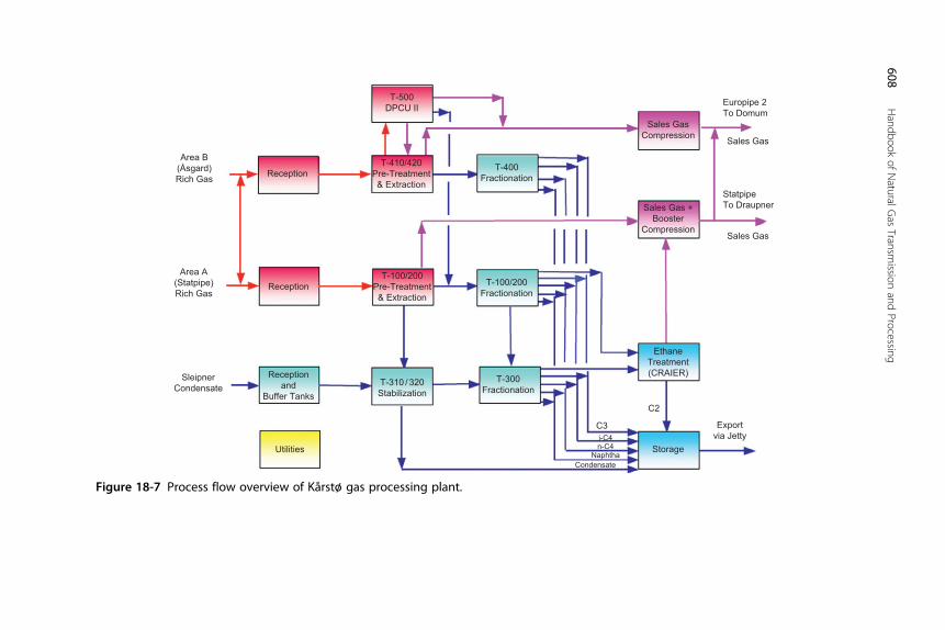
Area B(Åsgard)Rich Gas Reception

T-500DPCU II

T-400Fractionation

Sales GasCompression

Sales Gas +Booster

CompressionSales Gas

EthaneTreatment(CRAIER)

C2

Exportvia Jetty

Storage

C3

T-300Fractionation

T-310 / 320Stabilization

Receptionand

Buffer Tanks

Utilities

SleipnerCondensate

Area A(Statpipe)Rich Gas

ReceptionT-100/200

Pre-Treatment& Extraction

T-100/200Fractionation

i-C4n-C4

NaphthaCondensate

Sales Gas

StatpipeTo Draupner

Europipe 2To Domum

T-410/420Pre-Treatment& Extraction

Figure 18-7 Process flow overview of Kårsto/ gas processing plant.

608Handbook

ofNaturalG

asTransm

issionand

Processing


removal of H2S and mercury. The gas is then preheated prior to dehydra-

tion, andNGL is extracted from the rich gas. The fractionation facilities pro-

duce raw ethane, stabilized condensate, propane, n-butane, i-butane, and

naphtha. CO2-rich ethane extracted from each train is routed for purifica-

tion of ethane.

The processing facilities include 26 distillation columns. Steam is used as

the heating medium for the reboilers on the distillation columns and to

power turbines. Steam boilers and waste heat recovery systems on gas tur-

bines generate the steam. Three levels of steam are employed. Additional

utilities used are sea water for cooling and propane for refrigeration.

Sales gas is exported to two high-pressure subsea pipelines operated

at pressures up to 189 barg. The export compression facilities include

four compressor manifolds operated at different suction and discharge

pressures. The compressors are driven by both gas turbines and electric

motors.

In the Karst� plant, the extraction trains may be bypassed. This allows

more gas to be produced and processed. However, the bypass quantities

are limited to provide sales gas quality to comply with the GCV, WI, and

CO2 specifications.

18.4.2 Plant OperationEffective field production and development of new offshore fields require

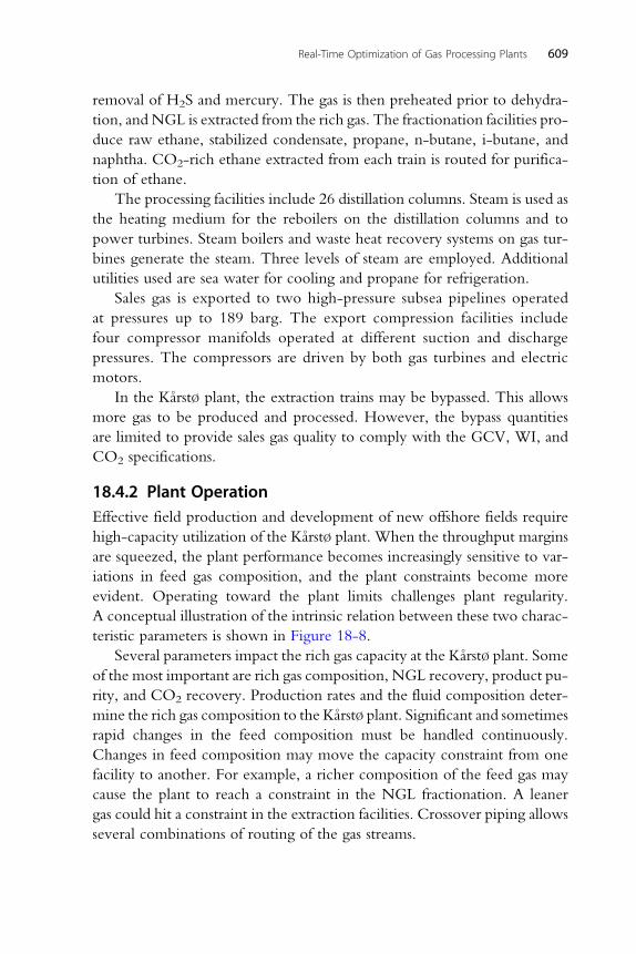
high-capacity utilization of the Karst� plant. When the throughput margins

are squeezed, the plant performance becomes increasingly sensitive to var-

iations in feed gas composition, and the plant constraints become more

evident. Operating toward the plant limits challenges plant regularity.

A conceptual illustration of the intrinsic relation between these two charac-

teristic parameters is shown in Figure 18-8.

Several parameters impact the rich gas capacity at the Karst� plant. Some

of the most important are rich gas composition, NGL recovery, product pu-

rity, and CO2 recovery. Production rates and the fluid composition deter-

mine the rich gas composition to the Karst� plant. Significant and sometimes

rapid changes in the feed composition must be handled continuously.

Changes in feed composition may move the capacity constraint from one

facility to another. For example, a richer composition of the feed gas may

cause the plant to reach a constraint in the NGL fractionation. A leaner

gas could hit a constraint in the extraction facilities. Crossover piping allows

several combinations of routing of the gas streams.

100 %P

lant

Reg

ular

ity

Capacity Utilization 100%

IncreasedCapacityUtilization

Enhancementwith 3PM

Figure 18-8 Trade-off between plant regularity and capacity utilization (Kovachet al., 2010).


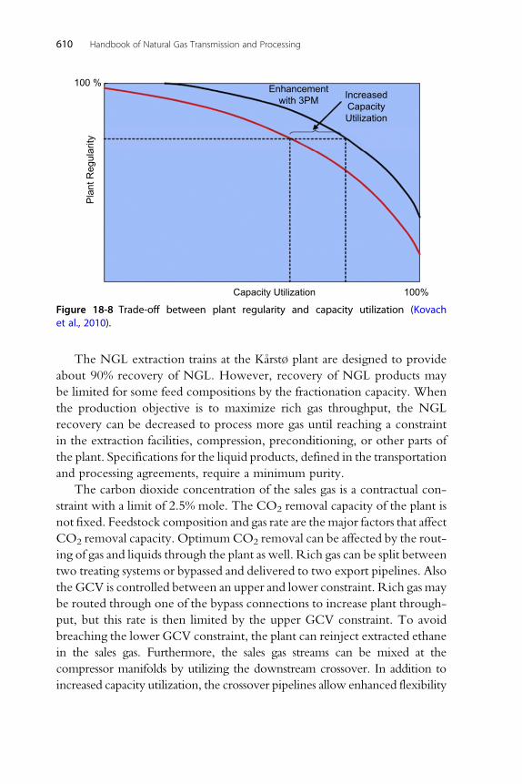
The NGL extraction trains at the Karst� plant are designed to provide

about 90% recovery of NGL. However, recovery of NGL products may

be limited for some feed compositions by the fractionation capacity. When

the production objective is to maximize rich gas throughput, the NGL

recovery can be decreased to process more gas until reaching a constraint

in the extraction facilities, compression, preconditioning, or other parts of

the plant. Specifications for the liquid products, defined in the transportation

and processing agreements, require a minimum purity.

The carbon dioxide concentration of the sales gas is a contractual con-

straint with a limit of 2.5% mole. The CO2 removal capacity of the plant is

not fixed. Feedstock composition and gas rate are the major factors that affect

CO2 removal capacity. OptimumCO2 removal can be affected by the rout-

ing of gas and liquids through the plant as well. Rich gas can be split between

two treating systems or bypassed and delivered to two export pipelines. Also

the GCV is controlled between an upper and lower constraint. Rich gas may

be routed through one of the bypass connections to increase plant through-

put, but this rate is then limited by the upper GCV constraint. To avoid

breaching the lower GCV constraint, the plant can reinject extracted ethane

in the sales gas. Furthermore, the sales gas streams can be mixed at the

compressor manifolds by utilizing the downstream crossover. In addition to

increased capacity utilization, the crossover pipelines allow enhanced flexibility


of the operations with respect to handling of feedstock variations. It is possible

to mix the various feed streams to optimize NGL recovery, CO2 extraction,

and quality of the products.

18.4.3 Production ObjectivesThe primary production objective is typically plant throughput and to de-

liver sales gas and products within the specifications. However, the produc-

tion objectives include maximum daily throughput, high annual capacity

utilization, optimumNGL production, and optimum fuel gas consumption.

Most shippers request high production at Karst� throughout the year,

taking into account the seasonal swing in gas demand. This means high de-

mand for processing capacity at Karst� throughout the year.

The operator is responsible for coordination of the yearly maintenance

planning of all the installations connected to the gas transport infrastructure.

A primary objective is to obtain a total plan where the availability of gas for

deliveries to the market is maximized. Depending on the extent of yearly

maintenance at Karst� as well as at the upstream fields, this could put restric-

tions on production from certain fields, or allow accelerated production of

more NGL rich or CO2 rich gas from other fields. Maximizing CO2 pro-

duction fromCO2 rich fields could imply postponed or reduced investments

in future CO2 removal capacity to meet sales specifications.

In periods when processing demand is below the plant capacity (when

Karst� has no bottleneck effect on the offshore production), the primary op-

erational objective is to maximize NGL recovery in order to provide for in-

creased value creation for the shippers. For the NGL products, this means

achieving the minimum product purity.

The Karst� plant is a large energy consumer, and optimizing energy con-

sumption is an important objective. However, optimizing energy consump-

tion should not compromise the primary production objectives, related to

the value creation at Karst�.

18.4.4 Project DriversValue generated by real-time optimization for the Karst� plant operations

comes from the following:

• Increased utilization of the plant capacity, by introducing real-time

optimization

• Improved quality of the capacity figures issued for booking


• Reduced time needed to prepare for the booking process

• Improved position in the business development process

On a daily basis, the feed stream compositions will vary. Processing feeds

of variable composition require the plant control system to give fast and ac-

curate responses, in order to maintain production targets. Skilled operators

have a basic understanding of the plant operational characteristics and learn

how to respond to feed disturbances. However, in transition periods, the

plant capacity will not be fully utilized. Also, the operators may not push

the plant to its full capacity, or they may choose a suboptimal routing of

the gas through the processing facilities. On a regular basis, the real-time op-

timization determines optimized setpoints for the advanced control system,

thereby ensuring a rapid and smooth transition period to new optimal plant

conditions.

An illustration of the possible benefits with the 3PM employed for RTO

to handle feed composition variations is shown in Figure 18-9. In this ex-

ample, the primary operational objective is to achieve maximum plant

throughput. The upper curve illustrates achieved production over a day

when the operator employs the 3PM. The lower curve illustrates production

with no 3PM implemented. It should be recognized that the upper curve

assumes a shorter transition period following changes in the feed conditions.

The 3PM model enables an increase of the plant throughput by 1%.

Plant regularity has a very high focus, and a regularity target of at least

98.5% is set for the Karst� plant. However, when failure occurs, emphasis

is put on maintaining the highest possible service degree to limit upstream

consequences to oil production and minimize the consequences for the gas

Ric

h G

as P

rodu

ctio

n R

ate

Narrowing theTransitionPeriod

Enhancement with 3PM

WithoutEmploymentof 3PM

3PM CapacityImprovementTarget: 1%

Figure 18-9 Illustration of enhanced processing capabilities.


customers. In situations in which equipment exhibits underperformance

such as fouling in heat exchangers or degrading of compressors, this is

revealed by the optimization model, and appropriate actions to correct

the problem could be executed. If equipment fails to work or is temporarily

out of service, the optimization model automatically computes new set-

points of the advanced process control to minimize the consequences.

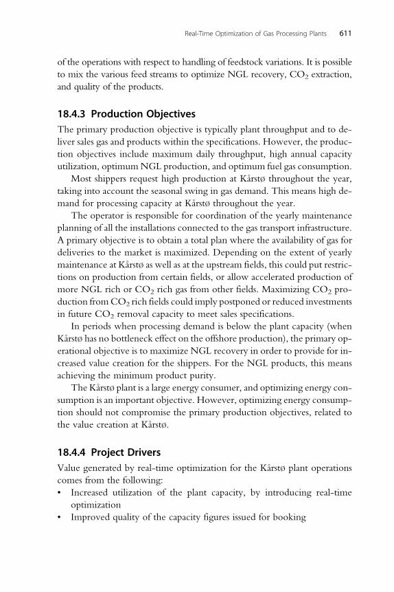
The operator of the plant is responsible for issuing capacity figures for the

booking processes. Often there are requests for processing capacity beyond

current capacity at the plant. This puts pressure on the capacity margins of

the plant. With the optimization model, which closely mimics the real op-

eration performance, Gassco can provide enhanced confidence to reduce the

uncertainty margins.

Extraction of NGL from the rich gas and subsequent fractionation into

commercial products adds value to the shippers. Some shippers limit their

gas deliveries based on their booked fractionation capacity, whereas shippers

with leaner gas are limited by their booked extraction capacity. Any free

processing capacity is identified and can be available to the shippers, allowing

them to optimize their petroleum portfolio. This allows accelerated produc-

tion of NGL-rich gas to maximize revenue for the shippers.

Boosting processing capacity within the limits of the facilities is the pri-

mary objective. The online model improves planning with a higher accuracy

than the current process simulation models. Improved quality and accuracy

of the planning tool results in a higher confidence in the calculation of

the maximum plant capacity, denoted available technical capacity (ATC).

The capacity committable on a long-term basis is denoted maximum avail-

able capacity (MAC). This allows for an operational margin for daily oper-

ations, as shown in Figure 18-10.

Reduced uncertainty due to the capability of the optimization model

may narrow the operational margin and thereby increase the MAC. The

biannual capacity estimation process is demanding and time consuming.

Performance of existing equipment and systems that limit capacity utiliza-

tion of the plant requires evaluation. The optimization model allows this

estimation process to be run more efficiently.

18.4.5 Features of the Optimization ModelA single model that is applied for various purposes minimizes the inconsis-

tency between various simulation results and the actual operation of the

plant. A high degree of confidence in the planning scenarios and simulation

results is achieved as the same model is applied for optimization of the plant

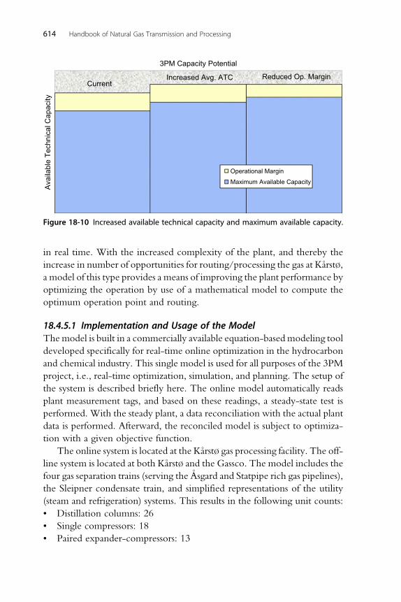
Operational Margin

Current

Ava

ilabl

e Te

chni

cal C

apac

ity

Increased Avg. ATC Reduced Op. Margin

3PM Capacity Potential

Maximum Available Capacity

Figure 18-10 Increased available technical capacity and maximum available capacity.


in real time. With the increased complexity of the plant, and thereby the

increase in number of opportunities for routing/processing the gas at Karst�,a model of this type provides a means of improving the plant performance by

optimizing the operation by use of a mathematical model to compute the

optimum operation point and routing.

18.4.5.1 Implementation and Usage of the ModelThemodel is built in a commercially available equation-basedmodeling tool

developed specifically for real-time online optimization in the hydrocarbon

and chemical industry. This single model is used for all purposes of the 3PM

project, i.e., real-time optimization, simulation, and planning. The setup of

the system is described briefly here. The online model automatically reads

plant measurement tags, and based on these readings, a steady-state test is

performed. With the steady plant, a data reconciliation with the actual plant

data is performed. Afterward, the reconciled model is subject to optimiza-

tion with a given objective function.

The online system is located at the Karst� gas processing facility. The off-line system is located at both Karst� and the Gassco. The model includes the

four gas separation trains (serving the Asgard and Statpipe rich gas pipelines),

the Sleipner condensate train, and simplified representations of the utility

(steam and refrigeration) systems. This results in the following unit counts:

• Distillation columns: 26

• Single compressors: 18

• Paired expander-compressors: 13


• Process measurements: 1600

• Controllers (regulatory and advanced control, 175 and 110 variables,

respectively)

• Associated heat exchangers, drums, motors, furnaces, pumps, pipes, and

valves

The output of the optimization is a set of setpoints to the advanced con-

trol system. The online model is anticipated to run in intervals of 2–4 hours,

depending on solution time, performance, and actual implementation and

usage in the daily routines.

The planning interface is a simplified representation of the plant in an

external graphical user interface (GUI), where one has the opportunity to

generate new feeds by mixing different field flows and compositions, to test

out the performance in simulation, as well as optimization mode. The sim-

plified representation of the plant consists in principle of a block diagram,

where the blocks represent sections of the plant. The planner then has

the option to switch off one or more blocks and check the capacity (perfor-

mance) of the plant with this very simplified model user interface. The fact

that the planner has a simplified overall GUI for the model of the plant, with

a number of sections representing logical groups of unit operations in the

plant, makes it easy to do scenario analysis for both new fields (new com-

positions) and for shutdown and maintenance. In each case, it becomes eas-

ier for the planning department to give a precise answer to the capacity of

any feed with a given layout of the plant.

Simulation is done in the core model GUI, which is also used in the

real-time optimization mode. Further, new plant developments may be

simulated with the model in order to get a better prediction of throughput

capacity than a conventional simulation would give.

The online model is located on a computer in the plant control room. It

is running in a fully automated fashion, on a given interval basis. The model

immediately sends the solution to a central storage computer. From here, the

model can then be accessed by planners and offline simulation engineers,

who copy the solved models to their own computers, respectively. This

facilitates a common arena for operations as well as the planning and engi-

neering departments.

The online model produces results to various types of end users. In ad-

dition to generating the actual setpoints to the advanced control system (and

the operators), the model generates a set of reports with different types of

information every time it is solved. The type of information to be generated

is mass and energy balances, production figures, economical performance,


utility consumption, capacity utilization of each unit, shadow prices, and

equipment monitoring.

18.4.5.2 Modeling and Optimization StrategyThe plantwide model for the Karst� plant comprises all processing facilities,

as well as the steam boilers and other utilities. The single plant model is based

on open equations. The individual unit operations are modeled by use of

standard library models. In the cases of rotating equipment and important

valves, Statoil and original vendor performance curves are used. The plant

instruments that the model reads and applies are carefully chosen, in order to

ensure that sufficient and trustworthy signals form the basis of the data rec-

onciliation and, subsequently, the optimization. All alternative operation

scenarios in terms of equipment failure, maintenance, etc., are dealt with

by lineups defined by a set of macros.

The various crossovers that are normally in use in the plant are treated as

continuous variables in order to avoid integer variables in the optimization

problem. Only equipment that plays an active role in the plant is modeled,

and the set of compounds used are as comprehensive as necessary to achieve

representative results. This is in order to maintain a fairly reasonable size (and

solution time) of the model.

The model (and the planning facility) comprises a set of objective func-

tions from which one can be applied according to the desired operation

mode. The objective functions for the optimizer reflect operation modes

that are, or may be, relevant to operation of the Karst� plant. The objectivefunctions are predefined and can be chosen arbitrarily by the system admin-

istrator. Typical examples of objective functions are to maximize sales gas

production or to maximize liquid NGL production. For all cases, the general

product qualities are modeled as constraints together with the relevant op-

erational limitations.

There are over 100 flags to indicate the routings and equipment status in

the plant. While the physical realities prevent this from being a true com-

binatorial problem, in practice there are easily over a hundred possible plant

configurations. This poses challenges in both making sure that the appropri-

ate equipment is on or off in the model, but more importantly, in creating a

good starting point for the equation-based solver.

In addition, the CO2 removal and ethane recovery unit can operate near

the CO2/C2 azeotrope, and some portions of the unit approach the critical

point of the mixture. As with most modern gas plants, it is heavily heat

integrated with many heat-pumped columns, cold boxes, and paired

expander-compressors.


18.4.5.3 Online UsageThe online system follows the sequence of detecting steady state, checking

data consistency, reconciling the data, calculating the optimal setpoints, and

sending the optimized setpoints to the controllers.

18.4.5.4 Quantifying Measurement ErrorsThe 3PM model imports over 1,600 process measurements, which are used

in data reconciliation. Of these, several hundred were identified as key pro-

cess variables and have results from the data reconciliation runs written back

to the database. The data exported for these points consist of the sample

value used in the data reconciliation, the reconciled value, and the measure-

ment offset.

Some nonmeasured variables such as compressor efficiencies are also

saved. The scan and reconciled values are accessible on operator process dis-

plays. The same operator displays have links to preconfigured trends of the

measurement offsets. This gives operations a quick way of evaluating the ac-

curacy of their process measurements and seeing inferred values (e.g., effi-

ciencies and unmeasured temperatures) in a familiar format.

Data reconciliation detects and runs when the plant is steady and puts the

data in a readable format that supports scanning the data over long time pe-

riods. Any trended offset that is not distributed around zero and that has a

consistent bias may be in error.

A suspected point can be immediately checked. Quantifying measure-

ment errors can also help improve the accuracy of other offline simulation

tools. Any process variable that is used as a specification in a process simulator

needs to be accurate. Detecting a bias can significantly improve the accuracy

of the simulation results.

In addition to highlighting possible measurement errors, an understand-

ing of the behavior of unmeasured variables such as intermediate tempera-

tures or efficiencies can have a positive impact on operations. Data

reconciliation results have highlighted differences in efficiencies between

parallel compressor trains and furnaces.

18.4.5.5 Offline UsageThe offline system consists of a web-based interface, a SQL data repository

for storing cases, and rigorously validated models from the online system.

The interface is designed to facilitate queued simulation and optimization

runs of the most common plant configurations using various combinations

of flows from the 30þ fields that feed the plant. Planning personnel have the

option to run the model either through the standard web-based simulation


interface or through the more detailed model builder interface. The latter is

used to explore special situations that are not supported by the web-based

interface. This requires a more detailed knowledge of the model and the

simulation software. The model is run in this mode only to conduct special

studies with high value.

18.4.5.6 Use for PlannersThe user of the planning system can use two strategies to create a starting

point. In the first, the user starts with an online model taken from the fully

operational plant and then specifies the sections that are to be turned off and

the feed rates. In the second, the user begins with an online model that very

closely resembles the plant configuration he wishes to model.

For general studies, the first method is simpler and will generate accept-

able results. For very specific conditions such as modeling CO2 constraints,

the secondmethod will generate the most accurate results because the model

tuning parameters will have been reconciled for the exact conditions of

interest.

The second method is feasible because the online system archives valid

models to a separate directory. In this way, a library of models for all process

operating modes is created automatically.

To locate the time of the desired operating mode, the user can either

look at trends of the appropriate equipment flags or use the operator display

to identify the time and date that the appropriate model was created. Once

the date is determined, the user can then copy themodel from the library and

move it into the planning system for further study.

18.5 REFERENCESBullin, K.A., Hall, K.R., 2000. Optimization of Natural Gas Processing Plants Including

Business Aspects. Paper presented at the 79th GPA Annual Convention. Atlanta, GA.Kovach, J.W., Meyer, K., Nielson, S.-A., Pedersen, B., Thaule, S.B., 2010. The Role of

Online Models in Planning and Optimization of Gas Processing Facilities: Challengesand Benefits. Paper presented at the 89th GPA Annual Convention. Austin, TX.

Documents

Handbook of Natural Gas Transmission and Processing || Real-Time Optimization of Gas Processing Plants