Rev 11/27/17

Stat-Ease Handbook

for Experimenters A concise collection of handy tips to help you set up and analyze

your designed experiments.

Version 11.00

Rev 11/27/17

Acknowledgements The Handbook for Experimenters was compiled by the statistical staff at Stat-Ease. We thank the countless professionals who pointed out ways to make our design of experiments (DOE) workshop materials better. This handbook is provided for them and all others who might find it useful to design a better experiment. With the help of our readers, we intend to continually improve this handbook.

NEED HELP WITH A DOE?

For statistical support Telephone: (612) 378-9449

E-mail: stathelp@statease.com

Copyright ©2018 Stat-Ease, Inc. 2021 East Hennepin Ave, Suite 480

Minneapolis, MN 55413 www.statease.com

Rev 11/27/17

Introduction to Our Handbook for Experimenters Design of experiments is a method by which you make purposeful changes to input factors of your process in order to observe the effects on the output. DOE’s can and have been performed in virtually every industry on the planet—agriculture, chemical, pharmaceutical, electronics, automotive, hard goods manufacturing, etc. Service industries have also benefited by obtaining data from their process and analyzing it appropriately.

Traditionally, experimentation has been done in a haphazard one-factor-at-a-time (OFAT) manner. This method is inefficient and very often yields misleading results. On the other hand, factorial designs are a very basic type of DOE, require only a minimal number of runs, yet they allow you to identify interactions in your process. This information leads you to breakthroughs in process understanding, thus improving quality, reducing costs and increasing profits!

We designed this Handbook for Experimenters to use in conjunction with our Design-Ease® or Design-Expert® software. However, even non-users can find a great deal of valuable detail on DOE. Section 1 is meant to be used BEFORE doing your experiment. It provides guidelines for design selection and evaluation. Section 2 is a collection of guides to help you analyze your experimental data. Section 3 contains various statistical tables that are generally used for manual calculations.

-The Stat-Ease Consulting Team

Rev 11/27/17

Table of Contents DOE Process Flowchart

Cause-and-effect diagram (to fish for factors)

Section 1: Designing Your Experiment DOE Checklist ......................................................................... 1-1 Factorial DOE Planning Process .................................................. 1-2 Power Requirements for Two-Level Factorials .............................. 1-3

Impact of Split-Plot Designs on Power .............................. 1-5 Proportion Response Data ............................................... 1-6 Standard Deviation Response Data ................................... 1-7

Factorial Design Worksheet ....................................................... 1-8 Factorial Design Selection ......................................................... 1-9

Details on Split-Plot Designs ........................................... 1-10 Response Surface Design Worksheet .......................................... 1-11 RSM Design Selection .............................................................. 1-12 Number of Points for Various RSM Designs .................................. 1-14 Mixture Design Worksheet ........................................................ 1-15 Mixture Design Selection .......................................................... 1-16 Custom Design Selection .......................................................... 1-17 Design Evaluation Guide ........................................................... 1-18

Matrix Measures ............................................................. 1-20 Fraction of Design Space Guide ................................................. 1-22

Section 2: Analyzing the Results Factorial Analysis Guide ........................................................... 2-1 Response Surface / Mixture Analysis Guide ................................. 2-3 Combined Mixture / Process Analysis Guide ................................. 2-6 Automatic Model Selection ........................................................ 2-8 Residual Analysis and Diagnostic Plots Guide ............................... 2-9 Statistical Details on Diagnostic Measures ................................... 2-13 Optimization Guide .................................................................. 2-15 Inverses and Derivatives of Transformations ............................... 2-17

Section 3: Appendix Z-table (Normal Distribution) .................................................... 3-1 T-table (One-Tailed/Two-Tailed) ................................................ 3-2 Chi-Square Cumulative Distribution ........................................... 3-3 F-tables (10%, 5%, 2.5%, 1%, 0.5%, 0.1%) .............................. 3-4 Normal Distribution Two-Sided Tolerance Limits (K2) ................... 3-10 Normal Distribution One-Sided Tolerance Limits (K1) ................... 3-14 Distribution-Free Two-Sided Tolerance Limit ................................ 3-18 Distribution-Free One-Sided Tolerance Limit ................................ 3-20

Rev 11/27/17

DOE Process Flowchart

Define Objective and Measurable Responses

Brainstorm Variables

Factorial Worksheet (p1-8) & Design Selection (p1-9)

Analysis Guide (p2-1)

Inputs Mix

+Process

Begin DOE Checklist (p1-1)

Screen/ Characterize

Optimize

RSM Worksheet (p1-11) & Design Selection (p1-12)

Analysis Guide (p2-3)

Mixture Worksheet (p1-16) & Design Selection (p1-17)

Analysis Guide (p2-3)

Combined Design (p1-18) Analysis Guide (p2-6)

Stage

Residual Analysis and Diagnostic Plots Guide (p2-9)

Optimization Guide (p2-15): Find Desirable Set-up that

Hits the Sweet Spot!

Next page illustrates how to fish for these

If some factors are hard-to-change (HTC), consider a split plot.

Rev 11/27/17

Cause-and-effect diagram (to fish for factors)

Suggestions for being creative on identifying potential variables: Label the five big fish bones by major causes, for example, Material,

Method, Machinery, People and Environment (spine). Gather a group of subject matter experts, as many as a dozen, and

o Assign one to be leader, who will be responsible for maintaining a rapid flow of ideas.

o Another individual should record all the ideas as they are presented. Alternative: To be more participative, start by asking

everyone to note variables on sticky notes that can then be posted on the fishbone diagram.

Choosing variables to experiment on and what to do with the others: For the sake of efficiency, pare the group down to three or so key

people who can then critically evaluate the collection of variables and chose ones that would be most fruitful to experiment on.

o Idea for prioritizing variables: Give each evaluator 100 units of imaginary currency to ‘invest’ in their favorites. Tally up the totals from top to bottom.

Note factors that are hard to change. Consider either blocking them out or including them for effects assessment via a split plot design.

Variables not chosen should be held fixed if possible. Keep a log of other variables that cannot be fixed but can be monitored.

“It is easier to tone down a wild idea than to think up a new one.”

- Alex Osborne

Response (Effect): ______________

____________________________

Rev 11/27/17

Section 1:

Designing Your Experiment

Rev 11/27/17

This page left blank intentionally as a spacer.

Rev 11/27/17

1-1

DOE Checklist

Define objective of the experiment. Identify response variables and how they will be measured. Decide which variables to investigate (brainstorm—see fishbone in

the Handbook preface). Choose low and high level of each factor (or component if a mixture).

o Estimate difference Δ (delta) generated in response(s) o Be bold, but avoid regions that might be bad or unsafe.

Choose a model based on subject matter knowledge of the relationship between factors and responses.

Select design (see details in Handbook). Specify: o Replicates. o Blocks (to filter out known source of variation, such as

material, equipment, day-to-day differences, etc.). o Center points (or centroid if a mixture).

Evaluate design (see details in Handbook): o Check aliasing among effects of primary interest. o Determine the power (or size by fraction of design space—

FDS—if an RSM and/or mixture). Go over details of the physical setup and design execution. Determine how to hold non-DOE variables constant. Identify uncontrolled variables: Can they be monitored? Establish procedures for running an experiment. Negotiate time, material and budgetary constraints.

o Invest no more than one-quarter of your experimental budget (time and money) in the first design. Take a sequential approach. Be flexible!

Discuss any other special considerations for this experiment. Make plans for follow-up studies. Perform confirmation tests.

Rev 11/27/17

1-2

Factorial DOE Planning Process

This four-step process guides you to an appropriate factorial DOE. Based on a projected signal-to-noise ratio, you will determine how many runs to budget.

1. Identify opportunity and define objective.

2. State objective in terms of measurable responses.

a. Define the change (Δy) that is important to detect for each response. This is your “signal.”

b. Estimate experimental error (σ) for each response. This is your “noise.”

c. Use the signal to noise ratio (Δy/σ) to estimate power.

This information is needed for EACH response. See the next page for an example on how to calculate signal to noise.

3. Select the input factors to study. (Remember that the factor levels chosen determine the size of Δy.)

The factor ranges must be large enough to (at a minimum) generate the hoped-for change(s) in the response(s).

4. Select a factorial design (see Help System for details).

• Are any factors hard-to-change (HTC)? If so consider a split-plot design.

• If fractionated and/or blocked, evaluate aliases with the order set to a two-factor interaction (2FI) model.

• Evaluate power (ideally greater than 80%). If the design is a split-plot, consider the trade-off in power versus running a completely randomized experiment.

• Examine the design to ensure all the factor combinations are reasonable and safe (no disasters!)

Rev 11/27/17

1-3

Power Requirements for Two-Level Factorials Purpose:

Determine how many runs you need to achieve at least an 80% chance (power) of revealing an active effect (signal) of size delta (Δ).

General Procedure:

1. Determine the signal delta (Δ). This is the change in the response that you want to detect. Bounce numbers off your management and/or clients, starting with a ridiculously low improvement in the response and working up from there. What’s the threshold value that arouses interest? That’s the minimum signal you need to detect. Just estimate it the best you can—try something!

2. Estimate the standard deviation sigma (σ)—the noise—from: • repeatability studies • control charts (R-bar divided by d2) • analysis of variance (ANOVA) from a DOE. • historical data or experience (just make a guess!).

3. Set up your design and evaluate its power based on the signal-to-noise ratio (Δ/σ). If it’s less than 80%, consider adding more runs or even replicating the entire design.* Continue this process until you achieve the desired power. If the minimum runs exceeds what you can afford, then you must find a way to decrease noise (σ), increase the signal (Δ), or both. *(If it’s a fraction, then chose a less-fractional design for a better way to increase runs—adding more power and resolution.)

Example:

What is the ideal color/typeface combination to maximize readability of video display terminals? The factors are foreground (black or yellow), background (white or cyan) and typeface (Arial or Times New Roman). A 23 design (8 runs) is set up to minimize time needed to read a 30-word paragraph. Following the procedure above, determine the signal-to-noise ratio:

• A 1-second improvement is the smallest value that arouses interest from the client. This is the signal: Δ = 1.

• A prior DOE reveals a standard deviation of 0.8 seconds in readings. This is the noise: σ = 0.8.

• The signal to noise ratio (Δ/σ) is 1/.8 = 1.25. We want the power to detect this to be at least 80%.

Rev 11/27/17

1-4

Use Design-Expert to Size a Regular Two-Level Design for Adequate Power:

1. For a 8-run regular 23 design, enter the delta and sigma. The program then computes the signal-to-noise (Δ/σ) ratio of 1.25.

The probability of detecting a 1 second difference at the 5% alpha threshold level for significance (95% confidence) is only 27.6%, which falls far short of the desired 80%.

2. Go back and add a 2nd replicate (blocked) to the design (for a total of 16 runs) and re-evaluate the power.

The power increases to 62.5% for the 1.25 signal/noise ratio – not good enough.

3. Add a 3rd replicate (blocked) to the design (for a total of 24 runs) and evaluate.

Power is now over 80% for the ratio of 1.25: Mission accomplished!

Rev 11/27/17

1-5

Impact of Split-Plot (vs Randomized) Design on Power:

Illustration: Engineers need to determine the cause of drive gears becoming ‘dished’ (a geometric distortion). Three of the five suspect factors are hard to change (HTC). To accommodate these HTC factors in a reasonable number of runs, they select a 16-run Split-Plot Regular Two-Level design and assess the power for a signal of 5 and a noise of 2 with the ratio of whole-plot to split-plot variance at the default of 1.

The program then produces these power calculations: • The easy-to-change (ETC) factors D and E (capitalized) increase in

power (from 88.9% to 98.4%) due to being in the “subplot” part of the split-plot design.

• However, the HTC factors a, b and c (lower-case) lose power by being restricted in their randomization to “whole plots”, falling from 88.9% to 58.8%.

Fortunately, subject matter knowledge for this example indicates that the HTC factors vary far less—by a 1-to-4 ratio—than the ETC. The experimenters therefore decrease the variance ratio from 1 to 0.25. This restores adequate power—85.7% (the benchmark being 80%)—to the HTC factors.

Rev 11/27/17

1-6

Procedure for Handling Response in Proportions:

Illustration:

A small bakery develops a new type of bread that their customers love. Unfortunately, only half of the loaves come out saleable—the remainder falling flat. Perhaps switching to a premium flour (expensive!) and/or making other changes to ingredients, e.g. yeast, might help. The master baker sets up a two-level factorial design for 5 factors in 16 runs, i.e., a high-resolution half-fraction. He figures on baking 20 loaves per run. Here are the steps taken to develop adequate power for this experiment.

1. Convert the measurement to a proportion (“p”), where p = (#of fails or passes) / (#total units).

2. Check () on the Edit response types.

3. Determine your current proportion (“p-bar”) and the difference (“signal”) you want to detect. In this case p-bar is 0.5 (half being failures). The baker decides that it would be good to know if changing the factors can produce a change the proportion of a 10 percent or more. The signal is entered as a fraction of 0.1.

4. Decide a starting point for the “samples per run”—20 being the number for this case.

5. Estimate the run-to-run variation as a percent of the current proportion, assuming a very large number of parts were to be produced at each setup. In this case, 5% of p-bar is the estimate.

Here is Power Wizard entry screen for the bread-baking experiment:

The proportion response power comes out to be 35.3%: not enough (80% recommended). This takes the air out of the baker (this is meant to be funny) but his spirits rise (ha ha) when he goes back and chooses the full factorial, i.e., 32 runs—this raising the power to 66.3%. Almost there! The baker comes up with a way to squeeze more loaves into the oven and sees his way clear to increasing the samples per run to 30. That does the trick: power increasing to 82.2%.

Rev 11/27/17

1-7

Special Procedure for Handling Standard Deviation

In many situations, you will produce a number (n) of parts or samples per run in your experiment. Then we recommend you compute the standard deviation of each response so you can find robust operating conditions by minimizing variability. If you go this route, we advise an n of 5 to 10 to get a decent estimate of variation. The more parts or samples per run the better, but with diminishing returns—there being little value in going beyond an n of 20.

The standard power calculations for two-level factorials will work in this case, but you must come up with an estimate of the standard deviation of the within run variability.

Illustration:

When filling packages in the food industry, manufacturers must put in at least the amount listed on label. By minimizing the variability in package weight, specifications can be tightened closer to the stated label amount weight, thus saving money without shorting consumers (and risking costly penalties imposed by regulatory authorities!).

For example, let’s say that at current operating conditions for the packager, the fill-to-fill standard deviation is about 1.2 grams (gm). At a minimum, a 0.35 gm change in the standard deviation would be an important difference. The standard deviation from run-to-run varies, of course. Over a period of time the filler is shut down and started up a number for times, from which the food-processing engineer calculates a standard deviation of 0.2 in the fill-to-fill variations. Thus, Power Wizard entry is:

For a two-level factorial design with 16 runs, this produces a power of 88.3%--plenty good. Note that the sigma entered is 0.2—not 1.2. This incorrect level of noise, being many-fold higher, would require hundreds of runs to overpower. Do not make this mistake when calculating power for a response that is the standard deviation of your response.

Rev 11/27/17

1-8

Factorial Design Worksheet Identify opportunity and define objective: ________________________

______________________________________________________

______________________________________________________

State objective in terms of measurable responses: • Define the change (Δy - signal) you want to detect. • Estimate the experimental error (σ - noise) • Use Δy/σ (signal to noise) to check for adequate power.

Name Units Δy σ Δy/ σ Power Goal*

R1:

R2:

R3:

R4:

*Goal: minimize, maximize, target=x, etc.

Select the input factors and ranges to vary within the experiment: Remember that the factor levels chosen determine the size of Δy.

Name Units Type HTC*? Low (−1) High (+1)

A:

B:

C:

D:

E:

F:

G:

H:

J:

K:

*Hard-to-change (versus easy-to-change—ETC)

Choose a design: Type:____________________________________

Replicates: ____, Blocks: _____, Center points: ____

Rev 11/27/17

1-9

Factorial Design Selection Regular Two-Level: Selection of full and fractional factorial designs where each factor is run at 2 levels. These designs are color-coded in Stat-Ease software to help you identify their nature at a glance. White: Full factorials (no aliases). All possible combinations of factor

levels are run. Provides information on all effects. Green: Resolution V designs or better (main effects (ME’s) aliased with

four factor interactions (4FI) or higher and two-factor interactions (2FI’s) aliased with three-factor interactions (3FI) or higher.) Good for estim-ating ME’s and 2FI’s. Careful: If you block, some 2FI’s may be lost!

Yellow: Resolution IV designs (ME’s clear of 2FI’s, but these are aliased with each other [2FI – 2FI].) Useful for screening designs where you want to determine main effects and the existence of interactions.

Red: Resolution III designs (ME’s aliased with 2FI’s.) Good for ruggedness testing where you hope your system will not be sensitive to the factors. This boils downs to a go/no-go acceptance test. Caution: Do not use these designs to screen for significant effects.

Min-Run Characterize (Resolution V): Balanced (equireplicated) two-level designs containing the minimum runs to estimate all ME’s and 2FI’s. Check the power of these designs to make sure they can estimate the size effect you need. Caution: If any responses go missing, then the design degrades to Resolution IV.

Irregular Res V*: These special fractional Resolution V designs may be a good alternative to the standard full or Res V two-level factorial designs. *(A “Miscellaneous” design—not powers of two, e.g.; 4 factors in 12 runs.)

Min-Run Screen (Resolution IV): Estimates main effects only (the 2FI’s remain aliased with each other). Check the power. Caution: even one missing run or response degrades the aliasing to Resolution III. To avoid this sensitivity, accept the Stat-Ease software design default adding two extra runs (Min Run +2).

Plackett-Burman: A “Miscellaneous” design suited only for ruggedness testing due to complex Resolution III aliasing. Not good for screening.

Taguchi OA (Orthogonal Array): A “Miscellaneous” Resolution III design typically run saturated - all columns used for ME’s. ‘Linear graphs’ lead to estimating certain interactions. We recommend you not use these designs.

Multilevel Categoric: A general factorial design good for categoric factors with any number of levels: Provides all possible combinations. If too many runs, use Optimal design. (Design also available in Split-Plot.)

Optimal (Custom): Choose any number of levels for each categoric factor. The number of runs chosen will depend on the model you specify (2FI by default). D-optimal factorial designs are recommended. (Optimal designs also available in Split-Plot.)

Rev 11/27/17

1-10

Split-Plot Designs:

Regular Two-Level: Select the number of total factors and how many of these will be hard to change (HTC). The program may then change the number of runs to provide power.* The HTCs will be grouped in whole plots, within which the easy-to-change (ETC) factors will be randomized in subplots. From one group to the next, be sure to reset each factor level even if by chance it does not change. *(Caution: You may be warned on the power screen that “Whole-plot terms cannot be tested…” Proceed then with caution—accepting there being no test on HTC(s)—or go back and increase the runs.)

Multilevel Categoric: Change factors to Hard or Easy as shown. If you see the “Cannot test…” warning upon Continue, then increase Replicates.

Optimal (Custom): Change factors to Hard or Easy. Watch out for low power on the HTC factor(s). In that case go Back and add more Groups as shown below. As noted in screen tips (press 💡), a Variance ratio (whole plot to subplot) of 1 is a balance that will work for most cases

Rev 11/27/17

1-11

Response Surface Method (RSM) Design Worksheet Identify opportunity and define objective: __________________

________________________________________________

________________________________________________

________________________________________________

State objective in terms of measurable responses: • Define the precision (d - signal) required for each response. • Estimate the experimental error (σ - noise) for each response. • Use d/σ (signal to noise) to check for adequate precision using FDS.

Name Units d Σ FDS Goal

R1:

R2:

R3:

R4:

Select the input factors and ranges to vary within the experiment:

Name Units Type Low High

A:

B:

C:

D:

E:

F:

G:

H:

Quantify any MultiLinear Constraints (MLC’s):

________________________________________________

________________________________________________

Choose a design: Type:____________________________________

Replicates: ____, Blocks: _____, Center points: ____

Rev 11/27/17

1-12

RSM Design Selection Central Composite Designs (CCD): Standard (axial levels (α) for “star points” are set for rotatability):

Good design properties, little collinearity, rotatable, orthogonal blocks, insensitive to outliers and missing data. Each factor has five levels. Region of operability must be greater than region of interest to accommodate axial runs. For 5 or more factors, change factorial core of CCD to:

o Standard Resolution V fractional design, or o Min-run Res V.

Face-centered (FCD) (α = 1.0): Each factor conveniently has only three levels. Use when region of interest and region of operability are nearly the same. Good design properties for designs up to 5 factors: little collinearity, cuboidal rather than rotatable, insensitive to outliers and missing data. (Not recommended for six or more factors due to high collinearity in squared terms.)

Practical alpha (α = 4th-root of k – the number of factors): Recommended for six or more factors to reduce collinearity in CCD.

Small (Draper-Lin) A minimal design not recommended being very sensitive to bad data.

Box-Behnken (BBD): Each factor has only three levels. Good design properties, little collinearity, rotatable or nearly rotatable, some have orthogonal blocks, insensitive to outliers and missing data. Does not predict well at the corners of the design space. Use when region of interest and region of operability nearly the same.

Miscellaneous designs:

3-Level Factorial: Good for three factors at most. Beyond that the number of runs far exceeds what’s needed for a good RSM. (See table on next page - Number of Design Points for Various RSM Designs). Good design properties, cuboidal rather than rotatable, insensitive to outliers and missing data. To reduce runs for more than three factors, consider BBD or FCD.

Hybrid: Minimal design that is not recommended due being very sensitive to bad data but better than the Small CCD. Runs are oddly spaced as shown in the figure) with each factor having four or five levels. Region of operability must be greater than region of interest to accommodate axial runs.

(− −1, 1) (+1, 1)−

(+1,+1)

(0, 0)

(0, + )α

( , 0)+α( , 0)−α

( )0, −α

A:A

D:D

-1.80 -0.90 0.00 0.90 1.80

-1.80

-0.90

0.00

0.90

1.80

Rev 11/27/17

1-13

Pentagonal: For two factors only, this minimal-point design provides an interesting geometry with one apex (1, 0) and 4 levels of one factor versus

5 of the other. It may be of interest with one categoric factor at two levels to form a three-dimensional region with pentagonal faces on the two numeric (RSM) factors.

Hexagonal: For two factors only, this design is a good alternative to the pentagon with 5 levels of one factor versus 3 of the other.

Optimal (custom): Handles any or all input types, e.g., numeric discrete and/or categoric, within any constraints for specified polynomial model. Choose from these criteria:

o I - default reduces the average prediction variance. (Best predictions) o D - minimizes the joint confidence interval for the model coefficients.

(Best for finding effects, so default for factorial designs) o A - minimizes the average confidence interval. o Distance based - not recommended: chooses points as far away from

each other as possible, thus achieving maximum spread. Exchange Algorithms: o Best (default) - chooses the best from Point or Coordinate exchange. o Point exchange – based on geometric candidate set, coordinates fixed. o Coordinate exchange – candidate-set free: Points located anywhere.

Definitive Screen (DSD): A “Supersaturated” three-level design for RSM which aliases squared terms with two-factor interactions (2FI). These designs are useful for screening main effects, and may reveal information about the second-order model terms. Stat-Ease, Inc. feels that there are too many assumptions necessary to make them worthwhile for optimization goals.

Split-Plot Central Composite (SPCCD): Handles hard-to-change (HTC) factors using a standard RSM template. For more than a few factors the SPCCD may generate more runs than needed for proper design sizing. If so, go to the Optimal alternative for split-plot RSM.

Split-Plot Optimal (custom): Good choice when one of more factors are HTC (generally better than SPCCD) and only option when factors are discrete and/or categoric or when constraints form an irregular experimental region.

Rev 11/27/17

1-14

Number of Points for Standard RSM Designs

Number Factors

CCD full

CCD fractional

CCD MR-5

Box- Behnken

Small CCD

DSD* Quadratic Coefficients†

2 13 NA NA NA NA NA 6

3 20 NA NA 17 15 NA 10

4 30 NA NA 29 21 13 15

5 50 32 NA 46 26 13 21

6 86 52 40 54 33 13 28

7 152 88 50 62 41 17 36

8 272 154 90 60 120 51 17 45

9 540 284 156 70 130 61 21 55

10 X 286 158 82 170 71 21 66

20 X 562 258 348 X 44 231

30 X X 532 X X 61 496

40 X X 908 X X NA 901

50 X X 1382 X X NA 1376

X = Excessive runs

NA = Not Available

* DSDs do not have enough runs to simultaneously estimate all of the terms in the quadratic model.

† Including the intercept, linear, two-factor interaction, and quadratic (squared) terms.

Rev 11/27/17

1-15

Mixture Design Worksheet Identify opportunity and define objective: __________________

________________________________________________

________________________________________________

State objective in terms of measurable responses: • Define the precision (d - signal) required for each response. • Estimate the experimental error (σ - noise) for each response. • Use d/σ (signal to noise) to check for adequate precision using FDS.

Name Units d Σ FDS Goal

R1:

R2:

R3:

R4:

Select the components and ranges to vary within the experiment:

Name Units Type Low High

A:

B:

C:

D:

E:

F:

G:

Mix Total:

Quantify any MultiLinear Constraints (MLC’s):

________________________________________________

________________________________________________

Choose a design: Type:___________________________________

Replicates: ____, Blocks: _____, Centroids: ____

Rev 11/27/17

1-16

Mixture Design Selection Simplex designs: Applicable if all components range from 0 to 100 percent (no constraints) or they have same range (necessary, but not sufficient, to form a simplex geometry for the experimental region).

Lattice: Specify degree “m” of polynomial (1 - linear, 2 - quadratic or 3 - cubic). Design is then constructed of m+1 equally spaced values from 0 to 1 (coded levels of individual mixture component). The resulting number of blends depends on both the number of components (“q”) and the degree of the polynomial “m”. Centroid not necessarily part of design.

Centroid: Centroid always included in the design comprised of 2q-1 distinct mixtures generated from permutations of:

o Pure components: (1, 0, ..., 0) o Binary (two-part) blends: (1/2, 1/2, 0, ..., 0) o Tertiary (three-part) blends: (1/3, 1/3, 1/3, 0, ..., 0) o and so on to the overall centroid: (1/q, 1/q, ..., 1/q)

Simplex Lattice versus Simplex Centroid

Screening designs: Essential for six or more components. Creates design for linear equation only to find the components with strong linear effects.

Simplex screening Extreme vertices screening (for non-simplex)

Custom mixture design: Optimal: (See RSM design selection for details.) Use when

component ranges are not the same, or you have a complex region, possibly with constraints.

Rev 11/27/17

1-17

Custom Design Selection Optimal (Combined): These designs combine either two sets of mixture components, or mixture components with numerical and/or categoric process factors. For example, if you want to mix your filled cupcake and bake it too using two ovens, identify the number of: Mixture 1 components – the cake:

4 for flour, water, sugar and eggs Mixture 2 components – the filling:

3 for cream cheese, salt and chocolate Numeric factors – the baking process:

2 for time and temperature Categoric factors – the oven:

2 types – Easy-Bake or gas.

The optional User Defined design option (see below) generates a very large candidate set (over 25,000 for the filled cupcakes!). The Optimal (custom) design option pares down the runs to the bare minimum needed to fit the combined models.* Design-Expert software will add by default:

• Lack of fit points (check blends) via distance-based criteria • Replicates on the basis of leverage.

As needed, the Optimal (custom) designs handle hard-to-change (HTC) factors and/or components via split-plot tools. Setting component A to HTC makes the entire mixture hard-to change, e.g., mixing up various blueberry cornbread muffin batters one batch at a time and baking off each one at various times and temperatures in a toaster oven, these process factors being easy to change (ETC).

*The model for categoric factors takes the same order as for the numeric (process). For example, by default the process will be quadratic, a second-order polynomial. Therefore, the second-order two-factor interaction (2FI) model will be selected for the categoric factors.

User-Defined: Generates points based on geometry of design space.

Historical: Allows for import of existing data. Be sure to evaluate this happenstance design before doing the analysis. Do not be surprised to see extraordinarily high variance inflation factors (VIF’s) due to multicollinearity. The resulting models may fit past results adequately but remain useless for prediction.

Simple Sample: Use this design choice as a tool for entering raw data to generate basic statistics (mean, standard deviations and intervals) for a process where no inputs are intentionally varied. There are no factors to enter—only a specified number of observations (runs containing one or more measured responses).

Rev 11/27/17

1-18

Design Evaluation Guide 1. Select the polynomial model you want to evaluate. First look for

aliases. No aliases should be found. If the model is aliased, the program calculates the alias structure -- examine this. An aliased model implies there are either not enough unique design points, or the wrong set of design points was chosen.

2. Examine the table of degrees of freedom (df) for the model. You want: a) Minimum 3 lack-of-fit df. b) Minimum 4 df for pure error.

3. Look at the standard errors (based on s = 1) of the coefficients. They should be the same within type of coefficient. For example, the standard errors associated with all the linear (first order) coefficients should be equal. The standard errors for the cross products (second order terms) may be different from those for the linear standard errors, but they should all be equal to each other, and so on.

4. Examine the variance inflation factors (VIF) of the coefficients:

VIF = 11-Ri

2

VIF measures how much the lack of orthogonality in the design inflates the variance of that model coefficient. (Specifically the standard error of a model coefficient is increased by a factor equal to the square root of the VIF, when compared to the standard error for the same model coefficient in an orthogonal design.)

VIF of 1 is ideal because then the coefficient is orthogonal to the remaining model terms, that is, the correlation coefficient (Ri

2) is 0.

VIFs above 10 are cause for concern.

VIFs above 100 are cause for alarm, indicating coefficients are poorly estimated due to multicollinearity.

VIFs over 1000 are caused by extreme collinearity

5. For factorial designs: Look at the power calculations to determine if the design is likely to detect the effects of interest. Degrees of freedom for residual error must be available to calculate power, so for unreplicated factorial designs, specify main effects model only. For more details, see Power Calculation Guide. For RSM and mixture designs: look at fraction of design space (FDS) graph to evaluate precision rather than power. (See FDS Guide.)

Rev 11/27/17

1-19

6. Examine the leverages of the design points. Consider replicating points where leverage is more than 2 times the average and/or points having leverage approaching 1.

Average leverage = pN

Where “p” is the number of model terms including the intercept (and any block coefficients) and “N” is the number of experiments.

7. Go to Graphs, Contour (or 3D Surface) Do a plot of the standard error (based on s = 1). The shape of this plot depends only on the design points and the polynomial being fit. Ideally the design produces a flat error profile centered in the middle of your design space. For an RSM design this should appear as either a circle or a square of uniform precision.

Repeat the “design evaluation – design modification” cycle until satisfied with the results. Then go ahead and run the experiment.

Rev 11/27/17

1-20

Matrix Measures (for more thorough evaluation by statistical researchers)

1. Evaluate measures of your design matrix: a. Condition Number of Coefficient Matrix (ratio of max to min

eigenvalues, or roots, of the X'X matrix): κ = λmax/λmin • κ = 1 no multicollinearity, i.e., orthogonal • κ < 100 multicollinearity not serious • κ < 1000 moderate to strong multicollinearity • κ > 1000 severe multicollinearity

{Note: Since mixture designs can never be orthogonal, the matrix condition number can’t be evaluated on an absolute scale.}

b. Maximum, Average, and Minimum mean prediction variance of the design points. These are estimated by the Fraction of Design Space sample. They are the variance multipliers for the prediction interval around the mean.

c. G Efficiency – this is a simple measure of average prediction variance as a percentage of the maximum prediction variance. If possible, try to get a G efficiency of at least 50%. Note: Lack-of-fit and replicates tend to reduce the G efficiency of a design.

d. Scaled D-optimality - this matrix-based measure assesses a design’s support of a model in terms of prediction capability. It is a single-minded criterion which often does not give a true measure of design quality. To get a more balanced assessment, look at all the measures presented during design evaluation. The D-optimality criterion minimizes the variance associated with the coefficients in the model. When scaled the formula becomes:

N((determinant of (X'X)-1)1/p) Where N is the number of experiments and p is the number of model terms including the intercept and any block coefficients. Scaling allows comparison of designs with different number of runs. The smaller the scaled D-optimal criterion the smaller the volume of the joint confidence interval of the model coefficients.

e. The determinant, generalized equivalence condition, trace and I-score are relative measures (the smaller the better!) used to compare designs having the same number of runs, primarily for algorithmic point selection. It is usually not possible to minimize all three simultaneously.

• The determinant (related to D-optimal) measures the volume of the joint confidence interval of the model coefficients.

• The trace (related to A-optimal) represents the average variance of the model coefficients.

• The I-score (related to I-optimal) measures the integral of the prediction variance across the design space.

Rev 11/27/17

1-21

2. Examine the correlation matrix of the model coefficients (derived from (X'X)-1). In an orthogonal design all correlations with other coefficients are zero. How close is your design to this ideal?

{Note: Due to the constraint that the components sum to a constant, mixture designs can never be orthogonal.}

3. Examine the correlation matrix of the independent factors (comes directly from the X matrix itself). In an orthogonal design none of the factors are correlated. Mixture designs can never be orthogonal.

4. Modify your design based on knowledge gained from the evaluation: a. Add additional runs manually or via the design tools in Stat-Ease

software for augmenting any existing set of runs. b. Choose a different design.

Rev 11/27/17

1-22

Fraction of Design Space (FDS) Guide FDS evaluation helps experimenters size constrained response surface (RSM) and mixture designs, for which the normal power calculations lose relevance. Supply the “signal” and the “noise” and the graph will show the amount of the design region that can estimate with that precision. An FDS greater than 80 percent is generally acceptable to ensure that the majority of the design space is precise enough for your purpose.

The FDS graph can be produced for four different types of error: mean, prediction, difference, or tolerance.

• Mean – used when the goal of the experiment is to optimize responses using the model calculated during analysis; optimization is based on average trends.

• Pred – best when the goal is to verify individual outcomes. Note: More runs are required to get similar precision with “Pred” than “Mean”.

• Diff – recommended when searching for any change in the response, such as for verification DOE’s. Smaller changes are more difficult to detect.

• Tolerance –useful for setting specifications based on the experiment.

FDS is determined by four parameters: the polynomial used to model the response, “a” or alpha significance level, “s” or estimated standard deviation, and “d”. The meaning of “d” changes relative to the error type selected. For Mean it’s the half-width of the confidence interval; for Pred it’s the half-width of the prediction interval; for Tolerance it’s the half-width of the tolerance interval; and when using Diff it’s the minimum change in the response that is important to detect.

There is also the option to create the FDS by using either One-Sided or Two-Sided intervals.

Rev 11/27/17

Section 2:

Analyzing the Results

Rev 11/27/17

This page left blank intentionally as a spacer.

Rev 11/27/17

2-1

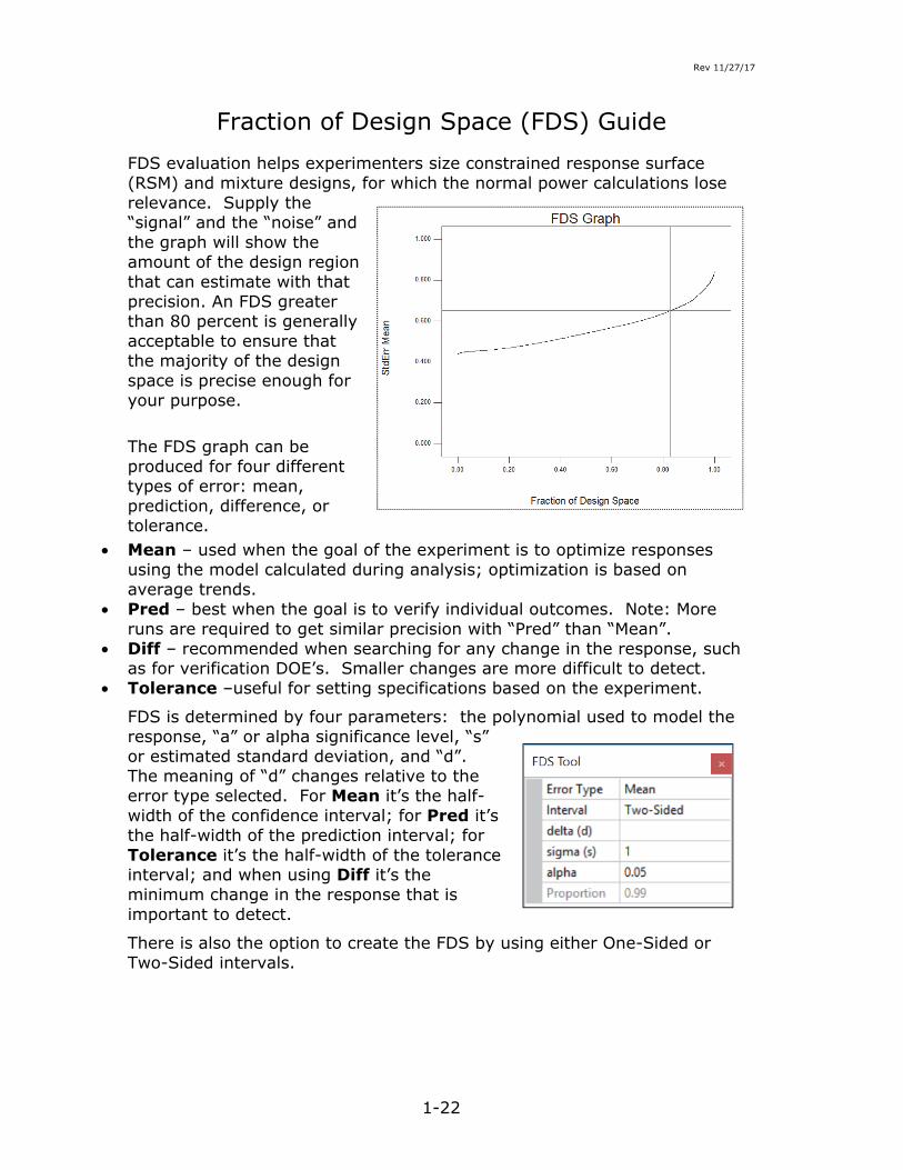
Factorial Analysis Guide 1. Compute effects. Use half-normal probability plot to select model. Click

the biggest effect (point furthest to the right) and continue right-to-left until the line runs through points nearest zero. Alternatively, on the Pareto Chart pick effects from left to right, largest to smallest, until all other effects fall below the Bonferroni and/or t-value limit.

2. Choose ANOVA* (Analysis of Variance) and check the selected model:

*(For split plots via REML—Restricted Maximum Likelihood—with p-values fine-tuned via Kenward-Roger method.)

a) Review the ANOVA results.

P-value < 0.05: significant.

P-value > 0.10: not significant.

b) Examine the F tests on the regression coefficients. Look for terms that can be eliminated, i.e., terms having (Prob > F) > 0.10. Be sure to maintain hierarchy.

c) Examine the F tests for the lack of fit (available only with measures of pure error from replicated runs). If insignificant continue with the analysis. If lack of fit tests significant, look at the graphs to determine if a more complex model is necessary. If the model is useful as is, use it.

d) Check for “Adeq Precision” > 4. This is a signal to noise ratio (see formula in Response Surface Analysis Guide). (Not available for split plots.)

3. Refer to the Residual Analysis and Diagnostic Plots Guide. Verify the ANOVA assumptions by looking at the residual plots.

Half-Normal Plot

Hal

f-Nor

mal

% P

roba

bilit

y

|Effect|

0.00 5.41 10.81 16.22 21.63

015

102030

50

70

80

90

95

99

A

CD

AC

AD

Pareto Chart

t-Val

ue o

f |Ef

fect

|

Rank

0.00

2.45

4.90

7.34

9.79

Bonferroni Limit 3.82734

t-Value Limit 2.22814

1 2 3 4 5 6 7 8 9 10 11 12 13 14 15

A

AC

AD

D

C

Rev 11/27/17

2-2

4. Explore the region of interest: a) One Factor plot (don’t use b) Interaction plot (with

for factors involved in 95% Least Significant interactions): Difference (LSD) bars):

c) Cube plot (especially useful if three factors are significant):

d) Contour plot and 3D surface plot:

A: Temperature (deg C)

24.00 26.20 28.40 30.60 32.80 35.00

Filtr

atio

n R

ate

(gal

lons

/hr)

40

50

60

70

80

90

100

110 Warning! Factor involved in multiple interactions.

One Factor

A: Temperature (deg C)

C: Concentration (percent)

24.00 26.20 28.40 30.60 32.80 35.00

Filtr

atio

n R

ate

(gal

lons

/hr)

40

50

60

70

80

90

100

110

C-

C+

Interaction

CubeFiltration Rate (gallons/hr)

A: Temperature (deg C)

C: C

once

ntra

tion

(per

cent

)

D: Stir Rate (rpm)

A-: 24.00 A+: 35.00C-: 2.00

C+: 4.00

D-: 15.00

D+: 30.00

46.25

44.25

74.25

72.25

69.375

100.625

61.125

92.375

Rev 11/27/17

2-3

Response Surface/Mixture Analysis Guide 1. Select a model (skip this step for split plots):

a) “WARNING”: Note which models are aliased, these can not be selected.

b) “Fit Summary”: Focus on the “Suggested” model. c) “Sequential Model Sum of Squares”: Select the highest order

polynomial where the additional terms are significant and the model is not aliased.

p-value < 0.05 p-value > 0.10 d) “Model Summary Statistics”: Focus on the model with high

“Adjusted R-Squared” and high “Predicted R-Squared”.

e) “Lack of Fit Tests”: Want the selected model to have insignificant lack-of-fit.

p-value < 0.05 p-value > 0.10

No lack-of-fit reported? If so, the design lacks: i. Excess unique points beyond the number of model terms (to

estimate variation about fitted surface), and/or ii. Replicate runs to estimate pure error (needed to statistically

assess the lack of fit).

2. Check the selected model: a) Review the ANOVA (for split plots use REML—Restricted Maximum

Likelihood—with p-values fine-tuned via Kenward-Roger method). The F-test is for the complete model, rather than just the additional terms for that order model as in the sequential table. Model should be significant (p-value < 0.05) and lack-of-fit insignificant (P-value > 0.10).

b) Examine the F tests on the regression coefficients - can the complexity of the polynomial be reduced? Look for terms that can be eliminated, i.e., coefficients having p-values > 0.10. Be sure to maintain hierarchy. If there are many such terms, consider using Auto Select.

c) Check for “Adeq Precision” > 4 (not available for split plots). This is a signal to noise ratio given by the following formula:

( ) ( )( ) ( ) ( )

=

==>

− n

i npYV

nYV

YV

YY1

2ˆ1ˆ4

ˆˆminˆmax σ

p = number of model parameters (including intercept (b0) and any block coefficients)

σ2 = residual MS from ANOVA table

n = number of experiments

Rev 11/27/17

2-4

d) Check that "Pred R-Squared" (not available for split plots) falls no more than 0.2 below the "Adj R-Squared". If so, consider model reduction.

3. Refer to the Residual Analysis and Diagnostics Plots Guide. Verify the ANOVA assumptions by looking at the residual plots.

4. Explore the region of interest: a) Perturbation/Trace plots to choose the factor(s)/component(s) to

“slice” through the design space. Choose ones having small effects (flat response curve) or components having linear effects (straight). In the RSM and mixture examples below, take slices of factor “A”.

RSM perturbation plot

Mixture trace plot (view Piepel’s direction for broadest paths)

Perturbation/Trace plots are particularly useful after finding optimal points. They show how sensitive the optimum is to changes in each factor or component.

-1.000 -0.500 0.000 0.500 1.000

50.0

60.0

70.0

80.0

90.0

100.0

AAB

B

C

C

Perturbation

Deviation from Reference Point (Coded Units)

Con

vers

ion

(%)

90

50

70

30

10

90

50

70

30

10

90

50

70

30

10

X1

X2 X3

90

50

70

30

10

90

50

70

30

10

90

50

70

30

10

90

50

70

30

10

90

50

70

30

10

90

50

70

30

10

X1

X2 X3

-0.400 -0.200 0.000 0.200 0.400 0.600 0.800

20

40

60

80

100

120

140

160

AA

B

B

C

C

Trace (Piepel)

Deviation from Reference Blend (L_Pseudo Units)

Visc

osity

(mPa

-sec

)

Rev 11/27/17

2-5

b) Contour plots (shown below for a mixture design) to explore your design space, slicing on the factors/components identified from the perturbation/trace plots as well as any categorical factors.

5. Perform “Numerical” optimization to identify most desirable factor

(component) levels for single or multiple responses. View the feasible window (‘sweet spot’) via “Graphical” optimization (‘overlay’ plot). See Optimization Guide for details.

6. See the Confirmation node under the Post Analysis branch for the prediction interval (PI) expected for individual confirmation runs. Perform a number—six is good—of confirmation runs, enter them in to generate their mean in comparison to the PI recalculated for the sample size. Ideally it will fall within range. If not, consider what may have changed between the time you did the experiment and the subsequent confirmation runs.

Rev 11/27/17

2-6

Combined Mixture/Process Analysis Guide 1. Select a model (skip this step for split plots): Look for what’s suggested

in the Fit Summary table, in this case: quadratic mixture by linear process (QxL). Often, as in this case, it’s the one with the highest adjusted and predicted R-squared (row [12] 0.9601 and 0.9240).

Combined Model Fit Summary Table

Mixture Order

Process Order

Mixture p-value

Process p-value

Adjusted R²

Predicted R²

1 M M

2 M L < 0.0001 0.3916 0.3329

3 M 2FI

0.9883 0.3561 0.2507

4 M Q * * 0.3561 0.2507 *Aliased

5 M C * 0.8488 0.3432 0.2198 *Aliased

6 L M < 0.0001 0.4460 0.3919

7 L L < 0.0001 < 0.0001 0.9211 0.8889

8 L 2FI < 0.0001 0.6237 0.9177 0.8341

9 L Q < 0.0001 0.9177 0.8341 Aliased

10 L C < 0.0001 0.9176 0.9113 0.7729 Aliased

11 Q M 0.5401 0.4373 0.3487

12 Q L 0.0003 < 0.0001 0.9601 0.9240 Suggested

13 Q 2FI 0.0028 0.1129 0.9736 0.8796

14 Q Q 0.0028 * 0.9736 0.8796 *Aliased

15 Q C 0.0389 0.7158 0.9683 -0.9445 Aliased

16 SC M 0.6426

0.4284 0.3348

17 SC L 0.4611 < 0.0001 0.9598 0.9181

18 SC 2FI 0.2567 0.1212 0.9802 0.8391

19 SC Q 0.2567 * 0.9802 0.8391 *Aliased

20 SC C * *

*Aliased

Rev 11/27/17

2-7

This sequential table shows the significance of terms added layer-by-layer to the model above. For example, in this case starting with the mean by mean (MxM) model (row [1]):

♦ Linear (L) process terms provide significant information beyond the mean (M) model (p<0.0001 in row [2]).

♦ Adding 2FI process terms provides no benefit ([3] p=0.9883). ♦ The next two models (rows [4] and [5]), MxQ and MxC are aliased

– do not pick them! ♦ Start again from MxM. ♦ Linear (L) mixture terms are significant ([6] p<0.0001). ♦ L process terms are a significant addition ([7] p<0.0001). ♦ 2FI process terms do not add significantly ([8] p=0.6237). ♦ The next two models ([9] and [10]), LxQ and LxC are aliased. ♦ Adding the Q-Mix terms provides no benefit ([11] p=0.5401). ♦ Add L process terms to significantly improve the model fit ([12]

p<0.0001). ♦ Adding the 2FI terms provide little benefit ([13] p=0.1129) and

they reduce the predicted R2. Thus, the QxL combined mixture-by-process model is suggested.

2. Due to the complexity of combined models, try Automatic Model Selection to remove unnecessary terms from the model.

See the next page for the details of automatic model selection.

Rev 11/27/17

2-8

Automatic Model Selection Automatic Model Selection is used to algorithmically choose the terms to keep in the model. There are four criterion that can be used: AICc, BIC, p-value, and Adjusted R-Squared. There are four selection methods: Forward, Backward, Stepwise and All Hierarchical. The table below shows the eight available combinations.

Selection

Forward Backward Stepwise All Hierarchical

Crite

rion AICc Yes* Yes* No No

BIC Yes* Yes* No No p-value Yes Yes* Yes No Adjusted R-Squared No No No Yes

* Best selection method for the given criterion

Automatic Model Selection cannot substitute for your judgment based on subject-matter knowledge. Please take the time to review the results on the ANOVA and Diagnostics before using the analysis to make decisions.

You are encouraged to use multiple combinations of the criterion and selection directions to help decide which terms form the best model. AICc with forward selection is the default and best general method for selecting the model. We suggest you also try a backward AICc selection. P-value using backward selection is also recommended and may be more familiar.

Details on Criterion: • AICc stands for Akaike Information Criterion corrected for a small

design. Akaike is pronounced (ah kah ee Kay). • BIC stands for Bayesian Information Criterion. It is an alternative to

AICc and is usually better for larger designs and models. • p-value is the standard method looking for significant terms to keep

and/or insignificant terms to remove from the model. • Adjusted R-squared is a statistic related to how well the current

model explains the data with an adjustment to prevent too many terms.

Details on Selection: • Forward selection seeks to add terms to a model that improve the

criterion. • Backward selection seeks to remove terms from a model that are

detrimental to the criterion. • Stepwise selection works by first including terms that improve the

criterion, then rechecks to see if any terms need to be removed. It is a combination of forward and backward.

• All Hierarchical selection checks all possible models that maintain hierarchy, keeping the one with the best criterion score.

Rev 11/27/17

2-9

Residual Analysis and Diagnostic Plots Guide Residual analysis is necessary to confirm that the assumptions for the ANOVA are met. Other diagnostic plots may provide interesting information in some situations. ALWAYS review these plots!

A. Diagnostic plots

1. Plot the (externally) studentized residuals:

a) Normal plot - should be straight line.

BAD: S shape GOOD: Linear or Normal

b) Residuals (ei) vs predicted - should be random scatter.

BAD: Megaphone shape GOOD: Random scatter

-2.14 -0.90 0.34 1.58 2.81

1

5

10

20

30

50

70

80

90

95

99

-1.60 -0.73 0.14 1.01 1.88

1

5

10

20

30

50

70

80

90

95

99

Rev 11/27/17

2-10

c) Residuals (ei) vs run - should be random scatter, no trends.

BAD: Trend GOOD: No pattern

Also, look for externally studentized residuals outside limits. These runs are statistical outliers that may indicate:

♦ a problem with the model,

♦ a transformation,

♦ a special cause that merits ignoring the result or run.

2. View the predicted vs actual plot whose points should be randomly scattered along the 45-degree line. Groups of points above or below the line indicate areas of over or under prediction.

Poor Prediction Better Prediction

Actual

Pred

icte

d

36.00

49.50

63.00

76.50

90.00

36.80 50.05 63.31 76.56 89.81

Actual

Pred

icte

d

36.00

48.75

61.50

74.25

87.00

36.80 49.22 61.65 74.08 86.50

Rev 11/27/17

2-11

3. Use the Box-Cox plot to determine if a power law transformation might be appropriate for your data. The blue line indicates the current transformation (at Lambda =1 for none) and the green line indicates the best lambda value. Red lines indicate a 95% confidence interval associated with the best lambda value. Stat-Ease software recommends the standard transformation, such as log, closest to the best lambda value unless the confidence interval includes 1, in which case the recommendation will be “None.”

Before Transformation After Transformation

4. Residuals (ei) vs factor – especially useful with blocks. Should be split by the zero-line at either end of the range – no obvious main effect (up or down). If you see an effect, go back, add it to the predictive model and assess its statistical significance. Relatively similar variation between levels. Watch ONLY for very large differences.

BAD: More variation at one end GOOD: Random scatter both ends

Rev 11/27/17

2-12

Influence plots

1. Cook’s Distance helps if you see more than one outlier in other diagnostic plots. Investigate the run with the largest Cook’s Distance first. Often, if this run is ignored due to a special cause, other apparent outliers can be explained by the model.

2. Watch for leverage vs run values at or beyond twice the average leverage. These runs will unduly influence at least one model parameter. If identified prior to running the experiment, it can be replicated to reduce leverage. Otherwise all you can do is check the actual responses to be sure they are as expected for the factor settings. Be especially careful of any leverages at one (1.0). These runs will be fitted exactly with no residual!

BAD: Some at twice the average GOOD: All the same

3. Deletion diagnostics – statistics calculated by taking each run out, one after the other, and seeing how this affects the model fit.

a) DFFITS (difference in fits) is another statistic helpful for detecting influential runs. Do not be overly alarmed at points outside of limits: Just check that they are not extraordinary. If earlier

Run Number

Leve

rage

0.00

0.25

0.50

0.75

1.00

1 6 11 16 21 26

Run Number

Leve

rage

g

0.0000

0.2500

0.5000

0.7500

1.0000

1 3 5 7 9 11 13 15 17

Run Number

Coo

k's

Dis

tanc

e

0.00

0.25

0.50

0.75

1.00

1 4 7 10 13 16

Rev 11/27/17

2-13

diagnostics show outliers that do not go out of bounds on DFFITS, then these do not create a significant difference in fits and thus you need not be overly concerned.

b) DFBETAS (difference in beta coefficients) breaks down the impact of any given run on a particular model term. If you see an excessive value, consider whether a factor in the term falls beyond a reasonable range (for example, it may be that an axial (star) point in a CCD projects outside of the feasible operating region) and, if so, try ignoring this particular run.

Statistical Details on Diagnostic Measures

Residual ( i i iˆe=y -y ):

Difference between the actual individual value ( iy ) and the value predicted from the model ( iy ).

Leverage ( ( ) i1TT

iii xXXxh −= where x is factor level and X is design matrix):

Numerical value between 0 and 1 that indicates the potential for a case to influence the model fit. A leverage of 1 means the predicted value at that particular case will exactly equal the observed value of the experiment (residual=0.) The sum of leverage values across all cases (design points) equals the number of coefficients (including the constant) fit by the model. The maximum leverage an experiment can have is 1/k, where k is the number of times the experiment is replicated. Values larger than 2 times the average leverage are flagged.

Internally Studentized Residual (( )

ii

ii

ers 1 h

=−

):

The residual divided by the estimated standard deviation of that residual (dependent on leverage), which measures the number of standard deviations separating the actual from predicted values.

Externally Studentized Residual ( ii

1 ii

ets 1 h−

=−

):

This “outlier t” value is calculated by leaving the run in question out of the analysis and estimating the response from the remaining runs. It represents the number of standard deviations between this predicted value

Rev 11/27/17

2-14

and the actual response. Runs with large t values (rule-of-thumb: |t| > 3.5) are flagged and should be investigated.

Note: For verification runs, this is calculated using the predicted error (an expansion of the hat matrix).

DFFITS ( i i, ii

1 ii

ˆ ˆy yDFFITS

s h−

−

−= , alternatively

1/2

iii i

ii

hDFFITS t1 h

= − ):

DFFFITS measures the influence each individual case (i) has on the predicted value (see Myers2 page 284.) It is a function of leverage (h). Mathematically it is the studentized difference between the predicted value with and without observation “i”. As shown by the alternative formula, DFFITS represents the externally studentized residual (ti) magnified by high leverage points and shrunk by low leverage points. Note that DFFITs becomes undefined for leverages of one (h=1).

DFBETAS ( j j, ij,i

1 jj

yDFBETAS

s c−

−

β −= , cjj is the jth diagonal element of (X’X)-1):

DFBETAS measures the influence each individual case (i) has on each model coefficient (βj). It represents the number of standard errors that the jth beta-coefficient changes if the ith observation is removed. Like DFFITS, this statistic becomes undefined for leverages of one (h=1). DFBETAS are calculated for each beta-coefficient, so make sure to use the pull-down menu and click through the terms (the down arrow is a good shortcut key – also, try the wheel if you have one on your mouse).

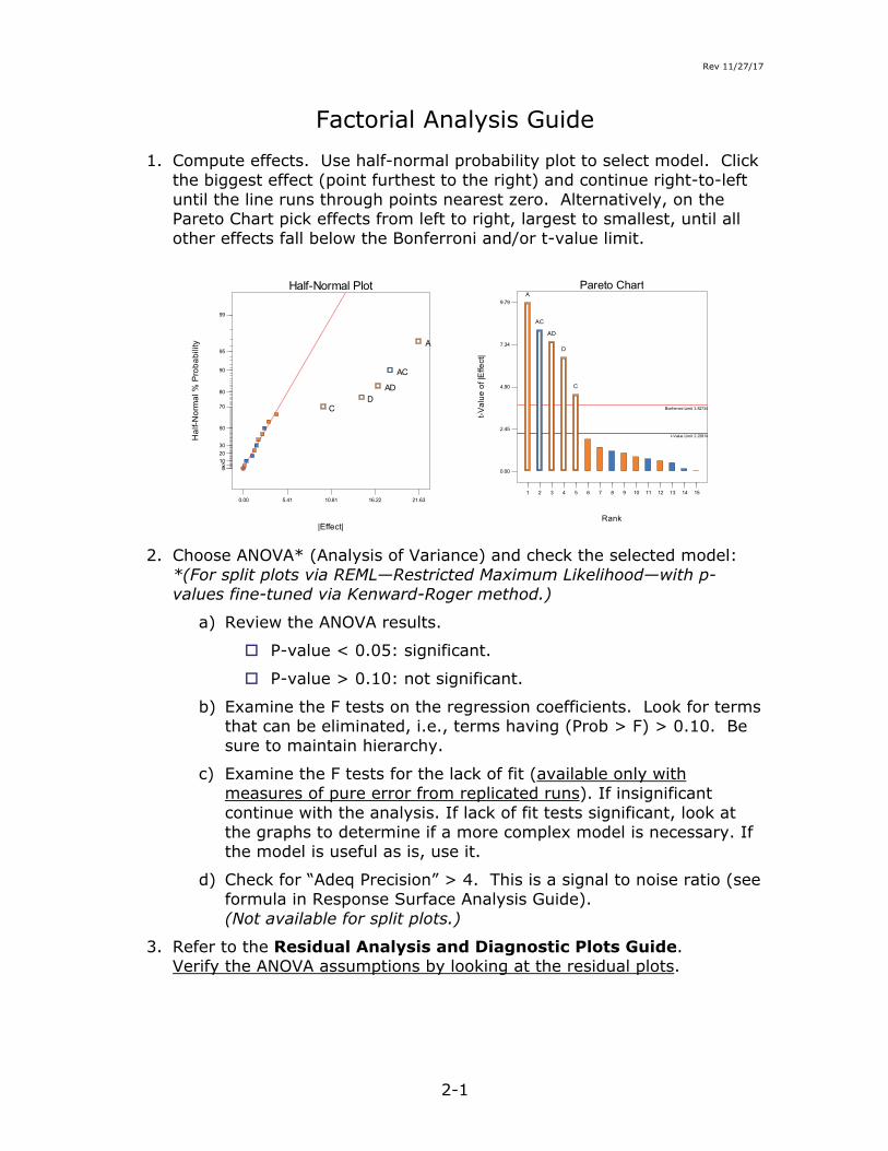
Cook's Distance ( 2 iii i

ii

h1D rp 1 h

= −

):

A measure of how much the regression would change if the case is omitted from the analysis (see Weisberg1 page 118). Relatively large values are associated with cases with high leverage and large studentized residuals. Cases with large Di values relative to the other cases should be investigated. Look for mistakes in recording, an incorrect model, or a design point far from the others.

References:

1. Weisberg, Stanford: Applied Linear Regression, 3rd edition, 2005, John Wiley & Sons, Inc.

2. Myers, Raymond: Classical and Modern Regression with Applications, 2nd edition, 2000, Duxbury Press.

Rev 11/27/17

2-15

Optimization Guide Numerical Optimization:

1. Analyze each response separately and establish an appropriate transformation and model for each. Be sure the fitted surface adequately represents your process. Check for:

a) A significant model, i.e., a large F-value with p<0.05.

b) Insignificant lack-of-fit, i.e., an F-value near one with p>0.10.

c) Adequate precision, i.e., greater than 4.

d) Well-behaved residuals.

2. Set the following criteria for the desirability optimization:

a) Goal: “maximize”, “minimize”, “target”, “in-range” and “Cpk”. Responses-only: “none” (default). Factors-only (default “in range”): “equal-to”.

b) Limits lower and upper: Both ends required to establish the desirability from 0 or 1.

c) Weight (optional): Enter 0.1 to 10 or drag the desirability ramp up (lighter) or down (heavier). The default of 1 keeps it linear. Weights >1 give more emphasis to the goal and vice-versa.

d) Importance (optional): Changes goal’s importance less (+) to more (+++++) relative to the others (default +++).

3. Run the optimization (press Solutions).

♦ Report shows settings of the factors, response values, and desirability for each solution from top to bottom.

♦ Ramps show settings for all factors and the resulting predicted values for responses and where these fall on their desirability ramps. Cycle through rank of solution from top to bottom.

♦ Bar Graph displays how well each variable satisfied their criterion.

4. Graph the desirability (shown) and the individual .

Rev 11/27/17

2-16

Graphical Optimization:

1. Criteria require at least one limit for at least one response:

2. Lower only if maximized (unlike numerical optimization where you must enter both lower and upper limits!)

♦ Upper only if minimized

♦ Lower and upper (specification range) if goal is target.

3. Graph the optimal point identified in the numerical optimization by clicking the #1 solution. It overlays all responses – shaded areas do not meet the specified criteria. The flagged window shows the “sweet spot”. For a more conservative result, put in the confidence interval (CI) shown here or, for quality by design (QbD), the tolerance interval (TI).

Suggestions for achieving desirable outcome:

Numerical optimization provides powerful insights when combined with graphical analysis. However, it cannot substitute for subject matter knowledge. For example, you may define what you consider to be optimum, only to find zero desirability everywhere! To avoid finding no optimums, set broad optimization criteria and then narrow down as you gain knowledge. Most often, multiple passes are needed to find the “best” factor levels to simultaneously satisfy all operational constraints.

40 42 44 46 48 50

2

2.2

2.4

2.6

2.8

3Overlay Plot

A: time (min.)

C: c

atal

yst (

%)

Conversion: 80

Conversion: 80

Conversion CI: 80

Conversion CI: 80

Activity: 60

Activity: 66

Activity CI: 60

Activity CI: 66

Conversion: 91.3165 CI Low: 87.6778 Activity: 62.9995 CI Low: 62.3401 CI High: 63.6589 X1 47.0146 X2 2.68444

Rev 11/27/17

Inverses, 1st & 2nd Derivatives of Transformations

Transform Square root counts

Loge

variation Log10

variation Inverse

square root Power

(lambda) 0.5 0 0 -0.5

Formula y = y+k′ ( )y ln y k′ = + ( )y log y k′ = + 1y =

y+k′

Inverse 2y y k′= − yy e k′= − yy 10 k′= − 2y y k−′= −

1st Derivative

y 2yy

∂ ′=′∂

( ) y yy ln e e ey

′ ′∂ = =′∂

( ) yy ln 10 10y

′∂ =′∂

3y 2yy

−∂ ′= −′∂

2nd Derivative

∂ =∂

2

2y 2

y '

∂ =∂

2y '

2y e

y ' ( )( )∂ =

∂

2 2 y '2y ln 10 10

y ' −∂ =

∂

24

2y 6y '

y '

Transform Inverse Rates

Power when all else fails

ArcSin Square Root Binomial data

y is a fraction (0-1) y’ in radians

Logit Asymptotically bounded data LL=lower limit UL=upper limit

Power (lambda) -1 λ NA NA

Formula 1y =

y+k′ ( )y = y+k λ′ -1y =sin y′

y LLy =lnUL y −′ −

Inverse 1y y k−′= − ( )1

y y kλ′= + ( ) 2y=(sin y )′ ( )y

y

UL e LLy

1 e

′

′

+=

+

1st Derivative

2y yy

−∂ ′= −′∂

( )1 1y 1 y

y

− λ ∂ ′=

′∂ λ ( ) ( )y 2sin y cos y

y∂ ′ ′=

′∂

( )( )y

2y

e UL LLyy 1 e

′

′

−∂ =′∂ +

2nd Derivative

−∂ =∂

23

2y 2y '

y ' ( )

− λ ∂ = − ∂ λ λ

2 1 22y 1 1 1 y '

y' ( )∂ =

∂

2

2y 2cos 2y '

y'

( )( )( )

− −∂ =∂ +

y ' y '2

32 y '

e 1 e UL LLyy' 1 e

Rev 11/27/17

Section 3:

Appendix

Rev 11/27/17

This page left blank intentionally as a spacer.

Rev 11/27/17

3-1

Z-Table:

Tail area of unit normal distribution z 0.00 0.01 0.02 0.03 0.04 0.05 0.06 0.07 0.08 0.09

0.0 0.5000 0.4960 0.4920 0.4880 0.4840 0.4801 0.4761 0.4721 0.4681 0.4641 0.1 0.4602 0.4562 0.4522 0.4483 0.4443 0.4404 0.4364 0.4325 0.4286 0.4247 0.2 0.4207 0.4168 0.4129 0.4090 0.4052 0.4013 0.3974 0.3936 0.3897 0.3859 0.3 0.3821 0.3783 0.3745 0.3707 0.3669 0.3632 0.3594 0.3557 0.3520 0.3483 0.4 0.3446 0.3409 0.3372 0.3336 0.3300 0.3264 0.3228 0.3192 0.3156 0.3121 0.5 0.3085 0.3050 0.3015 0.2981 0.2946 0.2912 0.2877 0.2843 0.2810 0.2776 0.6 0.2743 0.2709 0.2676 0.2643 0.2611 0.2578 0.2546 0.2514 0.2483 0.2451 0.7 0.2420 0.2389 0.2358 0.2327 0.2296 0.2266 0.2236 0.2206 0.2177 0.2148 0.8 0.2119 0.2090 0.2061 0.2033 0.2005 0.1977 0.1949 0.1922 0.1894 0.1867 0.9 0.1841 0.1814 0.1788 0.1762 0.1736 0.1711 0.1685 0.1660 0.1635 0.1611 1.0 0.1587 0.1562 0.1539 0.1515 0.1492 0.1469 0.1446 0.1423 0.1401 0.1379 1.1 0.1357 0.1335 0.1314 0.1292 0.1271 0.1251 0.1230 0.1210 0.1190 0.1170 1.2 0.1151 0.1131 0.1112 0.1093 0.1075 0.1056 0.1038 0.1020 0.1003 0.0985 1.3 0.0968 0.0951 0.0934 0.0918 0.0901 0.0885 0.0869 0.0853 0.0838 0.0823 1.4 0.0808 0.0793 0.0778 0.0764 0.0749 0.0735 0.0721 0.0708 0.0694 0.0681 1.5 0.0668 0.0655 0.0643 0.0630 0.0618 0.0606 0.0594 0.0582 0.0571 0.0559 1.6 0.0548 0.0537 0.0526 0.0516 0.0505 0.0495 0.0485 0.0475 0.0465 0.0455 1.7 0.0446 0.0436 0.0427 0.0418 0.0409 0.0401 0.0392 0.0384 0.0375 0.0367 1.8 0.0359 0.0351 0.0344 0.0336 0.0329 0.0322 0.0314 0.0307 0.0301 0.0294 1.9 0.0287 0.0281 0.0274 0.0268 0.0262 0.0256 0.0250 0.0244 0.0239 0.0233 2.0 0.0228 0.0222 0.0217 0.0212 0.0207 0.0202 0.0197 0.0192 0.0188 0.0183 2.1 0.0179 0.0174 0.0170 0.0166 0.0162 0.0158 0.0154 0.0150 0.0146 0.0143 2.2 0.0139 0.0136 0.0132 0.0129 0.0125 0.0122 0.0119 0.0116 0.0113 0.0110 2.3 0.0107 0.0104 0.0102 0.0099 0.0096 0.0094 0.0091 0.0089 0.0087 0.0084 2.4 0.0082 0.0080 0.0078 0.0075 0.0073 0.0071 0.0069 0.0068 0.0066 0.0064 2.5 0.0062 0.0060 0.0059 0.0057 0.0055 0.0054 0.0052 0.0051 0.0049 0.0048 2.6 0.0047 0.0045 0.0044 0.0043 0.0041 0.0040 0.0039 0.0038 0.0037 0.0036 2.7 0.0035 0.0034 0.0033 0.0032 0.0031 0.0030 0.0029 0.0028 0.0027 0.0026 2.8 0.0026 0.0025 0.0024 0.0023 0.0023 0.0022 0.0021 0.0021 0.0020 0.0019 2.9 0.0019 0.0018 0.0018 0.0017 0.0016 0.0016 0.0015 0.0015 0.0014 0.0014

3.0 0.0013 0.0013 0.0013 0.0012 0.0012 0.0011 0.0011 0.0011 0.0010 0.0010 3.1 0.0010 0.0009 0.0009 0.0009 0.0008 0.0008 0.0008 0.0008 0.0007 0.0007 3.2 0.0007 0.0007 0.0006 0.0006 0.0006 0.0006 0.0006 0.0005 0.0005 0.0005 3.3 0.0005 0.0005 0.0005 0.0004 0.0004 0.0004 0.0004 0.0004 0.0004 0.0003 3.4 0.0003 0.0003 0.0003 0.0003 0.0003 0.0003 0.0003 0.0003 0.0003 0.0002 3.5 0.0002 0.0002 0.0002 0.0002 0.0002 0.0002 0.0002 0.0002 0.0002 0.0002 3.6 0.0002 0.0002 0.0001 0.0001 0.0001 0.0001 0.0001 0.0001 0.0001 0.0001 3.7 0.0001 0.0001 0.0001 0.0001 0.0001 0.0001 0.0001 0.0001 0.0001 0.0001 3.8 0.0001 0.0001 0.0001 0.0001 0.0001 0.0001 0.0001 0.0001 0.0001 0.0001 3.9 0.0000 0.0000 0.0000 0.0000 0.0000 0.0000 0.0000 0.0000 0.0000 0.0000

Rev 11/27/17

3-2

One-tailed / Two-tailed t-Table Probability points of the t-distribution with df degrees of freedom

tail area probability 1-tail 0.40 0.25 0.10 0.05 0.025 0.01 0.005 0.0025 0.001 0.0005 2-tail 0.80 0.50 0.20 0.10 0.050 0.02 0.010 0.0050 0.002 0.0010

df=1 0.325 1.000 3.078 6.314 12.706 31.821 63.657 127.32 318.31 636.62 2 0.289 0.816 1.886 2.920 4.303 6.965 9.925 14.089 22.326 31.598 3 0.277 0.765 1.638 2.353 3.182 4.541 5.841 7.453 10.213 12.924 4 0.271 0.741 1.533 2.132 2.776 3.747 4.604 5.598 7.173 8.610 5 0.267 0.727 1.476 2.015 2.571 3.365 4.032 4.773 5.893 6.869 6 0.265 0.718 1.440 1.943 2.447 3.143 3.707 4.317 5.208 5.959 7 0.263 0.711 1.415 1.895 2.365 2.998 3.499 4.029 4.785 5.408 8 0.262 0.706 1.397 1.860 2.306 2.896 3.355 3.833 4.501 5.041 9 0.261 0.703 1.383 1.833 2.262 2.821 3.250 3.690 4.297 4.781

10 0.260 0.700 1.372 1.812 2.228 2.764 3.169 3.581 4.144 4.587 11 0.260 0.697 1.363 1.796 2.201 2.718 3.106 3.497 4.025 4.437 12 0.259 0.695 1.356 1.782 2.179 2.681 3.055 3.428 3.930 4.318 13 0.259 0.694 1.350 1.771 2.160 2.650 3.012 3.372 3.852 4.221 14 0.258 0.692 1.345 1.761 2.145 2.624 2.977 3.326 3.787 4.140 15 0.258 0.691 1.341 1.753 2.131 2.602 2.947 3.286 3.733 4.073 16 0.258 0.690 1.337 1.746 2.120 2.583 2.921 3.252 3.686 4.015 17 0.257 0.689 1.333 1.740 2.110 2.567 2.898 3.222 3.646 3.965 18 0.257 0.688 1.330 1.734 2.101 2.552 2.878 3.197 3.610 3.922 19 0.257 0.688 1.328 1.729 2.093 2.539 2.861 3.174 3.579 3.883 20 0.257 0.687 1.325 1.725 2.086 2.528 2.845 3.153 3.552 3.850 21 0.257 0.686 1.323 1.721 2.080 2.518 2.831 3.135 3.527 3.819 22 0.256 0.686 1.321 1.717 2.074 2.508 2.819 3.119 3.505 3.792 23 0.256 0.685 1.319 1.714 2.069 2.500 2.807 3.104 3.485 3.767 24 0.256 0.685 1.318 1.711 2.064 2.492 2.797 3.091 3.467 3.745 25 0.256 0.684 1.316 1.708 2.060 2.485 2.787 3.078 3.450 3.725 26 0.256 0.684 1.315 1.706 2.056 2.479 2.779 3.067 3.435 3.707 27 0.256 0.684 1.314 1.703 2.052 2.473 2.771 3.057 3.421 3.690 28 0.256 0.683 1.313 1.701 2.048 2.467 2.763 3.047 3.408 3.674 29 0.256 0.683 1.311 1.699 2.045 2.462 2.756 3.038 3.396 3.659 30 0.256 0.683 1.310 1.697 2.042 2.457 2.750 3.030 3.385 3.646 40 0.255 0.681 1.303 1.684 2.021 2.423 2.704 2.971 3.307 3.551 60 0.254 0.679 1.296 1.671 2.000 2.390 2.660 2.915 3.232 3.460

120 0.254 0.677 1.289 1.658 1.980 2.358 2.617 2.860 3.160 3.373 ∞ 0.253 0.674 1.282 1.645 1.960 2.326 2.576 2.807 3.090 3.291

t

Rev 11/27/17

3-3

αχ 2χ 2

αArea =

Cumulative Distribution of Chi-Square

Probability of a Greater value df 0.995 0.99 0.975 0.95 0.90 0.75 0.50 0.25 0.10 0.05 0.025 0.01 0.005

1 0.001 0.004 0.016 0.102 0.455 1.32 2.71 3.84 5.02 6.64 7.88 2 0.010 0.020 0.051 0.103 0.211 0.575 1.39 2.77 4.61 5.99 7.38 9.21 10.60 3 0.072 0.115 0.216 0.352 0.584 1.21 2.37 4.11 6.25 7.82 9.35 11.35 12.84 4 0.207 0.297 0.484 0.711 1.06 1.92 3.36 5.39 7.78 9.49 11.14 13.28 14.86

5 0.412 0.554 0.831 1.15 1.61 2.68 4.35 6.63 9.24 11.07 12.83 15.09 16.75 6 0.676 0.872 1.24 1.64 2.20 3.46 5.35 7.84 10.65 12.59 14.45 16.81 18.55 7 0.989 1.24 1.69 2.17 2.83 4.26 6.35 9.04 12.02 14.07 16.01 18.48 20.28 8 1.34 1.65 2.18 2.73 3.49 5.07 7.34 10.22 13.36 15.51 17.54 20.09 21.96 9 1.74 2.09 2.70 3.33 4.17 5.90 8.34 11.39 14.68 16.92 19.02 21.67 23.59

10 2.16 2.56 3.25 3.94 4.87 6.74 9.34 12.55 15.99 18.31 20.48 23.21 25.19 11 2.60 3.05 3.82 4.58 5.58 7.58 10.34 13.70 17.28 19.68 21.92 24.73 26.76 12 3.07 3.57 4.40 5.23 6.30 8.44 11.34 14.85 18.55 21.03 23.34 26.22 28.30 13 3.57 4.11 5.01 5.89 7.04 9.30 12.34 15.98 19.81 22.36 24.74 27.69 29.82 14 4.08 4.66 5.63 6.57 7.79 10.17 13.34 17.12 21.06 23.69 26.12 29.14 31.32

15 4.60 5.23 6.26 7.26 8.55 11.04 14.34 18.25 22.31 25.00 27.49 30.58 32.80 16 5.14 5.81 6.91 7.96 9.31 11.91 15.34 19.37 23.54 26.30 28.85 32.00 34.27 17 5.70 6.41 7.56 8.67 10.09 12.79 16.34 20.49 24.77 27.59 30.19 33.41 35.72 18 6.27 7.02 8.23 9.39 10.87 13.68 17.34 21.61 25.99 28.87 31.53 34.81 37.16 19 6.84 7.63 8.91 10.12 11.65 14.56 18.34 22.72 27.20 30.14 32.85 36.19 38.58 20 7.43 8.26 9.59 10.85 12.44 15.45 19.34 23.83 28.41 31.41 34.17 37.57 40.00 21 8.03 8.90 10.28 11.59 13.24 16.34 20.34 24.94 29.62 32.67 35.48 38.93 41.40 22 8.64 9.54 10.98 12.34 14.04 17.24 21.34 26.04 30.81 33.92 36.78 40.29 42.80 23 9.26 10.20 11.69 13.09 14.85 18.14 22.34 27.14 32.01 35.17 38.08 41.64 44.18 24 9.89 10.86 12.40 13.85 15.66 19.04 23.34 28.24 33.20 36.42 39.36 42.98 45.56 25 10.52 11.52 13.12 14.61 16.47 19.94 24.34 29.34 34.38 37.65 40.65 44.31 46.93 26 11.16 12.20 13.84 15.38 17.29 20.84 25.34 30.44 35.56 38.89 41.92 45.64 48.29 27 11.81 12.88 14.57 16.15 18.11 21.75 26.34 31.53 36.74 40.11 43.20 46.96 49.65 28 12.46 13.57 15.31 16.93 18.94 22.66 27.34 32.62 37.92 41.34 44.46 48.28 50.99 29 13.12 14.26 16.05 17.71 19.77 23.57 28.34 33.71 39.09 42.56 45.72 49.59 52.34 30 13.79 14.95 16.79 18.49 20.60 24.48 29.34 34.80 40.26 43.77 46.98 50.89 53.67 40 20.71 22.16 24.43 26.51 29.05 33.66 39.34 45.62 51.81 55.76 59.34 63.69 66.77 50 27.99 29.71 32.36 34.76 37.69 42.94 49.34 56.33 63.17 67.51 71.42 76.15 79.49 60 35.53 37.49 40.48 43.19 46.46 52.29 59.34 66.98 74.40 79.08 83.30 88.38 91.95 70 43.28 45.44 48.76 51.74 55.33 61.70 69.33 77.58 85.53 90.53 95.02 100.43 104.22 80 51.17 53.54 57.15 60.39 64.28 71.15 79.33 88.13 96.58 101.88 106.63 112.33 116.32 90 59.20 61.75 65.65 69.13 73.29 80.63 89.33 98.65 107.57 113.15 118.14 124.12 128.30

100 67.33 70.07 74.22 77.93 82.36 90.13 99.33 109.14 118.50 124.34 129.56 135.81 140.17

Rev 11/27/17

3-4

F-Table for 10%

Percentage points of the F-distribution: upper 10% points

dfnum

dfden 1 2 3 4 5 6 7 8 9 10 15 20

1 39.863 49.500 53.593 55.833 57.240 58.204 58.906 59.439 59.858 60.195 61.220 61.740 2 8.526 9.000 9.162 9.243 9.293 9.326 9.349 9.367 9.381 9.392 9.425 9.441 3 5.538 5.462 5.391 5.343 5.309 5.285 5.266 5.252 5.240 5.230 5.200 5.184 4 4.545 4.325 4.191 4.107 4.051 4.010 3.979 3.955 3.936 3.920 3.870 3.844 5 4.060 3.780 3.619 3.520 3.453 3.405 3.368 3.339 3.316 3.297 3.238 3.207 6 3.776 3.463 3.289 3.181 3.108 3.055 3.014 2.983 2.958 2.937 2.871 2.836 7 3.589 3.257 3.074 2.961 2.883 2.827 2.785 2.752 2.725 2.703 2.632 2.595 8 3.458 3.113 2.924 2.806 2.726 2.668 2.624 2.589 2.561 2.538 2.464 2.425 9 3.360 3.006 2.813 2.693 2.611 2.551 2.505 2.469 2.440 2.416 2.340 2.298

10 3.285 2.924 2.728 2.605 2.522 2.461 2.414 2.377 2.347 2.323 2.244 2.201 11 3.225 2.860 2.660 2.536 2.451 2.389 2.342 2.304 2.274 2.248 2.167 2.123 12 3.177 2.807 2.606 2.480 2.394 2.331 2.283 2.245 2.214 2.188 2.105 2.060 13 3.136 2.763 2.560 2.434 2.347 2.283 2.234 2.195 2.164 2.138 2.053 2.007 14 3.102 2.726 2.522 2.395 2.307 2.243 2.193 2.154 2.122 2.095 2.010 1.962 15 3.073 2.695 2.490 2.361 2.273 2.208 2.158 2.119 2.086 2.059 1.972 1.924 16 3.048 2.668 2.462 2.333 2.244 2.178 2.128 2.088 2.055 2.028 1.940 1.891 17 3.026 2.645 2.437 2.308 2.218 2.152 2.102 2.061 2.028 2.001 1.912 1.862 18 3.007 2.624 2.416 2.286 2.196 2.130 2.079 2.038 2.005 1.977 1.887 1.837 19 2.990 2.606 2.397 2.266 2.176 2.109 2.058 2.017 1.984 1.956 1.865 1.814 20 2.975 2.589 2.380 2.249 2.158 2.091 2.040 1.999 1.965 1.937 1.845 1.794 21 2.961 2.575 2.365 2.233 2.142 2.075 2.023 1.982 1.948 1.920 1.827 1.776 22 2.949 2.561 2.351 2.219 2.128 2.060 2.008 1.967 1.933 1.904 1.811 1.759 23 2.937 2.549 2.339 2.207 2.115 2.047 1.995 1.953 1.919 1.890 1.796 1.744 24 2.927 2.538 2.327 2.195 2.103 2.035 1.983 1.941 1.906 1.877 1.783 1.730 25 2.918 2.528 2.317 2.184 2.092 2.024 1.971 1.929 1.895 1.866 1.771 1.718 26 2.909 2.519 2.307 2.174 2.082 2.014 1.961 1.919 1.884 1.855 1.760 1.706 27 2.901 2.511 2.299 2.165 2.073 2.005 1.952 1.909 1.874 1.845 1.749 1.695 28 2.894 2.503 2.291 2.157 2.064 1.996 1.943 1.900 1.865 1.836 1.740 1.685 29 2.887 2.495 2.283 2.149 2.057 1.988 1.935 1.892 1.857 1.827 1.731 1.676 30 2.881 2.489 2.276 2.142 2.049 1.980 1.927 1.884 1.849 1.819 1.722 1.667 40 2.835 2.440 2.226 2.091 1.997 1.927 1.873 1.829 1.793 1.763 1.662 1.605 60 2.791 2.393 2.177 2.041 1.946 1.875 1.819 1.775 1.738 1.707 1.603 1.543

120 2.748 2.347 2.130 1.992 1.896 1.824 1.767 1.722 1.684 1.652 1.545 1.482 100K 2.706 2.303 2.084 1.945 1.847 1.774 1.717 1.670 1.632 1.599 1.487 1.421

K (Multiply this value by 1000)

F10%

Rev 11/27/17

3-5

F-Table for 5% Percentage points of the F-distribution: upper 5% points

dfnum

dfden 1 2 3 4 5 6 7 8 9 10 15 20

1 161.45 199.50 215.71 224.58 230.16 233.99 236.77 238.88 240.54 241.88 245.95 248.01 2 18.513 19.000 19.164 19.247 19.296 19.330 19.353 19.371 19.385 19.396 19.429 19.446 3 10.128 9.552 9.277 9.117 9.013 8.941 8.887 8.845 8.812 8.786 8.703 8.660 4 7.709 6.944 6.591 6.388 6.256 6.163 6.094 6.041 5.999 5.964 5.858 5.803 5 6.608 5.786 5.409 5.192 5.050 4.950 4.876 4.818 4.772 4.735 4.619 4.558 6 5.987 5.143 4.757 4.534 4.387 4.284 4.207 4.147 4.099 4.060 3.938 3.874 7 5.591 4.737 4.347 4.120 3.972 3.866 3.787 3.726 3.677 3.637 3.511 3.445 8 5.318 4.459 4.066 3.838 3.687 3.581 3.500 3.438 3.388 3.347 3.218 3.150 9 5.117 4.256 3.863 3.633 3.482 3.374 3.293 3.230 3.179 3.137 3.006 2.936

10 4.965 4.103 3.708 3.478 3.326 3.217 3.135 3.072 3.020 2.978 2.845 2.774 11 4.844 3.982 3.587 3.357 3.204 3.095 3.012 2.948 2.896 2.854 2.719 2.646 12 4.747 3.885 3.490 3.259 3.106 2.996 2.913 2.849 2.796 2.753 2.617 2.544 13 4.667 3.806 3.411 3.179 3.025 2.915 2.832 2.767 2.714 2.671 2.533 2.459 14 4.600 3.739 3.344 3.112 2.958 2.848 2.764 2.699 2.646 2.602 2.463 2.388 15 4.543 3.682 3.287 3.056 2.901 2.790 2.707 2.641 2.588 2.544 2.403 2.328 16 4.494 3.634 3.239 3.007 2.852 2.741 2.657 2.591 2.538 2.494 2.352 2.276 17 4.451 3.592 3.197 2.965 2.810 2.699 2.614 2.548 2.494 2.450 2.308 2.230 18 4.414 3.555 3.160 2.928 2.773 2.661 2.577 2.510 2.456 2.412 2.269 2.191 19 4.381 3.522 3.127 2.895 2.740 2.628 2.544 2.477 2.423 2.378 2.234 2.155 20 4.351 3.493 3.098 2.866 2.711 2.599 2.514 2.447 2.393 2.348 2.203 2.124 21 4.325 3.467 3.072 2.840 2.685 2.573 2.488 2.420 2.366 2.321 2.176 2.096 22 4.301 3.443 3.049 2.817 2.661 2.549 2.464 2.397 2.342 2.297 2.151 2.071 23 4.279 3.422 3.028 2.796 2.640 2.528 2.442 2.375 2.320 2.275 2.128 2.048 24 4.260 3.403 3.009 2.776 2.621 2.508 2.423 2.355 2.300 2.255 2.108 2.027 25 4.242 3.385 2.991 2.759 2.603 2.490 2.405 2.337 2.282 2.236 2.089 2.007 26 4.225 3.369 2.975 2.743 2.587 2.474 2.388 2.321 2.265 2.220 2.072 1.990 27 4.210 3.354 2.960 2.728 2.572 2.459 2.373 2.305 2.250 2.204 2.056 1.974 28 4.196 3.340 2.947 2.714 2.558 2.445 2.359 2.291 2.236 2.190 2.041 1.959 29 4.183 3.328 2.934 2.701 2.545 2.432 2.346 2.278 2.223 2.177 2.027 1.945 30 4.171 3.316 2.922 2.690 2.534 2.421 2.334 2.266 2.211 2.165 2.015 1.932 40 4.085 3.232 2.839 2.606 2.449 2.336 2.249 2.180 2.124 2.077 1.924 1.839 60 4.001 3.150 2.758 2.525 2.368 2.254 2.167 2.097 2.040 1.993 1.836 1.748

120 3.920 3.072 2.680 2.447 2.290 2.175 2.087 2.016 1.959 1.910 1.750 1.659 100K 3.842 2.996 2.605 2.372 2.214 2.099 2.010 1.939 1.880 1.831 1.666 1.571

K (Multiply this value by 1000)

F5%

Rev 11/27/17

3-6

F-Table for 2.5% Percentage points of the F-distribution: upper 2.5% points

dfnum

dfden 1 2 3 4 5 6 7 8 9 10 15 20

1 647.79 799.50 864.16 899.58 921.85 937.11 948.22 956.66 963.28 968.63 984.87 993.10

2 38.506 39.000 39.165 39.248 39.298 39.331 39.355 39.373 39.387 39.398 39.431 39.448

3 17.443 16.044 15.439 15.101 14.885 14.735 14.624 14.540 14.473 14.419 14.253 14.167

4 12.218 10.649 9.979 9.605 9.364 9.197 9.074 8.980 8.905 8.844 8.657 8.560 5 10.007 8.434 7.764 7.388 7.146 6.978 6.853 6.757 6.681 6.619 6.428 6.329 6 8.813 7.260 6.599 6.227 5.988 5.820 5.695 5.600 5.523 5.461 5.269 5.168 7 8.073 6.542 5.890 5.523 5.285 5.119 4.995 4.899 4.823 4.761 4.568 4.467 8 7.571 6.059 5.416 5.053 4.817 4.652 4.529 4.433 4.357 4.295 4.101 3.999 9 7.209 5.715 5.078 4.718 4.484 4.320 4.197 4.102 4.026 3.964 3.769 3.667

10 6.937 5.456 4.826 4.468 4.236 4.072 3.950 3.855 3.779 3.717 3.522 3.419 11 6.724 5.256 4.630 4.275 4.044 3.881 3.759 3.664 3.588 3.526 3.330 3.226 12 6.554 5.096 4.474 4.121 3.891 3.728 3.607 3.512 3.436 3.374 3.177 3.073 13 6.414 4.965 4.347 3.996 3.767 3.604 3.483 3.388 3.312 3.250 3.053 2.948 14 6.298 4.857 4.242 3.892 3.663 3.501 3.380 3.285 3.209 3.147 2.949 2.844 15 6.200 4.765 4.153 3.804 3.576 3.415 3.293 3.199 3.123 3.060 2.862 2.756 16 6.115 4.687 4.077 3.729 3.502 3.341 3.219 3.125 3.049 2.986 2.788 2.681 17 6.042 4.619 4.011 3.665 3.438 3.277 3.156 3.061 2.985 2.922 2.723 2.616 18 5.978 4.560 3.954 3.608 3.382 3.221 3.100 3.005 2.929 2.866 2.667 2.559 19 5.922 4.508 3.903 3.559 3.333 3.172 3.051 2.956 2.880 2.817 2.617 2.509 20 5.871 4.461 3.859 3.515 3.289 3.128 3.007 2.913 2.837 2.774 2.573 2.464 21 5.827 4.420 3.819 3.475 3.250 3.090 2.969 2.874 2.798 2.735 2.534 2.425 22 5.786 4.383 3.783 3.440 3.215 3.055 2.934 2.839 2.763 2.700 2.498 2.389 23 5.750 4.349 3.750 3.408 3.183 3.023 2.902 2.808 2.731 2.668 2.466 2.357 24 5.717 4.319 3.721 3.379 3.155 2.995 2.874 2.779 2.703 2.640 2.437 2.327 25 5.686 4.291 3.694 3.353 3.129 2.969 2.848 2.753 2.677 2.613 2.411 2.300 26 5.659 4.265 3.670 3.329 3.105 2.945 2.824 2.729 2.653 2.590 2.387 2.276 27 5.633 4.242 3.647 3.307 3.083 2.923 2.802 2.707 2.631 2.568 2.364 2.253 28 5.610 4.221 3.626 3.286 3.063 2.903 2.782 2.687 2.611 2.547 2.344 2.232 29 5.588 4.201 3.607 3.267 3.044 2.884 2.763 2.669 2.592 2.529 2.325 2.213 30 5.568 4.182 3.589 3.250 3.026 2.867 2.746 2.651 2.575 2.511 2.307 2.195 40 5.424 4.051 3.463 3.126 2.904 2.744 2.624 2.529 2.452 2.388 2.182 2.068 60 5.286 3.925 3.343 3.008 2.786 2.627 2.507 2.412 2.334 2.270 2.061 1.944

120 5.152 3.805 3.227 2.894 2.674 2.515 2.395 2.299 2.222 2.157 1.945 1.825 ∞ 5.024 3.689 3.116 2.786 2.567 2.408 2.288 2.192 2.114 2.048 1.833 1.709

F2.5%

Rev 11/27/17

3-7

F-Table for 1%

Percentage points of the F-distribution: upper 1% points

dfnum

dfden 1 2 3 4 5 6 7 8 9 10 15 20

1 4052.2 4999.5 5403.3 5624.6 5763.6 5859.0 5928.3 5981.1 6022.5 6055.8 6157.3 6208.7 2 98.503 99.000 99.166 99.249 99.299 99.333 99.356 99.374 99.388 99.399 99.433 99.449 3 34.116 30.817 29.457 28.710 28.237 27.911 27.672 27.489 27.345 27.229 26.872 26.690 4 21.198 18.000 16.694 15.977 15.522 15.207 14.976 14.799 14.659 14.546 14.198 14.020 5 16.258 13.274 12.060 11.392 10.967 10.672 10.456 10.289 10.158 10.051 9.722 9.553 6 13.745 10.925 9.780 9.148 8.746 8.466 8.260 8.102 7.976 7.874 7.559 7.396 7 12.246 9.547 8.451 7.847 7.460 7.191 6.993 6.840 6.719 6.620 6.314 6.155 8 11.259 8.649 7.591 7.006 6.632 6.371 6.178 6.029 5.911 5.814 5.515 5.359 9 10.561 8.022 6.992 6.422 6.057 5.802 5.613 5.467 5.351 5.257 4.962 4.808

10 10.044 7.559 6.552 5.994 5.636 5.386 5.200 5.057 4.942 4.849 4.558 4.405 11 9.646 7.206 6.217 5.668 5.316 5.069 4.886 4.744 4.632 4.539 4.251 4.099 12 9.330 6.927 5.953 5.412 5.064 4.821 4.640 4.499 4.388 4.296 4.010 3.858 13 9.074 6.701 5.739 5.205 4.862 4.620 4.441 4.302 4.191 4.100 3.815 3.665 14 8.862 6.515 5.564 5.035 4.695 4.456 4.278 4.140 4.030 3.939 3.656 3.505 15 8.683 6.359 5.417 4.893 4.556 4.318 4.142 4.004 3.895 3.805 3.522 3.372 16 8.531 6.226 5.292 4.773 4.437 4.202 4.026 3.890 3.780 3.691 3.409 3.259 17 8.400 6.112 5.185 4.669 4.336 4.102 3.927 3.791 3.682 3.593 3.312 3.162 18 8.285 6.013 5.092 4.579 4.248 4.015 3.841 3.705 3.597 3.508 3.227 3.077 19 8.185 5.926 5.010 4.500 4.171 3.939 3.765 3.631 3.523 3.434 3.153 3.003 20 8.096 5.849 4.938 4.431 4.103 3.871 3.699 3.564 3.457 3.368 3.088 2.938 21 8.017 5.780 4.874 4.369 4.042 3.812 3.640 3.506 3.398 3.310 3.030 2.880 22 7.945 5.719 4.817 4.313 3.988 3.758 3.587 3.453 3.346 3.258 2.978 2.827 23 7.881 5.664 4.765 4.264 3.939 3.710 3.539 3.406 3.299 3.211 2.931 2.781 24 7.823 5.614 4.718 4.218 3.895 3.667 3.496 3.363 3.256 3.168 2.889 2.738 25 7.770 5.568 4.675 4.177 3.855 3.627 3.457 3.324 3.217 3.129 2.850 2.699 26 7.721 5.526 4.637 4.140 3.818 3.591 3.421 3.288 3.182 3.094 2.815 2.664 27 7.677 5.488 4.601 4.106 3.785 3.558 3.388 3.256 3.149 3.062 2.783 2.632 28 7.636 5.453 4.568 4.074 3.754 3.528 3.358 3.226 3.120 3.032 2.753 2.602 29 7.598 5.420 4.538 4.045 3.725 3.499 3.330 3.198 3.092 3.005 2.726 2.574 30 7.562 5.390 4.510 4.018 3.699 3.473 3.304 3.173 3.067 2.979 2.700 2.549 40 7.314 5.179 4.313 3.828 3.514 3.291 3.124 2.993 2.888 2.801 2.522 2.369 60 7.077 4.977 4.126 3.649 3.339 3.119 2.953 2.823 2.718 2.632 2.352 2.198

120 6.851 4.787 3.949 3.480 3.174 2.956 2.792 2.663 2.559 2.472 2.192 2.035 100K 6.635 4.605 3.782 3.319 3.017 2.802 2.640 2.511 2.408 2.321 2.039 1.878

K (Multiply this value by 1000)

F1%

Rev 11/27/17

3-8

F-Table for 0.5% Percentage points of the F-distribution: upper 0.5% points

dfnum

dfden 1 2 3 4 5 6 7 8 9 10 15 20

1 16210.7 19999.5 21614.7 22499.6 23055.8 23437.1 23714.6 23925.6 24091.0 24224.5 24630.2 24836.0

2 198.50 199.00 199.17 199.25 199.30 199.33 199.36 199.37 199.39 199.40 199.43 199.45 3 55.552 49.799 47.467 46.195 45.392 44.838 44.434 44.126 43.882 43.686 43.085 42.778 4 31.333 26.284 24.259 23.155 22.456 21.975 21.622 21.352 21.139 20.967 20.438 20.167 5 22.785 18.314 16.530 15.556 14.940 14.513 14.200 13.961 13.772 13.618 13.146 12.903 6 18.635 14.544 12.917 12.028 11.464 11.073 10.786 10.566 10.391 10.250 9.814 9.589 7 16.236 12.404 10.882 10.050 9.522 9.155 8.885 8.678 8.514 8.380 7.968 7.754 8 14.688 11.042 9.596 8.805 8.302 7.952 7.694 7.496 7.339 7.211 6.814 6.608 9 13.614 10.107 8.717 7.956 7.471 7.134 6.885 6.693 6.541 6.417 6.032 5.832

10 12.826 9.427 8.081 7.343 6.872 6.545 6.302 6.116 5.968 5.847 5.471 5.274 11 12.226 8.912 7.600 6.881 6.422 6.102 5.865 5.682 5.537 5.418 5.049 4.855 12 11.754 8.510 7.226 6.521 6.071 5.757 5.525 5.345 5.202 5.085 4.721 4.530 13 11.374 8.186 6.926 6.233 5.791 5.482 5.253 5.076 4.935 4.820 4.460 4.270 14 11.060 7.922 6.680 5.998 5.562 5.257 5.031 4.857 4.717 4.603 4.247 4.059 15 10.798 7.701 6.476 5.803 5.372 5.071 4.847 4.674 4.536 4.424 4.070 3.883 16 10.575 7.514 6.303 5.638 5.212 4.913 4.692 4.521 4.384 4.272 3.920 3.734 17 10.384 7.354 6.156 5.497 5.075 4.779 4.559 4.389 4.254 4.142 3.793 3.607 18 10.218 7.215 6.028 5.375 4.956 4.663 4.445 4.276 4.141 4.030 3.683 3.498 19 10.073 7.093 5.916 5.268 4.853 4.561 4.345 4.177 4.043 3.933 3.587 3.402 20 9.944 6.986 5.818 5.174 4.762 4.472 4.257 4.090 3.956 3.847 3.502 3.318 21 9.830 6.891 5.730 5.091 4.681 4.393 4.179 4.013 3.880 3.771 3.427 3.243 22 9.727 6.806 5.652 5.017 4.609 4.322 4.109 3.944 3.812 3.703 3.360 3.176 23 9.635 6.730 5.582 4.950 4.544 4.259 4.047 3.882 3.750 3.642 3.300 3.116 24 9.551 6.661 5.519 4.890 4.486 4.202 3.991 3.826 3.695 3.587 3.246 3.062 25 9.475 6.598 5.462 4.835 4.433 4.150 3.939 3.776 3.645 3.537 3.196 3.013 26 9.406 6.541 5.409 4.785 4.384 4.103 3.893 3.730 3.599 3.492 3.151 2.968 27 9.342 6.489 5.361 4.740 4.340 4.059 3.850 3.687 3.557 3.450 3.110 2.928 28 9.284 6.440 5.317 4.698 4.300 4.020 3.811 3.649 3.519 3.412 3.073 2.890 29 9.230 6.396 5.276 4.659 4.262 3.983 3.775 3.613 3.483 3.377 3.038 2.855 30 9.180 6.355 5.239 4.623 4.228 3.949 3.742 3.580 3.450 3.344 3.006 2.823 40 8.828 6.066 4.976 4.374 3.986 3.713 3.509 3.350 3.222 3.117 2.781 2.598 60 8.495 5.795 4.729 4.140 3.760 3.492 3.291 3.134 3.008 2.904 2.570 2.387

120 8.179 5.539 4.497 3.921 3.548 3.285 3.087 2.933 2.808 2.705 2.373 2.188 ∞ 7.880 5.299 4.280 3.715 3.350 3.091 2.897 2.745 2.621 2.519 2.187 2.000

F0.5%

Rev 11/27/17

3-9

F-Table for 0.1% Percentage points of the F-distribution: upper 0.1% points

dfnum

dfden 1 2 3 4 5 6 7 8 9 10 15 20

1 405.2K 500.0K 540.4K 562.5K 576.4K 585.9K 592.9K 598.1K 602.3K9605.6K 615.8K 620.9K 2 998.50 999.00 999.17 999.25 999.30 999.33 999.36 999.37 999.39 999.40 999.43 999.45 3 167.03 148.50 141.11 137.10 134.58 132.85 131.58 130.62 129.86 129.25 127.37 126.42 4 74.137 61.246 56.177 53.436 51.712 50.525 49.658 48.996 48.475 48.053 46.761 46.100 5 47.181 37.122 33.202 31.085 29.752 28.834 28.163 27.649 27.244 26.917 25.911 25.395 6 35.507 27.000 23.703 21.924 20.803 20.030 19.463 19.030 18.688 18.411 17.559 17.120 7 29.245 21.689 18.772 17.198 16.206 15.521 15.019 14.634 14.330 14.083 13.324 12.932 8 25.415 18.494 15.829 14.392 13.485 12.858 12.398 12.046 11.767 11.540 10.841 10.480 9 22.857 16.387 13.902 12.560 11.714 11.128 10.698 10.368 10.107 9.894 9.238 8.898 10 21.040 14.905 12.553 11.283 10.481 9.926 9.517 9.204 8.956 8.754 8.129 7.804 11 19.687 13.812 11.561 10.346 9.578 9.047 8.655 8.355 8.116 7.922 7.321 7.008 12 18.643 12.974 10.804 9.633 8.892 8.379 8.001 7.710 7.480 7.292 6.709 6.405 13 17.815 12.313 10.209 9.073 8.354 7.856 7.489 7.206 6.982 6.799 6.231 5.934 14 17.143 11.779 9.729 8.622 7.922 7.436 7.077 6.802 6.583 6.404 5.848 5.557 15 16.587 11.339 9.335 8.253 7.567 7.092 6.741 6.471 6.256 6.081 5.535 5.248 16 16.120 10.971 9.006 7.944 7.272 6.805 6.460 6.195 5.984 5.812 5.274 4.992 17 15.722 10.658 8.727 7.683 7.022 6.562 6.223 5.962 5.754 5.584 5.054 4.775 18 15.379 10.390 8.487 7.459 6.808 6.355 6.021 5.763 5.558 5.390 4.866 4.590 19 15.081 10.157 8.280 7.265 6.622 6.175 5.845 5.590 5.388 5.222 4.704 4.430 20 14.819 9.953 8.098 7.096 6.461 6.019 5.692 5.440 5.239 5.075 4.562 4.290 21 14.587 9.772 7.938 6.947 6.318 5.881 5.557 5.308 5.109 4.946 4.437 4.167 22 14.380 9.612 7.796 6.814 6.191 5.758 5.438 5.190 4.993 4.832 4.326 4.058 23 14.195 9.469 7.669 6.696 6.078 5.649 5.331 5.085 4.890 4.730 4.227 3.961 24 14.028 9.339 7.554 6.589 5.977 5.550 5.235 4.991 4.797 4.638 4.139 3.873 25 13.877 9.223 7.451 6.493 5.885 5.462 5.148 4.906 4.713 4.555 4.059 3.794 26 13.739 9.116 7.357 6.406 5.802 5.381 5.070 4.829 4.637 4.480 3.986 3.723 27 13.613 9.019 7.272 6.326 5.726 5.308 4.998 4.759 4.568 4.412 3.920 3.658 28 13.498 8.931 7.193 6.253 5.656 5.241 4.933 4.695 4.505 4.349 3.859 3.598 29 13.391 8.849 7.121 6.186 5.593 5.179 4.873 4.636 4.447 4.292 3.804 3.543 30 13.293 8.773 7.054 6.125 5.534 5.122 4.817 4.581 4.393 4.239 3.753 3.493 40 12.609 8.251 6.595 5.698 5.128 4.731 4.436 4.207 4.024 3.874 3.400 3.145 60 11.973 7.768 6.171 5.307 4.757 4.372 4.086 3.865 3.687 3.541 3.078 2.827 120 11.380 7.321 5.781 4.947 4.416 4.044 3.767 3.552 3.379 3.237 2.783 2.534 100K 10.828 6.908 5.422 4.617 4.103 3.743 3.475 3.266 3.098 2.959 2.513 2.266

K (Multiply entries by 1000 in first row of F values, and last value for df)

Rev 11/27/17

3-10

Factors for Two-Sided Tolerance Limits for Normal Distributions

Factors K2 such that the probability is γ (gamma) that at least a proportion P of the distribution will be included between ± 2Y K s.

γ = 0.75 n P = 0.75 P = 0.90 P = 0.95 P = 0.99 P = 0.999 2 4.498 6.301 7.414 9.531 11.920 3 2.501 3.538 4.187 5.431 6.844 4 2.035 2.892 3.431 4.471 5.657 5 1.825 2.599 3.088 4.033 5.117 6 1.704 2.429 2.889 3.779 4.802 7 1.624 2.318 2.757 3.611 4.593 8 1.568 2.238 2.663 3.491 4.444 9 1.525 2.178 2.593 3.400 4.330

10 1.492 2.131 2.537 3.328 4.241 11 1.465 2.093 2.493 3.271 4.169 12 1.443 2.062 2.456 3.223 4.110 13 1.425 2.036 2.424 3.183 4.059 14 1.409 2.013 2.398 3.148 4.016 15 1.395 1.994 2.375 3.118 3.979 16 1.383 1.977 2.355 3.092 3.946 17 1.372 1.962 2.337 3.069 3.917 18 1.363 1.948 2.321 3.048 3.891 19 1.355 1.936 2.307 3.030 3.867 20 1.347 1.925 2.294 3.013 3.846 21 1.340 1.915 2.282 2.998 3.827 22 1.334 1.906 2.271 2.984 3.809 23 1.328 1.898 2.261 2.971 3.793 24 1.322 1.891 2.252 2.959 3.778 25 1.317 1.883 2.244 2.948 3.764 26 1.313 1.877 2.236 2.938 3.751 27 1.309 1.871 2.229 2.929 3.739 28 1.305 1.865 2.222 2.920 3.728 29 1.301 1.860 2.216 2.911 3.718 30 1.297 1.855 2.210 2.904 3.708 35 1.283 1.834 2.185 2.871 3.667 40 1.271 1.818 2.166 2.846 3.635 45 1.262 1.805 2.150 2.826 3.609 50 1.255 1.794 2.138 2.809 3.588 75 1.231 1.760 2.098 2.756 3.521

100 1.218 1.742 2.075 2.727 3.484 200 1.195 1.709 2.037 2.677 3.419 500 1.177 1.683 2.006 2.636 3.368

1000 1.169 1.671 1.992 2.617 3.344 ∞ 1.150 1.645 1.960 2.576 3.291

Rev 11/27/17

3-11

Factors for Two-Sided Tolerance Limits for Normal Distributions

Factors K2 such that the probability is γ (gamma) that at least a proportion P of the distribution will be included between ± 2Y K s.

γ = 0.90 n P = 0.75 P = 0.90 P = 0.95 P = 0.99 P = 0.999 2 11.407 15.978 18.800 24.167 30.227 3 4.132 5.847 6.919 8.974 11.309 4 2.932 4.166 4.943 6.440 8.149 5 2.454 3.494 4.152 5.423 6.879 6 2.196 3.131 3.723 4.870 6.188 7 2.034 2.902 3.452 4.521 5.750 8 1.921 2.743 3.264 4.278 5.446 9 1.839 2.626 3.125 4.098 5.220

10 1.775 2.535 3.018 3.959 5.046 11 1.724 2.463 2.933 3.849 4.906 12 1.683 2.404 2.863 3.758 4.792 13 1.648 2.355 2.805 3.682 4.697 14 1.619 2.314 2.756 3.618 4.615 15 1.594 2.278 2.713 3.562 4.545 16 1.572 2.246 2.676 3.514 4.484 17 1.552 2.219 2.643 3.471 4.430 18 1.535 2.194 2.614 3.433 4.382 19 1.520 2.172 2.588 3.399 4.339 20 1.506 2.152 2.564 3.368 4.300 21 1.493 2.135 2.543 3.340 4.264 22 1.482 2.118 2.524 3.315 4.232 23 1.471 2.103 2.506 3.292 4.203 24 1.462 2.089 2.489 3.270 4.176 25 1.453 2.077 2.474 3.251 4.151 26 1.444 2.065 2.460 3.232 4.127 27 1.437 2.054 2.447 3.215 4.106 28 1.430 2.044 2.435 3.199 4.085 29 1.423 2.034 2.424 3.184 4.066 30 1.417 2.025 2.413 3.170 4.049 35 1.390 1.988 2.368 3.112 3.974 40 1.370 1.959 2.334 3.066 3.917 45 1.354 1.935 2.306 3.030 3.871 50 1.340 1.916 2.284 3.001 3.833 75 1.298 1.856 2.211 2.906 3.712

100 1.275 1.822 2.172 2.854 3.646 200 1.234 1.764 2.102 2.762 3.529 500 1.201 1.717 2.046 2.689 3.434

1000 1.185 1.695 2.019 2.654 3.390 ∞ 1.150 1.645 1.960 2.576 3.291

Rev 11/27/17

3-12

Factors for Two-Sided Tolerance Limits for Normal Distributions

Factors K2 such that the probability is γ (gamma) that at least a proportion P of the distribution will be included between ± 2Y K s.

γ = 0.95 n P = 0.75 P = 0.90 P = 0.95 P = 0.99 P = 0.999 2 22.858 32.019 37.674 48.430 60.573 3 5.922 8.380 9.916 12.861 16.208 4 3.779 5.369 6.370 8.299 10.502 5 3.002 4.275 5.079 6.634 8.415 6 2.604 3.712 4.414 5.775 7.337 7 2.361 3.369 4.007 5.248 6.676 8 2.197 3.136 3.732 4.891 6.226 9 2.078 2.967 3.532 4.631 5.899

10 1.987 2.839 3.379 4.433 5.649 11 1.916 2.737 3.259 4.277 5.452 12 1.858 2.655 3.162 4.150 5.291 13 1.810 2.587 3.081 4.044 5.158 14 1.770 2.529 3.012 3.955 5.045 15 1.735 2.480 2.954 3.878 4.949 16 1.705 2.437 2.903 3.812 4.865 17 1.679 2.400 2.858 3.754 4.791 18 1.655 2.366 2.819 3.702 4.725 19 1.635 2.337 2.784 3.656 4.667 20 1.616 2.310 2.752 3.615 4.614 21 1.599 2.286 2.723 3.577 4.567 22 1.584 2.264 2.697 3.543 4.523 23 1.570 2.244 2.673 3.512 4.484 24 1.557 2.225 2.651 3.483 4.447 25 1.545 2.208 2.631 3.457 4.413 26 1.534 2.193 2.612 3.432 4.382 27 1.523 2.178 2.595 3.409 4.353 28 1.514 2.164 2.579 3.388 4.326 29 1.505 2.152 2.564 3.368 4.301 30 1.497 2.140 2.549 3.350 4.278 35 1.462 2.090 2.490 3.272 4.179 40 1.435 2.052 2.445 3.212 4.103 45 1.414 2.021 2.408 3.165 4.042 50 1.396 1.996 2.379 3.126 3.993 75 1.341 1.917 2.285 3.002 3.835

100 1.311 1.874 2.233 2.934 3.748 200 1.258 1.798 2.143 2.816 3.597 500 1.215 1.737 2.070 2.721 3.475

1000 1.195 1.709 2.036 2.676 3.418 ∞ 1.150 1.645 1.960 2.576 3.291

Rev 11/27/17

3-13

Factors for Two-Sided Tolerance Limits for Normal Distributions

Factors K2 such that the probability is γ (gamma) that at least a proportion P of the distribution will be included between ± 2Y K s.

γ = 0.99 n P = 0.75 P = 0.90 P = 0.95 P = 0.99 P = 0.999 2 114.363 160.193 188.491 242.300 303.054 3 13.378 18.930 22.401 29.055 36.616 4 6.614 9.398 11.150 14.527 18.383 5 4.643 6.612 7.855 10.260 13.015 6 3.743 5.337 6.345 8.301 10.548 7 3.233 4.613 5.488 7.187 9.142 8 2.905 4.147 4.936 6.468 8.234 9 2.677 3.822 4.550 5.966 7.600

10 2.508 3.582 4.265 5.594 7.129 11 2.378 3.397 4.045 5.308 6.766 12 2.274 3.250 3.870 5.079 6.477 13 2.190 3.130 3.727 4.893 6.240 14 2.120 3.029 3.608 4.737 6.043 15 2.060 2.945 3.507 4.605 5.876 16 2.009 2.872 3.421 4.492 5.732 17 1.965 2.808 3.345 4.393 5.607 18 1.926 2.753 3.279 4.307 5.497 19 1.891 2.703 3.221 4.230 5.399 20 1.860 2.659 3.168 4.161 5.312 21 1.833 2.620 3.121 4.100 5.234 22 1.808 2.584 3.078 4.044 5.163 23 1.785 2.551 3.040 3.993 5.098 24 1.764 2.522 3.004 3.947 5.039 25 1.745 2.494 2.972 3.904 4.985 26 1.727 2.469 2.941 3.865 4.935 27 1.711 2.446 2.914 3.828 4.888 28 1.695 2.424 2.888 3.794 4.845 29 1.681 2.404 2.864 3.763 4.805 30 1.668 2.385 2.841 3.733 4.768 35 1.613 2.306 2.748 3.611 4.611 40 1.571 2.247 2.677 3.518 4.493 45 1.539 2.200 2.621 3.444 4.399 50 1.512 2.162 2.576 3.385 4.323 75 1.428 2.042 2.433 3.197 4.084

100 1.383 1.977 2.355 3.096 3.954 200 1.304 1.865 2.222 2.921 3.731 500 1.243 1.777 2.117 2.783 3.555

1000 1.214 1.736 2.068 2.718 3.472 ∞ 1.150 1.645 1.960 2.576 3.291

Rev 11/27/17

3-14

Factors for One-Sided Tolerance Limits for Normal Distributions

Factors K1 such that the probability is γ (gamma) that at least a proportion P of the distribution will be less than + 1Y K s or greater than − 1Y K s.

γ = 0.75 n P=0.75 P=0.90 P=0.95 P=0.99 P=0.999 3 1.464 2.501 3.152 4.396 5.805 4 1.255 2.134 2.681 3.726 4.911 5 1.152 1.962 2.463 3.421 4.507 6 1.088 1.859 2.336 3.244 4.273 7 1.043 1.790 2.250 3.126 4.119 8 1.010 1.740 2.188 3.042 4.008 9 0.985 1.701 2.141 2.977 3.924

10 0.964 1.671 2.104 2.927 3.858 11 0.947 1.645 2.073 2.885 3.804 12 0.932 1.624 2.048 2.851 3.760 13 0.920 1.606 2.026 2.822 3.722 14 0.909 1.591 2.007 2.797 3.690 15 0.899 1.577 1.991 2.775 3.661 16 0.891 1.565 1.976 2.756 3.636 17 0.883 1.554 1.963 2.739 3.614 18 0.876 1.545 1.952 2.723 3.595 19 0.870 1.536 1.941 2.710 3.577 20 0.864 1.528 1.932 2.697 3.560 21 0.859 1.521 1.923 2.685 3.546 22 0.854 1.514 1.915 2.675 3.532 23 0.849 1.508 1.908 2.665 3.520 24 0.845 1.502 1.901 2.656 3.508 25 0.841 1.497 1.895 2.648 3.497 26 0.838 1.492 1.889 2.640 3.487 27 0.834 1.487 1.883 2.633 3.478 28 0.831 1.483 1.878 2.626 3.469 29 0.828 1.478 1.873 2.620 3.461 30 0.825 1.475 1.869 2.614 3.454 35 0.813 1.458 1.849 2.588 3.421 40 0.803 1.445 1.834 2.568 3.395 45 0.795 1.434 1.821 2.552 3.375 50 0.788 1.425 1.811 2.538 3.358 ∞ 0.674 1.282 1.645 2.326 3.090

Rev 11/27/17

3-15

Factors for One-Sided Tolerance Limits for Normal Distributions Factors K1 such that the probability is γ (gamma) that at least a proportion P of

the distribution will be less than + 1Y K s or greater than − 1Y K s γ = 0.90

n P=0.75 P=0.90 P=0.95 P=0.99 P=0.999 3 2.603 4.258 5.311 7.340 9.651 4 1.972 3.188 3.957 5.438 7.129 5 1.698 2.742 3.400 4.666 6.111 6 1.540 2.494 3.092 4.243 5.556 7 1.435 2.333 2.894 3.972 5.202 8 1.360 2.219 2.754 3.783 4.955 9 1.302 2.133 2.650 3.641 4.771

10 1.257 2.066 2.568 3.532 4.629 11 1.219 2.011 2.503 3.443 4.514 12 1.188 1.966 2.448 3.371 4.420 13 1.162 1.928 2.402 3.309 4.341 14 1.139 1.895 2.363 3.257 4.273 15 1.119 1.867 2.329 3.212 4.215 16 1.101 1.842 2.299 3.172 4.164 17 1.085 1.819 2.272 3.137 4.119 18 1.071 1.800 2.249 3.105 4.078 19 1.058 1.782 2.227 3.077 4.042 20 1.046 1.765 2.208 3.052 4.009 21 1.035 1.750 2.190 3.028 3.979 22 1.025 1.737 2.174 3.007 3.952 23 1.016 1.724 2.159 2.987 3.927 24 1.007 1.712 2.145 2.969 3.903 25 1.000 1.702 2.132 2.952 3.882 26 0.992 1.691 2.120 2.937 3.862 27 0.985 1.682 2.109 2.922 3.843 28 0.979 1.673 2.099 2.909 3.826 29 0.973 1.665 2.089 2.896 3.810 30 0.967 1.657 2.080 2.884 3.794 35 0.942 1.624 2.041 2.833 3.730 40 0.923 1.598 2.010 2.793 3.679 45 0.907 1.577 1.986 2.761 3.638 50 0.894 1.559 1.965 2.735 3.604 ∞ 0.674 1.282 1.645 2.326 3.090

Rev 11/27/17

3-16

Factors for One-Sided Tolerance Limits for Normal Distributions

Factors K1 such that the probability is γ (gamma) that at least a proportion P of the distribution will be less than + 1Y K s or greater than − 1Y K s

γ = 0.95 n P=0.75 P=0.90 P=0.95 P=0.99 P=0.999

3 3.806 6.155 7.656 10.553 13.857 4 2.618 4.162 5.144 7.042 9.214 5 2.150 3.407 4.203 5.741 7.502 6 1.895 3.006 3.708 5.062 6.612 7 1.732 2.755 3.399 4.642 6.063 8 1.618 2.582 3.187 4.354 5.688 9 1.532 2.454 3.031 4.143 5.413

10 1.465 2.355 2.911 3.981 5.203 11 1.411 2.275 2.815 3.852 5.036 12 1.366 2.210 2.736 3.747 4.900 13 1.328 2.155 2.671 3.659 4.787 14 1.296 2.109 2.614 3.585 4.690 15 1.268 2.068 2.566 3.520 4.607 16 1.243 2.033 2.524 3.464 4.535 17 1.220 2.002 2.486 3.414 4.471 18 1.201 1.974 2.453 3.370 4.415 19 1.183 1.949 2.423 3.331 4.364 20 1.166 1.926 2.396 3.295 4.318 21 1.152 1.905 2.371 3.263 4.277 22 1.138 1.886 2.349 3.233 4.239 23 1.125 1.869 2.328 3.206 4.204 24 1.114 1.853 2.309 3.181 4.172 25 1.103 1.838 2.292 3.158 4.142 26 1.093 1.824 2.275 3.136 4.115 27 1.083 1.811 2.260 3.117 4.089 28 1.075 1.799 2.246 3.098 4.066 29 1.066 1.788 2.232 3.080 4.043 30 1.058 1.777 2.220 3.064 4.022 35 1.025 1.732 2.167 2.995 3.934 40 0.999 1.697 2.126 2.941 3.866 45 0.978 1.669 2.092 2.898 3.811 50 0.960 1.646 2.065 2.862 3.766 ∞ 0.674 1.282 1.645 2.326 3.090

Rev 11/27/17

3-17

Factors for One-Sided Tolerance Limits for Normal Distributions Factors K1 such that the probability is γ (gamma) that at least a proportion P of

the distribution will be less than + 1Y K s or greater than − 1Y K s γ = 0.99

n P=0.75 P=0.90 P=0.95 P=0.99 P=0.999

6 2.848 4.411 5.406 7.335 9.550 7 2.491 3.859 4.728 6.412 8.346 8 2.253 3.497 4.285 5.812 7.564 9 2.083 3.241 3.972 5.389 7.015

10 1.954 3.048 3.738 5.074 6.606 11 1.853 2.898 3.556 4.829 6.288 12 1.771 2.777 3.410 4.633 6.035 13 1.703 2.677 3.290 4.472 5.827 14 1.645 2.593 3.189 4.337 5.652 15 1.595 2.522 3.102 4.222 5.504 16 1.552 2.459 3.028 4.123 5.377 17 1.514 2.405 2.963 4.037 5.265 18 1.481 2.357 2.905 3.960 5.167 19 1.450 2.314 2.854 3.892 5.080 20 1.423 2.276 2.808 3.832 5.001 21 1.399 2.241 2.766 3.777 4.931 22 1.376 2.209 2.729 3.727 4.867 23 1.355 2.180 2.694 3.681 4.808 24 1.336 2.154 2.662 3.640 4.755 25 1.319 2.129 2.633 3.601 4.706 26 1.303 2.106 2.606 3.566 4.660 27 1.287 2.085 2.581 3.533 4.618 28 1.273 2.066 2.558 3.502 4.579 29 1.260 2.047 2.536 3.473 4.542 30 1.247 2.030 2.516 3.447 4.508 35 1.195 1.957 2.430 3.334 4.564 40 1.154 1.902 2.364 3.249 4.255 45 1.121 1.857 2.312 3.180 4.168 50 1.094 1.821 2.269 3.125 4.096 ∞ 0.674 1.282 1.645 2.326 3.090

Rev 11/27/17

3-18

Distribution-Free Two-Sided Tolerance Limits, γ = 0.75 & 0.90

Values (r, s) such that we may assert with at least γ (gamma) confidence that 100P percent of the population lies between the rth smallest and the sth largest of a random sample of n.

γ = 0.75 γ = 0.90 n \ P 0.75 0.90 0.95 0.99 0.75 0.90 0.95 0.99

50 5, 5 2,1 5,4 1,1

55 6, 6 2,2 1,1 5,5 2,1

60 7,6 2,2 1,1 6,5 2,1

65 7,7 3,2 1,1 6,6 2,2

70 8,7 3,2 1,1 7,6 2,2

75 8,8 3,3 1,1 7,7 2,2

80 8,8 3,3 2,1 8,7 3,2 1,1

85 10,9 4,3 2,1 8,8 3,2 1,1

90 10,10 4,3 2,1 9,8 3,2 1,1

95 11,10 4,3 2,1 9,9 3,3 1,1

100 11,11 4,4 2,1 10,10 3,3 1,1

110 12,12 5,4 2,2 11,11 4,3 2,1

120 14,13 5,5 2,2 12,12 4,4 2,1

130 15,14 6,5 3,2 13,13 5,4 2,1

140 16,15 6,6 3,2 14,14 5,5 2,2

150 17,17 6,6 3,3 16,15 5,5 2,2

170 20,19 7,7 4,3 18,17 6,6 3,2

200 23,23 9,8 4,4 21,21 8,7 3,3

300 35,35 13,13 6,6 1,1 33,32 12,11 5,5

400 47,47 18,18 9,8 2,1 45,44 16,16 8,7 1,1

500 59,59 23,22 11,11 2,1 57,56 21,20 10,9 1,1

600 72,71 28,27 13,13 2,2 68,68 26,25 12,11 2,1

700 84,83 33,32 16,15 3,2 80,80 30,30 14,14 2,2

800 96,96 37,37 18,18 3,3 92,92 35,34 16,16 3,2

900 108,108 42,42 21,20 4,3 104,104 40,39 19,18 3,2

1000 121, 120 47,47 23,22 4,4 117,116 44,44 21,20 3,3

When the values of r and s are not equal they are interchangeable.

Rev 11/27/17

3-19

Distribution-Free Two-Sided Tolerance Limits, γ = 0.95 & 0.99

Values (r, s) such that we may assert with at least γ (gamma) confidence that 100P percent of the population lies between the rth smallest and the sth largest of a random sample of n.

γ = 0.95 γ = 0.99 n \ P 0.75 0.90 0.95 0.99 0.75 0.90 0.95 0.99

50 4, 4 1,1 3, 3

55 5, 4 1,1 4,3

60 5,5 1,1 4,4

65 6,5 2,1 5,4 1,1

70 6,6 2,1 5,5 1,1

75 7,6 2,1 5,5 1,1

80 7,7 2,2 6,5 1,1

85 8,7 2,2 6,6 2,1

90 8,8 3,2 7,6 2,1

95 9,8 3,2 1,1 7,7 2,1

100 9,9 3,2 1,1 8,7 2,2

110 10,10 3,3 1,1 9,8 2,2

120 11,11 4,3 1,1 10,9 3,2

130 13,12 4,4 2,1 11,10 3,3 1,1

140 14,13 4,4 2,1 12,11 3,3 1,1

150 15,14 5,4 2,1 13,13 4,3 1,1

170 17,16 6,5 2,2 15,15 5,4 2,1

200 20,20 7,6 3,2 18,18 6,5 2,2

300 32,31 11,11 5,4 29,29 10,9 4,3

400 43,43 15,15 7,6 40,40 14,13 6,5

500 55,54 20,19 9,8 1,1 52,51 18,17 7,7

600 67,66 24,24 11,10 1,1 63,63 22,22 9,9

700 78,78 29,28 13,13 2,1 75,74 26,26 11,11 1,1

800 90,90 33,33 15,15 2,2 86,86 31,30 13,13 1,1

900 102,102 38,37 18,17 2,2 98,97 35,35 15,15 2,1

1000 114, 114 43,42 20,19 3,2 110, 109

40,39 18,17 2,1

When the values of r and s are not equal they are interchangeable.

Rev 11/27/17

3-20

Distribution-Free One-Sided Tolerance Limits Values (m) such that with at least γ (gamma) confidence that 100P percent of the population lies below the mth largest (or above the mth smallest) of a random sample of n.

γ = 0.75 γ = 0.90 γ = 0.95 γ = 0.99 n\P 0.75 0.90 0.95 0.99 0.75 0.90 0.95 0.99 0.75 0.90 0.95 0.99 0.75 0.90 0.95 0.99 50 10 3 1 9 2 1 8 2 6 1

55 12 4 2 10 3 1 9 2 7 1

60 13 4 2 11 3 1 10 2 1 8 1

65 14 5 2 12 4 1 11 3 1 9 2

70 15 5 2 13 4 1 12 3 1 10 2

75 16 6 2 14 4 1 13 3 1 10 2

80 17 6 3 15 5 2 14 4 1 11 2

85 19 7 2 16 5 2 15 4 1 12 3

90 20 7 2 17 5 2 16 5 1 13 3 1

95 21 7 2 18 6 2 17 5 2 14 3 1

100 22 8 2 20 6 2 18 5 2 15 4 1

110 24 9 4 22 7 3 20 6 2 17 4 1

120 27 10 4 24 8 3 22 7 2 19 5 1

130 29 11 5 26 9 3 25 8 3 21 6 2

140 31 12 5 1 28 10 4 27 8 3 23 6 2

150 34 12 6 1 31 10 4 29 9 3 26 7 2

170 39 14 7 1 35 12 5 33 11 4 30 9 3

200 46 17 8 1 42 15 6 40 13 5 36 11 4

300 70 26 12 2 65 23 10 1 63 22 9 1 58 19 7

400 94 36 17 3 89 32 15 2 86 30 13 1 80 27 11

500 118 45 22 3 113 41 19 2 109 39 17 2 103 35 14 1

600 143 55 26 4 136 51 23 3 133 48 21 2 126 44 18 1

700 167 65 31 5 160 60 28 4 156 57 26 3 149 52 22 2

800 192 74 36 6 184 69 32 5 180 66 30 4 172 61 26 2

900 216 84 41 7 208 79 37 5 204 75 35 4 195 70 30 3

1000 241 94 45 8 233 88 41 6 228 85 39 5 219 79 35 3