Embed Size (px)
Citation preview
HADAD: A Lightweight Approach for Optimizing HybridComplex AnalyticsQueries
Rana Alotaibi
UC San Diego
Bogdan Cautis
University of Paris-Saclay
Alin Deutsch
UC San Diego
Ioana Manolescu
Inria & Institut
Polytechnique de Paris
ABSTRACTHybrid complex analytics workloads typically include (i) data man-
agement tasks (joins, selections, etc. ), easily expressed using re-
lational algebra (RA)-based languages, and (ii) complex analytics
tasks (regressions, matrix decompositions, etc.), mostly expressed
in linear algebra (LA) expressions. Such workloads are common in
many application areas, including scientific computing, web analyt-
ics, and business recommendation. Existing solutions for evaluating
hybrid analytical tasks – ranging from LA-oriented systems, to re-
lational systems (extended to handle LA operations), to hybrid
systems – either optimize data management and complex tasks
separately, exploit RA properties only while leaving LA-specific op-
timization opportunities unexploited, or focus heavily on physical
optimization, leaving semantic query optimization opportunities
unexplored. Additionally, they are not able to exploit precomputed(materialized) results to avoid recomputing (part of) a given mixed
(RA and/or LA) computation.
In this paper, we take a major step towards filling this gap by
proposing HADAD, an extensible lightweight approach for op-
timizing hybrid complex analytics queries, based on a common
abstraction that facilitates unified reasoning: a relational model en-dowed with integrity constraints. Our solution can be naturally and
portably applied on top of pure LA and hybrid RA-LA platforms
without modifying their internals. An extensive empirical evalua-
tion shows that HADAD yields significant performance gains on
diverse workloads, ranging from LA-centered to hybrid.
CCS CONCEPTS• Data management systems→ Semantic query optimization.
KEYWORDSlinear algebra, query rewriting, integrity constraints, chase
ACM Reference Format:Rana Alotaibi, Bogdan Cautis, Alin Deutsch, and Ioana Manolescu. 2021.
HADAD: A Lightweight Approach for Optimizing Hybrid Complex Analyt-
ics Queries. In Proceedings of the 2021 International Conference on Manage-ment of Data (SIGMOD ’21), June 20–25, 2021, Virtual Event, China. ACM,
New York, NY, USA, 13 pages. https://doi.org/10.1145/3448016.3457311
Permission to make digital or hard copies of all or part of this work for personal or
classroom use is granted without fee provided that copies are not made or distributed
for profit or commercial advantage and that copies bear this notice and the full citation
on the first page. Copyrights for components of this work owned by others than ACM
must be honored. Abstracting with credit is permitted. To copy otherwise, or republish,
to post on servers or to redistribute to lists, requires prior specific permission and/or a
fee. Request permissions from [email protected].
SIGMOD ’21, June 20–25, 2021, Virtual Event, China© 2021 Association for Computing Machinery.
ACM ISBN 978-1-4503-8343-1/21/06. . . $15.00
https://doi.org/10.1145/3448016.3457311
1 INTRODUCTIONModern analytical tasks typically include (i) data management tasks
(e.g., joins, filters) to perform pre-processing steps, including fea-
ture selection, transformation, and engineering [21, 25, 35, 43, 45],
tasks that are easily expressed using RA-based languages, as well
as (ii) complex analytics tasks (e.g., regressions, matrices decompo-
sitions), which are mostly expressed using LA operations [34]. To
perform such analytical tasks, data scientists can choose from a va-
riety of systems, tools, and languages. Languages/libraries such as
R [9] and NumPy [8], as well as LA systems such as SystemML [22],
TensorFlow [14] and MLlib [11] treat matrices and LA operations
as first-class citizens: they offer a rich set of built-in LA operations.
However, it can be difficult to express pre-processing tasks in these
systems. Further, expression rewrites, based on equivalences that
hold due to well-known LA properties, are not exploited in some
of these systems, leading to missed optimization opportunities.
Many works propose integrating RA and LA processing, where
both algebraic styles can be used together [10, 24, 28, 33, 36, 38,
47]. [10] offers calling LA packages through user defined functions
(UDFs), where libraries such as NumPy are embedded in the host
language. Others suggest extending RDBMS to treat LA objects as
first-class citizens by using built-in functions to express LA opera-
tions [33, 38]. However, LA operations’ semantics remain hidden
behind these functions, which the optimizers treat as black boxes.
SPORES [47] and SPOOF [24] optimize LA expressions by convert-
ing them into RA, optimizing the latter, and then converting the
result back to an (optimized) LA expression. They only focus on op-
timizing LA pipelines containing operations that can be expressed
in RA. The restriction is that LA properties of complex operations
such as inverse, matrix-decompositions are entirely unexploited.
Morpheus [28] speeds up LA pipelines over large joins by pushing
computation into each joined table, thereby avoiding expensive
materialization. LARA [36] focuses on low-level optimization by
exploiting data layouts (e.g., column-wise) to choose LA opera-
tors’ physical implementations. A limitation of such approaches is
that they lack high-level reasoning about LA properties and rewrites,which can drastically enhance the pipelines’ performance [46].
Further, the aforementioned solutions do not support semanticquery optimization, which includes exploiting integrity constraints
and materialized views and can bring enormous performance ad-
vantages in hybrid RA-LA and even plain LA settings.
We propose HADAD, an extensible lightweight framework for
providing semantic query optimization (including views-based, in-
tegrity constraint-based, and LA property-based rewriting) on top
of both pure LA and hybrid RA-LA platforms, with no need to
modify their internals. At the core of HADAD lies a common ab-
straction: relational model with integrity constraints, which enables
reasoning in hybrid settings. Moreover, it makes it very easy to
extend HADAD’s semantic knowledge of LA operations by simply
declaring appropriate constraints, with no need to change HADAD
code. As we show, constraints are sufficiently expressive to de-
clare (and thus allow HADAD to exploit) more properties of LA
operations than previous work could consider.
Last but not least, our holistic, cost-based approach enables to
judiciously apply for each query the best available optimization. Forinstance, given the computation M(NP) for some matrices M , Nand P , we may rewrite it into (MN )P if its estimated cost is smaller
than that of the original expression, or we may turn it intoMV if a
materialized view V stores exactly the result of (NP).HADAD capitalizes on a framework previously introduced in [16]
for rewriting queries across many data models, using materialized
views, in a polystore setting that does not include the LA model.
The novelty of HADAD is to extend the benefits of rewriting and
views optimizations to pure LA and hybrid RA-LA computations,
which are crucial for ML workloads.
Contributions. The paper makes the following contributions:
1 We propose an extensible lightweight approach to optimizehybrid complex analytics queries. Our approach can be im-
plemented on top of existing systems without modifying
their internals; it is based on a powerful intermediate ab-
straction that supports reasoning in hybrid settings, namely
a relational model with integrity constraints.2 We formalize the problem of rewriting computations using
previously materialized views in hybrid settings. To the best
of our knowledge, ours is the first work that brings views-
based rewriting under integrity constraints in the context of
LA-based pipelines and hybrid analytical queries.
3 We provide formal guarantees for our solution in terms of
soundness and completeness.
4 We conduct an extensive set of empirical experiments on
typical LA- and hybrid-based expressions, which show the
benefits of HADAD.
Outline. The rest of this paper is organized as follows: §2 high-
lights HADAD’s optimizations that go beyond the state of the art
based on real-world scenarios, §3 formalizes the query optimization
problem in the context of a hybrid setting. §4 provides an end-to-
end overview of our approach. §5 presents our novel reduction
of the rewriting problem into one that can be solved by existing
techniques from the relational setting. §6 describes our extension to
the query rewriting engine, integrating two different cost models,
to help prune out inefficient rewritings as soon as they are enumer-
ated. We formalize our solution’s guarantees in §7 and present the
experiments in §8. We discuss related work and conclude in §9.
2 HADAD OPTIMIZATIONSWe highlight below examples of performance-enhancing opportu-
nities that are exploited by HADAD and not being addressed by
LA-oriented and cross RA-LA existing solutions.
LA Pipeline Optimization. Consider the Ordinary Least Squares
Regression (OLS) pipeline: (XTX )−1(XTy), where X is a square ma-
trix of size 10K×10K and y is a vector of size 10K×1. Suppose avail-
able a materialized viewV = X−1. HADAD rewrites the pipeline to
(V (VT (XTy)), by exploiting the LA properties (CD)−1 = D−1C−1,
(CD)E = C(DE) and (DT )−1 = (D−1)T as well as the view V . Therewriting is more efficient than the original pipeline since it avoids
computing the expensive inverse operation. Moreover, it optimizes
the matrix chain multiplication order to minimize the intermediate
result size. This leads to a 150× speed-up on MLlib [40]. Current
popular LA-oriented systems [8, 9, 14, 22, 40] are not capable of
exploiting such rewrites, due to the lack of systematic exploration
of standard LA properties and views.
Hybrid RA-LA Optimization. Cross RA-LA platforms such as
Morpheus [28], SparkSQL [18] and others [32, 36] can greatly ben-
efit from HADAD’s cross-model optimizations, which can find
rewrites that they miss.
Factorization of LA Operations over Joins. For instance, Morpheus
implements a powerful optimization that factorizes an LA operation
on a matrixM obtained by joining tables R and S and casting the
join result as a matrix. Factorization pushes the LA operation on
M to operate on R and S, cast as matrices.
Consider a specific instantiation of factorization: colSums(MN),
where matrixM has size 20M× 120 and N has size 120×100; both
matrices are dense. The colSums operation sums up the elements
in each column, returning the vector of these sums (the operation
is common in ML algorithms such as K-means clustering [39]). On
this pipeline, Morpheus applies a multiplication factorization rule
to push the multiplication by N down to R and S: it computes RNand SN, then concatenates the resulting matrices to obtain MN.
The size of this intermediate result is 20M×100. Finally, colSums is
applied to the intermediate result, reducing to a 1×100 vector.
HADAD can help Morpheus do much better, by pushing the
colSums operator to R and S (instead of the multiplication with
N), then concatenating the resulting vectors. This leads to much
smaller intermediate results, since the combined size of vectors
colSums(R) and colSums(S) is only 1×120.
To this end, HADAD rewrites the pipeline to colSums(M)N by
exploiting the property colSums(AB) =colSums(A)B and applying
its cost estimator, which favors rewritings with a small intermedi-
ate result size. Evaluating this HADAD-produced rewriting, Mor-
pheus’s multiplication pushdown rule no longer applies, while the
colSums pushdown rule is now enabled, leading to 125× speed-up.
Pushing Selection from LA Analysis to RA Preprocessing. Consideranother hybrid example on a Twitter dataset [13]. The JSON dataset
contains tweet ids, extended tweets, entities including hashtags,
filter-level, media, URL, and tweet text, etc. We implemented it on
SparkSQL (with SystemML [22]).
In the preprocessing stage, our SparkSQL query constructs a
tweet-hashtag filter-level matrix N of size 2M×1000, for all tweets
posted from “USA” mentioning “covid”, where rows are tweets,
columns are hashtags, and values are filter-levels1.
N is then loaded into SystemML, where rows with filter-level
less than 4 are selected. The result undergoes an Alternating Least
Square (ALS) [42] computation. A core building block of the ALS
computation is the LA pipeline (uvT− N)v . In our example, u is
a tweet feature vector (of size 2M×1) and v is a hashtag feature
vector (of size 1000×1).
1Matrix N is represented in MatrixMarket Format (MTX) since it is sparse.

We have two materialized views available:V1 stores the tweet idand text as a text datasource in Solr, and V2 stores tweet id, hashtagid, and filter-level for all tweets posted from “USA”, and is material-
ized on disk as CSV file. The rewriting modifies the preprocessing ofN by introducing V1 and V2; it also pushes the filter-level selectionfrom the LA pipeline into the preprocessing stage. To this end, it
rewrites (uvT− N)v to uvTv−Nv , which is more efficient for two
reasons. First, N is ultra sparse (0.00018% non-zero), which ren-
ders the computation of Nv extremely efficient. Second, SystemML
evaluates the chain uvTv efficiently, computing vTv first, which
results in a scalar, instead of computing uvT , which results in a
dense matrix of size 2M×1000 (HADAD’s cost model realizes this).
Without the rewriting help from HADAD, SystemML is unable to
exploit its own efficient operations for lack of awareness of the dis-
tributivity property of vector multiplication over matrix addition,
Av + Bv = (A + B)v . The rewriting achieves 14× speed-up.
HADAD detects and applies all the above-mentioned optimiza-
tions combined. It captures RA-, LA-, and cross-model optimizations
precisely because it reduces all rewrites to a single setting in which
they can synergize: relational rewrites under integrity constraints.
3 PROBLEM STATEMENTWe consider a set of value domains Di , e.g., D1 denotes integers,
D2 denotes real numbers, D3 strings, etc, and two basic data types:
relations (sets of tuples) and matrices (bi-dimensional arrays). Any
attribute in a tuple or cell in a matrix is a value from some Di . We
assume a matrix can be implicitly converted into a relation (the orderamong matrix rows is lost), and the opposite conversion (each tuple
becomes a matrix line, in some order that is unknown, unless the
relation was explicitly sorted before the conversion).
We consider a hybrid language L, comprising a set Rops of
(unary or binary) RA operators; concretely, Rops comprises the
standard relational selection, projection, and join. We also consider
a set Lops of LA operators, comprising: unary (e.g., inversion and
transposition) and binary (e.g., matrix product) operators. The full
set Lops of LA operations we support is detailed in §5.1. A hybridexpression in L is defined as follows:
• any value from a domain Di , any matrix, and any relation,
is an expression;
• (RA operators): given some expressions E,E ′, ro1(E) is alsoan expression, where ro1 ∈ Rops is a unary relational opera-
tor, and E’s typematches ro1’s expected input type. The same
holds for ro2(E,E′), where ro2 ∈ Rops is a binary relational
operator (i.e., the join);
• (LA operators): given some expressions E,E ′ that are eithernumeric matrices or numbers (which can be seen as degener-
ate 1×1matrices), and some real number r , the following arealso expressions: lo1(E)where lo1 ∈ Lops is a unary operator,and lo2(E,E
′) where lo2 ∈ Lops is a binary operator (again,
provided that E,E ′ match the expected input types of the
operators).
Clearly, an important set of equivalence rules hold over our hybridexpressions, well-known respectively in the RA and the LA litera-
ture. These equivalences lead to alternative evaluation strategies foreach expression. Further, we assume given a (possibly empty) set of
materialized views V ∈ L, which have been previously computed
over some inputs (matrices and/or relations), and whose results are
E E ′≡
encLA(E) RWe
decLA(RWe )
PACB++
CV MMC
Figure 1: Outline of Our Reduction
directly available (e.g., as a file on disk). Detecting when a material-
ized view can be used instead of evaluating (part of) an expression
is another important source of alternative evaluation strategies.
Given an expression E and a cost model that assigns a cost (a realnumber) to an expression, we consider the problem of identifyingthe most efficient rewrite derived from E by: (i) exploiting RA
and LA equivalence rules, and/or (ii) replacing part of an expressionwith a scan of a materialized view equivalent to that expression.
Below, we detail our approach, the equivalence rules we cap-
ture, and two alternative cost models we devised for this hybrid
setting. Importantly, our solution (based on a relational encodingwith integrity constraints) capitalizes on the framework previously
introduced in [16], where it was used to rewrite queries using mate-rialized views in a polystore setting, where the data, views, and querycover a variety of data models (relational, JSON, XML, etc. ). Those
queries can be expressed in a combination of query languages,
including SQL, JSON query languages, XQuery, etc. The abilityto rewrite such queries using heterogeneous views directlyand fully transfers to HADAD: thus, instead of a relation, we
could have the (tuple-structured) results of an XML or JSON query;
views materialized by joining an XML document with a JSON one
and a relational database could also be reused. The novelty of our
work is to extend the benefits of rewriting and view-basedoptimization to LA computations, crucial for ML workloads.In §5, we focus on capturing matrix data and LA computations in
the relational framework, along with relational data naturally; this
enables our novel, holistic optimization of hybrid expressions.
4 HADAD OVERVIEWWe outline here our approach as an extension to [16] for solving
the rewriting problem introduced in §3.
Hybrid Expressions and Views. A hybrid expression (whether
asked as a query, or describing a materialized view) can be purely
relational (RA), in which case we assume it is specified as a conjunc-
tive query [27]. Other expressions are purely LA ones; we assume
that they are defined in a dedicated LA language such as R [9],
DML [22], etc. , using LA operators from our set Lops (see §5.1),commonly used in real-world ML workloads. Finally, a hybrid ex-
pression can combine RA and LA, e.g., an RA expression (resulting
in a relation) is treated as a matrix input by an LA operator, whose
output may be converted again to a table and joined further, etc.
Our approach is based on a reduction to a relational model.
Below, we show how to bring our hybrid expressions - and, most
specifically, their LA components - under a relational form (the RA
part of each expression is already in the target formalism).
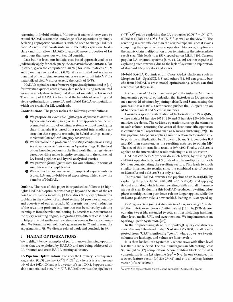
Encoding into a Relational Model. Let E be an LA expression
(query) and V be a set of materialized views. We reduce the LA
views-based rewriting problem to the relational rewriting problem
under integrity constraints, as follows (see Figure 1). First, we encode
relationally E,V, and the set Lops of LA operators. Note that the
relations used in the encoding are virtual and hidden, i.e., invisibleto both the application designers and users. They only serve to
support query rewriting via relational techniques.
These virtual relations are accompanied by a set of relational
integrity constraints encLA(LAprop ) that reflect a set LAprop of LA
properties of the supported Lops operations. For instance, we model
the matrix addition operation using a relation addM (M,N ,R), de-noting thatR is the result ofM+N , together with a set of constraints
stating that addM is a functional relation that is commutative, asso-ciative, etc. These constraints are Tuple Generating Dependencies
(TGDs) or Equality Generating Dependencies (EGDs) [15], whichare a generalization of key and foreign key dependencies. We detail
our relational encoding in §5.
Reduction fromLA-based to Relational Rewriting. Our reduc-tion translates the declaration of each view V ∈ V to constraints
encLA(V ) that reflect the correspondence between V ’s input dataand its output. Separately, E is also encoded as a relational query
encLA(E) over the relational encodings of Lops and its matrices.
The reformulation problem is reduced to a purely relational
setting as follows. We are given a (purely LA or hybrid) query
expression E ∈ L and a set V ⊆ L of hybrid views. We encode
E as the relational query encLA(E), the views as the relational in-tegrity constraints CV = encLA(V1) ∪ . . . ∪ encLA(Vn ). We add as
further input the set of relational constraints encLA(LAprop ) men-
tioned above, which specify properties of the LA operators. We
call them Matrix-Model encoding Constraints, or MMC in short.
We must find a rewriting RWe expressed over the relational views
CV , such that RWe is equivalent to encLA(E) under the constraints(CV
⋃MMC) and is optimal according to our cost model. Note
that RWe is a relationally encoded rewriting of E; a final decodingstep is needed to obtain E ′ ∈ L, the (LA or hybrid) rewriting of E.
The challenge in coming upwith the reduction consists in design-
ing an encoding, i.e., one in which rewritings found by (i) encodingrelationally, (ii) solving the resulting relational rewriting problem,
and (iii) decoding a resulting rewriting over the views, is guaran-teed to produce an equivalent expression E ′ (see §5).
Relational RewritingUsingConstraints. To solve the relationalrewriting problem under constraints, the engine of choice is Prove-
nance Aware Chase&Backchase (PACB) [30]. The PACB engine
(PACB++ hereafter) has been extended to utilize the Prunedprovalgorithm discussed in [29, 30], which prunes inefficient rewritings
during the search phase, based on a simple cost model (see §6).
Decoding of the Relational Rewriting. For the selected rela-
tional reformulation RWe by PACB++, a decoding step dec(RWe ) is
performed to translate RWe into the native syntax of its respective
underlying store/engine (e.g., R, DML, etc.).
5 REDUCTION TO THE RELATIONAL MODELOur internal model is relational, and it makes prominent use of
expressive integrity constraints. This framework suffices to describe
the features and properties of most data models used today, notably
including relational, XML, JSON, graph, etc [16, 17].
Going beyond, in this section, we present a novel way to reasonrelationally about LA operations by treating them as un-interpreted
functions with black-box semantics, and adding constraints that
capture their important properties. First, we give an overview of a
wide range of LA operations that we consider (§5.1). Then, in §5.2,
we show how matrices and their operations can be encoded usinga set of virtual relations, part of a schema we call VREM (for
Virtual Relational Encoding of Matrices), together with the integrity
constraints MMC that capture the properties of these operations.
§5.3 exemplifies relational rewritings obtained via our reduction.
5.1 Matrix AlgebraWe consider a wide range of matrix operations [19, 37], which are
common in real-world ML algorithms [4]: element-wise multipli-
cation (multiE ), matrix-scalar multiplication (multiMS ), matrix
multiplication (multiM ), addition (addM ), division (divM ), trans-
position (tr), inversion (invM ), determinant (det), trace (trace), di-agonal (diag), exponential (exp), adjoints (adj), direct sum (sumD ),direct product (productD ), summation (sum), rows/columns sum-
mation (rowSums, colSums, respectively), QR (QR), Cholesky (CHO),LU (LU), and pivoted LU (LUP) decompositions.
5.2 VREM Schema and Relational EncodingTo model LA operations on the VREM relational schema (part
of which appears in Table 1), we also rely on a set of integrity
constraintsMMC, which are encoded using relations inVREM.
We detail the encoding below.
5.2.1 Base Matrices and Dimensionality Modeling. We de-
note by Mk×z (D) a matrix of k rows and z columns, whose values
come from a domain D, e.g., the domain of real numbers R. Forbrevity we just use Mk×z . We define a virtual relation name(M,n) ∈VREM attaching a unique ID M to any matrix identified by a
name denoted n (which may be e.g., of the form “/M.csv”). This rela-
tion (shown at the top left in Table 1) is accompanied by an EGD key
constraint Iname ∈ MMCm , whereMMCm ⊂ MMC, statingthat two matrices with the same name n have the same ID:
Iname : ∀M∀N name(M,n) ∧ name(N ,n) → M = N
Note that thematrix ID inname (and all the other virtual relationsused in our encoding) are not IDs of individualmatrix objects: rather,
each identifies an equivalence class (induced by value equality) of
expressions. That is, two expressions are assigned the same ID iff
they yield value-based-equal matrices. In Table 1, we useM and Nto denote input matrices’ IDs, R for the resulting matrix ID, and sfor scalar input and output.
The dimensions of a matrix are captured by a size(M,k, z) rela-tion, where k and z are the number of rows, resp. columns andMis an ID. An EGD constraint Isize ∈ MMCm holds on the sizerelation, stating that the ID determines the dimensions:
Isize : ∀M∀k1∀z1∀k2∀z2size(M,k1, z1) ∧ size(M,k2, z2) → k1 = k2 ∧ z1 = z2
The identity and zero matrices are captured by Zero(O) andIdentity(I ) relations, where O and I denote their IDs, respectively.They are accompanied by EGD constraintsIiden ,Izero ∈ MMCm ,
stating that zero matrices with the same sizes have the same IDs,
and this also applies for identity matrices with the same size:
Izero : ∀O1∀O2∀k∀zZero(O1) ∧ size(O1,k, z) ∧ Zero(O2) ∧ size(O2,k, z) → O1 = O2
Iiden : ∀I1∀I2Identity(I1) ∧ size(I1,k,k) ∧ Identity(I2) ∧ size(I2,k,k) → I1 = I2
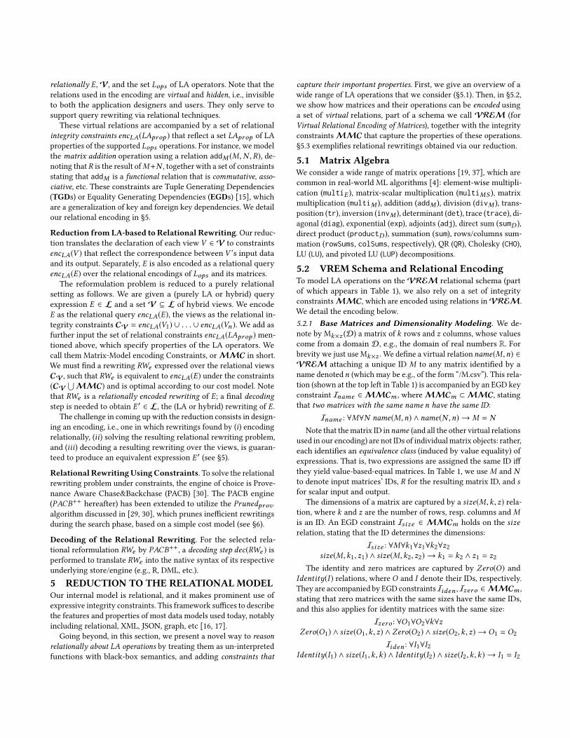
Operation Encoding Operation Encoding Operation EncodingMatrix scan name(M,n) Inversion invM (M,R) Cells sum sum(M, s)
Multiplication multiM (M,N ,R)Scalar
Multiplication
multiMS (s,M,R) Row sum rowSums(M,R)
Addition addM (M,N ,R) Determinant det(M,R) Colsums colSums(M,R)
Division divM (M,N ,R) Trace trace(M, s) Direct sum sumD (M,N ,R)
Hadamard
product
multiE (M,N ,R) Exponential exp(M,R) Direct product productD (M,N ,R)
Transposition tr(M,R) Adjoints adj(M,R) Diagonal diag(M,R)
Table 1: Snippet of theVREM Schema
5.2.2 Encoding Matrix Algebra Expressions. LA operations
are encoded into dedicated relations, as shown in Table 1. We now
illustrate the encoding of an LA expression on theVREM schema.
Example 5.1. Consider the LA expression E: ((MN )T ), where thetwo matrices M100×1 and N1×10 are stored as “M .csv” and “N .csv”,respectively. The encoding function encLA(E) takes as argument theLA expression E and returns a conjunctive query whose: (i) body isthe relational encoding of E usingVREM (see below), and (ii) headhas one distinguished variable, denoting the equivalence class of theresult. For instance:
enc(((MN )T ) =Let enc(MN ) =
Let enc(M) = Q0(M):- name(M, “M .csv”);enc(N ) = Q1(N ):- name(N , “N .csv”);R1 = freshId()
inQ2(R1):- multiM (M,N ,R1)∧Q0(M)∧ Q1(N );
R2 = freshId()in
Q(R2):- tr(R1,R2)∧ Q2(R1);
In the above, nesting is dictated by the syntax of E. From the inner(most indented) to the outer, we first encodeM and N as small queriesusing the name relation, then their product (to whom we assign thenewly created identifier R1 ), using themultiM relation and encodingthe relationship between this product and its inputs in the definitionof Q2(R1). Next, we create a fresh ID R2 used to encode the full E(the transposed of Q2) via relation tr, in Q(R2). For brevity, we omitthe matrices’ size relations in this example and hereafter. UnfoldingQ2(R1) in the body of Q yields:
Q(R2) :- tr(R1,R2)∧ multiM (M,N ,R1)∧Q0(M)∧Q1(N );
Now, by unfolding Q0 and Q1 in Q, we obtain the final encoding of((MN )T ) as a conjunctive query Q:
Q(R2) :- tr(R1,R2)∧ multiM (M,N ,R1)∧name(M, “M .csv”)∧name(N , “N .csv”);
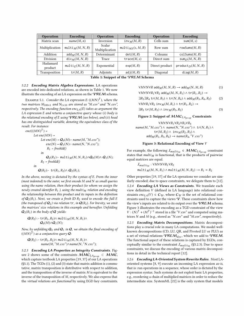
5.2.3 Encoding LA Properties as Integrity Constraints. Fig-ure 2 shows some of the constraints MMCLAprop ⊂ MMC,which capture textbook LA properties [19, 37] of our LA operations
(§5.1). The TGDs (1), (2) and (3) state that matrix addition is commu-
tative, matrix transposition is distributive with respect to addition,
and the transposition of the inverse of matrixM is equivalent to the
inverse of the transposition ofM , respectively. We also express that
the virtual relations are functional by using EGD key constraints.
∀M∀N∀R addM (M,N ,R) → addM (N ,M,R) (1)
∀M∀N∀R1∀R2 addM (M,N ,R1) ∧ tr(R1,R2) →
∃R3∃R4 tr(M,R3) ∧ tr(N ,R4) ∧ addM (R3,R4,R2) (2)
∀M∀R1∀R2 invM (M,R1) ∧ tr(R1,R2) →
∃R3 tr(M,R3) ∧ invM (R3,R2) (3)
Figure 2: Snippet ofMMCLAprop Constraints
∀M∀N∀R1∀R2∀R3∀R4name(M, “M .csv”) ∧ name(N , “N .csv”) ∧ tr(N ,R1) ∧
tr(M,R2) ∧ invM (R2,R3) ∧addM (R1,R3,R4) → name(R4, “V .csv”)
Figure 3: Relational Encoding of View V
For example, the following ImultiM ∈ MMCLAprop constraint
states thatmultiM is functional, that is the products of pairwise
equal matrices are equal.
ImultiM : ∀M∀N∀R1∀R2multiM (M,N ,R1) ∧ multiM (M,N ,R2) → R1 = R2
Other properties [19, 37] of the LA operations we consider are sim-
ilarly encoded; due to space constraints, we delegate them to [12].
5.2.4 Encoding LA Views as Constraints. We translate each
view definition V (defined in LA language) into relational con-
straints encLA(V ) ∈ CV , where CV is the set of relational con-
straints used to capture the views V. These constraints show how
the view’s inputs are related to its output over theVREM schema.
Figure 3 illustrates the encoding as a TGD constraint of the view
V : (N )T + (MT )−1 stored in a file “V .csv” and computed using ma-
trices N andM (e.g., stored as “N .csv” and “M .csv”, respectively).
5.2.5 Encoding Matrix Decompositions. Matrix decomposi-
tions play a crucial role in many LA computations. We model well-
known decompositions (CD, LU, QR, and Pivoted LU or PLU) as
a set of virtual relations VREMdec , which we add to VREM.
The functional aspect of these relations is captured by EGDs, con-
ceptually similar to the constraint ImultiM (§5.2.3). Due to space
constraints, we discuss the encoding of various matrix decomposi-
tions in detail in the technical report [12].
5.2.6 EncodingLA-Oriented SystemRewriteRules. Most LA-
oriented systems [8, 9] execute an incoming LA expression as-is,that is: run operations in a sequence, whose order is dictated by the
expression syntax. Such systems do not exploit basic LA properties,
e.g., reordering a chain of multiplied matrices in order to reduce the
intermediate size. SystemML [22] is the only system that models
some LA properties as static rewrite rules. It also comprises a set
of rewrite rules which modify the given expressions to avoid large
intermediates for aggregation and statistical operations such as
rowSums(M), sum(M), etc. For example, SystemML uses rule:
sum(MN ) = sum(colSums(M)T ⊙ rowSums(N )) (i)
to rewrite sum(MN ) (summing all cells in the matrix product) where
⊙ is a matrix element-wise multiplication, to avoid actually com-
putingMN and materializing it. However, the performance benefits
of rewriting depend on the rewriting power (or, in other words,
on how much the system understands the semantics of the incomingexpression), as the following example shows.
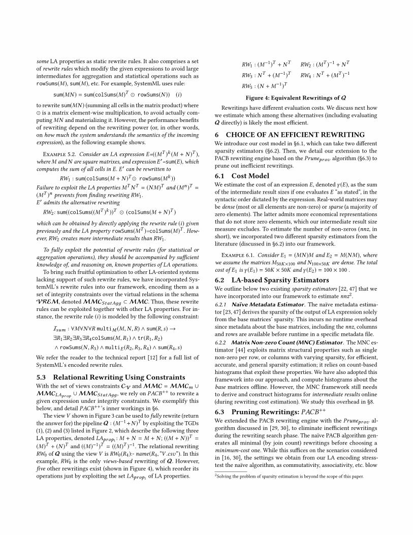
Example 5.2. Consider an LA expression E=((MT )k (M + N )T ),whereM andN are square matrixes, and expression E ′=sum(E), whichcomputes the sum of all cells in E. E ′ can be rewritten to
RW1 : sum(colSums(M + N )T ⊙ rowSums(Mk ))
Failure to exploit the LA propertiesMTNT = (NM)T and (Mn )T =
(MT )n prevents from finding rewriting RW1.E ′ admits the alternative rewriting
RW2: sum((colSums((MT )k ))T ⊙ (colSums(M + N )T )
which can be obtained by directly applying the rewrite rule (i) givenpreviously and the LA property rowSums(MT )=colSums(M)T . How-ever, RW2 creates more intermediate results than RW1.
To fully exploit the potential of rewrite rules (for statistical oraggregation operations), they should be accompanied by sufficientknowledge of, and reasoning on, known properties of LA operations.
To bring such fruitful optimization to other LA-oriented systems
lacking support of such rewrite rules, we have incorporated Sys-
temML’s rewrite rules into our framework, encoding them as a
set of integrity constraints over the virtual relations in the schema
VREM, denotedMMCStatAдд ⊂ MMC. Thus, these rewriterules can be exploited together with other LA properties. For in-
stance, the rewrite rule (i) is modeled by the following constraint:
Isum : ∀M∀N∀R multiM (M,N ,R) ∧ sum(R, s) →
∃R1∃R2∃R3∃R4colSums(M,R1) ∧ tr(R1,R2)
∧ rowSums(N ,R3) ∧ multiE (R2,R3,R4) ∧ sum(R4, s)
We refer the reader to the technical report [12] for a full list of
SystemML’s encoded rewrite rules.
5.3 Relational Rewriting Using ConstraintsWith the set of views constraints CV and MMC =MMCm ∪
MMCLAprop ∪MMCStatAдд , we rely on PACB++ to rewrite a
given expression under integrity constraints. We exemplify this
below, and detail PACB++’s inner workings in §6.
The viewV shown in Figure 3 can be used to fully rewrite (returnthe answer for) the pipelineQ : (M−1+N )T by exploiting the TGDs
(1), (2) and (3) listed in Figure 2, which describe the following three
LA properties, denoted LAprop1 : M + N = M + N ; ((M + N ))T =
(M)T + (N )T and ((M)−1)T = ((M)T )−1. The relational rewriting
RW0 of Q using the view V is RW0(R4):- name(R4, “V .csv”). In this
example, RW0 is the only views-based rewriting of Q. However,
five other rewritings exist (shown in Figure 4), which reorder its
operations just by exploiting the set LAprop1 of LA properties.
RW1 : (M−1)T + NT RW2 : (M
T )−1 + NT
RW3 : NT + (M−1)T RW4 : N
T + (MT )−1
RW5 : (N +M−1)T
Figure 4: Equivalent Rewritings of QRewritings have different evaluation costs. We discuss next how
we estimate which among these alternatives (including evaluating
Q directly) is likely the most efficient.
6 CHOICE OF AN EFFICIENT REWRITINGWe introduce our cost model in §6.1, which can take two different
sparsity estimators (§6.2). Then, we detail our extension to the
PACB rewriting engine based on the Pruneprov algorithm (§6.3) to
prune out inefficient rewritings.
6.1 Cost ModelWe estimate the cost of an expression E, denoted γ (E), as the sumof the intermediate result sizes if one evaluates E “as stated”, in the
syntactic order dictated by the expression. Real-world matrices may
be dense (most or all elements are non-zero) or sparse (a majority of
zero elements). The latter admits more economical representations
that do not store zero elements, which our intermediate result size
measure excludes. To estimate the number of non-zeros (nnz, inshort), we incorporated two different sparsity estimators from the
literature (discussed in §6.2) into our framework.
Example 6.1. Consider E1 = (MN )M and E2 = M(NM), wherewe assume the matricesM50K×100 and N100×50K are dense. The totalcost of E1 is γ (E1) = 50K × 50K and γ (E2) = 100 × 100 .
6.2 LA-based Sparsity EstimatorsWe outline below two existing sparsity estimators [22, 47] that wehave incorporated into our framework to estimate nnz2.6.2.1 Naïve Metadata Estimator. The naïve metadata estima-
tor [23, 47] derives the sparsity of the output of LA expression solely
from the base matrices’ sparsity. This incurs no runtime overhead
since metadata about the base matrices, including the nnz, columns
and rows are available before runtime in a specific metadata file.
6.2.2 Matrix Non-zero Count (MNC) Estimator. TheMNC es-
timator [44] exploits matrix structural properties such as single
non-zero per row, or columns with varying sparsity, for efficient,
accurate, and general sparsity estimation; it relies on count-based
histograms that exploit these properties. We have also adopted this
framework into our approach, and compute histograms about the
base matrices offline. However, the MNC framework still needs
to derive and construct histograms for intermediate results online(during rewriting cost estimation). We study this overhead in §8.
6.3 Pruning Rewritings: PACB++We extended the PACB rewriting engine with the Pruneprov al-
gorithm discussed in [29, 30], to eliminate inefficient rewritings
during the rewriting search phase. The naïve PACB algorithm gen-
erates all minimal (by join count) rewritings before choosing a
minimum-cost one. While this suffices on the scenarios considered
in [16, 30], the settings we obtain from our LA encoding stress-
test the naïve algorithm, as commutativity, associativity, etc. blow
2Solving the problem of sparsity estimation is beyond the scope of this paper.
up the space of alternate rewritings exponentially. Scalability con-
siderations forced us to further optimize naïve PACB to find only
minimum-cost rewritings, aggressively pruning the others during
the generation phase. We detail below just enough of the PACB’sinner working to explain Pruneprov .
6.3.1 PACB Background. At the core of PACB is the idea to
model views as constraints, in this way reducing the view-based
rewriting problem to constraints-only rewriting. Specifically, for
a given view V defined by a query, the constraint VIO states that
for every match of the view body against the input data, there is acorresponding (head) tuple in the view output, while the constraintVOI states the converse inclusion, i.e., each view output tuple is due toa view bodymatch. From a setV of view definitions, PACB therefore
derives a set of view constraints CV = {VIO ,VOI | V ∈ V}.
Given a source schema σ with a set of integrity constraints I,
a set V of views defined over σ , and a conjunctive query Q over
σ , the rewriting problem thus becomes: find every reformulation
query ρ over the schema of view namesV that is equivalent to Qunder the constraints I ∪CV .
Example 6.2. For instance, if σ = {R, S}, I = ∅, τ = {V }
and we have a view V materializing the join of relations R and S ,V (x ,y):- R(x , z) ∧ S(z,y), the pair of constraints capturing V is thefollowing:
VIO : ∀x∀z∀y R(x , z) ∧ S(z,y) → V (x ,y)
VOI : ∀x∀yV (x ,y) → ∃z R(x , z) ∧ S(z,y).
Given the queryQ(x ,y):- R(x , z)∧S(z,y), PACB finds the rewritingRW (x ,y):- V (x ,y). Algorithmically, this is achieved by:
(i) chasingQ with the constraintsI∪C IOV
, whereC IOV= {VIO |V ∈
V}; intuitively, this enriches (extends) Q with all the consequencesthat follow from its atoms and the constraints I ∪C IO
V.
(ii) restricting the chase result to only the V-atoms; the result iscalled the universal planU .
(iii) annotating each atom of the universal planU with a uniqueID called a provenance term.
(iv) chasing U with the constraints in I ∪ COIV
, where COIV=
{VOI | V ∈ V}, and annotating each relational atom a introduced bythese chase steps with a provenance formula
3 π (a), which gives theset ofU -subqueries whose chasing led to the creation of a; the resultof this phase, called the backchase, is denoted B.
(v) matching Q against B and outputting as rewritings the subsetsofU that are responsible for the introduction (during the backchase)of the atoms in the image h(Q) of Q ; these rewritings are read offdirectly from the provenance formula π (h(Q)).
In our example, I is empty, C IOV= {VIO }, and the result of the
chase in phase (i) is Q1(x ,y):- R(x , z) ∧ S(z,y) ∧ V (x ,y). The uni-versal plan obtained in (ii) by restricting Q1 to the schema of viewnames is U (x ,y):- V (x ,y)p0 , where p0 denotes the provenance termof atom V (x ,y). The result of backchasing U with COI
Vin phase (iv)
is B(x ,y):- V (x ,y)p0∧ R(x , z)p0 ∧ S(z,y)p0 . Note that the π (R) andπ (S) of the R and S atoms (a simple term p0, in this example) areintroduced by chasing the view V . Finally, in phase (v) we find onematch image given by h from Q’s body into the R and S atoms from
3Provenance formulas are constructed from provenance terms using logical conjunc-
tion and disjunction.
B’s body. The provenance π (h(Q)) of the image of Q under h is p0,which corresponds to an equivalent rewriting: RW (x ,y):- V (x ,y).
6.3.2 Pruneprov Minimum-Cost Rewriting . Recall from §6.3.1
that theminimal rewritings of a queryQ are obtained by first finding
the setH of all matches (i.e., containment mappings) fromQ to the
result B of backchasing the universal planU . Denoting with π (S)the provenance formula of a set of atoms S , PACB computes the
DNF form D of
∨h∈H π (h(Q)). Each conjunct c of D determines a
subquery sq(c) ofU which is guaranteed to be a rewriting of Q .The idea behind cost-based pruning is that, whenever the naïve
PACB backchase would add a provenance conjunct c to an exist-
ing atom a’s provenance formula π (a), Pruneprov does so more
conservatively: if the cost γ (sq(c)) is larger than the minimum cost
thresholdT found so far, then c will never participate in a minimum-
cost rewriting and need not be added to π (a). Moreover, atom aitself need not be chased into B in the first place if all its provenance
conjuncts have above-threshold cost.
Example 6.3. Let E = M(NM), where we assume for simplicitythatM50K×100 and N100×50K are dense. Exploiting the associativityof matrix-multiplication (MN )M = M(NM) during the chase leadsto the following universal planU annotated with provenance terms:
U (R2) : name(M, “M .csv”)p0 ∧ size(M, “50000”, “100”)p1 ∧name(N , “N .csv”)p2 ∧ size(N , “100”, “50000”)p3∧multiM (M,N ,R1)
p4∧ multiM (R1,M,R2)p5∧
multiM (N ,M,R3)p6∧ multiM (M,R3,R2)
p7
Now, consider in the backchase the associativity constraint C :∀M∀N∀R1∀R2multiM (M,N ,R1) ∧ multiM (R1,M,R2) →
∃R4multiM (N ,M,R4) ∧ multiM (M,R4,R2)
There exists a match h embedding the two atoms in the premise P ofC into theU atoms whose provenance annotations are p4 and p5. Theprovenance conjunct collected from P ’s image is π (h(P))=p4 ∧ p5.
Without pruning, the backchase would chaseU with the constraintC , yieldingU ′ which features additional π (h(P))-annotated atoms
multiM (N ,M,R4)p4∧p5∧ multiM (M,R4,R2)
p4∧p5
E has precisely two matches h1,h2 into U ′. h1(E) involves thenewly added atoms as well as those annotated with p0,p1,p2,p3.Collecting all their provenance annotations yields the conjunct c1 =p0 ∧ p1 ∧ p2 ∧ p3 ∧ p4 ∧ p5. c1 determines the U -subquery sq(c1)corresponding to the rewriting (MN )M , of cost (50K)2.
h2(E)’s image yields the provenance conjunct c2 = p0 ∧ p1 ∧ p2 ∧p3 ∧ p6 ∧ p7, which determines the rewritingM(NM) that happensto be the original expression E of cost 1002.
The naïve PACB would find both rewritings, cost them, and drop theformer ,which introduces a large intermediate result (γ (sq(π (h(P))) =(50K)2), above the threshold, in favor of the latter.
With pruning, the threshold T is the cost of the original expres-sion 100
2. The chase step with C is never applied, as it would intro-duce the provenance conjunct π (h(P)) which determines U-subquerysq(π (h(P)) = multiM (M,N ,R1)
p4 ∧ multiM (R1,M,R2)p5
of cost (50K)2 exceeding T . The atoms needed as image of E underh1 are thus never produced while backchasing U , so the expensiverewriting is never discovered. This leaves only the match image h2(E),which corresponds to the efficient rewritingM(NM).
6.3.3 Our improvements on Pruneprov . Whenever the pruned
chase step is applicable and applied for each constraint, the orig-
inal algorithm searches for all minimal-rewritings RW that can
be found “so far”, then it costs each rw ∈ RW to find the “so far”
minimum-cost one rwe and adjusts the thresholdT to the cost of rwe .
However, this strategy can cause redundant costing of rw ∈ RWwhenever the pruned chase step is applied again for another con-
straint. Therefore, in our modified version of Pruneprov , we keeptrack of the rewriting costs already estimated, to prevent such re-
dundant work. Additionally, the search for minimal-rewritings “sofar” (matches of the query Q into the evolving universal plan in-
stanceU ′, see §6.3.1), whenever the pruned chase step is applied, is
modeled as a query evaluation ofQ againstU ′(viewed as a symbol-
ic/canonical database [15]). This involves repeatedly evaluating the
same query plan. However, the query is evaluated over evolutions
of the same instance. Each pruned chase step adds a few new tuplesto the evolving instance, corresponding to atoms introduced by that
step, while most of the instance is unchanged. Therefore, instead
of evaluating the query plan from scratch, we employ incremental
evaluation as in [30]. The plan is kept in memory along with the
populated hash tables and, whenever new tuples are added to the
evolving instance, we push them to the plan.
7 GUARANTEES ON THE REDUCTIONWe detail the conditions under which we guarantee that our ap-
proach is sound (i.e., generates only equivalent, cost-optimal rewrit-
ings), and complete (i.e., finds all equivalent cost-optimal rewritings).
Let V ⊆ L be a set of materialized view definitions, where L is
the language of hybrid expressions described in §3.
Let LAprop be a set of properties of the LA operations in Lopsthat admits relational encoding overVREM. We say that LApropis terminating if it corresponds to a set of TGDs and EGDs with
terminating chase (this holds for our choice of LAprop ).Denote with γ a cost model for expressions from L. We say that
γ is monotonic if expressions are never assigned a lower cost than
their subexpressions (this is true for both models we used).
We call E ∈ L (γ ,LAprop ,V)-optimal if for every E ′ ∈ L that
is (LAprop ,V)-equivalent to E we have γ (E ′) ≥ γ (E).Let Eq
γ ⟨LAprop ,V⟩(E) denote the set of all (γ ,LAprop ,V)-opti-
mal expressions that are (LAprop ,V)-equivalent to E.We denote with HADAD⟨LAprop ,V,γ ⟩ our parameterized so-
lution based on relational encoding followed by PACB++ rewrit-
ing and next by decoding all the relational rewritings generated
by the cost-based pruning PACB++ (recall Figure 1). Given E ∈
L, HADAD⟨LAprop ,V,γ ⟩(E) denotes all expressions returned by
HADAD⟨LAprop ,V,γ ⟩ on input E.
Theorem 7.1 (Soundness). If the cost model γ is monotonic, thenfor every E ∈ L and every rw ∈ HADAD⟨LAprop ,V,γ ⟩(E), we haverw ∈ Eqγ ⟨LAprop ,V⟩(E).
Theorem 7.2 (Completeness). If γ is monotonic and LAprop isterminating, then for everyE ∈ L and every rw ∈ Eqγ ⟨LAprop ,V⟩(E),we have rw ∈ HADAD⟨LAprop ,V,γ ⟩(E).
8 EXPERIMENTAL EVALUATIONWe evaluate HADAD to answer the following questions:
• §8.1.1, §8.1.2, §8.2.1 and §8.2.2: Can HADAD find rewrites
with/without views that outperform the original pipelines
without modifying the internals of the existing systems? Are
the identified rewrites found by state-of-the-art platforms?
• §8.1.3 : Is HADAD’s optimization overhead compensated by
the performance gains in execution?
We evaluate our approach, first on pure LA pipelines (§8.1), thenon hybrid expressions (§8.2). Due to space constraints, we high-
light some of our results here, relegating the full details to [12].
Experimental Environment.We used a single node with an In-
tel(R) Xeon(R) CPU E5-2640 v4 @ 2.40GHz, and 123G RAM. We run
on OpenJDK Java 8 VM. As for LA systems/libraries, we used
R 3.6.0, Numpy 1.16.6 (python 2.7), TensorFlow r1.4.2, Spark2.4.5 (MLlib), and SystemML 1.2.0. For hybrid experiments, we
use MorpheusR[5] and SparkSQL [18].
Systems Configuration Tuning. We use a JVM-based linear al-
gebra library for SystemML as recommended in [46], at the opti-
mization level 4. Additionally, we enable multi-threaded matrix
operations in a single node. We run Spark in a single node setting
using OpenBLAS (built from the sources as detailed in [6]) to take
advantage of its accelerations [46]. SparkMLlib’s datatypes do not
support many basic LA operations, such as Hadamard-product, To
support them, we use the Breeze Scala library [2], convert MLlib’s
datatypes to Breeze types and express the basic LA operations in
Spark. The driver memory allocated for Spark and SystemML is
115GB. To maximize TensorFlow performance, we compile it from
sources. For all systems/libraries, we set the number of cores to 24and use double-precision numbers.
8.1 LA-based ExperimentsIn these experiments, we study the performance benefits of our ap-
proach on LA-based pipelines as well as our optimization overhead.
Datasets.We use four real-world, sparse matrices. We present
two of them here and describe the others in [12]. We use an Amazon
books review [1](in JSON) and a Netflix movie rating datasets [7].
The two were converted into matrices where columns are items
and rows are customers [47]. We extract subsets of them to ensure
various computations applied on them fit in memory (e.g., NS de-
notes the small version of the Netflix dataset and AL denotes the
large version for Amazon). We also use a set of synthetic, densematrices; their dimensions appear at the top of experiment figures.
LA benchmark. We select a set P of 57 LA pipelines used in
prior studies and/or frequently occurring in real-world LA compu-
tations, as follows:
• Real-world pipelines (10) include expressions used in ALS(P1.7) [39], Ordinary Least Squares Regression (OLS) [46]
(P1.6) and matrix chain multiplication (P1.3 and P1.5). Others
are detailed in [12].
• Synthetic pipelines (47) were also generated, based on a
set of basic matrix operations (inverse, multiplication, addi-
tion, etc.), and a set of combination templates, written as a
Rule-Iterated Context-Free Grammar (RI-CFG) [41].
Table 2 lists pipelines that we discus here. All 57 benchmark pipelines
appear in [12] (§9.1, Tables 2 and 3).

0.001
0.01
0.1
1
10
100
SM R NP TF SP
TotalExecutionTimeLogscale-[s]
M:50Kx100, N:100x50KQexec RWexec RWfnd
X
(a) P1.1
0.001
0.01
0.1
1
SM R SPTotalExecutionTime-[s]
A:AL1(1Mx100), B:1Mx100
(b) P1.2
0.001
0.01
0.1
1
10
SM R SP
M:NS(50Kx100), N:100x50K
(c) P1.3
0.001
0.01
0.1
1
10
SM R NP TF SP
M:50Kx100, N:100x50K
X
(d) P1.4
Figure 5: P1.1, P1.2, P1.3, and P1.4 Evaluation Before and After Rewriting
Figure 6: R speed-up on P¬Opt
No. Expression No. ExpressionP1.1 (MN )T P1.2 (A + B)v1
P1.3 (MN )M P1.4 sum(rowSums(NTMT ))
P1.5 ((MN )M )N P1.6 (DTD)−1(DTv1)
P1.7 (uvT − X )v P1.8 ((((C + D)T )−1)D)C
Table 2: Subset of LA Benchmark Pipelines
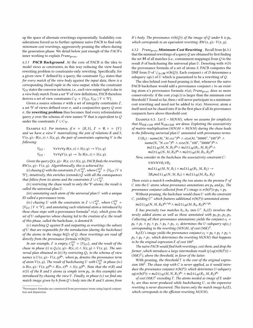
Methodology. In §8.1.1, we show the performance benefits of
HADAD to LA systems/tools mentioned above using a setP¬Opt ⊂
P of 38 pipelines. The performance of P¬Optcan be improved just
by exploiting LA properties (in the absence of views). For TensorFlowand NumPy, we present the results only for dense matrices, due to
limited support for sparse matrices. In §8.1.2, we show how our ap-
proach improves the performance of 30 pipelines from P, denoted
PV iews, using pre-materialized views. Finally, in §8.1.3, we study
our rewriting performance and optimization overhead for the set
POpt = P \ P¬Optof 19 pipelines that are already optimized.
8.1.1 Effectiveness of LA Rewriting (No Views). For each sys-tem, we run the original pipeline and our rewriting 5 times; we
report the average of the last 4 running times. We exclude the data
loading time. For fairness, we ensured SparkMLib and SystemML
compute the entire pipeline (despite their lazy evaluation mode).
Figure 5 illustrates the original pipeline execution time Qexecand the selected rewriting execution time RWexec for P1.1, P1.2,P1.3, and P1.4, including the rewriting time RWf ind , using the
MNC cost model from §6.2.2. For each pipeline, the used datasets
are on top of the figure. For brevity in the figures, we use SM for
SystemML, NP for NumPy, TF for Tensorflow, and SP for MLlib.
For P1.1 (see Figure 5(a)), both matrices are dense. The speed-up
(1.3× to 4×) comes from rewriting (MN )T (intermediate result size
is (50K)2) into NTMT, much cheaper since both NT
and MTare
of size 50K × 100. We exclude MLlib from this experiment since it
failed to allocate memory for the intermediate matrix (Spark/MLLib
limits the maximum size of a dense matrix). As a variation (not
plotted in the Figure), we ran the same pipeline with the ultra-
sparse Amazon AS : 50K × 100 matrix (0.0075% nnz) used as M .
TheQexec and RWexec time are very comparable using SystemML,
because we avoid dense intermediates and multiplication becomes
efficient. In R, this scenario leads to a runtime exception and to
avoid it, we cast M during load time to a dense matrix. Thus, the
speed-up achieved is the same as if M and N were both dense. If,
instead, NS : 50K × 100 (1.3911% non-zeros) plays the role of M ,
our rewrite achieves ≈ 1.8× speed-up for SystemML.
For P1.2 (Figure 5(b)), we rewrite (A+B)v1 toAv1+Bv1. AddingAmazon sparse matrix AL1 (0.0065% nnz) used as A to a dense
matrix B results into materializing a dense intermediate of size
1M × 100. Instead, Av1 + Bv1 has fewer nnz in the intermediate
results, and Av1 can be computed efficiently since A is sparse. The
MNC sparsity estimator has a noticeable overhead. We run the
same pipeline, where the dense 5M × 100 matrix plays both A and
B (not shown in the Figure). This leads to speed-up of up to 9× for
MLlib, which does not natively support matrix addition, thus we
convert its matrices to Breeze types in order to perform it [46].
The intermediate matrix size for evaluation plan (MN )M of P1.3(Figure 5(c)) is (50K)2, but only 100
2for its rewritingM(NM). To
avoid MLLib memory failure, we use BlockMatrix type for both
matrices. While M thus converted has the same sparsity, Spark
views it as being of a dense type (multiplication on BlockMatrix
produces dense matrices) [11]. SystemML does optimize the chain
order if the user does not enforce it. Further (not shown in the
Figure), we ran P1.3 with AS in the role of M . This is 4× faster
in SystemML since with an ultra sparseM , multiplication is more
efficient. This is not the case for MLlib which views it as dense. For
R, we again had to densifyM during loading to prevent crashes.
Figure 5(d) shows speedups of up to 42× when rewriting P1.4into sum((colSums(M))T ⊙rowSums(N )). This exploits several prop-
erties:
(i) (MN )T = NTMT ,
(ii) sum(MT ) =sum(M),
(iii) sum(rowSums-(M)) = sum(M), and
(iv) sum(MN )=sum((colSums(M))T ⊙ rowSums-(N )).
SystemML captures (ii), (iii), and (iv) as rewrite rules, however,it is unable to exploit them here since it is unaware of (i). Othersystems do not exploit these properties.
0.001
0.01
0.1
1
10
100
SM R SP
TotalExecutionTimeLogscale-[s]
M:NS(50Kx100), N:100x50KQexec RWexec RWfnd
(a) P1.5
0.001
0.01
0.1
1
10
100
SM R NP TF SP
C:10Kx10K, D:10Kx10K
0.001
0.01
0.1
1
10
100
SM R NP TF SP
C:10Kx10K, D:10Kx10K
X
(b) P1.6
0.001
0.01
0.1
1
10
100
1000
SM R SP
X:AL2(100Kx50K), u:100Kx1, v:50Kx1
X
(c) P1.7
0.001
0.01
0.1
1
10
100
SM R NP TF SP
C:10Kx10K, D:10Kx10K
X
(d) P1.8
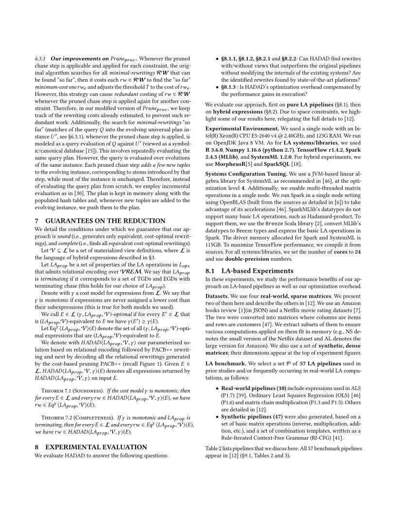
Figure 7: P1.5, P1.6, P1.7 and P1.8 Evaluation Before and After Rewriting Using the Views Vexp
Speed-up Summary. Figure 6 shows the distribution of the signif-
icant rewriting speed-up on P¬Optrunning on R (other systems’
results are in [12]) , and using the MNC-based cost model. For clar-
ity, we split the distribution into two figures: on the left, 25 P¬Opt
pipelines with speed-up lower than 10×; on the right, the remaining
13 with greater speed-up. Among the former, 87% achieved at least
1.5× speed-up. The latter are sped up by 10× to 60×. The ((D)−1)−1
pipeline is an extreme case here (not plotted): it is sped up by about
1000×, simply by rewriting ((D)−1)−1 into D (which R fails to do).
8.1.2 Effectiveness of view-based LA rewriting. We have de-
fined a set Vexp of 12 views that pre-compute the result of some
expensive operations (multiplication, inverse, determinant, etc.)
which can be used to answer our PV iewspipelines, and material-
ized them on disk as CSV files. The experiments outlined below
used the naïve cost model; all graphs have a log-scale y axis.
For P1.5 (Figure 7(a)), using the viewV4 = NM and the multipli-
cation associativity leads to up to 2.8× speed-up. Figure 7(b) shows
the performance gain for OLS pipeline P1.6, discussed in (§2). This
rewrite leads to up to 150× speed-up on MLlib. On SystemML, the
original pipeline timed out (> 1000 seconds).
P1.7 (Figure 7(c)) benefits from a view V5, which pre-computes
a dense intermediate uvT ; then, rewriting based on the property
(A+B)v = Av+Bv leads to a 65× speed-up in SystemML. For MLlib,
as discussed before, to avoid memory failure, we used BlockMatrix
types for all matrices and vectors, thus they were treated as dense.
In R, the original pipeline triggers a memory allocation failure,
which the rewriting avoids.
Figure 7(d) shows that for P1.8 exploiting the views V2 = (D +C)−1 and V3 = DC leads to speed-ups of 4× to 41× on different
systems. Properties enabling rewriting here are C + D = D + C ,(DT )−1 = (D−1)T and (CD)E = C(DE).
8.1.3 Rewriting Performance and Overhead. We now study
the running timeRWf ind of our rewriting algorithm, and the rewriteoverhead defined as RWf ind /(Qexec+ RWf ind ), where Qexec is the
time to run the pipeline “as stated”. We ran each experiment 100
times and report the average of the last 99 times. The global trends
are as follows: (i) For a fixed pipeline and set of data matrices,
the overhead is slightly higher using the MNC cost model, since his-tograms are built during optimization. (ii) For a fixed pipeline and
cost model, sparse matrices lead to a higher overhead simply be-
cause Qexec tends to be smaller. (iii) Some (system, pipeline) pairs
lead to a low Qexec when the system applies internally the sameoptimization that HADAD finds “outside” of the system.
Concretely, for the P¬Optpipelines, on the dense and sparse
matrices, using the naïve cost model, 64% of the RWf ind times
are under 25ms (50% are under 20ms), and the longest is about
200m. Using the MNC estimator, 55% took less than 20ms, and the
longest (outlier) took about 300ms. Among the 38 P¬Optpipelines,
SystemML finds efficient rewritings for a set of 9, denoted P¬OptSM ,
while TensorFlow optimizes a set of 11, denoted P¬OptT F . On these
subsets, where HADAD’s optimization is redundant, using densematrices, the overhead is very low: with the MNC model, 0.48% to
1.12% onP¬OptSM (0.64% on average), and 0.0051% to 3.51% onP
¬OptT F
(1.38% on average). Using the naïve estimator slightly reduces this
overhead, but acrossP¬Opt, this model misses 4 efficient rewritings.
On sparse matrices using SystemML, the overhead is at most 4.86%
with the naïve estimator and up to 5.11% with the MNC one.
Among the already optimal pipelines POpt, 70% involve expen-
sive operations such as inverse, determinant, etc. , leading to rather
long Qexec times. Thus, the rewriting overhead is less than 1% of
the total time, on all systems, using sparse or dense matrices, and
the naïve or MNC estimators. For the other POptpipelines with
short Qexec , mostly multiplication chains are already optimized
, on dense matrices, the overhead reaches 0.143% (SparkMlLib) to
9.8% (TensorFlow) using the naïve cost model, while the MNC cost
model leads to an overhead of 0.45% (SparkMlib) up to 10.26% (Ten-
sorFlow). On sparsematrices, using the naïve and MNC cost models,
the overhead is up to 0.18% (SparkMLlib) to 1.94% (SystemML), and
0.5% (SparkMLlib) to 2.61% (SystemML), respectively.
8.2 Hybrid SettingWe now study the benefits of rewriting on hybrid scenarios com-
bining RA and LA operations. In §8.2.1, we show the performance
benefits of HADAD to a cross RA-LA platform, MorpheusR [5]. We
evaluate our hybrid benchmark on SparkSQL+SystemML in §8.2.2.
8.2.1 MorpheusR Experiment. We use the same experimental
setup introduced in [28] for generating synthetic datasets for the
PK-FK join of tables R and S. The quantities varied are the tupleratio (nS /nR ) and feature ratio (dR /dS ), where nS and nR are the
number of rows anddR anddS are the number of columns (features)
in R and S, respectively. We fix nR = 1M and dS = 20. The join of
R and S outputs ns × (dR + dS ) matrix M, which is always dense.
We evaluate on Morpheus a set of 8 pipelines and their rewritings
found by HADAD using the naïve cost model.
Discussion. P1.9: colSums(MN ) is the example from §2, withMthe output (viewed as matrix) of joining tables R and S generated
0 5 10 15 20
1
2
3
4
5
16<= speedup <30 30<= speedup <6060<= speedup < 90 speedup >= 90
Tuple Ratio
Feat
ure
Rat
io
(a) P1.9
0 5 10 15 20
1
2
3
4
5
10<= speedup < 12 12<= speedup < 16
Tuple RatioFe
atur
e R
atio
(b) P1.10
0 5 10 15 20
1
2
3
4
5
6<= speedup <10 10<= speedup < 15speedup >= 15
Tuple Ratio
Feat
ure
Rat
io
(c) P1.11
0 5 10 15 20
1
2
3
4
5
1.3<= speedup <2 2<= speedup < 33<=speedup < 5
Tuple Ratio
Feat
ure
Rat
io
(d) P1.12
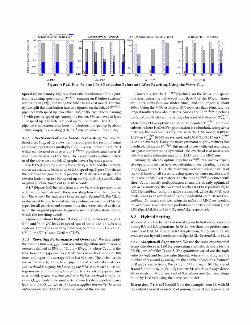
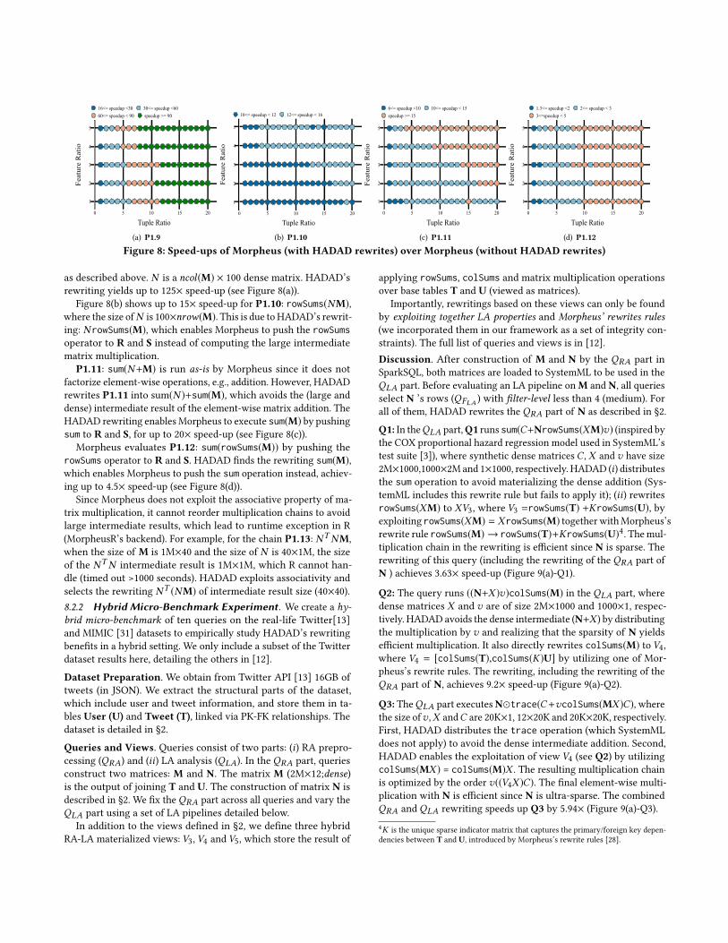
Figure 8: Speed-ups of Morpheus (with HADAD rewrites) over Morpheus (without HADAD rewrites)
as described above. N is a ncol(M) × 100 dense matrix. HADAD’s
rewriting yields up to 125× speed-up (see Figure 8(a)).
Figure 8(b) shows up to 15× speed-up for P1.10: rowSums(NM),
where the size ofN is 100×nrow(M). This is due toHADAD’s rewrit-
ing: NrowSums(M), which enables Morpheus to push the rowSumsoperator to R and S instead of computing the large intermediate
matrix multiplication.
P1.11: sum(N+M) is run as-is by Morpheus since it does not
factorize element-wise operations, e.g., addition. However, HADAD
rewrites P1.11 into sum(N )+sum(M), which avoids the (large and
dense) intermediate result of the element-wise matrix addition. The
HADAD rewriting enables Morpheus to execute sum(M) by pushing
sum to R and S, for up to 20× speed-up (see Figure 8(c)).
Morpheus evaluates P1.12: sum(rowSums(M)) by pushing the
rowSums operator to R and S. HADAD finds the rewriting sum(M),
which enables Morpheus to push the sum operation instead, achiev-
ing up to 4.5× speed-up (see Figure 8(d)).
Since Morpheus does not exploit the associative property of ma-
trix multiplication, it cannot reorder multiplication chains to avoid
large intermediate results, which lead to runtime exception in R
(MorpheusR’s backend). For example, for the chain P1.13: NTNM,
when the size of M is 1M×40 and the size of N is 40×1M, the size
of the NTN intermediate result is 1M×1M, which R cannot han-
dle (timed out >1000 seconds). HADAD exploits associativity and
selects the rewriting NT (NM) of intermediate result size (40×40).
8.2.2 Hybrid Micro-Benchmark Experiment. We create a hy-brid micro-benchmark of ten queries on the real-life Twitter[13]
and MIMIC [31] datasets to empirically study HADAD’s rewriting
benefits in a hybrid setting. We only include a subset of the Twitter
dataset results here, detailing the others in [12].
Dataset Preparation. We obtain from Twitter API [13] 16GB of
tweets (in JSON). We extract the structural parts of the dataset,
which include user and tweet information, and store them in ta-
bles User (U) and Tweet (T), linked via PK-FK relationships. The
dataset is detailed in §2.
Queries and Views. Queries consist of two parts: (i) RA prepro-
cessing (QRA) and (ii) LA analysis (QLA). In the QRA part, queries
construct two matrices: M and N. The matrix M (2M×12;dense)is the output of joining T and U. The construction of matrix N is
described in §2. We fix theQRA part across all queries and vary the
QLA part using a set of LA pipelines detailed below.
In addition to the views defined in §2, we define three hybrid
RA-LA materialized views: V3, V4 and V5, which store the result of
applying rowSums, colSums and matrix multiplication operations
over base tables T and U (viewed as matrices).
Importantly, rewritings based on these views can only be found
by exploiting together LA properties and Morpheus’ rewrites rules(we incorporated them in our framework as a set of integrity con-
straints). The full list of queries and views is in [12].
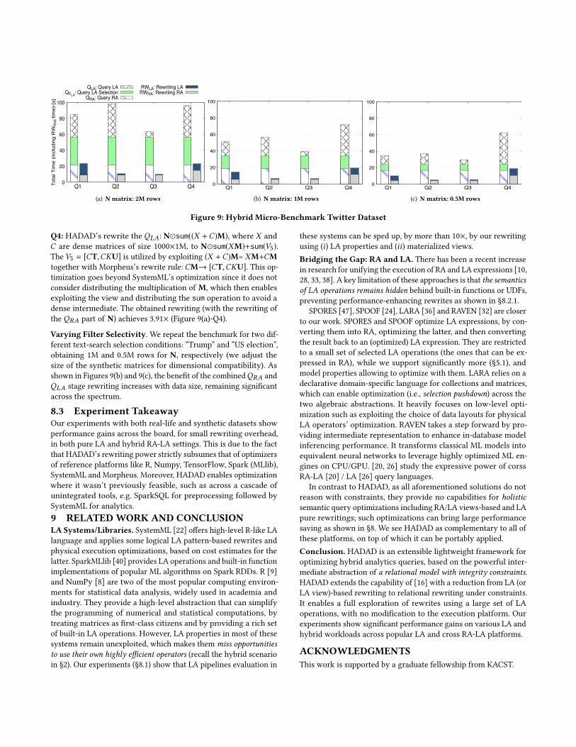
Discussion. After construction of M and N by the QRA part in
SparkSQL, both matrices are loaded to SystemML to be used in the
QLA part. Before evaluating an LA pipeline onM and N, all queries
select N ’s rows (QFLA ) with filter-level less than 4 (medium). For
all of them, HADAD rewrites the QRA part of N as described in §2.
Q1: In theQLA part,Q1 runs sum(C+NrowSums(XM)v) (inspired bythe COX proportional hazard regression model used in SystemML’s
test suite [3]), where synthetic dense matricesC , X and v have size
2M×1000,1000×2M and 1×1000, respectively. HADAD (i) distributesthe sum operation to avoid materializing the dense addition (Sys-
temML includes this rewrite rule but fails to apply it); (ii) rewritesrowSums(XM) to XV3, where V3 =rowSums(T) +KrowSums(U), byexploiting rowSums(XM) = XrowSums(M) togetherwithMorpheus’s
rewrite rule rowSums(M) → rowSums(T)+KrowSums(U)4. Themul-
tiplication chain in the rewriting is efficient since N is sparse. The
rewriting of this query (including the rewriting of the QRA part of
N ) achieves 3.63× speed-up (Figure 9(a)-Q1).
Q2: The query runs ((N+X )v)colSums(M) in the QLA part, where
dense matrices X and v are of size 2M×1000 and 1000×1, respec-
tively. HADAD avoids the dense intermediate (N+X ) by distributing
the multiplication by v and realizing that the sparsity of N yields
efficient multiplication. It also directly rewrites colSums(M) to V4,where V4 = [colSums(T),colSums(K)U] by utilizing one of Mor-
pheus’s rewrite rules. The rewriting, including the rewriting of the
QRA part of N, achieves 9.2× speed-up (Figure 9(a)-Q2).
Q3: TheQLA part executesN⊙trace(C+vcolSums(MX )C), wherethe size ofv ,X andC are 20K×1, 12×20K and 20K×20K, respectively.
First, HADAD distributes the trace operation (which SystemML
does not apply) to avoid the dense intermediate addition. Second,
HADAD enables the exploitation of view V4 (see Q2) by utilizing
colSums(MX ) = colSums(M)X . The resulting multiplication chain
is optimized by the order v((V4X )C). The final element-wise multi-
plication with N is efficient since N is ultra-sparse. The combined
QRA and QLA rewriting speeds up Q3 by 5.94× (Figure 9(a)-Q3).
4K is the unique sparse indicator matrix that captures the primary/foreign key depen-
dencies between T and U, introduced by Morpheus’s rewrite rules [28].
0
20
40
60
80
100
Q1 Q2 Q3 Q4TotalTime(includingRWfndtim
e)-[s]
QLA: Query LAQFLA: Query LA SelectionQRA: Query RA
RWLA: Rewriting LARWRA: Rewriting RA
(a) N matrix: 2M rows
0
20
40
60
80
100
Q1 Q2 Q3 Q4
(b) N matrix: 1M rows
0
20
40
60
80
100
Q1 Q2 Q3 Q4
(c) N matrix: 0.5M rows
Figure 9: Hybrid Micro-Benchmark Twitter Dataset
Q4: HADAD’s rewrite the QLA: N⊙sum((X +C)M), where X and
C are dense matrices of size 1000×1M, to N⊙sum(XM)+sum(V5).The V5 = [CT,CKU] is utilized by exploiting (X +C)M= XM+CMtogether with Morpheus’s rewrite rule: CM→ [CT,CKU]. This op-timization goes beyond SystemML’s optimization since it does not
consider distributing the multiplication of M, which then enables
exploiting the view and distributing the sum operation to avoid a
dense intermediate. The obtained rewriting (with the rewriting of
the QRA part of N) achieves 3.91× (Figure 9(a)-Q4).
Varying Filter Selectivity. We repeat the benchmark for two dif-
ferent text-search selection conditions: “Trump” and “US election”,
obtaining 1M and 0.5M rows for N, respectively (we adjust the
size of the synthetic matrices for dimensional compatibility). As
shown in Figures 9(b) and 9(c), the benefit of the combinedQRA and
QLA stage rewriting increases with data size, remaining significant
across the spectrum.
8.3 Experiment TakeawayOur experiments with both real-life and synthetic datasets show
performance gains across the board, for small rewriting overhead,
in both pure LA and hybrid RA-LA settings. This is due to the fact
that HADAD’s rewriting power strictly subsumes that of optimizers
of reference platforms like R, Numpy, TensorFlow, Spark (MLlib),
SystemML and Morpheus. Moreover, HADAD enables optimization
where it wasn’t previously feasible, such as across a cascade of
unintegrated tools, e.g. SparkSQL for preprocessing followed by
SystemML for analytics.
9 RELATEDWORK AND CONCLUSIONLA Systems/Libraries. SystemML [22] offers high-level R-like LA
language and applies some logical LA pattern-based rewrites and
physical execution optimizations, based on cost estimates for the
latter. SparkMLlib [40] provides LA operations and built-in function
implementations of popular ML algorithms on Spark RDDs. R [9]
and NumPy [8] are two of the most popular computing environ-
ments for statistical data analysis, widely used in academia and
industry. They provide a high-level abstraction that can simplify
the programming of numerical and statistical computations, by
treating matrices as first-class citizens and by providing a rich set
of built-in LA operations. However, LA properties in most of these
systems remain unexploited, which makes them miss opportunitiesto use their own highly efficient operators (recall the hybrid scenario
in §2). Our experiments (§8.1) show that LA pipelines evaluation in
these systems can be sped up, by more than 10×, by our rewriting
using (i) LA properties and (ii) materialized views.
Bridging the Gap: RA and LA. There has been a recent increase
in research for unifying the execution of RA and LA expressions [10,
28, 33, 38]. A key limitation of these approaches is that the semanticsof LA operations remains hidden behind built-in functions or UDFs,
preventing performance-enhancing rewrites as shown in §8.2.1.
SPORES [47], SPOOF [24], LARA [36] and RAVEN [32] are closer
to our work. SPORES and SPOOF optimize LA expressions, by con-
verting them into RA, optimizing the latter, and then converting
the result back to an (optimized) LA expression. They are restricted
to a small set of selected LA operations (the ones that can be ex-
pressed in RA), while we support significantly more (§5.1), and
model properties allowing to optimize with them. LARA relies on a
declarative domain-specific language for collections and matrices,
which can enable optimization (i.e., selection pushdown) across thetwo algebraic abstractions. It heavily focuses on low-level opti-
mization such as exploiting the choice of data layouts for physical
LA operators’ optimization. RAVEN takes a step forward by pro-
viding intermediate representation to enhance in-database model
inferencing performance. It transforms classical ML models into
equivalent neural networks to leverage highly optimized ML en-
gines on CPU/GPU. [20, 26] study the expressive power of corss
RA-LA [20] / LA [26] query languages.
In contrast to HADAD, as all aforementioned solutions do not
reason with constraints, they provide no capabilities for holisticsemantic query optimizations including RA/LA views-based and LA
pure rewritings; such optimizations can bring large performance
saving as shown in §8. We see HADAD as complementary to all of
these platforms, on top of which it can be portably applied.
Conclusion. HADAD is an extensible lightweight framework for
optimizing hybrid analytics queries, based on the powerful inter-
mediate abstraction of a relational model with integrity constraints.HADAD extends the capability of [16] with a reduction from LA (or
LA view)-based rewriting to relational rewriting under constraints.
It enables a full exploration of rewrites using a large set of LA
operations, with no modification to the execution platform. Our
experiments show significant performance gains on various LA and
hybrid workloads across popular LA and cross RA-LA platforms.
ACKNOWLEDGMENTSThis work is supported by a graduate fellowship from KACST.
REFERENCES[1] Amazon Review Data. https://nijianmo.github.io/amazon/index.html, Accessed
August, 2020.
[2] Breeze Wiki. https://github.com/scalanlp/breeze/wiki, Accessed June, 2020.
[3] Cox Proportional-Hazards Model. https://github.com/apache/systemds/blob/
master/scripts/algorithms/Cox-predict.dml, Accessed Feb, 2021.
[4] Kaggle Survey. https://www.kaggle.com/kaggle-survey-2019, Accessed June,
2020.
[5] Morpheus. https://github.com/lchen001/Morpheus, Accessed December, 2020.
[6] Native Blas in SystemDS. https://apache.github.io/systemds/native-backend,
Accessed June, 2020.
[7] Netflix Movie Rating. https://www.kaggle.com/netflix-inc/netflix-prize-data,
Accessed August, 2020.
[8] NumPy. https://numpy.org/, Accessed June, 2020.
[9] Project R. https://www.r-project.org/other-docs.html, Accessed June, 2020.
[10] Python/NumPy in Monetdb. https://tinyurl.com/11ljy21v, Accessed June, 2020.
[11] SparkMLlib. https://spark.apache.org/mllib, Accessed June, 2020.
[12] Technical Report. https://arxiv.org/abs/2103.12317.
[13] Twitter API. https://developer.twitter.com/en/docs, Accessed January, 2021.
[14] M. Abadi, P. Barham, J. Chen, Z. Chen, A. Davis, J. Dean, M. Devin, S. Ghemawat,
G. Irving, M. Isard, et al. Tensorflow: A System for Large-Scale Machine Learning.
In USENIX, pages 265–283, 2016.[15] S. Abiteboul, R. Hull, and V. Vianu. Foundations of Databases. Addison-Wesley,
1995.
[16] R. Alotaibi, D. Bursztyn, A. Deutsch, I. Manolescu, and S. Zampetakis. Towards
Scalable Hybrid Stores: Constraint-based Rewriting to the Rescue. In SIGMOD,pages 1660–1677, 2019.
[17] R. Alotaibi, B. Cautis, A. Deutsch, M. Latrache, I. Manolescu, and Y. Yang. ESTO-
CADA: Towards Scalable Polystore Systems. PVLDB, pages 2949–2952, 2020.[18] M. Armbrust, R. S. Xin, C. Lian, Y. Huai, D. Liu, J. K. Bradley, X. Meng, T. Kaftan,
M. J. Franklin, A. Ghodsi, et al. SparkSQl: Relational Data Processing in Spark.
In SIGMOD, pages 1383–1394, 2015.[19] S. Axler. Linear Algebra Done Right. Springer, 2015.[20] P. Barceló, N. Higuera, J. Pérez, and B. Subercaseaux. On the Expressiveness of
LARA: A Unified Language for Linear and Relational Algebra. In ICDT, pages6:1–6:20, 2020.
[21] D. Baylor, E. Breck, H.-T. Cheng, N. Fiedel, C. Y. Foo, Z. Haque, S. Haykal, M. Ispir,
V. Jain, L. Koc, et al. Tfx: A Tnsorflow-based Production-Scale Machine Learning
Platform. In SIGKDD, pages 1387–1395, 2017.[22] M. Boehm, M. W. Dusenberry, D. Eriksson, A. V. Evfimievski, F. M. Manshadi,
N. Pansare, B. Reinwald, F. R. Reiss, P. Sen, A. C. Surve, et al. SystemML: Declar-
ative Machine Learning on Spark. PVLDB, pages 1425–1436, 2016.[23] M. Boehm, A. V. Evfimievski, N. Pansare, and B. Reinwald. Declarative Machine
Learning Classification of Basic Properties and Types. arXiv:1605.05826, 2016.[24] M. Boehm, B. Reinwald, D. Hutchison, P. Sen, A. V. Evfimievski, and N. Pansare.
On Optimizing Operator Fusion Plans for Large-Scale Machine Learning in
SystemML. PVLDB, pages 1755–1768, 2018.[25] J.-H. Böse, V. Flunkert, J. Gasthaus, T. Januschowski, D. Lange, D. Salinas, S. Schel-
ter, M. Seeger, and Y. Wang. Probabilistic Demand Forecasting at Scale. PVLDB,pages 1694–1705, 2017.
[26] R. Brijder, F. Geerts, J. V. den Bussche, and T. Weerwag. On the Expressive Power
of Query Languages for Matrices. ACM Trans. Database Syst., pages 15:1–15:31,
2019.
[27] A. K. Chandra and P. M. Merlin. Optimal Implementation of Conjunctive Queries
in Relational Databases. In ACM symposium on Theory of computing, pages 77–90,1977.
[28] L. Chen, A. Kumar, J. Naughton, and J. M. Patel. Towards Linear Algebra Over
Normalized Data. PVLDB, pages 1214–1225, 2017.[29] I. Ileana. Query Rewriting Using Views : a Theoretical and Practical Perspective.
Theses, Télécom ParisTech, Oct. 2014.
[30] I. Ileana, B. Cautis, A. Deutsch, and Y. Katsis. Complete Yet Practical Search for
Minimal Query Reformulations Under Constraints. In SIGMOD, pages 1015–1026,2014.
[31] A. Johnson et al. MIMIC-III. http://www.nature.com/articles/ sdata201635, 2016.[32] K. Karanasos, M. Interlandi, D. Xin, F. Psallidas, R. Sen, K. Park, I. Popivanov,
S. Nakandal, S. Krishnan,M.Weimer, et al. Extending Relational Query Processing
with ML Inference. In CIDR, 2020.[33] D. Kernert, F. Köhler, and W. Lehner. Bringing Linear Algebra Objects to Life in
a Column-Criented in-Memory Database. In In Memory Data Management andAnalysis, pages 44–55. Springer, 2013.
[34] A. Kumar, M. Boehm, and J. Yang. Data Management in Machine Learning:
Challenges, Techniques, and Systems. In SIGMOD, pages 1717–1722, 2017.[35] A. Kumar, R. McCann, J. Naughton, and J. M. Patel. Model Selection Management
Systems: The Next Frontier of Advanced Analytics. In SIGMOD, pages 17–22,2016.
[36] A. Kunft, A. Katsifodimos, S. Schelter, S. Breß, T. Rabl, and V. Markl. An Interme-
diate Representation for Optimizing Machine Learning Pipelines. PVLDB, pages1553–1567, 2019.
[37] K. Kuttler. Linear Algebra: Theory and Applications. The Saylor Foundation, 2012.[38] S. Luo, Z. J. Gao, M. Gubanov, L. L. Perez, and C. Jermaine. Scalable Linear
Algebra on a Relational Database System. In ICDE, pages 1224–1238, 2018.[39] J. MacQueen et al. Some methods for classification and analysis of multivariate
observations. In Proceedings of the fifth Berkeley symposium on mathematicalstatistics and probability, pages 281–297, 1967.
[40] X. Meng, J. Bradley, B. Yavuz, E. Sparks, S. Venkataraman, D. Liu, J. Freeman,
D. Tsai, M. Amde, S. Owen, et al. MLlib: Machine Learning in Apache Spark. TheJournal of Machine Learning Research, pages 1235–1241, 2016.
[41] M. Milani, S. Hosseinpour, and H. Pehlivan. Rule-based Production of Mathemat-
ical Expressions. Mathematics, 6:254, 11 2018.[42] T. M. Mitchell. Machine Learning. McGraw-Hill, 1997.
[43] D. Sculley, G. Holt, D. Golovin, E. Davydov, T. Phillips, D. Ebner, V. Chaudhary,
M. Young, J.-F. Crespo, and D. Dennison. Hidden Technical Debt in Machine
Learning Systems. In NeurIPS, pages 2503–2511, 2015.[44] J. Sommer, M. Boehm, A. V. Evfimievski, B. Reinwald, and P. J. Haas. MNC:
Structure-Exploiting Sparsity Estimation for Matrix Expressions. In SIGMOD,pages 1607–1623, 2019.
[45] E. R. Sparks, A. Talwalkar, D. Haas, M. J. Franklin, M. I. Jordan, and T. Kraska.
Automating Model Search for Large Scale Machine Learning. In ACM Symposiumon Cloud Computing, pages 368–380, 2015.
[46] A. Thomas and A. Kumar. A Comparative Evaluation of Systems for Scalable
Linear Algebra-based Analytics. PVLDB, pages 2168–2182, 2018.[47] Y. R. Wang, S. Hutchison, J. Leang, B. Howe, and D. Suciu. SPORES: Sum-Product
Optimization via Relational Equality Saturation for Large Scale Linear Algebra.
PVLDB, pages 1919–1932, 2020.