Rochester Institute of TechnologyRIT Scholar Works

Presentations and other scholarship Faculty & Staff Scholarship

3-15-2006

H-Infinity Controller Design for StructuralDampingDarren RowenThe Aerospace Corp.

Mark A. HopkinsRochester Institute of Technology

Follow this and additional works at: https://scholarworks.rit.edu/other

This Conference Paper is brought to you for free and open access by the Faculty & Staff Scholarship at RIT Scholar Works. It has been accepted forinclusion in Presentations and other scholarship by an authorized administrator of RIT Scholar Works. For more information, please contactritscholarworks@rit.edu.

Recommended CitationDarren W. Rowen, Mark A. Hopkins, "H-infinity controller design for structural damping", Proc. SPIE 6169, Smart Structures andMaterials 2006: Damping and Isolation, 616904 (15 March 2006); doi: 10.1117/12.658327; https://doi.org/10.1117/12.658327

Copyright 2006 Society of Photo-Optical Instrumentation Engineers. This paper was published by SPIE and is made available as an electronic reprint (preprint) with permission of SPIE. One print or electronic copy may be made for personal use only. Systematic or multiple reproduction, distribution to multiple locations via electronic or other means, duplication of any material in this paper for a fee or for commercial purposes, or modification of the content of the paper are prohibited. 

*darren.w.rowen@aero.org; phone 1 310 336-3107; fax 1 310 336-6548 **mark.hopkins@rit.edu; phone 1 585 475-6640; fax 1 585 475-5845

H-Infinity controller design for structural damping

Darren W. Rowen*ab, Mark A. Hopkins**b aThe Aerospace Corporation, 2350 East El Segundo Blvd., El Segundo, CA, USA 90245; bRochester Institute of Technology, 79 Lomb Memorial Dr., Rochester, NY, USA 14623

ABSTRACT This paper describes a multivariable controller design procedure that uses mixed-sensitivity H-infinity control theory. The design procedure is based on the assumption that structural noise can be modeled as entering a state-space system through a random input matrix. The design process starts with a full-order flexible state-space model that undergoes a frequency-weighted balanced truncation to obtain a reduced-order model with excellent low frequency matching. Weighting functions are then created to specify the desired frequency range for disturbance rejection and controller bandwidth. A structural noise input matrix is also designed to identify system modes where maximal damping is desired. An augmented plant is then assembled using the reduced-order model, weighting functions and structural noise input matrix to create a mixed-sensitivity configuration. A state-space controller is then realized using an H-infinity design algorithm. A two-input, three-output, doubly cantilevered beam system provides a design example. A 174th-order, discrete-time, state-space model of the cantilevered beam system was used to generate a reduced 40th-order model. A 55th-order H-infinity controller was then designed with a controller bandwidth of approximately 300 Hz. This non-square modern controller uses feedback signals from two piezoelectric sensors, each collocated with one of two piezoelectric actuators, and one highly non-collocated accelerometer. The two piezoelectric actuators provide the control actuation. Frequency analysis and time-domain simulations are utilized to demonstrate the damping performance. Keywords: MIMO, H-infinity, control, controller design, flexible, mixed-sensitivity

1. INTRODUCTION A 174th order, discrete-time, state-space model of a doubly cantilevered beam and its frequency response data was derived from input-output measurements. The system has 2 inputs and 3 outputs, with one of the outputs being highly non-collocated. The system configuration is shown in Figure 1. The first five significant bending modes of the system are located at 16 Hz, 37 Hz, 101 Hz, 193 Hz, and 284 Hz. The system exhibits very large amplitude oscillations when excited at these frequencies. The design objective is to create a controller that will dampen beam oscillations for these bending modes along with any other system modes in the low-frequency band (3 Hz – 300 Hz). The methods used in this design process can be applied to flexible body control for both space and ground based systems. The model reduction objective is to obtain a 40th order model that best approximates the 174th order model in the low-frequency band. The reduced model is anticipated to sacrifice high frequency model accuracy for the attainment of a smaller system model. Ultimately, this reduced model will be used to obtain a reduced-order controller.

2. FREQUENCY WEIGHTED MODEL ORDER REDUCTION A third-party frequency weighted balanced truncation (FWBT) algorithm is used to generate a reduced order model. The SLICOT ‘fwbred’1 MATLAB function uses the SLICOT AB09ID1 library. To obtain the desired 40th order reduced model, a frequency weighting function is created to emphasize frequency regions where close matching is most important. The singular values of the frequency weighting function are plotted in Figure 2 along with the minimum and maximum singular values of the original and reduced models.

Smart Structures and Materials 2006: Damping and Isolation, edited by William W. Clark, Mehdi Ahmadian,Arnold Lumsdaine, Proc. of SPIE Vol. 6169, 616904, (2006) · 0277-786X/06/$15 · doi: 10.1117/12.658327

Proc. of SPIE Vol. 6169 616904-1

bI6O6I6CLIC 26UOLOnbn 9uq

bIGOGIGCL!C VC19OL2

GLubn2 9uq

VCCGIGLOW(

Onbn

20

cuJ

CA

E

M'qnjbL!W9Ll G9LJJ 2

1WecouqsL1 BSS 2p!LJJ 2OCf Miqf4J CLJJ

Full Order Model—

________ 40th Order Model [FWBT]

Weighting Fn

40

30

20-

10—

Singular Values

l0 •0 101

Frequency (Hz)

10 l0

-10

-20

Figure 1: Doubly Cantilevered Beam System Figure 2 is very useful to get an overall picture of how well the reduced model’s matching is, as singular values reflect all input-output paths of this multiple-input-multiple-output (MIMO) system. In the range below 2 kHz, it is difficult to distinguish one model from another. The plots are practically identical. It is in the region above 2 kHz that a divergence can be noticed. Although high-frequency divergence is clearly visible, it is also clear that the reduced model shoots a rough average of the response in this region. This is a desirable approximation when compared to other possible high-frequency approximations, like simple roll-off or a 0-dB gain.

Figure 2: Maximum and Minimum Singular Values for the 174th order model and the reduced 40th order model

Proc. of SPIE Vol. 6169 616904-2

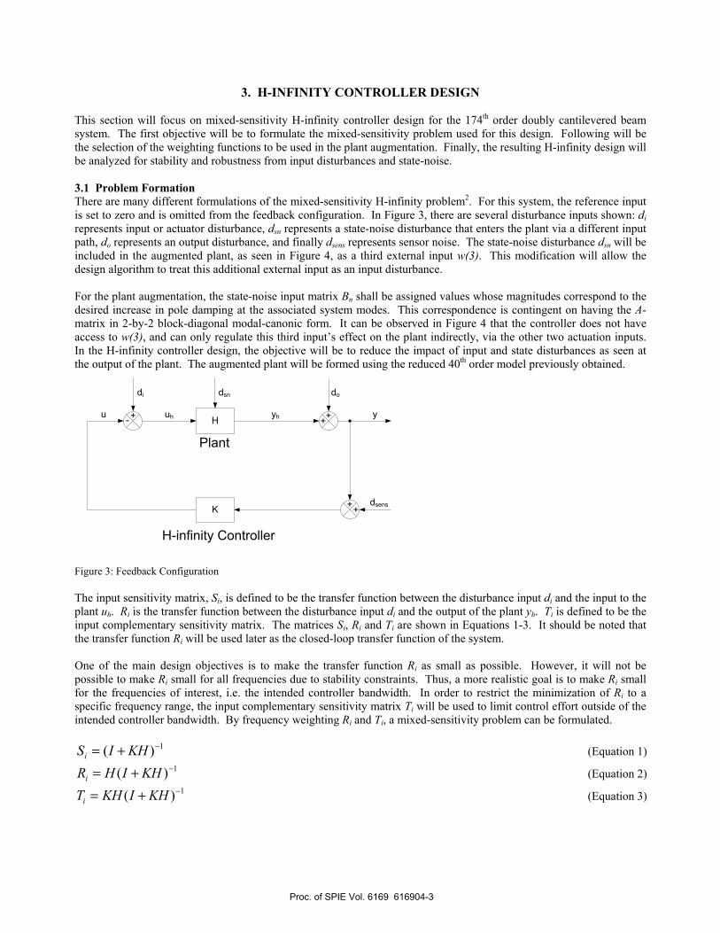
3. H-INFINITY CONTROLLER DESIGN This section will focus on mixed-sensitivity H-infinity controller design for the 174th order doubly cantilevered beam system. The first objective will be to formulate the mixed-sensitivity problem used for this design. Following will be the selection of the weighting functions to be used in the plant augmentation. Finally, the resulting H-infinity design will be analyzed for stability and robustness from input disturbances and state-noise. 3.1 Problem Formation There are many different formulations of the mixed-sensitivity H-infinity problem2. For this system, the reference input is set to zero and is omitted from the feedback configuration. In Figure 3, there are several disturbance inputs shown: di represents input or actuator disturbance, dsn represents a state-noise disturbance that enters the plant via a different input path, do represents an output disturbance, and finally dsens represents sensor noise. The state-noise disturbance dsn will be included in the augmented plant, as seen in Figure 4, as a third external input w(3). This modification will allow the design algorithm to treat this additional external input as an input disturbance. For the plant augmentation, the state-noise input matrix Bn shall be assigned values whose magnitudes correspond to the desired increase in pole damping at the associated system modes. This correspondence is contingent on having the A-matrix in 2-by-2 block-diagonal modal-canonic form. It can be observed in Figure 4 that the controller does not have access to w(3), and can only regulate this third input’s effect on the plant indirectly, via the other two actuation inputs. In the H-infinity controller design, the objective will be to reduce the impact of input and state disturbances as seen at the output of the plant. The augmented plant will be formed using the reduced 40th order model previously obtained.

- H

K

H-infinity Controller

+u

Plant

++

++

uh yh y

dsens

dodi dsn

Figure 3: Feedback Configuration The input sensitivity matrix, Si, is defined to be the transfer function between the disturbance input di and the input to the plant uh. Ri is the transfer function between the disturbance input di and the output of the plant yh. Ti is defined to be the input complementary sensitivity matrix. The matrices Si, Ri and Ti are shown in Equations 1-3. It should be noted that the transfer function Ri will be used later as the closed-loop transfer function of the system. One of the main design objectives is to make the transfer function Ri as small as possible. However, it will not be possible to make Ri small for all frequencies due to stability constraints. Thus, a more realistic goal is to make Ri small for the frequencies of interest, i.e. the intended controller bandwidth. In order to restrict the minimization of Ri to a specific frequency range, the input complementary sensitivity matrix Ti will be used to limit control effort outside of the intended controller bandwidth. By frequency weighting Ri and Ti, a mixed-sensitivity problem can be formulated.

1)( −+= KHISi (Equation 1) 1)( −+= KHIHRi (Equation 2)

1)( −+= KHIKHTi (Equation 3)

Proc. of SPIE Vol. 6169 616904-3

Three weighting matrices are applied to the aforementioned functions to form the following cost function:

⎥⎥⎥

⎦

⎤

⎢⎢⎢

⎣

⎡=

i

i

i

zw

TWRWSW

T

3

2

1

(Equation 4)

The mixed-sensitivity H-infinity problem can then be formulated using cost function Tzw: Minimize:

∞zwT

w(1:3)Br+

y(1:3)

z-1

Bn

Cr

Ar

Dr

W1

W2

W3

K

z(6:7)

z(3:5)

z(1:2)

H-infinity Controller

Augmented Plant P

+++- ++

u(1:2)

w(3) [dsn]

w(1:2) [di]

Figure 4: Mixed-sensitivity augmented plant configuration. The 40th order reduced model is represented by the matrices Ar, Br, Cr and Dr. 3.2 Design Procedure In order to build the augmented plant, the matrix Bn had to be selected in addition to the weighting matrices. In the final closed-loop system configuration, state-noise can be thought of as entering the system through an unknown matrix Bn. However, for the purpose of the H-infinity controller design, the elements of the Bn matrix were assigned according to a bandpass filter as shown in Figure 6. Larger magnitude values in Bn will correspond to system modes at which maximum closed-loop pole damping is desired. Furthermore, the sign of each element in Bn was hand-selected to meet several objectives. Because the matrix Bn will be ultimately appended to the reduced order Br matrix, the value and respective sign of each element in Bn will contribute to changes in the compensated open-loop transmission zeros. This is not necessarily a problem, as long as none of the transmission zeros are moved very close to the unit circle from a former position that was initially much closer to the origin. The reason for this requirement is that the H-infinity control algorithm will seek to compensate these artificial transmission zeros by placing controller poles in the same vicinity. But in the real system, state-noise does not actually enter through the Bn used in the design process. Thus any controller poles placed near the unit circle for compensation would produce an undesirable magnitude increase in the closed-loop frequency response, due to the fact that there aren’t really transmission zeros in those locations.

Proc. of SPIE Vol. 6169 616904-4

-20 — _______________________________________________________

Plant

Appended Reduced Order Model

30 -

I

io to1Frequency (HZ)

Viluu of ths mitrI utid I thiH_ controllsr duign

'C 'C ,OC'C*'C,C'C 'C

_50 'C

'C 'C

'C

'C ..-250 . . . ... . . ...-300 I ...I !,!!!!i!I 1 I

io4 1o 10' 10_I 10' 10' 10' 10' ioCorresponding Modal Freqoency lHzl

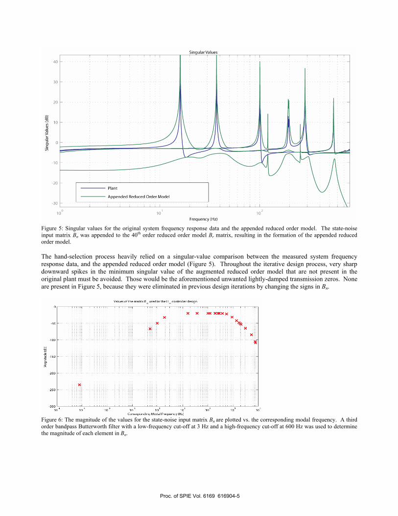
Figure 5: Singular values for the original system frequency response data and the appended reduced order model. The state-noise input matrix Bn was appended to the 40th order reduced order model Br matrix, resulting in the formation of the appended reduced order model. The hand-selection process heavily relied on a singular-value comparison between the measured system frequency response data, and the appended reduced order model (Figure 5). Throughout the iterative design process, very sharp downward spikes in the minimum singular value of the augmented reduced order model that are not present in the original plant must be avoided. Those would be the aforementioned unwanted lightly-damped transmission zeros. None are present in Figure 5, because they were eliminated in previous design iterations by changing the signs in Bn.

Figure 6: The magnitude of the values for the state-noise input matrix Bn are plotted vs. the corresponding modal frequency. A third order bandpass Butterworth filter with a low-frequency cut-off at 3 Hz and a high-frequency cut-off at 600 Hz was used to determine the magnitude of each element in Bn.

Proc. of SPIE Vol. 6169 616904-5

It is important to understand that the controller does not have access to the system via the state-noise input. Therefore, the only way for the controller to minimize the MIMO transfer function from the input at Bn to each of the respective system outputs is to increase the closed-loop pole damping, which is the main control design objective. The selection of weighting functions (unrelated to the selection of Bn) to be used in the plant augmentation was largely a trial and error process. The starting point was to try a 0 dB allpass filter for W2, while assigning W1 and W3 to zero. The resulting controller was combined with the full-order model to form an unstable closed-loop system.. Note that the design approach uses a reduced-order model in the appended plant configuration. This means that the design algorithm will guarantee a stable closed-loop system when the controller is combined with the reduced-order model. However, the objective is to obtain a reduced-order controller that stabilizes the real system, which is best approximated by the full-order model. As seen in Figure 2, the reduced-order model does not capture the same high-frequency response as the full-order model. Thus a design that results in instability at high frequency was not surprising. The next step was to try implementing a highpass filter for the W3 weighting function to decrease the controller gain in the high frequency region. Unfortunately, instability still occurred at very low frequencies (less than 1 Hz). Thus, a bandstop filter was tried for the weighting function W3. This resolved stability issues in the lower frequency range, but the high frequency region was still not entirely stabilized. By choosing a lowpass filter for the W2 weighting function, a much smaller controller gain was obtained in the high-frequency band. Adjustments to the weighting function gains, filter orders, and cut-off frequencies led to the final design. In the final design, Butterworth filters for the weighting functions were created with the parameters described in Table 1. W1 can be used to weight the “tracking” performance of a control system. Because the control objective is simply to reduce the output magnitude, the W1 weighting function is not required for this control problem and is set to zero. Gain Cut-off Frequency(s) [Hz] Filter Order Filter Type W1 0 N/A 0 N/A W2 -20 dB 350 1 Lowpass W3 40 dB [ 0.2 , 4000 ] 3 Bandstop

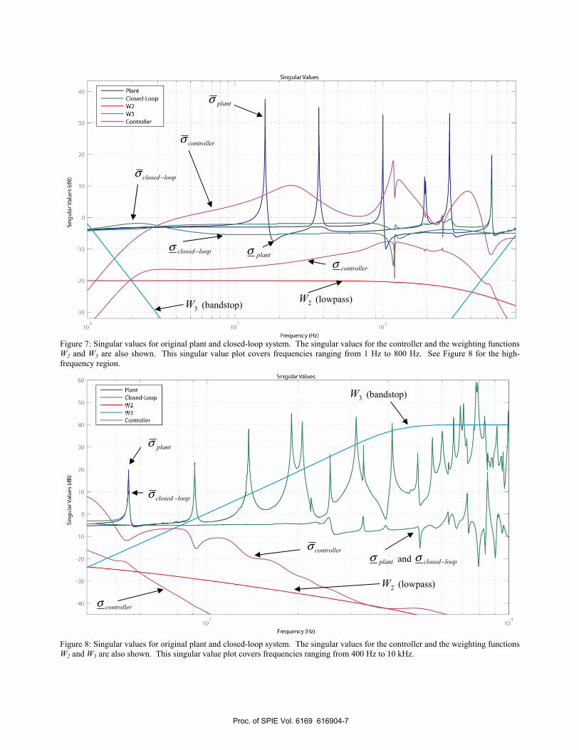
Table 1: Weighting Function Parameters In Figure 7 and Figure 8, the singular values of the weighting functions are plotted along with the first and last singular values of the open and closed-loop systems. The singular values of the stand-alone controller are also shown for reference. Between them, these two figures cover the range of frequencies from 1-Hz to 10kHz. 3.3 Synthesis and Analysis For H-infinity design synthesis, the SLICOT based MATLAB function ‘dishin’3 which uses the SLICOT SB10DD3 library was used to generate the state-space representation of the controller K. The resulting design is a 55th order controller. This controller size is notably larger than the 40th order reduced system model, yet less than 1/3rd of the full 174th order model. When the 174th-order system model is used, the closed loop model is 229th order. The resulting closed-loop system frequency response is displayed in two singular value plots: Figure 7 and Figure 8. After observing Figure 7, it can be seen that closed-loop singular values are, in general, much smaller in magnitude than the plotted singular values of the original plant. In particular, the first five major modes peak at over 30 dB in the original plant, while the closed-loop system manages to contain these peaks to less than 0 dB. In the controller roll-off region, between 300-Hz and 1-kHz there is little to no increase in the system response, an indication of very little controller spillover. In the frequency band beyond 1 kHz, the closed-loop singular values match the open-loop values very closely. It is only in the sharp peaks that any difference can be observed. Ideally, all of the peak values in this frequency range would be no greater than the original plant peak values. Upon closer inspection, it can be seen that this is largely the case. In most cases, the closed-loop singular values are actually less than the original plant values. There are a few instances where a very slight increase can be observed over the original plant values. Overall, the high-frequency response is almost exactly the same as the open-loop response. That indicates very good high-frequency controller characteristics.

Proc. of SPIE Vol. 6169 616904-6

Frequency (Hz)

40 — Plant

Closed-LoopW2W3

30 — Controller

20 —

to.0

ci 0—

Singular Values

ID 10

Singular Values

Plant

Closed-LoopW2W3

Controller40•

30 —

20 —

to —

-30

40

10Frequency (Hz)

Figure 7: Singular values for original plant and closed-loop system. The singular values for the controller and the weighting functions W2 and W3 are also shown. This singular value plot covers frequencies ranging from 1 Hz to 800 Hz. See Figure 8 for the high-frequency region.

Figure 8: Singular values for original plant and closed-loop system. The singular values for the controller and the weighting functions W2 and W3 are also shown. This singular value plot covers frequencies ranging from 400 Hz to 10 kHz.

plantσ

plantσ loopclosed −σ

loopclosed −σ

3W (bandstop) 2W (lowpass)

controllerσ

controllerσ

3W (bandstop)

plantσ loopclosed−σand

controllerσ

controllerσ

2W (lowpass)

loopclosed −σ

plantσ

Proc. of SPIE Vol. 6169 616904-7

Pole-Zero Map

.....

-_..I0:;....

..

.

.•

. .

I -.......

.......

I

...

.. I..:...

. ..

.

-. NH295H.

... ZN.

. . N

I I

X OLPlantPoles* OLcontrollerPoles -

0 Closed-LoopPoles0 Transmission Zeros

007 - 233H\a'

. ... .. .. .... ..to . . . .. .

006- 0 S184Hz

005 - 01 009 008 00/ 006 005 004 003 002 001

0 146Hz

0.04- .. .... .. ... ... .. ..

....... . .. .115Hz

0.03 —.. I . I I

0.99 0.991 0.992 0.993 0.994 0.995 0.996 0.997 0.998 0.999Real

x io Pole-Zero MapI •.• •. I I I I

)t OLPlantPoles

* OLControllerPoleso Closed-Loop Poleso Transmission Zeros

12 o35.6Hz

01 009 008 007 006 005 004 003 002 001

28.1Hz

..... ... .... .. •..o•. .

•

.... ...

.... ......

. H . 22.2Hz

C 116H

•139Hz

I I I I. I

0.999 0.9992 0.9994 0.9996 0.9998 1

Real

Figure 9: Pole-zero map showing transmission zeros as well as open and closed-loop poles. This figure concentrates on the region of lightly damped poles in the 100 Hz - 300 Hz region.

Figure 10: Pole-zero map showing Transmission zeros as well as open and closed-loop poles. This figure concentrates on the region of lightly damped poles in the 10 Hz – 100 Hz region.

Proc. of SPIE Vol. 6169 616904-8

Com

pens

ated

Ope

n Lo

op M

agni

tude

(dB

)

NJ

do

th

NJ

a 0

0 0

0 0

0 0

0 0

After reviewing Figure 7 and Figure 8, it is clear that a reduction in the closed-loop transfer function (Ri) is achieved in the desired control bandwidth (3 Hz – 300 Hz). This reduction shows an improvement in input disturbance rejection in this region of interest. In Figure 9 and Figure 10, compensated open-loop poles and transmission zeros are plotted along with the closed-loop poles. The areas enlarged in these figures cover poles of particular interest. Ideally, the compensated open-loop poles would all move toward more heavily damped positions in closed-loop. The compensated open-loop poles of particular interest are located at positions corresponding to a damping ratio of much less than 1%. As desired, many of the compensated open-loop poles were moved to significantly more heavily-damped locations.

Figure 11: Nichols plot of the characteristic loci Figure 11 shows the characteristic loci of the compensated open-loop system plotted on a Nichols chart. From this plot, estimates of the stability margins can be obtained. It can be estimated that the gain margin is approximately 9 dB, while the phase margin is approximately 40 degrees. Because the characteristic loci are MIMO plots, quantitative estimates of the stability margins are not as straightforward as they are in a SISO Nichols chart [4], but they are nevertheless good qualitative indicators of relative stability. 3.4 Performance Analysis In order to investigate the impact of state-noise on the system, the transfer function from w(3) to the outputs y(1:3) (see Figure 4) was determined using random Gaussian zero-mean values for the matrix Bn, which has 174 rows and only one column. For the purpose of evaluating state-noise reduction in the control bandwidth, only the values in Bn corresponding to modes covering the range 16 Hz – 550 Hz were assigned nonzero values. Outside of this range, the controller gain is very small; thus, the response from the closed loop system will, ideally, match the open-loop plant very closely. Ten independent trials were conducted with different random values assigned to Bn. For each trial, the random values in Bn were assigned a variance of 1/10. The results were then averaged to obtain the transfer functions plotted in Figure 13. The magnitudes from state-noise input w(3) to each output are shown for both the open-loop and closed-loop systems, based on the 174th order model. It is readily observed that many of the large peaks evident in the open-loop system have

16.03 Hz

17.72 Hz

284.79 Hz

549.56 Hz

Proc. of SPIE Vol. 6169 616904-9

25

0 0.1 0.2 0.3 0.4 0.5 0.6 0.7 0.8 0.9Drping Ratio

been greatly reduced in the closed-loop system. This design is successful in reducing sensitivity to state-noise on these particular modes. There is a direct correlation between the pole damping seen in Figure 9 and Figure 10 and the reduced state-noise sensitivity that is demonstrated in Figure 13.

Figure 12: Perturbed plant pole frequency variation is shown as a percentage, which is assigned as a function of corresponding pole damping ratio. Poles with greater damping are harder to determine in the system identification process, and thus are varied more than poles with very little damping. To demonstrate control robustness, the original plant was perturbed by varying the pole frequencies as a function of damping ratio. This pole variation necessitates having the A-matrix in 2-by-2 block-diagonal modal-canonic form. Using the frequency variation profile from Figure 12, two perturbed systems were generated: one with positive frequency variation, and a second with negative. Recall that the original plant was generated using a system identification process. Thus, poles that are very lightly damped will produce greater oscillations in the identification process and will be more accurately identified than more heavily damped poles which produce relatively small oscillations. It is conceivable that other sources could contribute to plant variation. Thermal deformations, to name one example, could contribute to pole movement in the actual system both for lightly and heavily damped poles. However, for this study, it was assumed that such contributors would be relatively small. By modifying the augmented plant formulation (Figure 4) accordingly, the design could be tailored to better cope with significant plant variations caused by other sources. Figure 13 and Figure 14 plot the closed-loop performance with pole frequency variation in addition to the nominal closed-loop performance. Time domain simulations were performed to further analyze the damping performance of the closed loop system. The state-noise input matrix, Bn, was once again assigned Gaussian random zero-mean values for elements corresponding to modal frequencies between 16 Hz and 550 Hz. The impulse response from the state-noise disturbance input dsn to output 3 was simulated, and the results are shown in Figure 14. Simulations were also preformed for outputs 1 and 2, however they are not shown. Output 3 (the accelerometer) is the best output for evaluating damping performance, as it is highly non-collocated with respect to the piezoelectric actuators and it is also located on a thin piece of shim stock (see Figure 1). At 0.07 seconds, the averaged mean-square response of the closed-loop system at the non-collocated sensor is almost 12 times smaller than that of the open-loop plant. This time domain simulation demonstrates the high performance and robustness of the controller design.

Proc. of SPIE Vol. 6169 616904-10

Magnitude at Outputs 1-3 from the State Noise Input on 16-550 Hz Modes:10' OL Plant

Frequency (Hz) CL Nominal

CL +Freq VariationL-FreqVariation

102

Frequency (Hz)40i102

Frequency (Hz)

-s Mean-Square Impulse Response Simulation from d to Output 3 (Averaged,1 00 runs)xlO Sn

8

7

a'6

aCa,(0

o4C(0a)

0.01 0.02 0.03 0.04Time (sec)

0.05 0.06 0.01

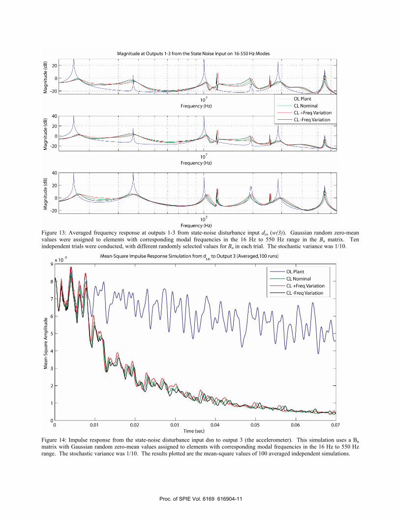
Figure 13: Averaged frequency response at outputs 1-3 from state-noise disturbance input dsn (w(3)). Gaussian random zero-mean values were assigned to elements with corresponding modal frequencies in the 16 Hz to 550 Hz range in the Bn matrix. Ten independent trials were conducted, with different randomly selected values for Bn in each trial. The stochastic variance was 1/10.

Figure 14: Impulse response from the state-noise disturbance input dsn to output 3 (the accelerometer). This simulation uses a Bn matrix with Gaussian random zero-mean values assigned to elements with corresponding modal frequencies in the 16 Hz to 550 Hz range. The stochastic variance was 1/10. The results plotted are the mean-square values of 100 averaged independent simulations.

Proc. of SPIE Vol. 6169 616904-11

* ftp://wgs.esat.kuleuven.ac.be/pub/WGS/REPORTS/SLWN2002-5.ps.Z ** ftp://wgs.esat.kuleuven.ac.be/pub/WGS/REPORTS/SLWN1999-12.ps.Z

4. CONCLUSION The H-infinity design obtained meets the design objective of dampening beam oscillations for system modes in the low-frequency band (3 Hz – 300 Hz) in addition to several system modes greater than 300 Hz. The time domain analysis demonstrates the overall dampening performance, while the frequency domain analysis shows the performance for individual system modes. By using a reduced order model, the 55th order H-infinity controller was obtained. This size is less than 1/3rd of the full 174th order system identified plant model. The design process demonstrates how to obtain a reduced-order controller that meets the design objective. The controller size can be scaled to meet the available hardware capability by modifying the model reduction process accordingly. The simulations and calculated closed-loop frequency response data are the best demonstration of how the real system would perform with the controller. It should be noted that controller design is often an iterative process, which includes testing with real hardware. The design presented is intended to be an initial point in the cycle, which could involve several iterations before a final controller design is selected.

REFERENCES 1.* A. Varga, “New Numerical Software for Model and Controller Reduction”, Working Group of Software, SLICOT, 2002. 2. K. Zhou and J. Doyle, Essentials of Robust Control, Chapter 6, Prentice Hall, Upper Saddle River, 1998. 3.** D. Gu, P. Petkov and M. Konstantinov, “H∞ and H2 Optimization Toolbox in SLICOT”, Working Group of Software, SLICOT, 1999. 4. J. Maciejowski, Multivariable Feedback Design, Addison Wesley, New York, 1989.

Proc. of SPIE Vol. 6169 616904-12