Comparison Theorems in Riemannian Geometry

J.-H. Eschenburg

0. Introduction

The subject of these lecture notes is comparison theory in Riemannian geometry:What can be said about a complete Riemannian manifold when (mainly lower) boundsfor the sectional or Ricci curvature are given? Starting from the comparison theory forthe Riccati ODE which describes the evolution of the principal curvatures of equidis-tant hypersurfaces, we discuss the global estimates for volume and length given byBishop-Gromov and Toponogov. An application is Gromov’s estimate of the numberof generators of the fundamental group and the Betti numbers when lower curvaturebounds are given. Using convexity arguments, we prove the ”soul theorem” of Cheegerand Gromoll and the sphere theorem of Berger and Klingenberg for nonnegative cur-vature. If lower Ricci curvature bounds are given we exploit subharmonicity insteadof convexity and show the rigidity theorems of Myers-Cheng and the splitting theoremof Cheeger and Gromoll. The Bishop-Gromov inequality shows polynomial growth offinitely generated subgroups of the fundamental group of a space with nonnegative Riccicurvature (Milnor). We also discuss briefly Bochner’s method.

The leading principle of the whole exposition is the use of convexity methods.Five ideas make these methods work: The comparison theory for the Riccati ODE,which probably goes back to L.Green [15] and which was used more systematically byGromov [20], the triangle inequality for the Riemannian distance, the method of supportfunction by Greene and Wu [16],[17],[34], the maximum principle of E.Hopf, generalizedby E.Calabi [23], [4], and the idea of critical points of the distance function which wasfirst used by Grove and Shiohama [21]. We have tried to present the ideas completelywithout being too technical.

These notes are based on a course which I gave at the University of Trento in March1994. It is a pleasure to thank Elisabetta Ossanna and Stefano Bonaccorsi who haveworked out and typed part of these lectures. We also thank Evi Samiou and RobertBock for many valuable corrections.

Augsburg, September 1994

J.-H. Eschenburg

1

1. Covariant derivative and curvature.

Notation: By M we always denote a smooth manifold of dimension n. For p ∈M ,the tangent space at p is denoted by TpM , and TM denotes the tangent bundle. IfM ′ is another manifold and f : M → M ′ a smooth (i.e. C∞) map, its differential atsome point p ∈ M is always denoted by dfp : TpM → Tf(p)M

′. For v ∈ TpM we writedfp(v) = dfp.v = ∂vf . If c : I → M is a (smooth) curve, we denote its tangent vectorby c′(t) = dc(t)/dt = dct.1 ∈ Tc(t)M (where 1 ∈ TtI = IR). If f : M → IR, thendfp ∈ (TpM)∗. If M is a Riemannian manifold, i.e. there exists a scalar product < , >on any tangent space of M , this gives an isomorphism between TpM and (TpM)∗; thevector ∇f(p) corresponding to dfp is called the gradient of f .

Let M be a Riemannian manifold. We denote by < , > the scalar product on Mand we define the norm of a vector by

‖v‖ =√< v, v >,

the length of a curve c : I →M by

L(c) =

∫

I

‖c′(t)‖dt,

and the distance between x, y ∈M by

|x, y| = inf {L(c) ; c : x→ y} .

where c : x → y means that c : [a, b] → M with c(a) = x and c(b) = y. If L(c) = |x, y|for some c : x → y, then c is called shortest. The open and closed metric balls aredenoted by Br(p) and Dr(p), i.e.

Br(p) = {x ∈M ; |x, p| < r}, Dr(p) = {x ∈M ; |x, p| ≤ r}.

Similarly, we define Br(A) for any closed subset A ⊂M .

We denote by X(M) the set of vector fields on M .

Definition 1.1 The Levi-Civita covariant derivative

D : X(M) × X(M) → X(M)

(X,Y ) → DXY,

is determined by the following properties holding for all functions f, g ∈ C∞(M) andfor all vector fields X,X ′, Y, Y ′ ∈ X(M):

2

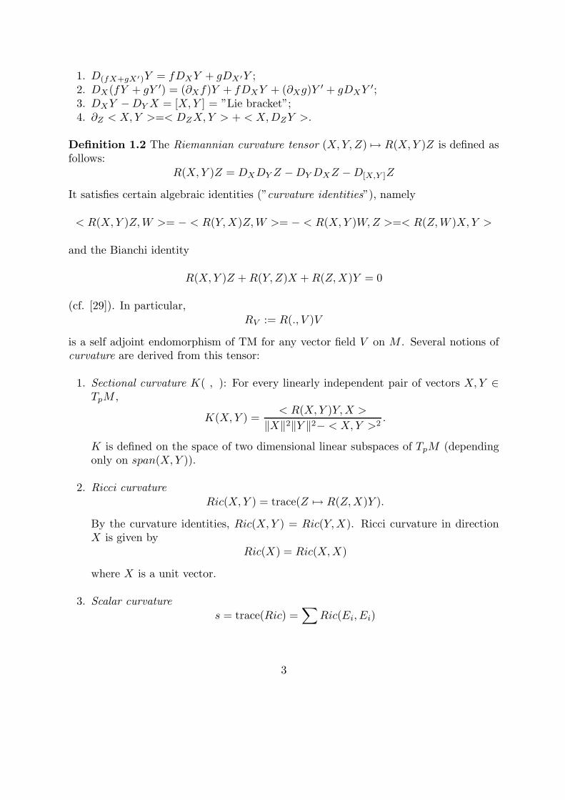
1. D(fX+gX′)Y = fDXY + gDX′Y ;2. DX(fY + gY ′) = (∂Xf)Y + fDXY + (∂Xg)Y

′ + gDXY′;

3. DXY −DYX = [X,Y ] = ”Lie bracket”;4. ∂Z < X, Y >=< DZX,Y > + < X,DZY >.

Definition 1.2 The Riemannian curvature tensor (X,Y, Z) 7→ R(X,Y )Z is defined asfollows:

R(X,Y )Z = DXDY Z −DYDXZ −D[X,Y ]Z

It satisfies certain algebraic identities (”curvature identities”), namely

< R(X,Y )Z,W >= − < R(Y,X)Z,W >= − < R(X,Y )W,Z >=< R(Z,W )X,Y >

and the Bianchi identity

R(X,Y )Z + R(Y, Z)X + R(Z,X)Y = 0

(cf. [29]). In particular,RV := R(., V )V

is a self adjoint endomorphism of TM for any vector field V on M . Several notions ofcurvature are derived from this tensor:

1. Sectional curvature K( , ): For every linearly independent pair of vectors X,Y ∈TpM ,

K(X,Y ) =< R(X,Y )Y,X >

‖X‖2‖Y ‖2− < X, Y >2.

K is defined on the space of two dimensional linear subspaces of TpM (dependingonly on span(X,Y )).

2. Ricci curvatureRic(X,Y ) = trace(Z 7→ R(Z,X)Y ).

By the curvature identities, Ric(X,Y ) = Ric(Y,X). Ricci curvature in directionX is given by

Ric(X) = Ric(X,X)

where X is a unit vector.

3. Scalar curvatures = trace(Ric) =

∑

Ric(Ei, Ei)

3

where {Ei}ni=1 is a local orthonormal basis.

There is a close relationship between RV = R(., V )V and the sectional curvature:Let ‖V ‖ = 1. For X orthogonal to V we have

< RVX,X >=< R(X,V )V,X >= K(V,X)‖X‖2

Hence the highest (”λ+”) and lowest (”λ−”) eigenvalues of RV give a bound toK(V,X),since

λ−(RV ) ≤ < RVX,X >

< X,X >≤ λ+(RV ).

Moreover, trace(RV ) = Ric(V, V ).

Let us come back to the covariant derivative. It is easy to see that for any p ∈M ,(DXY )p depends only on dYp.X(p) where the vector field Y is considered as a smoothmap Y : M → TM . Therefore, the covariant derivative is also defined if the vectorfields X and Y are only partially defined. E.g. if γ : I → M is a smooth regular curveand Y is a vector field along γ, i.e. a smooth map Y : I → TM with

Y (t) ∈ Tγ(t)M

for all t ∈ I (e.g. γ′ is such a vector field), then

Y ′(t) :=DY (t)

dt:= Dγ′(t)Y

is defined (just extend γ′ and Y arbitrarly outside γ). Similar, if γ : I1 × ...× Ik →Mdepends on k variables, we have k partial derivatives ∂γ

∂tiand corresponding covariant

derivatives D∂ti

(i = 1, ..., k) along γ. (Formally, a vector field along γ is a section of thepull-back bundle γ∗TM , and D induces a covariant derivative on this bundle.)

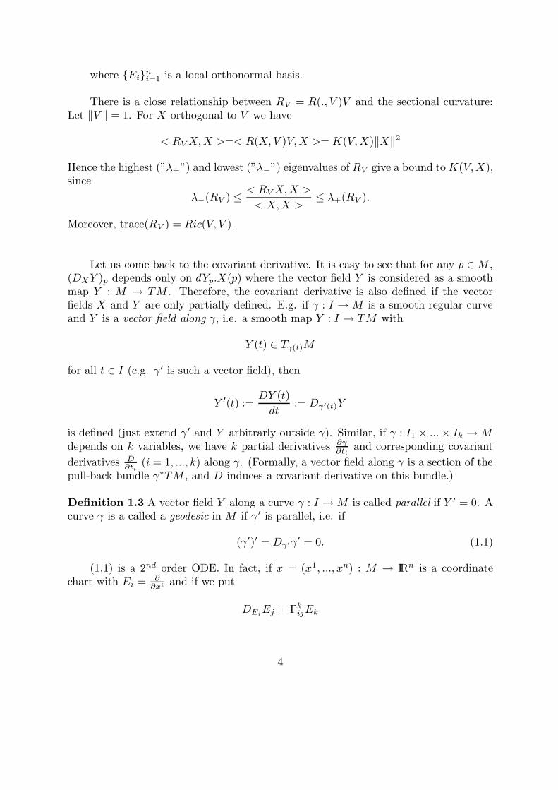
Definition 1.3 A vector field Y along a curve γ : I →M is called parallel if Y ′ = 0. Acurve γ is a called a geodesic in M if γ ′ is parallel, i.e. if

(γ′)′ = Dγ′γ′ = 0. (1.1)

(1.1) is a 2nd order ODE. In fact, if x = (x1, ..., xn) : M → IRn is a coordinatechart with Ei = ∂

∂xi and if we put

DEiEj = ΓkijEk

4

(summation convention!), then γ ′ = (γi)′Ei where γi := xi ◦ γ, and

D

dtγ′ = (γi)′′Ei + (γj)′Dγ′Ej

withDγ′Ej = γkDEk

Ej = (γk)′ΓikjEi,

hence (1.1) is equivalent to

(γi)′′ + (γj)′(γk)′Γikj = 0

To some extent, Riemannian geometry is the theory of this ODE.

Definition 1.4 For any v ∈ TM let γv denote the unique geodesic with γ ′(0) = v. Fors, t ∈ IR with |s| and |t| small we have γsv(t) = γv(st) by uniqueness for ODE’s. Thusfor v ∈ TM with ‖v‖ small enough,

exp(v) := γv(1)

is defined and gives a smooth map exp : (TM)0 →M where (TM)0 is a neighborhoodof the zero section of TM . This is called the exponential map of M . M is called(geodesically) complete if exp is defined on all of TM . Fixing p ∈ M , we put expp =exp |TpM .

Remark 1.5 The map expp is a diffeomorphism near the origin (in fact, d(expp)0 isthe identity on TpM), and it maps all the lines through the origin of TpM onto thegeodesics through the point p ∈ M . Thus, expp : TpM → M can serve a a coordinatemap near p (”exponential coordinates”) which preserves the covariant derivative at p, i.e.covariant differentiation at p is the same as taking the ordinary derivative at 0 ∈ TpM inexponential coordinates. To see this, identify M and TpM near p via expp and considerthe ordinary derivative Do = ∂ on TpM . It satisfies the rules (1.),(2.) and (3.) of theLevi-Civita derivative (but not 4. for the Riemannian metric). Hence the differenceΓ = D − ∂ is a tensor field, i.e. ΓXfY = fΓXY for all functions f (by 2.), further it issymmetric, i.e. ΓXY = ΓYX (by 3.), and it satisfies Γvv = 0 for all v ∈ TpM , since Dand ∂ have the same geodesics at p. Thus Γ|p = 0.

5

2. Jacobi and Riccati equations; equidistant hypersurfaces.

Equation (1.1) is a nonlinear ODE which in general cannot be solved explicitly.Therefore, we consider its linearization. This is the ODE satisfied by a variation ofsolutions of (1.1), i.e. of geodesics. So let γ(s, t) = γs(t) be a smooth one-parameterfamily of geodesics γs. Put V = ∂γ

∂t∈ X(γs) and J = ∂γ

∂s. Then J is the variation vector

field and V the tangent field of the geodesics γs, hence DV V = O.

Fig. 1.

Then we have

J ′′ =D

∂t

D

∂tJ =

D

∂t

D

∂t

∂γ

∂s.

We can interchange the order of differentiation, getting

J ′′ =D

∂s

D

∂t

∂γ

∂t+R(V, J)V,

J ′′ +R(J, V )V = 0. (2.1)

Equation (2.1) is called Jacobi equation.

Definition 2.1 A vector field J along a geodesic γ is called a Jacobi field if it satisfiesthe Jacobi equation.

Remark 2.2 J is a Jacobi field along γ if and only if

J(t) =d

ds

∣

∣

∣

∣

0

γs(t) (2.2)

6

for some one-parameter family of geodesics γs with γ0 = γ.

Implication ”⇐” was shown above. To prove the opposite implication, we have toconstruct the family γs. Let α(s) = expγ(0) sJ(0). Let X be a vector field along α suchthat X(0) = γ′(0) and X ′(0) = J ′(0) and put

γs(t) = expα(s) tX(s) (2.3).

If we put

J =∂

∂s

∣

∣

∣

∣

0

γs,

then, by ”⇐”, J satisfies the Jacobi equation. Since J(0) = J(0) and

J ′(0) =D

∂t

∂

∂sγ|(0,0) =

D

∂s

∂

∂tγ|(0,0) =

D

∂sX(s)|0 = X ′(0) = J ′(0),

we get J = J by uniqueness of the solution.

Next, we want to split this 2nd degree equation in a system of 1st degree equations.To do this, we embed the 1-parameter family of geodesics describing the Jacobi fieldinto an (n− 1)-parameter family. I.e. we choose a suitable smooth map

γ : S × I →M

where S is an (n − 1)-dimensional manifold, such that γs(t) = γ(s, t) is a geodesic forany s ∈ S. If γ is a regular map, then V = dγ( ∂∂t ) can be viewed as a vector field on anopen subset of M with DV V = 0, and the Jacobi fields J arising from variations in S-directions commute with V , i.e. we have [J, V ] = 0 or

DV J = A · J (2.4)

where A = DV , i.e. A ·X = DXV . This is the first of our equations: Knowing A, werecieve J by solving a 1st order equation.

It remains to derive an equation for A. Let us consider first an arbitrary vectorfield V on M and let A = DV as before. In general, the covariant derivative of a tensorfield A is defined by

(DV A)X = DV (AX) −A ·DV (X).

7

Hence we have

(DVA)X = DVDXV − A(DXV + [V,X])

= DXDV V + R(V,X)V +D[V,X]V − A2X − A[V,X]

= DXDV V + RV (X) −A2X

.

ThereforeDV A+A2 +RV = D(DV V ). (2.5)

If we suppose DV V = 0 (i.e. the integral curves γs are geodesic), then we get an ODEfor A, the so called Riccati equation

A′ + A2 + RV = 0.

Thus we have split the Jacobi equation J ′′ = −RV J in two equations as follows:

J ′ = AJ (2.6)

A′ + A2 + RV = 0. (2.7)

We note that the second equation can be solved independently of the first.

Let us consider now the important special case where (DV )∗ = DV , that is

< DXV, Y >=< X,DY V >

for all vector fields X,Y . Then V is locally a gradient, i.e. locally V = ∇f for somefunction f : M → IR. Consequently, < V, V > is constant, since

∂X < V, V >= 2 < DXV, V >= 2 < DV V,X >= 0.

Thus we may assume that < V, V >= 1. Now let us consider the level hypersurfaces

St = {x ∈ M : f(x) = t}.

Since V = ∇f 6= 0, the St are regular hypersurfaces and V |Stis the unit normal vector

field on St. Thus in this case, our (n− 1)-parameter family of geodesics γ : S × I →Mis given by

γ(s, t) = exp(t− t0)V (s)

8

where S = St0 for some t0 ∈ I, and f(γ(s, t)) = t, or in other words, St = φt(S) whereφt(s) := γ(s, t). Such a family of hypersurfaces St is called equidistant, and the functionf− t0 is called the signed distance function of the hypersurface S = St0 . In fact we have

|f(x) − t0| = |x, S| := infs∈S|x, s| (2.8)

for x in a small neighborhood of S. Namely, if c : [a, b] → γ(S× I) ⊂M is a curve withc(a) ∈ St0 and c(b) ∈ St1 , then we have c(u) = γ(s(u), t(u)) with t(a) = t0, t(b) = t1,and

‖c′(u)‖2 = ‖dγ.s′(u)‖2 + t′(u)2 ≥ t′(u)2,

hence its length is

L(c) ≥∫ b

a

|t′(u)|du ≥ |t(b) − t(a)| ≥ |t0 − t1|.

Fig. 2.

In this case, all the quantities discussed above have geometric meanings. TheJacobi fields J(t) = dγ(s,t)(x, 0) = dφtx for x ∈ TsS measure the change of the metric ofSt = φt(S) when t is changed; in fact, ‖J(t)‖/‖J(t0)‖ is the length distortion betweenSt and S. Moreover, A = DV , restricted to the hypersurface St, is the shape operatorof St since V |St is a unit normal vector field on St. Its eigenvalues are called principalcurvatures, their average the mean curvature of St. Since Equation (2.7) is nonlinear,A(s, t) can develop singularities which are called focal points of S. Let us see someexamples.

Example 2.3 Let St = ∂Bt(p), where Bt(p) = {x ∈ M : |x, p| < t} is the Riemannianball.

9

Then V is radial and

A(t) ∼ 1

tI as t→ 0 (2.9)

because a Riemannian manifold behaves as a Euclidian space for t→ 0.

Example 2.4 ([9]) Let us suppose that RV = kI, k ∈ IR, that is M has constantcurvature. Moreover let us suppose that A = aI, where a is a real function defined onM (A is the second fundamental form of a family of umbilical hypersurfaces). In thiscase equation (2.7) becomes:

a′ + a2 + k = 0.

If k > 0, then M is a sphere (if it is assumed to be complete and simply connected).The solutions are given by

a(t) =√k cot(

√k(t− t0)).

This corresponds to the fact that there is (up to congruence) only one equidistantfamily of umbilical hypersurfaces in the sphere, namlely concentric Riemannian spheres(latitude circles).

Fig. 3.

If k = 0, then M is a Euclidean space and the solutions are

a(t) =1

(t− t0), a(t) = 0.

10

Fig. 4.

These solutions correspond to the three umbilical parallel hypersurface families in eu-clidean space: concentric spheres with increasing (t > t0) or decreasing (t < t0) radiiand parallel hyperplanes.Finally, if k < 0, the space M is hyperbolic. The solutions are given by

a(t) =√

|k| coth(√

|k|(t− t0), a(t) =√

|k| tanh(√

|k|(t− t0), a(t) = ±√

|k|.

These solutions correspond to the five families of equidistant hypersurfaces in the hy-perbolic space: Concentric spheres with increasing (t > t0) or decreasing (t < t0) radii,hypersurfaces which are parallel to an (n − 1)-dimensional hyperbolic subspace, andexpanding (t > t0) or contracting (t < t0) horospheres.

Fig. 5.

11

3. Comparison theory.

We want to derive a comparison theorem for solutions of the Riccati equationA′ + A2 + RV = 0 (cf. 2.7). Fixing an integral curve γ of V (which is a geodesic) andidentifying all tangent spaces Tγ(t)M by parallel displacement (i.e. via an orthonormalbasis (Ei(t)) of vector fields along γ which are parallel, i.e. E ′

i = 0), we consider A(t)as a self adjoint endomorphism on a single vector space E = Tγ(0)M . More generally,let E be a finite-dimensional real vector space with euclidean inner product 〈 , 〉. Thespace S(E) of self adjoint endomorphisms inherits the inner product

〈A,B〉 = trace(A ·B) (3.1)

for A,B ∈ S(E). We get a partial ordering ≤ on S(E) by putting A ≤ B if 〈Ax, x〉 ≤〈Bx, x〉 for every x ∈ E.

Theorem 3.1 (cf. [14], [9]) Let R1, R2 : IR → S(E) be smooth with R1 ≥ R2. Fori ∈ {1, 2} let Ai : [t0, ti) → S(E) be a solution of

A′i +A2

i +Ri = 0 (3.2)

with maximal ti ∈ (t0,∞]. Assume that A1(t0) ≤ A2(t0). Then t1 ≤ t2 and A1(t) ≤A2(t) on (t0, t1).

Proof. Let U = A2 − A1; then U(t0) ≥ 0 and

U ′ = A′2 − A′

1 = A21 −A2

2 +R1 − R2. (3.3)

We define S = R1 −R2 ≥ 0 and X = − 12(A1 +A2); the equation (3.3) takes the form

U ′ = XU + UX + S. (3.4)

We solve (3.4) by the variation of constant method (see [14], pag. 211, Remark 1). Lett′ = min{t1, t2} and g : (t0, t

′) → S(E) be a non-singular solution of the homogeneousequation

g′ = Xg. (3.5)

Now a solution U of (3.4) is obtained as

U = g · V · gT

where V verifiesV ′ = g−1 · S · (g−1)T . (3.6)

¿From S ≥ 0 we get V ′ ≥ 0; this, combined with V (0) ≥ 0, implies that V ≥ 0 andhence U ≥ 0. Thus A1 ≤ A2 on (t0, t

′). Since A′i is bounded from above, a singularity

can only be negative (going to −∞). So A1 ≤ A2 implies t′ = t1 ≤ t2.

12

Remark 3.2 Theorem 3.1 still holds if A1, A2 are singular at t0, but U = A2 −A1 hasa continuous extension to 0 with U(0) ≥ 0. See [14] for the proof. A similar argumentalso shows that t1 < t2 if A1(t0) < A2(t0); for a different proof of this fact see [11],Lemma 3.1.

The geometric interpretation of Theorem 3.1 is: principal curvatures (i.e. eigenvalues ofthe shape operator) of equidistant hypersurfaces decrease faster on the space of largercurvature. In particular, this is true for Riemannian spheres, as follows by Remark 3.2).

Now we want to find a comparison theorem for equation (2.6). For A ∈ S(E),denote by λ−(A) the lowest eigenvalue and by λ+(A) the highest eigenvalue of A.

Theorem 3.3 Let A1, A2 : (t0, t′) → S(E) such that

λ+(A1(t)) ≤ λ−(A2(t)) everywhere. (3.7)

Let J1, J2 : (t0, t′) → E be nonzero solutions of J ′

i = Ai · Ji. Then ‖J1‖/‖J2‖ ismonotoneously decreasing.Moreover, if

limt↘t0

‖J1‖‖J2‖

(t) = 1, (3.8)

then ‖J1‖ ≤ ‖J2‖.Equality holds at some t ∈ (t0, t

′) iff for i = 1, 2 we have Ji = j · vi on [t0, t] for someconstant vector vi ∈ E with Avi = λ · vi and j′ = λ · j, where λ = λ+(A1) = λ−(A2).

Proof. Since ‖Ji‖ is smooth, we can consider

‖Ji‖′‖Ji‖

=< J ′

i , Ji >

‖Ji‖2=< AiJi, Ji >

< Ji, Ji >∈ [λ−(Ai), λ+(Ai)]

so that

log(‖J1‖)′ =‖J1‖′‖J1‖

≤ λ+(A1) ≤ λ−(A2) ≤‖J2‖′‖J2‖

= log(‖J2‖)′,

hence(

log‖J1‖‖J2‖

)′≤ 0

which implies that ‖J1‖/‖J2‖ is monotoneously decreasing.If ‖J1‖/‖J2‖ has the same value 1 at t0 and t, then ‖J1‖ = ‖J2‖ on [t0, t] and we recieveJ ′i = AiJi = λJi from which the conclusion follows.

13

We consider the most important special cases due to Rauch and Berger (calledRauch I and Rauch II in [5]):

Rauch I

Suppose that Ji for i = 1, 2 are solutions of J ′′i + RiJi = 0 with λ−(R1) ≥ λ+(R2) and

Ji(0) = 0, ‖J ′1(0)‖ = ‖J ′

2(0)‖.Then ‖J1‖ ≤ ‖J2‖ up to the first zero of J1.

Rauch II

Suppose that Ji for i = 1, 2 are solutions of J ′′i + RiJi = 0 with λ−(R1) ≥ λ+(R2) and

J ′i(0) = 0, ‖J1(0)‖ = ‖J2(0)‖.

Then ‖J1‖ ≤ ‖J2‖ up to the first zero of J1.

In fact we apply the theorems 3.1 and 3.3 where in the first case, Ai(t) ∼ t−1I ast→ 0 and in the second case, Ai(0) = 0.

Corollary 3.4 Let M be a complete manifold with K ≥ 0, p0, p1 ∈M and γ : [0, 1] →M a shortest geodesic segment connecting p0 and p1. Let X⊥γ′ be a parallel vectorfield along γ. Put ps(t) = exp tX(s) for all s ∈ [0, 1]. Then

|p0(t), p1(t)| ≤ |p0, p1|with equality for some t > 0 only if p0, p1, p1(t), p0(t) bound a flat totally geodesicrectangle.

Proof. We have

|p0(t), p1(t)| ≤∫ 1

0

‖ ∂∂sps(t)‖dt

and Js(t) = ∂∂sps(t) is a Jacobi field along the geodesic γs(t) = ps(t) with J ′

s(0) = 0.Thus comparing with the euclidean case we get from Rauch II that ‖Js(t)‖ ≤ ‖Js(0)‖which shows the inequality. If we have equality at t1 > 0, the equality discussion ofTheorem 3.3 shows that Js is parallel along γs|[0, t1]. Moreover, the curves s 7→ ps(t) areshortest geodesics of constant length for 0 ≤ t ≤ t1. Thus the surface p : (s, t) 7→ ps(t)is a flat rectangle in M with

D

∂s

∂p

∂s=D

∂t

∂p

∂s=D

∂t

∂p

∂t= 0,

so it is also totally geodesic, i.e. covariant derivatives of vector fields tangent to p remaintangent to p.

14

4. Average comparison theorems.

Now we consider the trace of the Riccati equation A′ +A2 +RV = 0 for self adjointA. Since trace and derivative commute, we get

trace(A)′ + trace(A2) + Ric(V ) = 0. (4.1)

This is unfortunately not a differential equation for trace(A), because of the termtrace(A2). However, put

a =trace(A)

n− 1.

(Note that A(V ) = DV V = 0, so we consider A as an endomorphism on the (n − 1)-dimensional subspace E = V ⊥ of the tangent space.) Then

A = aI + A0,

with trace(A0) = 0, so A0 and I are perpendicular. Hence,

trace(A2) = ‖A‖2 = a2‖I‖2 + ‖A0‖2 = (n− 1)a2 + ‖A0‖2

and we get, from the trace equation (4.1):

a′ + a2 + r = 0 (4.2)

with

r =1

n− 1

(

‖A0‖2 +Ric(V ))

≥ 1

n− 1Ric(V ).

Geometric meaning: a(t) is the mean curvature of St.

Theorem 4.1 Suppose that A : [t0, t1) → S(E) (t1 ≤ +∞ maximal) is a solution of

A′ + A2 + R = 0 (4.3)

where R : IR → S(E) is given; suppose that for some constant k ∈ IR:

(1) trace(R) ≥ (n− 1)k(2) trace(A(t0)) ≤ (n− 1)a(t0)

where a : [t0, t2) → IR is a solution of

a′ + a2 + k = 0 (4.4)

15

with t2 ≤ +∞ maximal. Let

a =trace(A)

n− 1. (4.5)

Then t1 ≤ t2 and a(t) ≤ a(t) for t ∈ [t0, t1).

Proof. Apply theorem 3.1 with (R1, A1, R2, A2) replaced with (r, a, k, a).

Remark 4.2 By Remark 3.2, the theorem remains true if A(t) ∼ 1t−t0 I and a is the

solution of (4.4) with a pole at t0, i.e. a = s′/s, where s is the solution of

s′′ + ks = 0, s(t0) = 0, s′(t0) = 1.

Next, let J1, . . . , Jn−1 be a basis of solutions of J ′ = A · J , and put

j = det(J1, . . . , Jn−1).

Since

(J1 ∧ . . . ∧ Jn−1)′ =

n−1∑

k=1

J1 ∧ . . . ∧A · Jk ∧ . . . ∧ Jn−1,

we getj′ = (n− 1)a · j. (4.6)

Geometrically, equation (4.6) says how the volume element of St, namely det(dφt) (seepage 9 of chapter 2), changes with t.

Theorem 4.3 Let A : [t0, t1) → S(V ) be given with

a ≤ a,

where a = 1n−1

trace(A), and let j be as above. Choose j such that

j′ = (n− 1)a · j.

Then j/j is monotonously decreasing.

Proof. Apply theorem 3.3 with (A1, J1, A2, J2) replaced with ((n− 1)a, j, (n− 1)a, j).

16

5. Bishop - Gromov inequality

Let M be a complete connected Riemannian manifold. By the theorem of Hopfand Rinow (cf. [29]), any two points p, q ∈ M can be connected by a shortest geodesicγ, i.e. L(γ) = |p, q|. Let SpM = {v ∈ TpM : ‖v‖ = 1} be the unit sphere in TpM . Forany v ∈ SpM , we define

cut(v) = max{t : γv|[0,t] is shortest}.

This defines a function cut : SpM → (0,∞], the cut locus distance, which is continuous(cf [5], p.94). Let

Cp = {tv : v ∈ SpM, t ≤ cut(v)}. (5.1)

This is a closed subset of TpM , and its boundary ∂Cp (sometimes also expp(∂Cp) ⊂M)is called the cut locus of the point p. It follows from this definition that

Br(p) = expp(Br(0)) = expp(Br(0) ∩ Cp) ∀r > 0. (5.2)

In fact, if we choose q ∈ Br(p), there exists a shortest geodesic γv joining p and q; thelength of γv should be ≤ cut(v), hence v ∈ Cp (theorem of Hopf - Rinow).

Example 5.1 On the unit sphere we have cut(v) = π for every v. In fact, in everydirection, the geodesic is a meridian, hence it is shortest up to the opposite (”antipodal”)point.

Example 5.2 On the cylinder S1 × IR, we have cut(v) = π/ cosα where α is the anglebetween v and the S1-direction.

Fig. 6.

17

There are two ways how a geodesic γ = γv : [0,∞) → M (where v ∈ SpM) cancease to be shortest beyond the parameter t0 = cut(v) (cf. [5], p.93): Either there existsa nonzero Jacobi field J along γ which vanishes at 0 and t0 - in this case, γ(t0) is calleda conjugate point of p (cf. Example 5.1), or there exists a second geodesic σ 6= γ ofthe same length which also connects p and γ(t0) (cf. Example 5.2). Hence q = γ(t0)is in the cut locus of p = γ(0) iff p is in the cut locus of q. Moreover, there are noconjugate points on γ|[0, cut(v)). The conjugate points in turn are the singular valuesof the exponential map expp; more precisely, we have:

Lemma 5.3 Let J(t) be the Jacobi field along γv defined by J(0) = 0, J ′(0) = w. Thenwe have

d(expp)tv.tw = J(t).

In particular, d(expp)tv is singular if and only if expp(tv) is a conjugate point of p.

Proof. Let w ∈ TvTpM ≡ TpM . Then we have

d(expp)v.w =d

ds

∣

∣

∣

∣

s=0

expp(v + sw) =d

ds

∣

∣

∣

∣

s=0

γv+sw(1). (5.3)

If we let

J(t) =∂

∂s

∣

∣

∣

∣

s=0

γv+sw(t), (5.4)

then J is the Jacobi field along γv with initial conditions J(0) = 0 and

J ′(0) =D

∂t

∣

∣

∣

∣

0

∂

∂s

∣

∣

∣

∣

0

γv+sw(t)

=D

∂s

∣

∣

∣

∣

0

∂

∂t

∣

∣

∣

∣

0

γv+sw(t)

=D

∂s

∣

∣

∣

∣

0

(v + sw) = w

.

Therefore we get

d(expp)v · w = J(1), (5.5)

and generally

d(expp)tv · tw = J(t). (5.6)

18

Remark 5.4 Consequently, on the interior of Cp, the exponential map expp is injectiveand regular, hence a diffeomorphism. Note that Int(Cp) is star-shape, thus it is con-tractive; hence also its image is contractive. But by Hopf-Rinow, the whole manifoldM is the image of expp : Cp → M , so the topology of M is given by the image of theboundary ∂Cp.

After these preparations, we come to the main theorem of this section.

Theorem 5.5 Let us consider a manifold Mn with Ricci curvature satisfying

Ric

n− 1≥ k.

Let M be the complete simply connected n-manifold with constant curvature k (standardspace of constant curvature k) and Br ⊂ M the ball of radius r in M . Then, for allp ∈M , we have that

VolBr(p)

VolBr↘r (5.7)

i.e. this quotient is monotonely decresing with r. Moreover, for r → 0, the quotientgoes to one.

Corollary 5.6 For any two positive real numbers R > r we have

VolBR(p)

VolBr(p)≤ VolBR

VolBr. (5.8)

Remark 5.7 Corollary 5.6 gives an upper bound for the growth of the metric balls inM . Moreover, if equality holds for some r < R, then BR(p) is isometric to Br (this canbe seen from the proof).

Proof of the theorem. By (5.3) we have

VolBr(p) =

∫

Br(0)∩Cp

det(

d(expp)u)

du. (5.9)

Passing to polar coordinates and denoting r(v) = min{r, cut(v)}, we get

VolBr(p) =

∫

S

∫ r(v)

0

det(

d(expp)tv)

tn−1dt dv (5.10)

19

where S := S1(0) ⊂ TpM . If we consider a basis e1, . . . , en−1 of v⊥ ⊂ TpM , then byLemma 5.3,

d(expp)tvei =1

td(expp)tvtei =

1

tJi(t),

where Ji is the Jacobi field along γv with Ji(0) = 0 and J ′i(0) = ei. Hence

det(

d(expp)tv)

=1

tn−1det (J1(t), . . . , Jn−1(t)) , (5.11)

and equation (5.10) becomes

VolBr(p) =

∫

S

∫ r(v)

0

jv(t)dt dv (5.12)

wherejv(t) = det (J1(t), . . . , Jn−1(t)) . (5.13)

If we put jv(t) = 0 for t > cut(v), then by the comparison theorem 4.3 we get

(jv/j) ↘

on [0, r] and hence

q :=1

Vol(S)

∫

S

(jv/j)dv

is still monotone. Moreover,

VolBr =

∫

S

∫ r

0

j(t)dtdv = Vol(S)

∫ r

0

j(t)dt. (5.14)

Therefore we have thatVolBr(p)

VolBr=

∫ r

0q(t)j(t)dt

∫ r

0j(t)dt

(5.15)

is a monotone decreasing function in r, because the mean of a monotone function ongrowing intervals is still monotone.

If r → 0, both volumes approximate the euclidean ball volume, hence the quotientgoes to one.

20

6. Toponogov’s Triangle Comparison Theorem

Let us fix o ∈ M and let ρ = |o, ·|. We already know that near o, precisely inexpo(Int(Co)\{0}), ρ is a C∞ function and

ρ(expo(v)) = ‖v‖. (6.1)

Let us consider the unit radial field V = ∇ρ. Then Sr = ∂Br(o) is a family of equidistanthypersurfaces, as in chapter 2.

Suppose that the sectional curvature K of M is ≥ k. If M is the standard space ofsectional curvature k, then, by the comparison theorem 3.1, we get

A ≤ A =s′

sI, (6.2)

where s is a solution of s′′ + ks = 0 with initial dates s(0) = 0, s′(0) = 1, and A =DV = D∇ρ is the Hessian of ρ. (Recall from Example 2.4 that a = s′/s is the (unique)solution of the equation a′ + a2 + k = 0 with a pole at t = 0.)

Therefore,

D∇ρ|V ⊥ ≤ s′

sI, (6.3)

whileD∇ρ|IRV = 0, (6.4)

because ρ grows linearly along the integral curves of V . Analogous relations hold for ρ:

D∇ρ|V ⊥ =s′

sI (6.5)

D∇ρ|IRV = 0 (6.6)

Now we want to find a unique estimate for the whole Hessian. To get this we modify ρ(and analogously ρ) suitably: Consider σ = f ◦ ρ, where f : IR → IR is a function yet tobe determined. Then

D∇(f ◦ ρ) = D ((f ′ ◦ ρ)∇ρ) = f ′′(ρ)dρ · ∇ρ+ f ′(ρ)D∇ρ. (6.7)

On V ⊥ we have f ′′(ρ)dρ · ∇ρ = 0 and D∇ρ ≤ (s′/s)I; while f ′′(ρ)dρ · ∇ρ = f ′′(ρ)I andD∇ρ = 0 on IR · V . If we choose f as a principal function of s, i.e. f ′ = s, then we get

f ′′(ρ) = −kf(ρ) + C,

hence (6.3) and (6.4) giveD∇σ ≤ −kσI + C (6.8)

21

where C is some fixed constant. Analogously, for σ = f ◦ ρ, we get from (6.5) and (6.6)

D∇σ = −kσI + C. (6.9)

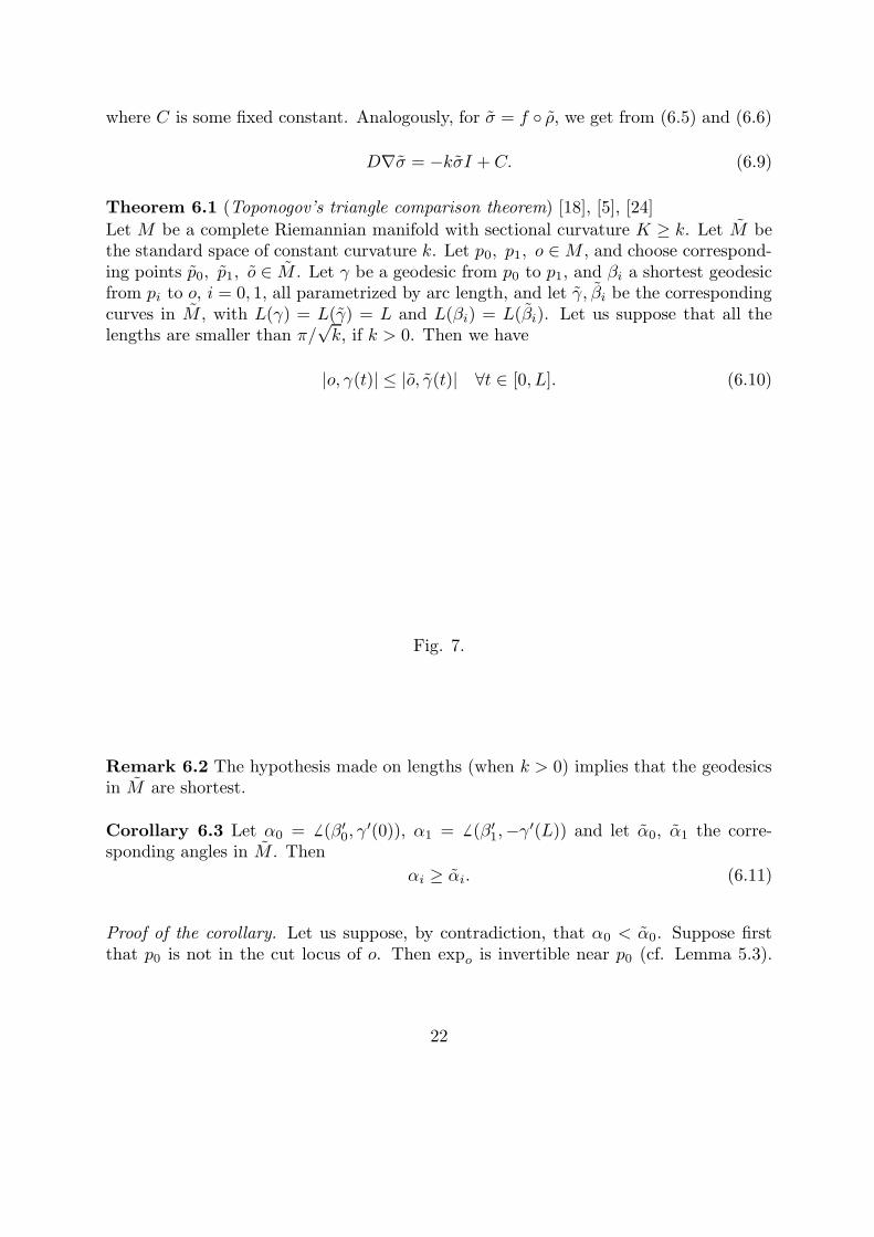
Theorem 6.1 (Toponogov’s triangle comparison theorem) [18], [5], [24]

Let M be a complete Riemannian manifold with sectional curvature K ≥ k. Let M bethe standard space of constant curvature k. Let p0, p1, o ∈M , and choose correspond-ing points p0, p1, o ∈ M . Let γ be a geodesic from p0 to p1, and βi a shortest geodesicfrom pi to o, i = 0, 1, all parametrized by arc length, and let γ, βi be the correspondingcurves in M , with L(γ) = L(γ) = L and L(βi) = L(βi). Let us suppose that all thelengths are smaller than π/

√k, if k > 0. Then we have

|o, γ(t)| ≤ |o, γ(t)| ∀t ∈ [0, L]. (6.10)

Fig. 7.

Remark 6.2 The hypothesis made on lengths (when k > 0) implies that the geodesicsin M are shortest.

Corollary 6.3 Let α0 = 6 (β′0, γ

′(0)), α1 = 6 (β′1,−γ′(L)) and let α0, α1 the corre-

sponding angles in M . Then

αi ≥ αi. (6.11)

Proof of the corollary. Let us suppose, by contradiction, that α0 < α0. Suppose firstthat p0 is not in the cut locus of o. Then expo is invertible near p0 (cf. Lemma 5.3).

22

Let βt be the shortest geodesic joining o to γ(t); the corresponding one βt is a shortestgeodesic in M (for t close to 0), hence

L(βt) ≥ |o, γ(t)|,

L(βt) = |o, γ(t)|.

We have

L(βt) = |o, p0| + td

dt

∣

∣

∣

∣

0

L(βt) + O(t2) (6.12)

L(βt) = |o, p0| + td

dt

∣

∣

∣

∣

0

L(βt) + O(t2) (6.13)

and, by the first variation formula for curves (cf. [5], p.5), we get

d

dt

∣

∣

∣

∣

0

L(βt) = − < γ′(0), β′0(0) >

d

dt

∣

∣

∣

∣

0

L(βt) = − < γ′(0), β′0(0) > .

Since we supposed α0 < α0, for small t we get L(γt) < L(γt), which implies

|o, γ(t)| ≤ L(γt) < L(γt) = |o, γ(t)|.

Thus, by Toponogov’s theorem, we get a contradiction.If p0 happens to be a cut locus point of o, we choose oε = β0(ε) on β0 close to

o. Then certainly p0 is not in the cut locus of oε. Now we put βt the broken geodesicβ|[0, ε] ∪ βε,t where βε,t denotes the shortest geodesic from oε to γ(t), and the sameargument holds.

Proof of theorem 6.1

Let us define ρ = |o, ·|, ρ = |o, ·|, and σ = f ◦ ρ , σ = f ◦ ρ. Consider the function

δ = σ ◦ γ − σ ◦ γ. (6.14)

Hence we have to prove that

δ ≥ 0 on [0, L]. (6.15)

23

Fig. 8.

We prove (6.15) by contradiction. Suppose that there is t ∈ [0, L] such that δ(t) < 0,and let m = min[0,L] δ(t) < 0.We choose k′ > k sufficiently close to k and τ > 0 such that

L <π√k′

− τ. (6.16)

It is easy to find a solution a0 of the equation a′′0 + k′a0 = 0, with a0(−τ) = 0 anda0|[0,L] ≤ m. Then there exists λ > 0 such that a = λa0 satisfies the following proper-ties:

1. a ≤ δ2. a(t0) = δ(t0) for some t0 ∈ (0, L).

Case 1: γ(t0) is not a cut locus point of o. Thus δ is of class C∞ in a neighborhood oft0 and

(σ ◦ γ)′′ =< Dγ′∇σ, γ′ >≤ −k(σ ◦ γ) + C, (6.17)

where the inequality follows from (6.8). By eqution (6.9) we get

(σ ◦ γ)′′ =< Dγ′∇σ, γ′ >= −k(σ ◦ γ) + C. (6.18)

Henceδ′′ ≤ −kδ. (6.19)

On the other hand a′′ = −k′a. Moreover, in t0 we have δ(t0) = a(t0) < 0, which implies

(δ − a)′′(t0) ≤ δ(t0)(k′ − k) < 0. (6.20)

This is a contradiction because δ − a takes a minimum at t0.

24

Case 2: γ(t0) is a cut locus point of o. Let β be a shortest geodesic from o to γ(t0). Wechoose oε on β close to o, say |oε, o| = ε. Then we replace ρ by ρε(x) := |x, oε|+ |oε, o|.By triangle inequality,

ρε(x) ≥ ρ(x), (6.21)

and equality holds at x = γ(t0). In other words, ρε is an upper support function of ρ atγ(t0). Since β is shortest from o to γ(t0), oε is not a cut point of γ(t0), and therefore,γ(t0) is not a cut point of oε (cf. Ch.5). Putting σε = f ◦ ρε, we get the same estimatesas in Case 1 for σε in place of σ, up to a small error which goes to zero as ε→ 0:

(σε ◦ γ)′′ ≤ −k(σε ◦ γ) + C + error. (6.22)

Now σε is an upper support function of σ at γ(t0) as f is monotoneously increasing.Hence δε− a is an upper support function of δ− a at t0 where δε = σε− σ. Thus it alsotakes a minimum at t0. But this is a contradiction, because (δε− a)′′(t0) < 0 by (6.20).

Remark 6.4 The above proof is essentially due to Karcher ([24]). Recently, M. Kurzel([27]) extended this proof to the case where curvature bounds are given which dependradially on the point (rather than being constant).

25

7. Number of generators and growth of the fundamental group

Let M be a complete Riemannian manifold and M its universal covering. Thefundamental group π1(M) will be viewed as group of deck transformations acting on M .In other words, M is the orbit space of a discrete group Γ ∼= π1(M) of isometries of Macting freely on M , i.e. if g ∈ Γ with g(p) = p for some p ∈M , then g = 1.

Remark 7.1 The fundamental group of any compact Riemannian manifold M is finitelygenerated.

Proof. There exists a compact fundamental domain F (see definition below) for theaction of Γ on M ; e.g. one may take the so called Dirichlet fundamental domain

F = {x ∈ M ; |x, o| ≤ |x, go| ∀g ∈ Γ}.

We say that g ∈ Γ is small if gF ∩ F 6= ∅, i.e. if the fundamental domains F andgF are neighbors. If d(F ) denotes the diameter of F , i.e. the largest possible distancewithin F , then gF ⊂ B2d(F )(o) for all small g, for some fixed o ∈ F . Since the subsetsg(Int(F )) are all disjoint with equal volume, there can be only finitely many of themin this ball, hence there exist only finitely many small g. We claim that they form aset of generators. In fact, let g ∈ Γ arbitrary. Choose a geodesic segment γ from o togo. Then γ is covered by finitely many fundamental domains g0F, ..., gNF where g0 = 1and gN = g, and gi−1F , giF are neighbors. Thus g−1

i gi−1 is small, and hence g is acomposition of small group elements.

Definition 7.2 A closed subset F ⊂ M is a fundamental domain for a group Γ actingon M if(a.) Int(F ) ∩ Int(gF ) = ∅ ∀g 6= 1;(b.) Γ · F = M .

For a noncompact manifold M , the fundamental group may have infinitely manygenerators. The next theorem shows that this does not happen if M has K ≥ 0; in fact,there is an a-priori bound on the number of generators, i.e. the cardinality of a suitablychosen set of generators:

Theorem 7.3 (Gromov 1978, cf [24])There exists a number c(n) such that:(a) the number of generators for π1(M) is ≤ c(n) for any n-dimensional complete

manifold M with curvature K ≥ 0.(b) the number of generators for π1(M) is ≤ c(n)1+kD for any n-dimensional compact

manifold M with curvature K ≥ −k2 and diameter bounded, diam(M) ≤ D.

26

Proof. We prove only part a); the second part is similar, but more technical (see Remarkat the end of the proof).We define a ”norm” in Γ as follows:

|g| = |p, g(p)|

for some fixed p ∈ M . There exists g1 ∈ Γ \ {1} with |g1| minimal (not necessarilyunique). By induction, we can construct a sequence (gj): given g1, . . . , gk, we define

Γk = 〈g1, . . . , gk〉 ⊂ Γ

and choose gk+1 ∈ Γ \ Γk such that |gk+1| has minimum norm in Γ \ Γk. To finish theproof, we only have to show

Claim: Γk = Γ for some k ≤ c0(n) := 2√

5n.

Proof of the claim: for j > i we have |gj| ≥ |gi|, and moreover

|gi(p), gj(p)| = |p, g−1i gj(p)| = |g−1

i gj | ≥ |gj|

since g−1i gj ∈ Γ \ Γj−1 (otherwise g−1

i gj, gi ∈ Γj−1 which would imply that gj ∈ Γj−1

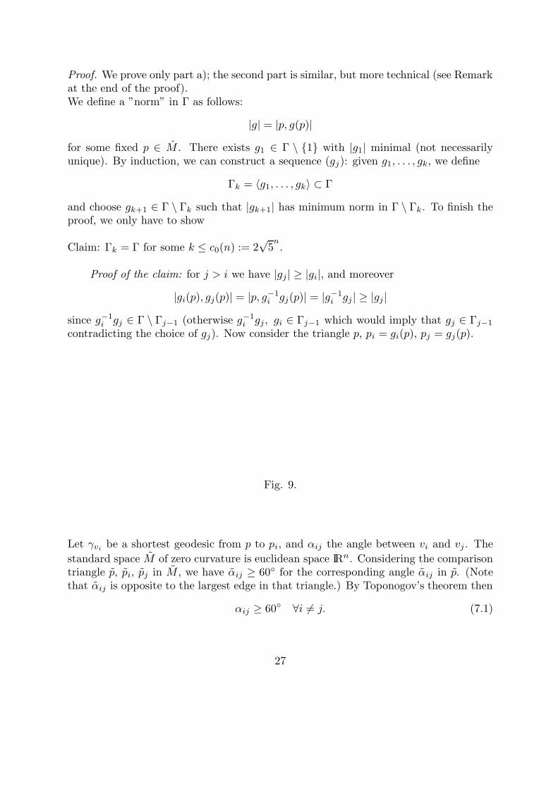
contradicting the choice of gj). Now consider the triangle p, pi = gi(p), pj = gj(p).

Fig. 9.

Let γvibe a shortest geodesic from p to pi, and αij the angle between vi and vj . The

standard space M of zero curvature is euclidean space IRn. Considering the comparisontriangle p, pi, pj in M , we have αij ≥ 60◦ for the corresponding angle αij in p. (Notethat αij is opposite to the largest edge in that triangle.) By Toponogov’s theorem then

αij ≥ 60◦ ∀i 6= j. (7.1)

27

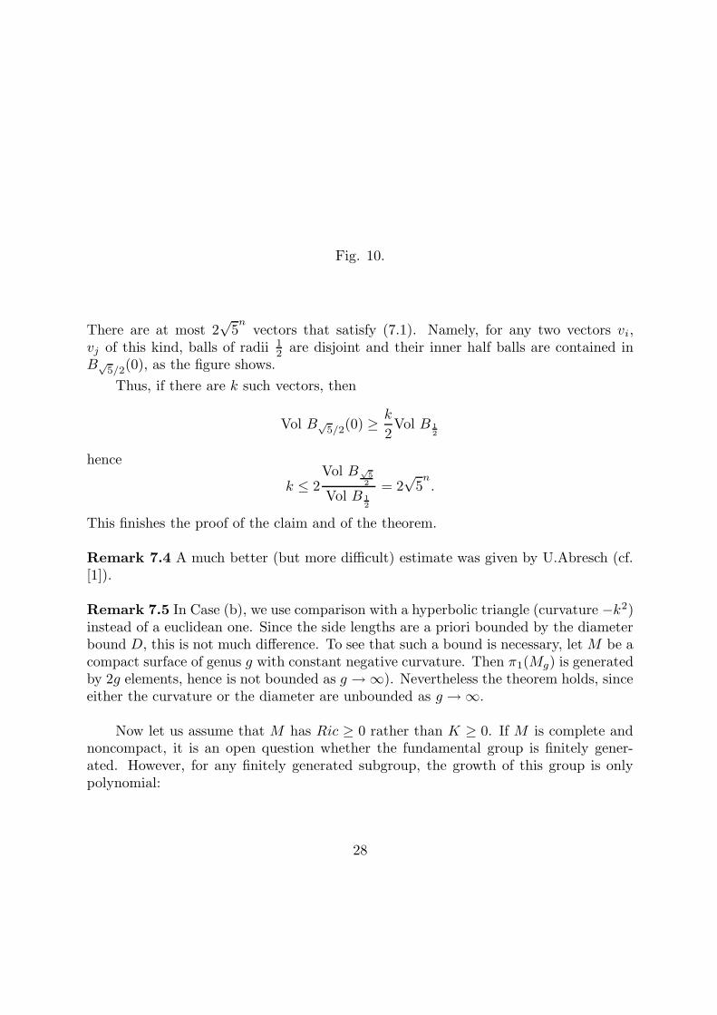
Fig. 10.

There are at most 2√

5n

vectors that satisfy (7.1). Namely, for any two vectors vi,vj of this kind, balls of radii 1

2 are disjoint and their inner half balls are contained inB√

5/2(0), as the figure shows.

Thus, if there are k such vectors, then

Vol B√5/2(0) ≥ k

2Vol B 1

2

hence

k ≤ 2Vol B√

5

2

Vol B 1

2

= 2√

5n.

This finishes the proof of the claim and of the theorem.

Remark 7.4 A much better (but more difficult) estimate was given by U.Abresch (cf.[1]).

Remark 7.5 In Case (b), we use comparison with a hyperbolic triangle (curvature −k2)instead of a euclidean one. Since the side lengths are a priori bounded by the diameterbound D, this is not much difference. To see that such a bound is necessary, let M be acompact surface of genus g with constant negative curvature. Then π1(Mg) is generatedby 2g elements, hence is not bounded as g → ∞). Nevertheless the theorem holds, sinceeither the curvature or the diameter are unbounded as g → ∞.

Now let us assume that M has Ric ≥ 0 rather than K ≥ 0. If M is complete andnoncompact, it is an open question whether the fundamental group is finitely gener-ated. However, for any finitely generated subgroup, the growth of this group is onlypolynomial:

28

Definition 7.6 Let Γ be a finitely generated group and G a finite set of generators ofΓ with G = G−1 and 1 ∈ G. We define the growth function N(k) (depending on Γ andG) as follows:

N(k) = ]{g ∈ Γ | ∃g1, . . . , gk ∈ G such that g = g1 · . . . · gk}. (7.2)

So N(k) is the number of group elements which can be written as a product of kelements of G. The dependence of N(k) on G is easy to estimate: If G′ is another suchgenerating set, then there are numbers p, q such that any element of G can be expressedby p elements of G′ and each element of G′ by q elements of G. Thus we have

N ′(k) ≥ N(qk), N(k) ≥ N ′(pk).

Theorem 7.7 (Milnor ’68, [30])Let M be a complete manifold with Ric ≥ 0 and let Γ ⊂ π1(M) any finitely generatedsubgroup of the fundamental group. Then the growth of Γ can be estimated by

N(k) < c · kn. (7.3)

where the constant c depends on M and the chosen set of generators of Γ.

Proof. Let G be a set of generators as above; it has N(1) elements. Fix a point o ∈ M .For all g ∈ Γ, let |g| = |o, go|. Put R′ = max{|g|; g ∈ G}. Choose some r > 0 smallenough, so that

Br(go) ∩ Br(o) = ∅ ∀g ∈ Γ \ {1} (7.4)

Put R = R′ + r. Then the family of balls {Br(go); g ∈ G} is disjoint and its union iscontained in BR(o) so that

Vol(

BR(o))

≥ N(1) · Vol(

Br(o))

. (7.5)

We can iterate this argument as follows: At the second step, we consider

G2 := {g1g2; g1, g2 ∈ G}.

with ](G2) = N(2). Then all balls Br(go) with g ∈ G2 are disjoint and contained inB2R(o) so that

Vol(

B2R(o))

≥ N(2) · Vol(

Br(o))

. (7.6)

In general, we obtain that

Vol(

BkR(o))

≥ N(k) · Vol(

Br(o))

. (7.7)

29

Recall that we have the Bishop - Gromov inequality (cf. Corollary 5.6),

Vol(

BkR(o))

≤ ωnknRn,

where ωn denotes the volume of the euclidean unit ball, hence

N(k) ≤{

ωnRn

Vol(

Br(o))

}

kn. (7.8)

30

8. Gromov’s estimate of the Betti numbers

Homology is a main tool to measure the complexity of topology. Fix a field F andlet Hq(M) denote the q-th singular homology of M with coefficients in F. Further, letH∗(M) = ⊕q≥0Hq(M) be the total homology of M . The total Betti number of M isgiven by

b(M) = dimFH∗(M). (8.1)

Theorem 8.1 Gromov, 1980 (cf. [15], [1], [28])There is a constant C(n) such that:(a.) any complete n-dimensional manifold M with nonnegative curvature K satisfies

b(M) ≤ C(n); (8.2)

(b.) any compact n-dimensional manifold M with curvature K ≥ −k2, and boundeddiameter, diam(M) ≤ D, satisfies

b(M) ≤ C(n)1+kD. (8.3)

We will give the proof of part (a.), following ideas of Abresch [1] and W.Meyer[28]. (Part (b.) is similar, cf. Remark 7.2.) The proof uses the estimates of Bishop-Gromov and Toponogov. It can be viewed as an application of some sort of Morsetheory for the distance function ρ(x) = |o, x| where o ∈ M is fixed. In ordinary Morsetheory, one considers a smooth function f : M → IR with isolated critical points withnondegenerate Hessian (p critical means that ∇f(p) = 0), and one observes how thetopology of M c = {x ∈ M ; f(x) < c} is changed as c grows. There are two main factsin Morse theory (cf [29]):(1.) If M b \Ma contains no critical points, then M b and Ma are diffeomorphic.(2.) If M b \Ma contains exactly one critical point p, then M b is homotopic to Ma with

a k-cell attached, where k is the index of the Hessian of f at p.

The distance function ρ = |o, | : M → IR is no longer smooth, but we still have thenotions of critical and regular points:

Definition 8.2 A point x ∈ M is called a regular point of ρ if there exists v ∈ TxMsuch that

〈v, γ′(0)〉 < 0 (8.4)

for any shortest geodesic γ from x to o. Any such vextor v is called gradientlike.

31

A point x ∈M is a critical point for ρ if it is non-regular, i.e. if for any v ∈ TxM thereis a shortest geodesic γ from x to o such that

〈v, γ′(0)〉 ≥ 0.

Remark 8.3 These notions make sense also if the point o is replaced by a closed subsetΣ ⊂M . This will be needed in Ch.10.

Fact (1.) is still valid: Since the set of initial vectors of shortest geodesics to ois closed, the gradientlike vectors form an open subset of TM and moreover a convexcone at any regular point. Thus we may cover the closure of M b \Ma = Bb(o) \Ba(o)by finitely many open sets with gradientlike vector fields and past them together usinga partition of unity, thus getting a gradientlike vector field in a neighborhood of theclosure of Bb(o) \ Ba(o). This has the property that ρ is strictly increasing along itsintegral curves. Hence, pushing along the integral curves, we may deform the biggerball Bb(o) into the smaller one Ba(o). (See Lemma 10.9 for details.) We will use thisin Lemma 8.10 below.

However, Fact (2.) has no meaning and has to be replaced by another idea: Largeballs can be covered by a bounded number of small balls (Bishop-Gromov inequality),and the jump of the Betti number when passing from a small ball to a large ball can becontrolled using Toponogov’s theorem.

First of all, critical points of ρ are not necessarily isolated, but still in some sense,we have to take only finitely many into account:

Lemma 8.4 Let M be a complete manifold with nonnegative curvature. For any L > 1there exists a finite number c(n, L) such that there are at most c(n, L) critical points{qi} for ρ satisfying

|o, qi+1| ≥ L|o, qi|. (8.5)

E.g. for L = 2 we have c(n, 2) = 2√

5n.

Proof. Let (q1, q2, ...) be a maximal sequence satisfying (8.5). For i < j, let γ be ashortest geodesic from qi to qj and put v = γ′(0). Since qi is critical, there is a shortestgeodesic c from qi to o with the angle β = 6 (c′(0), v) ≤ 90◦. Applying Toponogov’stheorem (Corollary 6.3) with the standard space M = IRn, we get β ≤ 90◦.Consider first the limit case β = 90◦. Let α be the angle in o. It follows that

cos(α) =|qi, o||qj , o|

≤ 1

L.

32

Fig. 11.

Hence, if β ≤ 90◦,

αo ≥ arccos(1

L) =: α0.

Now we apply Toponogov’s theorem backwards for the angle at o, but this time weconsider an arbitrary shortest geodesic from qi to qj . Then for the angle α at o we have

α ≥ α ≥ α0.

It follows as in Ch.7 that there must be a finite number of such critical points. If L = 2,we have α0 = 60◦ and hence c(n, 2) = 2

√5n

as in the proof of Theorem 7.3.

Corollary 8.5 Given a complete manifold M with nonnegative curvature, all criticalpoints are contained in a finite ball.

Since we will work with many metric balls in M , we agree on the following conven-tion: If B = Br(p) be a fixed ball and λ > 0, we put λB := Bλr(p). More generally, forany q ∈M we let λB(q) := Bλr(q).

Definition 8.6 Let A ⊂ C ⊂ M . We define the content of A in C as the rank of theinclusion map on the homology level:

cont(A,C) = rk (i∗ : H∗(A) → H∗(C)) (8.6)

Then we define the content of a metric ball B as:

cont(B) = cont(B, 5B). (8.7)

33

Essentially, the content measures the total Betti number of a subset. But it is betterthan the Betti number since it has a nice monotonicity property: Note that if A ⊂ A′ ⊂B′ ⊂ B ⊂M then

cont(A,B) ≤ cont(A′, B′)

In the spirit of Morse theory, we will observe how the content of balls grows withthe radius. A measure for the number of critical points which are still outside the balland which will eventually increase the content is the corank. This definition involvesalso critical points of the distance function ρp = |p, | for points p ∈M different from o,called critical for p for short.

Definition 8.7 Let B = Br(o) a ball in M , r > 0. For p ∈ M , let k(r, p) be themaximum number of critical points q1, . . . , qk for p such that

1) |p, q1| ≥ 3Lr2) |p, qi+1| ≥ L|p, qi|.

By Lemma (8.3), k(r, p) ≤ c(L, n). Then we define the corank of B as follows:

corank(B) = inf{k(r, p) | p ∈ 5B}. (8.8)

Not all balls really contribute to the topology, namely the compressible ones:

Definition 8.8 A ball B ⊂ M is called compressible if there is B = 35B(q) for some

q ∈ 2B, and a diffeomorphism ϕ : M →M such that

ϕ|M\5B = id

andϕ(B) ⊂ B

For short: B is compressible into B. Otherwise, the ball B is called incompressible.

Lemma 8.9 Suppose that B is compressible into B, with B = 35B(p), and p ∈ 2B.

Thencont(B) ≥ cont(B) (8.9)

andcorank(B) ≥ corank(B). (8.10)

Proof. Let ϕ be the diffeomorphism which compresses B into B. From B ≈ ϕ(B) and

ϕ(B) ⊂ B ⊂ 5B ⊂ 5B, (8.11)

34

it follows that cont(B) ≥ cont(B).To show the second relation, put k = corank(B). Let p ⊂ 5B ⊂ 5B. Then there

are m ≥ k critical points q1, ..., qm for p with

|p, q1| ≥ 3Lr ≥ 3L · 3

5r, |p, qi+1| ≥ L|p, qi|.

Hence k( 35r, p) ≥ m ≥ k which shows corank(B) ≥ k.

Lemma 8.10 If B is incompressible, for any p ∈ 2B there is a critical point for p in5B \ B, where B = 3

5B(q).

Proof. Otherwise, we could deform B ⊂ 5B into B while keeping M \ 5B fixed, so Bwould be compressible.

Lemma 8.11 Let B be incompressible, and put B = λB(p) for some λ ≤ 15L and

p ∈ 32B. Then

corank(B) ≥ corank(B) + 1. (8.12)

Proof. Let p ∈ 32B and p ∈ 5B ⊂ 2B. By the previous lemma, there is a critical point

q0 for p in 3B(p) \ 35B(p), so we have

3r ≥ |p, q0| ≥3

5r ≥ 3Lλr. (8.13)

Now let k = corank(B). Then there are m ≥ k critical points q1, ..., qm for p with

|p, q1| ≥ 3Lr, |p, qi+1| ≥ L|p, qi|. (8.14)

Thus by (8.13),|p, q1| ≥ L|p, q0|, |p, q0| ≥ 3Lλr. (8.15)

Now (8.14) and (8.15) show

k(λr, p) ≥ m+ 1 ≥ k + 1.

Since p ∈ 5B was arbitrary, we get

corank(B) ≥ k + 1.

35

Proof of theorem 8.1

Let K = max{corank(B) | B ball in M}. By Lemma 8.4, K ≤ c(n, L), and by Corollary8.5, for a large enough ball B , there exists an isotopy of M that carries M into B,hence

cont(B) = cont(M,M) = b(M). (8.16)

Gromov’s theorem now follows if we prove that the content of any metric ball is boundedby a constant. This is done in 5 steps:

Step 1. If corank(B) = K then cont(B) = 1.Proof: Let p0 := p. By Lemma 8.11, B is compressible into B1 = 3

5B(p1) for somep1 ∈ 2B (otherwise, we could increase the corank). Hence, |p0, p1| < 2r. By Lemma8.9, corank(B1) = K and cont(B1) ≥ cont(B). Repeating the argument, we compressB1 (and hence B) into B2 = 3

5B1(p2) = ( 35 )2B(p2) for some p2 ∈ 2B1. Hence |p1, p2| <

35· 2r. After N steps, we have compressed B into BN = ( 3

5)NB(pN ) with |pi, pi+1| <

( 35)i · 2r for i = 0, ..., N . So we have for all q ∈ BN :

|p, q| <N

∑

i=0

(3

5)i · 2r < 5r.

Thus BN ⊂ 5B. Since the cut locus distance (injectivity radius) is bounded belowon the closure of B (by compactness), we find some N such that ( 3

5)Nr is smallerthan this bound which implies that BN is diffeormorphic to a euclidean ball and hencecontractible. So, cont(BN ) = 1 since b(BN ) = 1. On the other hand,

cont(BN ) ≥ cont(BN−1) ≥ ... ≥ cont(B)

which proves cont(B) = 1.

Step 2. Each ball B with cont(B) ≥ 2 is either incompressible or it contains anincompressible ball B with cont(B) ≥ cont(B) and corank(B) ≥ corank(B).Proof. Otherwise, we could use the process of Step 1 to show that cont(B) = 1.

Step 3. If B is incompressible, then any ball B = λB(p) with λ ≤ 15L and p ∈ 3

2Bsatisfies

corank(B) ≥ corank(B) + 1. (8.17)

Proof. Cf. Lemma 8.11.

Step 4. There is a number χ ≤ (2L)n(n+1)10n(n+1)(n+2) with the following property:Suppose that any ball B with corank(B) ≥ k has cont(B) ≤ ak. Then for any ball Bwith corank(B) ≥ k − 1 we have

cont(B) ≤ χ · ak (8.18)

36

Proof. By Step 2 we may assume that B is incompressible. Let λ = 1/(5L · 10n+1).We cover B with balls Bi = λB(pi) with pi ∈ B for i = 1, ..., N such that the balls12Bi are disjoint and inside B. Let 1

2B1 = 1

2λB(p1) the one of smallest volume among

12B1, ...,

12BN . Since B ⊂ 2B(p1), we have

vol(2B(p1)) ≥ vol(B) ≥N

∑

i=1

vol(1

2B1) ≥ N · vol(

1

2B1) = N · vol(

1

2λB(p1)).

On the other hand, by Bishop-Gromov (cf. Corollary 5.6),

vol(2B(p1))

vol( 12λB(p1)

) ≤ ωn · (2r)nωn · ( 1

2λr)n

= (4

λ)n,

thus

N ≤ (4

λ)n = (2L · 10n+2)n. (8.19)

By Step 3, all Bmi := 10mBi for m = 0, ..., n+1 have corank ≥ k and thus cont(Bi) ≤ ak.Since the radii of the Bi = B0

i are very small, we have (by triangle inequality)

B ⊂⋃

i

Bi ⊂⋃

i

10n+1Bi ⊂ 5B,

hencecont(B) ≤ cont(

⋃

i

Bi,⋃

i

10n+1Bi).

We will see below (cf. Appendix) that we may estimate

cont(⋃

i

Bi,⋃

i

10n+1Bi) ≤n+1∑

j=1

∑

i1<...<ij

cont(

j⋂

p=1

Bn−j+1ip

,

j⋂

p=1

10Bn−j+1ip

) (8.20)

where Bmi := 10mBi. Since

j⋂

p=1

Bmip ⊂ Bmi1 ⊂ 5Bmi1 ⊂j

⋂

p=1

10Bmip ,

we get

cont(

j⋂

p=1

Bmip ,

j⋂

p=1

10Bmip ) ≤ cont(Bmi1 ) ≤ ak.

37

There are N balls Bm1 , ..., BmN , so there are at most Nn intersections Bmi1 ∩ ... ∩ Bmij

where j = 1, ...n. Thuscont(B) ≤ Nn+1ak

which finishes the proof by (8.19)

Step 5. Let ak still denote an upper bound for the content of any ball with corank≥ k. By Step 1 we may choose aK = 1 where K ≤ c := c(L, n) is the biggest possiblecorank. Thus by Step 4, aK−1 = χ, hence aK−2 = χ2 and eventually (by induction),a0 = χK . Hence we get for any ball B

cont(B) ≤ χc

which finishes the proof since b(M) = cont(B) for some big ball (cf. (8.16)).

Remark 8.12 The highest known total Betti number for a manifold with K ≥ 0 is 2n,the total Betti number of the n-dimensional torus T n = S1 × ...× S1.

38

9. Convexity.

Definition 9.1 Let M be a Riemannian manifold. A continuous function f : M → IRis called convex if f ◦ γ : I → IR is convex for any geodesic γ : I → M , and f is calledconcave if −f is convex.

Theorem 9.2 A continuous function f : M → IR is convex if for any x ∈M and ε > 0there is a smooth lower support function fx,ε = f : Ux → IR (i.e., f ≤ f , f(x) = f(x)),

defined in a neighborhood Ux ⊂M , with D∇f(x) > −ε.

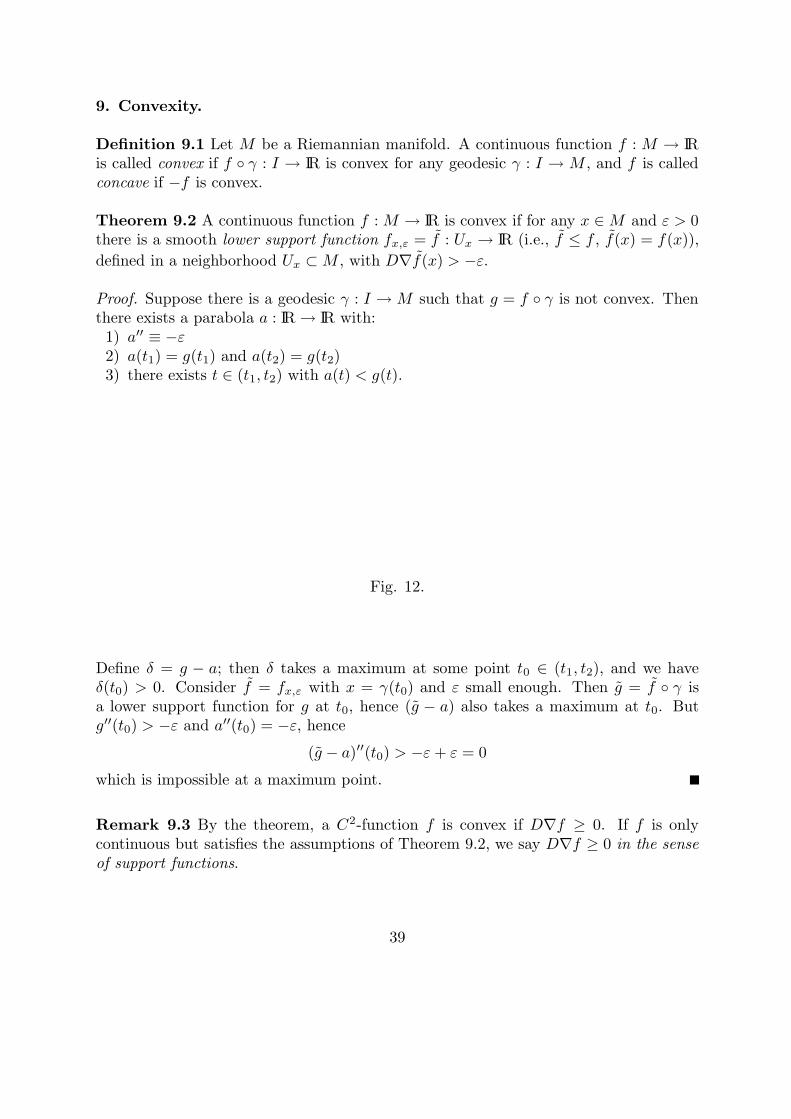
Proof. Suppose there is a geodesic γ : I → M such that g = f ◦ γ is not convex. Thenthere exists a parabola a : IR → IR with:1) a′′ ≡ −ε2) a(t1) = g(t1) and a(t2) = g(t2)3) there exists t ∈ (t1, t2) with a(t) < g(t).

Fig. 12.

Define δ = g − a; then δ takes a maximum at some point t0 ∈ (t1, t2), and we haveδ(t0) > 0. Consider f = fx,ε with x = γ(t0) and ε small enough. Then g = f ◦ γ isa lower support function for g at t0, hence (g − a) also takes a maximum at t0. Butg′′(t0) > −ε and a′′(t0) = −ε, hence

(g − a)′′(t0) > −ε+ ε = 0

which is impossible at a maximum point.

Remark 9.3 By the theorem, a C2-function f is convex if D∇f ≥ 0. If f is onlycontinuous but satisfies the assumptions of Theorem 9.2, we say D∇f ≥ 0 in the senseof support functions.

39

Example 9.4 Fix o ∈M and let ρ(x) = |o, x|. Then D∇ρ = A(ρ) > 0 for small ρ > 0 byexample 2.3. However, ρ is not smooth at o, but ρ2 is smooth (since ρ(expo(v))

2 = 〈v, v〉if ‖v‖ is small, cf. (6.1)), and it satisfies

D∇(ρ2) = 2(dρ · ∇ρ+ ρ ·D∇ρ) > 0,

hence ρ2 is convex near o.

Definition 9.5 A closed subset C ⊂ M is called convex if any geodesic segment γ inM with end points on C lies entirely in C. Clearly, if f : M → IR is a convex function,then the sublevel sets Ma = {x ∈M | f(x) ≤ a} are convex subsets for all a ∈ IR. Notethat the notion of convexity depends on the surrounding manifold. For example, in thecylinder S1 × IR with radius 1, a metric ball of radius r < π is not convex, but it isconvex in a slightly larger ball of radius r + ε < π inside the cylinder.

Definition 9.6 A smooth hypersurface S = ∂B ⊂ M is called convex hypersurface iffor the interior unit normal vector field N ,

DN ≤ 0. (9.1)

Clearly, if f is smooth and convex, then S = ∂Ma is a convex hypersurface unless a isa minimum of f (note that ∇f can vanish only at a minimum of a convex function f).Vice versa, if S = ∂B is a strictly convex hypersurface, i.e. DN < 0, then the signeddistance function ρ = ρS = ±| , S| is concave near S since DN is its Hessian along S(cf. Ch.2, p.9). Consequently, C = Clos(B) is convex in a neighborhood of C since itis a sublevel set of the convex function −ρ.

Theorem 9.7 Let B be compact and S = ∂B a convex hypersurface. If K ≥ 0 on B,then ρ = | , S| is concave on all of B.

Proof. Let x ∈ B and γ a shortest geodesic from x to S. Let p ∈ S be its endpoint.If we were in euclidean space, there would be a support hyperplane for B at p. In Mwe have a similar construction: For large R, let S = expp(∂BR(−RNp) ∩ U) where U

is a small neighborhood of −RNp in TpM . We will show that S supports B at p, i.e.

S∩B = ∅ and S∩∂B = {p}. To this end, we compare the signed distance functions ρ ofS and ρ of S near p. Since Np is a common normal vector for S and S, these functionsagree at p up to first derivatives. The second derivatives (Hessian) of ρ and ρ are givenby the shape operators A = (DN)p and A = (DN)p of S and S. By convexity, we have

A ≤ 0. On the other hand, A = 1R· I > 0. (In fact, this holds for the euclidean sphere

∂BR(−RNp) ⊂ TpM and hence also for S since expp preserves the covariant derivative

40

D at p, cf. Remark 1.5.) Thus A < A. However, the Hessians of ρ and ρ are bothzero in Np-direction, so we have no strict inequality. This can be repaired by passingto functions f ◦ ρ and g ◦ ρ which have the same level hypersurfaces as ρ and ρ, wherewe choose the functions f, g : IR → IR monotone with

f(0) = g(0), f ′(0) = g′(0), f ′′(0) < g′′(0).

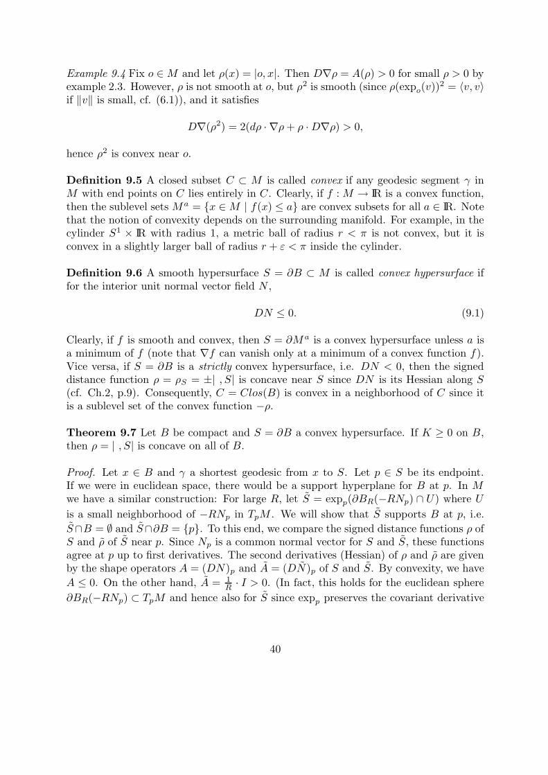
Then f ◦ ρ and g ◦ ρ agree at p up to first derivatives with Dd(f ◦ ρ)p < Dd(g ◦ ρ)p,so we get f ◦ ρ ≤ g ◦ ρ near p (in fact, ”<” outside p). In particular, the level setS = {g ◦ ρ = 0} lies outside B = {f ◦ ρ > 0}.

Fig. 13.

Now we consider the signed distance function ρ of S on its full domain, namelywherever the mapping

S × IR →M : (s, t) 7→ exp(tN(s))

is invertible, cf. Ch.2, p.8. In particular, ρ is defined and smooth near x: Since γ is ashortest curve from p to S, there are no focal points for S on γ between p and x. SinceA > A at p, the focal distance for S along γ is strictly larger than for S (cf. Remark3.2), hence x is no focal point for S, and ρ is defined and smooth near x.

Since S lies outside B, any curve from B to S meets S = ∂B first, so ρ is an uppersupport function for ρ at x. Moreover, by the comparison theorem 3.1 we have

D∇ρ(x) ≤ 1

R+ ρ(x)=: ε,

so −ρS is convex on B by theorem 9.1.

41

Remark 9.8 The proof shows that S = ∂B need not to be smooth; it is sufficient thatthere is a unit vector Np ∈ TpM such that Sp,R := expp(∂BR(−RNp) ∩ U) supports Bfor any p ∈ S, R > 0 and a neighborhood U of −RNp in TpM . For example, this is trueif Clos(B) =: C is convex (with B = Int(C)). To see this, let p ∈ ∂C and consider thetangent cone

TpC = Clos{v ∈ TpM ; expp(tv) ∈ C for small t > 0}.

By convexity of C, this is a convex cone in TpM (since in exponential coordinates, D-geodesics and ∂-geodesics, i.e. straight lines, are close to each other near the origin, see1.5), hence it is contained in some closed half space HN = {v ∈ TpM ; 〈v,N〉 ≥ 0}. Anysuch vector N = Np is called an inner normal vector of ∂C at p, and −Np is called an

outer normal vector. By strict convexity of S = Sp,R, the set D = expp(DR(−RNp)∩U)is convex in a neighborhood of p, being a sublevel set of the convex function −ρ. Thus,D ∩ C is convex near p. But this shows that D ∩ C = {p}, proving that S supportsC at p. Namely, if q = expp v ∈ D ∩ C, then expp tv ∈ D ∩ C for all t ∈ [0, 1], hencev ∈ TpC ∩DR(−RNp) = {0}, so q = p.

42

10. Open manifolds with nonnegative curvature

Theorem 10.1 (Cheeger - Gromoll 1970 [6])Let M an open (i.e. complete, noncompact) manifold with K ≥ 0. There exists acompact convex submanifold (without boundary) Σ ⊂ M called soul such that M isdiffeomorphic to the normal bundle νΣ.

Recall that the normal bundle of a submanifold Σ ⊂ M is νΣ = ∪pνpΣ, whereνpΣ = {v ∈ TpM | v ⊥ TpΣ}. The proof needs some preparations. For the moment,assume only that M is complete and noncompact.

Definition 10.2 A ray is a geodesic γ defined on [0,∞) which is a shortest geodesicbetween any two of its points.

Remark 10.3 For any p ∈ M there exists a ray starting at p: Consider a sequenceof points qi such that |qi, p| → ∞. Consider shortest geodesics γi from p to qi. Thereexists a subsequence of the unit tangent vectors converging to some v ∈ SpM . Thegeodesic γv in the direction of v is a ray. Moreover, if the points qi lie on some geodesicray γ, i.e. qi = γ(ti) with ti → ∞, the geodesic ray γv is called an asymptote of γ. Notethat asymptotes are not necessarily unique.

Definition 10.4 The Busemann function associated to a ray γ is defined as

bγ(x) = limt→∞

(|x, γ(t)| − t) (10.1)

In particular, bγ(γ(s)) = lim(|γ(s), γ(t)| − t) = lim(t − s − t) = −s. Further, sinceργ(t) = |·, γ(t)| are Lipschitz-continuous functions with Lipschitz constant L = 1, thesame holds for bγ(x). Its level sets are called horospheres.

Consider an asymptote γx of the ray γ. We define

bx,t(y) = |γx(t), y| − t+ bγ(x). (10.2)

bx,t is smooth in a neighborhood of p since x is not in the cut locus of any point on γx.

Lemma 10.5 bx,t is a support function of bγ at x.

Proof. There is a sequence ti → ∞ such that γx = lim γi where γi is a shortest geodesicfrom x to γ(ti). Then by triangle inequality, we have for any y ∈M :

bx,t(y) = |γx(t), y| − t+ bγ(x)

≈ |γi(t), y| − t+ bγ(x)

≥ |γ(ti), y| − si + bγ(x)

43

Fig. 14.

where si = |x, γ(ti)|. The sign ”≈” means that the error can be made as small as onewants (as i→ ∞). From

bγ(x) ≈ |x, γ(ti)| − ti = si − ti

we getbx,t(y) ≥ |y, γ(ti)| − ti

≈ bγ(y).

Moreover, bx,t(x) = bγ(x). So bx,t is a support function to bγ .

Lemma 10.6 If M is complete, noncompact with K ≥ 0, then each Busemann functionbγ(x) is concave.

Proof. It follows from the comparison theorem 3.1 with k = 0 that

D∇bx,t(x) ≤1

|x, γx(t)|→ 0

as t→ ∞. So by Theorem 9.2, bγ is concave.

Corollary 10.7 The superlevel sets

Ct,γ = {x ∈M | bγ(x) ≥ t} (10.3)

are convex sets in M for any t ∈ IR.

44

For any point p ∈M we consider

Rp = {rays γ : [0,∞) →M, γ(0) = p}. (10.4)

Define the functionb = min

γ∈Rp

bγ . (10.5)

(The infimum is a minimum since a limit of rays is a ray.) b is concave since it is theminimum of concave functions, and therefore, its superlevel sets

Ct = {x ∈M | b(x) ≥ t}. (10.6)

are convex.

Lemma 10.8 Ct is compact.

Proof. Assume first t ≤ 0. If Ct were not compact, there whould exist a sequence ofpoints qi → ∞ in Ct. Since b(p) = 0, we have p ∈ Ct. For any i, choose a shortestgeodesic segment γi from p to qi; since Ct is convex, γi is contained in Ct. Since Ctis closed, the limit ray γ = limi γi again lies in Ct. But γ is a ray starting at p, soγ ∈ Rp. But then γ cannot be contained in Ct since b(γ(s)) ≤ bγ(γ(s)) = −s can bemade smaller than t, contradiction!Since Cs ⊂ Ct for s > t, all superlevel sets of b(x) are compact.

Now let t0 be the maximum value of b (which exists by compactness). DefineC1 = Ct0 . C1 cannot contain interior points. (In fact, if x ∈ C1 and b(x) = bγ(x),then bγ decreases with speed one along an asymptotic ray γx of γ. Thus b ≤ bγcannot stay maximal near x.) Thus C1 is a compact convex set of lower dimension.In general, a compact convex subset C of a Riemannian manifold is a subset of a (noncomplete) submanifold M1, such that C has nonempty interior relative to M 1 (cf. [5]).If ∂C1 6= ∅, we consider the distance function ρ∂C1

on C1. Since C1 is convex, ∂C1 is aconvex hypersurface. ¿From Theorem 9.7, and Remark 9.8 we see that ρ∂C1

is concaveon C1, thus its superlevel sets

C1t = {ρ∂C1

≥ t}are convex again. If t1 is the maximum of ρ∂C1

, the set

C2 = C1t1

cannot have interior points in M 1, thus is again of lower dimension. In this way weproduce a descending chain

C1 ⊃ C2 ⊃ . . . ⊃ Ck

45

of compact convex subsets with lower and lower dimension. This process ends aftera finite number (say: k) of steps; if we put Σ = Ck, then Σ is a compact convex setwithout boundary: the soul of M .

It remains to show that M is diffeomorphic to νΣ. In fact, we will show that M isdiffeomorphic to a tubular neighborhood of Σ, say Br(Σ), for small r which itself isdiffeomorphic to νΣ via the exponential map exp |νΣ.

Lemma 10.9 For small r > 0, there is a diffeomorphism ϕ : M → B2r(Σ) with ϕ = idon Br(Σ).

Proof. Let ρΣ = | ,Σ|. We show first that ρΣ has no critical points on M \ Σ, i.e. forany x ∈M \ Σ there is a gradientlike vector v ∈ TxM for ρΣ.In fact, since x 6∈ Σ, there is j ∈ {1, . . . , k − 1} such that x ∈ Cj \ Cj+1. In particular,there is some t such that x ∈ ∂Cjt . Now, since Σ ⊂ Cjt , any geodesic γ from x to Σ hasinitial vector γ′(0) pointing to the interior of Cjt . Thus, an outer normal vector for theconvex set Cjt is gradientlike.

Now for any x ∈ M \Br(Σ), we choose a gradientlike vector v ∈ NxCt and enlargeit to a gradientlike vector field Vx on some neighborhood Ux. By paracompactness, wemay pass to a locally finite subcovering (Uxi

)i=1,2,.... Let Vi = Vxi. On B2r(Σ) \ Σ, we

put V0 = ∇ρΣ: We have chosen r > 0 so small that ρΣ is smooth on B2r(Σ); this ispossible by compactness of Σ. We may choose a subordinated partition of unity (ϕi)i≥0:then V =

∑

ϕiVi is a smooth gradientlike vector field defined on M \ Σ which agreesto ∇ρΣ on Br(Σ) \ Σ.

Let cx be the integral curve of V with cx(0) = x. Since the integral curves intersect∂Br(Σ) transversally (in fact, orthogonally), there is a smooth function

t : M \ Σ → IR

withcx(t(x)) ∈ ∂Br(Σ). (10.7)

We reparametrize the integral curves and put

cx(t) = cx(r + t(x) − t).

Now let χ : IR+ → [0, 2r) smooth, with χ(t) = t for t ∈ [0, r] and χ′ > 0,and let ϕ : M → B2r(Σ) with

ϕ(x) =

{

x x ∈ Br(Σ)cx(χ(r + t(x))) otherwise

Then ϕ maps diffeomorphically M onto B2r(Σ).

46

Fig. 15.

Theorem 10.10 (Perelman) Let M be an open manifold of K ≥ 0 with soul Σ. Forany p ∈ Σ and any two nonzero vectors a ∈ TpΣ, v ∈ νpΣ, there is a totally geodesicflat half plane through p tangent to a and v.

The proof uses the contraction of Sharafutdinov ([32],[35]) which is a continuousmapping φ : M → Σ with

|φ(x), φ(y)| ≤ |x, y|for all x, y ∈ M . In fact, φ is the limit of an iterated projection onto more and moresmaller and smaller convex sets surrounding Σ, cf. [35] for details.

Proof of Perelman’s theorem: Let

F = φ ◦ exp : νΣ → Σ

and putf(v) = |π(v), Fv|

for v ∈ νΣ, where π : νΣ → Σ denotes the projection. Consider

mf(t) := max{f(v) ; v ∈ νtΣ}

where νtΣ = {v ∈ νΣ; ‖v‖ = t}. Clearly mf(0) = 0 and mf(t) ≥ 0 for all t ≥ 0. Weclaim that mf(t) is monotonely decreasing so that we get mf ≡ 0. Let t > 0 be smallenough such that mf(t) is strictly less than the cut locus distance on Σ. Let v ∈ νtΣso that f(v) = mf(t). Let α be the shortest geodesic in Σ from F (v) to p = π(v). Byassumption, the prolongation of α stays shortest beyond p up to some point q ∈ Σ. Letw ∈ νqΣ be the parallel displacement of v from p to q along α.

47

Fig. 16.

Lemma 10.11 We have f(w) = mf(t) and |Fv, Fw| = |p, q|, and p, q, exp v, expw spana totally geodesic flat rectangle R.

Proof. By the contraction property of φ and Rauch II we have

|Fv, Fw| ≤ | exp v, expw| ≤ |p, q|, (10.8)

and moreover, by the maximality of f(v) = mf(t),

|Fw, q| = f(w) ≤ mf(t). (10.9)

On the other hand, Fv, p and q are lined up on a shortest geodesic, so

|Fv, q| = mf(t) + |p, q|. (10.10)

So the triangle inequality for Fv, Fw, q yields equality in (10.9) and (10.10) and wehave proved the Lemma, using the equality case of Rauch II (cf. Corollary 3.4).

Now we consider the vector w′ = (1− (ε/t))w with length ‖w′‖ = ‖w‖− ε = t− ε.Clearly

mf(t− ε) ≥ f(w′) = |q, Fw′|.Since R = (p, exp v, expw, q) is a flat rectangle,

| exp v, expw′|2 ≤ | exp v, expw|2 + ε2 = |p, q|2(1 + (ε

|p, q|)2),

hence|Fv, Fw′| ≤ | exp v, expw′| ≤ |p, q|+ Cε2 (10.11)

48

Fig. 17.

with C = (2|p, q|)−1. Using (10.10),(10.11) and the triangle inequality for Fv, q, Fw′

we getmf(t− ε) ≥ |q, Fw′| ≥ |Fv, q| − |Fv, Fw′| ≥ mf(t) − Cε2.

This implies that mf is monotonely decreasing and hence zero. Thus f ≡ 0 andφ(exp v) = π(v) for any v ∈ νΣ. (Note that the condition for t = ‖v‖ made at thebeginning now is void.) In particular, | exp v, expw| = |πv, πw| for any two normalvectors v, w on Σ which are parallel along a shortest geodesic on Σ. So the proof isfinished by the equality case of Rauch II (Corollary 3.4).

Remark 10.12 The above theorem also proves a conjecture of Cheeger and Gromollsaying that the soul must be a point (and hence M must be diffeomorphic to IRn)provided that there is a point q ∈M where all sectional curvatures are strictly positive.In fact, we can connect q to Σ by a shortest geodesic γ (which is perpendicular to Σ). IfΣ has positive dimension, i.e. if there is a nonzero tangent vector a of the soul where itmeets γ, then by Perelman’s theorem, there is a flat totally geodesic half plane spannedby a and γ. Thus not all curvatures at q = γ(0) are positive. - We are indepted to V.Schroeder for communicating Perelman’s proof.

Remark 10.13 By a previous result of Strake and Walshap [33], Perelman’s theoremimplies that on a small tubular neighborhood of the soul, the projection π : Br(Σ) → Σis a Riemannian submersion, i.e. dπx is an orthogonal projection up to isometric linearisomorphisms, for any x ∈ Br(Σ). We conjecture that the Sharafutdinov contractionφ : M → Σ is smooth and also a Riemannian submersion.

49

11. The sphere theorem.

One of the most celebrated results in Riemannian geometry is the ”sphere theorem”;cf. [2], [5], [11], [18], [25], [28].

Theorem 11.1 (Rauch, Berger, Klingenberg)Let Mn be a compact, simply connected manifold, with K > 0. Assume that

maxK

minK< 4. (11.1)

Then M is homeomorphic to Sn.

Remark 11.2 The estimate 4 is sharp. There are simply connected manifolds with

maxK

minK= 4

which are not homeomorphic to Sn, namely the projective spaces over the fields IC andIH (called ICPm and IHPm), and the Cayley projective plane.

Remark 11.3 Another type of sphere theorem using a diameter estimate instead ofthe upper curvature bound was given by Grove and Shiohama ([21], [28]).

Proof. We may assume (rescaling the metric) that

1

4< K < 1 (11.2)

so the comparison spaces are the spheres S2 and S1 with radii 2 and 1 respectively. Wefix p ∈M , and consider geodesics of length π on the three manifolds.

Fig. 18.

50

By the upper curvature bound, the first conjugate point comes later than on S1, hencethe exponential map expp |Bπ(0) is an immersion (local diffeomorphism).By the lower curvature bound, the immersed hypersurface f := expp |∂Bπ(0) is strictlyconcave, i.e. DN < 0 for the exterior unit normal field N (cf. Theorem 3.1)

Now we need Theorem 11.4 (see below) to finish the proof. Take two copies D+,D− of the unit disk Dn and identify D+ with Dπ(0) = Bπ(0) and put S = ∂Bπ(0).By Theorem 11.4, there exists an immersion F : D− → M and a local diffeomorphismϕ : S = ∂D+ → ∂D− such that f = F ◦ ϕ. Let

Σϕ = D+ ∪ϕ D− = (D+ qD−)/ ∼, (11.3)

where the equivalence relation is given as follows: x ∈ ∂D+ and y ∈ ∂D− are equivalent(x ∼ y) iff y = ϕ(x).

Fig. 19.

This is a smooth manifold which is homeomorphic to Sn (see figure). It is diffeomorphicif and only if ϕ extends to a diffeomorphism φ : D+ → D−. Now we define F : Σϕ →Mby putting

F |D+ = expp , F |D− = F. (11.4)

Then F is a local diffeomorphism. It is onto because the image is open and closed andit is injective, since M is simply connected. Hence F is a diffeomorphism.

Remark 11.4 In dimension n = 2 we cannot apply the above proof. However, thetheorem follows from the Gauss-Bonnet formula: Since K > 0, it follows that

0 <

∫

M

K = 2πχ(M), (11.5)

51

thus χ(M) = (2 − 2g) > 0, which implies that g = 0 where g is the genus of M . HenceM is a sphere.

Theorem 11.5 (Gromov, Eschenburg [11])Let Mn, n ≥ 3, be a complete manifold with K ≥ 0. Let S be a compact (n − 1)-dimensional manifold, and f : S → M an ε-convex immersion, i.e. we suppose that aunit normal vector field N along f satisfies DN < −ε. Then f bounds an immersedconvex disk, i.e. there exists an immersion

F : Dn →M (11.6)

(where Dn is the unit n-disk) and a diffeomophism

ϕ : S → ∂Dn (11.7)

such that f = ϕ ◦ F and N ◦ ϕ−1 becomes the interior normal field.

If M = IRn, we get the following stronger theorem which is due to Hadamard [22]:

Theorem 11.6 (Hadamard)Let S be a compact (n− 1)-manifold, and f : S → IRn an ε-convex immersion. Then fis an embedding and f(S) bounds a convex n-disk.

Proof. Let N be the unit normal field, considered as Gauss map N : S → Sn−1.Since S is strictly convex, dN has only positive eigenvalues (note that DN = dNwhere D is the Levi-Civita derivative on IRn, i.e the ordinary derivative D = ∂), soN is a local diffeomorphism. But Sn−1 is simply connected for n ≥ 3, hence N is adiffeomorphism. So any vector v ∈ Sn−1 arises exactly twice as a normal vector for f ,namely v = N(x) = −N(y) for exactly two points x, y ∈ S. Thus, any height function〈f, v〉 has exactly two critical points: one maximum and one minimum. From this we seethat f is injective: Since the height function 〈f, v〉 for v = N(x) attains its maximumat x, there is no other point y ∈ S with 〈f(y), v〉 = 〈f(x), v〉 (otherwise there would bea second maximum). Moreover, we see that f(S) bounds the convex set

C =⋂

x∈SH(x)

where H(x) is the half space

H(x) = f(x) + {v ∈ IRn ; 〈v,N(x)〉 ≤ 0}.

52

Remark 11.7 If M 6= IRn, it is possible to construct an ε−convex immersion that isnot injective. For example, take the cylinder S1 × IR with radius 1, and consider theimmersion expp |∂Br(0) for r > π (for arbitrary p ∈M).

Fig. 20.

Remark 11.8 Theorems 11.4 and 11.5 are false for n = 2: a counterexample is givenby any locally strongly convex closed curve with winding number ≥ 2 in euclidean planeM = IR2. However, Theorem 11.5 holds for n = 2 (with the same proof) provided thatthe winding number of the curve is ±1.

Remark 11.9 Theorem 11.4 is also false if the curvature can be negative. E.g. let S bethe boundary of a small tubular neighborhood around a closed geodesic in a manifoldM with K < 0. This is ε-convex (by the comparison theorem 3.1), but diffeomorphicto S1 × Sn−2, not to Sn−1.

Proof of Theorem 11.4. We are using the principle that in spaces with K ≥ 0, wedo not loose convexity by passing to interior parallel hypersurfaces (cf. Theorem 9.7).

Let S′ be an embedded piece of f(S). Then by 9.7, S ′ bounds (partially) someopen set B on which ρ = ρS′ is concave. However, ρ is not strictly concave since itgrows linearly along geodesics which are normal to S ′. This can be improved similarlyas in the proof of Toponogov’s theorem (Ch.6): Instead of ρ consider

σ =1

2(R− ρ)2. (11.8)

where R := 1/ε. We compare with S′ = ∂BR(0) ⊂ IRn; there we have

σ(x) =1

2(R− ρ(x))2 =

1

2< x, x >,

53

hence D∇σ = I. Therefore we get from the comparison theory (cf. 3.1)

D∇σ ≥ I (11.9)

in the sense of support functions (cf. Ch.9). Using convolution, we make σ smooth: Let

σδ(x) =

∫

TxM

σ(expx(u))ϕδ(‖u‖)du (11.10)

where ϕδ is a mollifier with support in Bδ(0), i.e. ϕδ : IR+ → IR+ is smooth withϕδ = const near 0, further ϕδ = 0 on [δ,∞) and

∫

ϕδ(‖x‖)dnx = 1. Now σδ is a smoothfunction with

|σδ(x) − σ(x)| ≤ δ, ‖∇σδ‖ ≤ R, D∇σδ ≥ 1 (11.11)

where an arbitrary small error (which goes to zero as δ → 0) is allowed in these estimates.(The second estimate comes from the Lipschitz constant of σ which is the maximum ofddρ (

12 (R − ρ)2) for ρ > 0.) Thus we have lost no convexity. In fact, we do not use σδ

itself but a combination χ(ρ)σ + (1 − χ(ρ))σδ for a suitable function χ; this agress toσ close to S′ (for small ρ, smaller than the focal radius) and it agrees to σδ if ρ is bigenough. This has the same good properties as σδ and additionally, it has S′ as the levelhypersurface with value 1

2R2. Let us keep the name σδ for this modified function.

If S were embedded, we could thus contract S (using the level sets of σδ) to asmall ε-convex hypersurface lying in a small neighborhood of the origin of some expo-nential coordinate chart. Since D ≈ ∂ near the origin for exponential coordinates (cf.Ch.1), this hypersurface is still ε-convex with respect to the euclidean geometry of thecoordinate chart (for some smaller ε). So it bounds a disk (by 11.5).

However, σ and σδ are defined only in a small neighborhood of S ′. But we maycover S with open subsets Si such that S′

i = f |Si are embedded. Thus we recievecorresponding functions (σδ)i defined near S′

i which we may past together along theimmersed hypersurface f(S): Note that the constant δ can be chosen independent of i,by compactness of S, and therefore (σδ)i and (σδ)j agree near f(Si ∩Sj). Now we maypass to the level hypersurfaces {(σδ)i = 1

2 (R − a)2} for some a > 0 independent of iwhich can be pasted together to an immersion f1 : S →M . This new immersion f1 hasroughly distance a from f and is still ε-convex; in fact it is ε1-convex with ε1 = 1/R1

and R1 ≈ R− a. Moreover, the gradient lines of the local σδ’s define a diffeomorphismbetween the hypersurfaces f and f1 which is length decreasing by a factor ≤ e−a/R,due to the estimates (11.11). We will show that we can iterate the process with thesame number a. Then, after N steps, RN ≈ R − Na becomes arbitrarily small, soour immersion fN gets arbitrarily small. So it is still ε-convex in some exponentialcoordinates and hence by Hadamard’s theorem (Theorem 11.6), fN is an embeddingbounding a convex disk. Note that the whole process takes place in the relativelycompact subset M ′ = BR(f(S)).

54

However, in dimension n = 2, if we started with an ε-convex closed curve of windingnumber ≥ 2, we would get cusps and could not finish the contraction. The problemis that the embedded pieces Si become smaller and smaller as we approach the cusp,and thus the values a must be chosen smaller and smaller. But we can exclude thisbehaviour in dimension n ≥ 3.

Fig. 21.

Lemma 11.10 Let Mn, n ≥ 3, be a complete manifold with K ≥ 0 and M ′ ⊂ Ma relatively compact open subset. There exists a constant r > 0 depending only on εand on the geometry of M ′ such that, for any compact (n− 1)-dimensional manifold S,for any ε-convex immersion f : S → M ′, and for any s ∈ S, the connected componentcontaining s of the set f−1(Br(f(s)) is embedded.

Proof. Let f : S → M ′ as above and fix s ∈ S. Using exponential coordinates aroundf(s), we find some δ > 0 (depending on ε and the geometry of M ′) such that f |S′ isstill (say) (ε/2)-convex with respect to the euclidean metric on B2δ(f(s)) (in exponen-tial coordinates), where S ′ denotes the connected component of s in the open subsetf−1(B2δ(f(s)) ⊂ S. Replacing ε/2 by ε again, we have to consider now an ε-conveximmersion f : S′ → IRn with f(s) = 0 such that f−1(Bδ(0)) ⊂ S′ is compact. We mayassume that the unit normal vector at s is the n-th coordinate vector, N(s) = en. Nowwe intersect f(S′) by horizontal hyperplanes (parallel to the tangent plane at f(s) = 0),i.e. we look at the height function h = xn ◦ f : S′ → IR.

By ε−convexity, the only critical points of xn ◦ f are local maxima or minima, ands is a local maximum with h(s) = 0. Consider the flow lines of −∇h (with respect tothe induced metric on S) starting at s. Either, they reach the boundary ∂Bδ(0), or theyend at a local minimum. If no flow line reaches the boundary, they end all at the sameminimum since S′ \{s} is connected (here we need the dimension restriction n−1 ≥ 2).

55

Fig. 22.

In this case S′ is compact (without boundary), so S ′ = S, and f is an embedding byHadamard’s theorem (cf. 11.5), and we are done.

So assume that some flow line of −∇h reaches ∂Bδ(0). At which height is thispossible? Along any of the flow lines, the heigth h decreases. So let −r < 0 be thehighest h-value where some flow line reaches ∂Bδ(0). Then no flow line starting at s endsat a minimum of height > −r: otherwise, by connectedness of S ′, all flow lines wouldend at this minimum (they cannot reach the boundary before height −r) which we haveexcluded. Consider the connected component S ′′ of {h > −r} which passes throughs. Then still by Hadamard’s theorem, f |S ′′ is an embedding, since the intersectionsof f(S′′) with the hyperplanes {xn = t} ∼= IRn−1 for 0 > t > −r are closed ε-convexhypersurfaces in IRn−1 (which have winding number ±1 if n− 1 = 2 since they contractto a point as t→ 0). To conclude the proof, we only have to find a good estimate for r.

Claim.f(S′′) ⊂ Bδ(0) ∩ BR(−Ren) (11.12)

where R = 1/ε, and consequently,

r ≥ r =1

2δ2ε. (11.13)

Proof. To see (11.13) from (11.12), note that f(S ′′) cannot reach ∂Bδ(0) before∂BR(−Ren). So let −r denote the height where ∂BR(−Ren) meets ∂Bδ(0). Then

δ2 − r2 = R2 − (R− r)2 = 2rR− r2,

hence r = δ2/(2R) = 12δ

2ε.

56

Fig. 23.

Now we show (11.12). Put S = f(S ′′) ⊂ IRn. (There is no danger of confusion withthe previous S.) Note that S is a manifold with boundary ∂S = S ∩ {xn = −r}. Letρ be the signed distance function from S (continued negatively at the other side of S),defined on the open set V ⊂ IRn containing all points x where a shortest line segmentfrom x to S exists, i.e. which are closer to S than to ∂S.

Fig. 24

As above, we put σ = 12(R− ρ)2. Then we have (cf. 11.9)

D∇σ ≥ I

in the sense of support functions. (This holds also on the other side of S since we arenow in euclidean space.) On the other hand, we consider also σ = 1

2(R− ρ)2 where ρ is

the signed distance function from S := ∂BR(−Ren). Hence σ(x) = ‖x−Ren‖2 and

D∇σ = I.

57

Therefore D∇(σ − σ) ≥ 0 which shows that σ − σ is a convex function. Since σ = σand ∇σ = ∇σ along IR+ · en, there are critical points (hence minima) for σ − σ alongIR+ · en. Thus we may conclude (σ− σ)(x) ≥ 0 for all x ∈ V which can be connected toIR+ · en by a straight line segment inside V . We must show that this holds in particularfor all x ∈ S.

Let S1 ⊂ S be the set of points x ∈ S where the vertical ray x+ IR+ · en meets S asecond time and let S2 = S \ S1. All the points above S1 are in V since they are closerto S1 than to {xn = −r}. Moreover, all points above S2 are in V for the same reason.

Fig. 25.

Thus we may connect any point of S to some point in IR+ · en within the shaded region(cf. fig. 26 below); we just have to avoid the cylinder of height r above ∂S if we startfrom S2. This finishes the proof of the claim, of the lemma and of the theorem.

Fig. 26.

58

12. Lower Ricci curvature bounds and the Maximum Principle.

In this chapter, we want to discuss the following two theorems:

Theorem 12.1 (Myers-Cheng [31], [8])Let M be complete with

Ric(M) ≥ n− 1 = Ric(Sn).

Then diam(M) ≤ π, and equality holds if and only if M is isometric to Sn.

Theorem 12.2 (Cheeger-Gromoll Splitting Theorem, [7], [13])Let M be complete with

Ric(M) ≥ 0.

Then there exists a line in M , i.e. a complete geodesic which is shortest on any finitesegment, if and only if M is isometric to a Riemannian product M ′ × IR for somecomplete (n− 1)-manifold M ′ with Ric(M ′) ≥ 0.

By definition, the Riemannian product M = M1×M2 of two Riemannian manifoldsis the cartesian product with the metric

‖(v1, v2)‖2 = ‖v1‖2 + ‖v2‖2

for any tangent vector (v1, v2) of M1 ×M2.

Let us first discuss the inequality of Theorem 12.1. This follows from our averagecomparison theorem 4.1: We saw that the first conjugate point on a geodesic γ on M ,i.e. the first singularity t1 for a Riccati solution A along γ with A(t) ∼ 1

t I near t = 0,comes not later than on the comparison space Sn, i.e. at a distance ≤ π. Beyond thefirst conjugate point, no geodesic can be shortest (cf. Ch.5), hence there are no shortestgeodesics with length > π and therefore the diameter is ≤ π.

Corollary 12.3 A complete Riemannian manifold M with Ric ≥ n− 1 is compact andhas finite fundamental group.

Proof. Since diam(M) ≤ π, M is the image of the compact set Bπ(0) ⊂ TpM underthe map expp (for any p ∈ M), hence it is compact. By the same reason, the universal

cover M is compact. Since a covering map of compact spaces has only finitely manypreimages (otherwise, the preimages would accumulate), the covering M →M is finite,hence π1(M) is finite.

59

Remark 12.4 Under the same hypothesis, we also have

Vol(M) ≤ Vol(Sn).

with equality if and only if M is isometric to Sn. This follows immediately from theBishop-Gromov inequality and its equality discussion.

Now let us come to the equality part of Theorem 12.1 and 12.2. These are rigiditytheorems: the assumptions are so strong that we get a characterization up to isometries.The main ingredience is the Hopf-Calabi Maximum Principle for subharmonic functions:

Definition 12.5 Let M be any Riemannian manifold and f : M → IR a continuousfunction. Let a ∈ IR. We say

∆f ≥ a

(in the sense of support functions) if for any p ∈ M and any ε > 0 there is a smoothlower support function f = fp,ε (i.e. f ≤ f, f(p) = f(p)) defined in a neighborhood ofp with

∆f(p) ≥ a− ε

where ∆f = traceD∇f = div∇f is the Riemannian Laplace operator (Laplace- Beltramioperator. Similarly we define ∆f ≤ a using smooth upper support functions. Clearly,∆f ≤ a iff ∆(−f) ≥ −a. A continuous function f with ∆f ≥ 0 is called subharmonic,and if ∆f ≤ 0, f is called superharmonic.

Theorem 12.6 (Hopf-Calabi Maximum Principle, [23], [4], [13])Let M be a connected Riemannian manifold and f : M → IR a continuous subharmonicfunction. Then f attains no maximum unless it is constant.

Proof. If f attains a maximum at p ∈ M and is not constant on any neighborhood ofp, we may choose a small coordinate ball U around p such that

∂′U := {x ∈ ∂U ; f(x) = f(p)}

is a proper subset of ∂U . Now pick a smooth function with(a) h(p) = 0,(b) h < 0 on U ,(c) ∆h ≥ 0 on U .In fact, h can be constructed easily in the form

h = eαφ − 1

60

for some function φ and a sufficiently large constant α > 0 since

∆(eαφ − 1) = (α2‖∇φ‖2 + α∆φ)eαφ.

If η > 0 is sufficiently small, we have f + ηh < f(p) on ∂U while (f + ηh)(p) = f(p).This shows that f +ηh attains a maximum on U , say at q. Then also the lower supportfunction fq,ε + ηh of f + ηh at q takes a maximum at q, but

∆(fq,ε + ηh)(q) ≥ −ε+ η∆h(q) > 0

if we choose ε sufficiently small. This is a contradiction since the Hessian of a functionat a maximum point is negative semidefinite, so its trace is ≤ 0.Thus, the set of points where f attains a maximum is open and closed and by hypothesisnot empty, hence it is the whole manifold.

Proof of Theorem 12.1, equality part:

Let p, q ∈M with |p, q| = π. Let ρp(x) = |x, p|, ρq(x) = |x, q|, and f = ρp + ρq − π. Bytriangle inequality we have f ≥ 0, and f = 0 on any shortest geodesic γ from p to q.

Fig. 27.

Moreover, due to Ric ≥ n − 1 and the average comparison theorem 4.1, we have onM \ {p, q}:

∆ρp ≤ (n− 1) cot ρp, ∆ρq ≤ (n− 1) cotρq

in the sense of support functions. In fact, to prove the first inequality at some pointx ∈ M \ {p, q}, we choose a shortest geodesic segment β from x to p and replace p bysome point p′ on β close to p; then the distance function ρp′ from p′ is smooth nearx and satisfies the above inequality with an arbitrary small error (by Theorem 4.1),

61

and by trangle inequality, ρp′ + |p′, p| is an upper support function for ρp. (A similarargument was used in the proof of Toponogov’s Theorem 6.1, Case 2.)

Since ρq ≥ π − ρq, we have

cot ρq ≤ cot(π − ρp) = − cot ρp.

Thus∆f ≤ (n− 1)(cot ρp + cot ρq) ≤ 0

(in the sense of support functions) on M \ {p, q}. Since f attains the maximum 0 on γ,the maximum principle applied to −f gives f ≡ 0. Consequently, ρq = π− ρp, and anygeodesic starting from p meets q at the distance π. Now the equality discussion of theaverage comparison theorem 4.1 shows RV = I where V is the radial vector field fromp, and hence M is isometric to Sn (where the isometry is via expp).

Fig. 28.

The proof of Theorem 3 is quite similar. We first show the superharmonicity ofthe Busemann functions which corresponds to the concavity in the case of K ≥ 0 (cf.Lemma 10.6):

Lemma 12.7 Let M be complete with Ric ≥ 0 and γ : [0,∞) → M be any ray in M .Then the corresponding Busemann function bγ is superharmonic, i.e. ∆bγ ≤ 0 in thesense of support functions.

Proof. Recall that for any x ∈M , we have a smooth upper support function

bx,t(y) := |γx(t), y| − t+ bγ(x)

62

of bγ at x, where γx is an asymptotic ray starting at x (cf. Ch.10). By the avaragecomparison theorem 4.1 we have

∆bx,t(x) ≤n− 1

t,

thus ∆bγ ≤ 0 in the sense of support functions.

Proof of Theorem 12.2. (cf. [13])

Devide the line γ in M into the two rays γ+, γ− : [0,∞) →M by putting γ±(t) = γ(±t),t ≥ 0. Let b± be the Busemann function associated to γ±. Then b+ +b− ≥ 0 by triangleinequality, with equality along γ. Moreover, by the previous lemma we have

∆(b+ + b−) ≤ 0

in the sense of support functions. Thus b+ + b− ≡ 0 by the maximum principle. More-over, for any x ∈M ,

b+x,t ≥ b+ = −b− ≥ −b−x,t. (12.1)

Thus, b := b+ is once differentiable at x, and the asymptotic rays γ+x , γ−x fit together to

a complete geodesic γx perpendicular to the level hypersurface {y ∈ M ; b(y) = b(x)}.Further, let

A±t (u) = D∇b±x,t(γx(u)).

For fixed u, A±t (u) is monotonely decreasing with t, and bounded below since A+

t (u) ≥−A−

t (u) by (12.1). Thus A±t converges to some solution A± of the Riccati equation

along γx. Moreover, A+ ≤ −A− and traceA± ≤ 0 which implies A+ = −A− =: A withtraceA = 0. The Riccati equation gives

‖A‖2 = traceA2 = −Ric(γ′x) ≤ 0,

thus A ≡ 0. Hence D∇b±x,t(x) → 0 as t→ ∞, and therefore, b± is concave (cf. Ch.10).Since b+ = −b−, b is also convex and hence affine, i.e. b ◦ β = 0 for any geodesic β.Thus b is smooth with D∇b = 0, i.e. ∇b is a parallel vector field. Let M ′ denote thelevel hypersurface {b = 0} and φt be the flow of ∇b. Then the map Φ : M ′ × IR → Mwith

Φ(x, t) = φt(x) = γx(t)

is an isometry.

63

There are interesting applications of Theorem 12.2 since sometimes, we get a linefor free:

Corollary 12.8 Let M be a complete non-compact irreducible manifold (i.e. not aRiemannian product) such that Ric ≥ 0. Then M has only one end, for any compactsubset C ⊂M , the complement M \C has only one unbounded connected component.

(By definition, an end of a non-compact manifold M is a function E : K → M, whereK is the set of all compact subsets of M and M the open ones, such that E(C) is aconnected component of M \ C with E(D) ⊂ E(C) whenever D ⊃ C.)

Proof. If we had two different unbounded connected components of M \ C, we wouldtake diverging sequences (pi), (qi) in each component and join pi to qi by a shortestgeodesic segment γi. These geodesics have to pass through C, so they accumulate, anda limit geodesic is a line (since |pi, qi| → ∞) which is excluded by irreducibility andTheorem 12.2.

Corollary 12.9 Let M be a compact manifold with Ric ≥ 0. Let us suppose that theuniversal cover M is irreducible. Then π1(M) is finite.

Proof. Assume M non-compact (otherwise we are done). Then there is a compactfundamental domain F related to Γ ∼= π1(M) (acting isometrically on M). Fix o ∈ F .Choose a sequence pi → ∞ in M and join o to pi by a shortest geodesic segment γi.Let qi be the midpoints of γi. Since F is a fundamental domain, there exist gi ∈ Γ suchthat giqi ∈ F . Thus, as in the proof of Corollary 12.8, the shortest geodesic segmentsgiγi accumulate to a line γ. This is impossible by Theorem 12.2 and the irreducibilityof M .

64

13. The Bochner technique.

Let M be a Riemannian manifold and consider a vector field V on M. In Ch.2, weconsidered the derivative A = DV and derived the equation

DVA+ A2 + RV = DW

with W = DV V (cf. (2.5)). Taking the trace, we get

∂V div(V ) + trace(A2) +Ric(V ) = div(W ), (13.1)

(Recall that the divergence of a vector field X is given by div(X) = traceDX.) Supposenow M is compact with no boundary, then

∫

M

(∂V div(V ) + trace(A2) +Ric(V )) = 0. (13.2)

by the Divergence Theorem (since ∂M = ∅).

Theorem 13.1 (Bochner)Let M be a compact manifold without boundary.a) If A is symmetric, div(V ) = 0 and Ric(V ) ≥ 0, then

DV = 0 and Ric(V ) = 0.

b) If A is antisymmetric (in particular, div(V ) = 0) and Ric(V ) ≤ 0, then

DV = 0 and Ric(V ) = 0.

Proof. This is clear by (13.2): Since the first term vanishes by hypothesis, the integranddoes not change sign, so it must vanish pointwise.

Corollary 13.2 Let M be compact with Ric(V ) > 0. Then the first Betti numberb1(M) vanishes.

Proof. Since the first de-Rham cohmomology of M is

H1(M) = {local gradients}/{gradients},

we only have to show that each local gradient vector field V (i.e. DV = (DV )∗, cf. Ch.2)is the gradient of some function. Put V = V − ∇f where f : M → IR is a solution ofthe equation ∆f = div(V ). Then V is still a local gradient, and moreover, div(V ) = 0.Thus Theorem 13.1 a) applies to V , and now we get the contradiction Ric(V ) = 0,unless V = 0, i.e. V = ∇f , so V is a gradient.

65

Corollary 13.3 Let M be compact with Ric < 0. Then the group of isometries of Mis finite.

Proof. It is known (cf. [26]) that I(M), the group of isometries of M , is a compact Liegroup. Any one-parameter subgroup (gt)t∈IR of I(M) gives rise to a vector field V onM , defined by

V (x) =d

dtgt(x)|t=0

which is the Killing field corresponding to (gt). Since gt is an isometry,

〈(dgt)x.a, (dgt)x.b〉 = 〈a, b〉

for all a, b ∈ TxM . Differentiating with respect to t we see that 〈DaV, b〉+ 〈a,DbV 〉 = 0,i.e. A = DV is skew symmetric. (In fact, this property characterizes Killing fields.)Now from Theorem 13.1 b) we get Ric(V ) = 0 which is a contradiction to Ric < 0unless V = 0. So there are no nontrivial one parameter subgroups in I(M). HenceI(M) is discrete; since it is also compact, it must be finite.

Remark 13.4 Corollaries 13.2 and 13.3 can be easily extended to the case where Ric ≥ 0or Ric ≤ 0. Then applying 13.1 to a divergence-free local gradient field (Case (a)) orto a Killing field (Case (b)) V , we recieve DV = 0. In Case (a) we recieve that thefirst Betti number is the number of linear independent parallel vector fields on M , so inparticular, b1(M) ≤ n, and in Case (b) we get that any Killing field is parallel, so theconnected component of I(M) acts only on a flat factor of M .

Remark 13.5 It is interesting to compare the proofs of Corollaries 13.1 (Bochner) and12.2 (Myers) which both show that a compact manifold M with Ric > 0 has b1(M) = 0.(Recall that by Hurewitz, b1(M) = 0 if π1(M) is finite, but the converse does not hold.)In both proofs we have used the equation

∂V trace(A) + trace(A2) + Ric(V ) = div(W )

for a local gradient vector field V , where A = DV and W = DV V . However, inMyers’ theorem, we have assumed W = 0 and estimated traceA (as a solution of theRiccati equation) while in Bochner’s theorem, we have assumed traceA = 0 and allowedarbitrary W . Myers’ result is stronger for Ric > 0, however, Bochner’s technique givesa result also for Ric ≥ 0.

66

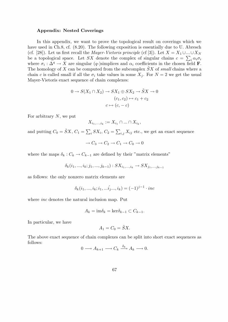
Appendix: Nested Coverings

In this appendix, we want to prove the topological result on coverings which wehave used in Ch.8, cf. (8.20). The following exposition is essentially due to U. Abresch(cf. [28]). Let us first recall the Mayer-Vietoris principle (cf [3]). Let X = X1∪ ...∪XN

be a topological space. Let SX denote the complex of singular chains c =∑

i αiσiwhere σi : ∆q → X are singular (q-)simplices and αi coefficients in the chosen field F.The homology of X can be computed from the subcomplex SX of small chains where achain c is called small if all the σi take values in some Xj. For N = 2 we get the usualMayer-Vietoris exact sequence of chain complexes:

0 → S(X1 ∩X2) → SX1 ⊕ SX2 → SX → 0

(c1, c2) 7→ c1 + c2

c 7→ (c,− c)

For arbitrary N , we put

Xi1,...,ik := Xi1 ∩ ... ∩Xik ,

and putting C0 = SX, C1 =∑

i SXi, C2 =∑

i,j Xij etc., we get an exact sequence

→ C3 → C2 → C1 → C0 → 0

where the maps δk : Ck → Ck−1 are defined by their ”matrix elements”

δk(i1, ..., ik; j1, ..., jk−1) : SXi1,...,ik → SXj1,...,jk−1

as follows: the only nonzero matrix elements are

δk(i1, ..., ik; i1, ...ij..., ik) = (−1)j−1 · inc

where inc denotes the natural inclusion map. Put

Ak = imδk = kerδk−1 ⊂ Ck−1.

In particular, we have

A1 = C0 = SX.

The above exact sequence of chain complexes can be split into short exact sequences asfollows:

0 −→ Ak+1 −→ Ckδk−→ Ak −→ 0.

67

As usual, a short exact sequence of chain complexes gives rise to a long exact sequenceof the homologies:

→ HpAk+1 → HpCk → HpAk → Hp−1Ak+1 → ...

We will use only the segment

HpCk → HpAk → Hp−1Ak+1

in order to estimate the middle term. If we had only to compute the Betti numbers, wewould get

dimHpAk ≤ dimHpCk + dimHp−1Ak+1 (A1)

for all k, and in particular

bp(X) = dimHpA1 ≤ dimHpC1 + dimHp−1A2,

and furtherdimHp−1A2 ≤ dimHp−1C2 + dimHp−2A3

and so on, hence by induction

bp(X) ≤ dimHpC1 + dimHp−1C1 + ...+ dimH0Cp+1

since Hp−qAq+1 = 0 for q > p. However, these Betti numbers are not available in ourapplication; instead, we have to compute the content which is the rank of certain inclu-sion maps. Unfortunately, the analogue of (A1) for the rank in place of the dimensionis not true: If we have a commutative diagram of exact sequences,

Aφ−→B

ψ−→ C

↓ α ↓ β ↓ γ

A′ φ′

−→B′ ψ′

−→ C ′

we have not rk(β) ≤ rk(α) + rk(γ); e.g. we could choose α = 0 and γ = 0, and β mapsim(φ) onto 0 while a complement of imφ is mapped into ker(ψ′). However, if we havethree such sequences,

Aφ−→B

ψ−→ C

↓ α ↓ β ↓ γ

A′ φ′

−→B′ ψ′

−→ C ′

↓ α′ ↓ β′ ↓ γ′

A′′ φ′′

−→B′′ ψ′′

−→ C ′′

68

then we getrk(β′ ◦ β) ≤ rk(α′) + rk(γ).

Proof. Consider a decomposition

im(β) = (imβ)1 ⊕ (imβ)2

where(imβ)1 = im(β) ∩ ker(ψ′).

Then (imβ)1 ⊂ im(φ′), hence

β′(imβ)1 ⊂ φ′′(α′(A′)).

Moreover, ψ′ is injective on (imβ)2, and

ψ′(imβ)2 ⊂ γ(ψ(B)).

Therefore,rk(β′ ◦ β) ≤ dim(β′(imβ)1) + dim(β′(imβ)2)

≤ rk(α′) + rk(γ)

We apply this to

HpC0k −→HpA

0k −→ Hp−1A

0k+1

↓ ↓ ↓HpC

pk −→HpA

pk −→ Hp−1A

pk+1

↓ ↓ ↓HpC

p+1k −→HpA

p+1k −→ Hp−1A

p+1k+1

where Cpk and Apk are the above defined complexes, but now for p+2 different coverings{Xq

1 , ..., XqN} of X (q = 1, ..., p+ 2) with the property that

Xq−1i ⊂ Xq

i

for q = 1, ..., p+ 1 (nested coverings). Thus we get

rk(HpA0k → HpA

p+1k )

≤ rk(HpCpk → HpC

p+1k ) + rk(Hp−1A

0k+1 → Hp−1A

pk+1)

69

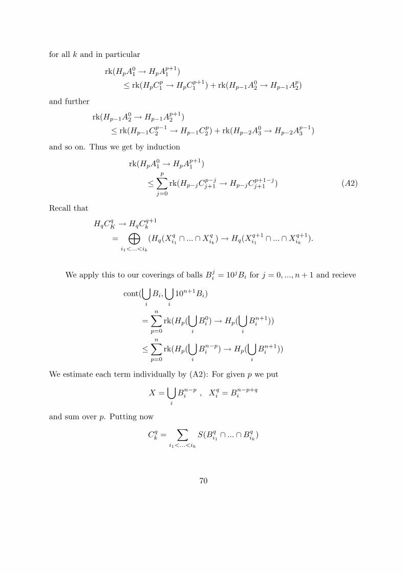
for all k and in particular

rk(HpA01 → HpA

p+11 )

≤ rk(HpCp1 → HpC

p+11 ) + rk(Hp−1A

02 → Hp−1A

p2)

and further

rk(Hp−1A02 → Hp−1A

p+12 )

≤ rk(Hp−1Cp−12 → Hp−1C

p2 ) + rk(Hp−2A

03 → Hp−2A

p−13 )

and so on. Thus we get by induction

rk(HpA01 → HpA

p+11 )

≤p

∑

j=0

rk(Hp−jCp−jj+1 → Hp−jC

p+1−jj+1 ) (A2)

Recall that

HqCqK → HqC

q+1k

=⊕

i1<...<ik

(Hq(Xqi1∩ ... ∩Xq

ik) → Hq(X

q+1i1

∩ ... ∩Xq+1ik

).

We apply this to our coverings of balls Bji = 10jBi for j = 0, ..., n+ 1 and recieve

cont(⋃

i

Bi,⋃

i

10n+1Bi)

=n

∑

p=0

rk(Hp(⋃

i

B0i ) → Hp(

⋃

i

Bn+1i ))

≤n

∑

p=0

rk(Hp(⋃

i

Bn−pi ) → Hp(⋃

i

Bn+1i ))

We estimate each term individually by (A2): For given p we put

X =⋃

i

Bn−pi , Xqi = Bn−p+qi

and sum over p. Putting now

Cqk =∑

i1<...<ik

S(Bqi1 ∩ ... ∩Bqik

)

70

and

γqp,k : HpCqk → HpC

q+1k ,

we get from (A2)

cont(⋃

i

Bi,⋃

i

10n+1Bi)

≤ rk γnn,1 + rk γn−1n−1,2 + ... + rk γ1

1,n + rk γ00,n+1

+ rk γnn−1,1 + rk γn−1n−2,2 + ... + rk γ1

0,n

+ ...+ rk γn1,1 + rk γn−1

0,2

+ rk γn0,1≤ rk γn∗,1 + rk γn−1

∗,2 + ... + rk γ1∗,n + rk γ0

∗,n+1

Hencecont(

⋃

i

Bi,⋃

i

10n+1Bi)

≤n+1∑

k=1

rk γn+1−k∗,k

=

n+1∑

k=1

∑

i1<...<ik

cont(

k⋂

j=1

Bn+1−kij

,

k⋂

j=1

Bn+2−kij

)

which proves Equation (8.20).

References:

[1] Abresch, U. Lower curvature bounds, Toponogov’s theorem and bounded topologyI,II. Ann. scient. Ec. Norm. Sup., 4e serie, t.18 (1985), 651-670

[2] Berger, M.: Les varietes riemanniennes (1/4)-pincees. Ann. Sc. Norm. Super.Pisa, III 14 (1960), 161-170

[3] Bott, R., Tu, L.W.: Differential forms in algebraic topology. Springer GraduateTexts in Mathematics 82 (1982)

[4] Calabi, E.: An extension of E.Hopf’s maximum principle with an application toRiemannian geometry. Duke Math. J. 25 (1957), 45-56

71

[5] Cheeger, J., Ebin, D.G.: Comparison theorems in Riemannian geometry AmericanElsevier, New York 1975

[6] Cheeger, J., Gromoll, D.: On the structure of complete manifolds of nonnegativecurvature. Ann. of Math. 96 (1972), 413-442

[7] Cheeger, J., Gromoll, D.: The splitting theorem for manifolds of nonnegative Riccicurvature. J. Diff. Geom. 6 (1971), 119-128

[8] Cheng, S.Y.: Eigenvalue comparison theorem and its geometric application. Math.Z. 143 (1975), 289-297

[9] Eschenburg, J.-H. Comparison theorems and hypersurfaces. Manuscripta math., 59(1987), 295-323

[10] Eschenburg, J.-H. Diameter, volume, and topology for positive Ricci curvature.Journal of Differential Geometry, 33 (1991), 743-747

[11] Eschenburg, J.-H. Local convexity and nonnegative curvature - Gromov’s proof ofthe sphere theorem. Invent. math., 84 (1986), 507-522

[12] Eschenburg, J.-H. Maximum Principle for Hypersurfaces, Manuscripta Math. 64(1989), 55 - 75

[13] Eschenburg, J.-H., Heintze, E. An elementary proof of the Cheeger - Gromoll split-ting theorem. Ann. Glob. Analysis and Geometry, vol. 2, n. 2 (1984), 141-151

[14] Eschenburg, J.-H., Heintze, E. Comparison theory for Riccati equation Manuscriptamath., 68 (1990), 209-214

[15] Green, L.W.: A theorem of E.Hopf. Mich. Math. J. 5 (1958), 31-34

[16] Greene, R.E., Wu, H.: On the subharmonicity and plurisubharmonicity of geodesi-cally convex functions. Ind. Univ. Math. J. 22 (1973), 641-653

[17] Greene, R.E., Wu, H.: C∞-convex functions and manifolds of positive curvature.Acta Math. 137 (1976), 209-245

[18] Gromoll, D., Klingenberg, W., Meyer, W.: Riemannsche Geometrie im GroßenLecture notes 55, Springer 1968

72

[19] Gromov, M.: Curvature, diameter and Betti numbers. Comm. Math. Helv. 56(1981), 179-195

[20] Gromov, M.: Structures metriques pour les varietes riemanniennes. Cedic-Nathan1981

[21] Grove, K., Shiohama, A.: A generalized sphere theorem. Ann. of Math. 106 (1977),201-211

[22] Hadamard, J.: Sur certain proprietes des trajectories en dynamique. J. Math.Pures Appl. (5)3 (1897), 331-387

[23] Hopf, E.: Elementare Bemerkungen uber die Losungen partieller Differentialgle-ichungen 2.Ordnung vom elliptischen Typ. Sitzungsber. Preuss. Ak. d. Wiss. 19(1927), 147-152

[24] Karcher, H.: Riemannian comparison constructions. In: S.S.Chern (ed.): Studiesin Global Geometry and Analysis, M.A.A. Studies in Mathematics, vol. 27 (1989)

[25] Klingenberg, W.: Uber Riemannsche Mannigfaltigkeiten mit positiver Krummung.Comm. Math. Helv. 35 (1961), 47-54

[26] Kobayashi, S., Nomizu, K.: Foundations of differential geometry, I. Interscience,Wiley, New York 1963

[27] Kurzel, M. Der Vergleichssatz von Toponogov im Fall variabler Krummung. Diplo-marbeit, Munster 1994

[28] Meyer, W. Toponogov’s theorem and applications. Preprint University of Munster(1990)

[29] Milnor, J.: Morse Theory. Princeton 1962

[30] Milnor, J.: A note on curvature and fundamental group. J. Diff. Geom. 2 (1968),1-7

[31] Myers, S.B.: Riemannian manifolds with positive mean curvature. Duke Math. J.8 (1941), 401-404

[32] Sharafutdinov, V.A.: Convex sets in a manifold of nonnegative curvature. Math.

73

Zametki 26 (1979) 556-560

[33] Strake, M., Walshap, G. : Σ-flat manifolds and Riemannian submersions. Manuscr.Math. 64 (1989), 213-226

[34] Wu, H.: An elementary method in the study of nonnegative curvature. Acta Math.142 (1979), 57-78

[35] J.-W.Yim: Distance nonincreasing retraction on a complete open manifold of non-negative sectional curvature. Ann. Glob. Anal. and Geom.

74

Contents

0. Introduction. 11. Covariant derivative and curvature. 22. Jacobi and Riccati equations; equidistant hypersurfaces. 63. Comparison theory. 124. Average comparison theoremx. 155. Bishop-Gromov inequality 176. Toponogov’s triangle comparison theorem 217. Number of generators and growth of the fundamental group 268. Gromov’s estimate of the Betti numbers 319. Convexity 3910. Open manifolds with nonnegative curvature 4311. The sphere theorem 5012. Lower Ricci curvature bounds and the Maximum Principle. 5913. The Bochner technique. 65Appendix: Nested coverings 67References 72Contents 75Index 76

75

Index

affine function 63Betti numbers 30Bishop-Gromov inequality 17,20Busemann function 43,44,62Bochner 65comparison theorem 12complete 5compressible 33concave 39,44conjugate points 18content 32convex 39,43,52convex hypersurface 40corank 34critical points 31,33,34curvature tensor 3cut locus 17diameter 26distance 2,9divergence 63end 64equidistant hypersurfaces 9,13exponential coordinates 5exponential map 5,18focal points 9free action 26fundamental group 26,59,64fundamental domain 26Gauss map 52geodesic 4gradient 2gradientlike 30growth of a group 28,29Hopf-Calabi maximum principle 60Hopf-Rinow theorem 17,19Hadamard 52horospheres 43incompressible 34

76

in the sense of support functions 39,60Jacobi field 6Killing field 66k(p,r) 34Laplacian 60length 2Levi-Civita derivative 2line 59local gradient 8,65Mayer-Vietoris principle 67mean curvature 9,15Morse theory 30,34normal bundle 43open manifold 43parallel 4,12,63Perelman’s theorem 47principal curvatures 9,13ray 43regular point 31Riccati equation 8,12Riemannian manifold 2Riemannian product 59Ricci curvature 3rigidity theorem 60scalar curvature 3sectional curvature 3shape operator 9Sharafutdinov 47,49shortest curve 2,17soul 43sphere theorem 50standard space 19subharmonic 60superharmonic 60support function 25,39Toponogov theorem 22totally geodesic 14umbilical 10vector field along a map 4

77