GW100: Benchmarking G0W0 for molecular systems

Michiel J. van Setten,∗,†,‡ Fabio Caruso,¶,§ Sahar Sharifzadeh,‖ Xinguo Ren,#,@

Matthias Scheffler,@ Fang Liu,4 Johannes Lischner,∇, Lin Lin, Jack R. Deslippe,

Steven G. Louie,,∇ Chao Yang, Florian Weigend,, Jeffey B. Neaton, Ferdinand

Evers, and Patrick Rinke,@

Nanoscopic Physics, Institute of Condensed Matter and Nanosciences, Université

Catholique de Louvain, Louvain-la-Neuve, 1348, Belgium, Institute of Nanotechnology,

Karlsruhe Institute of Technology Campus North, Karlsruhe, 76344 Germany,

Fritz-Haber-Institut der Max-Planck-Gesellschaft, Berlin, 4195, Germany, Department of

Materials, University of Oxford, Oxford, OX1 3PH, United Kingdom, Molecular Foundry,

Lawrence Berkeley National Laboratory, Berkeley, CA 94720, USA, Department of

Electrical and Computer Engineering, Boston University, Boston, MA 02215, USA, Key

Laboratory of Quantum Information, University of Science and Technology of China, Hefei,

230026, China, Fritz-Haber-Institut der Max-Planck-Gesellschaft, Berlin, 14195, Germany,

School of Applied Mathematics, Central University of Finance and Economics, Beijing,

Materials Sciences Division, Lawrence Berkeley National Laboratory, Berkeley, CA 94720,

USA, Department of Physics, University of California, Berkeley, CA 94720, USA,

Computational Research Division, Lawrence Berkeley National Laboratory, Berkeley, CA

94720, USA, National Energy Research Scientific Computing Center, Berkeley, CA 94720,

USA, Department of Physics, University of California, Berkeley, CA 94720, USA ,

Institute of Nanotechnology, Karlsruhe Institute of Technology Campus North, Karlsruhe,

76344, Germany, Institute of Theoretical Physics, University of Regensburg, Regensburg,

93040, Germany, and COMP/Department of Applied Physics, Aalto University School of

Science, Aalto, 00076, Finland

E-mail: michiel.vansetten@uclouvain.be

2

May 16, 2015

Abstract

ab initio GW calculations for 100 molecules, a benchmark set we term as GW100,

are presented using three independent codes and using different methods. Quasiparticle

highest-occupied molecular orbital (HOMO) and lowest-unoccupied molecular orbital

(LUMO) energies are calculated for the GW100 set at the G0W0@PBE level using

the software packages TURBOMOLE, FHI-aims, and BerkeleyGW . The use of these

three codes allows for a quantitative comparison of the type of basis set (plane wave

or local orbital) and handling of unoccupied states; the treatment of core and valence

electrons (all electron or pseudopotentials); the treatment of the frequency dependence

of the self-energy (full frequency or more approximate plasmon-pole models); and the

algorithm for solving the quasiparticle equation. A primary result are reference values

for future benchmarks, best practices for convergence within a particular approach, and

average error-bars for the most common approximations.

∗To whom correspondence should be addressed†Nanoscopic Physics, Institute of Condensed Matter and Nanosciences, Université Catholique de Louvain,

Louvain-la-Neuve, 1348, Belgium‡Institute of Nanotechnology, Karlsruhe Institute of Technology Campus North, Karlsruhe, 76344 Ger-

many¶Fritz-Haber-Institut der Max-Planck-Gesellschaft, Berlin, 4195, Germany§Department of Materials, University of Oxford, Oxford, OX1 3PH, United Kingdom‖Molecular Foundry, Lawrence Berkeley National Laboratory, Berkeley, CA 94720, USA⊥Department of Electrical and Computer Engineering, Boston University, Boston, MA 02215, USA#Key Laboratory of Quantum Information, University of Science and Technology of China, Hefei, 230026,

China@Fritz-Haber-Institut der Max-Planck-Gesellschaft, Berlin, 14195, Germany4School of Applied Mathematics, Central University of Finance and Economics, Beijing∇Materials Sciences Division, Lawrence Berkeley National Laboratory, Berkeley, CA 94720, USADepartment of Physics, University of California, Berkeley, CA 94720, USAComputational Research Division, Lawrence Berkeley National Laboratory, Berkeley, CA 94720, USANational Energy Research Scientific Computing Center, Berkeley, CA 94720, USADepartment of Physics, University of California, Berkeley, CA 94720, USAInstitute of Nanotechnology, Karlsruhe Institute of Technology Campus North, Karlsruhe, 76344, Ger-

manyInstitute of Theoretical Physics, University of Regensburg, Regensburg, 93040, GermanyCOMP/Department of Applied Physics, Aalto University School of Science, Aalto, 00076, FinlandInstitute of Physical Chemistry, Karlsruhe Institute of Technology Campus South, Karlsruhe, 76021,

Germany

3

1 Introduction

Computational spectroscopy is developing into a complementary approach to experimen-

tal spectroscopy. It facilitates the interpretation of experimental spectra and can predict

properties of hitherto unexplored materials. In computational spectroscopy as in any other

theoretical discipline the first step is the definition of the physical model. In theoretical

physics and chemistry, this model is governed by a set of equations. Computational sciences

solve these equations numerically and the solutions should of course be independent from

the computational settings. However, in reality this is not always the case. In practice, the

equations are often complicated and the numerical techniques introduce many, often inter-

dependent, computational parameters. A thorough validation of these parameters can be

very time consuming.

To validate computational approaches, theoretical benchmarks are essential. In quan-

tum chemistry, benchmark sets are well established (e.g. G2/97,1–3 GMTKN30,4 ISO34,5,6

S667). In solid state physics, a validation benchmark set for elementary solids has only

recently been published for ground state properties calculated in density-functional theory

(DFT).8 According to Refs. 8,9 several DFT codes differ by a surprising amount even for

the computationally efficient semi-local Perdew-Burke-Ernzerhof (PBE) functional.10

The physical model we address in this article describes charged electronic excitations and

we here apply it to molecules. We focus on Hedin’s GW approximation11 where G is the

single particle Green’s function and W the screened Coulomb interaction. For solids GW

has become the method of choice for the calculation of quasiparticle spectra as measured

in direct and inverse photoemission.12–14 Recently, the GW approach has also increasingly

been applied to molecules and nano-structures.15–51

In its simplest form (G0W0), the GW approach is applied as correction to the electronic

spectrum of a non-interacting reference Hamiltonian, such as Kohn-Sham DFT or Hartree-

Fock11–14 (in the following denoted @reference). However, despite G0W0’s more than 50 year

history and, starting 30 years ago, its practical implementation within electronic structure

4

framework,52–54 results from different codes and approximations have rarely been directly

compared. In this article, we provide a thorough assessment of G0W0, with a particular

starting point, for gas-phase molecules using three different codes, validating different com-

putational implementations and elucidating best practices for convergence parameters, such

as basis sets, treatment of the unoccupied subspace, and discretization meshes.

In this work, we make the first step and establish a consistent set of benchmarks of

ionization energies and electron affinities of 100 molecules – the GW100 set. We present

converged G0W0 calculations based on the Perdew-Burke-Ernzerhof (PBE)10 generalized

gradient approximation to DFT. Our G0W0@PBE results for these molecules can serve as

reference for future G0W0 implementations and calculations. We apply three different G0W0

codes in this work: TURBOMOLE,48 FHI-aims,39,55 and BerkeleyGW.56 The three codes

differ in their choice of basis set (atom centered orbitals in TURBOMOLE and FHI-aims

and plane waves in BerkeleyGW), and in their implementation. The validation process was

crucial to remove conceptual and numerical inconsistencies from our implementations and

to test the influence of all computational settings. In the end, all three codes agree to within

0.1 eV for ionization energies and electron affinities. TURBOMOLE and FHI-aims are all-

electron codes and use the same basis sets in this work.1 They agree to∼1 meV. BerkeleyGW,

employing a real-axis full-frequency method and pseudopotentials, leads to results that differ

from TURBOMOLE and FHI-aims by 100 meV on average. We consider this residual

discrepancy as acceptable for the time being, since where FHI-AIMS and TURBOMOLE

use the same (local-orbital) basis set and BGW uses a plane wave basis set, which makes

it applicable also to extended systems. Whether or not there is another dominating source

remains to be investigated.

In the GW100 set, we also supply experimental ionization energies and electron affinities,

where available. These are intended for future reference. An assessment of the GW method

as such is beyond the scope of this work and would require an extensive study of the starting-1The calculations perfomed in this work are all explicitly non-relitivistic to exclude effects of different

relativistic approaches.

5

point dependence of G0W0.14,38,41,42,46,50,57,58 Moreover, when trying to validate by direct

comparison to experiment, care has to be taken, because experimental data tends to carry

uncertainties that are intrinsic to the measuring process or reflect external influences (e.g.,

defects or disorder) and other environmental parameters (e.g., temperature). These effects

are not included in our theoretical approach here.

The remainder of the article is structured as follows: We start by describing the test set

that will be used in this paper in Sec. 2. In Sec. 3 we present the G0W0 approaches used in

this work and explain their similarities and differences. In Sec. 4 the ionization energies and

electron affinities of the GW100 are presented. In Sec. 5 we discuss the different ways to

treat the analytic structure of W in our three G0W0 approaches. In Sec. ?? we quantify the

effects of the different approximations on the quasi-particle energies. The main conclusions

are summarized in Sec. 6.

2 The GW 100 set

The 100 molecules in the GW100 set includes different elements and thereby covers a con-

siderable range of ionization potentials (from ca. 4 eV for Rb2 to ca. 25 eV for He). The

selected molecules exhibit a spectrum of typical chemical bonding situations. For instance,

for carbon we include a variety of covalent bonds, such as C2H6, C2H4, C2H2, C6H6, CO,

CO2 and C4. Special interest is devoted to bonds of metal atoms by including Cu2 and Ag2,

Li2, K2, Na2, and Rb2 as well as small metallic clusters Na4 and Na6. In contrast, alkaline

metal halides are prototypes for ionic bonds, LiF being an extreme and KBr a more moderate

case. The alkaline earth metal compounds MgF2 and MgO are also ionic, the former with

a vanishing, the latter with a large dipole moment. Including series of homologous like N2-

P2-As2, F2-Cl2-Br2-I2 or CF4, CCl4, CBr4, CI4 facilitates the identification of trends within

a group of elements. These trends can then be correlated with certain physical or chemical

properties, such as the decreasing ionic bond character in the last example. Furthermore, we

6

have also included several simple organic molecules, like alcohols, aldehydes and nitrogenous

bases, as well as the most typical test cases often appearing in benchmark sets such as water,

and carbon mono- and dioxide.

The molecular geometries used in this work are mainly taken from experiment. For some

molecules the final structure was obtained by optimizing a known morphology using DFT in

the PBE approximation for the exchange-correlation functional using the def2-QZVP basis

set. All molecular geometries are included in the supporting material.

3 Computational Methodology

The objective of this work is to establish a set of converged and validated G0W0 results for

molecules that will serve as a benchmark for future work. Specifically, we calculate the G0W0

self-energy11

Σσ(r, r′, ω) =i

2π

∫ +∞

−∞dω′Gσ

0 (r, r′, ω + ω′)W0(r, r′, ω′), (1)

where Gσ0 denotes the one-particle causal Green’s function for spin channel σ =↑, ↓ andW0 is

the screened Coulomb interaction in the random-phase approximation (RPA). Traditionally,

one splits the self-energy into energy dependent correlation and energy independent exchange

terms as

Σσ(ω) = Σσx + Σσ

c (ω). (2)

Gσ0 is given in terms of the single-particle wave functions ψKS

nσ (r) and eigenvalues εKSnσ of

a reference Kohn-Sham DFT calculation2

Gσ0 (r, r′, ω) =

∑n

ψKSnσ (r)ψKS∗

nσ (r′)

ω − εKSnσ − iη sgn(εF − εKS

nσ ), (3)

2In this paper we only consider DFT Kohn-Sham reference Hamiltonians. In general, other single-particleHamiltonians such as Hartree or Hartree-Fock are also permissible.

7

where εF is the Fermi level (chemical potential) and η a positive infinitesimal. W0 follows

from the non-interacting response function χ0 that in a real-space representation assumes

the following form

χ0(r, r′, ω) = − i

2π

∫ +∞

−∞dω′ Gσ

0 (r, r′, ω + ω′) Gσ0 (r′, r, ω′), (4)

=∑σ

∑n,m

(fn − fm)ψKS∗nσ (r)ψKS

mσ(r)ψKS∗mσ (r′)ψKS

nσ (r)

ω − εKSmσ + εKS

nσ + iη, (5)

where the second line is the sum-over states representation of Adler and Wiser59,60 and

fm, fn are the occupation factors of states m and n, respectively. Given the non-interacting

response function χ0, W0 is expanded in powers of χ0

W0 = v + vχ0v + vχ0vχ0v + · · · = v + vχv, (6)

where we have omitted the space and frequency variables for simplicity. The last equal sign

in Eq. 6 introduces the reducible response function χ = χ0[1− vχ0]−1.

Given the G0W0 self-energy, the quasi-particle (QP) energies εQPn are computed by solving

the diagonal QP-equation in the basis of the single-particle states |nσ〉, i.e.

εQPnσ = εKS

nσ + 〈nσ|Σσ(εQPnσ )− vxc|nσ〉 . (7)

In the above equation vxc denotes the exchange-correlation potential of the preceding DFT

calculation.

In our comparative study we use a DFT-PBE starting point. Once we have decided on

this reference Hamiltonian, G0 is uniquely defined. As a result, Σ in the G0W0 approximation

is also uniquely defined and all G0W0 implementations should, in principle, produce the same

G0W0@PBE results. However, G0W0 implementations can differ in several aspects, that in

practice can lead to deviations. The most critical aspects are listed as follows.

8

a) The choice of the basis set: In this work we will compare GW results obtained

with both local orbital (LO) and plane wave (PW) basis sets. In a local basis set, the

size of the Hamiltonian is usually significantly smaller than in plane waves: for example for

ethene, with the LO basis used here, about 350 functions were used; the analogous plane

wave calculation used a factor of 225 more functions. However, for an LO basis there is

no unique recipe to systematically increase the basis set to approach the complete basis

set limit. Conversely, a plane wave basis set is conceptually easier to converge: one main

parameter, the kinetic energy cutoff, needs to be increased until convergence is achieved.

However, plane waves require periodic boundary conditions, and molecules therefore have to

be placed in a supercell, a large, periodically repeated box that is filled with vacuum. While

the size of the supercell usually convergences quickly for local and semi local DFT functionals,

the screened Coulomb W0 interaction in G0W0 can be long-ranged. A brute force supercell

convergence is therefore computationally impractical.61 Instead, the Coulomb interaction

is truncated,62,63 which introduces, in principle, an additional convergence parameter. In

BerkeleyGW, this truncation is automatically based on supercell size. To compute ionization

energies and electron affinities, we correct for the shift in vacuum level that is present due

to periodic boundary conditions. Taking the molecule at the center of the supercell, the

vacuum correction is calculated as the electrostatic potential at the supercell edges.

In plane wave G0W0 calculations, additional energy cutoffs are often introduced that

reduce the number of unoccupied states included in the empty state summations of the

Green’s function (Eqn. 3) and the non-interacting response function (Eqn. 5).64–66 These

energy cutoffs can reduce the computational cost, albeit at the expense of new convergence

parameters. On the other hand, the use of a small number of basis functions in local orbital

calculations can limit the number and the accuracy of empty states above the vacuum level.

If in this situation a systematic extrapolation to the basis set limit is not feasible this can

lead to limitations in the accuracy of the response function given by Eq. 5, and G0 and W0,

and therefore the self energy itself.

9

G0W0 has also been implemented in other basis sets, such as projector augmented waves

(PAW), see e.g. Refs. 67, 64 and 68, and linear augmented plane waves (LAPW), see e.g.

Refs. 69, 70, 71 and 72, and linearized muffin tin orbitals (LMTO), see e.g. Ref. 73. These

implementations have not been included in the present test.

b) The treatment of core electrons and valence electrons in the core regions:

In the FHI-aims and TURBOMOLE calculations in this work we included all electrons

explicitly at each step of the calculation. However, at the moment a pure plane wave basis set

requires pseudopotentials that remove the rapid oscillations of the electronic wave functions

near the nuclei and hence drastically reduce the required energy cutoff. In a pseudopotential

approach, the electrons are divided into core and valence electrons. The core electrons are

frozen in their atomic ground state and are used to generate a smooth potential for the

valence electrons.74–79 On the DFT level, pseudopotentials are typically derived from single-

atom DFT calculations performed with the same functional as used later.

However, interactions between core and valence electrons that depend on the environ-

ment in a polyatomic system undermine the transferability and lead to deviations between

pseudopotential and all-electron calculations. The use of pseudopotentials can lead to er-

rors in GW calculations because of the neglect of core polarization effects;14,80 deviations in

the pseudo and all-electron wave functions near the nucleus;81,82 and core-valence interac-

tions.81,82 To shed more light on the quantitative role of core electrons and pseudopotentials,

we directly compare all-electron, frozen core, and pseudopotential G0W0 calculations in this

work.

DFT-PBE pseudopotentials are used in our planewave G0W0 calculations. All valence

electrons of the same principal quantum number are treated on the G0W0 level, whereas the

description of the core electrons and the core-valence interaction remains on the DFT level.

c) Treatment of the frequency dependence: All quantities in G0W0 depend explicitly

on a frequency (or time) argument (see Sec. 3). Different G0W0 implementations differ

10

in their treatment of this frequency dependence. Since the poles in G0 and all subsequent

quantities lie close to the real frequency axis, all quantities in G0W0 exhibit a pronounced fine

structure on the real frequency axis, whose resolution requires fine frequency grids and a large

number of frequency points. Different strategies are employed to avoid the computational

bottleneck of dense frequency grids. In this work we will compare several different ways: the

fully analytic treatment in TURBOMOLE (TM-RI) and (TM-noRi),? an integration on

the imaginary axis with subsequent analytic continuation to the real axis as implemented in

FHI-aims (AIMS-2P) and (AIMS-P16),39,55 and the BerkeleyGW implementation of the full

frequency treatment on the real axis (BGW-FF)83 and of a generalized plasmon pole model

(BGW-GPP).53 Techniques employing contour deformation and approaches to circumvent

the sum over empty states have also been reported in the literature,84–87 but they are not

considered in this work.

d) Solution of the QP-equation: The final step in G0W0 is the calculation of the QP-

energies by solving Eq. 7. A technical aspect that we draw particular attention to is the

occurrence of multiple solutions in the QP-equation.88–90 Since not all GW codes search for

all solutions, differentG0W0 implementations may give different answers for multiple-solution

cases although the underlying self-energies may be very similar.

Summarizing, the impact of these differing approaches a)-d) can affect the QP-energies

in a significant way, which has only in part been quantified by previous studies.39,44,48,81,82

Apart from code validation, a second main goal of our work is a quantitative comparison of

different methods. This goal will be achieved by comparing the G0W0 results (i.e., the QP-

energies) obtained from three different G0W0 implementations TURBOMOLE, FHI-aims,

and BerkeleyGW.

In the following sections we describe the conceptual and technical differences that dis-

tinguish the TURBOMOLE, FHI-aims, and BerkeleyGW G0W0 implementations. A more

general description of the GW method and its application to molecules in particular can be

11

found in various reviews12–14,48,91,92 and is not the topic of this paper. We will also provide

detailed convergence studies of the relevant computational parameters.

3.1 The frequency dependence of the G0W0 self-energy

A pronounced difference between different G0W0 implementations is the treatment of the

frequency dependence of the self-energy in Eq. (1) and of intermediate quantities. In this

work we will compare an analytic treatment of the pole structure facilitated by the spectral

representation of the response function with a plasmon-pole model and a numerical real as

well as imaginary frequency treatment. In the next four sections we describe the technical

aspects of these approaches. The implications on the results of these different approaches

will be discussed in the results and discussion sections.

3.1.1 Implementation of the fully analytic (FA) spectral representation in TUR-

BOMOLE

The RPA response function (Eq. 5 and 6) is calculated explicitly in its spectral representation.

Since the Green’s function G0 has Nocc +Nunocc poles, the screened interaction W0 exhibits

2×NoccNunocc poles. As the exact pole positions of W0 are inherited from G0 and therefore

known, we can evaluate the energy integral for Σ (Eq. 1) analytically. This gives Σ 2 ×

(Nocc +Nunocc)NoccNunocc poles. In the rest of this section we summarize the most important

technical details following Ref. 48 where we here focus on the non-magnetic case: ψ = ψ↑ =

ψ↓.

The implementation of G0W0 in TURBOMOLE is based on the spectral representation

of the reducible response function.

χ(r, r′, ω) =∑m

ρm(r)ρm(r′)

(1

ω + iη − Ωm

− 1

ω − iη + Ωm

). (8)

The pole positions, Ωm, are the (charge neutral) excitation energies and the ρm(r) denote

12

transition densities. The ρm are be expanded in a basis of orbital products,

ρm(r) =∑i,a

(Xm + Ym)i,a ψi(r)ψa(r), (9)

where i, j, .. label occupied states and a, b, .. label empty states. The vectors |Xm, Ym〉 are

solutions of the eigenvalue problem

(Λ− Ωm∆) |Xm, Ym〉 = 0 (10)

under the orthonormality constraint

〈Xm, Ym|∆ |Xm′ , Ym′〉 = δm,m′ . (11)

The operators

Λ =

A B

B A

, ∆ =

1 0

0 −1

(12)

contain the orbital rotation Hessians:

(A + B)iajb = (εa − εi)δijδab + 2 〈ij|ab〉 (13)

(A− B)iajb = (εa − εi)δijδab (14)

with 〈ij|ab〉 =∫drdr′ψi(r)ψj(r

′) 1|r−r′|ψa(r)ψb(r

′).

From the reducible response function the screened Coulomb interactionW can be directly

constructed by contracting with Coulomb interaction v:

W (ω) = v + v · χ(ω) · v (15)

The self-energy can finally be obtained directly by performing the energy integral ana-

lytically since in this formalism the energy structure of both G and W is known. Performing

13

the integral leads to a closed expression for the matrix elements of the self-energy. The real

part of the diagonal matrix elements of Σ includes the exchange contribution

〈n|Σx |n〉 = −∑i

(ni|in) (16)

while for the correlation contribution we have

< (〈n|Σc(εn) |n〉) =1

2

∑m

[∑i

|(in|ρm)|2 εn − εi + Ωm

(εn − εi + Ωm)2 + η2+∑a

|(an|ρm)|2 εn − εa − Ωm

(εn − εa − Ωm)2 + η2

],

(17)

where as before m runs over all density excitations and η is an infinitesimal.

3.1.2 BerkeleyGW implementation of the full frequency (FF) integration along

the real frequency axis

The FF-BerkeleyGW approach evaluates the frequency dependent self-energy numerically,

along the real frequency axis. Similar to the TURBOMOLE implementation, G0, W0 and

Σ retain the full pole structure. However, unlike in TURBOMOLE, the pole structure is

represented on the frequency grid.

In FF-BerkeleyGW the frequency dependent self-energy is

Σ(r, r′, ω) =−Nocc∑j=1

ψKSj (r)ψ∗KS

j (r′)v(r, r′)

− 1

2πi

Nocc∑j=1

ψKSj (r)ψ∗KS

j (r′)

∫ ∞0

dω′W r(r, r′, ω′)−W a(r, r′, ω′)

ω − εKSj + ω′ − iη

− 1

2πi

Nocc+Nunocc∑a=Nocc+1

ψKSa (r)ψ∗KS

a (r′)

∫ ∞0

dω′W r(r, r′, ω′)−W a(r, r′, ω′)

ω − εKSa − ω′ + iη

,

(18)

where W r/a are the retarded (r) and advanced (a) screened Coulomb matrix which can be

14

expressed as

W r/a(r, r′, ω) ≡∫

[εr/a(r, r′′, ω)]−1v(r′′, r′)dr′′, (19)

where the retarded/advanced dielectric function εr/a has the form

εr/a(r, r′, , ω) = δ(r, r′)−∫v(r, r′′)χ

r/a0 (r′′, r′, ω)dr′′,

and the retarded/advanced reducible polarizability is defined as

χr/a0 (r, r′, ω) =

1

2

Nocc∑i=1

Nocc+Nunocc∑j=Nocc+1

ψKSi (r)ψ∗KS

j (r)ψ∗KSi (r′)ψKS

j (r′)

×(

1

ω −∆εKSi,j ± iη

− 1

ω + ∆εKSi,j ± iη

),

(20)

where ∆εi,j = εj − εi ≥ 0.

The integral in (18) is evaluated numerically on the interval [0, ωcuthigh], beyond which the

integrand is negligibly small. We further reduce computational cost by dividing the interval

[0, ωcuthigh] into two intervals: [0, ωcutlow] and [ωcutlow, ωcuthigh] treated with two different integration

schemes. The low frequency cutoff ωcutlow is chosen to ensure that all poles of the numer-

ator in the integrand lie below ωcutlow; therefore the integrand decays smoothly beyond this

point. A uniform fine frequency step ∆ω is used on [0, ωcutlow], while a smaller number of

quadrature points can be used to perform a standard numerical integration of Eq. 18 within

the interval [ωcutlow, ωcuthigh]. Because the integrand contains a number of singularities in the

interval [0, ωcutlow], we use the special integration scheme of Ref. 93 to perform the numerical

integration accurately on this interval.

For all of the 18 molecules studied with FF-BGW, we use η = 0.2 eV and ∆ω = 0.2 eV.

We tested the convergence of our calculations with respect to these parameters by varying

both until the results no longer change. Figure 1 shows an example for the ethylene molecule,

with the dependence of the quasiparticle energy on the parameters η and ∆ω for predicted

QP-HOMO energy. Since here our aim is to test the convergence behavior for η and ∆ω,

15

we used a low Ecutε of 5.0 Ry. Figure 1 shows that for a given η, ∆ω = η is sufficient for an

accuracy of 0.01 eV and that η = 0.2 eV is sufficient.

In a plane wave basis the number of basis functions is much larger than in the localized

basis set used in TURBOMOLE and FHI-aims. Therefore, intermediate quantities such as

the dielectric function and the self-energy require larger matrices. To keep the calculation

tractable, the dielectric function is only computed for a reduced set of plane waves, with plane

wave cutoff energy Ecutε . In addition, the number of unoccupied states that enter the Green’s

function and the self-energy is controlled by the energy of the highest unoccupied state, Emax.

Since Ecutε and Emax are interdependent,36 careful convergence studies are required. Here, we

converged these parameters within GPP-GW as will be described below. We converged the

dielectric function by increasing both Emax and Ecutε until the screened exchange component

of the self-energy changed by less than 0.2 eV and extrapolate the Coulomb-hole term of the

self energy by means of static completion method.94 Within this approach, a term is added

to the Coulomb-hole component of Σ which corrects for the truncation of the number of

unoccupied states.94

In Table 1 the values of the parameters introduced in this section are listed for 18

molecules studied with FF-BGW.

−12.02 −12.01 −12 −11.99

−12.02

−12.015

−12.01

−12.005

−12

−11.995

−11.99

−11.985

ω (eV)

EL

DA

−V

XC

+R

e(Σ

(ω))

(e

V)

η=0.2, ∆ω=0.2

η=0.1, ∆ω=0.1

η=0.05, ∆ω=0.05

η=0.2, ∆ω=0.1

η=0.1, ∆ω=0.05

η=0.05, ∆ω=0.025

y=x

−8.7 −8.6 −8.5 −8.4−9.1

−9

−8.9

−8.8

−8.7

−8.6

−8.5

−8.4

−8.3

−8.2

−8.1

ω (eV)

EL

DA

−V

XC

+R

e(Σ

(ω))

(e

V)

η=0.2, ∆ω=0.2

η=0.1, ∆ω=0.1

η=0.05, ∆ω=0.05

η=0.2, ∆ω=0.1

η=0.1, ∆ω=0.05

η=0.05, ∆ω=0.025

y=x

Figure 1: The QP-HOMO of an Ethylene (left) and BeO (right) molecule with different ηand ∆ω.

16

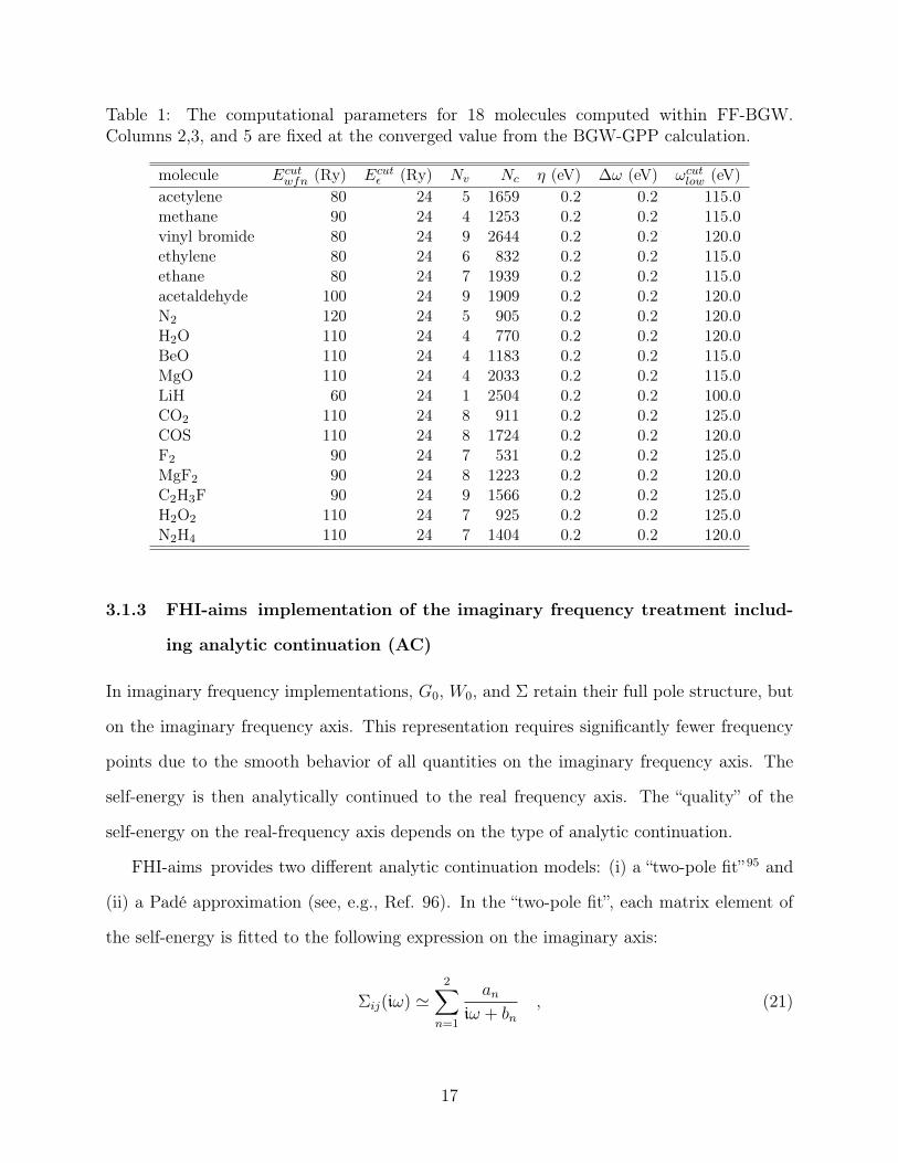
Table 1: The computational parameters for 18 molecules computed within FF-BGW.Columns 2,3, and 5 are fixed at the converged value from the BGW-GPP calculation.

molecule Ecutwfn (Ry) Ecutε (Ry) Nv Nc η (eV) ∆ω (eV) ωcutlow (eV)acetylene 80 24 5 1659 0.2 0.2 115.0methane 90 24 4 1253 0.2 0.2 115.0vinyl bromide 80 24 9 2644 0.2 0.2 120.0ethylene 80 24 6 832 0.2 0.2 115.0ethane 80 24 7 1939 0.2 0.2 115.0acetaldehyde 100 24 9 1909 0.2 0.2 120.0N2 120 24 5 905 0.2 0.2 120.0H2O 110 24 4 770 0.2 0.2 120.0BeO 110 24 4 1183 0.2 0.2 115.0MgO 110 24 4 2033 0.2 0.2 115.0LiH 60 24 1 2504 0.2 0.2 100.0CO2 110 24 8 911 0.2 0.2 125.0COS 110 24 8 1724 0.2 0.2 120.0F2 90 24 7 531 0.2 0.2 125.0MgF2 90 24 8 1223 0.2 0.2 120.0C2H3F 90 24 9 1566 0.2 0.2 125.0H2O2 110 24 7 925 0.2 0.2 125.0N2H4 110 24 7 1404 0.2 0.2 120.0

3.1.3 FHI-aims implementation of the imaginary frequency treatment includ-

ing analytic continuation (AC)

In imaginary frequency implementations, G0, W0, and Σ retain their full pole structure, but

on the imaginary frequency axis. This representation requires significantly fewer frequency

points due to the smooth behavior of all quantities on the imaginary frequency axis. The

self-energy is then analytically continued to the real frequency axis. The “quality” of the

self-energy on the real-frequency axis depends on the type of analytic continuation.

FHI-aims provides two different analytic continuation models: (i) a “two-pole fit” 95 and

(ii) a Padé approximation (see, e.g., Ref. 96). In the “two-pole fit”, each matrix element of

the self-energy is fitted to the following expression on the imaginary axis:

Σij(iω) '2∑

n=1

aniω + bn

, (21)

17

where the dependence of a and b on i and j has been omitted for simplicity. In the Padé

approximation Σij is given by:

Σij(iω) 'a0 + a1(iω) + · · ·+ a(N−1)/2(iω)(N−1)/2

1 + b1(iω) + · · ·+ bN/2(iω)N/2, (22)

where N is the total number of parameters employed in the Padé expansion. The ionization

energies and electron affinities in Tables 2 and 5 have been calculated using N = 16 (which

is equivalent to a sum of 8 poles). Σ on the real-frequency axis is then obtained by replacing

iω with ω in Eq. 21 or 22 and the G0W0 quasi-particle energies are obtained by solving Eq. 7.

3.1.4 Generalized Plasmon Pole (GPP) in the BerkeleyGW implementation

Within our GPP implementation,56 the expression for the self-energy, Σ, is written as the

sum of two terms, termed the screened-exchange (SX) and coulomb-hole (CH). Here,

ΣSX(ω) =Nv∑j=1

(ψKSj ψ∗KS

j

)× Ω2 (1− i tan Φ)

(ω − εj)2 − ω2V (23)

and

ΣCH(ω) =1

2

∑n′′

(ψKSn′′ ψ∗KS

n′′

)× Ω2 (1− i tan Φ)

ω (ω− εn′′− ω)V (24)

where j runs over occupied states, n′′ run over both occupied and unoccupied states, and Ω,

ω, λ and Φ are, respectively, the effective bare plasma frequency, the GPP mode frequency,

the amplitude, and the phase of the renormalized Ω2, defined in reciprocal space as:

Ω2GG′(q) = ω2

p

(q+G)·(q+G′)

|q+G|2ρ(G−G′)ρ(0)

(25)

ω2GG′(q) =

|λGG′(q)|cos ΦGG′(q)

(26)

18

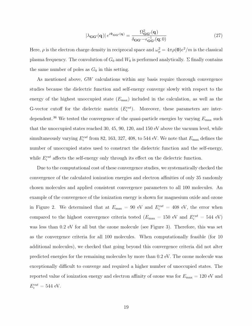
|λGG′(q)| eiΦGG′ (q) =Ω2

GG′(q)

δGG′−ε−1GG′(q; 0)

(27)

Here, ρ is the electron charge density in reciprocal space and ω2p = 4πρ(0)e2/m is the classical

plasma frequency. The convolution of G0 andW0 is performed analytically. Σ finally contains

the same number of poles as G0 in this setting.

As mentioned above, GW calculations within any basis require thorough convergence

studies because the dielectric function and self-energy converge slowly with respect to the

energy of the highest unoccupied state (Emax) included in the calculation, as well as the

G-vector cutoff for the dielectric matrix (Ecutε ). Moreover, these parameters are inter-

dependent.36 We tested the convergence of the quasi-particle energies by varying Emax such

that the unoccupied states reached 30, 45, 90, 120, and 150 eV above the vacuum level, while

simultaneously varying Ecutε from 82, 163, 327, 408, to 544 eV. We note that Emax defines the

number of unoccupied states used to construct the dielectric function and the self-energy,

while Ecutε affects the self-energy only through its effect on the dielectric function.

Due to the computational cost of these convergence studies, we systematically checked the

convergence of the calculated ionization energies and electron affinities of only 35 randomly

chosen molecules and applied consistent convergence parameters to all 100 molecules. An

example of the convergence of the ionization energy is shown for magnesium oxide and ozone

in Figure 2. We determined that at Emax = 90 eV and Ecutε = 408 eV, the error when

compared to the highest convergence criteria tested (Emax = 150 eV and Ecutε = 544 eV)

was less than 0.2 eV for all but the ozone molecule (see Figure 3). Therefore, this was set

as the convergence criteria for all 100 molecules. When computationally feasible (for 10

additional molecules), we checked that going beyond this convergence criteria did not alter

predicted energies for the remaining molecules by more than 0.2 eV. The ozone molecule was

exceptionally difficult to converge and required a higher number of unoccupied states. The

reported value of ionization energy and electron affinity of ozone was for Emax = 120 eV and

Ecutε = 544 eV.

19

0!

0.1!

0.2!

0.3!

0.4!

0.5!

0.6!

0.7!

150! 250! 350! 450! 550! 650!

Ozone!Magnesium oxide!

Ioni

zatio

n En

ergy

diff

eren

ce fr

om m

axim

um (e

V)!

Dielectric function cutoff (eV)! Energy of highest band (eV)!

0.0!

0.1!

0.2!

0.3!

0.4!

0.5!

0.6!

0.7!

30! 60! 90! 120!

Figure 2: The convergence behavior of the BGW-GPP ionization energy of ozone and mag-nesium oxide. The left panel shows convergence with respect to dielectric function cutoffwith the number of unoccupied states fixed such that it spans 90 eV above the vacuum level,while the right panel shows the convergence with respect to number of states for a dielectricfunction cutoff of 408 eV. The energy is given as a difference with respect to the highestconvergence criteria.

In our pseudopotentials for transition metal atoms, semi-core d-states are explicitly

treated as valence. Here, the density that is used to construct the plasma frequency does

not include the semi-core, but inclusion of semi-core electrons is necessary for describing the

nodal structure of the valence wavefunction.97 Because the planewave cutoff is very high with

use of semi-core states, we performed a limited convergence study for Cu2 of the influence

of dielectric function cutoffs and number of bands. We estimate an error of ∼0.3 eV for

the predicted ionization energies and electron affinities of these transition metal-containing

compounds.

3.2 Basis sets

Type of local basis sets: The G0W0 QP-energies in TURBOMOLE and FHI-aims are

calculated using the TURBOMOLE def2 basis sets of contracted Gaussian orbitals.98 In the

TURBOMOLE calculations the contracted Gaussians are treated analytically, exploiting

the standard properties of Gaussian functions. With FHI-aims in contrast, the Gaussian

orbitals are treated numerically to be compliant with the numeric atom-centered orbital

20

0 0.05 0.1 0.15 0.2 0.25Error (eV)

0

2

4

6

8

10

12

Coun

t

Figure 3: The number of molecules for which the estimated convergence error associatedwith the chosen Emax and Ecut

ε is within a given interval (given in eV). The estimated erroris the difference between the highest convergence parameter tested and the parameter usedfor all 100 molecules.

(NAO) technology of FHI-aims.39,55 NAOs are of the form

ϕi(r) =ui(r)

rYlm(Ω), (28)

where ui(r) are the numerically tabulated radial functions and Ylm(Ω) spherical harmonics.

In appendix A we provide a convergence study for the most critical numerical parameters

in TURBOMOLE and FHI-aims for four representative molecules. The quantities that only

depend on the occupied KS-reference states, the KS-energies, the (matrix elements of the)

exchange-correlation potentials and the exchange part of the self-energy Σx are converged at

the meV level and agree between FHI-aims and TURBOMOLE at this level. The correlation

part of the self-energy Σc depends also on the unoccupied states and introduces additional

convergence parameters that depend on the method that is used to calculate it. Their

convergence will therefore be discussed separately. Since the ground state quantities obtained

with TURBOMOLE and FHI-aims are practically identical we will conduct a basis-set

convergence study for the ground state only once using results obtained with TURBOMOLE.

21

-0,5 0

IE difference [eV]

0

10

20

30

40

50

60

Nu

mber

of

mole

cu

les

-0,5 0

IE difference [eV]

-0,5 0

IE difference [eV]

SVP TZVP QZVP

Figure 4: Histogram of the deviation of the KS-HOMO energies in the GW100 set calculatedwith the def2-SVP (left), def2-TZVP (center), and def2-QZVP (right) basis-sets from theextrapolated complete basis set limit using TURBOMOLE. The raw data can be found inthe supplemental material. The extrapolated results are obtained by linear extrapolation ofthe def2-TZVP and def2-QZVP results as a function of the reciprocal of the number of basisfunctions.

Convergence of the KS-states in the local basis-sets (DFT): The convergence of

the KS-HOMO with respect to the size of the basis set is presented in Fig. 4. The KS-

eigenvalues calculated with def2-SVP, def2-TZVP, and def2-QZVP basis sets are compared

to the ’complete’ basis-set extrapolation. The extrapolation is obtained from the def2-TZVP

and def2-QZVP results by a linear regression against the reciprocal of the total number of

basis functions. This extrapolation technique was applied previously in Ref. 48 and described

and validated there in more detail. The KS energies converge systematically with increasing

basis set size (see Appendix A.1). The molecules containing fifth row elements are excluded

from the studies since there are no all electron SVP and TZVP basis sets are available for

these elements.

Most molecules are seen to converge from below. At the QZVP level the KS energies of

66 (88) out of the 100 molecules are converged to within 50 meV (100 meV). We note that

the def2 basis sets are optimized for Hartree-Fock total energies. There convergence for KS

eigenvalues might thus be slower.

Convergence of the QP-states in the local basis sets (G0W0): The convergence of

the QP-energies with respect to the size of the basis sets is illustrated in Fig. 5 and 6. In

22

-1 -0,5 00

10

20

30

40

50

Nu

mb

er o

f m

ole

cule

s

-1 -0,5 0

HOMO orbital energy difference [eV]

-1 -0,5 0

SVP TZVP QZVP

-3 -2 -1 0 10

10

20

30

40

50

Nu

mber

of

mole

cule

s

-3 -2 -1 0 1

LUMO orbital energy difference [eV]

-3 -2 -1 0 1

SVP TZVP QZVP

Figure 5: Histogram of the deviation of the QP-HOMO and QP-LUMO energies of theGW100 set calculated with the def2-SVP (left), def2-TZVP (center) and def2-QZVP (right)basis from the extrapolated complete basis set limit using TURBOMOLE. The extrapolatedresults are obtained by linear extrapolation of the def2-TZVP and def2-QZVP results as afunction of the reciprocal of the number of basis functions.

23

the upper part of Fig. 5 we report the difference of the QP-HOMO energies to the basis-set

extrapolated results for the def2-SVP, def2-TZVP, and def2-QZVP basis sets. The QP-

LUMOs are shown in the lower part of Fig. 5. For the QP-HOMO levels the same data

is replotted in Fig. 6 as a scatter plot. All results have been calculated with FHI-aims.

TURBOMOLE gives identical results (see Sec. 4). As expected, the QP energies converge

slower with basis size than the Kohn-Sham energies. For the QP-LUMO levels we observe a

similar pattern (see Fig. 5). However, the deviations are approximately a factor 2 larger for

each basis set.

When comparing the QP-results between the local orbital codes FHI-aims and TURBO-

MOLE and the plane wave code BerkeleyGW in the results section we will always used the

extrapolated values. These will be referred to as ’EXTRA’.

0,001 0,01 0,1

1/Nbasis

-2,00

-1,50

-1,00

-0,50

0,00

0,50

εQ

P

H(e

xtr

a)-

εQ

P

H(b

asi

s) [

eV

]

SVPTZVPQZVP

Figure 6: The deviation of the QP-HOMO energies from the extrapolated complete basisset limit for the def2-SVP, def2-TZVP and def2-QZVP basis sets as a function of the inversenumber of basis functions. The results have been obtained with TURBOMOLE.

Auxiliary basis-sets: The G0W0 implementations in TURBOMOLE and FHI-aims make

use of the resolution-of-identity (RI) technique to compute four-center Coulomb integrals of

24

the type:

(ij|kl) =

∫ϕi(r)ϕj(r)ϕk(r

′)ϕl(r′)

|r− r′|drdr′ . (29)

To avoid the numerical cost associated with the computation and storage of the (ij|kl)

matrix, an auxiliary basis set Pµ is introduced to expand the product of basis function

pairs as:

ϕi(r)ϕj(r) 'Naux∑µ=1

CµijPµ(r) , (30)

where Cµij are the expansion coefficients, and Naux is the number of auxiliary basis functions

Pµ. The G0W0 equations can be conveniently rewritten employing Eq. 30 as described in

detail in Refs.39,48

In our experience, RI speeds up DFT calculations by an order of magnitude in TUR-

BOMOLE. For G0W0, the computational effort is reduced by an order of magnitude for

calculations with ∼100 basis functions. In addition, the scaling reduces from N5 to N4 or

better (where N is the number of atoms) up to 1000 basis functions.48 For G0W0 in FHI-aims,

RI is essential.39 The scaling of G0W0 in FHI-aims is always N4 or better.

The auxiliary basis functions in TURBOMOLE are supplied in a database.99,100 They

are designed such that the RI-induced error lies in the meV regime for DFT total energy

calculations.100 An important difference to FHI-aims is that the auxiliary basis functions in

FHI-aims are constructed on the fly39 and are not predefined as in TURBOMOLE.

We define the G0W0 RI error as the difference between the QP energies calculated with

and without applying RI in all steps of the calculation. This comparison is shown in Fig. 7

for TURBOMOLE using a subset of GW100. We observe that G0W0 is more sensitive to

the RI approximation than DFT with local or semi local functionals. In an earlier study we

found for a smaller set of molecules that the G0W0 RI error for the QP-HOMO energies is

below 0.1 eV.48 The same trend is observed here, see Fig. 7. Only very small systems, such as

25

helium and hydrogen, tend to have a larger G0W0 RI error of 0.24 and 0.13 eV, respectively.

In the FHI-aims calculations the parameters for constructing the auxiliary basis-sets are

chosen such that the quasiparticle energies agree with the RI-free TURBOMOLE values to

better than 1 meV compared for all systems (see also Tab. 2).

0 0.005 0.01 0.015 0.02 0.025 0.031 / NBF

0

0.05

0.1

0.15

0.2

0.25

RI

Err

or

(eV

)

H2

Ne

He

F2

FH

Kr

LiH

Figure 7: The G0W0 RI error of the QP-HOMO energies in the TURBOMOLE calculations.The RI error for the G0W0 calculations is defined as the difference between the QP-energiescalculated with and without applying the Resolution of the Identity approach at all steps ofthe calculation.

Convergence in the plane-wave basis: The BerkeleyGW 56 package computes the di-

electric function and self energy within a plane-wave basis set. The input DFT-PBE eigenval-

ues are computed with the Quantum Espresso Package,101 with a plane-wave wave-function

cutoff defined such that the total DFT-PBE energy is converged to < 1 meV/atom. The

wave-function cutoffs for all 100 molecules are presented in Appendix B, Tab. 16. Typical

values between 50 and 120 Ry are sufficient, but in some cases even 300 Ry are necessary.

The molecules are placed in a large supercell that is twice the size necessary to contain 99.9%

of the charge density. To avoid spurious interactions between periodic images at the G0W0

step, the Coulomb potential is truncated at half of the unit cell length.56

26

The KS eigenvalues computed with Quantum Espresso agree well with TURBOMOLE

and FHI-aims (see Tab. 14 in SI). In most cases the deviation is well below 0.1 eV, the mean

absolute deviation is 0.048 eV with the extrapolated and 0.045 eV with the QZVP results.

mean deviation. The largest discrepancies, in the order of 0.1 eV, occur almost exclusively

in Fluor containing molecules.

As alluded to in Sec. 3, we obtain the QP-energies by solving the QP-equation repeated

here for convenience

εQPnσ = εKS

nσ + 〈nσ|Σσx + Σσ

c (εQPnσ )− vxc|nσ〉 . (31)

We observe that also Σσx−vxc differs by less than 50 meV for the GW100 molecules between

the three codes (see Tab. 14 in SI).

The response function in the local basis: Due to the compactness of the basis in

TURBOMOLE and FHI-aims the response function can be treated in the full Hilbert space

of the def2-QZVP basis for all molecules in GW100 . Even for the smallest molecules,

the def2-QZVP basis describes a homogeneous excitation spectrum up to 350 eV. For all

molecules with more than 4 electrons, the excitation spectrum ranges well beyond 800 eV.

We tested that at least states up to 400 eV are required in the construction of Σ (i.e. in

the sum over m in Eq. 17), for all systems. The QP-HOMO energies are then converged

to within 0.05 eV. For states with energies higher than 400 eV the denominator in Eq. 17

becomes large enough to suppress further contributions.

We mention this assessment here to estimate the contribution of higher lying states in

G0W0. In practice we always include all states of the Hilbert space spanned by the chosen

basis set in our TURBOMOLE and FHI-aims calculations.

27

3.3 Treatment of core electrons

In the FHI-aims and TURBOMOLE calculations all electrons have been taken into account

explicitly at each step of the calculation. They are included fully in the KS and the G0W0

calculations and thus also take part in the screening.

3.3.1 Pseudo potentials

In the BerkeleyGW calculations we employed Troullier-Martins norm-conserving pseudopo-

tentials.102 For all atoms except the transition metals, the pseudopotentials were taken from

version 0.2.5 of the Quantum Espresso pseudopotential library.103 For Ti, Cu, and Ag, we

found it necessary to include semi-core states in the pseudopotential, to properly describe the

valence orbitals near the core.104 For Cu and Ag, we use the pseudopotentials of Hutter and

co-workers105,106 in which 19 valence electrons are treated explicitly. For Ti, we generated

the pseudo potential using the FHI98pp package,74 treating 12 electrons as valence. The

plane-wave cutoff is set such that total DFT energies are converged to 10 meV/atom and the

DFT HOMO energies are converged to 50 meV for all molecules. As shown in Figure 8, the

HOMO energies are converged to < 5 meV for the majority of the molecules (79 molecule).

The error is computed as the difference between the converged cutoff energy and a cutoff

of 120 Ry. For cases where the converged cutoff energy is determined to be greater than

120 Ry, the error is estimated as the difference between this value and a planewave cutoff

which is increased by 10 Ry. The core radii cutoff for the pseudopotentials are listed in

the Appendix B, Table 15. The wavefunction cutoff for all 100 molecules are presented in

Appendix B, Table 16. This same planewave cutoff is used at the GW step.

3.4 The quasiparticle equation

The final technical step of a G0W0 calculation is the solution of the quasi-particle equation.

Once the G0W0 self-energy is obtained, the quasi-particle energies εQPn are calculated by

28

0!

10!

20!

30!

40!

50!

60!

<1!

1-5!5-10!

10-15!

15-20!

20-25!

25-30!

30-35!

35-40!

40-45!

Cou

nt!

Error (meV)!

Figure 8: The error in the computed DFT HOMO eigenvalues due to the chosen planewavecutoff. As noted in the text, the error is calculated as the orbital energy difference fora calculation that employs the chosen cutoff and 120 Ry cutoff. If the converged cutoffis greater than or equal to 120 Ry, the error is determined as the difference between theconverged value and 10 Ry higher than this value.

solving the diagonal quasi-particle equation (Eq. 7) repeated here for convenience

εQPnσ = εKS

nσ + 〈nσ|Σ(εQPnσ )− vxc|nσ〉 . (32)

Here εKSnσ are the Kohn-Sham eigenvalues (computed in PBE in this work). Equation 32 is

generally solved iteratively due to the interdependence of the self-energy Σ(εQPnσ ) and the

quasiparticle energy εQPnσ . In most cases εQP

nσ falls in a region in which the self-energy has

no poles making it featureless and almost constant. Then the solution is unique in the

region of interest and Eq. 32 may even be linearized so a single evaluation of Σ at the KS-

energy is sufficient and there is no iteration process. In BerkeleyGW GPP calculations, the

quasiparticle equation is always linearized. This is justified since the GPP self-energy is

smooth near the quasiparticle energy.

In some cases, however, the initial KS-energy is close to a pole of Σ and as a result

29

-18 -17 -16 -15 -14 -13 -12 -11 -10 -9 -8-3

-2

-1

0

1

2

3

4

5

<HO

MO

|(E

)|HO

MO

>

(eV)

C( ) - KS+VXC- X

-15 -14 -13 -12 -11 -10 -9 -8-10

-8

-6

-4

-2

0

2

4

6

8

10

<HO

MO

|(

)|HO

MO

>

c( ) - KS + VXC - c

Figure 9: Schematic of a graphical solution of the quasi-particle equation (Eq. 32). Allintersections of the red line with the correlation part of the self-energy (black line) aresolutions of the quasi-particle equation. The left figure shows the most common situationwith a clear single solution near KS startingpoint, the right figure shows the situation thatcan lead to multiple solutions

Eq. 32 has more than one solution. These solutions are relatively close in energy, which

implies that the correction to the KS eigenvalue is not unique. A schematic example is

shown in Fig. 9. In practice, most available G0W0 codes search for a single solution of the

quasi-particle equation, only. Which solution is found depends on the initialization and the

type of the iterative procedure. In general, different codes might find different solutions to

the non-linear quasi-particle equation even though the self-energy is similar. We expect all

solutions to be physically relevant, in principle. However, which one is actually physically

relevant depends, e.g., on the quasiparticle weight (i.e. the pole residue) and furthermore

may also depend on the physical observable one would like to study.

Generically, one expects those solutions with the largest quasi-particle peak Z/(ω−εQPnσ ),

the so-called Z-factor

Znσ =1

1− ∂∂ω〈nσ|Σσ(ω)|nσ〉

∣∣ω=εQP

nσ

. (33)

to be most important. Especially very close to the poles, the slope of Σ at the quasi-particle

energy is large, Z is small and the weight of the quasi-particle peak in the spectral function

is reduced. The remaining weight is shifted to the other solutions, in case of multiple

solutions, or the incoherent background. Solutions that result from intersections with the

30

almost vertical lines when a pole in Σ changes sign are spurious in a sense. For the molecules

considered here, these poles are very sharp, as we will demonstrate in the results section.

The slope is thus almost infinite and the corresponding weight will go to zero. A lesser Padé

approximant or large damping η as often applied in a full frequency treatment will broaden

the pole and can give rise to a non-vanishing spurious Z-factor. At this point we will refrain

from further analysis of the role of the different solutions for physical observables. In this

work we ascribe the solution with the highest energy to the QP-HOMO.

One may conclude now that states whose derivative of the self-energy is large at the quasi-

particle energy, i.e. that have a small Z-factor, might lend themselves to multi-solution

behavior. If a small Z-factor is detected, it might indeed be necessary to test whether

the solution of the quasi-particle equation actually corresponds to the highest in energy

intersection between the ∆(ω) and Σ(ω). A small Z-factor, however, is not always an

indication for multi-solution behavior. We will see examples of this below.

4 Results

In the following we present our numerical assessment of the G0W0 implementations in TUR-

BOMOLE, FHI-aims, and BerkeleyGW. We have chosen the energies of the highest occupied

molecular orbital (QP-HOMO, εQPH ) and lowest unoccupied molecular orbital (LUMO, εQP

L )

as our main observables in this comparison. Both have a well defined physical meaning,

−εQPH corresponds to the first vertical ionization energy and −εQP

L is the electron affinity.

For most molecules in the GW100 set, the quasi-particle equation yields a unique solution

for the QP-HOMO and the QP-LUMO. However, four molecules exhibit the aforementioned

multi-solution behavior described in Sec. 3.4. Section 4.1.1 reports all solutions for these

four molecules in detail. In the final subsection of the results section we will then make a

comparison to other G0W0 results that are available in the literature.

31

4.1 Ionization energies

Table 2 presents the G0W0@PBE QP-HOMO energies for the molecules of the GW100 set.3

For brevity we have introduced the following abbreviations in this section: AIMS-2P for a

two pole fit in FHI-aims and AIMS-P16 and AIMS-P128 for a 16 and 128 parameter Padé

fit in FHI-aims, BGW-GPP and BGW-FF for the generalized plasmon model and the full-

frequency treatment in BerkeleyGW, and TM-RI and TM-noRI for the RI and the RI-free

treatment in TURBOMOLE. EXTRA denotes extrapolated local orbital results obtained by

extrapolating the def2-TZVP and QZVP values calculated using FHI-aims, see Section 3.2.

The TURBOMOLE noRI and the BerkeleyGW FF calculations are computationally very

demanding. They have therefore only been performed for subsets of the GW100 set (see

Tab. 2 and 5).

Table 2: The IP’s (minus the QP-HOMO energies) of the GW100 set calculated withG0W0@PBE using TURBOMOLE, FHI-aims, and BerkeleyGW. The first column denotesthe molecule’s index. The AIMS-2P, AIMS-P16, TM-RI, and TM-noRI results have beencalculated with a def2-QZVP basis. Extrapolated AIMS-P16 results, see Section 3.2, areshown in column EXTRA. The AIMS values marked with † are calculated using a 128parmeter Padé fit. The experimental geometries are taken from the references listed behindeach molecule. The experimental ionization energies, taken from the NIST database,107 arereported for comparison. Experimental values marked * correspond to vertical ionizationenergies.

Name Formula AIMS-2P AIMS-P16 BGW-GPP BGW-FF TM-RI TM-noRI EXTRA EXP

1 Helium He 23.44 23.48 24.10 - 23.24 23.48 23.49 24.59

2 Neon Ne 20.45 20.38 21.35 - 20.26 20.38 20.33 21.56

3 Argon Ar 15.07 15.13 15.94 - 15.04 15.13 15.28 15.76

4 Krypton Kr 13.49 13.57 14.00 - 13.55 13.57 13.89 14.00

5 Xenon Xe 12.03 12.02 12.08 - 11.97 12.02 - 12.13

6 Hydrogen108 H2 15.81 15.81 16.23 - 15.68 15.82 15.85 15.43

7 Lithium dimer108 Li2 5.14 4.99 5.43 - 4.98 4.99 5.05 4.73

8 Sodium dimer108 Na2 5.04 4.83 5.03 - 4.82 4.85 4.88 4.89

Continues on next page

3For a subset of the molecules considered in this work, the G0W0@PBE ionization energies – evaluatedwith the three codes – have been reported in previous publications.36,39,48 The results presented in Tab. 2show small numerical differences for some of these molecules. The deviations of these values to previouslypublished data are generally smaller than 0.1 eV, and can be mainly attributed to the different (larger) basissets employed in the present study. Furthermore, in the previous TURBOMOLE calculations we added anexchange-correlation kernel to the RPA response function and the quasi-particle equation was linearized. Theonly molecule previously calculated with BerkeleyGW is benzene, for which there is no difference betweenour current and the previous calculation.

32

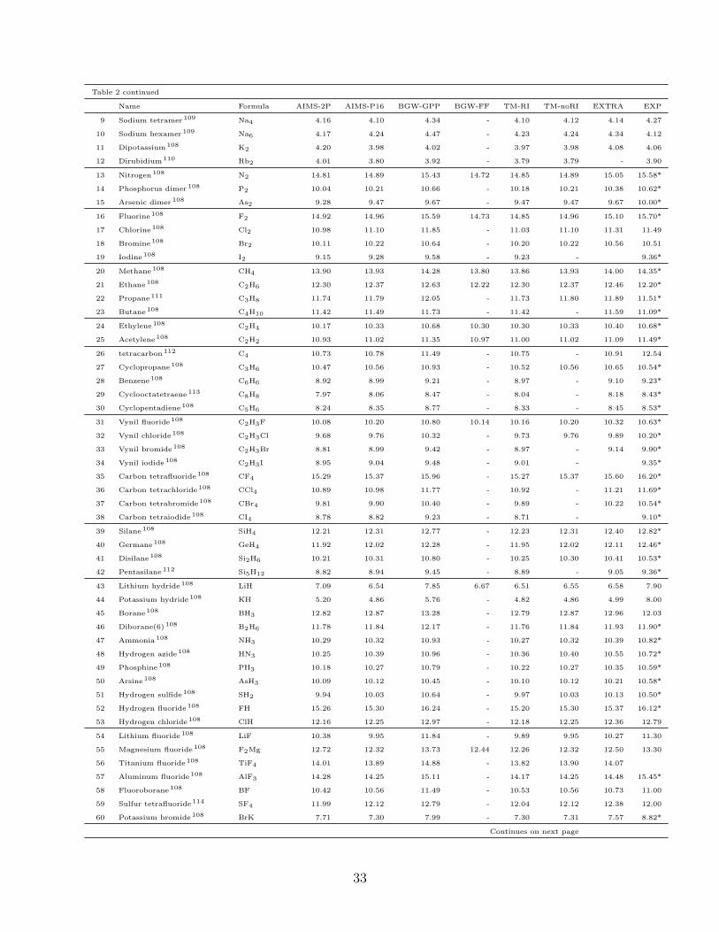
Table 2 continued

Name Formula AIMS-2P AIMS-P16 BGW-GPP BGW-FF TM-RI TM-noRI EXTRA EXP

9 Sodium tetramer109 Na4 4.16 4.10 4.34 - 4.10 4.12 4.14 4.27

10 Sodium hexamer109 Na6 4.17 4.24 4.47 - 4.23 4.24 4.34 4.12

11 Dipotassium108 K2 4.20 3.98 4.02 - 3.97 3.98 4.08 4.06

12 Dirubidium110 Rb2 4.01 3.80 3.92 - 3.79 3.79 - 3.90

13 Nitrogen108 N2 14.81 14.89 15.43 14.72 14.85 14.89 15.05 15.58*

14 Phosphorus dimer108 P2 10.04 10.21 10.66 - 10.18 10.21 10.38 10.62*

15 Arsenic dimer108 As2 9.28 9.47 9.67 - 9.47 9.47 9.67 10.00*

16 Fluorine108 F2 14.92 14.96 15.59 14.73 14.85 14.96 15.10 15.70*

17 Chlorine108 Cl2 10.98 11.10 11.85 - 11.03 11.10 11.31 11.49

18 Bromine108 Br2 10.11 10.22 10.64 - 10.20 10.22 10.56 10.51

19 Iodine108 I2 9.15 9.28 9.58 - 9.23 - 9.36*

20 Methane108 CH4 13.90 13.93 14.28 13.80 13.86 13.93 14.00 14.35*

21 Ethane108 C2H6 12.30 12.37 12.63 12.22 12.30 12.37 12.46 12.20*

22 Propane111 C3H8 11.74 11.79 12.05 - 11.73 11.80 11.89 11.51*

23 Butane108 C4H10 11.42 11.49 11.73 - 11.42 - 11.59 11.09*

24 Ethylene108 C2H4 10.17 10.33 10.68 10.30 10.30 10.33 10.40 10.68*

25 Acetylene108 C2H2 10.93 11.02 11.35 10.97 11.00 11.02 11.09 11.49*

26 tetracarbon112 C4 10.73 10.78 11.49 - 10.75 - 10.91 12.54

27 Cyclopropane108 C3H6 10.47 10.56 10.93 - 10.52 10.56 10.65 10.54*

28 Benzene108 C6H6 8.92 8.99 9.21 - 8.97 - 9.10 9.23*

29 Cyclooctatetraene113 C8H8 7.97 8.06 8.47 - 8.04 - 8.18 8.43*

30 Cyclopentadiene108 C5H6 8.24 8.35 8.77 - 8.33 - 8.45 8.53*

31 Vynil fluoride108 C2H3F 10.08 10.20 10.80 10.14 10.16 10.20 10.32 10.63*

32 Vynil chloride108 C2H3Cl 9.68 9.76 10.32 - 9.73 9.76 9.89 10.20*

33 Vynil bromide108 C2H3Br 8.81 8.99 9.42 - 8.97 - 9.14 9.90*

34 Vynil iodide108 C2H3I 8.95 9.04 9.48 - 9.01 - 9.35*

35 Carbon tetrafluoride108 CF4 15.29 15.37 15.96 - 15.27 15.37 15.60 16.20*

36 Carbon tetrachloride108 CCl4 10.89 10.98 11.77 - 10.92 - 11.21 11.69*

37 Carbon tetrabromide108 CBr4 9.81 9.90 10.40 - 9.89 - 10.22 10.54*

38 Carbon tetraiodide108 CI4 8.78 8.82 9.23 - 8.71 - 9.10*

39 Silane108 SiH4 12.21 12.31 12.77 - 12.23 12.31 12.40 12.82*

40 Germane108 GeH4 11.92 12.02 12.28 - 11.95 12.02 12.11 12.46*

41 Disilane108 Si2H6 10.21 10.31 10.80 - 10.25 10.30 10.41 10.53*

42 Pentasilane112 Si5H12 8.82 8.94 9.45 - 8.89 - 9.05 9.36*

43 Lithium hydride108 LiH 7.09 6.54 7.85 6.67 6.51 6.55 6.58 7.90

44 Potassium hydride108 KH 5.20 4.86 5.76 - 4.82 4.86 4.99 8.00

45 Borane108 BH3 12.82 12.87 13.28 - 12.79 12.87 12.96 12.03

46 Diborane(6)108 B2H6 11.78 11.84 12.17 - 11.76 11.84 11.93 11.90*

47 Ammonia108 NH3 10.29 10.32 10.93 - 10.27 10.32 10.39 10.82*

48 Hydrogen azide108 HN3 10.25 10.39 10.96 - 10.36 10.40 10.55 10.72*

49 Phosphine108 PH3 10.18 10.27 10.79 - 10.22 10.27 10.35 10.59*

50 Arsine108 AsH3 10.09 10.12 10.45 - 10.10 10.12 10.21 10.58*

51 Hydrogen sulfide108 SH2 9.94 10.03 10.64 - 9.97 10.03 10.13 10.50*

52 Hydrogen fluoride108 FH 15.26 15.30 16.24 - 15.20 15.30 15.37 16.12*

53 Hydrogen chloride108 ClH 12.16 12.25 12.97 - 12.18 12.25 12.36 12.79

54 Lithium fluoride108 LiF 10.38 9.95 11.84 - 9.89 9.95 10.27 11.30

55 Magnesium fluoride108 F2Mg 12.72 12.32 13.73 12.44 12.26 12.32 12.50 13.30

56 Titanium fluoride108 TiF4 14.01 13.89 14.88 - 13.82 13.90 14.07

57 Aluminum fluoride108 AlF3 14.28 14.25 15.11 - 14.17 14.25 14.48 15.45*

58 Fluoroborane108 BF 10.42 10.56 11.49 - 10.53 10.56 10.73 11.00

59 Sulfur tetrafluoride114 SF4 11.99 12.12 12.79 - 12.04 12.12 12.38 12.00

60 Potassium bromide108 BrK 7.71 7.30 7.99 - 7.30 7.31 7.57 8.82*

Continues on next page

33

Table 2 continued

Name Formula AIMS-2P AIMS-P16 BGW-GPP BGW-FF TM-RI TM-noRI EXTRA EXP

61 Gallium monochloride108 GaCl 9.54 9.55 10.24 - 9.53 9.55 9.74 10.07*

62 Sodium chloride108 NaCl 8.54 8.10 9.60 - 8.06 8.10 8.43 9.80*

63 Magnesium chloride108 MgCl2 11.05 10.99 11.98 - 10.95 10.99 11.20 11.80*

64 Aluminum iodide108 AlI3 9.28 9.32 9.67 - 9.30 - 9.66*

65 Boron nitride108 BN 11.19 11.03† 12.19 9.68 11.00 11.01 11.15

66 Hydrogen cyanide108 NCH 13.13 13.21 13.87 - 13.19 13.21 13.32 13.61*

67 Phosphorus mononitride108 PN 11.03 11.14 12.13 - 11.10 11.14 11.29 11.88

68 Hydrazine108 H2NNH2 9.25 9.28 9.78 9.10 9.23 9.28 9.37 8.98*

69 Formaldehyde108 H2CO 10.32 10.33 11.02 - 10.25 10.33 10.46 10.89*

70 Methanol108 CH4O 10.50 10.56 11.14 - 10.49 10.56 10.67 10.96*

71 Ethanol115 C2H6O 10.12 10.16 10.57 - 10.09 - 10.27 10.64*

72 Acetaldehyde108 C2H4O 9.59 9.55 10.16 9.43 9.48 9.55 9.66 10.24*

73 Ethoxy ethane116 C4H10O 9.30 9.32 9.70 - 9.27 - 9.42 9.61*

74 Formic acid108 CH2O2 10.78 10.73 11.39 - 10.67 10.73 10.87 11.50*

75 Hydrogen peroxide108 HOOH 10.92 10.99 11.58 10.82 10.90 10.99 11.10 11.70*

76 Water108 H2O 11.92 11.97 12.75 11.68 11.89 11.97 12.05 12.62*

77 Carbon dioxide108 CO2 13.04 13.25 13.81 13.17 13.18 13.25 13.46 13.77*

78 Carbon disulfide108 CS2 9.62 9.75 10.37 - 9.70 9.75 9.95 10.09*

79 Carbon oxysulfide108 OCS 10.73 10.91 11.49 11.02 10.86 10.91 11.11 11.19*

80 Carbon oxyselenide108 OCSe 10.08 10.20 10.55 - 10.18 - 10.43 10.37*

81 Carbon monoxide108 CO 13.37 13.57 14.33 - 13.53 13.57 13.71 14.01*

82 Ozone108 O3 11.91 11.39† 13.05 12.00 11.92 11.39 11.49 12.73*

83 Sulfur dioxide108 SO2 11.74 11.82 12.55 - 11.76 11.82 12.06 12.50*

84 Beryllium monoxide108 BeO 9.35 8.58† 10.66 9.68 9.61 8.62 8.60 10.10

85 Magnesium monoxide108 MgO 7.03 6.68† 8.51 7.08 6.66 6.66 6.75 8.76

86 Toluene108 C7H8 8.48 8.61 8.97 - 8.59 - 8.73 8.82*

87 Ethylbenzene112 C8H10 8.44 8.55 8.92 - 8.54 - 8.66 8.77*

88 Hexafluorobenzene111 C6F6 9.43 9.49 10.04 - 9.45 - 9.74 10.20*

89 Phenol108 C6H5OH 8.28 8.37 8.72 - 8.34 - 8.51 8.75*

90 Aniline108 C6H5NH2 7.61 7.64 7.98 - 7.62 - 7.78 8.05*

91 Pyridine108 C5H5N 9.08 9.04 9.50 - 9.01 - 9.17 9.51*

92 Guanine112 C5H5N5O 7.60 7.69 7.92 - 7.67 - 7.87 8.24*

93 Adenine112 C5H5N5O 7.92 7.98 8.35 - 7.95 - 8.16 8.48*

94 Cytosine112 C4H5N3O 8.25 8.29 8.77 - 8.26 - 8.44 8.94*

95 Thymine112 C5H6N2O2 8.58 8.71 9.19 - 8.68 - 8.87 9.20*

96 Uracil112 C4H4N2O2 9.37 9.22 9.94 - 9.17 - 9.38 9.68*

97 Urea117 CH4N2O 9.38 9.32 9.94 - 9.27 - 9.46 10.15*

98 Silver dimer118 Ag2 7.14 7.07 8.37 - 7.08 - 7.66

99 Copper dimer119 Cu2 7.54 7.55 8.33 - 7.52 7.53 7.78 7.46

100 Copper cyanide108 NCCu 9.79 9.42† 10.80 - 9.41 - 9.56

The absolute values of the differences of the approaches used in this work is reported

in Fig. 10 for all molecules considered in this work. The FHI-aims and TURBOMOLE

results are compared at the QZVP level, the BerkeleyGW results are compared to the

extrapolated results. The AIMS-P16 and TM-noRI QP-energies (green shading) generally

differ by less than 1-2 meV. There are, however, some molecules for which we observe a

34

20 40 60 80 100Molecule index

10-4

10-3

10-2

10-1

100

IE d

iffe

rence [

eV

]

EXTRA - BGW-GPPAIMS-P16 - AIMS-2PAIMS-P16 - TM-noRI

Figure 10: The absolute difference between QP-HOMO energies calculated with the differentG0W0 implementations. The FHI-aims and TURBOMOLE results are compared at theQZVP level. The BerkeleyGW resutls are compared to the extrapolated values. The averagesof the absolute deviations are shown as horizontal lines.

larger discrepancy. In these cases we observe a QP-weight Z in the range between 0.6 and

0.8. AIMS-P16 is slightly less accurate in these cases. For the systems for which we observe

the multi-solution behavior ( ozone (index 81), boron nitride (index 65), beryllium oxide

(index 84), and magnesium oxide (index 85)) the quasi-particle equation for the QP-HOMO

is solved close to a pole of the self-energy. As alluded to in Section 3.4, this leads to multiple

solutions of the quasiparticle equation even though the underlying self-energies show only

minor numerical differences. These cases will be discussed separately in Section 4.1.1.

As is also seen in Tab. 2 and Fig. 10, slightly larger discrepancies are observed for the

other implementations (see red and yellow shading in Fig. 10). AIMS-2P and TM-RI yield

values that are generally within 0.1 eV of the AIMS-P16 and TM-noRI results. Similarly, the

BGW-FF QP-energies agree with AIMS-P16 values within 0.2 eV, and BGW-GPP within

0.5 eV.

Table 3 condenses the information given in Fig. 10 by reporting the mean deviation

(MD) and mean absolute deviation (MAD) of the QP-HOMO energies obtained from the

different G0W0 calculations. The mean deviations reported in Tab. 3 show that TM-RI tends

to underestimate QP-HOMO, whereas the generalized plasmon pole model leads to larger

35

Table 3: Mean deviation (MD) and mean absolute deviation (MAD) between the -QP-HOMOenergies presented in Tab. 2.

MD (eV) MAD (eV)AIMS8P - AIMS2P -0.0014 0.1250AIMS8P - TM-RI 0.0456 0.0467AIMS8P - TM-noRI -0.0005 0.0032EXTRA - BGW GPP -0.4990 0.5002EXTRA - BGW FF 0.2030 0.2143

QP-HOMO values, overestimating the full-frequency-determined QP-HOMO for all systems.

The most important conclusion that can be drawn from Tabs. 2 and 3 is that the AIMS-

P16 and TM-noRI results agree to within 10 meV; the numerical aspects in these considerably

different implementations are under control. It further shows that the analytic continuation

for quasiparticle energies is very accurate, provided that a Padé fit is used and the number

of parameters is converged explicitly. We will therefore use AIMS-P16 and AIMS-P128 to

extrapolate the QP-HOMO energies to the complete basis set limit, which is also shown in

Tab. 2 in the column EXTRA. This column presents our main result, converged benchmark

numbers for the GW100 set.

There is a difference of ∼ 0.5 eV between the ionization energies from BGW-GPP and

TM or AIMS as shown in Table 3. The comparison with BGW-FF shows that the majority of

this difference arises from the GPP approximation. For the 18 molecules we tested explicitly

(discounting possible deviations arising from the multiple solution behavior), BGW-FF and

EXTRA agree to better than 0.2 eV.

4.1.1 Multiple solutions of the quasi-particle equation

The quasi-particle energies listed in Table 2 have been obtained from the solution of the non-

linear quasi-particle Eq. (32). As alluded to before, the solution for the QP-HOMO (and

QP-LUMO) is unique for the majority of the systems considered here. However, for the

QP-HOMO of ozone, boron nitride, magnesium oxide, and beryllium oxide we find multiple

36

solutions. Figure 11 illustrates the behavior for ozone for the different calculations. An

analogous plot for magnesium oxide is shown in Section 5.1 and plots for boron nitride and

beryllium oxide are reported in Appendix C. The solutions of the QP-equation are the

intersections of the red line with the self-energy curves. Table 4 reports all solutions we find

for the four multi-solution molecules.

It should be noted that technically speaking each solution of the quasiparticle equation

is potentially physically relevant. However, at least two mechanisms can be identified why

in practice usually not more than one solution needs to be considered. First, in cases with

strong broadening secondary intersections are suppressed, see, e.g., the blue trace in Fig. 11.

Second, even if the broadening is weak the slope of the self-energy at the intersection point

(i.e., the quasiparticle weight) will be different favoring in general one point against all

others. Only in intermediate situations, as appears to be the case with, e.g., ozone two or

more solutions could survive.

4.2 Electron affinities

In Table 5 we report the G0W0@PBE electron affinities for the molecules of the GW100

set. Again we present AIMS-2P, AIMS-P16, BGW-GPP, BGW-FF, TM-noRI, and TM-RI

results.

Table 5: LUMO energies in analogy to Tab. 2. The experimental electron affinities markedwith * are laser photoelectron spectroscopy values. We note, that the QP-LUMOs of thesingle atoms in the GW100 set (He-Xe) exhibit such a strong dependence on the basisset that a controlled extrapolation is not possible within the SVP, TZVP, QZVP series. Asbefore the extrapolated values are not presend for the molecules containing fifth row elementsbecause of non available SVP and TZVP all electron basis-sets.

Name Formula AIMS-2P AIMS-P16 BGW-GPP BGW-FF TM-RI TM-noRI EXTRA EXP

1 Helium He 11.01 11.01 0.44 - 11.07 11.01 - -

2 Neon Ne 11.63 11.64 0.13 - 11.65 11.64 - -

3 Argon Ar 8.08 8.11 -0.69 - 8.12 8.11 - -

4 Krypton Kr 7.61 7.63 -0.80 - 7.62 7.63 - -

Continues on next page

37

Table 5 continued

Name Formula AIMS-2P AIMS-P16 BGW-GPP BGW-FF TM-RI TM-noRI EXRTA EXP

5 Xenon Xe 7.92 7.98 0.23 - 7.96 7.98 - -

6 Hydrogen108 H2 3.50 3.50 0.26 - 3.50 3.50 3.30 -

7 Lithium dimer108 Li2 -0.67 -0.63 -0.79 - -0.61 -0.63 -0.75 -

8 Sodium dimer108 Na2 -0.61 -0.55 -0.59 - -0.50 -0.54 -0.66 0.54*

9 Sodium tetramer109 Na4 -1.09 -1.01 -1.17 - -0.99 -1.01 -1.15 0.91*

10 Sodium hexamer109 Na6 -1.07 -0.97 -1.08 - -0.94 -0.97 -1.13 -

11 Dipotassium108 K2 -0.61 -0.65 -0.72 - -0.62 -0.65 -0.75 0.50*

12 Dirubidium110 Rb2 -0.63 -0.62 -0.74 - -0.62 - - 0.50*

13 Nitrogen108 N2 2.41 2.45 2.00 - 2.47 2.45 2.12 -

14 Phosphorus dimer108 P2 -0.82 -0.72 -1.21 - -0.70 -0.72 -1.08 0.63*

15 Arsenic dimer108 As2 -0.92 -0.85 -1.12 - -0.86 -0.85 -1.52 0.74*

16 Fluorine108 F2 -0.88 -0.70 -0.41 -0.97 -0.63 -0.70 -1.23 -

17 Chlorine108 Cl2 -0.98 -0.89 -1.56 - -0.85 -0.89 -1.40 -

18 Bromine108 Br2 -1.54 -1.40 -1.93 - -1.41 -1.40 -1.96 -

19 Iodine108 I2 -1.81 -1.68 -2.17 - -2.16 - - -

20 Methane108 CH4 2.42 2.45 0.25 - 2.48 2.45 2.03 -

21 Ethane108 C2H6 2.27 2.29 0.32 - 2.32 2.29 1.93 -

22 Propane111 C3H8 2.16 2.19 0.35 - 2.23 2.19 1.87 -

23 Butane108 C4H10 2.12 2.14 0.36 - 2.18 - 1.83 -

24 Ethylene108 C2H4 1.94 2.02 1.91 - 2.04 2.02 1.82 -

25 Acetylene108 C2H2 2.81 2.86 0.19 - 2.88 2.86 2.56 -

26 tetracarbon112 C4 -3.03 -2.94 -3.20 - -2.93 - -3.15 3.88*

27 Cyclopropane108 C3H6 2.42 2.45 0.35 - 2.48 2.45 1.96 -

28 Benzene108 C6H6 0.97 1.09 1.16 - 1.10 - 0.89 -

29 Cyclooctatetraene113 C8H8 -0.01 0.06 0.04 - 0.07 - -0.12 0.65

30 Cyclopentadiene108 C5H6 0.98 1.04 1.02 - 1.06 - 0.85 -

31 Vynil fluoride108 C2H3F 2.04 2.15 2.12 2.08 2.17 2.15 1.88 -

32 Vynil chloride108 C2H3Cl 1.32 1.42 1.20 - 1.44 1.44 1.17 -

33 Vynil bromide108 C2H3Br 1.35 1.38 1.25 - 1.40 - 1.11 -

34 Vynil iodide108 C2H3I 0.82 0.89 0.47 - 0.84 - - -

35 Carbon tetrafluoride108 CF4 4.34 4.41 0.32 - 4.42 4.41 3.88 -

36 Carbon tetrachloride108 CCl4 -0.08 -0.01 -0.64 - 0.02 - -0.54 -

37 Carbon tetrabromide108 CBr4 -1.14 -1.08 -1.43 - -1.08 - -1.56 -

38 Carbon tetraiodide108 CI4 -2.22 -2.14 -2.43 - -2.11 - - -

39 Silane108 SiH4 2.48 2.51 0.09 - 2.53 2.51 2.26 -

40 Germane108 GeH4 2.12 2.30 0.04 - 2.31 2.30 1.85 -

41 Disilane108 Si2H6 1.65 1.69 0.23 - 1.72 - 1.51 -

42 Pentasilane112 Si5H12 0.07 0.16 -0.08 - 0.19 - 0.00 -

43 Lithium hydride108 LiH -0.11 -0.07 -0.37 - -0.06 -0.07 -0.16 0.34*

44 Potassium hydride108 KH -0.17 -0.18 -0.56 - -0.16 -0.18 -0.32 -

45 Borane108 BH3 0.05 0.12 -0.06 - 0.12 0.12 0.03 0.04*

46 Diborane(6)108 B2H6 0.78 0.84 0.70 - 0.85 0.84 0.74 -

47 Ammonia108 NH3 2.28 2.31 0.24 - 2.33 2.31 2.00 -

48 Hydrogen azide108 HN3 1.34 1.40 1.38 - 1.43 1.40 1.10 -

49 Phosphine108 PH3 2.46 2.50 0.03 - 2.52 2.50 2.26 -

50 Arsine108 AsH3 1.84 2.32 -0.13 - 2.34 2.32 1.94 -

51 Hydrogen sulfide108 SH2 2.52 2.56 -0.35 - 2.59 2.56 2.25 -

52 Hydrogen fluoride108 FH 2.51 2.54 0.26 - 2.55 2.54 2.04 -

53 Hydrogen chloride108 ClH 2.00 2.06 -0.45 - 2.09 2.06 1.53 -

54 Lithium fluoride108 LiF 0.09 0.09 -0.58 - 0.09 0.09 -0.01 -

55 Magnesium fluoride108 F2Mg -0.18 -0.14 -1.22 -1.18 -0.14 -0.14 -0.31 -

56 Titanium fluoride108 TiF4 -0.59 -0.60 -0.66 - -0.57 - -1.06 2.50

Continues on next page

38

Table 5 continued

Name Formula AIMS-2P AIMS-P16 BGW-GPP BGW-FF TM-RI TM-noRI EXRTA EXP

57 Aluminum fluoride108 AlF3 0.07 0.16 -0.61 - 0.17 0.16 -0.23 -

58 Fluoroborane108 BF 1.06 1.22 0.89 - 1.24 1.22 1.05 -

59 Sulfur tetrafluoride114 SF4 0.25 0.38 0.00 - 0.42 0.38 -0.10 -

60 Potassium bromide108 BrK -0.30 -0.31 -0.91 - -0.31 -0.31 -0.42 0.64*

61 Gallium monochloride108 GaCl -0.04 -0.02 -0.31 - -0.01 -0.02 -0.39 -

62 Sodium chloride108 NaCl -0.39 -0.39 -1.38 - -0.39 -0.39 -0.42 0.73*

63 Magnesium chloride108 MgCl2 -0.52 -0.43 -1.30 - -0.43 -0.43 -0.68 -

64 Aluminum iodide108 AlI3 -0.87 -0.80 -1.23 - -0.78 - - -

65 Boron nitride108 BN -3.93 -3.88 -3.99 - -3.93 -3.95 -3.95 3.16*

66 Hydrogen cyanide108 NCH 2.54 2.58 2.47 - 2.60 2.58 2.22 -

67 Phosphorus mononitride108 PN -0.30 -0.20 -0.65 - -0.18 -0.20 -0.59 -

68 Hydrazine108 H2NNH2 1.96 1.99 0.33 0.35 2.02 1.99 1.68 -

69 Formaldehyde108 H2CO 0.89 0.96 0.93 - 0.99 0.96 0.71 -

70 Methanol108 CH4O 2.22 2.25 0.42 - 2.27 2.25 1.81 -

71 Ethanol115 C2H6O 2.04 2.08 0.44 - 2.10 - 1.67 -

72 Acetaldehyde108 C2H4O 0.99 1.05 1.10 - 1.08 - 0.83 -

73 Ethoxy ethane116 C4H10O 2.07 2.10 0.36 - 2.13 - 1.70 -

74 Formic acid108 CH2O2 1.85 1.91 1.91 - 1.94 1.91 1.59 -

75 Hydrogen peroxide108 HOOH 2.21 2.35 2.17 1.95 2.40 2.35 1.95 -

76 Water108 H2O 2.33 2.37 0.26 - 2.38 2.38 2.01 -

77 Carbon dioxide108 CO2 2.45 2.50 0.25 0.28 2.50 2.50 0.93 -

78 Carbon disulfide108 CS2 -0.30 -0.20 -0.43 - -0.16 -0.20 -0.55 0.58

79 Carbon oxysulfide108 OCS 1.14 1.21 0.94 1.03 1.25 1.22 0.83 0.46

80 Carbon oxyselenide108 OCSe 0.80 0.87 0.73 - 0.90 - 0.52 -

81 Carbon monoxide108 CO 0.58 0.67 0.40 - 0.70 0.67 0.37 1.33

82 Ozone108 O3 -2.41 -2.30 -2.59 -1.87 -2.23 -2.30 -2.69 2.10*

83 Sulfur dioxide108 SO2 -1.12 -1.00 -1.24 - -0.95 -1.00 -1.49 1.11*

84 Beryllium monoxide108 BeO -2.34 -2.56 -2.80 - -2.48 -2.49 -2.72 -

85 Magnesium monoxide108 MgO -2.01 -1.89 -2.08 - -1.87 - -2.13 -

86 Toluene108 C7H8 0.94 1.01 0.95 - 1.03 - 0.83 -

87 Ethylbenzene112 C8H10 0.97 1.04 0.96 - 1.06 - 0.87 -

88 Hexafluorobenzene111 C6F6 0.61 0.66 -0.21 - 0.68 - 0.36 0.70

89 Phenol108 C6H5OH 0.88 0.96 0.93 - 0.97 - 0.74 -

90 Aniline108 C6H5NH2 1.06 1.15 1.13 - 1.16 - 0.94 -

91 Pyridine108 C5H5N 0.41 0.51 0.50 - 0.53 - 0.30 -

92 Guanine112 C5H5N5O 0.72 0.74 0.42 - 0.77 - 0.46 -

93 Adenine112 C5H5N5O 0.42 0.47 0.48 - 0.49 - 0.21 -0.54*

94 Cytosine112 C4H5N3O 0.21 0.26 0.26 - 0.28 - 0.01 -

95 Thymine112 C5H6N2O2 0.01 0.06 0.00 - 0.08 - -0.18 -0.29*

96 Uracil112 C4H4N2O2 -0.07 0.01 -0.03 - 0.03 - -0.25 -0.22*

97 Urea117 CH4N2O 1.60 1.62 0.25 - 1.64 - 1.17 -

98 Silver dimer118 Ag2 -1.06 -1.05 -1.47 - -1.20 - - 1.10*

99 Copper dimer119 Cu2 -1.21 -0.92 -1.44 - -0.75 -0.76 -1.23 0.84*

100 Copper cyanide108 NCCu -1.84 -1.65 -2.08 - -1.64 - -1.85 1.47*

The absolute value of the difference between the various calculated electron affinities are

reported in Fig. 12.

39

-15 -14 -13 -12 -11 -10 -9 -8-10

-8

-6

-4

-2

0

2

4

6

8

10 O3

<HO

MO

|(

)|HO

MO

> (e

V)

(eV)

TM -5 TM -3 BGW FF BGW GPP AIMS 128 Pade AIMS 16 pade AIMS 2p - KS + Vxc - x

Figure 11: Comparison of the energy dependent correlation part of the self-energy Σc(ε)calculated with the three different codes using different procedures for ozone. "TM -5" and"TM -3" indicate TURBOMOLE results calculated with imaginary shifts of η = 10−3 and10−5 Hartree, respectively. The intersections of these curves with the (red) line ω − εKS +Vxc − Σx correspond to the solutions of the QP-equation

40

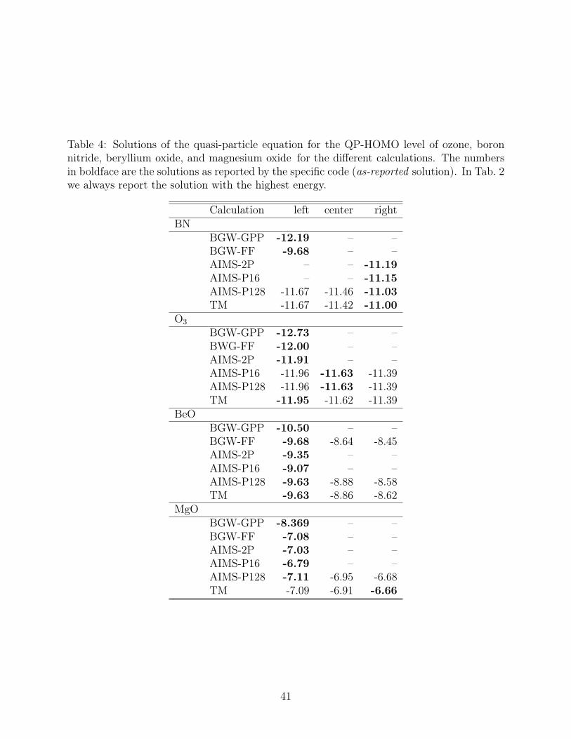
Table 4: Solutions of the quasi-particle equation for the QP-HOMO level of ozone, boronnitride, beryllium oxide, and magnesium oxide for the different calculations. The numbersin boldface are the solutions as reported by the specific code (as-reported solution). In Tab. 2we always report the solution with the highest energy.

Calculation left center rightBN

BGW-GPP -12.19 – –BGW-FF -9.68 – –AIMS-2P – – -11.19AIMS-P16 – – -11.15AIMS-P128 -11.67 -11.46 -11.03TM -11.67 -11.42 -11.00

O3

BGW-GPP -12.73 – –BWG-FF -12.00 – –AIMS-2P -11.91 – –AIMS-P16 -11.96 -11.63 -11.39AIMS-P128 -11.96 -11.63 -11.39TM -11.95 -11.62 -11.39

BeOBGW-GPP -10.50 – –BGW-FF -9.68 -8.64 -8.45AIMS-2P -9.35 – –AIMS-P16 -9.07 – –AIMS-P128 -9.63 -8.88 -8.58TM -9.63 -8.86 -8.62

MgOBGW-GPP -8.369 – –BGW-FF -7.08 – –AIMS-2P -7.03 – –AIMS-P16 -6.79 – –AIMS-P128 -7.11 -6.95 -6.68TM -7.09 -6.91 -6.66

41

20 40 60 80 100Molecule index

10-4

10-3

10-2

10-1

EA

dif

fere

nce [

eV

]

AIMS-P16 - AIMS-2PAIMS-P16 - TM-noRI

20 40 60 80 100Molecule index

10-2

10-1

100

EA

dif

fere

nce [

eV

]

EXTRA - BGW-GPPEXTRA - BGW-GPP (Bound)

Figure 12: As for Fig. 10 for the QP-LUMO.

42

Table 6: As for Table 3 for the QP-LUMO.

MD (eV) MAD(eV)AIMS8P - AIMS2P 0.0652 0.0710AIMS8P - TM-RI -0.0143 0.0302AIMS8P - TM-noRI -0.0035 0.0061EXTRA - BGW GPP 0.4399 0.6902EXTRA - BGW GPP (Bound) 0.0682 0.0725EXTRA - BGW FF 0.3133 0.4388

The analysis of the deviations in Table 6 and Fig. 12 shows trends similar to those

observed for the εQPH in Sec. 4.1. Again, the agreement between the TM-noRI and AIMS-

P16 electron affinities is of the order of a few meV. The TM-RI G0W0 implementation yields

electron affinities that are generally within 14 meV from the TM-noRI and AIMS-P16 values.

One may conclude from this that QP-energies of occupied states are more sensitive to the

RI approximation than those of unoccupied states.

In the comparison between the extrapolated data and the BGW data we observe a sig-

nificant difference between systems with a bound and an unbound LUMO state. In case of a

bound LUMO state the agreement between the EXTRA values and BGW results is similar

to that observed for the occupied states. For the unbound LUMOs the agreement can be far

off. Here the local orbital description of the unbound states clearly is not well converged.

It is noted, however, that the convergence is worst for small systems. Most molecules with

more than four none-hydrogen atoms show a small deviation also for unbound LUMOs.

4.3 Literature comparison

Table 7: G0W0@PBE literature values for QP-HOMO energies compared to the BGW-GPPand extrapolated data from this study. The second line in the header indicates whether alocal-orbital (LO) or plane-wave (PW) basis was used.

Name Formula BGW-GPP EXTRA Pham et al.44 Brunevalet al.46 Rostgaardet al.28 Qianet al.30 Other

PW LO LO PW

Lithium dimer Li2 -5.43 -5.05 - -5.12 -4.4 - -5.1418’

Sodium dimer Na2 -5.03 -4.88 - -4.89 4.7 - -5.116

Sodium tetramer Na4 -4.34 -4.14 - - - - -4.2516

Sodium hexamer Na6 -4.47 -4.34 - - - - -4.1616

Continues on next page

43

Table 7 continued

Name Formula BGW-GPP EXTRA Phamet al. Brunevalet al. Rostgaardet al. Qianet al. Other

Dipotassium K2 -4.02 -4.08 - - - - -3.8418

Nitrogen N2 -15.43 -15.05 - -14.98 -15.7 -

Phosphorus dimer P2 -10.66 -10.38 - -10.12 9 -

Fluorine F2 -15.59 -15.10 - -15.19 -16.2 -

Chlorine Cl2 -11.85 -11.31 - -11.16 -11.5 -

Methane CH4 -14.28 -14.00 - -14.03 -14.4 - 14.3120

Propane C3H8 -12.05 -11.89 -11.84 - - -

Butane C4H10 -11.73 -11.59 -11.58 - - -

Ethylene C2H4 -10.68 -10.40 - -10.37 -9.6 -

Acetylene C2H2 -11.35 -11.09 - -11.08 -11.2 -

Cyclopropane C3H6 -10.93 -10.65 -10.6 - - -

Benzene C6H6 -9.21 -9.10 -9.04 - - - -9.0386

Carbon tetrafluoride CF4 -15.96 -15.60 -15.38 - - -

Carbon tetrachloride CCl4 -11.77 -11.21 -11.22 - - -

Silane SiH4 -12.77 -12.40 - -12.4 -12.4 - -12.3086

Disilane Si2H6 -10.80 -10.41 - -10.38 -11.3 -

Lithium hydride LiH -7.85 -6.58 - -7.07 -8 -

Ammonia NH3 -10.93 -10.39 - -10.5 -10.6 - -10.719

Phosphine PH3 -10.79 -10.35 - -10.21 -10 -

Hydrogen sulfide SH2 -10.64 -10.13 - - -9.9 -

Hydrogen chloride ClH -12.97 -12.36 - -12.35 - -

Lithium fluoride LiF -11.84 -10.27 - -10.61 -12 -

Aluminum fluoride AlF3 -15.11 -14.48 -14.34 - - -

Sodium chloride NaCl -9.60 -8.43 - -8.43 -8.8 -

Hydrogen cyanide NCH -13.87 -13.32 - -13.2 - -

Hydrazine H2NNH2 -9.78 -9.37 - -9.87 -9.5 -

Formaldehyde H2CO -11.02 -10.46 - -10.51 - -

Hydrogen peroxide HOOH -11.58 -11.10 - -11.02 -11.1 -

Water H2O -12.75 -12.05 - -12.15 -11.9 -

Carbon dioxide CO2 -13.81 -13.46 - -13.32 -13.6 -

Carbon disulfide CS2 -10.37 -9.95 -9.89 - - -

Carbon oxysulfide OCS -11.49 -11.11 -11.01 - - -

Carbon monoxide CO -14.33 -13.71 - -13.55 -13.9 - -14.119

Ozone O3 -13.05 -11.49 -12.2 - - -

Sulfur dioxide SO2 -12.55 -12.06 - -11.83 -11.7 -

Pyridine C5H5N -9.50 -9.17 -9.54 - - -

Guanine C5H5N5O -7.92 -7.87 - - - -7.64

Adenine C5H5N5O -8.35 -8.16 - - - -7.99

Cytosine C4H5N3O -8.77 -8.44 - - - -8.18

Thymine C5H6N2O2 -9.19 -8.87 - - - -8.63

Uracil C4H4N2O2 -9.94 -9.38 - - - -8.99

4.3.1 Comparison with plane-wave results

A subset of the GW100 molecules has previously been calculated by Pham et al. using a

plane wave basis set.37,444 The diagonal quasi-particle equation is solved as in the present4C2H4O is present in both sets. In GW100 this is acetaldehyde, whereas in Pham et al.’s set this is

ethylene oxide.

44

work. Moreover, the analytic structure of the self-energy is take into account consistently.

These results are hence fully comparable to the results of the present paper. For seven out

of twelve of the molecules in the intersecting subset we observe an agreement within ∼0.1 eV

of our extrapolated results. The molecules containing Fluorine show a somewhat larger

discrepancy and so do ozone and pyridine (up to 0.5 eV). For ozone the slope of the self-

energy around the quasi-particle energy is steep, which implies a low quasi-particle weight

(see Section 4.1.1) and furthermore exhibits multi-solution behavior as discussed previously

and in Section 4.1.1. In pyridine the self-energy also exhibits a relatively large slope of 0.35.

However, no multi-solution behavior aggravates the solution of the quasi-particle equation.

The DNA bases have been studied by Qian et al.30 They use a planewave basis in com-

bination with a wannier-type optimized basis for the response function. The diagonal quasi-

particle equation is solved as in the present work and the self-energy is calculated using

analytic continuation. They estimate their results to be accurate to within 0.1 eV. Our

extrapolated results for G, A, C, T lie approximately 0.2 eV lower in energy (0.4 eV for

Uracil). There are two possible causes for the observed deviation. Firstly the comparison

of extrapolated results to none-extrapolated results, which tends to lower extrapolated re-

sults. The second cause is the comparison of all-electron to froze-core results. Increasing the

number of valence electrons increases the screening. This reduces the absolute size of the (in

general positive) contribution of the correlation part of the self-energy and hence lowers the

QP-energies. Both effects hence point in the direction of the observed deviation.

4.3.2 Comparison with local-orbital results

Recently, several local-orbital G0W0 implementations have emerged. We have included the

G0W0@PBE values reported with these codes28,29,31,32,39,40,43,46–49 in Tab. 7. We often observe

numerical differences that are larger than 0.1 eV, and – for some systems – of the order of

1 eV. For example, the G0W0@PBE ionization energy of the CO2 molecule has already been

studied in several other works.28,39,46,48 The reported values span a range of almost 1 eV

45

(12.8-13.6 eV, the experimental ionization energy being 13.78 eV107). For other systems, as

e.g. N2 and NH3, the published G0W0@PBE ionization energies are also distributed in a

similar energy range.

We attribute the large spread to the different basis function choices (gaussian, molecular

orbital, .. ) and sizes (triple zeta, quadruple zeta, ...) and the fact that no extrapolation to

the complete basis set limit has been performed. The different treatments of the frequency

dependence also play a role. The results reported in this work allow us to estimate the

impact of these approximations. For instance, Fig. 10 illustrates that the error of a two-pole

analytic continuation is mostly smaller than 0.12 eV. Conversely, Fig. 6 indicates that the

basis set size has a considerable impact on the ionization energies. Even for the relatively

large QZVP basis the QP-HOMO energies are underestimated by ∼0.12 eV on average.

Another factor that may affect the comparison with the published G0W0 ionization en-

ergies is the way in which the quasi-particle equation is solved. The quasi-particle energies

may be determined either from the iterative solution of Eq. 32, or alternatively, from the

linearized quasi-particle equation (see, e.g., Ref. 121). Looking at our CO2 example, it is lin-

earized in Refs 28,46,48 and solved in Ref 39. We find that the ionization energies obtained

from these two approaches may differ by up to 0.5 eV.

Summarizing, we believe that deviations up to a few hundred meV can be explained by

the technical differences in the G0W0 implementations discussed above. We mention that

the results of Rostgaard et al.28 deviate in 4 out of 22 cases by about ∼1 eV or more (up to

2 eV), which seems hard to reconcile with our general findings.

4.4 Comparison to experiment

In this work, the focus is on a methodology; we establish aG0W0@PBE benchmark result that

holds (with certain bounds) irrespective of how the G0W0 equations have been implemented.

Residual discrepancies to experimental data persist, that are typically several hundred meV,

see Table 8. Our work strongly suggests that on the theory side these discrepancies reflect (i)

46

the neglect of self-consistency and (ii) vertex corrections. (The agreement with experiment

is better for the vertical ionization energies.) For some classes of molecules an informed

choice of the starting point, e.g. B3LYP, PBE0 or static COHSEX instead of PBE, could

lead to a reduction of the discrepancies to experiment by factors of order unity (see, e.g.,

Ref.42,122). However, corrections that are applicable to broad system classes and that can

be systematically further improved upon can probably not be achieved in this way. Our

table also shows a comparison between the simplifying GPP-model and experimental data.

The comparison is favorable, at first sight, which at this point is not fully understood and a

matter of ongoing investigations.123

Table 8: Mean deviation (MD) and mean absolute deviation (MAD) between the QP-HOMOenergies presented in Tab. 2 and the experimental Ionization energies. The second half of thetable compares only those systems for which the experimental ionization energy is vertical.

MD(eV) MAD (eV)AIMS8P - EXP 0.52 0.58EXTRA - EXP 0.40 0.50GPP - EXP -0.09 0.28AIMS8P - EXP (vertical only) 0.48 0.51EXTRA - EXP (vertical only) 0.37 0.42GPP - EXP (vertical only) -0.05 0.20

5 Discussion

As discussed in Sec. 3.2 both, the KS-energies and the exchange part of the self-energy, are

well converged. Moreover, in Sec. 3.2 we have already discussed the errors introduced by the

finite basis set and additional computational approximations such as RI and the freezing of

core states. In this section, we discuss the differences between the QP-energies reported in

Tables 2 and 5 that originate from the correlation part of the GW self-energy. We start by

discussing the appearance of multiple solutions of the QP-equation and their impact on the

QP-energies. Then, we discuss the aspects that relate to different approaches to treat the

47

frequency dependence of the self-energy.

5.1 Multiple solutions of the QP-equation

For four molecules - ozone, boron nitride, beryllium oxide, and magnesium oxide - we found

multiple solutions with comparable energy for the QP-HOMO level. To illustrate this be-

havior, we showed the correlation part of the G0W0@PBE self-energy for ozone in Fig. 11.

In Fig. 13 we show that of magnesium oxide. Similar plots for boron nitride and beryllium

oxide are provided in Appendix C. For boron nitride, ∆(ω) crosses one pole of Σ(ω), which

results in three solutions. For ozone, beryllium oxide and magnesium oxide, we obtain five

solutions

Inspection of Fig. 11, 13, and 18 confirms that the multi-solution behavior typically

emerges, when the intersection is close to poles in the self-energy. For BrK, LiH, KH, copper

cyanid and Cu2 we also observe large self-energy derivatives (small Z-factors) but the poles

are not close enough to the solution of the quasi-particle equation to give rise to multiple

solutions. An example is show in Fig. 14 for copper cyanid. The slope of the self-energy is

large but rather constant between the KS-energy and the QP-energy. Any Newton-Raphson-

like algorithm to iterate the QP-equation will converge to a unique QP-energy when started

at the KS-energy. This QP-energy is, however, close to a pole, hence small differences in

the self-energy calculated by the different approaches do result in changes in the final value.

This behavior differs from the case of, e.g., magnesium oxide where the first iteration step

takes the algorithm to the other side of the first pole.

Figures. 11, 13 and 18 as well as Tab. 4 illustrate that the occurrence of multiple solutions

strongly depends on the frequency treatment of the G0W0 implementation. In general, the

GPP approach and the two pole analytic continuation gives rise to a self-energy that has too

few poles or poles that are considerably broadened. Additionally, the GPP approximation

shifts the self-energy poles away from the quasiparticle energies, resulting in higher predicted

G0W0 quasiparticle energies. The result is a slowly varying self-energy with a unique solution

48

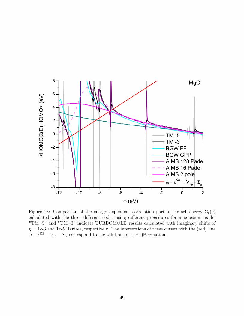
-12 -10 -8 -6 -4 -2 0 2-8

-6

-4

-2

0

2

4

6

8 MgO

<HO

MO

|(E

)|HO

MO

> (e

V)

(eV)

TM -5 TM -3 BGW FF BGW GPP AIMS 128 Pade AIMS 16 Pade AIMS 2 pole - KS + Vxc - x

Figure 13: Comparison of the energy dependent correlation part of the self-energy Σc(ε)calculated with the three different codes using different procedures for magnesium oxide."TM -5" and "TM -3" indicate TURBOMOLE results calculated with imaginary shifts ofη = 1e-3 and 1e-5 Hartree, respectively. The intersections of these curves with the (red) lineω − εKS + Vxc − Σx correspond to the solutions of the QP-equation.

49

-12 -11 -10 -9 -8 -7 -6-10

-8

-6

-4

-2

0

2

4

6

8

10CNCu

<HO

MO

|(E

)|HO

MO

>

E (eV)

TM -3 - KS+VXC- X KS

Figure 14: The energy dependent correlation part of the self-energy Σc(ε) of copper cyanidcalculated using TURBOMOLE.

50

to the quasi-particle equation in the energy region of interest. For many systems (including

many of the molecules in GW100) the true poles of Σ are sufficiently far away from the quasi-

particle energies or several poles merge into a broad pole with a gently sloped self-energy

in the energy region of interest. In these cases the GPP model and the two pole analytic

continuation can be expected to agree well with the analytic and numerical full frequency

methods (see also Section 5.2).

In case of multiple solutions, the solution that is reported by the code depends on the

iterative solver that is employed for the QP-equation. The solver in TURBOMOLE is con-

structed to always find the solution with the largest quasiparticle weight, i.e., the smallest

derivative. In FHI-aims a simple iteration is used, which sometimes yields a different so-

lution. In BerkeleyGW the QP-equation is linearized in the case of GPP and solved by

graphically finding the point where εKS + Σ− VXC is equivalent to εQP in the case of FF.

5.2 Padé, two-pole and plasmon pole approximations

For most systems the solutions of the diagonal QP-equation, Eq. (32), are found in a region

in which the self-energy is rather flat – i.e., ∂Σ/∂ε is small and the quasi-particle weight

Z = 11−∂Σ/∂ε

is close to unity. In these cases, the self-energy is only evaluated in an energy

region in which there are no poles nearby. For this purpose, a simple approximation for

the energy dependence of Σ – such as the two-pole analytic continuation – may provide

quasiparticle energies converged within 0.2 eV, as the data reported in Tab. 2 and 5 indicates.

This is further illustrated in Fig. 15 where we report the difference between the AIMS-2P

and the TM-noRI ionization energies as a function of Σ′ = ∂Σ/∂ε

For small values of Σ′ (−0.5 < Σ′ < 0), the deviation between AIMS-2P and the TM-

noRI is consistently below 0.2 eV. In this case, the two-pole analytic continuation tends

to overestimate the ionization energies by ∼0.1 eV on average. However, for Σ′ < −0.5

AIMS-2P systematically underestimates the ionization energies by 0.4-0.5 eV as compared

51

to TM-noRI.5

-2,5 -2,0 -1,5 -1,0 -0,5 0,0

∂Σ/∂ε (eV)

-0,6

-0,4

-0,2

0,0

0,2

AIM

S 2

P -

TM

no

RI

(eV

)

-2,5 -2,0 -1,5 -1,0 -0,5 0,0

∂Σ/∂ε (eV)

-2,0

-1,5

-1,0

-0,5

0,0

0,5

BG

W G

PP

- E

XT

RA

(eV

)

Figure 15: Difference between AIMS-2P and TM-noRI (left) and BGW-GPP and EXTRA(right) ionization energies as a function of ∂Σ/∂ε.

Molecules that present large derivatives ∂Σ/∂ε for the QP-HOMO level are, for instance,

BrK, LiH, KH, Cu2, NCCu, O3, BN, BeO, and MgO. Here the quasiparticle equation has

solutions close to a pole of the self-energy, as illustrated in Fig. 11, 13 and 18. As a con-

sequence, the resolution of the pole-structure of the self-energy, as achieved by different

methods, now matters more. For O3, BeO, and MgO, AIMS-P16 provides enough fitting

parameters. Conversely, for BN and CNCu it is necessary to increase the number of Padé-

parameters up to 128 to describe the poles of the self-energy sufficiently well, as illustrated

in Figs. 11 and 13 and Tab. 4.

Very smooth self-energies result from plasmon-pole models for the response function.

Besides the ’flattening’ of the correlation part of the self-energy we also observe an overall

decreased correlation part of the self-energy, see Figs. 11 and 13, that is not present in the5This shift from underestimation to overestimation can be rationalized as follows. In case of a large

derivative the solution is close to a pole of the self-energy. When this pole is not captured in a few poleapproximation the corresponding self energy will be smaller since the pole is in general situated at lowerenergy for the QP-HOMO level. As a result, the QP-energy will be underestimated, because in the fewpole scenario the intersection happens “too early”, i.e. it is too far on the left. For small derivatives, thereis no pole nearby. In the absence of a single dominant pole, the global contribution of all poles becomesvisible. The poles of the occupied levels minus the excitation energies and of the unoccupied levels at plusthe excitation energies. In a few pole approximation there will usually be more poles missing at high energythan at low energy. The missing tails of the high energy poles give a negative contribution and becauseof their larger number their absence may be causing an overestimation of the self-energy. As a result theQP-energies will be overestimated.

52

2-pole self-energy.

-1,5 -1 -0,5 0 0,5 1 1,5

IE difference [eV]

0

5

10

15

20

25

Num

ber

of

mole

cule

s

-1,5 -1 -0,5 0 0,5 1 1,5

IE difference [eV]

BGW-GPP - EXTRA BGW-FF - EXTRA

Figure 16: Deviation between the extrapolated quasi-particle energies, and BerkeleyGWevaluated in the GPP (left) and with a full frequency treatment (right).

5.3 Numerical full frequency integration

In contrast to imaginary frequency treatments and plasmon pole models, a full frequency

treatment can in principle be converged to the exact analytic G0W0 self energy by increasing

the density of the frequency grid.6 We indeed see that the FF results reproduce the pole-

positions in the analytically treated self-energy accurately (see Figures 11, 13 and 18). Even

in MgO, which features many low intensity poles, we observe this agreement for many poles-

positions. In contrast, the pole-broadening in FF is much more pronounced. This is caused

by the finite mesh size of the numerical integration, ∆ω, and the imaginary shift η (see

Eq. 18). The full frequency approach ideally requires ∆ω η. In practice, however,

∆ω . η, which introduces a considerable additional broadening. To simulate this effect

in TURBOMOLE we ran calculations with η = 0.2 eV and obtained self-energy matrix

elements almost identical with FF (not shown).

The agreement of the pole positions and the self-energy curves calculated at equal broad-6The Padé approximation could in principle, from a mathematical point of view, also be converged fully

to the analytic self-energy. However, in practice it is very hard to fit more than 64 poles to the smoothlyvarying self-energy on the imaginary axis.

53

ening η suggests that both, the plane-wave basis and the localized basis, would, in a fully

converged calculation, produce the same results. Decreasing η in Eq. 18 would, however,

necessitate a smaller ∆ω, which would increase the number of frequency points to a com-

putationally prohibitive amount. The deviations seen in Fig. 16 are therefore caused mostly

by dicretization errors.

In principle, the accuracy of the FF approach can systematically be improved by decreas-

ing ∆ω and η respecting the condition ∆ω η. However, to fully converge the FF approach

to reproduce the complex pole structure of Σ that arises in molecular systems may often be

computationally prohibitive for actual production calculations.

6 Conclusions

In this work we have benchmarked the G0W0 method for molecular systems. We have

devised the GW100 benchmark set of 100 closed shell molecules containing a variety of el-

ements and chemical bonding types. Using G0W0@PBE, we report converged QP-HOMO

and QP-LUMO energies that can serve as reference for future GW development work. For

completeness we also included the experimental ionization energies and affinities where avail-

able.

We have compared the three G0W0 implementations in FHI-aims, BerkeleyGW, and

TURBOMOLE, as well as several approximations and numerical approaches that are avail-

able in these codes.

At convergence, the QP-HOMO and QP-LUMO levels agree on the order of 0.1 eV.

AIMS-P16 and TM-noRI even agree to a precision of 1 meV.

In the process of this work we have identified two crucial aspects that control the accuracy

of the G0W0 quasi-particle energies: the size of the basis set and the treatment of the fre-

quency dependence. The complex pole-structure of the response function of molecules cannot

accurately be described by commonly applied approximate approaches such as plasmon-pole

54

models or an analytic continuation with only 2 poles. In contrast, an analytic continuation

with high order Padé approximants and numerical full frequency treatments facilitate an

accurate abinitio description but care needs to be to taken to converge the numerical param-

eters (the number of pole-parameters and the frequency grid on the imaginary axis in the

Padé approach and the frequency grid in the FF method).

With the derivative of the self-energy we have also identified a rule of thumb criterium

that allows us to detect problematic cases that may require special attention. As long as

the derivative at the qp-energies stays small, |∂Σ/∂ω| 1 there are no poles close by and

the detailed pole-structure of the self-energy is of lesser importance. If the absolute value

of the derivative becomes of order unity, poles in the self-energy are situated closer to the

quasi-particle energies. This could be an indication for the emergence of multiple solutions.

As it turns out, our test set includes four such molecules. For these molecules, the different

solvers for the iterative solution of the quasi-particle equation that are implemented in the

three codes, converge on different solutions.

Acknowledgement

Financial support by the Center for Functional Nano-structures (CFN), and cpu time alloca-

tion at the HC3 cluster at the Karlsruhe Institute of Technology (KIT) Steinbuch Center for

Computing (SCC) are gratefully acknowledged. PR acknowledges support by the Academy

of Finland through its Centres of Excellence Program (grant number 251748). JBN, SS,

and JRDâĂęâĂİ to the following sentence – âĂIJJBN, SS, JL, SGL, and JRD were partially

supported by the Scientific Discovery through Advanced Computing (SciDAC) Partnership

Program on Excited State Phenomena in Energy Materials funded by U.S. Department of

Energy, Office of Science, and of Advanced Scientific Computing Research, under Contract

No. DE-AC02-05CH11231 at Lawrence Berkeley National Laboratory. Work performed at

the Molecular Foundry was also supported by the Office of Science, Office of Basic Energy

Sciences, of the U.S. Department of Energy. We thank the National Energy Research Sci-

55

entific Computing center and Argonne Leadership Computing Facility for computational

resources.

56

Supporting Information Available

All molecular geometries as well as tables containing the calculated HOMO and LUMO

energies are available as supporting information. This material is available free of charge

via the Internet at http://pubs.acs.org/.

A Convergence studies

Convergence study of critical numerical parameters for four representative molecules.

A.1 Basisset extrapolation

0 0,01 0,02 0,03

1 / NBF

-10

-8

-6

εK

S

HO

MO

(eV

)

0 0,01 0,02 0,03-11

-10

-9

-8

-7

-6

N2

FC

2H

6

C3H

6

KS

0 0,01 0,02 0,03

1 / NBF

-16

-15

-14

-13

-12

-11

-10

εQ

P

HO

MO

(eV

)

0 0,01 0,02 0,03

QP

Figure 17: Basisset extrapolation of the KS and QP homo energies.

57

A.2 Ground state convergence parameters

The tables in this section report the PBE KS-HOMO eigenvalue.

Table 9: XC integration grid TURBOMOLE

m3 m4 m5N2 -10.20292396 -10.20192103 -10.20221994F2 -9.40915387 -9.40884945 -9.40869029C2H6 -8.15643009 -8.15623074 -8.15630102C3H6 -7.04459266 -7.04193216 -7.04189156

Table 10: Resolution of the Identity (RI) TURBOMOLE

RI no RIN2 -10.20221994 -10.20052639F2 -9.40869029 -9.4084012C2H6 -8.15630102 -8.15635867C3H6 -7.04189156 -7.04225172

Table 11: Order of Hartree multipole expansion (l_hartree) FHI-aims

8 10 12N2 -10.20048075 -10.20051154 -10.20052298F2 -9.40826092 -9.40832362 -9.40830352C2H6 -8.15644071 -8.15641251 -8.15640127C3H6 -7.04265618 -7.0421901 -7.04233201

A.3 FHI-aims Convergence of the Product-basis parameters

The tables in this subsection report the HF HOMO eigenvalue.

Table 14: Comparison of the Exchange Correlation matrix elements (VXC), Exchange partsof the self-enery, and KS-energies (KS) of the HOMO level of the GW100 molecules.

Formula CAS Vxc X X-Vxc KS

BGW QZVP BGW QZVP BGW QZVP BGW QZVP EXTRA

He 12597-35-2 -17.94 -18.22 -27.23 -27.59 -9.29 -9.37 -15.77 -15.75 -15.77

Continues on next page

58

Table 14 continued

Formula CAS Vxc X X-Vxc KS

BGW QZVP BGW QZVP BGW QZVP BGW QZVP EXTRA

Ne 7440-01-9 -25.20 -26.96 -35.22 -37.42 -10.02 -10.45 -13.31 -13.31 -13.48

Ar 7440-37-1 -15.50 -18.05 -21.35 -23.80 -5.85 -5.75 -10.27 -10.27 -10.36

Kr 7439-90-9 -13.41 -16.59 -18.20 -21.50 -4.80 -4.91 -9.26 -9.27 -9.31

Xe 7740-63-3 -11.57 -14.62 -15.56 -18.57 -3.99 -3.94 -8.13 -8.22 -

H2 1333-74-0 -12.04 -12.06 -17.84 -17.87 -5.80 -5.81 -10.37 -10.38 -10.38

Li2 14452-59-6 -4.68 -5.35 -6.44 -7.03 -1.76 -1.68 -3.22 -3.22 -3.21

Na2 25681-79-2 -4.22 -5.23 -5.69 -6.56 -1.47 -1.33 -3.12 -3.13 -3.11

Na4 39297-86-4 -4.25 -5.18 -5.31 -6.12 -1.06 -0.94 -2.69 -2.68 -2.67

Na6 39297-88-6 -4.40 -5.44 -5.43 -6.32 -1.03 -0.89 -3.00 -2.99 -2.98

K2 25681-80-5 -3.50 -4.62 -4.58 -5.53 -1.08 -0.91 -2.49 -2.57 -2.56

Rb2 25681-81-6 -3.36 -4.63 -4.33 -5.41 -0.98 -0.78 -2.47 -2.49 -

N2 7727-37-9 -17.14 -18.00 -23.55 -24.50 -6.41 -6.49 -10.27 -10.20 -10.20

P2 12185-09-0 -10.38 -11.93 -13.17 -14.59 -2.79 -2.66 -7.11 -7.11 -7.15

As2 23878-46-8 -9.62 -11.71 -12.00 -14.10 -2.38 -2.39 -6.50 -6.56 -6.67

F2 7782-41-4 -23.68 -24.73 -32.27 -33.56 -8.59 -8.83 -9.39 -9.41 -9.48

Cl2 7782-50-5 -14.17 -16.59 -18.83 -21.13 -4.66 -4.53 -7.29 -7.29 -7.36

Br2 7726-95-6 -12.54 -15.53 -16.55 -19.53 -4.01 -4.00 -6.80 -6.83 -6.88

I2 7553-56-2 -10.80 -13.78 -14.07 -16.97 -3.27 -3.20 -6.24 -6.25 -

CH4 74-82-8 -13.81 -14.07 -19.00 -19.29 -5.19 -5.21 -9.44 -9.45 -9.46

C2H6 74-84-0 -14.04 -14.31 -18.89 -19.18 -4.85 -4.88 -8.13 -8.16 -8.16

C3H8 74-98-6 -14.03 -14.29 -18.77 -19.05 -4.74 -4.76 -7.72 -7.75 -7.76

C4H10 106-97-8 -13.88 -14.13 -18.53 -18.81 -4.66 -4.68 -7.54 -7.58 -7.58

C2H4 74-85-1 -12.70 -13.10 -15.99 -16.39 -3.29 -3.29 -6.76 -6.77 -6.78

C2H2 74-86-2 -13.20 -13.64 -16.92 -17.37 -3.72 -3.73 -7.16 -7.19 -7.21

C4 12184-80-4 -13.80 -14.57 -18.41 -19.16 -4.60 -4.59 -7.29 -7.24 -7.26

C3H6 75-19-4 -14.31 -14.77 -18.30 -18.79 -3.99 -4.01 -7.05 -7.04 -7.05

C6H6 71-43-2 -13.06 -13.48 -15.61 -16.03 -2.56 -2.55 -6.27 -6.33 -6.35

C8H8 629-20-9 -13.20 -13.67 -15.71 -16.20 -2.51 -2.52 -5.26 -5.30 -5.32

C5H6 542-92-7 -13.10 -13.54 -15.79 -16.24 -2.69 -2.70 -5.37 -5.40 -5.42

C2H3F 75-02-5 -14.88 -15.40 -18.67 -19.22 -3.79 -3.82 -6.53 -6.53 -6.56

C2H3Cl 75-01-4 -13.46 -14.63 -16.90 -18.02 -3.43 -3.38 -6.45 -6.43 -6.46

C2H3Br 593-60-2 -12.80 -14.27 -15.83 -17.30 -3.03 -3.03 -5.83 -5.84 -5.86

C2H3I 593-66-8 -11.50 -13.58 -14.53 -16.55 -3.03 -2.98 -6.04 -6.04 -

CF4 75-73-0 -23.61 -24.59 -31.76 -32.94 -8.15 -8.35 -10.42 -10.40 -10.46

CCl4 56-23-5 -14.43 -16.87 -19.13 -21.43 -4.70 -4.56 -7.65 -7.66 -7.72

CBr4 558-13-4 -12.79 -15.84 -16.79 -19.84 -4.00 -4.00 -6.95 -6.98 -7.00

CI4 507-25-5 -11.04 -14.12 -14.28 -17.31 -3.25 -3.19 -6.20 -6.25 -

SiH4 7803-62-5 -11.31 -12.07 -15.84 -16.54 -4.53 -4.47 -8.52 -8.52 -8.52

GeH4 7782-65-2 -10.97 -12.32 -15.17 -16.59 -4.20 -4.27 -8.29 -8.37 -8.37

Si2H6 1590-87-0 -10.69 -12.07 -14.09 -15.35 -3.40 -3.28 -7.29 -7.29 -7.29

Si5H12 14868-53-2 -10.63 -12.27 -13.36 -14.85 -2.73 -2.58 -6.58 -6.57 -6.58

LiH 7580-67-8 -8.82 -9.20 -12.78 -13.15 -3.97 -3.96 -4.44 -4.36 -4.35

KH 7693-26-7 -8.02 -8.87 -11.29 -12.16 -3.26 -3.30 -3.44 -3.45 -3.45

BH3 13283-31-3 -12.28 -12.50 -17.20 -17.43 -4.92 -4.93 -8.50 -8.49 -8.49

B2H6 19287-45-7 -12.60 -12.82 -17.29 -17.52 -4.69 -4.70 -7.86 -7.86 -7.87

NH3 7664-41-7 -15.27 -15.87 -20.72 -21.38 -5.45 -5.51 -6.14 -6.12 -6.19

HN3 7782-79-8 -16.25 -16.81 -19.94 -20.55 -3.68 -3.74 -6.84 -6.78 -6.82

PH3 7803-51-2 -10.73 -12.25 -14.42 -15.86 -3.69 -3.61 -6.72 -6.71 -6.72

AsH3 7784-42-1 -10.35 -12.39 -13.76 -15.81 -3.41 -3.41 -6.73 -6.72 -6.75

SH2 7783-06-4 -11.83 -13.63 -15.96 -17.65 -4.13 -4.03 -6.29 -6.28 -6.32

FH 7664-39-3 -21.99 -22.88 -30.35 -31.43 -8.36 -8.55 -9.68 -9.57 -9.70

Continues on next page

59

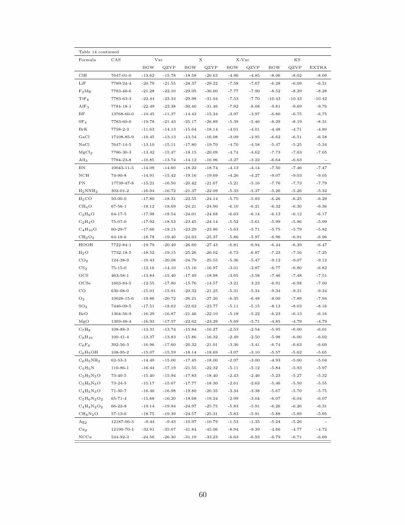
Table 14 continued

Formula CAS Vxc X X-Vxc KS

BGW QZVP BGW QZVP BGW QZVP BGW QZVP EXTRA

ClH 7647-01-0 -13.62 -15.78 -18.58 -20.63 -4.96 -4.85 -8.06 -8.02 -8.09

LiF 7789-24-4 -20.79 -21.55 -28.37 -29.22 -7.58 -7.67 -6.28 -6.09 -6.21

F2Mg 7783-40-6 -21.28 -22.10 -29.05 -30.00 -7.77 -7.90 -8.52 -8.29 -8.28

TiF4 7783-63-3 -22.44 -23.34 -29.98 -31.04 -7.53 -7.70 -10.43 -10.43 -10.42

AlF3 7784-18-1 -22.49 -23.38 -30.40 -31.46 -7.92 -8.08 -9.81 -9.69 -9.76

BF 13768-60-0 -10.45 -11.37 -14.42 -15.34 -3.97 -3.97 -6.80 -6.75 -6.75

SF4 7783-60-0 -19.78 -21.43 -25.17 -26.89 -5.39 -5.46 -8.29 -8.19 -8.31

BrK 7758-2-3 -11.63 -14.13 -15.64 -18.14 -4.01 -4.01 -4.48 -4.71 -4.80

GaCl 17108-85-9 -10.45 -13.13 -13.54 -16.08 -3.09 -2.95 -6.62 -6.51 -6.58

NaCl 7647-14-5 -13.10 -15.11 -17.80 -19.70 -4.70 -4.58 -5.47 -5.25 -5.34

MgCl2 7786-30-3 -13.42 -15.47 -18.15 -20.09 -4.74 -4.62 -7.73 -7.63 -7.65

AlI3 7784-23-8 -10.85 -13.74 -14.12 -16.96 -3.27 -3.22 -6.64 -6.63 -

BN 10043-11-5 -14.09 -14.60 -18.22 -18.74 -4.13 -4.14 -7.50 -7.46 -7.47

NCH 74-90-8 -14.91 -15.42 -19.16 -19.69 -4.26 -4.27 -9.07 -9.03 -9.05

PN 17739-47-8 -15.21 -16.50 -20.42 -21.67 -5.21 -5.16 -7.76 -7.73 -7.79

H2NNH2 302-01-2 -16.04 -16.72 -21.37 -22.09 -5.33 -5.37 -5.26 -5.26 -5.32

H2CO 50-00-0 -17.80 -18.31 -23.55 -24.14 -5.75 -5.83 -6.26 -6.25 -6.29

CH4O 67-56-1 -18.12 -18.69 -24.21 -24.90 -6.10 -6.21 -6.32 -6.30 -6.36

C2H6O 64-17-5 -17.98 -18.54 -24.01 -24.68 -6.03 -6.14 -6.13 -6.12 -6.17

C2H4O 75-07-0 -17.92 -18.53 -23.45 -24.14 -5.52 -5.61 -5.99 -5.96 -5.99

C4H10O 60-29-7 -17.66 -18.15 -23.29 -23.86 -5.63 -5.71 -5.75 -5.79 -5.82

CH2O2 64-18-6 -18.78 -19.40 -24.63 -25.37 -5.86 -5.97 -6.96 -6.91 -6.96

HOOH 7722-84-1 -19.79 -20.49 -26.60 -27.43 -6.81 -6.94 -6.44 -6.39 -6.47

H2O 7732-18-5 -18.52 -19.15 -25.26 -26.02 -6.73 -6.87 -7.23 -7.16 -7.25

CO2 124-38-9 -19.43 -20.08 -24.79 -25.55 -5.36 -5.47 -9.12 -9.07 -9.12

CS2 75-15-0 -12.16 -14.10 -15.16 -16.97 -3.01 -2.87 -6.77 -6.80 -6.82

OCS 463-58-1 -13.84 -15.40 -17.49 -18.98 -3.65 -3.58 -7.46 -7.48 -7.51

OCSe 1603-84-5 -12.55 -17.80 -15.76 -14.57 -3.21 3.23 -6.91 -6.98 -7.00

CO 630-08-0 -15.01 -15.91 -20.32 -21.25 -5.31 -5.34 -9.34 -9.31 -9.34

O3 10028-15-6 -19.86 -20.72 -26.21 -27.20 -6.35 -6.48 -8.00 -7.89 -7.94

SO2 7446-09-5 -17.51 -18.62 -22.62 -23.77 -5.11 -5.15 -8.13 -8.03 -8.16

BeO 1304-56-9 -16.29 -16.87 -21.46 -22.10 -5.18 -5.22 -6.23 -6.13 -6.16

MgO 1309-48-4 -16.93 -17.57 -22.62 -23.29 -5.69 -5.71 -4.85 -4.79 -4.79

C7H8 108-88-3 -13.31 -13.74 -15.84 -16.27 -2.53 -2.54 -5.95 -6.00 -6.01

C8H10 100-41-4 -13.37 -13.83 -15.86 -16.32 -2.49 -2.50 -5.98 -6.00 -6.02

C6F6 392-56-3 -16.96 -17.60 -20.32 -21.01 -3.36 -3.41 -6.74 -6.63 -6.69

C6H5OH 108-95-2 -15.07 -15.59 -18.14 -18.69 -3.07 -3.10 -5.57 -5.62 -5.65

C6H5NH2 62-53-3 -14.49 -15.00 -17.45 -18.00 -2.97 -3.00 -4.93 -5.00 -5.04

C5H5N 110-86-1 -16.44 -17.19 -21.55 -22.32 -5.11 -5.12 -5.84 -5.93 -5.97

C5H5N5O 73-40-5 -15.40 -15.94 -17.83 -18.40 -2.43 -2.46 -5.23 -5.27 -5.32

C5H5N5O 73-24-5 -15.17 -15.67 -17.77 -18.30 -2.61 -2.63 -5.46 -5.50 -5.55

C4H5N3O 71-30-7 -16.46 -16.98 -19.80 -20.35 -3.34 -3.38 -5.67 -5.70 -5.75

C5H6N2O2 65-71-4 -15.68 -16.20 -18.68 -19.24 -2.99 -3.04 -6.07 -6.04 -6.07

C4H4N2O2 66-22-8 -19.14 -19.84 -24.97 -25.75 -5.83 -5.91 -6.26 -6.26 -6.31

CH4N2O 57-13-6 -18.75 -19.39 -24.57 -25.31 -5.83 -5.91 -5.88 -5.89 -5.95

Ag2 12187-06-3 -9.44 -9.43 -10.97 -10.79 -1.53 -1.35 -5.24 -5.26 -

Cu2 12190-70-4 -32.91 -35.67 -41.84 -45.06 -8.94 -9.39 -4.66 -4.77 -4.72

NCCu 544-92-3 -24.56 -26.30 -31.19 -33.23 -6.63 -6.93 -6.79 -6.71 -6.69

60

Table 12: Threshold of the Gram-Schmidt orthogonalization (prodbas_acc)

1.d-5 1.d-6 1.d-7 1.d-8N2 -16.694478 -16.694478 -16.694478 -16.694477F2 -18.132832 -18.132834 -18.132837 -18.132838C2H6 -13.247344 -13.247344 -13.247344 -13.247344C3H6 -11.362216 -11.362215 -11.362215 -11.362215

Table 13: Threshold of the singular value decomposition (prodbas_threshold)

1.d-5 1.d-6 1.d-7 1.d-8N2 -16.694478 -16.694478 -16.694477 -16.694477F2 -18.132819 -18.132819 -18.132820 -18.132820C2H6 -13.247342 -13.247344 -13.247345 -13.247345C3H6 -11.362216 -11.362217 -11.362216 -11.362191

B Parameters plane wave calculations

B.1 pseudopotential parameters

B.2 Planewave cutoff energies

Table 16: Pseudopotential parameters for BerkeleyGW calculations.

Molecule Wavefunction cutoff (Ry)

Ethybenzene 80

Ozone 110

Boron nitride 110

Buthane 80

Tuloene 80

Phenol 100

Pyridine 100

Tetracarbon 80

Cesium dimer 50

Phosphorus dimer 50

Carbon dioxide 110

Helium atom 80

Beryllium monoxide 110

Magnesium monoxide 110

Borane 80

Hydrogen 90

Fluoroborane 90

Lithium dimer 50

Pentasilane 80

Disilane 80

Carbon oxyselenide 110

Gallium monochloride 60

Continues on next page

61

Table 16 continued

Molecule Wavefunction cutoff (Ry)

Phosphorus mononitride 110

Diborane 80

Arsenic dimer 50

Sodium dimer 50

Dipotassium 50

Dirubidium 50

Hydrazene 110

Hexafluorobenzene 90

Sodium tetramer 50

Sodium Hexamer 50

Carbon oxysulfide 110

Formaldehyde 110

Carbon tetraiodide 60

Cyclopentadiene 80

Carbon tetrabromide 60

Carbon tetrachloride 80

Urea 110

Vynil bromide 80

Vynil iodide 80

Ethoxy ehtane 100

Aniline 100

cyclooctatetraene 80

Carbon monoxide 110

Ethanol 100

Formic acid 110

Thymine 110

Uracil 110

Methanol 100

Cytosine 110

Benzene 80

Adenine 110

Guanine 110

Methane 90

Ethane 80

Ethylene 80

Acetylen 80

Hydrogen cyanide 110

Propane 80

Krypton atom 60

Neon atom 80

Argon atom 90

Sulfer dioxide 110

Vynil chloride 70

Vynil fluoride 90

Acetaldehyde 100

Carbon disulfide 70

Cyclopropane 80

Carbon tetrafluoride 90

Iodine 50

Lithium hydride 60

Hydrogen chloride 70

Sodium chloride 60

Hydrogen fluoride 90

Continues on next page

62

Table 16 continued

Molecule Wavefunction cutoff (Ry)

Amonia 110

Potassium hydride 60

Hydrogen peroxide 110

Bromine 60

Nitrogen 120

Water 110

Potassium bromide 70

Fluorine 90

chlorine 60

Germane 80

Hydrogen azide 120

Hydrogen sulfide 80

Magnesium fluoride 90

Sulfer tetrafluoride 90

Titanium fluoride 80

Aluminum trifluoride 90

Aluminum triiodide 50

Arsine 80

Magnesium chloride 60

Lithium fluoride 90

Phosphine 80

Silane 80

Copper dimer 350

Copper cyanide 350

Silver dimer 200

C Graphical solutions QPE

References

(1) Curtiss, L.; Raghavachari, K.; Trucks, G. W.; Pople, J. A. J. Chem. Phys 1991, 94,

7221.

(2) Curtiss, L. A.; Raghavachari, K.; Redfern, P. C.; Pople, J. A. J. Chem. Phys 1997,

106, 1063.

(3) Curtiss, L. A.; Redfern, P. C.; Raghavachari, K.; Pople, J. A. J. Chem. Phys 1998,

109, 42.

(4) GoÌĹricke, S., L.; Grimme PCCP 2011, 13,6670 .

63

Table 15: Pseudopotential parameters from the Espresso Library for BerkeleyGW calcula-tions. Nc the number of valence electrons, Rcuts the s-orbital cutoff (a.u.), Rcutp the p-orbitalcutoff (a.u.), Rcutd the d-orbital cutoff (a.u.)

Atom Nc Rcut-s(a.u.) Rcut-p (a.u.) Rcut-d (a.u.)H 1 0.50 N/A N/AHe 2 1.00 N/A N/ALi 1 2.45 2.45 N/ABe 2 2.10 2.10 N/AB 3 1.40 1.40 N/AC 4 1.30 1.30 N/AN 5 1.00 1.00 N/AO 6 1.10 1.10 N/AF 7 1.30 1.30 N/ANe 8 1.55 1.55 N/ANa 1 2.30 2.30 N/AMg 2 2.80 2.80 2.80Al 3 2.60 2.60 2.60Si 4 1.80 1.80 1.80P 5 1.95 1.95 1.95S 6 1.70 1.70 1.70Cl 7 1.75 1.75 1.75Ar 8 2.05 2.05 2.05K 1 3.51 3.76 3.76Ca 2 3.30 3.30 3.30Ga 3 2.05 2.45 2.75Ge 4 2.10 2.10 2.40As 5 2.10 2.10 2.10Se 6 1.90 1.90 1.90Br 7 1.95 1.95 1.95Kr 8 3.25 3.25 3.25Rb 1 3.82 3.82 3.72I 7 2.40 2.40 2.40Xe 8 3.25 3.25 3.25Cs 1 4.40 4.60 N/A

64

-14 -12 -10 -8-8

-6

-4

-2

0

2

4

6 BN

<HO

MO

|(E

)|HO

MO

> (e

V)

(eV)

TM -5 TM -3 BGW GPP AIMS 128 Pade AIMS 16 Pade AIMS 2 pole - KS + Vxc - x

-12 -10 -8 -6-10

-8

-6

-4

-2

0

2

4

6

8

10 BeO

<HO

MO

|(

)|HO

MO

> (e

V)

(eV)

TM -5 TM -3 BGW FF BGW GPP AIMS 128 Pade AIMS 16 Pade AIMS 2 pole - KS + Vxc - x

Figure 18: Comparison of the energy dependent correlation part of the self-energy Σc(ε)calculated with the three different codes using different procedures for Boron-nitride andBeryllium oxide. "TM -5" and "TM -3" indicate TURBOMOLE results calculated withimaginary shifts of 1e − 3 and 1e − 5 H respectively, "BGW-GPP" and "BGW-FF" in-dicate BerkeleyGW results using the Generalize Plasmon Pole model and Full Frequencyintegration method respectively, "AIMS-2P", "AIMS 128 Pade", and " AIMS 16 pade" indi-cate FHI-aims results using 2 Pole, 128 parameter Padé, and 16 parameter Padé analyticalcontinuation.

65

(5) S. Grimme, M. S.; Korth, M. J. Org. Chem. 2007, 72, 2118–2126.

(6) Goerigk, L.; Grimme, S. J. Chem. Theory Comput. 2010, 6, 107–126.

(7) Rezac, J.; Hobza, P. J. Chem. Theory Comput. 2011, 7, 685–689.

(8) Lejaeghere, K.; Van Speybroeck, V.; Van Oost, Guido,; Cottenier, S. Crit. Rev. Solid

State Mater. Sci. 39, 1.

(9) https://molmod.ugent.be/deltacodesdft.

(10) Perdew, J. P.; Burke, K.; Ernzerhof, M. Phys. Rev. Lett. 1996, 77, 3865.

(11) Hedin, L. Phys. Rev. 1965, 139, A796.

(12) Aulbur, W. G.; Jonsson, L.; Wilkins, J. W. Solid. State. Phys-adv. Res. Appl. 2000,

54, 1–218.

(13) Onida, G.; Reining, L.; Rubio, A. Rev. Mod. Phys. 2002, 74, 601–659.

(14) Rinke, P.; Qteish, A.; Neugebauer, J.; Freysoldt, C.; Scheffler, M. New J. of Phys.

2005, 7, 126.

(15) Ethridge, E. C.; Fry, J. L.; Zaider, M. Phys. Rev. B 1996, 53, 3662–3668.

(16) Ishii, S.; Ohno, K.; Kawazoe, Y.; Louie, S. G. Phys. Rev. B 2001, 63, 155104.

(17) Grossman, J. C.; Rohlfing, M.; Mitas, L.; Louie, S. G.; Cohen, M. L. Phys. Rev. Lett.

2001, 86, 472.

(18) Ishii, S.; Ohno, K.; Kawazoe, Y.; Louie, S. G. Phys. Rev. B 2002, 65, 245109.

(19) Ismail-Beigi, S.; Louie, S. G. Phys. Rev. Lett. 2003, 90, 076401.

(20) Pavlyukh, Y.; Hübner, W. Phys. Lett. A 2004, 327, 241.

(21) Tiago, M. L.; Chelikowsky, J. R. Phys. Rev. B 2006, 73, 205334.

66

(22) del Puerto, M. L.; Tiago, M. L.; Chelikowsky, J. R. Phys. Rev. Lett. 2006, 97, 096401.

(23) del Puerto, M. L.; Tiago, M. L.; Chelikowsky, J. R. Phys Rev. B 2008, 77, 045404.

(24) Ramos, L. E.; Paier, J.; Kresse, G.; Bechstedt, F. Phys Rev. B. 2008, 78, 195423.

(25) Noguchi, Y.; Ishii, S.; Ohno, K.; Sasaki, T. J. Chem. Phys. 2008, 129, 104104.

(26) Bruneval, F. Phys. Rev. Lett. 2009, 103, 176403.

(27) Tiago, M. L.; Idrobo, J. C.; Öğüt, S.; Jellinek, J.; Chelikowsky, J. R. Phys. Rev. B

2009, 79, 155419.

(28) Rostgaard, C.; Jacobsen, K. W.; Thygesen, K. S. Phys. Rev. B 2010, 81, 085103.

(29) Blase, X.; Attaccalite, C.; Olevano, V. Phys. Rev. B 2011, 83, 115103.

(30) Qian, X.; Umari, P.; Marzari, N. Phys. Rev. B 2011, 84, 075103.

(31) Refaely-Abramson, S.; Baer, R.; Kronik, L. Phys. Rev. B 2011, 84, 075144.

(32) Foerster, D.; Koval, P.; Sanchez-Portal, D. J. Chem. Phys. 2011, 135, 074105.

(33) Marom, N.; Ren, X.; Moussa, J. E.; Chelikowsky, J. R.; Kronik, L. Phys. Rev. B 2011,

84, 195143.

(34) Ke, S. Phys. Rev. B 2011, 84, 205415.

(35) Baumeier, B.; Andrienko, D.; Ma, Y.; Rohlfing, M. J. Chem. Theory Comput. 2012,

8, 997.

(36) Sharifzadeh, S.; Tamblyn, I.; Doak, P.; Darancet, P. T.; Neaton, J. B. Euro. Phys. J.

B 2012, 85, 323.

(37) Nguyen, H.-V.; Pham, T. A.; Rocca, D.; Galli, G. Phys. Rev. B 2012, 85, 081101.

(38) Caruso, F.; Rinke, P.; Ren, X.; Scheffler, M.; Rubio, A. Phys. Rev. B 2012, 86, 081102.

67

(39) Ren, X.; Rinke, P.; Blum, V.; Wieferink, J.; Tkatchenko, A.; Sanfilippo, A.; Reuter, K.;

Scheffler, M. New J. Phys. 2012, 14, 053020.

(40) Hübener, H.; Pérez-Osorio, M. A.; Ordejón, P.; Giustino, F. Phys. Rev. B 2012, 85,

245125.

(41) Körzdörfer, T.; Marom, N. Phys. Rev. B 2012, 86, 041110.

(42) Marom, N.; Caruso, F.; Ren, X.; Hofmann, O. T.; Körzdörfer, T.; Chelikowsky, J. R.;

Rubio, A.; Scheffler, M.; Rinke, P. Phys. Rev. B 2012, 86, 245127.

(43) Bruneval, F. The Journal of Chemical Physics 2012, 136, –.

(44) Pham, T. A.; Nguyen, H.-V.; Rocca, D.; Galli, G. Phys. Rev. B 2013, 87, 155148.

(45) Caruso, F.; Rinke, P.; Ren, X.; Rubio, A.; Scheffler, M. Phys. Rev. B 2013, 88, 075105.

(46) Bruneval, F.; Marques, M. A. L. J. Chem. Theory Comput. 2013, 9, 324.

(47) Faber, C.; Attaccalite, C.; Olevano, V.; Runge, E.; Blase, X. Phys. Rev. B 2011, 83,

115123.

(48) van Setten, M. J.; Weigend, F.; Evers, F. J. Chem. Theory Comput. 2013, 9, 232.

(49) Faber, C.; Boulanger, P.; Attaccalite, C.; Duchemin, I.; Blase, X. Philosophical Trans-

actions of the Royal Society A: Mathematical, Physical and Engineering Sciences

2014, 372 .

(50) Atalla, V.; Yoon, M.; Caruso, F.; Rinke, P.; Scheffler, M. Phys. Rev. B 2013, 88,

165122.

(51) Baumeier, B.; Rohlfing, M.; Andrienko, D. J. Chem. Theory Comput. 2014, 10, 3104–

3110.

(52) Hybertsen, M. S.; Louie, S. G. Phys. Rev. Lett. 1985, 55, 1418–1421.

68

(53) Hybertsen, M. S.; Louie, S. G. Phys. Rev. B 1986, 34, 5390.

(54) Godby, R. W.; Schlüter, M.; Sham, L. J. Phys. Rev. Lett. 1986, 56, 2415.

(55) Blum, V.; Gehrke, R.; Hanke, F.; Havu, P.; Havu, V.; Ren, X.; Reuter, K.; Scheffler, M.

Comput. Phys. Commun. 2009, 180, 2175–2196.

(56) Deslippe, J.; Samsonidze, G.; Strubbe, D. A.; Jain, M.; Cohen, M. L.; Louie, S. G.

Comput. Phys. Commun. 2012, 183, 1269.

(57) Holm, B.; von Barth, U. Physica Scripta 2004, 2004, 135.

(58) Fuchs, F.; Furthmüller, J.; Bechstedt, F.; Shishkin, M.; Kresse, G. Phys. Rev. B 2007,

76, 115109.

(59) Adler, S. L. Phys. Rev. 1962, 126, 413.

(60) Wiser, N. Phys. Rev. 1963, 129, 62.

(61) Freysoldt, C.; Eggert, P.; Rinke, P.; Schindlmayr, A.; Scheffler, M. Phys. Rev. B 2008,

77, 235428.

(62) Rozzi, C. A.; Varsano, D.; Marini, A.; Gross, E. K. U.; Rubio, A. Phys. Rev. B 2006,

73, 205119.

(63) Ismail-Beigi, S. Phys. Rev. B 2006, 73, 233103.

(64) Shishkin, M.; Kresse, G. Phys. Rev. B 2006, 74, 035101.

(65) Berger, A.; Reining, L.; Sottile, F. 2012, Phys. Rev. B, 085126.

(66) van Schilfgaarde, M.; Kotani, T.; Faleev, S. V. Phys. Rev. B 2006, 74, 245125.

(67) Arnaud, B.; Alouani, M. Phys. Rev. B 2000, 62, 4464.

(68) Torrent, M.; Jollet, F.; Bottin, F.; Zerah, G.; Gonze, X. Comput. Mat. Science 2008,

42, 337.

69

(69) Usuda, M.; Hamada, N.; Kotani, T.; van Schilfgaarde, M. Phys. Rev. B 2002, 66,

125101.

(70) Schindlmayr, A.; Friedrich, C.; Sasioglu, E.; Bluegel, S. Z. Phys. Chem. (Muenchen,

Ger.) 2010, 224, 357–368.

(71) Kutepov, A.; Haule, K.; Savrasov, S. Y.; Kotliar, G. Phys. Rev. B 2012, 85, 155129.

(72) Jiang, H.; Gómez-Abal, R. I.; Li, X.-Z.; Meisenbichler, C.; Ambrosch-Draxl, C.; Schef-

fler, M. Computer Physics Communications 2013, 184, 348 – 366.

(73) Kotani, T.; van Schilfgaarde, M. Solid State Commun. 2002, 121, 461.

(74) Fuchs, M.; Scheffler, M. Comput. Phys. Commun., Comput. Phys. Commun. 1999,

119, 67–98.

(75) Vanderbilt, D. Phys. Rev. B 1990, 41, 7892.

(76) Kleinman, L.; Bylander, D. M. Phys. Rev. Lett. 1982, 48, 1425–1428.

(77) Rappe, A. M.; Rabe, K. M.; Kaxiras, E.; Joannopoulos, J. D. Phys. Rev. B 1990, 41,

1227–1230.

(78) Oliveira, M.; Nogueira, F. Comput. Phys. Comm. 2008, 178, 524.

(79) Hamann, D. R. Phys. Rev. B 2013, 88, 085117.

(80) Rohlfing, M.; Krüger, P.; Pollmann, J. Phys. Rev. Lett. 1995, 75, 3489.

(81) Gómez-Abal, R.; Li, X.; Scheffler, M.; Ambrosch-Draxl, C. Phys. Rev. Lett. 2008,

101, 106404.

(82) Li, X.; Gomez-Abal, R.; Jiang, H.; Ambrosch-Draxl, C.; Scheffler, M. New J. Phys.

2012, 14, 023006.

70

(83) Liu, F.; Lin, L.; Vigil-Fowler, D.; Lischner, J.; Kemper, A. F.; Sharifzadeh, S.; da

Jornada, F. H.; Deslippe, J.; Yang, C.; Neaton, J. B.; Louie, S. G. J. Comput. Phys.

2015, 286, 1.

(84) Umari, P.; Stenuit, G.; Baroni, S. Phys. Rev. B 2009, 79, 201104.

(85) Berger, J. A.; Reining, L.; Sottile, F. Phys. Rev. B 2010, 82, 041103.

(86) private communication, Abinit calculation sternheimer approach, plane wave basis set.

(87) Hubener, H.; Giustino, F. J. Chem. Phys. 2014, 141, 044117.

(88) Sakuma, R.; Miyake, T.; Aryasetiawan, F. Phys. Rev. B 2009, 80, 235128.

(89) Guzzo, M.; Lani, G.; Sottile, F.; Romaniello, P.; Gatti, M.; Kas, J. J.; Rehr, J. J.;

Silly, M. G.; Sirotti, F.; Reining, L. Phys. Rev. Lett. 2011, 107, 166401.

(90) Lischner, J.; Vigil-Fowler, D.; Louie, S. G. Phys. Rev. Lett. 2013, 110, 146801.

(91) Hedin, L. J. Phys.: Condens. Matter 1999, 11, R489.

(92) Rinke, P.; Qteish, A.; Neugebauer, J.; Scheffler, M. phys. stat. sol. (b) 2008, 245, 929.

(93) Liu, F.; Lin, L.; Vigil-Fowler, D.; Lischner, J.; Kemper, A. F.; Sharifzadeh, S.; Jor-

nada, F. H.; Deslippe, J.; Yang, C.; Neaton, J. B.; Louie, S. G. LBNL Report 2014,

(94) Deslippe, J.; Samsonidze, G.; Jain, M.; Cohen, M. L.; Louie, S. G. Phys. Rev. B 2013,

87, 165124.

(95) Rieger, M. M.; Steinbeck, L.; White, I. D.; Rojas, H. N.; Godby, R. W. Comput. Phys.

Commun. 1999, 117, 211.

(96) Vidberg, H.; Serene, J. Journal of Low Temperature Physics 1977, 29, 179–192.

(97) Samsonidze, G.; Park, C.-H.; Kozinsky, B. Journal of Physics: Condensed Matter

2014, 26, 475501.

71

(98) Weigend, F.; Ahlrichs, R. Phys. Chem. Chem. Phys. 2005, 7, 3297.

(99) Eichkorn, K.; Treutler, O.; Oehm, H.; Haeser, M.; Ahlrichs, R. Chem. Phys. Lett.

1995, 240, 283.

(100) Weigend, F. Phys. Chem. Chem. Phys. 2006, 8, 1057.

(101) Giannozzi, P.; Baroni, S.; Bonini, N.; Calandra, M.; Car, R.; Cavazzoni, C.;

Ceresoli, D.; Chiarotti, G. L.; Cococcioni, M.; Dabo, I.; Corso, A. D.; de Giron-

coli, S.; Fabris, S.; Fratesi, G.; Gebauer, R.; Gerstmann, U.; Gougoussis, C.; Kokalj, A.;

Lazzeri, M.; Martin-Samos, L.; Marzari, N.; Mauri, F.; Mazzarello, R.; Paolini, S.;

Pasquarello, A.; Paulatto, L.; Sbraccia, C.; Scandolo, S.; Sclauzero, G.; Seitso-

nen, A. P.; Smogunov, A.; Umari, P.; Wentzcovitch, R. M. J. Physics: Cond. Matt.

2009, 21, 395502.

(102) Troullier, N.; Martins, J. L. Physical Review B 1991, 43, 1993–2006.

(103) www.qe-forge.org. 2013; http://www.qe-forge.org.

(104) Tamblyn, I.; Darancet, P.; Quek, S. Y.; Bonev, S. A.; Neaton, J. B. Phys. Rev. B

2011, 84, 201402.

(105) Goedecker, S.; Teter, M.; Hutter, J. Phys. Rev. B 1996, 54, 1703–1710.

(106) Hartwigsen, C.; Goedecker, S.; Hutter, J. Phys. Rev. B 1998, 58, 3641–3662.

(107) Lias, S. G.; Levin, R. D.; Kafafi, S. A. Ion Energetics Data in NIST Chemistry Web-

Book, NIST Standard Reference Database Number, 69th ed.; National Institute of

Standards and Technology, Gaithersburg MD, 20899 USA, 2003.

(108) Weast, R. C.; Astle, M. J. CRC Handbook of Chemistry and Physics, 92nd ed.; CRC

press, New York, 2011.

(109) Solov’yov, I. A.; Solov’yov, A. V.; Greiner, W. Phys. Rev. A 2002, 65, 053203.

72

(110) Chase, M. W.; Davies, C. A.; Downey, J. R.; Frurip, D. R.; McDonald, R. A.;

Syverud, A. N. J. Phys. Chem. Ref. Data 1985, 14, Suppl. 1.

(111) Hellwege, K. H.; Hellwege, A. M. Landolt-Bornstein: Group II: Atomic and Molecular

Physics Volume 7: Structure Data of Free Polyatomic Molecules ; Springer-Verlag,

Berlin, 1976.

(112) optimized 2d structure, using PBE functional and QZVP basis.

(113) Kummli, D. S.; Lobsiger, S.; Frey, H.-M.; Leutwyler, S.; Stanton, J. F. J. Phys. Chem.

A 2008, 112, 9134.

(114) Tolles, W. M.; Gwinn, W. D. J. Chem. Phys. 1962, 36, 1119.

(115) Coussan, B.; Perchard, Z. J. Phys. Chem. A 1998, 102, 5789.

(116) Kuchitsu(ed), K. Structure of Free Polyatomic Molecules - Basic Data; Springer,

Berlin, 1998.

(117) Godfrey, P. D.; Brown, R. D.; Hunter, A. N. Journal of Molecular Structure 1997,

413-414, 405 – 414.

(118) Simard, B.; Hackett, P. A. Chem. Phys. Lett. 2001, 186, 415–422.

(119) Aslund, N.; Barrow, R. F.; Richards, W. G.; Travis, O. N. Ark. Fys. 30, 171.

(120) Grossman, J. C.; Rohlfing, M.; Mitas, L.; Louie, S. G.; Cohen, M. L. Phys. Rev. Lett.

2001, 86, 472–475.

(121) Aryasetiawan, F.; Gunnarsson, O. Rep. Prog. Phys. 1998, 61, 237.

(122) Jain, M.; Deslippe, J.; Samsonidze, G.; Cohen, M.; Chelikowsky, J.; Louie, S. Phys.

Rev. B 2014, 90, 115148.

(123) Lischner, J.; Sharifzadeh, S.; Deslippe, J.; Neaton, J. B.; Louie, S. G. Phys. Rev. B

2014, 90, 115130.

73