Embed Size (px)
Citation preview
Title page for master’s thesis Faculty of Science and Technology
FACULTY OF SCIENCE AND TECHNOLOGY
MASTER’S THESIS
Study programme/specialisation:
Mechanical and Structural Engineering and Material ScienceSpecialization: Mechanical Engineering
Spring/ Autumn semester, 2020
Open / Confidential
Author: Adrian Otter Falch Günther Programme coordinator: Knut Erik Giljarhus Supervisor(s): Knut Erik Giljarhus Title of master’s thesis: Co-axial Propeller Configuration Optimization Credits: 30 Keywords:
UAV, Nordic Unnmanned,CFD, Co-Axial rotor setup, Low Reynolds, Axial Separation
Number of pages: 47
Stavanger, 29/06/2020 date/year

June 28, 2020
Abstract
The majority of research into Co-axial rotor setup involves same-sized pro-pellers. Different-sized propellers have received less attention. The combina-tion of low Reynolds number ( < 500 000) and different-sized propellers evenless.This thesis is looking into co-axial propeller interference with various ax-ial separation and effects concerning different-sized propellers in the co-axialsetup, while operating in a small scale. The studies were conducting us-ing Computational Fluid Dynamics simulations in the open-source softwareOpenFOAM.Using a larger sized lower propeller than upper propeller lowers the lowerpropeller efficiency loss by avoiding upper propeller slipstream affecting es-sential lift areas on the lower propeller. Using efficiency as a measure ofthrust per watts, the highest efficiency gain on lowest propeller was recordedusing a combination of a small and large propeller, respectively 28” and 32”diameter propeller. However, the highest overall efficiency was found usingboth upper and lower propeller as the largest (32”) propeller available, be-cause of the increase in efficiency of all propellers when reducing rotationalvelocity.The propeller axial separation study showed small variations on efficiencywhen the lower propeller is operating in the upper propeller’s slipstream.This is because of an increased efficiency of upper propeller while the ef-ficiency of lower propeller is decreased, with an increased axial separation.Only at very low axial separation values, the upper propeller had a signifi-cant loss of efficiency, which lead to an overall efficiency loss.
i
Preface
Finishing my Structural Engineering and Material Science degree at Uni-versity of Stavanger has because of Nordic Unmanned’s interesting problemproposal have been very enjoyable. First and foremost, I’d like to thank mysupervisor at UiS, Knut Erik Giljarhus, for patience and guidance through-out the process. I’d also like to thank the bachelor group consisting of StianRunestad Hidle and Vetle Byremo Ingebretsen, they have been providinginteresting discussions, and data to help guide and validate my simulations.And lastley Aboma Wagari Gebisa at UIS 3D Lab, aiding me with 3D scan-ning.
ii

Contents
Abstract i
Preface ii
1 Introduction 1
2 Theory 42.1 Aerodynamics . . . . . . . . . . . . . . . . . . . . . . . . . . . 4
2.1.1 Co-axial . . . . . . . . . . . . . . . . . . . . . . . . . . 62.2 Fluid Dynamics . . . . . . . . . . . . . . . . . . . . . . . . . . 6
2.2.1 Reynolds’s Number . . . . . . . . . . . . . . . . . . . . 72.2.2 Turbulence modelling . . . . . . . . . . . . . . . . . . . 82.2.3 Spalart Allmaras - SA . . . . . . . . . . . . . . . . . . 92.2.4 Laminar Separation Bubble . . . . . . . . . . . . . . . 10
2.3 Computational Fluid Dynamics . . . . . . . . . . . . . . . . . 112.3.1 Finite Volume Method . . . . . . . . . . . . . . . . . . 112.3.2 Discretiazation Schemes . . . . . . . . . . . . . . . . . 122.3.3 SIMPLE- and PIMPLE algorithm . . . . . . . . . . . . 122.3.4 Grid generation . . . . . . . . . . . . . . . . . . . . . . 132.3.5 OpenFOAM . . . . . . . . . . . . . . . . . . . . . . . . 14
3 STAAKER BG-200 153.1 System Description . . . . . . . . . . . . . . . . . . . . . . . . 15
3.1.1 Propeller Configuration . . . . . . . . . . . . . . . . . . 153.1.2 Flight Conditions . . . . . . . . . . . . . . . . . . . . . 18
4 Simulation of 2D Airfoil 204.1 Validation Case 2D . . . . . . . . . . . . . . . . . . . . . . . . 20
4.1.1 Computational Setup . . . . . . . . . . . . . . . . . . . 214.1.2 Results of the 2D airfoil simulations . . . . . . . . . . . 234.1.3 Discussion 2D Validation Case . . . . . . . . . . . . . . 28
iii
CONTENTS iv
4.1.4 Conclusion 2D Validation Case . . . . . . . . . . . . . 28
5 Simulation of 3D single- and co-axial rotor 305.1 3D - Single Rotor simulations . . . . . . . . . . . . . . . . . . 30
5.1.1 Computational Setup . . . . . . . . . . . . . . . . . . . 315.1.2 Results Single rotor Simulations . . . . . . . . . . . . . 32
5.2 3D - Co-Axial Rotor simulations . . . . . . . . . . . . . . . . . 375.2.1 Computational Setup . . . . . . . . . . . . . . . . . . 375.2.2 Results Co- axial simulations . . . . . . . . . . . . . . 375.2.3 Flight Endurance . . . . . . . . . . . . . . . . . . . . . 41
6 Conclusion 436.1 Computational Fluid Dynamics . . . . . . . . . . . . . . . . . 446.2 Further Work . . . . . . . . . . . . . . . . . . . . . . . . . . . 44
References 46
List of Figures
3.1 Staaker BG-200 . . . . . . . . . . . . . . . . . . . . . . . . . . 16
4.1 Grid . . . . . . . . . . . . . . . . . . . . . . . . . . . . . . . . 224.2 Surface Layer . . . . . . . . . . . . . . . . . . . . . . . . . . . 234.3 Coefficient of pressure over length along the wing . . . . . . . 234.4 Residuals vs Iterations . . . . . . . . . . . . . . . . . . . . . . 244.5 Pressure Along Chamber line . . . . . . . . . . . . . . . . . . 264.6 Residuals vs Iterations . . . . . . . . . . . . . . . . . . . . . . 264.7 Cp Along Chamber line, 4 AoA . . . . . . . . . . . . . . . . . 274.8 Cp Along Chamber line, 10 AoA . . . . . . . . . . . . . . . . . 27
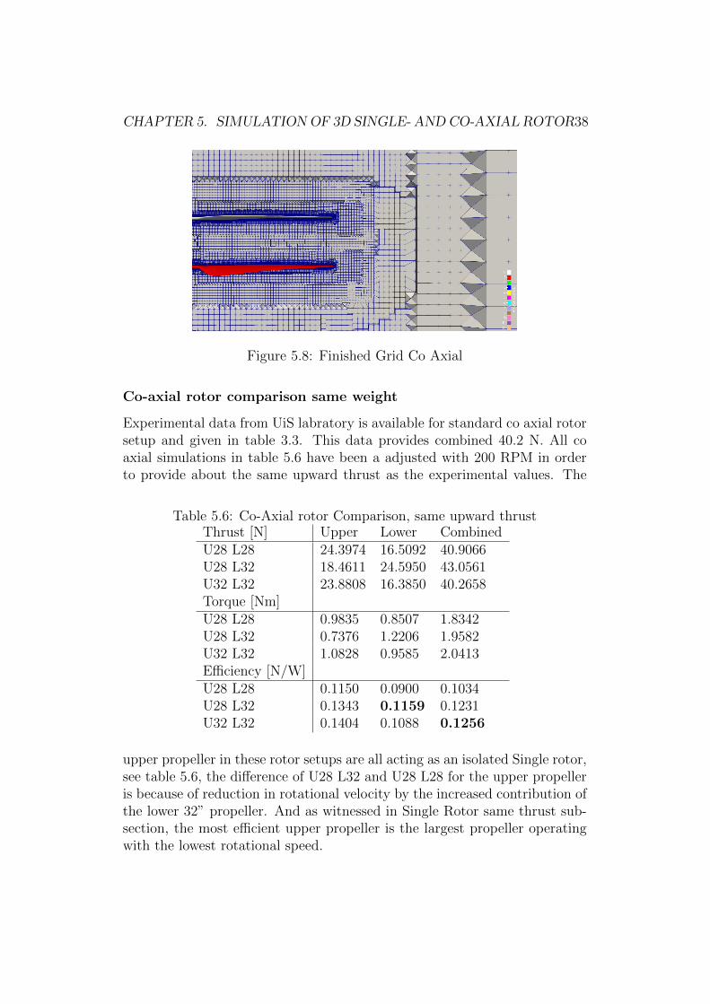
5.1 Grid refinement Level . . . . . . . . . . . . . . . . . . . . . . . 325.2 Surface Layer transition . . . . . . . . . . . . . . . . . . . . . 325.3 Single Rotor Thrust . . . . . . . . . . . . . . . . . . . . . . . . 335.4 Single Rotor Power . . . . . . . . . . . . . . . . . . . . . . . . 345.5 Efficiency Single Rotor . . . . . . . . . . . . . . . . . . . . . . 345.6 U 32” at 1700 RPM . . . . . . . . . . . . . . . . . . . . . . . . 365.7 U 32” at 2000 RPM . . . . . . . . . . . . . . . . . . . . . . . . 365.8 Finished Grid Co Axial . . . . . . . . . . . . . . . . . . . . . . 385.9 Lift Distribution . . . . . . . . . . . . . . . . . . . . . . . . . 395.10 Slipstream in a standard setup . . . . . . . . . . . . . . . . . . 395.11 Pressure Field of a standard setup . . . . . . . . . . . . . . . . 40
v

List of Tables
3.1 Propeller . . . . . . . . . . . . . . . . . . . . . . . . . . . . . . 163.2 3D modelled Propeller . . . . . . . . . . . . . . . . . . . . . . 173.3 Rotor Configuration - 40 N . . . . . . . . . . . . . . . . . . . . 183.4 Re across propeller blade . . . . . . . . . . . . . . . . . . . . . 19
4.1 Initial Grid Calculations . . . . . . . . . . . . . . . . . . . . . 224.2 Initial simulation . . . . . . . . . . . . . . . . . . . . . . . . . 244.3 Grid Independence . . . . . . . . . . . . . . . . . . . . . . . . 25
5.1 Initial Grid . . . . . . . . . . . . . . . . . . . . . . . . . . . . 315.2 Grid Refinement for Single 28” Propeller . . . . . . . . . . . . 335.3 3D model accuracy at 2000 RPM . . . . . . . . . . . . . . . . 355.4 Different Rotational Velocity . . . . . . . . . . . . . . . . . . . 355.5 Single Rotor Comparison, similar upward thrust . . . . . . . . 375.6 Co-Axial rotor Comparison, same upward thrust . . . . . . . . 385.7 Co-Axial rotor Comparison, Axial Separation . . . . . . . . . 41
vi
Nomenclature
Acronyms
BEMT Blade Element Momentum Theory
CAD Computer- Aided Design
CFD Computational Fluid Dynamics
LSB Laminar Separation Bubble
NACA National Advisory Committee for Aeronautics
NASA National Aeronautics and Space Administration
OpenFOAM Open source Field Operations and Manipulations
PISO Pressure Implicit with Splitting of Operator
RANS Reynolds-Average Navier Stokes
Re Reynolds Number
RPM Revolutions Per Minute
SA Spalart Allmaras
SIMPLE Semi-Implicit Method for Pressure Linked Equations
UAV Unmanned Aerial Vehicle
UiS University of Stavanger
Other symbols
ρ Density
A Surface Area
vii
NOMENCLATURE viii
Cd Drag Coefficient
Cl Lift Coefficient
FD Drag Force
FL Lift Force
g Gravitational Constant
∆ s First Layer Thickness
Γ Diffusion coefficient
κ Compressibility coefficient
µ Dynamic viscosity
∂ Partial derivative
φ Generic flux
τ Shear Stress
uτ Friction Velocity
c Chord length
div Divergence
divU Volumetric deformation
grad Gradient
k Turbulent kinetic energy
L Characteristic Length
l Chord width
r radius
U Mean velocity in x direction
u Instantaneous velocity in x direction
u’ Fluctuation velocity in x direction
V Mean velocity in y direction
NOMENCLATURE ix
v Instantaneous velocity in y direction
v’ Fluctuation velocity in y direction
W Mean velocity in z direction
w Instantaneous velocity in z direction
w’ Fluctuation velocity in z direction
y+ Dimensionless quantity
Introduction
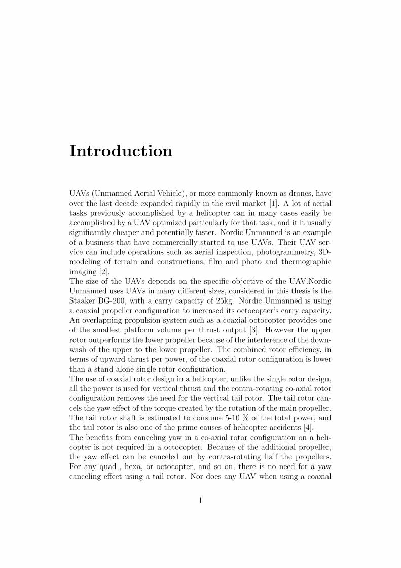
UAVs (Unmanned Aerial Vehicle), or more commonly known as drones, haveover the last decade expanded rapidly in the civil market [1]. A lot of aerialtasks previously accomplished by a helicopter can in many cases easily beaccomplished by a UAV optimized particularly for that task, and it it usuallysignificantly cheaper and potentially faster. Nordic Unmanned is an exampleof a business that have commercially started to use UAVs. Their UAV ser-vice can include operations such as aerial inspection, photogrammetry, 3D-modeling of terrain and constructions, film and photo and thermographicimaging [2].The size of the UAVs depends on the specific objective of the UAV.NordicUnmanned uses UAVs in many different sizes, considered in this thesis is theStaaker BG-200, with a carry capacity of 25kg. Nordic Unmanned is usinga coaxial propeller configuration to increased its octocopter’s carry capacity.An overlapping propulsion system such as a coaxial octocopter provides oneof the smallest platform volume per thrust output [3]. However the upperrotor outperforms the lower propeller because of the interference of the down-wash of the upper to the lower propeller. The combined rotor efficiency, interms of upward thrust per power, of the coaxial rotor configuration is lowerthan a stand-alone single rotor configuration.The use of coaxial rotor design in a helicopter, unlike the single rotor design,all the power is used for vertical thrust and the contra-rotating co-axial rotorconfiguration removes the need for the vertical tail rotor. The tail rotor can-cels the yaw effect of the torque created by the rotation of the main propeller.The tail rotor shaft is estimated to consume 5-10 % of the total power, andthe tail rotor is also one of the prime causes of helicopter accidents [4].The benefits from canceling yaw in a co-axial rotor configuration on a heli-copter is not required in a octocopter. Because of the additional propeller,the yaw effect can be canceled out by contra-rotating half the propellers.For any quad-, hexa, or octocopter, and so on, there is no need for a yawcanceling effect using a tail rotor. Nor does any UAV when using a coaxial
1
CHAPTER 1. INTRODUCTION 2
rotor setup.A small scale UAV operates within a lower Reynolds number airflow than amanned helicopter, which operate in a high Reynolds number airflow (Re >500,000). To accurately predict the performance of co axial rotors operatingin low Reynolds air flows is a challenging task. There is high complexity ofsingle propeller and co axial propeller airflow assessment, and serious prob-lems related to boundary separation and transitions have been encounteredat lower Re. Walker, at the Langley Research Center in Hampton studied aphenomenon called Laminar separation bubble, and found that the Eppler387 airfoil is dominated by laminar separation bubbles at Reynolds numbersbelow 200 000 [5].The turbulence model in this thesis is Spalart Allmaras. Spalart Allmarasis intended for fully turbulent high Reynolds number computations and isdemonstrated to not predict relaminarization [6].Looking at the combination of different sized propellers in a co-axial setup,Leishman and Anathan found that for a same sized propeller coaxial rotorsetup outside the region affected by the slipstream, the blade thrust gradientvalues of the lower propeller recovers to values that are consistent with theupper rotor [7]. Increasing the diameter of lower propeller compared to theupper propeller can therefore potentially diminish the efficiency loss of thelower propeller.Brazinskas et al looked at the co-axial separation and found that the axialseparation effects the rotors efficiency differently [3]. At an axial separationof 0.60 z/D, the upper rotor operates similar or even more efficient to theperformance of the single isolated rotor, while the lower rotor operates at thehighest efficiency loss at the same axial separation. The lower rotor operateswith the least efficiency loss around 0.05 z/D where the upper rotor has itshighest efficiency loss.Nordic Unmanned believes that one of the largest efficiency losses today isthe coaxial propeller configuration, and they seek to optimize their propellerconfiguration. The scope of this thesis is to optimize the co-axial propellerconfiguration of Staaker BG-200 to extend flight endurance. This will bedone using computational fluid dynamics, and by comparing the efficiency ofproposed co axial propeller configuration against the efficiency of a standardpropeller configuration currently used by Nordic Unmanned. Four differentpropellers commercially available is going to be tested, to determine whatconfiguration provides the highest value0s of upward thrust per power usage.This thesis will also look at a few selected axial separation distances and howthey effect the overall efficiency of the co-axial propeller configuration.The general theory behind the equations and methods used in this thesis willbe presented in chapter 2. Chapter 3 has case specific details and prepara-

CHAPTER 1. INTRODUCTION 3
tion of 3D models. This thesis is divided in terms of 2D- and 3D simulations,2D simulations are used as validation for turbulence model and proposedgrid structure. The 2D simulations are presented in chapter 4, while the3D simulations and the results of the co-axial CFD simulations will be pre-sented in chapter 5. Lastly, chapter 6 will conclude this thesis and presentrecommendation for further work.

Theory
This chapter will present the theory and governing equations in this thesis.Starting off with a simple introduction into aerodynamics and attemptingto highlight a few key differences and similarities between a normal airplanewing and a rotating propeller. Followed by basic fluid dynamics concepts andhow Reynolds Average Navier Stokes yields additional terms to the NavierStokes equations to model turbulent flow. Lastly, how Finite Volume Methodis used to to obtain an approximation of a solution to Reynold AveragedNavies Stoke partial differential equations.
2.1 Aerodynamics
In order to keep a object in air, lift generated by the plane needs to be largerthan the gravitational forces acting on the plane. And to move a planeforward, the forward thrust need to be larger than the drag forces acting onthe plane.Lift is generated when the shape of the object is forcing the streamlines tocurve around the object. In order to curve the streamlines its necessary witha pressure gradient, see equation 2.1.
∂p
∂r=ρU2
r, (2.1)
where r is the curve of the streamlines, U is the velocity. The pressure gra-dient acts as a centripetal force increasing the pressure-difference as velocityincreases or curve of the streamlines decreases. For an airfoil, assuming at-mospheric pressure far from the airfoil, this leads to a decreasing pressureon the upper surface of the airfoil and an increasing pressure on the lowersurface of the airfoil. This pressure difference gives a total aerodynamic forcewhich can be decomposed into lift- and drag force.Many objects can generate lift and its not always considered a wanted effect.
4
CHAPTER 2. THEORY 5
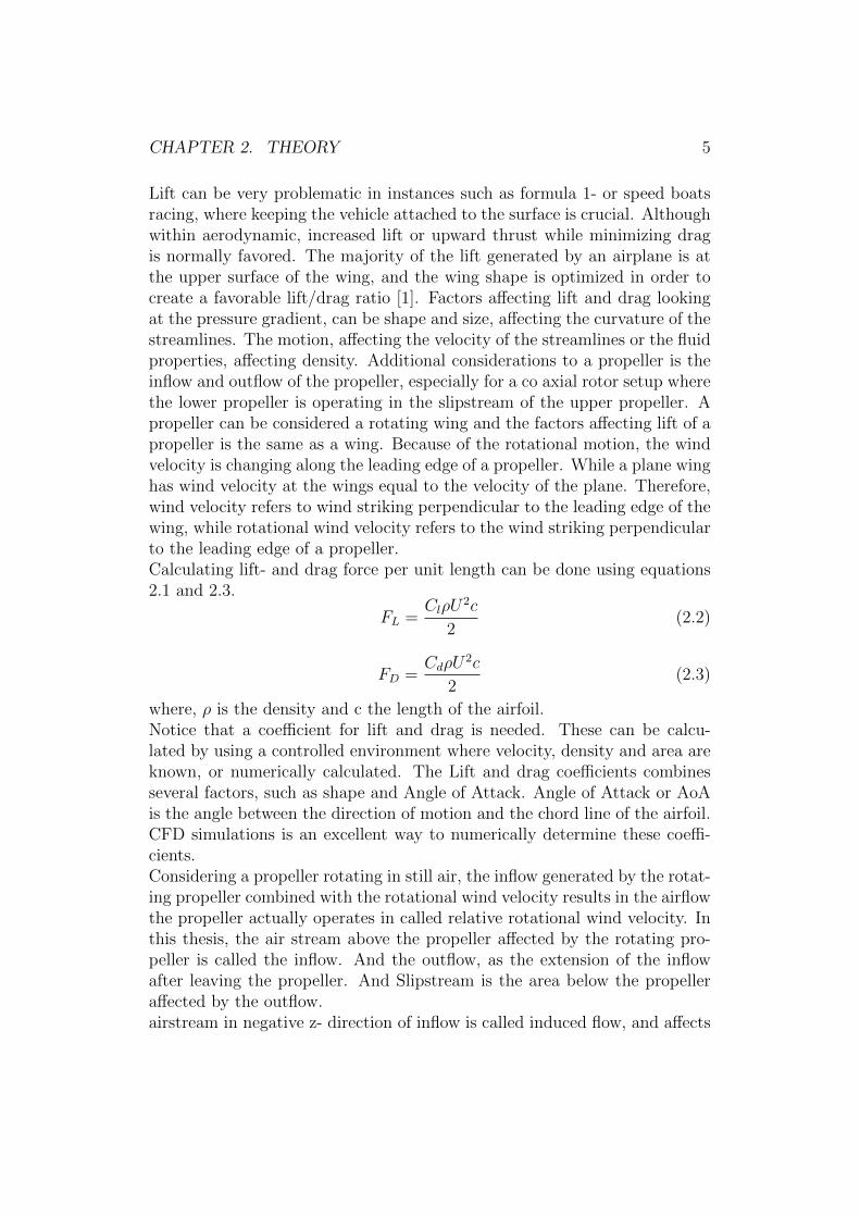
Lift can be very problematic in instances such as formula 1- or speed boatsracing, where keeping the vehicle attached to the surface is crucial. Althoughwithin aerodynamic, increased lift or upward thrust while minimizing dragis normally favored. The majority of the lift generated by an airplane is atthe upper surface of the wing, and the wing shape is optimized in order tocreate a favorable lift/drag ratio [1]. Factors affecting lift and drag lookingat the pressure gradient, can be shape and size, affecting the curvature of thestreamlines. The motion, affecting the velocity of the streamlines or the fluidproperties, affecting density. Additional considerations to a propeller is theinflow and outflow of the propeller, especially for a co axial rotor setup wherethe lower propeller is operating in the slipstream of the upper propeller. Apropeller can be considered a rotating wing and the factors affecting lift of apropeller is the same as a wing. Because of the rotational motion, the windvelocity is changing along the leading edge of a propeller. While a plane winghas wind velocity at the wings equal to the velocity of the plane. Therefore,wind velocity refers to wind striking perpendicular to the leading edge of thewing, while rotational wind velocity refers to the wind striking perpendicularto the leading edge of a propeller.Calculating lift- and drag force per unit length can be done using equations2.1 and 2.3.
FL =ClρU
2c
2(2.2)
FD =CdρU
2c
2(2.3)
where, ρ is the density and c the length of the airfoil.Notice that a coefficient for lift and drag is needed. These can be calcu-lated by using a controlled environment where velocity, density and area areknown, or numerically calculated. The Lift and drag coefficients combinesseveral factors, such as shape and Angle of Attack. Angle of Attack or AoAis the angle between the direction of motion and the chord line of the airfoil.CFD simulations is an excellent way to numerically determine these coeffi-cients.Considering a propeller rotating in still air, the inflow generated by the rotat-ing propeller combined with the rotational wind velocity results in the airflowthe propeller actually operates in called relative rotational wind velocity. Inthis thesis, the air stream above the propeller affected by the rotating pro-peller is called the inflow. And the outflow, as the extension of the inflowafter leaving the propeller. And Slipstream is the area below the propelleraffected by the outflow.airstream in negative z- direction of inflow is called induced flow, and affects
CHAPTER 2. THEORY 6
the direction of motion. AoA is effected by inflow by increased velocity ofinduced flow leads to a declined relative rotational wind direction, normallydecreases the AoA. since AoA and the lift closely related,an increase of themagnitude of induced flow would lead to a decrease in lift because of the newrelative rotational wind orientation decreased the AoA.
2.1.1 Co-axial
Co- axial propeller configuration is a configuration where a pair of propelleris operating, one above the other. Both propeller generate lift in the sameway as an isolated propeller, but the resultant airflow is different dependenton interference between the lower and upper propeller. As mentioned in theintroduction, co-axial propeller setup is beneficial for canceling the torque,normally created by a single rotor setup and removing the need for a verticaltail rotor. In addition to the inflow generated by the lower propeller in acoaxial setup, the lower propeller is also operating in the slipstream of theUpper propeller.
2.2 Fluid Dynamics
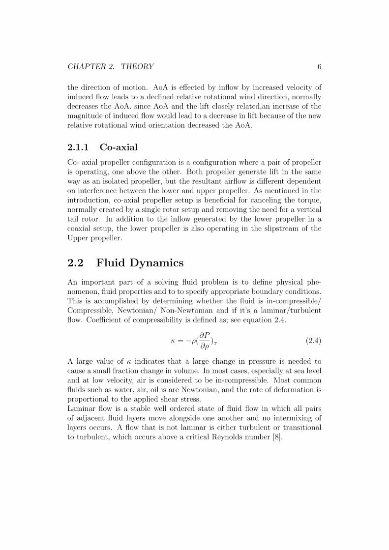
An important part of a solving fluid problem is to define physical phe-nomenon, fluid properties and to to specify appropriate boundary conditions.This is accomplished by determining whether the fluid is in-compressible/Compressible, Newtonian/ Non-Newtonian and if it’s a laminar/turbulentflow. Coefficient of compressibility is defined as; see equation 2.4.
κ = −ρ(∂P
∂ρ)T
(2.4)
A large value of κ indicates that a large change in pressure is needed tocause a small fraction change in volume. In most cases, especially at sea leveland at low velocity, air is considered to be in-compressible. Most commonfluids such as water, air, oil is are Newtonian, and the rate of deformation isproportional to the applied shear stress.Laminar flow is a stable well ordered state of fluid flow in which all pairsof adjacent fluid layers move alongside one another and no intermixing oflayers occurs. A flow that is not laminar is either turbulent or transitionalto turbulent, which occurs above a critical Reynolds number [8].
CHAPTER 2. THEORY 7
2.2.1 Reynolds’s Number
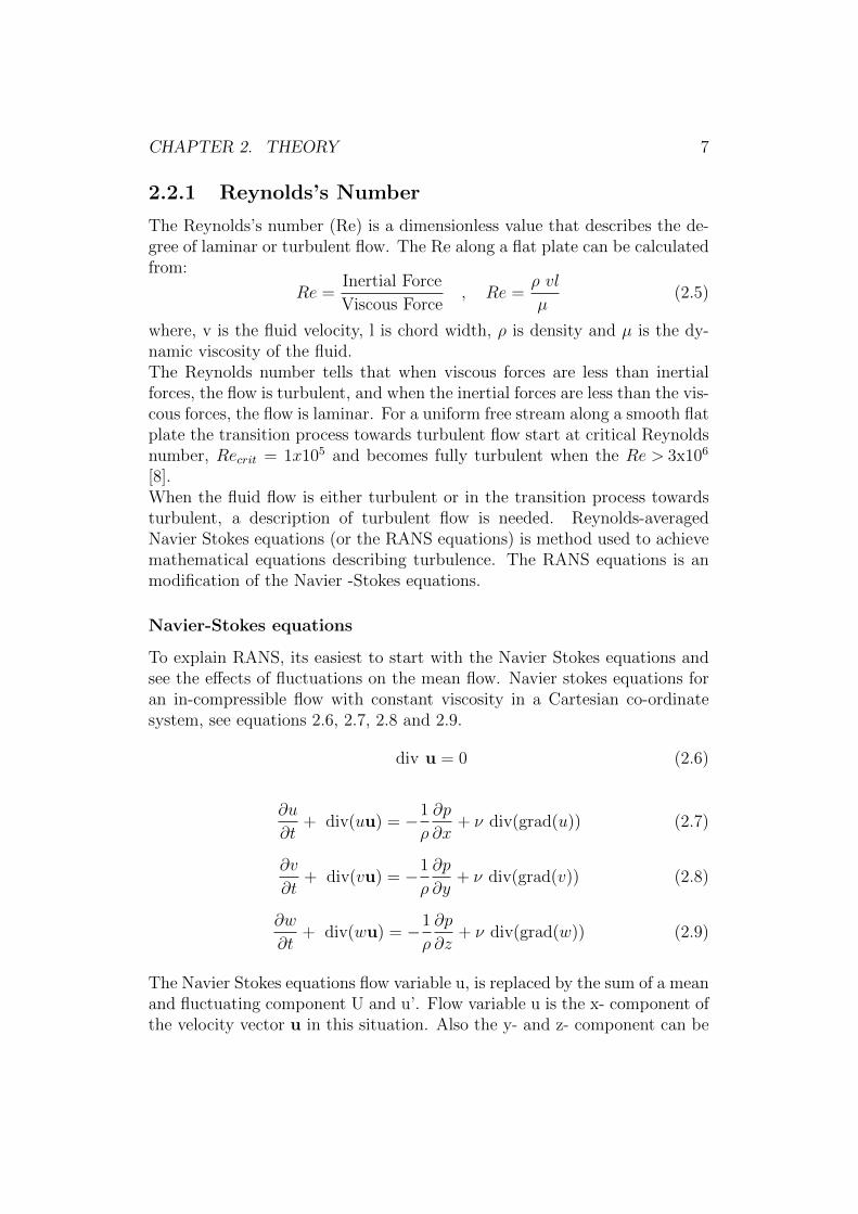
The Reynolds’s number (Re) is a dimensionless value that describes the de-gree of laminar or turbulent flow. The Re along a flat plate can be calculatedfrom:
Re =Inertial Force
Viscous Force, Re =
ρ vl
µ(2.5)
where, v is the fluid velocity, l is chord width, ρ is density and µ is the dy-namic viscosity of the fluid.The Reynolds number tells that when viscous forces are less than inertialforces, the flow is turbulent, and when the inertial forces are less than the vis-cous forces, the flow is laminar. For a uniform free stream along a smooth flatplate the transition process towards turbulent flow start at critical Reynoldsnumber, Recrit = 1x10⁵ and becomes fully turbulent when the Re > 3x10⁶
[8].When the fluid flow is either turbulent or in the transition process towardsturbulent, a description of turbulent flow is needed. Reynolds-averagedNavier Stokes equations (or the RANS equations) is method used to achievemathematical equations describing turbulence. The RANS equations is anmodification of the Navier -Stokes equations.
Navier-Stokes equations
To explain RANS, its easiest to start with the Navier Stokes equations andsee the effects of fluctuations on the mean flow. Navier stokes equations foran in-compressible flow with constant viscosity in a Cartesian co-ordinatesystem, see equations 2.6, 2.7, 2.8 and 2.9.
div u = 0 (2.6)
∂u
∂t+ div(uu) = −1
ρ
∂p
∂x+ ν div(grad(u)) (2.7)
∂v
∂t+ div(vu) = −1
ρ
∂p
∂y+ ν div(grad(v)) (2.8)
∂w
∂t+ div(wu) = −1
ρ
∂p
∂z+ ν div(grad(w)) (2.9)
The Navier Stokes equations flow variable u, is replaced by the sum of a meanand fluctuating component U and u’. Flow variable u is the x- component ofthe velocity vector u in this situation. Also the y- and z- component can be
CHAPTER 2. THEORY 8
replaced, thus table 2.2.1.
u = U + u’ u = U + u’ v = V + v’ w = W + w’ p = P + p’
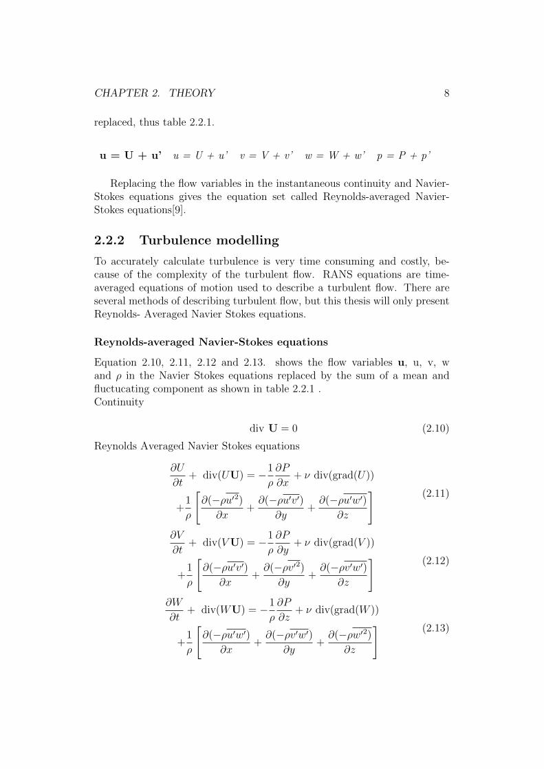
Replacing the flow variables in the instantaneous continuity and Navier-Stokes equations gives the equation set called Reynolds-averaged Navier-Stokes equations[9].
2.2.2 Turbulence modelling
To accurately calculate turbulence is very time consuming and costly, be-cause of the complexity of the turbulent flow. RANS equations are time-averaged equations of motion used to describe a turbulent flow. There areseveral methods of describing turbulent flow, but this thesis will only presentReynolds- Averaged Navier Stokes equations.
Reynolds-averaged Navier-Stokes equations
Equation 2.10, 2.11, 2.12 and 2.13. shows the flow variables u, u, v, wand ρ in the Navier Stokes equations replaced by the sum of a mean andfluctucating component as shown in table 2.2.1 .Continuity
div U = 0 (2.10)
Reynolds Averaged Navier Stokes equations
∂U
∂t+ div(UU) = −1
ρ
∂P
∂x+ ν div(grad(U))
+1
ρ
[∂(−ρu′2)
∂x+∂(−ρu′v′)
∂y+∂(−ρu′w′)
∂z
] (2.11)
∂V
∂t+ div(VU) = −1
ρ
∂P
∂y+ ν div(grad(V ))
+1
ρ
[∂(−ρu′v′)
∂x+∂(−ρv′2)
∂y+∂(−ρv′w′)
∂z
] (2.12)
∂W
∂t+ div(WU) = −1
ρ
∂P
∂z+ ν div(grad(W ))
+1
ρ
[∂(−ρu′w′)
∂x+∂(−ρv′w′)
∂y+∂(−ρw′2)
∂z
] (2.13)
CHAPTER 2. THEORY 9
Comparing the Reynolds-average Navier Stokes equations with the NavierStokes equations, on the right hand side there is additional terms. Thesenew terms involve products of fluctuating velocities and are associated withconvective momentum transfer due to turbulent eddies. They result from sixadditional turbulent stresses and are called the Reynolds stresses[9].
Reynolds stresses
Three normal stresses
τxx = −ρu′2 τyy = −ρv′2 τzz = −ρw′2 (2.14)
and three shear stresses.
τxy = τyx = −ρu′v′ τxz = τzx − ρu′w′ τyz = τzy − ρv′w′ (2.15)
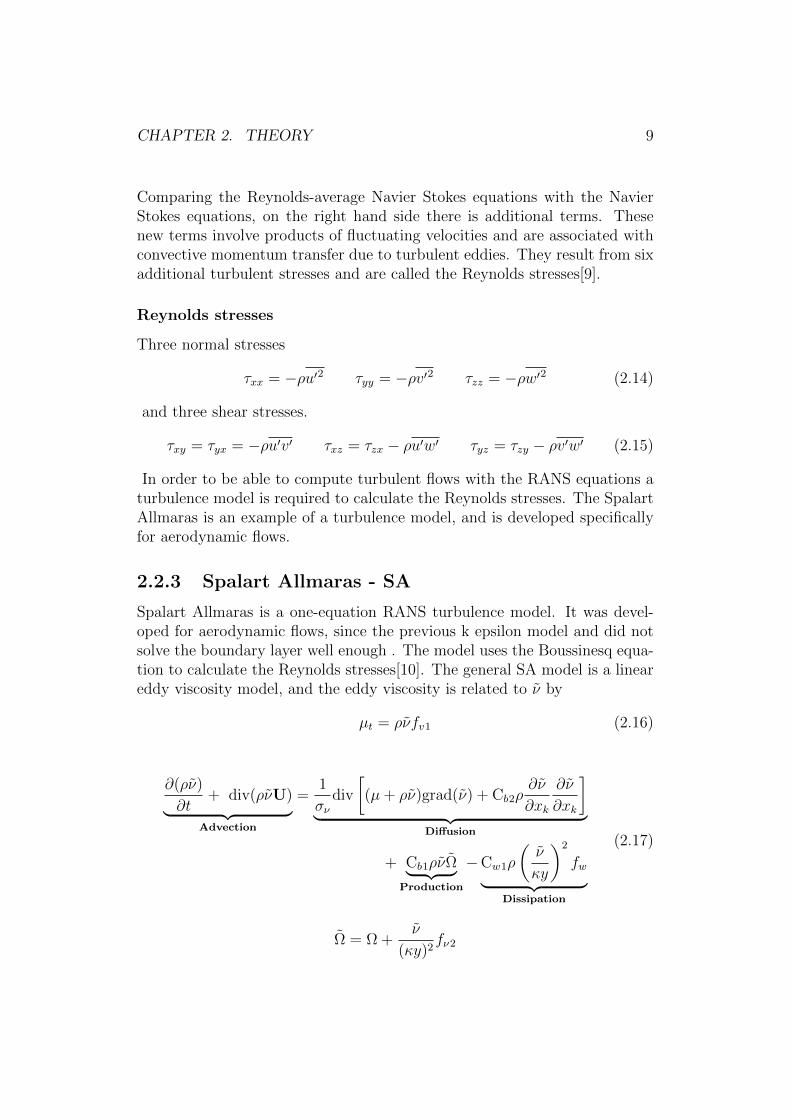
In order to be able to compute turbulent flows with the RANS equations aturbulence model is required to calculate the Reynolds stresses. The SpalartAllmaras is an example of a turbulence model, and is developed specificallyfor aerodynamic flows.
2.2.3 Spalart Allmaras - SA
Spalart Allmaras is a one-equation RANS turbulence model. It was devel-oped for aerodynamic flows, since the previous k epsilon model and did notsolve the boundary layer well enough . The model uses the Boussinesq equa-tion to calculate the Reynolds stresses[10]. The general SA model is a lineareddy viscosity model, and the eddy viscosity is related to ν by
µt = ρνfv1 (2.16)
∂(ρν)
∂t+ div(ρνU)︸ ︷︷ ︸
Advection
=1
σνdiv
[(µ+ ρν)grad(ν) + Cb2ρ
∂ν
∂xk
∂ν
∂xk
]︸ ︷︷ ︸
Diffusion
+ Cb1ρνΩ︸ ︷︷ ︸Production
−Cw1ρ
(ν
κy
)2
fw︸ ︷︷ ︸Dissipation
(2.17)
Ω = Ω +ν
(κy)2fν2
CHAPTER 2. THEORY 10
whereΩ =
√2ΩijΩij = mean vorticity
and
Ωij =1
2
(∂Ui∂xj
− ∂Uj∂xi
)= mean vorticity tensor
The functions
fv1 = fv1(ν
ν)
,
fv2 = fv2(ν
ν)
and
fw = fw(ν
Ωκ2y2)
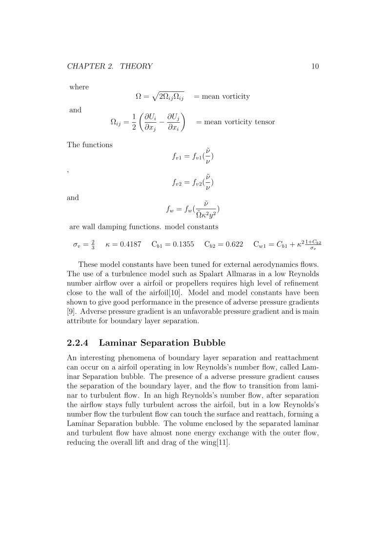
are wall damping functions. model constants
σv = 23
κ = 0.4187 Cb1 = 0.1355 Cb2 = 0.622 Cw1 = Cb1 + κ2 1+Cb2
σv
These model constants have been tuned for external aerodynamics flows.The use of a turbulence model such as Spalart Allmaras in a low Reynoldsnumber airflow over a airfoil or propellers requires high level of refinementclose to the wall of the airfoil[10]. Model and model constants have beenshown to give good performance in the presence of adverse pressure gradients[9]. Adverse pressure gradient is an unfavorable pressure gradient and is mainattribute for boundary layer separation.
2.2.4 Laminar Separation Bubble
An interesting phenomena of boundary layer separation and reattachmentcan occur on a airfoil operating in low Reynolds’s number flow, called Lam-inar Separation bubble. The presence of a adverse pressure gradient causesthe separation of the boundary layer, and the flow to transition from lami-nar to turbulent flow. In an high Reynolds’s number flow, after separationthe airflow stays fully turbulent across the airfoil, but in a low Reynolds’snumber flow the turbulent flow can touch the surface and reattach, forming aLaminar Separation bubble. The volume enclosed by the separated laminarand turbulent flow have almost none energy exchange with the outer flow,reducing the overall lift and drag of the wing[11].
CHAPTER 2. THEORY 11
2.3 Computational Fluid Dynamics
Computational Fluid Dynamics or CFD, is a computer-based simulations andanalysis of a systems involving fluid flow, by the means of computer-basedsimulations. An example of one of the industries utilizing this techniqueis industries concerning aerodynamics of aircraft and vehicles. Formula 1wanting to reducing drag or/and increase downforce (reversed lift, spoiler),commercial airplanes minimizing costs or the military increasing flight lengthof their missiles. Some of the benefits using CFD is substantially reduction ofcosts of new design, study systems without risk concerning hazardous condi-tion or pushing systems beyond their capacity without the costs of accidentsscenarios. Most commercial CFD packages contain three main elements,pre- processor, a solver and post processing. The pre –processor consistsof defining the computational domain, creating a grid with a satisfactorygrid quality, specify fluid properties and boundary conditions. Finite volumemethod is a numerical solution technique used in the most well establishedCFD codes and used as the solver element of this thesis. The last element ofCFD packages is post processing and used to presents the results from thesimulations [9].
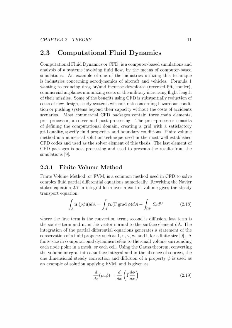
2.3.1 Finite Volume Method
Finite Volume Method, or FVM, is a common method used in CFD to solvecomplex fluid partial differential equations numerically. Rewriting the Navierstokes equation 2.7 in integral form over a control volume gives the steadytransport equation:∫
A
n.(ρφu)dA =
∫A
n.(Γ grad φ)dA+
∫CV
SφdV (2.18)
where the first term is the convection term, second is diffusion, last term isthe source term and n. is the vector normal to the surface element dA. Theintegration of the partial differential equations generates a statement of theconservation of a fluid property such as 1, u, v, w, and i, for a finite size [9] . Afinite size in computational dynamics refers to the small volume surroundingeach node point in a mesh, or each cell. Using the Gauss theorem, convertingthe volume integral into a surface integral and in the absence of sources, theone dimensional steady convection and diffusion of a property φ is used asan example of solution applying FVM, and is given as:
d
dx(ρuφ) =
d
dx
(Γdφ
dx
)(2.19)
CHAPTER 2. THEORY 12
which must satisfy continuity, so d(ρu)dx
= 0. Integrating the transport equa-tion focused on a general node P; with neighbouring control volume faces wand e:
(ρuAφ)e − (ρuAφ)w =
(ΓA
dφ
dx
)e
−(
ΓAdφ
dx
)w
(2.20)
With continuity integrated as, (ρuA)e − (ρuA)w = 0, let variable F and Drepresent the convective mass flux per unit area and diffusion conductanceat cell faces. The integrated convection - diffusion equation can be rewrittenas:
Feφe − Fwφw = De(φE − φP ) −Dw(φP − φW ) (2.21)
And integrated continuity equation as Fe−Fw = 0. Discretiazation schemescan be used in order to calculate the transported property φ at the e and wfaces[9].
2.3.2 Discretiazation Schemes
Utilizing FVM as method for solving CFD simulations, requires discretisationschemes to calculate the transport properties φe and φw. The most commondiscretisation schemes, and used in this thesis, is the Central differencingscheme and Upwind differencing scheme.Central differencing scheme seems to yield accurate results when the F/Dratio is low, and the convection- diffusen problems takes the same generalform as for pure diffusion. Central differencing schemes are usually an ef-fective choice of gradient scheme. Upwind Differencing schemes is beneficialwhen the flow becomes strongly convective because the direction is takeninto account [12].
2.3.3 SIMPLE- and PIMPLE algorithm
The most popular solution algorithms for pressure and velocity calculationsis SIMPLE, which is an iterative procedure for calculation of pressure andvelocity fields. Suited for steady state, incompressible and turbulent flow.SIMPLE stands for Semi- Implicit Method for Pressure Linked Equations andis basically a guess and correct solver, and starting from an initial pressurefield guess p*. Then solving the discretised momentum equations to com-pute the intermediate velocity field, solving the pressure correction equations,correcting the pressure and velocities, solving all other discretised transportequations and finally see if the pressure-, and velocity corrections will all be
CHAPTER 2. THEORY 13
zero in a converged solution. If not, the Simple Algorithm set p* = p, u* =u, v* = v and φ* = φ and repeat until the solution has converged or reachedpreferred tolerance [9]. In this thesis, a dynamic mesh will be introduced inorder to simulate rotating propellers. Since Simple is a steady state solver,a transient solver must be introduced.PIMPLE algorithm is a combination of PISO and SIMPLE, where PISO(Pressure Implicit with Splitting of Operators) has a further corrector stepto SIMPLE. PIMPLE is a transient solver for incompressible, turbulent flowof a Newtonian fluid, suited for a moving mesh. Pimple solves the equationof momentum equal to the one in SIMPLE, except that time differential isused for calculation sphere. Can be thought of as a SIMPLE solver for eachtime step, and once converged, the solver will move on to the next time step.
2.3.4 Grid generation
Grid generation is a major part of the pre processsor element of most CFDpackages. The accuracy of a CFD solution is hugely affected by the numberof cells in the grid. A finer grid tends to provide more accurate solution, butat an increasingly computational cost. Optimal meshes are finer in areas oflarge variations and coarser in areas of little change. Presently it’s up to theCFD user to design a grid that is suitable for the given case [9].The far field boundaries are fairly easy to determine in a external flow field,but the increased cell refinement around model surface can be more difficultto determine. Y+ is a none dimensional distance representing the distancefrom a model surface to the first cell node, takes into account the fluid motion,properties, geometry and friction of the wall, and can be used to determinethe highest level of refinement needed in a mesh. In order to generate anoptimal mesh, using the first layer height calculated using an appropriatey+ value and smooth transition into the background mesh can provide a lowcomputational mesh still providing high accuracy simulations.
Surface Layer
In order to calculate y+ at a flat plate, use Reynolds’s Number calculatedfrom equation 2.5 to determine the friction coefficient at the wall. For asmooth surface, use equation 2.22.
Cf =0.026
Re1/7x
(2.22)
CHAPTER 2. THEORY 14
Knowing the friction coefficient, equation 2.23 is used to calculate the wallshear stress, where U∞ is the free air stream velocity.
τwall =CfρU
2∞
2(2.23)
Using the wall shear stress, equation 2.24 is used to calculate the frictionvelocity used in equation 2.25. Use equation 2.25 to calculate the first layerheight using an appropriate y+ value.
Ufric =
√τwallρ
(2.24)
∆s =y+µ
Ufricρ(2.25)
In aerodynamics and airfoils operating in transitional or turbulent flow, theoccurrence of adverse pressure gradients, requires the first layer height tobe within the viscous sub-layer. A reasonable y+ value using the SpalartAllmaras turbulence model is y+ of less than 1 [13].
2.3.5 OpenFOAM
OpenFOAM stand for Open source Field Operation And Manipulation. Open-FOAM being a Open source CFD toolkit allows the user to freely use andmodify a high-end CFD code. OpenFOAM is operated from the terminalwindow and written in C++.With the absence of an integrated graphical user interface, OpenFOAM is afolder based toolkit and consist of three main directories, constant, systemand 0 [14].
STAAKER BG-200
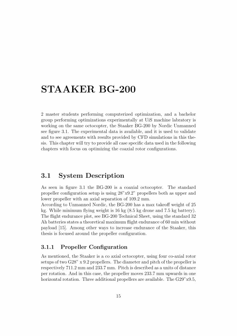
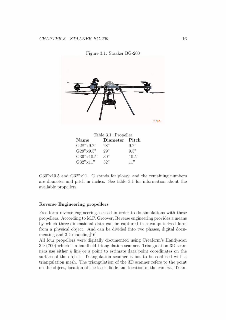
2 master students performing computerized optimization, and a bachelorgroup performing optimizations experimentally at UiS machine labratory isworking on the same octocopter, the Staaker BG-200 by Nordic Unmannedsee figure 3.1. The experimental data is available, and it is used to validateand to see agreements with results provided by CFD simulations in this the-sis. This chapter will try to provide all case specific data used in the followingchapters with focus on optimizing the coaxial rotor configurations.
3.1 System Description
As seen in figure 3.1 the BG-200 is a coaxial octocopter. The standardpropeller configuration setup is using 28”x9.2” propellers both as upper andlower propeller with an axial separation of 109.2 mm.According to Unmanned Nordic, the BG-200 has a max takeoff weight of 25kg. While minimum flying weight is 16 kg (8.5 kg drone and 7.5 kg battery).The flight endurance plot, see BG-200 Technical Sheet, using the standard 32Ah batteries states a theoretical maximum flight endurance of 60 min withoutpayload [15]. Among other ways to increase endurance of the Staaker, thisthesis is focused around the propeller configuration.
3.1.1 Propeller Configuration
As mentioned, the Staaker is a co axial octocopter, using four co-axial rotorsetups of two G28” x 9.2 propellers. The diameter and pitch of the propeller isrespectively 711.2 mm and 233.7 mm. Pitch is described as a units of distanceper rotation. And in this case, the propeller moves 233.7 mm upwards in onehorizontal rotation. Three additional propellers are available. The G29”x9.5,
15
CHAPTER 3. STAAKER BG-200 16
Figure 3.1: Staaker BG-200
Table 3.1: PropellerName Diameter PitchG28”x9.2” 28” 9.2”G29”x9.5” 29” 9.5”G30”x10.5” 30” 10.5”G32”x11” 32” 11”
G30”x10.5 and G32”x11. G stands for glossy, and the remaining numbersare diameter and pitch in inches. See table 3.1 for information about theavailable propellers.
Reverse Engineering propellers
Free form reverse engineering is used in order to do simulations with thesepropellers. According to M.P. Groover, Reverse engineering provides a meansby which three-dimensional data can be captured in a computerized formfrom a physical object. And can be divided into two phases, digital docu-menting and 3D modeling[16].All four propellers were digitally documented using Creaform’s Handyscan3D (700) which is a handheld triangulation scanner. Triangulation 3D scan-ners use either a line or a point to estimate data point coordinates on thesurface of the object. Triangulation scanner is not to be confused with atriangulation mesh. The triangulation of the 3D scanner refers to the pointon the object, location of the laser diode and location of the camera. Trian-
CHAPTER 3. STAAKER BG-200 17
Table 3.2: 3D modelled PropellerName filetype Diameter Pitch AoAG28 9.2 CW .stl 710 mm 234 mm 11,9
G28 9.2 CCW .stl 710 mm 234 mm 11,9
G29 9.5 CW .stl 734 mm 241 mm 11,9
G29 9.5 CCW .stl 734 mm 241 mm 11,9
G30 10.5 CW .stl 762 mm 267 mm 12,3
G30 10.5 CCW .stl 762 mm 267 mm 12,3
G32 11 CW .stl 816 mm 279 mm 12,7
G32 11 CCW .stl 816 mm 279 mm 12,7
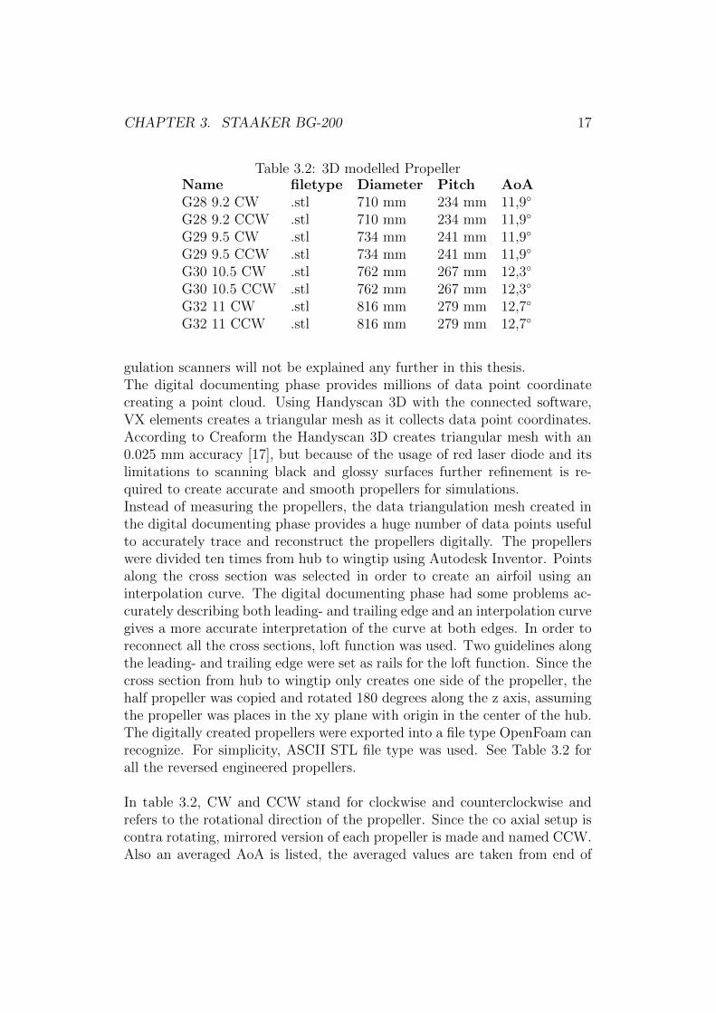
gulation scanners will not be explained any further in this thesis.The digital documenting phase provides millions of data point coordinatecreating a point cloud. Using Handyscan 3D with the connected software,VX elements creates a triangular mesh as it collects data point coordinates.According to Creaform the Handyscan 3D creates triangular mesh with an0.025 mm accuracy [17], but because of the usage of red laser diode and itslimitations to scanning black and glossy surfaces further refinement is re-quired to create accurate and smooth propellers for simulations.Instead of measuring the propellers, the data triangulation mesh created inthe digital documenting phase provides a huge number of data points usefulto accurately trace and reconstruct the propellers digitally. The propellerswere divided ten times from hub to wingtip using Autodesk Inventor. Pointsalong the cross section was selected in order to create an airfoil using aninterpolation curve. The digital documenting phase had some problems ac-curately describing both leading- and trailing edge and an interpolation curvegives a more accurate interpretation of the curve at both edges. In order toreconnect all the cross sections, loft function was used. Two guidelines alongthe leading- and trailing edge were set as rails for the loft function. Since thecross section from hub to wingtip only creates one side of the propeller, thehalf propeller was copied and rotated 180 degrees along the z axis, assumingthe propeller was places in the xy plane with origin in the center of the hub.The digitally created propellers were exported into a file type OpenFoam canrecognize. For simplicity, ASCII STL file type was used. See Table 3.2 forall the reversed engineered propellers.
In table 3.2, CW and CCW stand for clockwise and counterclockwise andrefers to the rotational direction of the propeller. Since the co axial setup iscontra rotating, mirrored version of each propeller is made and named CCW.Also an averaged AoA is listed, the averaged values are taken from end of
CHAPTER 3. STAAKER BG-200 18
hub to wingtip.
Axial Separation
The axial separation of the standard co-axial rotor setup is 109.2mm. Min-imum axial separation is 91.2 with integrated rotors and maximum 149.2using quick connections for the propellers.
3.1.2 Flight Conditions
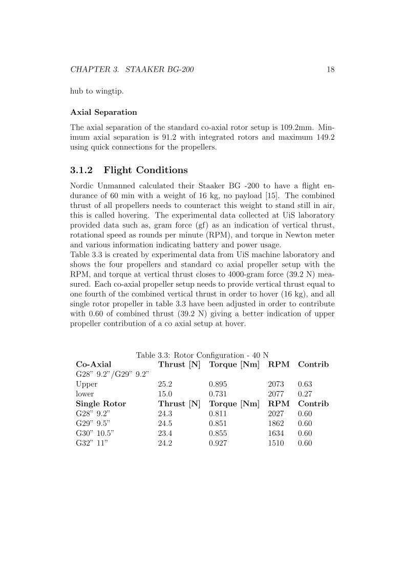
Nordic Unmanned calculated their Staaker BG -200 to have a flight en-durance of 60 min with a weight of 16 kg, no payload [15]. The combinedthrust of all propellers needs to counteract this weight to stand still in air,this is called hovering. The experimental data collected at UiS laboratoryprovided data such as, gram force (gf) as an indication of vertical thrust,rotational speed as rounds per minute (RPM), and torque in Newton meterand various information indicating battery and power usage.Table 3.3 is created by experimental data from UiS machine laboratory andshows the four propellers and standard co axial propeller setup with theRPM, and torque at vertical thrust closes to 4000-gram force (39.2 N) mea-sured. Each co-axial propeller setup needs to provide vertical thrust equal toone fourth of the combined vertical thrust in order to hover (16 kg), and allsingle rotor propeller in table 3.3 have been adjusted in order to contributewith 0.60 of combined thrust (39.2 N) giving a better indication of upperpropeller contribution of a co axial setup at hover.
Table 3.3: Rotor Configuration - 40 NCo-Axial Thrust [N] Torque [Nm] RPM ContribG28” 9.2”/G29” 9.2”Upper 25.2 0.895 2073 0.63lower 15.0 0.731 2077 0.27Single Rotor Thrust [N] Torque [Nm] RPM ContribG28” 9.2” 24.3 0.811 2027 0.60G29” 9.5” 24.5 0.851 1862 0.60G30” 10.5” 23.4 0.855 1634 0.60G32” 11” 24.2 0.927 1510 0.60

CHAPTER 3. STAAKER BG-200 19
Table 3.4: Re across propeller bladePropeller G28 9.2 2000 G29 9.5 1900 G30 10.5 1600 G32 11 1500Lb/x Re Re Re Re
0.4 141,422 148,468 131,308 139,8510.5 164,150 173,557 151,863 162,5670.6 175,767 188,318 161,758 175,2090.7 176,777 195,525 164,031 177,6570.8 173,746 189,143 154,769 175,9730.9 154,554 168,502 130,154 159,835Average 164,000 177,000 149,000 165,000
Reynolds’s Number
To determine flight condition of the octocopter, Reynolds’s Number can beused to determine the flow condition of the diverted free stream across thepropeller blade. Reynolds’s number can be calculated from surface area, den-sity, kinematic viscosity and velocity as seen in equation 2.5.Velocity can be calculated using the RPMs given in table 3.3, chord line canbe measured from the 3D models of the propellers mentioned in table 3.2.And kinematic viscosity at standard atmospheric conditions, calculated Re
values in table 3.4. The cross sections is diveded ten times from gub to wingtip, Lb/x indicates the location of the corsssection along the blade length,0 being hub and 1 being wing tip. Only values that has an airfoil shape isconsidered in table.
Table 3.4 shows Re values at lowest possible rotational velocity for eachpropeller, barely hoovering, and according to the experimental data clearlyindicates that the BG-200 operates within the low Reynolds’s number flow.
Since the propeller operate within laminar, transitional and turbulentflow, it’s needed a turbulence model to solve for the fluctuations. A 2Dvalidation case will be performed in next chapter to choose the correct tur-bulence model and grid refinement levels along the boundaries. How to finda suitable CFD system to test all different option previously mentioned inthis chapter can be a challenging task. To minimize the number of steps theNASA Langley research center has a turbulence modeling resource with theobjective to provide resource for CFD developers to obtain accurate and upto date information on RANS turbulence models and to verify that modelsare implemented correctly. This thesis will use this resource to validate thechoice of turbulence model along with a grid convergence study.
Simulation of 2D Airfoil
The purpose of this chapter is to perform a turbulence model- and gridgeneration validation for Open Foam’s implementation of the turbulencemodel Spalart Allmaras, using the NASA Turbulence Modeling Resource.The NASA turbulence modeling resource will be used to establish that themodel is implemented correctly.
4.1 Validation Case 2D
The case depicts at an airfoil operating in a velocity field of Reynolds number1.52 million with an Angle of attack of 13.87 degrees, velocity at 27.13 m/sand kinematic viscosity µ = 0.1605 cm
2
s. The airfoil chord length was 90.12
cm. Experimental data provided by the turbulence model resource is theNACA 4412 surface pressure coefficients compiled in a .dat file and will beused to compare the obtained simulations results with the experimental data[18]. The turbulence modeling recourse also provide data of expected resultsusing a range of different turbulence models. Expected results using the sameturbulence model, Spalart Allmaras is;
• CL=1.7210, CD=0.02861
• CL=1.7170, CD=0.02947
Where Cl and Cd is the coefficients of lift and drag, values are SA resultsfrom two independent CFD codes, CFL32 and FUN32 [19].The CFD simulations at the turbulence modeling resource implement thesame initial conditions, but with an increased far field outer boundary, whichis set to extend hundred times the chord line. This is far more than therelatively small wind tunnel used to obtain the experimental data.This 2D simulations will be used in order to verify the choice of turbulencemodel, but also provide a way to determine level of grid refinement needed inorder to minimize computational time whilst still providing accurate results.
20
CHAPTER 4. SIMULATION OF 2D AIRFOIL 21
4.1.1 Computational Setup
Geometry and Grid Generation
Creating a high-quality mesh is case specific. For an airfoil with adverse pres-sure gradients, a fine refinement along the airfoil is needed. This is usuallyaccomplished by surface layer with start width of cell calculated to give a y+< 1. The outer boundaries should not in any way affect the airflow aroundthe airfoil and should therefore be far away from the airfoil. The grid cre-ated and used in the turbulence modeling resource had far field boundariesexceeding 100 times chord line, but the experimental tunnel was relativelysmall.This 2D case will have a grid of 25 m in both x and y direction to minimizethe effect of the boundaries as the initial grid. The boundaries are createdand named in blockMeshDict. BlockMeshDict is needed when using snap-pyHexMesh. SnappyhexMesh is used to create the surface layers needed toobtain an y+ < 1 and all the other refinement levels. In blockMeshDict thefirst refinement level, level 0 is selected by choosing how many cells blockmeshshould create along the length of x, y and z. The lowest refinement should berelative coarse, but determines how many refinement levels are needed to geta smooth transition from the last surface layer to rest of the mesh, preferablybetween 1.2 and 2. Where 2 is the expansion ratio from a higher refinementlevel to the lower, and 1.2 is the expansion ratio used between each surfacelayer.After creating blockMeshDict, a calculation of minimum wall spacing whichcorresponds to y+ < 1, which is recommended for a incompressible- , tur-bulent flow in presence of adverse pressure gradients according to the theoryunder Surface Layer.In chapter Theory, y+ can be calculated using equations 2.22, 2.23, 2.24 and2.25. Calculating wall spacing of 1.324e-5 m to achieve a y+ < 1 and with aReynolds number at 1.6e+6 at standard atmospheric conditions.Using the know wall spacing of the first layer, and the outer boundary con-ditions, the number of refinement levels needed for a smooth transition canbe calculated knowing the decreasing grid refinement level expansion ratioat 2. All data concerning the initial grid are given in table 4.1
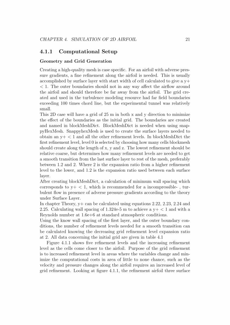
Figure 4.1.1 shows five refinement levels and the increasing refinementlevel as the cells come closer to the airfoil. Purpose of the grid refinementis to increased refinement level in areas where the variables change and min-imize the computational costs in area of little to none chance, such as thevelocity and pressure changes along the airfoil requires an increased level ofgrid refinement. Looking at figure 4.1.1, the refinement airfoil three surface
CHAPTER 4. SIMULATION OF 2D AIRFOIL 22
Table 4.1: Initial Grid CalculationsDomain Thickness 25 mRefinement level 0 thickness 0.25 my+, calculated first layer thickness 1.437 e-5 mHighest refinement level 8Highest refinement level thickness 9.766e-4 mRelative size parameter 0.7Final Layer thickness 6.835 e-4 mExpansion ratio 1.3Number of Surface Layer 16First Layer thickness 1.335 e-5 m
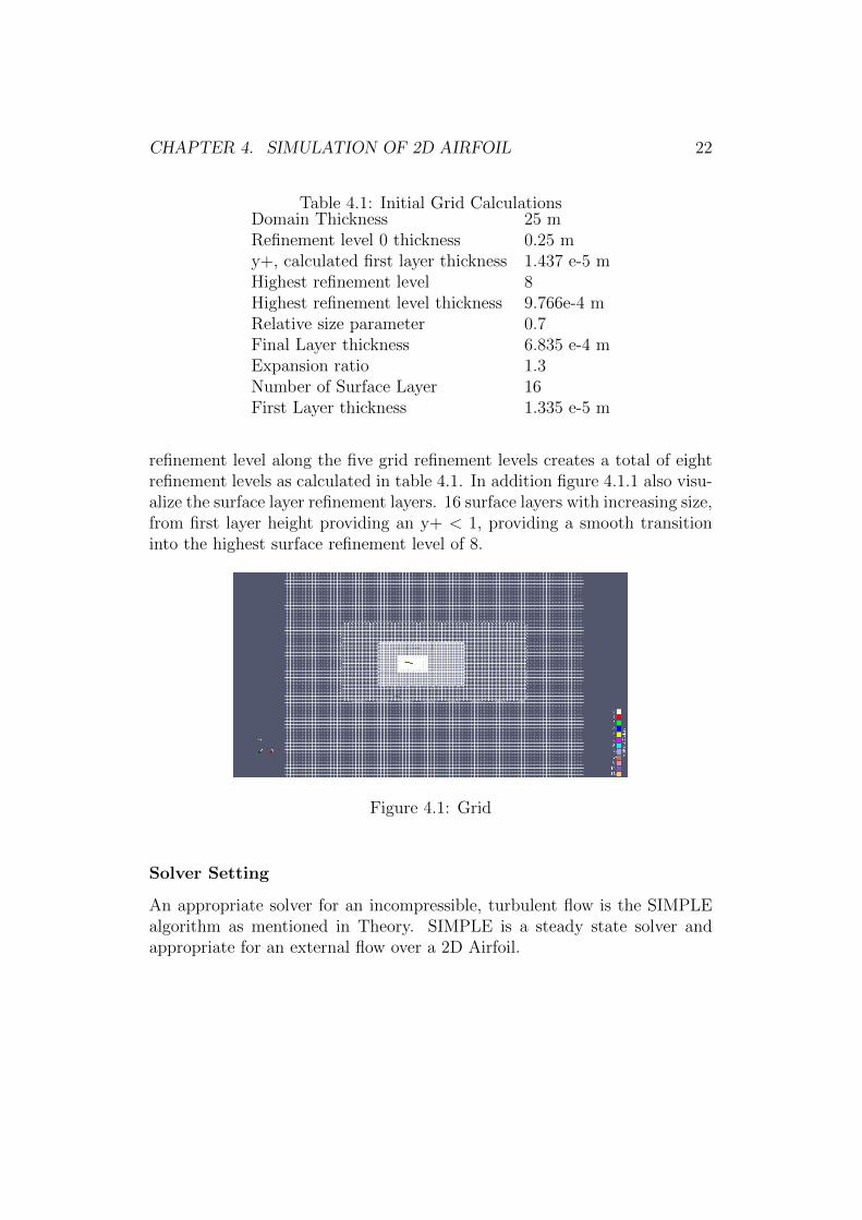
refinement level along the five grid refinement levels creates a total of eightrefinement levels as calculated in table 4.1. In addition figure 4.1.1 also visu-alize the surface layer refinement layers. 16 surface layers with increasing size,from first layer height providing an y+ < 1, providing a smooth transitioninto the highest surface refinement level of 8.
Figure 4.1: Grid
Solver Setting
An appropriate solver for an incompressible, turbulent flow is the SIMPLEalgorithm as mentioned in Theory. SIMPLE is a steady state solver andappropriate for an external flow over a 2D Airfoil.
CHAPTER 4. SIMULATION OF 2D AIRFOIL 23
Figure 4.2: Surface Layer
4.1.2 Results of the 2D airfoil simulations
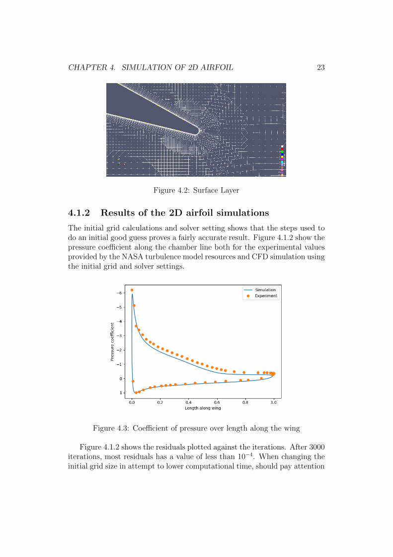
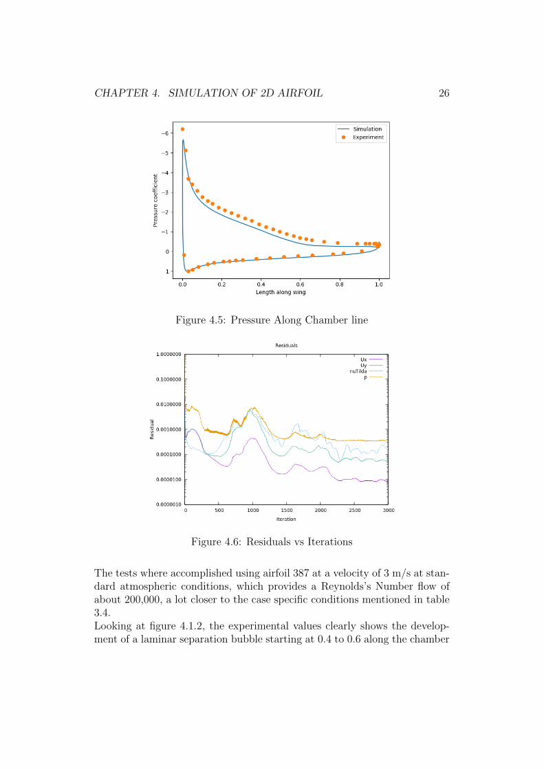
The initial grid calculations and solver setting shows that the steps used todo an initial good guess proves a fairly accurate result. Figure 4.1.2 show thepressure coefficient along the chamber line both for the experimental valuesprovided by the NASA turbulence model resources and CFD simulation usingthe initial grid and solver settings.
Figure 4.3: Coefficient of pressure over length along the wing
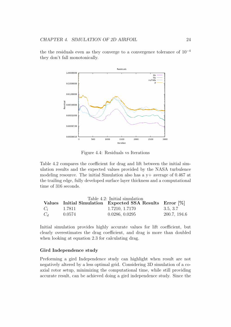
Figure 4.1.2 shows the residuals plotted against the iterations. After 3000iterations, most residuals has a value of less than 10−4. When changing theinitial grid size in attempt to lower computational time, should pay attention
CHAPTER 4. SIMULATION OF 2D AIRFOIL 24
the the residuals even as they converge to a convergence tolerance of 10−4
they don’t fall monotonically.
Figure 4.4: Residuals vs Iterations
Table 4.2 compares the coefficient for drag and lift between the initial sim-ulation results and the expected values provided by the NASA turbulencemodeling resource. The initial Simulation also has a y+ average of 0.467 atthe trailing edge, fully developed surface layer thickness and a computationaltime of 316 seconds.
Table 4.2: Initial simulationValues Initial Simulation Expected SSA Results Error [%]Cl 1.7811 1.7210, 1.7170 3.5, 3.7Cd 0.0574 0.0286, 0.0295 200.7, 194.6
Initial simulation provides highly accurate values for lift coefficient, butclearly overestimates the drag coefficient, and drag is more than doubledwhen looking at equation 2.3 for calculating drag.
Gird Independence study
Preforming a gird Independence study can highlight when result are notnegatively altered by a less optimal grid. Considering 3D simulation of a co-axial rotor setup, minimizing the computational time, while still providingaccurate result, can be achieved doing a gird independence study. Since the

CHAPTER 4. SIMULATION OF 2D AIRFOIL 25
surface layer are relative to the highest surface refinement level. All cells areaffected by changing the cell size of cells in refinement level 0. These cellsizes can be altered in blockMesh.When comparing the different simulations in this grid independence study,afully developed surface layer, and y+ < 1 is a requirement. While a minimalerror percentage at minimal computational time will be weighted against eachother. Table 4.3 shows the results from the grid Independence simulations.The simulations are named according to the number of cells of the simulationcompared to the number of cells in the initial simulation in x, or y directionin blockMesh.
Table 4.3: Grid IndependenceValues Exp. SSA 0.5 0.75 InitialS 2y+ at Wing Edge < 1 28.423 0.4931 0.4670 0.4693y+ at Wing < 1 0.4701 0.4021 0.3868 0.3857Surface Layer development 98.6 100 100 100Cl 1.7210, 1.7170 1.726 1.753 1.7811 1.776Cd 0.0286, 0.0295 0.057 0.0622 0.0574 0.0557nCells 31,172 59,221 93,338 123,338Computational Time [s] 99 196 316 442
Looking at table 4.3, all simulations provides results with very similarerror % . 0.5 simulation does not pass the preset requirements of y+ havefully developed surface layer thickness. Simulation 2 is not fully a two timesinitial simulation, but a domain size increase. This is done to verify that thefar boundaries doesn’t interfere with the simulations results. Figure 4.1.2and 4.1.2 shows the pressure coefficient along the chord line and residuals ofsimulation 0.75.
Laminar Separation Bubble
2D Validation case used in this thesis doesn’t consider low Reynolds’s num-ber flow. Knowing the turbulence model Spalart Allmaras doesn’t predictreattachment after boundary separation, the flow is considered fully turbu-lent.This leaves the validation of turbulence model; Spalart Allmaras with acrucial flaw. In an attempt to verify Spalart Allmaras as a turbulence modelvalid even for low Reynolds’s number flow. A simplified study comparingresults of Morgrado et al [11] looking into the development of Laminar Sepa-ration bubbles. Study on the E387 airfoil will be performed, testing differentAoA and their development of laminar separation bubble.
CHAPTER 4. SIMULATION OF 2D AIRFOIL 26
Figure 4.5: Pressure Along Chamber line
Figure 4.6: Residuals vs Iterations
The tests where accomplished using airfoil 387 at a velocity of 3 m/s at stan-dard atmospheric conditions, which provides a Reynolds’s Number flow ofabout 200,000, a lot closer to the case specific conditions mentioned in table3.4.Looking at figure 4.1.2, the experimental values clearly shows the develop-ment of a laminar separation bubble starting at 0.4 to 0.6 along the chamber
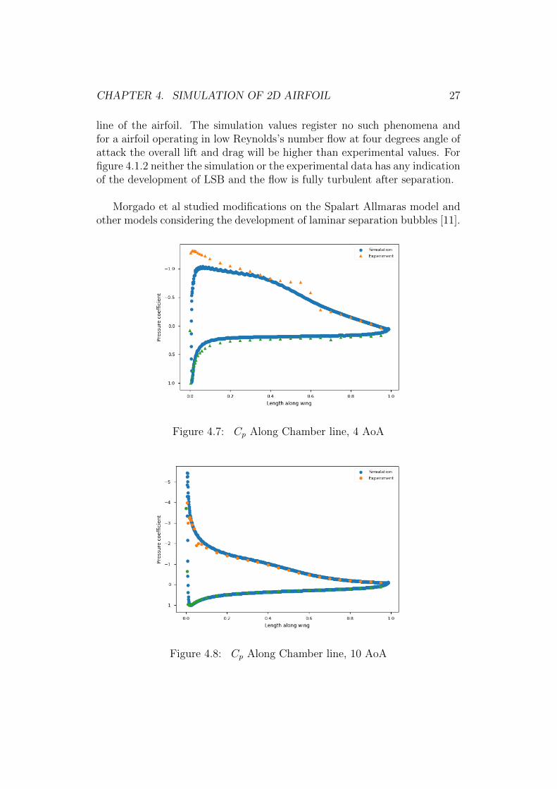
CHAPTER 4. SIMULATION OF 2D AIRFOIL 27
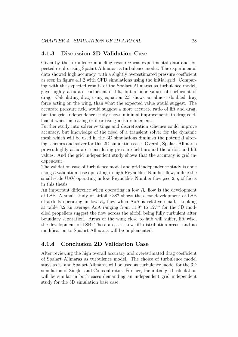
line of the airfoil. The simulation values register no such phenomena andfor a airfoil operating in low Reynolds’s number flow at four degrees angle ofattack the overall lift and drag will be higher than experimental values. Forfigure 4.1.2 neither the simulation or the experimental data has any indicationof the development of LSB and the flow is fully turbulent after separation.
Morgado et al studied modifications on the Spalart Allmaras model andother models considering the development of laminar separation bubbles [11].
Figure 4.7: Cp Along Chamber line, 4 AoA
Figure 4.8: Cp Along Chamber line, 10 AoA
CHAPTER 4. SIMULATION OF 2D AIRFOIL 28
4.1.3 Discussion 2D Validation Case
Given by the turbulence modeling resource was experimental data and ex-pected results using Spalart Allmaras as turbulence model. The experimentaldata showed high accuracy, with a slightly overestimated pressure coefficientas seen in figure 4.1.2 with CFD simulations using the initial grid. Compar-ing with the expected results of the Spalart Allmaras as turbulence model,gave highly accurate coefficient of lift, but a poor values of coefficient ofdrag. Calculating drag using equation 2.3 shows an almost doubled dragforce acting on the wing, than what the expected value would suggest. Theaccurate pressure field would suggest a more accurate ratio of lift and drag,but the grid Independence study shows minimal improvements to drag coef-ficient when increasing or decreasing mesh refinement.Further study into solver settings and discretisation schemes could improveaccuracy, but knowledge of the need of a transient solver for the dynamicmesh which will be used in the 3D simulations diminish the potential alter-ing schemes and solver for this 2D simulation case. Overall, Spalart Allmarasproves highly accurate, considering pressure field around the airfoil and liftvalues. And the grid independent study shows that the accuracy is grid in-dependent.The validation case of turbulence model and grid independence study is doneusing a validation case operating in high Reynolds’s Number flow, unlike thesmall scale UAV operating in low Reynolds’s Number flow ,see 2.5, of focusin this thesis.An important difference when operating in low Re flow is the developmentof LSB. A small study of airfoil E387 shows the clear development of LSBof airfoils operating in low Re flow when AoA is relative small. Lookingat table 3.2 an average AoA ranging from 11.9 to 12.7 for the 3D mod-elled propellers suggest the flow across the airfoil being fully turbulent afterboundary separation. Areas of the wing close to hub will suffer, lift wise,the development of LSB. These areas is Low lift distribution areas, and nomodification to Spalart Allmaras will be implemented.
4.1.4 Conclusion 2D Validation Case
After reviewing the high overall accuracy and overestimated drag coefficientof Spalart Allmaras as turbulence model. The choice of turbulence modelstays as is, and Spalart Allmaras will be used as turbulence model for the 3Dsimulation of Single- and Co-axial rotor. Further, the initial grid calculationwill be similar in both cases demanding an independent grid independentstudy for the 3D simulation base case.
CHAPTER 4. SIMULATION OF 2D AIRFOIL 29
There will be no modifications done to the Spalart Allmaras turbulence modelconsidering the development of laminar separation bubbles.
Simulation of 3D single- and co-axial rotor
This chapter is the is going to explain choices made when simulating thesingle- and co- axial rotor configuration. Turbulence model validated in 2Dsimulation of a airfoil is going to be used without modifications. While thegrid generation part of the 3D simulations will undergo the same process ofdetermining grid as the 2D simulations.To verify the result of the 3D simulation, the experimental values from UiSlaboratory will be used for comparison. The experimental values are gatheredusing a test rig of a coaxial rotor thrust stand controlled by RCBenchmark.RCBenchmark lets the operator control the change in % of throttle input,and provides information of torque, thrust, voltage, ampere, motor opticalspeed and a mechanical power usage. The experimental results have beenvalidated using the engine providers test report with same propeller andvoltage. Since the experimental data includes a wide range of RPM (motoroptical speed) values, a specific RPM values is easily compared. The RPMvalue used in calculations for Reynolds number and propeller velocities intable 3.4 is going to be used in the 3D simulations.
5.1 3D - Single Rotor simulations
The initial grid and solver setting will be as similar to the 2D validation caseas possible. Although a similar, but transient solver is required for a dynamicmesh. Pimple instead of SIMPLE will be used in 3D simulations.The rotational velocity as initial velocity will be similar to the rotationalspeed of the standard rotor setup which Nordic Unmanned is using today athoover, see table 3.4. Using 2000 RPM as initial velocity requires and AMImoving the propeller with a rotational speed of 210 rad/s. AMI stands for
30
CHAPTER 5. SIMULATION OF 3D SINGLE- AND CO-AXIAL ROTOR31
Table 5.1: Initial GridDomain thickness 8 mRefinement level 0 thickness 0.05 my+, calculated first layer thickness 6.211 e-6 mHighest refinement level 7Highest refinement level thickness 3.905 e-4 mRelative size parameter 0.5Final layer thickness 1.953 e-4 mExpansion ratio 1.3Number of Surface Layer 15Final layer thickness 4.960 e-6 m
Arbitrary Mesh Interface, and is used when simulating rotating geometries,where there is a moving- and a stationary part. The AMI should be placedaround the propeller, small enough to not interfere with the AMI placedaround the lower propeller in a coaxial setup.In order to increase flight endurance, a co axial propeller configuration op-timized for operating in the International Standard Metric Conditions withrelations to pressure and temperature.The initial axial separation will be standard distance between mounted pro-peller of 109.2 mm with a small adjustment for propeller width leaving theinitial axial separation at z0 = 115 mm.
5.1.1 Computational Setup
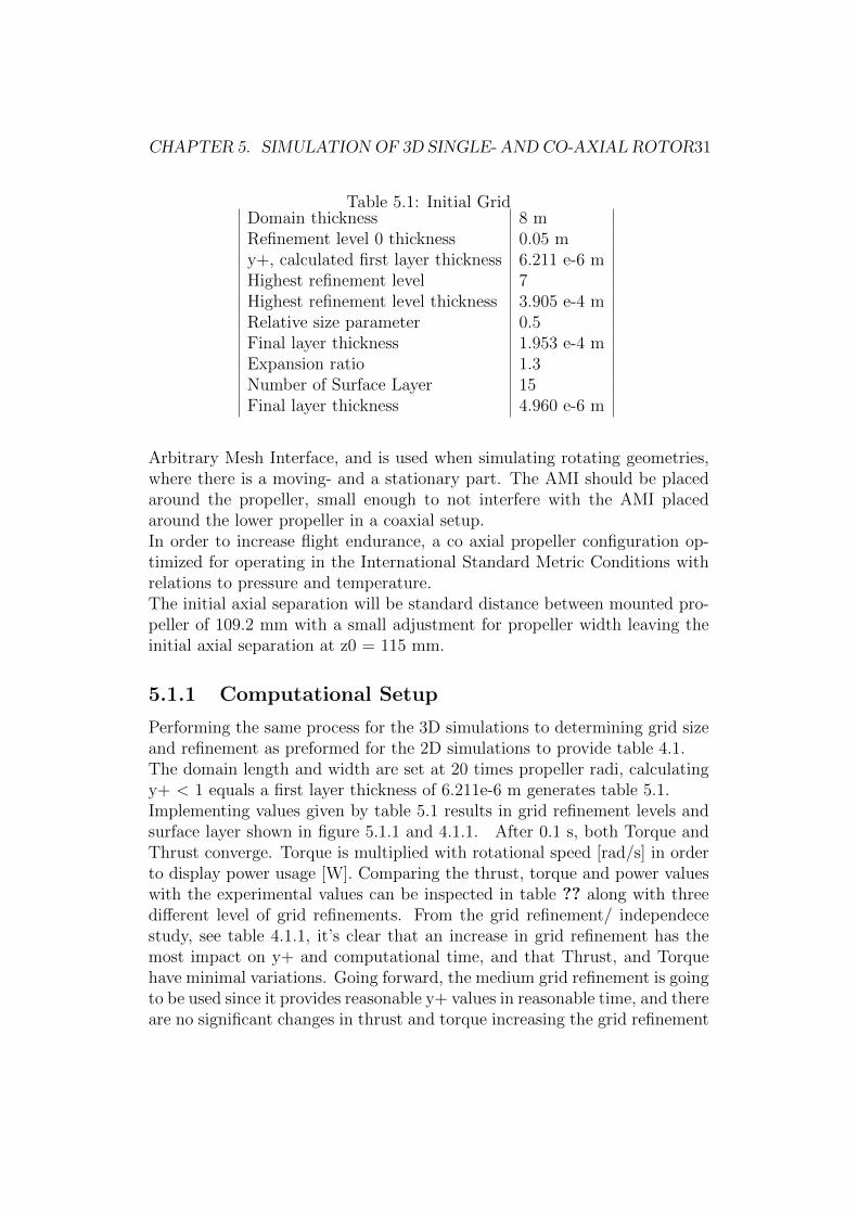
Performing the same process for the 3D simulations to determining grid sizeand refinement as preformed for the 2D simulations to provide table 4.1.The domain length and width are set at 20 times propeller radi, calculatingy+ < 1 equals a first layer thickness of 6.211e-6 m generates table 5.1.Implementing values given by table 5.1 results in grid refinement levels andsurface layer shown in figure 5.1.1 and 4.1.1. After 0.1 s, both Torque andThrust converge. Torque is multiplied with rotational speed [rad/s] in orderto display power usage [W]. Comparing the thrust, torque and power valueswith the experimental values can be inspected in table ?? along with threedifferent level of grid refinements. From the grid refinement/ independecestudy, see table 4.1.1, it’s clear that an increase in grid refinement has themost impact on y+ and computational time, and that Thrust, and Torquehave minimal variations. Going forward, the medium grid refinement is goingto be used since it provides reasonable y+ values in reasonable time, and thereare no significant changes in thrust and torque increasing the grid refinement
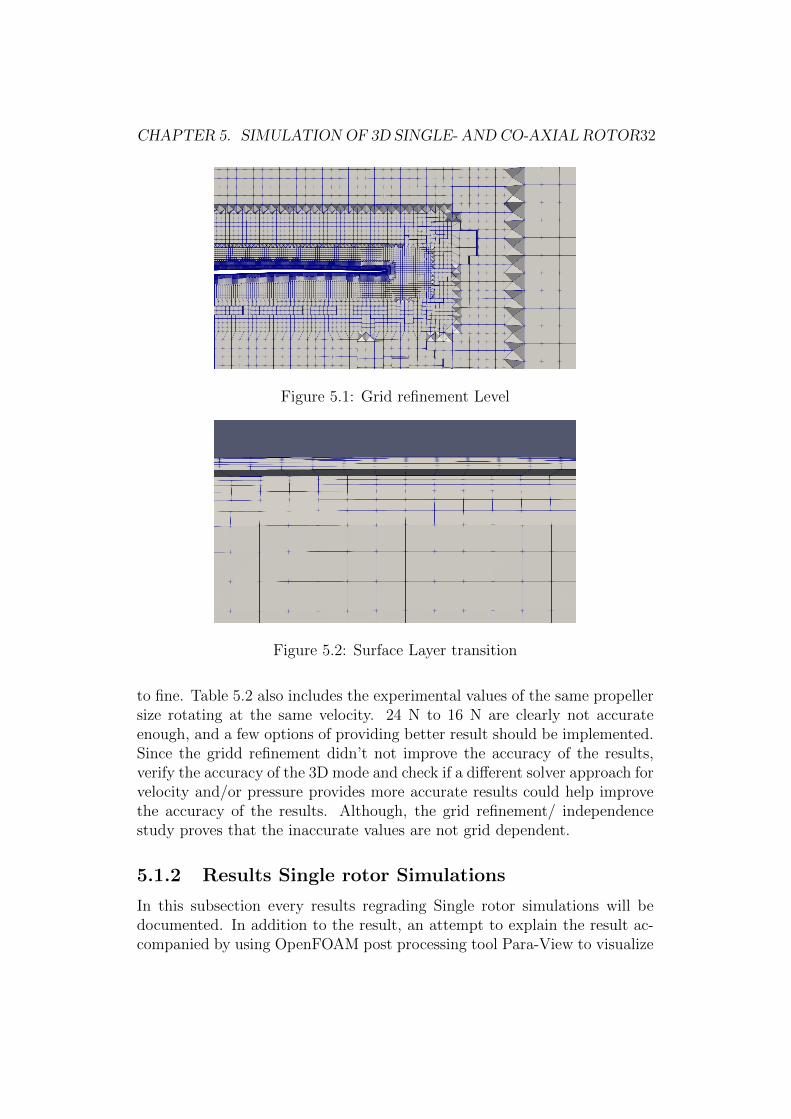
CHAPTER 5. SIMULATION OF 3D SINGLE- AND CO-AXIAL ROTOR32
Figure 5.1: Grid refinement Level
Figure 5.2: Surface Layer transition
to fine. Table 5.2 also includes the experimental values of the same propellersize rotating at the same velocity. 24 N to 16 N are clearly not accurateenough, and a few options of providing better result should be implemented.Since the gridd refinement didn’t not improve the accuracy of the results,verify the accuracy of the 3D mode and check if a different solver approach forvelocity and/or pressure provides more accurate results could help improvethe accuracy of the results. Although, the grid refinement/ independencestudy proves that the inaccurate values are not grid dependent.
5.1.2 Results Single rotor Simulations
In this subsection every results regrading Single rotor simulations will bedocumented. In addition to the result, an attempt to explain the result ac-companied by using OpenFOAM post processing tool Para-View to visualize
CHAPTER 5. SIMULATION OF 3D SINGLE- AND CO-AXIAL ROTOR33
Table 5.2: Grid Refinement for Single 28” Propeller28S Coarse 28S Medium 28S Fine Exp. Values
y+ Propeller 2.392 1.877 1.317nCells 4,247,427 6,123,401 8,730,655cTime [s] 60,748 127,786 175,277Thrust [N] 15.902 16.181 16.338 24.358Torque [Nm] 0.544 0.544 0.544 0.808Power [W] 113.867 113.960 113.894 171.059
the explanation. All figures are either created using plots from simulationdata or graphical representations using Para-view.
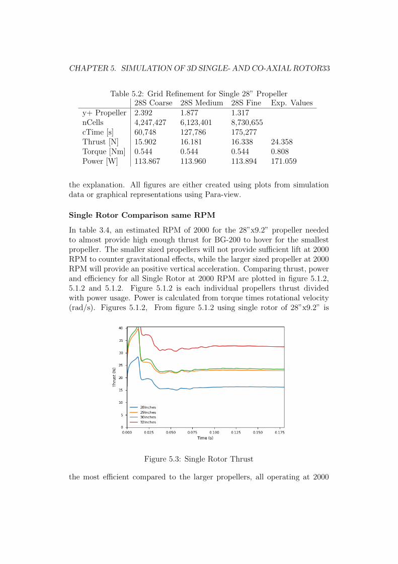
Single Rotor Comparison same RPM
In table 3.4, an estimated RPM of 2000 for the 28”x9.2” propeller neededto almost provide high enough thrust for BG-200 to hover for the smallestpropeller. The smaller sized propellers will not provide sufficient lift at 2000RPM to counter gravitational effects, while the larger sized propeller at 2000RPM will provide an positive vertical acceleration. Comparing thrust, powerand efficiency for all Single Rotor at 2000 RPM are plotted in figure 5.1.2,5.1.2 and 5.1.2. Figure 5.1.2 is each individual propellers thrust dividedwith power usage. Power is calculated from torque times rotational velocity(rad/s). Figures 5.1.2, From figure 5.1.2 using single rotor of 28”x9.2” is
Figure 5.3: Single Rotor Thrust
the most efficient compared to the larger propellers, all operating at 2000
CHAPTER 5. SIMULATION OF 3D SINGLE- AND CO-AXIAL ROTOR34
Figure 5.4: Single Rotor Power
Figure 5.5: Efficiency Single Rotor
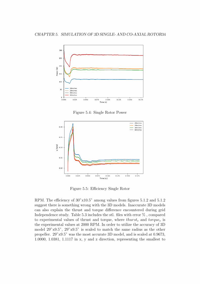
RPM. The efficiency of 30”x10.5” among values from figures 5.1.2 and 5.1.2suggest there is something wrong with the 3D models. Inaccurate 3D modelscan also explain the thrust and torque difference encountered during gridIndependence study. Table 5.3 includes the stl. files with error % , comparedto experimental values of thrust and torque, where thurste and torquee isthe experimental values at 2000 RPM. In order to utilize the accuracy of 3Dmodel 29”x9.5”, 29”x9.5” is scaled to match the same radius as the otherpropeller. 29”x9.5” was the most accurate 3D model, and is scaled at 0.9673,1.0000, 1.0381, 1.1117 in x, y and z direction, representing the smallest to
CHAPTER 5. SIMULATION OF 3D SINGLE- AND CO-AXIAL ROTOR35
largest propeller.Looking at the increased accuracy of the scaled propeller compared to
Table 5.3: 3D model accuracy at 2000 RPMPropeller Thrust [N] Thruste [N] [%] Torque [Nm] Torquee [Nm] [%]28” 9.2” 16.18 24.36 0.66 0.544 0.808 0.6729” 9.5” 22.8 26.9 0.85 0.87 0.94 0.9330” 10.5” 23.4 34.6 0.68 0.86 1.26 0.6832” 11” 32.5 41.1 0.79 1.28 1.57 0.82
the experimental result, the scaled propeller will be used when comparingdifferent sized propeller when it seems more likely to provide a more realisticresult. All simulations will not be rerun using scaled propellers, but onlyhighlighted when scaled propellers are used.
RPM range
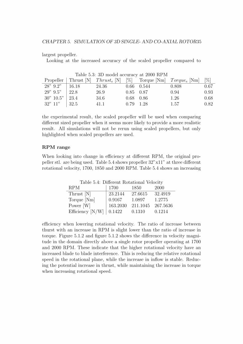
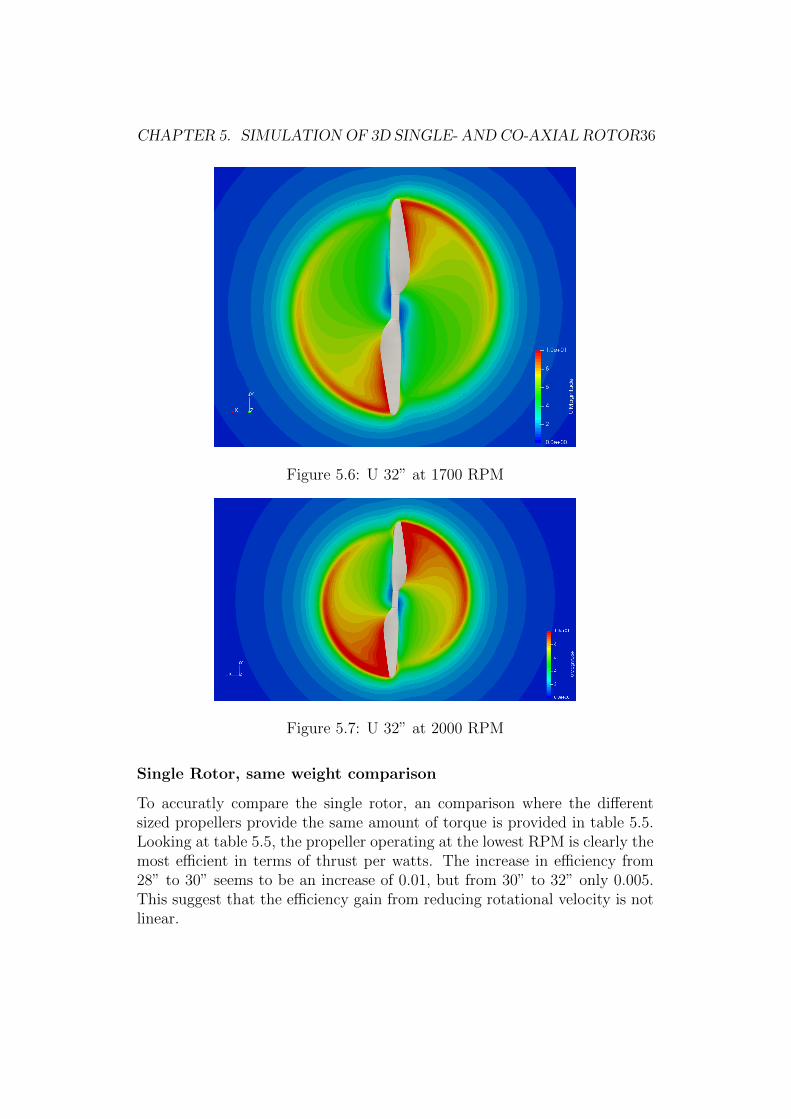
When looking into change in efficiency at different RPM, the original pro-peller stl. are being used. Table 5.4 shows propeller 32”x11” at three differentrotational velocity, 1700, 1850 and 2000 RPM. Table 5.4 shows an increasing
Table 5.4: Different Rotational VelocityRPM 1700 1850 2000Thrust [N] 23.2144 27.6615 32.4919Torque [Nm] 0.9167 1.0897 1.2775Power [W] 163.2030 211.1045 267.5636Efficiency [N/W] 0.1422 0.1310 0.1214
efficiency when lowering rotational velocity. The ratio of increase betweenthurst with an increase in RPM is slight lower than the ratio of increase intorque. Figure 5.1.2 and figure 5.1.2 shows the difference in velocity magni-tude in the domain directly above a single rotor propeller operating at 1700and 2000 RPM. These indicate that the higher rotational velocity have anincreased blade to blade interference. This is reducing the relative rotationalspeed in the rotational plane, while the increase in inflow is stable. Reduc-ing the potential increase in thrust, while maintaining the increase in torquewhen increasing rotational speed.
CHAPTER 5. SIMULATION OF 3D SINGLE- AND CO-AXIAL ROTOR36
Figure 5.6: U 32” at 1700 RPM
Figure 5.7: U 32” at 2000 RPM
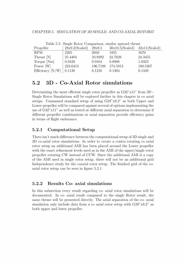
Single Rotor, same weight comparison
To accuratly compare the single rotor, an comparison where the differentsized propellers provide the same amount of torque is provided in table 5.5.Looking at table 5.5, the propeller operating at the lowest RPM is clearly themost efficient in terms of thrust per watts. The increase in efficiency from28” to 30” seems to be an increase of 0.01, but from 30” to 32” only 0.005.This suggest that the efficiency gain from reducing rotational velocity is notlinear.
CHAPTER 5. SIMULATION OF 3D SINGLE- AND CO-AXIAL ROTOR37
Table 5.5: Single Rotor Comparison, similar upward thrustPropeller 28x9.2(Scaled) 29x9.5 30x10.5(Scaled) 32x11(Scaled)RPM 2265 2050 1855 1670Thrust [N] 25.4404 23.9292 22.7628 24.3455Torque [Nm] 0.9429 0.9164 0.8988 1.0323Power [W] 223.6413 196.7198 174.5913 180.5307Efficiency [N/W] 0.1138 0.1216 0.1304 0.1349
5.2 3D - Co-Axial Rotor simulations
Determining the most efficient single rotor propeller as G32”x11” from 3D -Single Rotor Simulations will be explored further in this chapter in co axialsetups. Unmanned standard setup of using G28”x9.2” as both Upper andLower propeller will be compared against several of options implementing theuse of G32”x11” as well as tested at different axial separation to determine ifdifferent propeller combinations or axial separation provide efficiency gainsin terms of flight endurance.
5.2.1 Computational Setup
There isn’t much difference between the computational setup of 3D single and3D co-axial rotor simulations. In order to create a contra rotating co axialrotor setup an additional AMI has been placed around the Lower propellerwith the exact refinement levels used as in the AMI of the upper/single rotorpropeller rotating CW instead of CCW. Since the additional AMI is a copyof the AMI used in single rotor setup, there will not be an additional gridIndependence study for the coaxial rotor setup. The finished grid of the co-axial rotor setup can be seen in figure 5.2.1.
5.2.2 Results Co- axial simulations
In this subsection every result regarding co- axial rotor simulations will bedocumented. In co- axial result compared to the single Rotor result, thesame thrust will be presented directly. The axial separation of the co- axialsimulation only include data from a co axial rotor setup with G28”x9.2” asboth upper and lower propeller.
CHAPTER 5. SIMULATION OF 3D SINGLE- AND CO-AXIAL ROTOR38
Figure 5.8: Finished Grid Co Axial
Co-axial rotor comparison same weight
Experimental data from UiS labratory is available for standard co axial rotorsetup and given in table 3.3. This data provides combined 40.2 N. All coaxial simulations in table 5.6 have been a adjusted with 200 RPM in orderto provide about the same upward thrust as the experimental values. The
Table 5.6: Co-Axial rotor Comparison, same upward thrustThrust [N] Upper Lower CombinedU28 L28 24.3974 16.5092 40.9066U28 L32 18.4611 24.5950 43.0561U32 L32 23.8808 16.3850 40.2658Torque [Nm]U28 L28 0.9835 0.8507 1.8342U28 L32 0.7376 1.2206 1.9582U32 L32 1.0828 0.9585 2.0413Efficiency [N/W]U28 L28 0.1150 0.0900 0.1034U28 L32 0.1343 0.1159 0.1231U32 L32 0.1404 0.1088 0.1256
upper propeller in these rotor setups are all acting as an isolated Single rotor,see table 5.6, the difference of U28 L32 and U28 L28 for the upper propelleris because of reduction in rotational velocity by the increased contribution ofthe lower 32” propeller. And as witnessed in Single Rotor same thrust sub-section, the most efficient upper propeller is the largest propeller operatingwith the lowest rotational speed.
CHAPTER 5. SIMULATION OF 3D SINGLE- AND CO-AXIAL ROTOR39
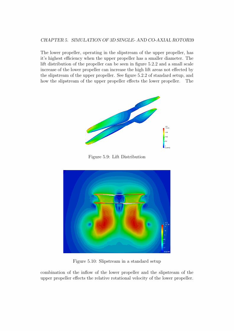
The lower propeller, operating in the slipstream of the upper propeller, hasit’s highest efficiency when the upper propeller has a smaller diameter. Thelift distribution of the propeller can be seen in figure 5.2.2 and a small scaleincrease of the lower propeller can increase the high lift areas not effected bythe slipstream of the upper propeller. See figure 5.2.2 of standard setup, andhow the slipstream of the upper propeller effects the lower propeller. The
Figure 5.9: Lift Distribution
Figure 5.10: Slipstream in a standard setup
combination of the inflow of the lower propeller and the slipstream of theupper propeller effects the relative rotational velocity of the lower propeller.
CHAPTER 5. SIMULATION OF 3D SINGLE- AND CO-AXIAL ROTOR40
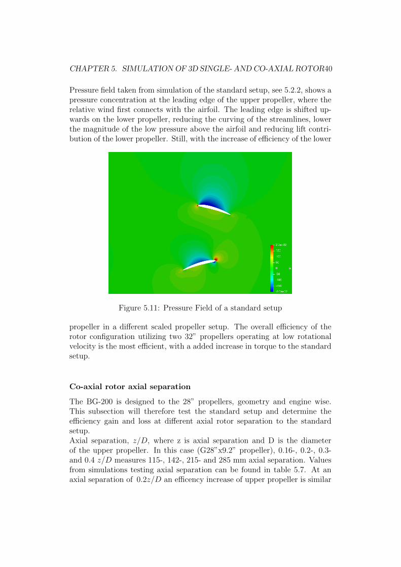
Pressure field taken from simulation of the standard setup, see 5.2.2, shows apressure concentration at the leading edge of the upper propeller, where therelative wind first connects with the airfoil. The leading edge is shifted up-wards on the lower propeller, reducing the curving of the streamlines, lowerthe magnitude of the low pressure above the airfoil and reducing lift contri-bution of the lower propeller. Still, with the increase of efficiency of the lower
Figure 5.11: Pressure Field of a standard setup
propeller in a different scaled propeller setup. The overall efficiency of therotor configuration utilizing two 32” propellers operating at low rotationalvelocity is the most efficient, with a added increase in torque to the standardsetup.
Co-axial rotor axial separation
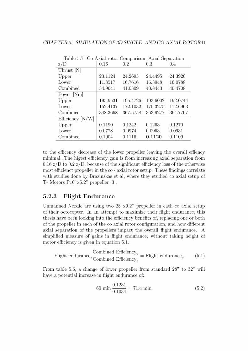
The BG-200 is designed to the 28” propellers, geometry and engine wise.This subsection will therefore test the standard setup and determine theefficiency gain and loss at different axial rotor separation to the standardsetup.Axial separation, z/D, where z is axial separation and D is the diameterof the upper propeller. In this case (G28”x9.2” propeller), 0.16-, 0.2-, 0.3-and 0.4 z/D measures 115-, 142-, 215- and 285 mm axial separation. Valuesfrom simulations testing axial separation can be found in table 5.7. At anaxial separation of 0.2z/D an efficency increase of upper propeller is similar
CHAPTER 5. SIMULATION OF 3D SINGLE- AND CO-AXIAL ROTOR41
Table 5.7: Co-Axial rotor Comparison, Axial Separationz/D 0.16 0.2 0.3 0.4Thrust [N]Upper 23.1124 24.2693 24.4495 24.3920Lower 11.8517 16.7616 16.3948 16.0788Combined 34.9641 41.0309 40.8443 40.4708Power [Nm]Upper 195.9531 195.4726 193.6002 192.0744Lower 152.4137 172.1032 170.3275 172.6963Combined 348.3668 367.5758 363.9277 364.7707Efficiency [N/W]Upper 0.1190 0.1242 0.1263 0.1270Lower 0.0778 0.0974 0.0963 0.0931Combined 0.1004 0.1116 0.1120 0.1109
to the efficency decrease of the lower propeller leaving the overall effiencyminimal. The higest efficiency gain is from increasing axial separation from0.16 z/D to 0.2 z/D, because of the significant efficiency loss of the otherwisemost efficienct propeller in the co - axial rotor setup. These findings correlatewith studies done by Brazinskas et al, where they studied co axial setup ofT- Motors P16”x5.2” propeller [3].
5.2.3 Flight Endurance
Unmanned Nordic are using two 28”x9.2” propeller in each co axial setupof their octocopter. In an attempt to maximize their flight endurance, thisthesis have been looking into the efficiency benefits of, replacing one or bothof the propeller in each of the co axial rotor configuration, and how differentaxial separation of the propellers impact the overall flight endurance. Asimplified measure of gains in flight endurance, without taking height ofmotor efficiency is given in equation 5.1.
Flight endurancesCombined EfficiencypCombined Efficiencys
= Flight endurancep (5.1)
From table 5.6, a change of lower propeller from standard 28” to 32” willhave a potential increase in flight endurance of:
60 min0.1231
0.1034= 71.4 min (5.2)
CHAPTER 5. SIMULATION OF 3D SINGLE- AND CO-AXIAL ROTOR42
Chaning both propellers to 32” and utilizing the most efficienct co - axialsetup studied in this thesis have a potential increase in flight endurance of:
60 min0.1256
0.1034= 72.9 min (5.3)
From table 5.7, the combined efficiency of axial separation of 0.3 z/D is0.1120 N/W which is an increase of 0.116 from standard setup considering40 N, will give a potential increase in flight endurance of:
60 min0.1120
0.1004= 66.9 min (5.4)

Conclusion
In this thesis, a co axial propeller configuration optimization study has beenmade of four different propellers at four different axial separation distances.Computational Fluid Dynamics simulations of 3D co-axial rotor simulation,3D single rotor simulation and 2D airfoil simulation was completed usingOpenFOAM. The 2D airfoil simulation was used to validate the turbulencemodel and grid Independence study used in both 3D simulations.3D simulation of the single rotor cases was completed in order to determinethe efficiency of each propeller individually. Only the most efficient propellerwas compared to the standard setup, to verify the propeller combination effi-ciency. Every propeller combination was tested to determine which co- axialrotor configuration provided the highest possible flight endurance.Results revealed that the co axial propeller setup which provided thrust equalto the one forth of the total weight demand, was the propeller operating atthe lowest rotational velocity. The importance of controlling rotational veloc-ity because of blade to blade interference is crucial when optimizing co-axialpropeller configuration for flight endurance.Changing the standard setup of two 28”x9.2” propeller with two 32”x11”propeller increased to theoretical flight endurance at zero payload from 60min to 72.9 min, while only chancing the lower propeller with a 32”x11”propeller still provided 11.4 min.The highest efficiency gain on the lower propeller was found when using asmall upper, and larger lower propeller, because of minimizing the effect ofthe slipstream of the upper propeller.Different axial separation simulations showed that an increase of axial sepa-ration from 0.16 z/D to 0.2 z/D had a positive effect on efficiency. Furtherincreasing the axial separation showed minimal gains in terms of efficiency,but the entire range from 0.2 to 0.4 seemed fairly stable. A standard setupwith increased axial separation to 0.3 z/D will provide an efficiency gain tothe standard 0.16 z/D which account for fluctuations in rotational veloc-ity. The potential increase in flight endurance at zero payload with axial
43
CHAPTER 6. CONCLUSION 44
separation of 0.3 z/D is about 67 min.
6.1 Computational Fluid Dynamics
CFD analysis of fluid problems is numerical approximation of the actual fluidproblems. Increasing the accuracy of a CFD simulation can be achieved byincreasing grid refinement, fully develop surface layer and select higher orderand more accurate discretisation schemes. Every improvement comes witha increased computational costs, and a selection between available time andcomputational power against simulation accuracy must be made.CFD simulations in this thesis have good agreement with the experimentalresults from UiS machine laboratory, but with low accuracy. This providesan opportunity to run more experiments at a lower accuracy, while still ob-taining simulations with good agreement.With the development of computer- hardware and software, and the contin-ues increase in computational power, some of the present options made toreduce computational time will be neglected. This will potentially lower therequirements to the CFD designer and increase the overall accuracy of CFDsimulations. Making the performance of this thesis a wonderful step into theworld of CFD.
6.2 Further Work
This section is a quick run through of potential areas of study or improve-ments that have been encountered throughout this thesis.
Increased accuracy of simulations
All 3D models accuracy should be tested using CMM, to verify and improvethe inaccuracy of the simulations. All 3D models is also infinitely stiff, andmight provide more realistic results being elastic. Secondly, recreating thesimulation files and choose more accurate discreatisation schemes, while stillbeing stable and a fully developed surface layer around the wing tips.
More simulations
A wider range of simulations in the axial separation study an additional sim-ulations testing different propeller combinations. Testing different propellercombinations should also be included in the co - axial rotor comparison study,

CHAPTER 6. CONCLUSION 45
especially 29”, which Nordic Unmanned already cleared for use at lower ro-tational velocities. Modifications done to the geometry and inlet conditioncan easily be tested using small adjustments to the present simulations files.Modifications such as, inlet velocity, co rotating propeller study, increasednumber of blades, and optimize the design of the lower propeller would beinteresting to simulate when looking at the potential in increased flight en-durance.
References
[1] Taking flight, Library Catalog: www.economist.com. [Online]. Avail-able: http://www.economist.com/technology-quarterly/2017-06-08/civilian-drones (visited on 05/06/2020).
[2] Nordic Unmanned - One of the leading drone service provider in Eu-rope, en-US, Library Catalog: nordicunmanned.com. [Online]. Avail-able: https://nordicunmanned.com/about/ (visited on 05/05/2020).
[3] M. Brazinskas, S. Prior, and J. Scanlan, “An Empirical Study of Over-lapping Rotor Interference for a Small Unmanned Aircraft PropulsionSystem”, en, Aerospace, vol. 3, no. 4, p. 32, Oct. 2016, issn: 2226-4310. doi: 10.3390/aerospace3040032. [Online]. Available: http:
//www.mdpi.com/2226-4310/3/4/32 (visited on 05/05/2020).
[4] S. D. Prior, “Reviewing and Investigating the Use of Co-Axial Ro-tor Systems in Small UAVs”, en, International Journal of Micro AirVehicles, vol. 2, no. 1, pp. 1–16, Mar. 2010, issn: 1756-8293, 1756-8307. doi: 10.1260/1756-8293.2.1.1. [Online]. Available: http://journals.sagepub.com/doi/10.1260/1756-8293.2.1.1 (visitedon 05/05/2020).
[5] S. Walker, “Langley Research Center Hampton, Virginia”, en, p. 234,
[6] P. R. Spalart and C. L. Rumsey, “Turbulence Model Behavior in LowReynolds Number Regions of Aerodynamic Flowfields”, eng, 2008. [On-line]. Available: http://ntrs.nasa.gov/search.jsp?R=20090017753(visited on 06/23/2020).
[7] J. G. Leishman and S. Ananthan, “AERODYNAMIC OPTIMIZA-TION OF A COAXIAL PROPROTOR”, en, p. 23,
[8] Yunus A. Cengel, Fluid mechanics: fundamentals and applications, eng,3rd ed. in SI units. Boston: McGraw-Hill, 2014, Pages: XXIV, 986, isbn:978-1-259-01122-1.
46
REFERENCES 47
[9] H. K. Versteeg, An introduction to computational fluid dynamics: the fi-nite volume method, eng, 2nd ed. Harlow: Pearson/Prentice Hall, 2007,Pages: XII, 503, isbn: 978-0-13-127498-3.
[10] P. Spalart and S. Allmaras, “A One-Equation Turbulence Model forAerodynamic Flows”, AIAA, vol. 439, Jan. 1992. doi: 10.2514/6.1992-439.
[11] J. Morgado, R. Vizinho, M. Silvestre, and J. Pascoa, “XFOIL vs CFDperformance predictions for high lift low Reynolds number airfoils”,en, Aerospace Science and Technology, vol. 52, pp. 207–214, May 2016,issn: 12709638. doi: 10.1016/j.ast.2016.02.031. [Online]. Avail-able: https://linkinghub.elsevier.com/retrieve/pii/S1270963816300839(visited on 05/05/2020).
[12] OpenCFD, Numerical schemes, en, Library Catalog: www.openfoam.com.[Online]. Available: http://www.openfoam.com (visited on 06/24/2020).
[13] J. Nobrega and H. Jasak, Eds., OpenFOAM R© : Selected Papers ofthe 11th Workshop, en. Springer International Publishing, 2019, isbn:978-3-319-60845-7. doi: 10.1007/978- 3- 319- 60846- 4. [Online].Available: https://www.springer.com/gp/book/9783319608457
(visited on 06/14/2020).
[14] M. Tomislav, The OpenFOAM Technology Primer. Sourceflux, 2014,isbn: 978-3-00-046757-8.
[15] STAAKER BG200 - Nordicunmanned - Leading European Provider,en-US, Library Catalog: nordicunmanned.com, Dec. 2019. [Online].Available: https : / / nordicunmanned . com / products / unmanned -
systems-drones/staaker-bg200/ (visited on 05/19/2020).
[16] Mikell P. Groover, Automation, production systems, and computer-integrated manufacturing, eng, 3rd ed. Upper Saddle River, N.J: Pear-son Prentice-Hall, 2008, Pages: XVI, 815, isbn: 978-0-13-239321-8.
[17] Creaform, HandySCAN 3D Scanner for 3D Metrology, en, Library Cat-alog: www.creaform3d.com. [Online]. Available: https://www.creaform3d.com/en/portable-3d-scanner-handyscan-3d/technical-specifications
(visited on 06/14/2020).
[18] 2D NACA 4412 Airfoil Trailing Edge Separation. [Online]. Available:https://turbmodels.larc.nasa.gov/naca4412sep_val.html (vis-ited on 06/14/2020).
[19] D. C. Jespersen, T. H. Pulliam, and M. L. Childs, “OVERFLOW Tur-bulence Modeling Resource Validation Results”, en, p. 176,