Embed Size (px)
Citation preview
Guidelines for Satellite Tracking 1
X
Guidelines for Satellite Tracking
DusanVuckovic, PetarRajkovic, DraganJankovic and Olivera Pavic Faculty of Electronic Engineering, University of Nis
Serbia
1. Looking at the sky
Whether you are willing to confess or not, the most useful instrument for observing the sky, by day or by night, is the naked eye. For the ones with less experience, it is important to become familiar with the general aspects of the sky. Wide field of view that human eye is naturally equipped with is ideal for this purpose. Binoculars and telescope are also indispensable tools, but they may be introduced, once the familiarity with the sky is established. Since celestial bodies have a tendency of moving, it is very hard to predict their future position. It is the big mathematical engine that will help us pinpoint the object in the sky, so we would be able to look there, or point our telescope. Many objects in the sky look very similar. In NASA’s1 1997 report it’s being said that there are 25,000 man-made objects in space. 8681 are currently orbiting Earth, and 16,000 objects are in a state of decay. Course, situation is quite different today, considering that’s been 13 years since that report was published. Large portion of 16,000 objects are orbital debris: parts, such as nosecone shrouds, lens, hatch covers, rocket bodies, payloads that have disintegrated or exploded, and even objects that “escape” from manned spacecraft during operations. Most of these objects are small, but quite a few are large enough to be seen with unaided eye. Additional difficulties come with the fact that many military or government satellites are painted in black, thus very hard to spot even with very sophisticated optical instruments. Three things become immediately obvious when you take a look at the night sky. Not all the stars look the same, also stars twinkle, and finally, it’s easy to arrange stars into recognizable patterns. Some stars are bright, some are less bright and some almost too dim to see with naked eye. Astronomers have had to devise some means of expression the variation precisely. Ancient Greek astronomer Hipparchos was the first to produce the star catalogue, introducing the new value of importance, or magnitude, the star had. He thought that important stars should be of higher importance and termed them magnitude 1. Those somewhat dimmer he considered of second importance (magnitude 2), and so on. Altogether, he created six classes of star’s magnitudes. At that time, he was not aware of the fact that his six divisions were based on the way the human eye recognizes a brightness
1NASA – US National Aeronautics and Space Administration
1
www.intechopen.com

difference, where one object seems half as bright as another does. It was later discovered that Hipparchos’ six magnitudes give a difference between magnitude 1 and 6 of 100 times. Although this system has been refined, most scientists use six degrees magnitude system to explain the stars, or other celestial body’s brightness in the sky. Predictions are necessary if you want to observe satellites or other objects in the sky. You have to know where to look and when to look. Time is very important, so a stopwatch with an accuracy of at least 0.5 seconds is essential. Set the watch by radio time signals, or by telephone system’s speaking clock. More innovative method would include mobile phone with stopwatch that synchronizes the clock through network operator time, or over the network, with NTP2 protocol. Next step in simplified satellite tracking would include gauging the positions of a satellite by imaging a line drawn in the middle of two fairly close stars between which the satellite passes, or by imaging a vertical line drawn down from a particular star. The precise moment at which the satellite crosses this line is the most important one. With the help of a Star Atlas, satellite track can be indicated. Identification of a position is not too difficult, but the problem is accurate satellite’s transit time. Reliable results require constant repetition and practice. Artificial satellites may be divided in three categories, depending on their brightness: Bright, visible to the naked eye (magnitude < 3), dimmer (3 < magnitude < 9) and extremely faint ones. Satellites dimmer than magnitude 6 require at least binoculars to be able to spot them. More sophisticated satellite tracking method would involve specialized computer software, and mathematical apparatus. Today, time synchronization, which is the requirement for better preciseness is simplified in a great manner with the introduction of NTP boxes, primarily used in network performance monitoring. With a set of relatively simple mathematical procedures and the selection of adequate, so called, “propagation model”, we’ll be able to spot, follow or wait for a satellite to pass above us in the evening sky. Necessary steps needed to achieve this goal will be explained in detail in the following chapters. 2. Propagation Models
To be able to distinct satellite orbits we need to describe them. There are seven, and sometimes, eight numbers to tell us the orbit of each satellite. Those are orbital elements, or sometimes "Keplerian" 3 elements. The ellipse oriented about the Earth with the satellite on a specific position in time is described with these numbers. Keplearian model introduced orbits with constant shape and orientation, with the Earth at one focus of the ellipse, not the centre, unless the orbit itself is circular. To increase the exactness of the tracking model, another value is introduced. This value represents the corrections of Keplerian model known as perturbations. Corrections are introduced due to lumpiness of the Earth's gravitational field, and the "drag" on the satellite due to atmosphere. That way, Drag becomes an optional eight orbital element.
2Network Time Protocol, protocol for synchronizing the clocks of computer systems over
packet-switched, variable-latency data networks. 3Johann Kepler [1571-1630] was a German mathematician, astronomer and astrologer, and
key figure in the 17th century scientific revolution.
www.intechopen.com
Guidelines for Satellite Tracking 3
Basic orbital elements are:
1. Epoch, or "Epoch Time" (T0) is a number that specifies the time at which the snapshot of other orbital elements was taken.
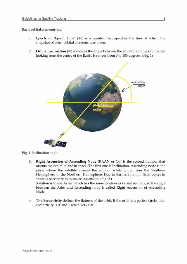
2. Orbital inclination (I0) indicates the angle between the equator and the orbit when looking from the centre of the Earth. It ranges from 0 to 180 degrees. (Fig. 1)
Fig. 1. Inclination angle
3. Right Ascension of Ascending Node (RAAN or O0) is the second number that orients the orbital plane in space. The first one is Inclination. Ascending node is the place where the satellite crosses the equator while going from the Southern Hemisphere to the Northern Hemisphere. Due to Earth's rotation, fixed object in space is necessary to measure Ascension. (Fig. 2.) Solution is to use Aries, which has the same location as vernal equinox, so the angle between the Aries and Ascending node is called Right Ascension of Ascending Node.
4. The Eccentricity defines the flatness of the orbit. If the orbit is a perfect circle, then eccentricity is 0, and 1 when very flat.
www.intechopen.com

Fig. 2. Ascending node's Right Ascension
5. Due to elliptical shape of the orbit, satellite will sometimes be closer and sometimes
further from the Earth. The point where the satellite is closest to the Earth is called Perigee, and the point where it's furthest from the Earth is called Apogee. (Fig 3.)
Fig. 3. Perigee and Apogee
The angle formed between the perigee and the ascending node is called the
Argument of Perigee. The argument of perigee would have the value 0 if the perigee would occur at the ascending node. (Fig. 4.)
www.intechopen.com

Guidelines for Satellite Tracking 5
Fig. 4. Argument of Perigee
6. The Mean Motion is the value that illustrates how fast the satellite is going. According to Kepler's Law:
v2=GM/r
v = velocity of the satellite (m/s) M = Earth's mass (5.98*1024) G = gravitational constant (6.672*10-11 Nm2/kg2) r = distance between the satellite and centre of the Earth (m)
The closer the satellite gets to the Earth, more speed it gets. This value will help us obtain the satellite's altitude.
7. The Mean Anomaly ranges from 0 to 360 degrees, it's referenced to the perigee and represents satellite's position on orbital path. In the perigee itself, mean anomaly would be 0.
8. The Drag is final, optional value that encapsulates atmospheric drag as well as gravitational pull from stellar bodies such as Sun or the moon. Knowledge of the atmospheric density at the satellite’s position is required to calculate the drag force on the satellite. It may also be required in terms of establishing a reliable linkto the satellite. Nevertheless, this may require more information than density alone. (King-Hele, 1983.) Just for density calculations two models should be mentioned. The Harris-Priester model and the Jacchia model (Bindebrink et al., 1989.)
If only gravitational force is assumed by Newton’s law is acting on the satellite the first five parameters are constant and the orbit is an ideal Keplerian orbit (Bunnell, P. 1981.)
Considering the tracking of Earth orbiting objects, institution that has the leading role in providing data related to all satellites in the orbit is NORAD4. NORAD periodically releases
4NORAD – North American Aerospace Defense Command
www.intechopen.com
element sets that, in conjunction with certain models, can be used to track satellites and all other objects. These element sets are periodically refined so as to maintain a reasonable prediction capability. It is very important to emphasize that not just any prediction model will do the job. The NORAD element sets are "mean" values obtained by removing periodic variations in a particular way. In order to obtain good predictions, periodic variations must be reconstructed. Reconstruction is done by prediction model in the exactly the same way they were removed by NORAD. To gain maximum prediction accuracy NORAD element sets must be used with one of the following models:
2.1 SGP/SDP propagation models
SGP propagation model, developed by Hilton and Kuhlman in 1966 is used for near-Earth satellites. This model simplifies drag effect on mean motion by taking it as linear in time. SGP4 model was developed by Ken Cranford in 1970 and is also used for near-Earth satellites. Afterwards SGP4 model was extended with deep-space equations by Hujsak in 1979 so it incorporated gravitational effects of the moon and Sun, sectoral and tesseral Earth harmonics important for calculation of half-day and one-day period orbits. This model was named SDP4 model as for deep-space model. Hoots created SGP8 model in 1980 for near-Earth satellites as a simplification of his own theory that uses same gravitational and atmospheric models as Lane and Cranford but with differential equations integrated in a different manner. As a follow up SDP8 model was formed for deep-space satellites. As previously mentioned the first orbit model was developed in 1966 and used to provide orbital elements in the form of two-line elements. They contain the Keplerian elements (Montenbruck et al., 2000.) inclination i, eccentricity e, right ascension Ω, argument of
perigee and Mean anomaly M0 at epoch time t0. Instead of the semi-major axis a, anomalistic mean motion n0 is used. Modified model SGP4 is used since 1970 for the production of two-line element sets for low-Earth satellites by NORAD. It accounts Earth gravitational field through zonal terms J2, J3, J4 and atmospheric drag (assuming a non-rotating spherical atmosphere) through a power density function. The first step in SGP4 calculation is constants calculation:
3
2
1
o
e
n
ka
(1)
whereas GMke , andG is Newton’s universal gravitational constant.
M = the mass of the Earth on the SGP type “mean” motion at epoch
2322
21
21
1
1cos3
2
3
o
o
e
i
a
k
(2)
oe is the “mean” eccentricity at epoch
www.intechopen.com
Guidelines for Satellite Tracking 7
Ω
M
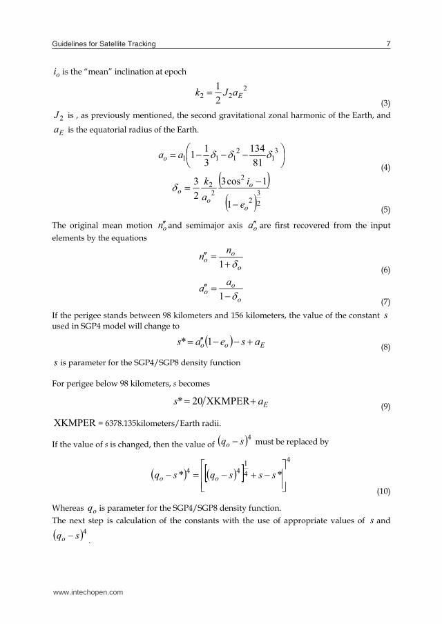
oi is the “mean” inclination at epoch
222
2
1EaJk
(3)
2J is , as previously mentioned, the second gravitational zonal harmonic of the Earth, and
Ea is the equatorial radius of the Earth.
31
2111
81
134
3
11 aao
(4)
2322
2
2
1
1cos3
2
3
o
o
o
o
e
i
a
k
(5)
The original mean motion on and semimajor axis oa are first recovered from the input
elements by the equations
o
oo
nn
1 (6)
o
oo
aa
1 (7)
If the perigee stands between 98 kilometers and 156 kilometers, the value of the constant s
used in SGP4 model will change to
Eoo aseas 1*
(8)
s is parameter for the SGP4/SGP8 density function For perigee below 98 kilometers, s becomes
Eas XKMPER20* (9)
XKMPER = 6378.135kilometers/Earth radii.
If the value of s is changed, then the value of 4sqo must be replaced by
4
4
144
**
sssqsq oo
(10)
Whereas oq is parameter for the SGP4/SGP8 density function. The next step is calculation of the constants with the use of appropriate values of s and 4sqo .
www.intechopen.com
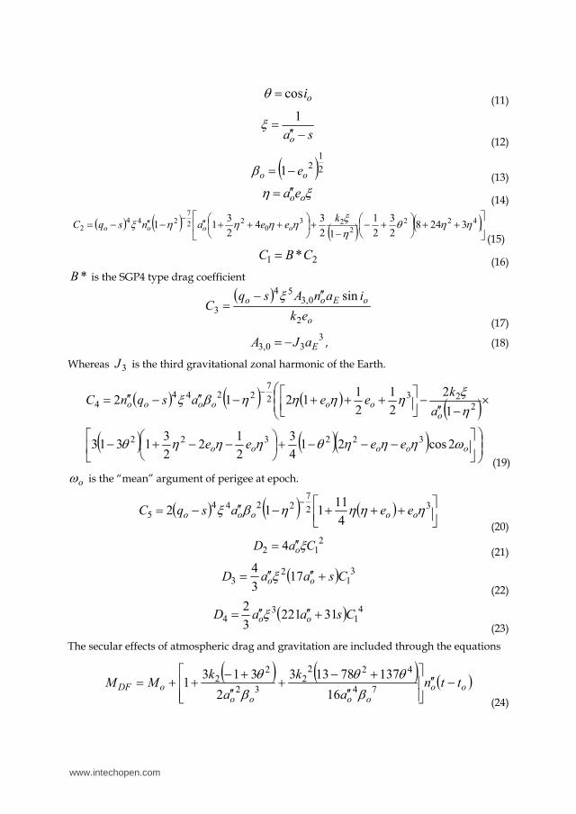
oicos (11)
sao 1
(12)
2121 oo e
(13)
ooea
(14)
422
2
230
22
7244
2 32482
3
2
1
12
34
2
311
keeansqC oooo
(15)
21 *CBC (16)
*B is the SGP4 type drag coefficient
o
oEoo
ek
ianAsqC
2
0,354
3
sin (17)
330,3 EaJA , (18)
Whereas 3J is the third gravitational zonal harmonic of the Earth.
ooooo
o
oooooo
eeee
a
keeasqnC
2cos214
3
2
12
2
31313
1
2
2
1
2
11212
322322
2
232
72244
4
(19)
o is the “mean” argument of perigee at epoch.
32
72244
54
11112 ooooo eeasqC
(20)
212 4 CaD o
(21)
3
12
3 173
4CsaaD oo
(22)
4
13
4 312213
2CsaaD oo
(23)
The secular effects of atmospheric drag and gravitation are included through the equations
oo
oooo
oDF ttna
k
a
kMM
74
4222
32
22
16
13778133
2
3131
(24)
www.intechopen.com
Guidelines for Satellite Tracking 9
B
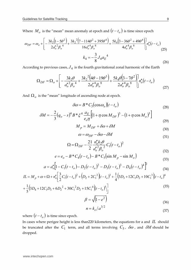
Where oM is the “mean” mean anomaly at epoch and ott is time since epoch
oo
oooooo
oDF ttna
k
a
k
a
k
84
424
84
4222
42
22
4
493635
16
39511473
2
513
(25)
444
8
3EaJk
(26)
According to previous cases, 4J is the fourth gravitational zonal harmonic of the Earth
oo
oooooo
oDF ttna
k
a
k
a
k
84
24
84
322
42
2
2
735
2
19433
(27)
And o is the “mean” longitude of ascending node at epoch.
oo ttCB cos* 3 (28)
3344cos1cos1*
3
2oDF
o
Eo MM
e
aBsqM
(29)
MMM DFp
(30)
MDF
(31)
2122
2
2
21o
oo
oDF ttC
a
kn
(32)
opoo MMCBttCBee sinsin** 54
(33)
244
33
2211 ooooo ttDttDttDttCaa
(34)
5412
21
22314
431213
3212
21
153061235
1
101234
12
2
3
o
oooop
ttCDCDDCD
ttCDCDttCDttCnMIL
21 e
(36)
23
akn e (37)
where ott is time since epoch.
In cases where perigee height is less than220 kilometers, the equations for a and IL should
be truncated after the 1C term, and all terms involving 5C , , and M should be
dropped.
(35)
www.intechopen.com

Add the long-period periodic terms
coseaxN
(38)
1
53cos
8
sin
22
0,3e
ak
iAIL
oL
(39)
2
2
0,3
4
sin
akiA
ao
yNL (40)
LT ILILIL (41)
yNLyN aea sin (42)
Next step involves solving the Kepler’s equation for E by defining
TILU
(43)
iii EEE 1 (44)
1cossin
sincos
ixNiyN
iixNiyNi
EaEa
EEaEaUE
(45)
UE 1
(46)
The following equations are used to calculate preliminary quantities needed for short-period periodics.
EaEaEe yNxN sincoscos (47)
EaEaEe yNxN cossinsin
(48)
2122
yNxNL aae (49)
21 LL eap
(50)
Eear cos1
(51)
Ee
r
akr e sin
(52)
r
pkfr Le
(53)
2
11
sincoscos
L
yNxN
e
EeaaE
r
au
(54)
www.intechopen.com
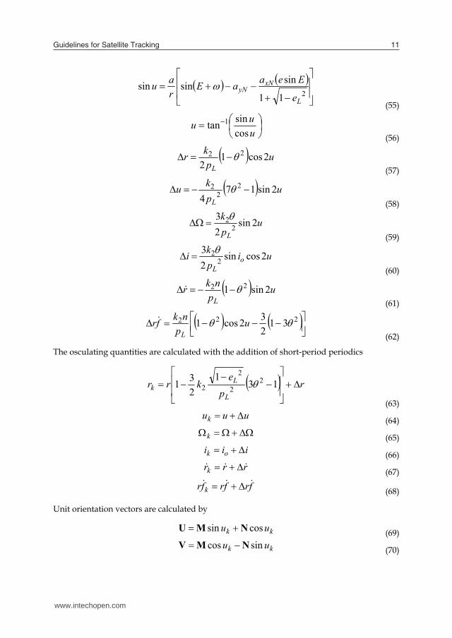
Guidelines for Satellite Tracking 11
2
11
sinsinsin
L
xNyN
e
EeaaE
r
au
(55)
u
uu
cos
sintan
1
(56)
up
kr
L
2cos12
22 (57)
up
ku
L
2sin174
2
2
2 (58)
up
k
L
2sin2
32
2 (59)
uip
ki o
L
2cossin2
32
2 (60)
up
nkr
L
2sin122
(61)
222 31
2
32cos1 u
p
nkfr
L
(62)
The osculating quantities are calculated with the addition of short-period periodics
rp
ekrr
L
Lk
13
1
2
31
2
2
2
2 (63)
uuuk
(64)
k (65)
iii ok
(66)
rrrk
(67)
frfrfr k
(68)
Unit orientation vectors are calculated by
kk uu cossin NMU (69)
kk uu sincos NMV (70)
www.intechopen.com

where
kz
kky
kkx
iM
iM
iM
sin
coscos
cossin
M
(71)
0
sin
cos
z
ky
kx
N
N
N
N
(72)
Then, position and velocity are given by
Ur kr (73)
and
VUr kk frr
(74)
2.2 Propagation models modifications
SGP propagation model was modified in time. Several minor points in the original SGP4 paper emerged where performance of SGP4 could be improved. To maximise the usefulness of all of these features, one should ideally use Two Line Elements formed with differential correction, using an identical model as well (Vallado, D. et al. 2006). Next chapter will shed some light on what Two Line Elements are.
3. Two Line Elements
Orbit tracking programs require information about the shape and orientation of satellite orbits. That information was available from different websites. One of most common quoted sources is CelesTrak.com website, maintained by the group of satellite tracking enthusiasts. As a result of legislation passed by the US Congress and signed into law on 2003 November 24 (Public Law 108-136, Section 913), which was updated in 2006 (US National Archives, 2006.), Air Force Space Command (AFSPC) has embarked on a three-year pilot program to provide space surveillance data—including NORAD two-line element sets (TLEs)—to non-US government entities (NUGE). Since US Public Law prohibits the redistribution of the data obtained from this new NUGE service "without the express approval of the Secretaryof Defence“a lot of other sources were immediately shut down. CelesTrak has received continuing authority to redistribute Space Track data from US government and that way become one of the most useful information sources for the community. TLE’s are redistributed in a form shown in Fig.5. All relevant parameters are color-coded and explained in Table 1.
堅王 堅王
www.intechopen.com
Guidelines for Satellite Tracking 13
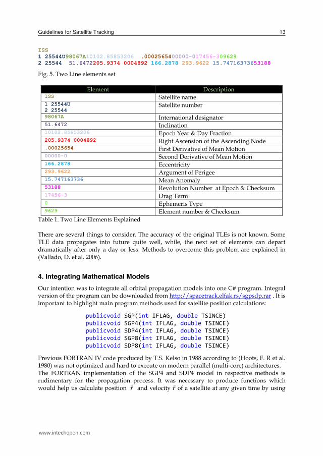
ISS
1 25544U98067A10102.85853206 .0002565400000-017456-309629
2 25544 51.6472205.9374 0004892 166.2878 293.9622 15.74716373653188
Fig. 5. Two Line elements set
Element Description ISS Satellite name 1 25544U
2 25544 Satellite number
98067A International designator 51.6472 Inclination 10102.85853206 Epoch Year & Day Fraction 205.9374 0004892 Right Ascension of the Ascending Node .00025654 First Derivative of Mean Motion 00000-0 Second Derivative of Mean Motion 166.2878 Eccentricity 293.9622 Argument of Perigee 15.747163736 Mean Anomaly 53188 Revolution Number at Epoch & Checksum 17456-3 Drag Term 0 Ephemeris Type 9629 Element number & Checksum
Table 1. Two Line Elements Explained There are several things to consider. The accuracy of the original TLEs is not known. Some TLE data propagates into future quite well, while, the next set of elements can depart dramatically after only a day or less. Methods to overcome this problem are explained in (Vallado, D. et al. 2006).
4. Integrating Mathematical Models
Our intention was to integrate all orbital propagation models into one C# program. Integral version of the program can be downloaded from http://spacetrack.elfak.rs/sgpsdp.rar . It is important to highlight main program methods used for satellite position calculations:
publicvoid SGP(int IFLAG, double TSINCE) publicvoid SGP4(int IFLAG, double TSINCE) publicvoid SDP4(int IFLAG, double TSINCE) publicvoid SGP8(int IFLAG, double TSINCE) publicvoid SDP8(int IFLAG, double TSINCE)
Previous FORTRAN IV code produced by T.S. Kelso in 1988 according to (Hoots, F. R et al. 1980) was not optimized and hard to execute on modern parallel (multi-core) architectures. The FORTRAN implementation of the SGP4 and SDP4 model in respective methods is rudimentary for the propagation process. It was necessary to produce functions which would help us calculate position 堅王 and velocity 堅王 of a satellite at any given time by using
www.intechopen.com
the TLE data. Models specified in (Hoots, F. R. and al., 1980) from the original FORTRAN IV code are ported to C# in respect to the corrections made during the years, especially in the SDP4 subroutine DEEP. C# code contains the same variable names and structures as in the original FORTRAN routines to ensure compatibility and expandability. Additional encapsulation was done with the creation of ActiveX component ready to be integrated in any .NET project.
5. NAVSTAR Satellite Tracking Software
NAVSTAR satellite tracking software presented in this paper is also based on the mathematical SGP4/SDP4 model. Program uses two line elements set as an input to calculate and visualize satellite’s position in Space. It can be used to navigate telescopes to space objects passing over certain point on Earth. The complete mathematical model is encapsulated in ActiveX control, so it acts like a black box. The data is provided from TLEs and on the other end viewport coordinates are calculated. NAVSTAR has three basic functions:
Graphical display of satellite positions in real-time, simulation, and manual modes;
Tabular display of satellite information in the same modes;
Generation of tables (ephemerides) of past or future satellite information for planning or analysis of satellite orbits.
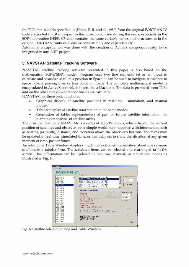
The principal feature of NAVSTAR is a series of Map Windows, which display the current position of satellites and observers on a simple world map, together with information such as bearing (azimuth), distance, and elevation above the observer's horizon. The maps may be updated in real time, simulated time, or manually set to show the situation at any given moment of time, past or future. An additional Table Window displays much more-detailed information about one or more satellites in a tabular form. The tabulated items can be selected and rearranged to fit the screen. This information can be updated in real-time, manual, or simulation modes as illustrated in Fig. 6.
Fig. 6. Satellite selection dialog and Table Window
www.intechopen.com
Guidelines for Satellite Tracking 15
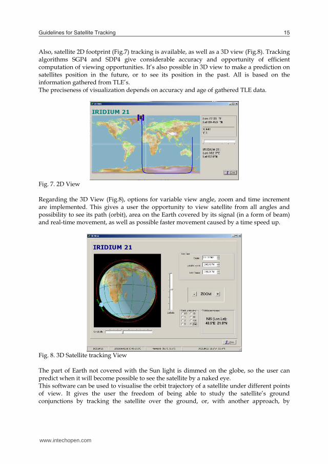
Also, satellite 2D footprint (Fig.7) tracking is available, as well as a 3D view (Fig.8). Tracking algorithms SGP4 and SDP4 give considerable accuracy and opportunity of efficient computation of viewing opportunities. It’s also possible in 3D view to make a prediction on satellites position in the future, or to see its position in the past. All is based on the information gathered from TLE’s. The preciseness of visualization depends on accuracy and age of gathered TLE data.
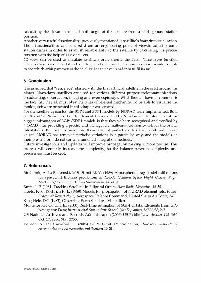
Fig. 7. 2D View Regarding the 3D View (Fig.8), options for variable view angle, zoom and time increment are implemented. This gives a user the opportunity to view satellite from all angles and possibility to see its path (orbit), area on the Earth covered by its signal (in a form of beam) and real-time movement, as well as possible faster movement caused by a time speed up.
Fig. 8. 3D Satellite tracking View The part of Earth not covered with the Sun light is dimmed on the globe, so the user can predict when it will become possible to see the satellite by a naked eye. This software can be used to visualise the orbit trajectory of a satellite under different points of view. It gives the user the freedom of being able to study the satellite’s ground conjunctions by tracking the satellite over the ground, or, with another approach, by
www.intechopen.com
calculating the elevation and azimuth angle of the satellite from a static ground station position. Another very useful functionality, previously mentioned is satellite’s footprint visualisation. These functionalities can be used ,from an engineering point of view,to adjust ground station dishes in order to establish reliable links to the satellite by calculating it’s precise position with the help of TLE data sets. 3D view can be used to simulate satellite’s orbit around the Earth. Time lapse function enables user to see the orbit in the future, and exact satellite’s position so we would be able to see which orbit parameters the satellite has to have in order to fulfil its task.
6. Conclusion
It is assumed that “space age” started with the first artificial satellite in the orbit around the planet. Nowadays, satellites are used for various different purposes:telecommunications, broadcasting, observation, imaging and even espionage. What they all have in common is the fact that they all must obey the rules of celestial mechanics. To be able to visualise the motion, software presented in this chapter was created. For the satellite dynamics, the SGP4 and SDP4 models by NORAD were implemented. Both SGP4 and SDP4 are based on fundamental laws stated by Newton and Kepler. One of the biggest advantages of SGP4/SDP4 models is that they’ve been recognized and verified by NORAD thus providing a precise and manageable mathematical framework for the orbital calculations. But bear in mind that those are not perfect models.They work with mean values. NORAD has removed periodic variations in a particular way, and the models, in their present form do not contain numerical integration methods. Future investigations and updates will improve propagation making it more precise. This process will certainly increase the complexity, so the balance between complexity and preciseness must be kept.
7. References
Binderink, A. L.; Radomski, M.S.; Samii M. V. (1989) Atmospheric drag model calibrations for spacecraft lifetime prediction; In NASA, Goddard Space Flight Center, Flight Mechanics/ Estimation Theory Symposium; 445-458
Bunnell, P. (1981) Tracking Satellites in Elliptical Orbits; Ham Radio Magazine; 46-50. Hoots, F. R.; Roehrich R. L. (1980) Models for propagation of NORAD element sets; Project
Spacecraft Report No. 3; Aerospace Defence Command, United States Air Force, 3-6 King-Hele, D.G (1983), Observing Earth Satellites, Macmillan Montenbruck, O.; Gill, E.. (2000) Real-Time estimation of SGP4 Orbital Elements from GPS
Navigation Data; International Symposium SpaceFlight Dynamics, MS00/28; 2-3 US National Archives and Records Administration.(2006) US Public Law, Section 109–364;
Oct. 17, 2006, Stat. 2355. Vallado A. D.; Crawford P. (2006) SGP4 Orbit Determination; American Institute of
Aeronautics and Astronautics publication; 19-21.
www.intechopen.com

Satellite CommunicationsEdited by Nazzareno Diodato
ISBN 978-953-307-135-0Hard cover, 530 pagesPublisher SciyoPublished online 18, August, 2010Published in print edition August, 2010
InTech EuropeUniversity Campus STeP Ri Slavka Krautzeka 83/A 51000 Rijeka, Croatia Phone: +385 (51) 770 447 Fax: +385 (51) 686 166www.intechopen.com
InTech ChinaUnit 405, Office Block, Hotel Equatorial Shanghai No.65, Yan An Road (West), Shanghai, 200040, China
Phone: +86-21-62489820 Fax: +86-21-62489821
This study is motivated by the need to give the reader a broad view of the developments, key concepts, andtechnologies related to information society evolution, with a focus on the wireless communications andgeoinformation technologies and their role in the environment. Giving perspective, it aims at assisting peopleactive in the industry, the public sector, and Earth science fields as well, by providing a base for their continuedwork and thinking.
How to referenceIn order to correctly reference this scholarly work, feel free to copy and paste the following:
Dusan Vuckovic, Petar Rajkovic, Dragan Jankovic and Olivera Pavic (2010). Guidelines for Satellite Tracking,Satellite Communications, Nazzareno Diodato (Ed.), ISBN: 978-953-307-135-0, InTech, Available from:http://www.intechopen.com/books/satellite-communications/guidelines-for-satellite-tracking

© 2010 The Author(s). Licensee IntechOpen. This chapter is distributedunder the terms of the Creative Commons Attribution-NonCommercial-ShareAlike-3.0 License, which permits use, distribution and reproduction fornon-commercial purposes, provided the original is properly cited andderivative works building on this content are distributed under the samelicense.