Guideline and standards for tTEM data collection

G

uideline and standards for tTEM data collection, processing, and inversion - H

GG

- Aarhus U

niversityGuideline and standards for tTEM data collection, processing, and inversionVersion 1.1 - November 2020

Version 1.1, November 2020

HydroGeophysics Group Department of Geoscience, Aarhus University, Denmark

Guideline and standards for tTEM data collection, processing, and inversion

1

TABLE OF CONTENTS

1 Revision history ................................................................ 3

2 Introduction ...................................................................... 4

3 The tTEM-system, data collection, and data formats ......... 6

3.1 The tTEM-system 6

3.2 Survey planning and navigation 8

3.3 Data Formats 11

4 Instrument validation/Calibration .................................. 17

4.1 Pre-survey calibration/validation 17

4.2 Daily Instrument/data Validation 20

5 Data processing .............................................................. 22

5.1 Data import - convolution, uncertainty estimation 22

5.2 GPS-processing 23

5.3 db/dt data processing 23

6 Inversion ......................................................................... 29

7 Reporting ........................................................................ 31

7.1 Geophysical survey report 31

7.2 Reporting to GERDA 32

8 FloaTEM .......................................................................... 33

9 References ...................................................................... 36

Appendix 1 Documentation of the GEX filE

2

Main Authors

Ph.D. Nikolaj Foged,

Ph.D., Associate Prof. Anders Vest Christiansen.

Aarhus University, Department of Geoscience, HydroGeophysics Group,

Aarhus, Denmark, August 2020.

This Guideline and standards for tTEM data collection, was prepared within the

framework of GeoFysikSamarbejdet (GFS), which is a collaboration between

The Danish Environmental Protection Agency and the HGG at Department

of Geoscience, Aarhus University.

Acronyms

Acronyms

AEM Airborne ElectroMagnetics

ATV All-Terrain Vehicle (quad bike)

DOI Depth of Investigation

EM-methods Electromagnetic methods which induce electrical currents in the ground through the principle of electromagnetic induction

GFS GeoFysikSamarbejdet, collaboration between The Danish Environmental Protec-tion Agency and the Department of Geoscience, Aarhus University

HGG The HydroGeophysics Group at the Department of Geoscience, Aarhus University

LCI Laterally Constrained Inversion

SCI Spatially Constrained Inversion

TEM Transient Electromagnetic

tTEM Towed TEM

UTC Coordinated Universal Time

QC Quality Control

3

1 REVISION HISTORY

The latest version of this guide is available on the web page of the HydroGe-

ophysics Group: www.hgg.au.dk

Version 1.0 - September 2020

This is the first version of the Guideline and standards for tTEM data collection,

processing, and inversion. This version of the guide reflects the present stage of

the tTEM-system, the processing software, and the inversion algorithms.

(August 2020).

The tTEM guideline report version 1.0 was reviewed by Miljøstyrelsen (The

Danish Environmental Protection Agency) prior to release.

Version 1.1 – November 2020

Minor edits in section 4.1 and 4.2 regarding temperature variations in the

tTEM transmitter unit.

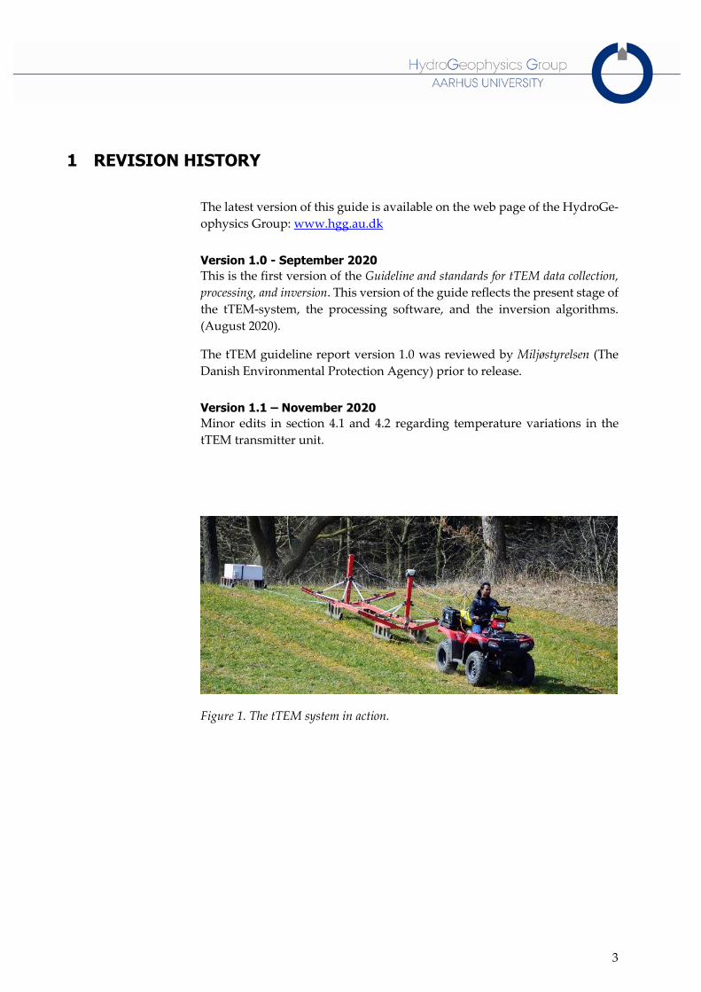
Figure 1. The tTEM system in action.

http://www.hgg.au.dk/

4

2 INTRODUCTION

The tTEM system is a compact, highly efficient, towed TEM-system, de-

signed for detailed 3D geophysical mapping of the shallow subsurface, ap-

proximate 0-80 m. The purpose of this guide is to ensure uniform and high

quality standards for the tTEM data collection, the data processing and in-

version, and the survey reporting, but this guide also serves as a description

of the workflow as well as documentation for the data formats of the tTEM

system.

The standards presented here are aligned to standards and requirements set

to other geophysical data collected for hydrogeological mapping in Den-

mark. In general, despite the Danish context of this guide, the guide provides

a review of the different steps in a tTEM mapping campaign in regard to

workflow, quality control, data processing, and inversion.

The following describes the three roles in a tTEM survey:

Instrument Owner: The company/institution that owns the tTEM in-

strumentation and rents it out for tTEM surveys.

Contractor: The person(s)/company that performs the data collection

(operates the tTEM system) and performs the data processing/inver-

sion and reporting to the Client. Typically, a consultant company.

Client: The company/institution that ordered the tTEM survey and

receives the survey reporting and the mapping results, e.g. The Dan-

ish Environmental Protection Agency or a water plant.

Requirements in this guide will be referenced to one of the three defined

roles. In this guide it is assumed that data collection, processing, and inver-

sion is carried out by the same contractor and that required documentation

of the different steps is incorporated in a survey report to the client.

In case the requirements cannot be met, the reasons for this must be stated

clearly in the final report and, where relevant, the involved parties must be

informed in time. It is required that the contractor and client have open and

frequent dialogues about important irregularities or issues during mapping

and data processing.

The guide provides a number of typical/recommended processing and inver-

sion settings. The typical/recommended processing and inversion settings

are not requirements, and the settings must be adjusted to the specific sur-

vey/target.

It is assumed and recommended that data processing and inversion is con-

ducted with the Aarhus Workbench software, since Aarhus Workbench

holds modules specific designed for tTEM data processing, inversion, and

5

data upload to the Danish National geophysical database. Thus, this guide

holds direct references to specific Aarhus Workbench processing and inver-

sion settings. Also, general experience and knowledge of TEM data collec-

tion, processing, and inversion is assumed. Thus, this guide is not a training

guide or an operation manual for the tTEM instrument and data processing.

The tTEM system also comes in a FloaTEM version, operated on water. Sec-

tion 8 holds details and additional requirements for the FloaTEM system.

The Notes provided in the sections are primarily guides/hints to specific set-

tings or steps in the workflow.

References for this guide are grouped under the different topics in the refer-

ence section (9), with no direct references in the text.

6

3 THE TTEM-SYSTEM, DATA COLLECTION, AND DATA FORMATS

In the following sections we present the tTEM system, provide recommenda-

tions regarding survey planning and data collection, and provide documen-

tation of the different tTEM data formats.

3.1 THE TTEM-SYSTEM

The tTEM-system is a towed, ground-based, transient electromagnetic sys-

tem, designed for highly efficient data collection and detailed 3D-mapping of

the shallow subsurface (the upper ~80 m). The present layout of the tTEM

system is shown in Figure 1 and Figure 2. The main development of the

tTEM-system was conducted in 2016-2018, building on the high expertise and

experience within the HGG-group regarding all aspects of the TEM-method:

from instrument design, testing and calibration, to data surveying, pro-

cessing, and inversion of EM-data.

The tTEM-system (Figure 2) consists of an ATV carrying the instrumentation

and towing the transmitter frame (Tx coil) and the receiver coil (Rx coil) in an

offset configuration. The Tx and Rx coils are mounted on sleds for a smooth

ride over rough fields/terrain. The frame and sleds are built of non-electri-

cally conductive fiberglass and composite materials and are assembled with

3D printed, carbon-strengthened, parts.

Figure 2. Schematic layout out of the tTEM system (2020).

The operational speed of the tTEM system is up to 20 km/h and depending

on terrain and surface conditions the actual speed will vary accordingly.

When surveying on farmland, the service tracks in the fields are used as driv-

ing guides to minimize crop impact. The production rate strongly deepens

on: Line density, condition of the fields, field sizes, and accessibility/connec-

tivity of the fields. The production rate, therefore typically spans from 50-250

hectares/day (0.5-2 km2/day).

7

Navigation and data collection are monitored and controlled by the driver

using a tablet PC. The navigation software (Aarhus Navigator) provides a

real time display of the survey path, line numbers, status parameters, and

various alarms from the instrumentation. Pre-planned survey lines and GIS

maps can be loaded into the navigation system. The geographical position of

the data is recorded by one SBAS (Satellite Based Augmentation System) GPS

placed on the Tx-frame. In the later data processing, the GPS data are lag-

corrected to position the data/resistivity model at the midpoint between the

transmitter and receiver loops.

The tTEM system is operated by one person, but a second person is required

for mobilization/demobilization, on-site survey planning, data quality con-

trol, and field safety. Mobilization as well as demobilization is quite fast and

takes approximately 20 min. Transportation wise, the 2 x 4 m2 frame fits on a

long car trailer. Placing the ATV in the back of the van makes transportation

a single car job. Additionally, the system can be disassembled and palletized

for longer transportation and shipment.

Figure 3. The tTEM system packed on the transport trailer. The ATV and all instru-

mentation fit inside the van.

8

3.2 SURVEY PLANNING AND NAVIGATION

A tTEM survey requires ground access, and the ground surface needs to be

drivable for the ATV towing the tTEM system. Most often, there will be sub-

areas in the survey region that cannot be mapped due to lack of access per-

mission or non-drivable ground. This could be wet meadow areas, forest ar-

eas or farmland with (too much) livestock. Even if a dense mapping cannot

be obtained in some subareas, it will, most often, be beneficial to have a few

scattered lines in these areas e.g. obtained by driving on small pathways in

forest areas or similar.

It is preferable that a survey is carried out in one continuous campaign, since

seasonal variations in the resistivity of the shallow layers cannot be ruled out.

Line spacing and resolution

The footprint of the tTEM system is quite small in the top ~20 meters com-

pared to other TEM systems, and it is recommended to aim for a general line

spacing of maximum 25 m. A line spacing of less than 10 m will not increase

the resolution due to the footprint size. Depending on the target and pur-

poses of the mapping, the line spacing must be set accordingly.

Before the survey, client and contractor agree on a target line spacing, and

since the distance between the service tracks in some cases dictates the line

spacing, moderate deviations from the target line spacing must be expected.

Survey layout

In the tTEM navigation program, Aarhus Navigator, you can upload pre-pre-

pared driving routes, with the desired line spacing to follow during the data

collection. This approach is mainly useful if you have open land where you

are free to drive anywhere.

When mapping in farmland areas, the normal approach is to map the survey

area field by field and it is good practice (sometimes a demand from the

farmer) to use the service tracks in the fields. In this case the line spacing is

limited to the distance between service tracks or multiples thereof. Figure 4

shows an example of mapping in a farmland area.

9

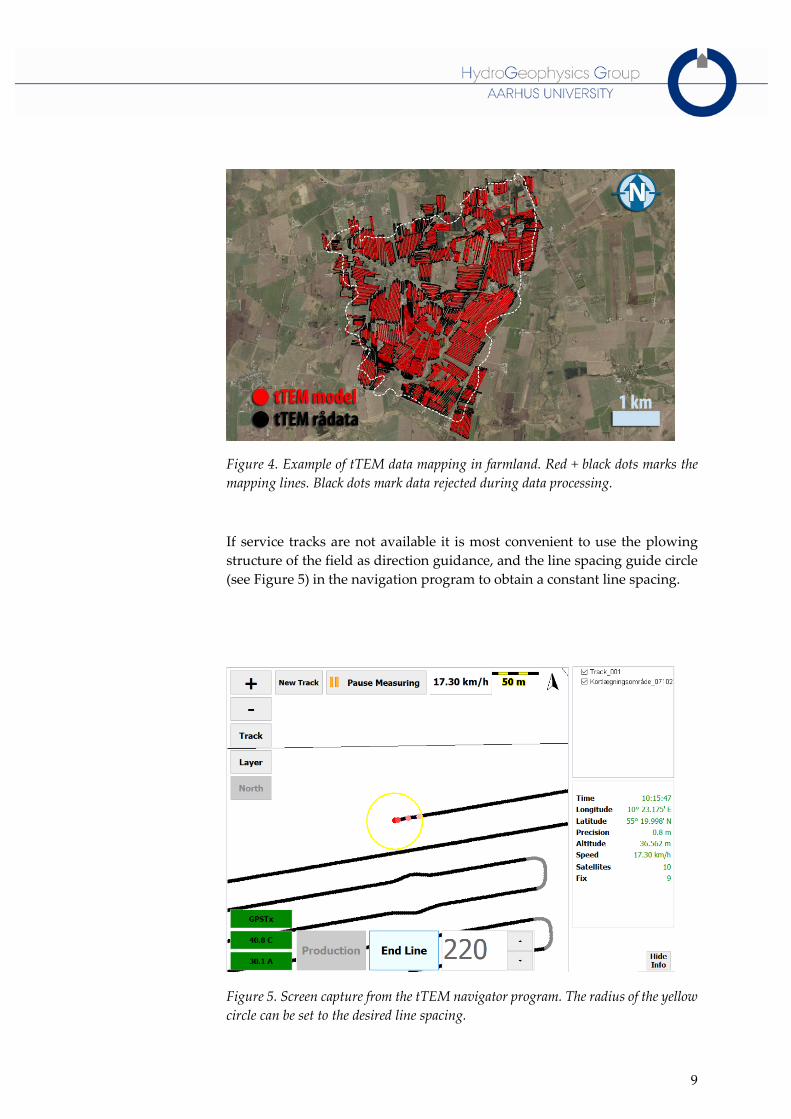
Figure 4. Example of tTEM data mapping in farmland. Red + black dots marks the

mapping lines. Black dots mark data rejected during data processing.

If service tracks are not available it is most convenient to use the plowing

structure of the field as direction guidance, and the line spacing guide circle

(see Figure 5) in the navigation program to obtain a constant line spacing.

Figure 5. Screen capture from the tTEM navigator program. The radius of the yellow

circle can be set to the desired line spacing.

10

Driving speed

The driving speed should be kept fairly constant. An uneven driving speed

will result in an uneven spacing of the resistivity models along the lines, since

data are stacked in equidistant time intervals. The normal target speed is 20

km/h for the tTEM system, and one should not exceed a driving speed of 25

km/h for safety reasons and to limit vibration noise. In noisy areas (highly

resistive areas), it can be beneficial to lower the speed to increase the data

stack, especially if the focus is on deep mapping. On rough terrain, the speed

should be adjusted accordingly to minimize vibrational noise and to ensure

instrumentation/driving safety. In case of rough terrain, on small forest trails

etc. the mapping speed will often be reduced to 5-10 km/h. Reducing the

speed might also be needed in forest areas to obtain a good GPS-signal.

Line shift - start/end line procedure

It is important that the rope between the transmitter coil and the receiver coil

is fully extended, as a constant distance between transmitter and receiver coil

is assumed in the modeling of the data. Furthermore, the ATV will cause dis-

tortion in the data if it is too close to the transmitter/receiver coils. At U-turns

(when shifting lines) the system operator must give an ‘End Line’ indication

in the navigation program (see Figure 5) when the turning starts. It is equally

important that the ‘Production’ (start line) indication for the next line is not

given before the towing rope is fully stretched and the transmitter and the

receiver are aligned. Data between an ‘End Line’ and the next ‘Production’ in-

dication are automatically removed in the later data processing. Missed End

line/Production marks can normally, be corrected manually in the later pro-

cessing, since data are recorded/saved no matter which Production/End of line

state the instrument is set for. If a stop on a line is needed, the operator must

give an End line mark.

With a total system length of ~15 m, some data loss at the beginning and end

of the fields/lines is unavoidable. Furthermore, when operating in service

tracks the line turning will normally start 10-15 m before the end of the field

where the farmer also makes turns with his farm machinery. A skilled U-

turning technique, by overshooting the turn slightly, will result in a quicker

alignment of the system and less data loss when turning.

In general, it is preferable to drive in straight lines. Smooth changes in driving

direction can be conducted without initiating the described end/begin line

procedure, and it is acceptable that the receiver coil slides ~1 meter from side

to side while driving.

Measurement script

The measurement script controls the repetition frequency, the low mo-

ment/high moment (LM/HM) cycle, key data normalization factors, etc. The

11

measurement script must be designed to stack out the power line frequency

noise (50/60 Hz).

Note:

Noise measurements (transmitter off) are normally not included in

the measurement scripts.

Change of system components might require adjustment in the meas-

urement script.

3.3 DATA FORMATS

This section describes the output files from the instrument and additional

setup files required to perform the data processing in Aarhus Workbench.

This section also serves as documentation for the different file formats, thus

a high level of detail in this section.

Instrument output files:

Line number file

Rwb file

SPS files (two types)

Instrument modeling and setup files

System geometry file

Filter file

Line number file (*.lin)

The line number file holds the production time intervals associated with a

line number, a line type, start/end UTM position of each line, and an optional

comment. Only data within the specified time intervals in the line number

files are imported in the processing software. The Line number file is created

during data acquisition, based on the system operator’s begin/end line indi-

cations as described in section 3.2. Figure 6 holds an example of a part of a

line file.

12

Each tTEM-line is defined by two text lines (start and end) in the file. The line

number increment is +10 starting from line number 100, hence the order of

the line numbers reflects the data recording order. The operator can set the

line number manually in the field at the start of each line or make corrections

directly in the line file post survey. A more geographically based ordering of

the line number naming is preferable, but at present, no automatic line file

un-scrambler routine/software exists.

The automatically generated comments indicate if data are Testpoints or Pro-

duction. The Testpoints/Production stage is set by the operator during the data

collection and serves only as a bookkeeping tool; no automatic filtering with

respect to the Testpoints/Production comment is performed in the later data

processing.

RWB files (*.RWB)

The RWB-file is the tTEM-instrument output file containing the TEM data

(the db/dt responses) in a binary format. The RWB-file holds an Ascii header,

which is an exact duplicate of the system configuration, holding information

about measuring scheme, amplification, gating, etc. (copy of script.idx,

script.ini). Under no circumstances should changes be made to the ascii

header of the RWB-files, since these settings represent how data were rec-

orded.

The RWB-file names are date-time tagged (UTC time) and a new RWB-file is

created when the data recording program (PaPC) is started and at any instru-

ment re-starts.

Aarhus Workbench is compatible with the RWB-file format.

GPS-file (*NavTTem.sps)

The NavTTem sps-files hold the GPS-data. Figure 7 shows four GPS-lines

from a NavTTem.sps files. Only lines starting with G12 in the file are used.

Date Time Line UtmX UtmY DataFolder Comment

27-03-2020 10:53:31 20000 503789.31 6283318.81 !Run1 "TestPoint, start"

27-03-2020 10:53:47 20000 503789.32 6283318.81 !Run1 "TestPoint, end"

27-03-2020 11:09:20 100 503820.19 6283310.34 !Run3 "Production, start"

27-03-2020 11:10:06 100 503959.47 6283324.15 !Run3 "Production, end"









Figure 6 Line file example. Blue header text is not part of the file.

13

.

The explanation of the G12 line is given in the table below.

Colum GPS-devise

1 GPS sting type: G12

2-8 UTC, [yyyy mm dd hh mm ss zzz]

9 Standard $GPGGA string. http://aprs.gids.nl/nmea/#gga for detailed info.

9AB Latitude and longitude coordinates in Degrees Minutes DecimalMinutes [degmm.mm]. EX: 5640.0122390 = 56° 40.0122390 minutes

10 Standard $GPVTG string. http://aprs.gids.nl/nmea/#vtg for detailed info.

Table 1 Explanation of the columns of the NavTTem sps-files in Figure 7.

The GPS data is an essential part of the tTEM-data set, and GPS dropouts of

more than ~4 s will result in data loss in the later processing.

TX-current (*_PaPc.sps)

The transmitter current is measured for each transient and stored for each

HM and LM data sequence in the PaPC.sps file. The PaPC.sps also holds a

number of transmitter status/QC parameters like temperature and battery

voltage.

Figure 8 shows eight lines of a PaPC.sps file with the parameter explanation

in Table 2. Note is it only the Mean current (column 20, see Table 2), that is

used in the data processing for data normalization.

1 2 3 4 5 6 7 8 9 9A 9B 10 G12 2020 06 10 08 57 04 655 $GPGGA,085705.20,5627.3624751,N,00940.6469218,E,2,18,0.6,9.087,M,39.291,M,,*66;$GPVTG,0.00,T,,,0.01,N,0.03,K,D*77;

G12 2020 06 10 08 57 04 858 $GPGGA,085705.40,5627.3624748,N,00940.6469230,E,2,18,0.6,9.077,M,39.291,M,,*6D;$GPVTG,0.00,T,,,0.02,N,0.03,K,D*74;

G12 2020 06 10 08 57 05 061 $GPGGA,085705.60,5627.3624747,N,00940.6469232,E,2,18,0.6,9.073,M,39.291,M,,*66;$GPVTG,0.00,T,,,0.02,N,0.03,K,D*74;

G12 2020 06 10 08 57 05 249 $GPGGA,085705.80,5627.3624758,N,00940.6469167,E,2,18,0.6,9.075,M,39.291,M,,*63;$GPVTG,0.00,T,,,0.03,N,0.06,K,D*70;

Figure 7 NavTTem sps-files example. Blue header text is not part of the file. See Table 1 for explanation.

http://aprs.gids.nl/nmea/#gga

http://aprs.gids.nl/nmea/#vtg

14

Row Transmitter, TXD-devise

1 Device type [TXD]

1-8 UCT-PC-time, [yyyy mm dd hh mm ss zzz]

9 NumberOfShots: The total number of LM or HM transients

10 NumberOErrors: Indicates a missing pulse detection. The integer states the num-ber of missing pulses.

11 FirstProtemError: The position of the first missing pulse.

12 Nplus: The number of positive currents in stack.

13 Nminus: The number of negative currents in stack.

14 VoltageOn: The battery voltage measured during transmitter on time, [V].

15 VoltageOff: The battery voltage measured during transmitter off time, [V].

16 TxTemperature: The temperature of the transmitter, [°C].

17 VersionNo: Added to be able to add new elements to the frame. VersionNo 0 is without PolErr and VersionNo1 is with PolErr. VersionNo 3 adds Max_Current, Min_Current and RMS_Current.

18 NumberOfDatasets: The number of data sets.

19 NumberOfSeries: The number of series in each data set.

20 Mean_Current: The mean transmitter current for NumberOfSeries. Measured for before the ramp off, [A].

21 Max_Current: Not in use

22 Min_Current: Not in use

23 RMS_Current: Not in use

Table 2. Explanation of the columns of the PaPC sps-files in Figure 8.

1 2 3 4 5 6 7 8 9 10 11 12 13 14 15 16 17 18 19 20 21 22 23

TXD 2020 04 01 07 56 09 900 422 0 0 211 211 0.01 0.01 33.86 0 1 422 5.27 0.00 0.00 0.00

TXD 2020 04 01 07 56 09 900 252 0 0 126 126 0.01 0.01 34.53 0 1 252 30.27 0.00 0.00 0.00

TXD 2020 04 01 07 56 10 500 422 0 0 211 211 0.01 0.01 34.05 0 1 422 5.27 0.00 0.00 0.00

TXD 2020 04 01 07 56 10 500 252 0 0 126 126 0.01 0.01 33.56 0 1 252 29.85 0.00 0.00 0.00

TXD 2020 04 01 07 56 11 100 422 0 0 211 211 0.01 0.01 33.19 0 1 422 5.27 0.00 0.00 0.00

TXD 2020 04 01 07 56 11 100 252 0 0 126 126 0.01 0.01 34.23 0 1 252 29.98 0.00 0.00 0.00

TXD 2020 04 01 07 56 11 700 422 0 0 211 211 0.01 0.01 33.74 0 1 422 5.27 0.00 0.00 0.00

TXD 2020 04 01 07 56 11 700 252 0 0 126 126 0.01 0.01 32.82 0 1 252 30.02 0.00 0.00 0.00

Figure 8. Part of PaPC.sps file. Blue header text is not part of the file. See Table 1 for explanation.

15

The system geometry file (GEX-file)

The GEX-file contains essential information about the specific tTEM sys-

tem/configuration, which is required in the data processing and inversion in

Aarhus Workbench. Below the main content of the GEX-file is listed, while

appendix 1 provides a complete documentation of the GEX-file.

The geometry file contains information about:

The x,y position of the devices and transmitter/receiver coils as

shown in Figure 9. The x,y origin is defined at the center of the trans-

mitter coil. The z-axis is zero ground level and positive downwards.

This results in the z-coordinates in the GEX-file being negative for

coils and devices.

The nominal transmitter current.

The size and area of the transmitter coil and number of turns.

Calibration constants in the form of time shift and db/dt factors

Specification of the first usable gates of each channel

Low-pass filters

The front gates time. The front gate must occur a minimum of 1 µs

before the first usable gate opens.

Parameters describing the transmitter waveform (the turn-off time

before the front gate time).

A uniform data uncertainty. As standard, 3% is used.

Gate center times, gate factors, and gate opening and closing times.

The instrument owner must provide the GEX-file with the instrument, while

the operator must QC and update the GEX-file if needed.

Figure 9. tTEM configuration, coordinate orientation.

16

The filter file (*.TFI)

During import, the data is convolved with a filter that removes 50/60 Hz noise

and DC offset and reduces the vibration noise. The filter also includes a low-

pass filter. A filter for both LM and HM is stated in the filter file (see example

in Figure 10). The Instrument owner provides the filter file.

[FilterSwCh1] /LM

Periodtime = 4.740e-04 /Period time

Filter = 4.79644195210675e-5 3.66167329277456e-5 -5.20872599689183e-5 … /Filter coefficients

[FilterSwCh2] /HM

Periodtime = 1.587e-03 /Period time

Filter = -5.73009583716962e-6 2.13149258960294e-5 1.30906210105234e-4 … /Filter coefficients

Figure 10. Filter file example. Normally the filter holds 50 filter coefficients. Text in blue is not

part of the filter file.

17

4 INSTRUMENT VALIDATION/CALIBRATION

This section concerns instrument calibration and validation to ensure a high

and uniform data quality.

In the tTEM design phase, the system geometry, the position of the instru-

mentation and devices, the cabling and rigging, etc. were carefully designed

and tested to ensure an acceptable system noise/bias level. Therefore re-rig-

ging, changing of the cabling, or the positioning of the instrumentation/de-

vices etc. of the tTEM-system should not be carried out without expert

knowledge and potential re-testing/calibration.

Results of some of the general system validation tests and a comprehensive

validation from the national TEM test site are found in the reference list listed

under TEM-test site calibration and validation.

4.1 PRE-SURVEY CALIBRATION/VALIDATION

TEM test-site calibration

The objective of calibrating the tTEM system at the National TEM test site

near Aarhus is to establish the absolute data level to facilitate precise data

modelling.

The general test site calibration procedure is descried in Foged et.al, 2013. The

following guidelines are set for the tTEM calibration, calibration frequency,

etc.:

The tTEM system must be configured as in production mode for the

calibration measurement.

The tTEM receiver coil is positioned in the center of the TEM test site

with the transmitter south of the receiver coil.

Calculation of the tTEM specific reference response from the refer-

ence model must be with the exact same system parameters (the GEX-

file settings) that are to be used in the later modeling of the data, ex-

cept for the calibration parameters to be obtained.

After calibration, the measured tTEM response must match the refer-

ence response within 5% (late time apparent resistivity data transfor-

mation) for low noise time gates.

The obtained calibration parameters are valid for a specific transmit-

ter instrument using a specific receiver coil type.

Documentation of the calibration is provided in the form of plots

showing the match between the reference response and the measured

data.

18

Instrument calibration based on test site measurements must be per-

formed in the period between fourteen days before/after the survey

period.

For multi day surveys instrument stability is documented by:

o Test site measurements/calibration before and after the sur-

vey, resulting in consistent calibrations parameters.

and/or

o By obtaining consistent data responses from repeating meas-

urements at a local site inside the mapping area.

For single day surveys the initial calibration at the test site is suffi-

cient.

In connection with instrument reconfiguration/adaptation a new test

site calibration is required.

Transmitter Waveform

The transmitter waveform describes how the current ramps up and down in

the transmitter coil and needs to be known in detail for precise modeling of

the data. The tTEM system facilitates an accurate temperature and current

regulation, which results in a constant transmitter waveform within the

needed modeling precision. The tTEM transmitter waveform can therefore

be measured once in detail for a given tTEM system.

The transmitter waveform can be split up in a turn-on and a turn-off part.

The turn-on part is relatively slow and can be measured directly as the cur-

rents flow in the transmitter coil. The turn-off part takes only a few microsec-

onds and needs to be measured with a device capable of sampling the signal

fast enough—typically a small pickup coil measuring the time derivative of

the current in the transmitter loop is used.

Guidelines for the waveform measurement:

The system must be configured as in production mode, though the

ATV and the receiver coil can be omitted.

Separated waveform measurements for turn-on and a turn-off part,

and the LM and HM are performed.

The measured waveforms are approximated with a number of linear

segments to be used for the data modeling.

The resulting waveforms, stated in the GEX-file, must include both a

negative and a positive waveform, separated with the correct period

of time and normalized to a peak amplitude of -1, 1.

The determination of the waveform is documented with plots of the

measured waveforms and the segmented waveforms used in the

GEX-file.

19

The measured waveform is specific for a given tTEM transmitter in-

strument, output current, and transmitter loop.

ATV distance test

The tTEM frame and sleds are built of non-conductive components to avoid

coupling and bias signals. The ATV with the instrumentation is therefore

placed ~3 m away from the front of the transmitter frame to minimize inter-

ference. The tTEM system has been operating with different ATVs and no

issues with the 3 m ATV distance has been observed for any of the different

brands of ATVs. If other types of pulling vehicles than an ATV is used, or by

any doubt of possible interference from the ATV, we recommend that the

ATV test described below is conducted. The ATV test should be conducted

where the earth signal is low (resistive ground) since minor ATV interference

is only detectible in this case.

ATV test procedure:

1. Set up the system as normal, but place the instruments, in the normal

layout, on the ground or on plastic boxes at the end of the towing

rope, instead of on the back of the ATV.

2. Important: Make sure that the transmitter and receiver cables are sep-

arated by a minimum of ~40 cm as when the instruments are mounted

on the ATV.

3. Move the ATV far away (>30 m) and record one minute of data. Make

a note of the line number/time interval. This is the Baseline response.

4. Move the ATV as close to the front of the transmitter frame as possi-

ble (0 m separation). Change the line number and record for one mi-

nute in this position with the ATV engine on.

5. Move the ATV in steps of ~1 m away from the transmitter front to-

wards the instrument boxes and record one minute of data at each

ATV location and note line number, time, ATV separation at each po-

sition. Continue this procedure until the ATV is ~5 m away from the

transmitter front. Remember to make a measurement at the normal

ATV position.

6. End the sequence as stated with the ATV far away.

7. Import the data to Aarhus Workbench. Set the stack width to 40 s and

turn off filters that eliminate data.

8. Plot the stacked data curve (AVE data) at the center time of the time

interval for each ATV distance and compare them with the base line

measurements.

9. You should observe that when the ATV is close to the frame the curve

is disturbed, compared to the base line response.

10. If no systematic dissimilarities between the response at the normal

ATV distance (and longer distances) and the base line response are

20

observed, the ATV - TX-coil distance is sufficient for the specific ATV.

You can evaluate the natural fluctuations of the TEM response by

comparing the start and end baseline responses. Do not shorten the

ATV-transmitter frame distance even if your test results show it is

possible.

4.2 DAILY INSTRUMENT/DATA VALIDATION

This section deals with instrument and data QC conducted in the survey pe-

riod and is performed by the instrument operator.

System geometry

The system geometry: TX-RX distance and TX and RX heights above the sur-

face are used in the later modeling of the data and are therefore needed. The

skids on the sleds are gradually worn down, changing the height of the TX

and RX coils. Also, the TX-Rx distance may change over time, especially if the

towing ropes are repaired or replaced. It is therefore important to check the

system geometry regularly, at least at the start and end of a survey, and when

the towing ropes or skids are replaced or repaired.

The RX-TX distance and the RX and TX heights stated in the GEX-file must

be within +/- 2 cm of the actual geometry. If this is not possible throughout

the survey, the dataset must be split up and assigned different geome-

try/GEX-files accordingly. Minor variation of the distance to the ATV is of no

importance.

The geometry measurements are carried out with the system standing on a

smooth horizontal surface. The coil heights are measured from the ground to

the vertical center of the coil. The RX-TX distance is the horizontal center-to-

center distance of the coils. It is most accurate to measure the RX-TX distance

from the back edge of the transmitter coil to the front edge of the receiver coil

and then add half the coil widths to get the center-to-center distance.

Data QC

On a daily basis, QC of the data normally includes checks of:

Stable transmitter current, at the same level as for the measured

waveform.

Transmitter temperature

Stable GPS signal/data

Correct production intervals (Begin/end line marks)

dB/dt data appear normal and are present where mapped

Real time inversion results look plausible (if performed)

21

Some of these parameters can be followed in real time in the navigator pro-

gram while mapping, and the navigator program gives various alarms in case

of irregularities in the different data streams.

22

5 DATA PROCESSING

In the following, the overall requirements to data processing are outlined.

The data processing is performed in the tTEM processing module of the Aar-

hus Workbench.

Generally, the following should be performed in the processing of the tTEM

data.

Review of the test site calibration

Review of the geometry file

Import of data to Aarhus Workbench, with the relevant information

Processing of GPS-data

Processing of dB/dt data – automatic

o Adjustment of filter settings for removal of coupling and

noisy data.

o Stacking width set via the Trapezoidal averaging filters

o Final Sounding/model density (Sounding distance)

Processing of dB/dt data – manual

o Visual assessment and editing along the lines

o Elimination of coupled data in RAW stacks

o Elimination of late time noise data after stacking (in AVE

stacks)

o Preliminary inversion to support the data processing

5.1 DATA IMPORT - CONVOLUTION, UNCERTAINTY ESTIMATION

During data import to Aarhus Workbench the single transient data curves

are sign corrected and pre-stacked into RAW-data, with the frequency dic-

tated by the LM-HM cycle time defined in the measurement script. Typically,

this will result in a RAW sounding for each ~0.6 s. In the later processing,

RAW data are further stacked/averaged to soundings (AVE-data), then set to

the final spacing between the resistivity models.

During import, the data are also convolved with a filter that removes 50/60

Hz noise and DC offset and reduces the vibration noise. The filter also in-

cludes a low-pass filter. The filter is specified in the TFI-file and must match

the used measuring script.

Finally, the error on the RAW gate values (the RAW data uncertainty) is esti-

mated based on the pre-stacking, plus the uniform uncertainty stated in the

GEX-file. The uniform data uncertainty is typically 3% (0.03).

23

Note

The filters in the TFI-file and some of the parameters of the GEX-file

cannot be updated/changed after the data import to Aarhus Work-

bench. Therefore, it is important that the tTEM data are imported

with the correct setup.

5.2 GPS-PROCESSING

During data import the Lat-long GPS data are converted into the selected

UTM coordinate system. Processing of the GPS data comprises filtering, lag

correction, and re-sampling of the data to a fixed rate.

GPS data are a required data type and gaps of more than ~4 s in the GPS-data

will produce gaps in the model space as well.

QC of the GPS processing is simply done by:

Plot and zoom to layer for the processed GPS data.

Check that the processed GPS plots on the map where expected.

In case of unexpected gaps in the GPS data, then check the Work-

bench import log for GPS data lines skipped due to format errors.

Lag correction

The GPS-data is automatically lag corrected to the center of the TX-coil. For

an offset configuration, the optimum position is at the middle between the

RX- and TX coil. The user must therefore add an additional lag-correction of

half the TX-RX distance (with a negative sign) in the Move GPS in X-direction

from frame center setting in Aarhus Workbench. The lag correction is per-

formed geometrically and based on calculation of the direction of movement.

When holding still, the lag-correction therefore becomes inaccurate.

5.3 DB/DT DATA PROCESSING

The objective of the dB/dt data processing is to remove any coupled data,

suppress the random noise by staking of RAW data, and finally to discard

the very noisy late time LM and HM gates. Thus, we ensure that data entering

the inversion do not include noise from man-made installations etc., and that

the resulting resistivity model represents the geological structures of the sub-

surface.

Processing of the dB/dt data comprises, at a minimum, the following steps,

which also represent a normal Workflow:

24

1. Automatic filtering of RAW data for removal of coupled data.

2. Data stacking of RAW-data to AVE-data using the trapezoid filter.

3. Automatic filtering of AVE data for removal of late-time noisy data

points.

4. Visual assessment of all dB/dt data and manual corrections to the auto-

matic filtering of RAW data.

5. Visual assessment of all dB/dt data and manual corrections to the auto-

matic filtering of AVE data.

6. Evaluation and adjustment of the data processing based on preliminary

inversion results.

cf. 1) Automatic filtering of RAW data

The purpose of RAW data filtering is primarily to reject coupled data, so they

do not enter the later stacking. Aarhus Workbench utilizes some filters that

are designed to detect and reject coupled data, working by evaluating the

smoothness of the data curves and by detecting sign change. Settings for

these filters must be adjusted/customized to the individual survey/area to

work properly. Regardless, the automatic filtering should not be expected to

work perfectly for removal of the coupled data and therefore a visual exami-

nation and manual data editing is normally needed.

Note:

The filters in Aarhus Workbench working on the RAW data are called

CAP*** filters, since they are designed primarily to removed capaci-

tive coupling.

The automatic filtering can provide false positives.

Settings for the automatic filtering of RAW data, do not need to be

constant for the full survey, but can be optimized with processing ex-

perience of the specific dataset.

cf. 2) Stacking of RAW data

The purpose of stacking the RAW data is to improve the signal-to-noise ratio.

The stacked RAW-data are called AVE-data (averaged) in Aarhus Work-

bench. The software has the option of using a trapezoidal shaped averaging

kernel as shown in Figure 11. The trapezoidal shaped averaging results in

larger stack size/better noise suppressions for the late-time data.

25

Figure 11. Principle sketch of trapezoid-shaped averaging kernel, shown for three

HM neighboring soundings along a data section.

The choice of the averaging filter width is a trade-off between suppressing

random noise at late times and lateral resolution. A large averaging filter

width improves the signal-to-noise ratio, particularly for the last part of the

data curve, which is close to the background noise level. A large averaging

filter width may therefore be advantageous if you are handling noisy data or

if you want to maximize the depth of investigation. A limited averaging filter

width is preferable where the signal-to-noise ratio is good and in situations

where lateral resolution is a priority.

The averaging widths and the resulting AVE-data distance (Trapez sounding

distance) are user-defined settings and are stated in time (s), and they there-

fore need to be related to the driving speed to obtain the corresponding dis-

tances.

We recommended that the trapezoidal filters are set with the following

guidelines:

Trapez sounding distance should be approximately 10 m (2.0 s at ~20

km/h)

Same filter width for LM and HM.

For early times, we recommend the averaging filter width to be the

same as the sounding distance, i.e. no overlap, as shown in Figure 11.

For the late times we recommend some overlap in the averaging ker-

nel depending on the signal-to-noise and the mapping target.

Use the same averaging kernel for the entire survey

Synchronization of LM and HM moments data position (Trapez Sync.

location of sound = ON).

26

Typical Trapez filter settings for a driving speed of 20 km/h are stated in Fig-

ure 12.

Figure 12. Typical LM/HM Trapez filter settings for a driving

speed of 20 km/h, mapping on field in Denmark.

cf. 3) Automatic filtering of AVE data

The aim of the filtering of the AVE data is to discard the very noisy late time

data points that are too noisy to enter the inversion. Aarhus Workbench uses

filters that are designed to discard the noisy late time data points, working

by setting a threshold value for the data uncertainty or by evaluating the

smoothness of the data curves. Settings for these filters must be adjusted/cus-

tomized to the individual survey/area to work properly. Manual edits/cor-

rection to the automatic AVE-data filtering is normally needed.

Note:

The filters in Aarhus Workbench working on the AVE data are called

AVE*** filters.

The automatic filtering can provide false positives.

Settings for the automatic filtering of AVE data, do not need to be

constant for the full survey, but can be optimized with processing ex-

perience of the specific dataset.

The LM data curve only needs to overlap the HM data curve with a

few data points, so late time LM data points might be discarded. Op-

tionally the discarding of late LM data points can be set during data

import.

27

cf. 4) Manual processing - RAW data

Manual processing comprises a visual inspection and edits of all dB/dt data

in profile view. The automatic RAW-data filtering normally only detects and

discards the very heavily disturbed data part of a coupling. Therefore, the

objective of the manual processing is to adjust/correct the results of the auto-

matic processing, so any remaining parts of coupled data are removed. In

practice this will normally result in areas with coupled data extended by

manual cuts in the data. For survey areas with infrastructure/couplings

sources, the manual editing is normally the most time-consuming part of the

data processing.

Couplings are normally recognized as particular data patterns observed

when viewing a few minutes of the RAW data. The evaluation of possible

couplings in data is performed in connection with the geographical position

of the data and distance to potentially coupled sources (the power grid, gas

pipes, wind turbine electrical fences, etc.).

Note:

If a data curve is clearly coupled, the full data curve is normally dis-

carded.

Galvanic types of coupling might not be detected by the automatic

filtering, and these couplings therefore need to be spotted and re-

moved manually.

Driving parallel to fences can result in couplings that increase the sig-

nal level for the entire line, so comparison to the neighboring line data

might be needed to detect this type of coupling.

Experience with TEM data processing in general is needed for iden-

tification and optimal removal of couplings.

cf. 5) Manual processing - AVE data

Proper setup of the automatic filtering of AVE-data normally removes very

noisy late-time data points. Regardless, some manual editing must be ex-

pected. This editing could also include increasing the data uncertainty for

slightly noisy data points just above the noise-level; typically increasing the

data uncertainty to 5-20%.

Discarding of the noisy late time data must be performed on the AVE-

data (not on the RAW-data)

After processing, the AVE-data curve should generally be smooth enough

that the data can be fitted within the error bars.

28

cf. 6) Evaluation of data processing based on preliminary inversion

Based on a preliminary inversion, the processing is evaluated and adjusted

normally with respect to:

Data misfit. Large misfits could be an indication of coupled and/or

very noisy data entering the inversion.

Resistivity sequences/structures. Do the results have unrealistic resis-

tivity sequences/structures for the given survey area?

The geographical position of the models in relation to expected cou-

pling sources. Resistivity structures following infrastructure could be

a result of coupled data entering the inversion.

This assessment can be carried out section-wise and/or by generating miscel-

laneous inversion QC-maps and resistivity slices. In some cases, the data pro-

cessing and QC will be an iterative process.

29

6 INVERSION

Modelling of tTEM data

Modelling of tTEM system must comprise modelling of:

Transmitter-receiver geometry

The transmitter and receiver height above ground

Instrument front gate

Low-pass filters of receiver instrument and receiver coil

Shape of transmitter waveform

Data fit weighting with respect to the individual data uncertainties

Estimations of depth of investigation (DOI) for the single resistivity

models

Laterally/spatially constrained inversion setup

The inversion code AarhusInv used in Aarhus Workbench is designed to

model the tTEM system in full detail with high precision.

Inversion setup Aarhus Workbench

The final inversion of the tTEM data is performed with the spatially con-

strained inversion scheme (SCI inversion) as standard. If the survey or part

of the survey is conducted as single scattered lines, the laterally constrained

inversion (LCI) scheme can be applied here instead. Final inversion types

(smooth, blocky, sharp, layered) are agreed upon with the client. It is recom-

mended that both a smooth plus a sharp or a blocky inversion is conducted

and reported.

A SCI inversion setup is composed of:

Selecting type of inversion (Smooth, Blocky, Sharp, Layered)

Vertical model discretization and number of layers

Start model resistivity

Lateral and horizontal constraints

Lateral constraints scaling width distance

Typical values for the key inversion settings for smooth and sharp inversion

are listed in Table 3.

30

Item Value

Model setup

Number of layers

Starting resistivities (m)

Thickness of first layer (m)

Depth to last layer (m)

Thickness distribution of layers

Constraints distance scaling

30

Area dependent

1.0

~120.0 (area dependent)

Log increasing with depth

1/distance0.75 (power =0.75)

Smooth model:

Constraints

Horizontal Constraints, resistivities (factor)

Vertical constraints, resistivities (factor)

1.5

2.0

Sharp model:

Constraints

Horizontal Constraints, resistivities (factor)

Vertical constraints on resistivities (factor)

Sharp vertical constraints

Sharp horizontal constraints

1.05

1.08

100

200

Table 3. Key inversion settings. Typical settings for smooth and sharp SCI setup.

Note:

The data must be assigned a surface elevation prior to the inversion.

As a minimum the model should be discretized roughly to the deep-

est DOI-standard values.

In conductive areas, the inversion might need to be conducted in lin-

ear-data space instead of log-data space, because an offset TEM-con-

figuration can produce a partly negative data curve in this setting.

The inversion configuration settings regarding approximate Jacobian

computation are not in use for tTEM data.

Inversion QC

QC of final inversion results should at minimum comprise:

Evaluation of data misfit.

Evaluation of resistivity structure based on cross-sections and mean

resistivity maps (horizontal/depth slices) in relation to location of in-

frastructure, fences etc.

31

7 REPORTING

7.1 GEOPHYSICAL SURVEY REPORT

The geophysical survey reporting of a tTEM survey must as a minimum ac-

count for the data collection, data processing, and inversion. Furthermore,

conditions or issues that have had significant influence on the data collection,

processing, or inversion results must be included in the reporting as well.

The sections below list the minimum documentation needed in the geophys-

ical survey report for the different steps in a tTEM survey.

Data Collection

The contractor must include information on/documentation of:

Specific conditions and problems, which may affect data quality, pro-

cessing, and/or inversion of the data.

Number of line kilometers conducted and target line spacing.

Reason for planned, but unmapped, sub-areas, e.g. livestock on the

field, crops too high, ground too soft to drive.

System calibration at the TEM test-site in form of plots of the refer-

ence response overlain by the recorded data after calibration, and

specification of the obtained time shift and factor shift.

Measurement and determination of transmitter waveform.

Key system parameters, like:

o LM and HM specification

o Measurement script

o System Geometry

Instrument ID numbers.

Data processing

Reporting related to processing must, as a minimum, account for the follow-

ing:

An overview of key processing parameters.

o Trapezoidal filter, averaging widths

o Sounding/model distance

Maps showing

o Survey lines/data location

o Location of used/discarded data (coupled/un-coupled data)

32

Inversion

Reporting related to the inversion must, as a minimum, account for the fol-

lowing:

Key settings for inversion setup

o Inversion type

o Layer discretization,

o Vertical and lateral constraints setup

o Start model resistivity

Set of QC- maps for each inversion result

o Data fit plot (data residual)

o Number of data points per sounding curve

o DOI value

The inversion results are typically presented as cross sections, and horizontal

slices (mean resistivity maps in depth or elevation intervals). Key settings for

the different maps must be specified in the report or annotated on the maps;

e.g. interpolation method, search radius, grid cell size, DOI blinding, etc.

The inversion results are normally delivered digitally in form of an Aarhus

Workbench Workspace, a standard PC-GERDA database, or in xyz-files (text-

files).

7.2 REPORTING TO GERDA

For Danish tTEM surveys, raw data, processed data, and inversion results

must all be reported to the national GERDA database in accordance with the

applicable standards. A separate guide for reporting tTEM data to the na-

tional GERDA database via Aarhus Workbench is included in the reference

list.

33

8 FLOATEM

The tTEM system also comes in a FloaTEM version, operating on water as

shown in Figure 13. The main difference to the tTEM-system is that the trans-

mitter loop is mounted on pontoons (stand up paddleboards), the receiver

coil on an inflatable boat, and the instrumentation and operator in a towing

boat. Instrumentation wise tTEM and FloaTEM are identical, except that the

FloaTEM-system may be equipped with an echo sounder recording the water

depth continuously.

The general requirements described for the tTEM-system apply to the

FloaTEM-system as well, with the exceptions/add-ons reviewed in this sec-

tion.

Figure 13. Layout of the FloaTEM system (2020), 2x4m2 transmitter loop.

System

The FloaTEM system can also be rigged with a 4x4m2 transmitter loop

doubling the transmitter moment. The larger transmitter loop/mo-

ment is often needed when surveying on saline water, since the con-

ductive water column reduces the depth of investigation signifi-

cantly. It is also a possibility to add more turns on the transmitter-

loop to further increase the moment.

System calibration

Pre-survey instrument calibration is carried out at the National TEM

test-site, but pontoons and boats can be left out.

34

If a large metal boat and/or a significantly larger boat engine than a

standard ATV engine is used, onshore test of the transmitter-boat dis-

tance like the ATV distance test described in section 4.1 must be con-

ducted.

Data collection

The operation speed of the FloaTEM system will normally be slower

than the tTEM-system, typically 5-10 km/h depending on the boat

and the engine size.

A very slow operating speed (<~2 km/h) is not recommended since

the nominal system geometry will easily be violated it this case.

An echo-sounder recording the water depth can be connected to the

data recording system. The echo-sounder data are stored as DDB data

strings in the NavTTem sps-file, see Figure 14 and Table 5-5 for doc-

umentation.

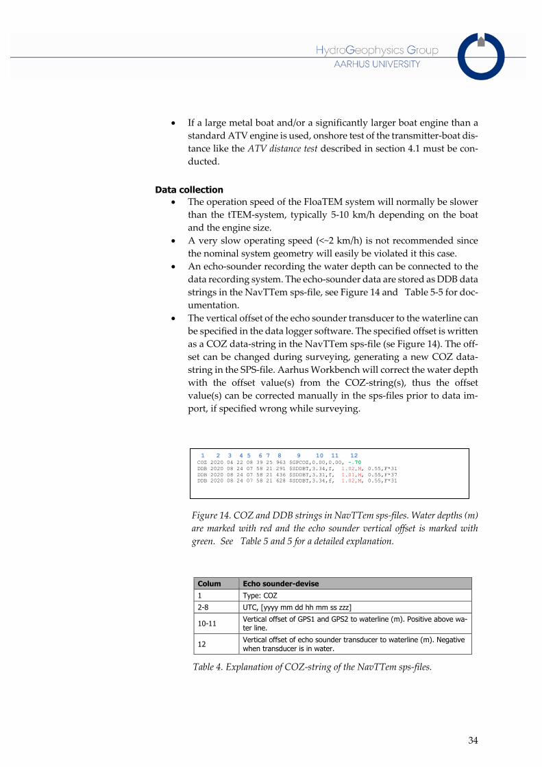
The vertical offset of the echo sounder transducer to the waterline can

be specified in the data logger software. The specified offset is written

as a COZ data-string in the NavTTem sps-file (se Figure 14). The off-

set can be changed during surveying, generating a new COZ data-

string in the SPS-file. Aarhus Workbench will correct the water depth

with the offset value(s) from the COZ-string(s), thus the offset

value(s) can be corrected manually in the sps-files prior to data im-

port, if specified wrong while surveying.

Colum Echo sounder-devise

1 Type: COZ


10-11 Vertical offset of GPS1 and GPS2 to waterline (m). Positive above wa-ter line.

12 Vertical offset of echo sounder transducer to waterline (m). Negative when transducer is in water.

Table 4. Explanation of COZ-string of the NavTTem sps-files.

1 2 3 4 5 6 7 8 9 10 11 12 COZ 2020 04 22 08 39 25 963 $GPCOZ,0.00,0.00, -.70

DDB 2020 08 24 07 58 21 291 $SDDBT,3.34,f, 1.02,M, 0.55,F*31

DDB 2020 08 24 07 58 21 436 $SDDBT,3.31,f, 1.01,M, 0.55,F*37

DDB 2020 08 24 07 58 21 628 $SDDBT,3.34,f, 1.02,M, 0.55,F*31

Figure 14. COZ and DDB strings in NavTTem sps-files. Water depths (m)

are marked with red and the echo sounder vertical offset is marked with

green. See Table 5 and 5 for a detailed explanation.

35

Colum Echo sounder-devise

1 Type: DDB


9 Standard $SDDBT string. https://www.eye4software.com/hydro-magic/documentation/nmea0183/ for detailed info.

12 Water depth in meters.

Table 5. Explanation of DDB-string of the NavTTem sps-files.

Data processing and inversion

Pre-processing of the echo-sounder data outside Aarhus Workbench

might be needed to filter out bad/false data points e.g. due to aquatic

plant vegetation.

The operation speed must be taken into account when setting up the

stacking of the data. The resulting sounding/model distance should

be approximately 10 m.

Water depth from the echo-sounder or from an external bathymetry

grid can be added as prior information on the depth to first layer in-

terface in the inversion setup.

If measured, the conductivity of the water column can also be in-

cluded as prior information in the inversion.

https://www.eye4software.com/hydromagic/documentation/nmea0183/

https://www.eye4software.com/hydromagic/documentation/nmea0183/

36

9 REFERENCES

tTEM-system Status for tTEM-kortlægninger, GFS-report, April 2019

Auken, E., N. Foged, J. Larsen, K. Lassen, P. Maurya, S. Dath, and T. Eiskjær, 2018, tTEM — A towed transient electromagnetic system for detailed 3D imaging of the top 70 m of the subsurface, GEOPHYSICS,E13-E22.

Auken, E., J. B. Pedersen, and P. K. Maurya, 2018, A new towed geophysical transient electromagnetic system for near-surface mapping, Preview, June 2018,33-35.

Behroozmand,A.A.,Auken,E., Knight,R., 2019, Assessment of Managed Aquifer Re-charge Sites Using a New Geophysical Imaging Method, Vadose Zone Journal, May 2019.

Kim, H., A. Høyer, R. Jakobsen, L. Thorling, J. Aamand, P. K. Maurya, A. V. Christian-sen, B. Hansen, 2019, 3D characterization of the subsurface redox architecture in com-plex geological settings, Science of the Total Environment 693 (2019).

Maurya, P.K., A. V. Christiansen, J. Pedersen, E. Auken, 2019, High resolution 3D sub-surface mapping using towed transient electromagnetic system - tTEM: case studies, Near Surface Geophysics.

TEM-test site calibration and validation Foged, N., E. Auken, A. V. Christiansen, and K. I. Sørensen, 2013, Test site calibration and validation of airborne and ground based TEM systems, Geophysics, 78, 2,E95-E106.

The tTEM System - System validation and comparison with PACES and ERT, December 2019, GFS-report.

FloaTEM John W. Lane, Martin A. Briggs, Pradip K. Maurya, Eric A. White, Jesper B. Pedersen, Esben Auken, Neil Terry, Burke Minsley, Wade Kress, Denis R. LeBlanc, Ryan Adams, Carole D. Johnson, Characterizing the diverse hydrogeology underlying rivers and es-tuaries using new floating transient electromagnetic methodology, Science of The Total Environment, Volume 740, 2020.

GERDA upload Reporting tTEM and SkyTEM data/models to GERDA using Aarhus Workbench, Febru-ary 2020, GFS-report.

APPENDIX 1 DOCUMENTATION OF THE GEX FILE

The geometry file contains all information about the tTEM system, e.g. calibration factors,

loop sizes, device positions, transmitter waveform, etc. used during the processing and in-

version of the data. The information from the geometry file is linked to the data during im-

port to in Aarhus Workbench.

For tTEM, only the full geometry file in gex-format is supported.

The format of the GEX –file is defined in an *.ini format and is explained in the example

below. The GEX-file is split up in a [General] block, a [Channel1] (LM), and Chan-

nel2] (HM) block and is keyword based. The order of the parameters/keywords within a

block does not matter.

The brown colored parameters in the GEX-file example are settings that can be looked up in

the RWB/SPS-files, while black colored parameters are values obtained by external measure-

ments, or other data/modeling settings.

/gex file for import of tTEM data to Aarhus Workbech

/Note: SI-units are used for all variables

/Text after a forward slash '/' are comments and are automatic skipped by the importer

/'[General]' or '[Channel#]' marks the start of the different sections in the gex file

[General]

Description=tTEM2_Offset

DataType= GroundTEM

/-------- Device positions ---------------------------------------------------------

GPSPosition1= 2.00 0.00 -1.20 /x,y,z (m) (z positive downward)

RxCoilPosition1= -9.28 0.00 -0.43

TxCoilPosition1= 0.00 0.00 -0.50

/-------- Low pass filter definition ------------------------------------------------

RxCoilLPFilter1= 0.7 450E+3 /Damping ratio Gaussian filter,Cut-off frequency

FrontGateDelay=1.9E-06 /Time (s) added to front gate time specified in the

/script, due to delay in the TX-RX commination

/---- Transmitter loop (Tx) definition -----------------------------------------------

LoopType=72 /Controls the source type. See remark below

NumberOfTurnsLM=1 /Number of Tx-loop turns, low moment

NumberOfTurnsHM=1 /Number of Tx-loop turns, high moment

TxLoopArea=8.00 /Area of Tx-loop (m2)

TxLoopPoint1= -02.00 -01.00 /Knee points x y (m) - clockwise order

TxLoopPoint2= 02.00 -01.00

TxLoopPoint3= 02.00 01.00

TxLoopPoint4= -02.00 01.00

Continues on next page…

Zero time definitions

In Aarhus Workbench (WB) and in the GEX-file all times are with zero time reference at the

begin of turn-off ramp (=transmitter turn off time).

In the RWB file the times in the section [MOMENTID_##] are related to zero time at trans-

mitter turn-on, while the SAMPLECENTERTIME are with zero reference at transmitter turn

off.

/---- Mics. --------------------------------------------------------------------------

GateNoForPowerLineMonitor=15 /Gate number to use for power line monitor

FreqForPowerLineMonitor=50.00 /Frequency for power line monitor

CalculateRawDataSTD=1 /1=Estimate uncertainty on raw stacks

/-------- Waveform definition ------------------------------------

/Low moment points Time (s) Normalized amplitude [0;1]

TXRampLM=

WaveformLMPoint01= -6.7400e-04 -0.000

WaveformLMPoint02= -6.6150e-04 -0.638

.

WaveformLMPoint38= 2.7000e-06 0.000

/High moment points Time (s) Normalized amplitude [0;1]

TXRampHM=

WaveformHMPoint01= -2.0370e-03 -0.000

WaveformHMPoint02= -2.0089e-03 -0.376

.

WaveformHMPoint40= 4.5000e-06 0.000

/------- Gate Time table (raw times)----------------------------------------

/Gate num Center Open Close (s)

GateTime01=2.190E-06 3.800E-07 4.000E-06

.

GateTime29=7.247E-04 6.434E-04 8.060E-04

GateTime30=9.092E-04 8.064E-04 1.012E-03

/-------- Low Moment, Z-coil channel -----------------------------

[Channel1]

RxCoilNumber=1 /Receiver coil number

GateTimeShift=-1.4E-06 /Time shift of gate times and frontgate time,(s)

GateFactor=1.05 /Factor shift of db/dt values (factor)

RemoveInitialGates=6 /Automatic disabling of time gate 1 to

RemoveInitial Gates in Aarhus Workbench

PrimaryFieldDampingFactor=1 /Primary field damping factor, used in the

modelig/iversion of the data

UniformDataSTD=0.03 /Relativ uniform STD for db/dt-data (all gates)

E.g. 0.03 = ~3%

NoGates=15 /Numbers of gates (from Gate Time table [1;NoGates])

RepFreq=1055 /Repetition frequency

FrontGateTime=2.0E-6 /Frontgate time (0=No front gate)

TiBLowPassFilter=1 6.79E+5 /LowPass filter in Transmitter instrument

TransmitterMoment=LM /Transmitter moment type (LM, HM, or Noise)

TxApproximateCurrent=5.2 /Approx. transmitter current. Must be within 25% of

the actual current

ReceiverPolarizationXYZ=Z /Receiver Polarization (X, Y, or Z)

/-------- High Moment, Z-coil channel ---------------

[Channel2]

RxCoilNumber=1 /Receiver coil number

GateTimeShift=-1.4E-06 /Time shift of gatetimeand font gate time, (s)

.

.

.

.

Documents

Guideline and standards for tTEM data collection