Please see the administrative notes on page iii

In accordance with the ISO/IEC Directives, Part 1, 2001, Clause A.5, this draft is submitted to the ISO national bodies for approval.

WARNING — THIS DOCUMENT IS NOT AN ISO GUIDE. IT IS DISTRIBUTED FOR REVIEW AND COMMENT. IT IS SUBJECT TO CHANGE WITHOUTNOTICE AND MAY NOT BE REFERRED TO AS A GUIDE.

RECIPIENTS OF THIS DRAFT ARE INVITED TO SUBMIT, WITH THEIR COMMENTS, NOTIFICATION OF ANY RELEVANT PATENT RIGHTS OF WHICH THEY ARE AWARE AND TO PROVIDE SUPPORTING DOCUMENTATION.

IN ADDITION TO THEIR EVALUATION AS BEING ACCEPTABLE FOR INDUSTRIAL, TECHNOLOGICAL, COMMERCIAL AND USER PURPOSES,DRAFT GUIDES MAY ON OCCASION HAVE TO BE CONSIDERED IN THE LIGHT OF THEIR POTENTIAL TO BECOME DOCUMENTS TO WHICH REFERENCE MAY BE MADE IN NATIONAL REGULATIONS.

© International Organization for Standardization, 2004

ISO GUM Suppl. 1 (DGUIDE 99998)

TMB

Voting begins on Voting terminates on 2004-05-14 2004-09-14

INTERNATIONAL ORGANIZATION FOR STANDARDIZATION • МЕЖДУНАРОДНАЯ ОРГАНИЗАЦИЯ ПО СТАНДАРТИЗАЦИИ • ORGANISATION INTERNATIONALE DE NORMALISATION

Guide to the expression of uncertainty in measurement (GUM) — Supplement 1: Numerical methods for the propagation of distributions

Guide pour l'expression de l'incertitude de mesure (GUM) — Supplément 1: Méthodes numériques pour la propagation de distribution

ICS 17.020

ISO GUM Suppl. 1 (IDGUIDE 99998)

PDF disclaimer This PDF file may contain embedded typefaces. In accordance with Adobe's licensing policy, this file may be printed or viewed but shall not be edited unless the typefaces which are embedded are licensed to and installed on the computer performing the editing. In downloading this file, parties accept therein the responsibility of not infringing Adobe's licensing policy. The ISO Central Secretariat accepts no liability in this area.

Adobe is a trademark of Adobe Systems Incorporated.

Details of the software products used to create this PDF file can be found in the General Info relative to the file; the PDF-creation parameters were optimized for printing. Every care has been taken to ensure that the file is suitable for use by ISO member bodies. In the unlikely event that a problem relating to it is found, please inform the Central Secretariat at the address given below.

Copyright notice

This ISO document is a Draft Guide and is copyright-protected by ISO. Except as permitted under the applicable laws of the user's country, neither this ISO draft nor any extract from it may be reproduced, stored in a retrieval system or transmitted in any form or by any means, electronic, photocopying, recording or otherwise, without prior written permission being secured.

Requests for permission to reproduce should be addressed to either ISO at the address below or ISO's member body in the country of the requester.

ISO copyright office Case postale 56 • CH-1211 Geneva 20 Tel. + 41 22 749 01 11 Fax + 41 22 749 09 47 E-mail copyright@iso.org Web www.iso.org

Reproduction may be subject to royalty payments or a licensing agreement.

Violators may be prosecuted.

ii © ISO 2004 – All rights reserved

ISO GUM Suppl. 1 (DGUIDE 99998)

© ISO 2004 — All rights reserved iii

For convenience in the management of the enquiry ballot, this draft is submitted under the reference ISO DGUIDE 99998. On publication the reference ISO DGUIDE 99998 will be discarded.

In accordance with the provisions of Council Resolution 15/1993 this document is circulated in the English language only.

Conformément aux dispositions de la Résolution du Conseil 15/1993, ce document est distribué en version anglaise seulement.

To expedite distribution, this document is circulated as received from the committee secretariat. ISO Central Secretariat work of editing and text composition will be undertaken at publication stage.

Pour accélérer la distribution, le présent document est distribué tel qu'il est parvenu du secrétariat du comité. Le travail de rédaction et de composition de texte sera effectué au Secrétariat central de l'ISO au stade de publication.

Supplement 1. 2004-03-16 : 2004

Guide to the Expression of Uncertainty in MeasurementSupplement 1Numerical Methods for the Propagation of Distributions

This version is intended for circulation to the mem-ber organizations of the JCGM and National Mea-surement Institutes for review.

Contents Page

Foreword . . . . . . . . . . . . . . . . . . . . . . . . . . . . . . 2

Introduction . . . . . . . . . . . . . . . . . . . . . . . . . . . 2

1 Scope . . . . . . . . . . . . . . . . . . . . . . . . . . . . . . 3

2 Notation and definitions . . . . . . . . . . . . . . 4

3 Concepts . . . . . . . . . . . . . . . . . . . . . . . . . . . 5

4 Assignment of probability density func-tions to the values of the input quantities . . 7

4.1 Probability density function assignmentfor some common circumstances . . . . . . . 7

4.2 Probability distributions from previousuncertainty calculations . . . . . . . . . . . . . 8

5 The propagation of distributions . . . . . . . 8

6 Calculation using Monte Carlo simulation 96.1 Rationale and overview . . . . . . . . . . . . . . 96.2 The number of Monte Carlo trials . . . . . . 126.3 Sampling from probability distributions . . 126.4 Evaluation of the model . . . . . . . . . . . . . 126.5 Distribution function for the output

quantity value . . . . . . . . . . . . . . . . . . . . 126.6 The estimate of the output quantity value

and the associated standard uncertainty . 136.7 Coverage interval for the output quantity

value . . . . . . . . . . . . . . . . . . . . . . . . . . . 146.8 Reporting the results . . . . . . . . . . . . . . . 146.9 Computation time . . . . . . . . . . . . . . . . . 156.10 Adaptive Monte Carlo procedure . . . . . . . 15

7 Validation of the law of propagation of un-certainty using Monte Carlo simulation . . . . 16

8 Examples . . . . . . . . . . . . . . . . . . . . . . . . . . . 178.1 Simple additive model . . . . . . . . . . . . . . 17

8.1.1 Normally distributed input quan-tities . . . . . . . . . . . . . . . . . . . . . . 17

8.1.2 Rectangularly distributed inputquantities with the same width . . 18

8.1.3 Rectangularly distributed inputquantities with different widths . . 19

8.2 Mass calibration . . . . . . . . . . . . . . . . . . . 208.2.1 Formulation . . . . . . . . . . . . . . . . . 208.2.2 Calculation . . . . . . . . . . . . . . . . . 20

8.3 Comparison loss in microwave power me-ter calibration . . . . . . . . . . . . . . . . . . . . 228.3.1 Formulation . . . . . . . . . . . . . . . . . 228.3.2 Calculation: uncorrelated input

quantities . . . . . . . . . . . . . . . . . . 228.3.3 Calculation: correlated input

quantities . . . . . . . . . . . . . . . . . . 25

Annexes

A Historical perspective . . . . . . . . . . . . . . . . 29

B Sensitivity coefficients . . . . . . . . . . . . . . . . 30

C Sampling from probability distributions . 31C.1 General distributions . . . . . . . . . . . . . . . 31C.2 Rectangular distribution . . . . . . . . . . . . . 31

C.2.1 Randomness tests . . . . . . . . . . . . 31C.2.2 A recommended rectangular ran-

dom number generator . . . . . . . . . 32C.3 Gaussian distribution . . . . . . . . . . . . . . . 32C.4 t–distribution . . . . . . . . . . . . . . . . . . . . . 32C.5 Multivariate Gaussian distribution . . . . . 33

D The comparison loss problem . . . . . . . . . . 35D.1 The analytic solution for a zero value of

the voltage reflection coefficient . . . . . . . . 35D.2 The law of propagation of uncertainty ap-

plied to the comparison loss problem . . . . 35D.2.1 Uncorrelated input quantities . . . . 35D.2.2 Correlated input quantities . . . . . 36

1

JCGM-WG1-SC1-N10

Supplement 1. 2004-03-16 : 2004

Foreword

This Supplement is concerned with the concept of thepropagation of distributions as a basis for the evaluationof uncertainty of measurement. This concept constitutesa generalization of the law of propagation of uncertaintygiven in the Guide to the Expression of Uncertainty inMeasurement (GUM) [3]. It thus facilitates the provi-sion of uncertainty evaluations that are more valid thanthose provided by the use of the law of propagation ofuncertainty in circumstances where the conditions forthe application of that law are not fulfilled. The prop-agation of distributions is consistent with the generalprinciples on which the GUM is based. An implemen-tation of the propagation of distributions is given thatuses Monte Carlo simulation.

In 1997 a Joint Committee for Guides in Metrology(JCGM), chaired by the Director of the BIPM, wascreated by the seven International Organizations thathad prepared the original versions of the GUM and theInternational Vocabulary of Basic and General Termsin Metrology (VIM). The Committee had the task ofthe ISO Technical Advisory Group 4 (TAG4), which haddeveloped the GUM and the VIM. The Joint Commit-tee, as was the TAG4, is formed by the BIPM withthe International Electrotechnical Commission (IEC),the International Federation of Clinical Chemistry andLaboratory Medicine (IFCC), the International Orga-nization for Standardization (ISO), the InternationalUnion of Pure and Applied Chemistry (IUPAC), theInternational Union of Pure and Applied Physics (IU-PAP) and the International Organization of LegalMetrology (OIML). A further organization joined theseseven international organizations, namely, the Interna-tional Laboratory Accreditation Cooperation (ILAC).Within JCGM two Working Groups have been estab-lished. Working Group 1, “Expression of Uncertaintyin Measurement”, has the task to promote the use ofthe GUM and to prepare supplements for its broad ap-plication. Working Group 2, “Working Group on In-ternational Vocabulary of Basic and General Terms inMetrology (VIM)”, has the task to revise and promotethe use of the VIM. The present Guide has been pre-pared by Working Group 1 of the JCGM.

Introduction

This Supplement is concerned with the concept ofthe propagation of probability distributions through amodel of measurement as a basis for the evaluation ofuncertainty of measurement, and its implementation byMonte Carlo simulation. The treatment applies to amodel having any number of input quantities, and a sin-gle (scalar-valued) output quantity (sometimes knownas the measurand). A second Supplement, in prepa-ration, is concerned with arbitrary numbers of outputquantities. In particular, the provision of the probabil-ity density function for the output quantity value per-mits the determination of a coverage interval for thatvalue corresponding to a prescribed coverage probabil-ity. The Monte Carlo simulation technique in generalprovides a practical solution for complicated models ormodels with input quantities having “large” uncertain-ties or asymmetric probability density functions. Theevaluation procedure based on probability distributionsis entirely consistent with the GUM, which states inSubclause 3.3.5 that “. . . a Type A standard uncertaintyis obtained from a probability density function derivedfrom an observed frequency distribution, while a Type Bstandard uncertainty is obtained from an assumed prob-ability density function based on the degree of beliefthat an event will occur . . . ”. It is also consistent inthe sense that it falls in the category of the “other an-alytical or numerical methods” [GUM Subclause G.1.5]permitted by the GUM. Indeed, the law of propagationof uncertainty can be derived from the propagation ofdistributions. Thus, the propagation of distributions isa generalization of the approach predominantly advo-cated in the GUM, in that it works with richer infor-mation than that conveyed by best estimates and theassociated standard uncertainties alone.

This supplement also provides a procedure for the vali-dation, in any particular case, of the use of the law ofpropagation of uncertainty.

This document is a supplement to the use of the GUMand is to be used in conjunction with it.

2

JCGM-WG1-SC1-N10

Supplement 1. 2004-03-16 : 2004

1 Scope

This Supplement provides guidance on the evaluation ofmeasurement uncertainty in situations where the con-ditions for the applicability of the law of propagationof uncertainty and related concepts are not fulfilled orit is unclear whether they are fulfilled. It can also beused in circumstances where there are difficulties in ap-plying the law of propagation of uncertainty, because ofthe complexity of the model, for example. This guidanceincludes a general alternative procedure, consistent withthe GUM, for the numerical evaluation of measurementuncertainty, suitable for implementation by computer.

In particular, this Supplement provides a procedure fordetermining a coverage interval for an output quantityvalue corresponding to a specified coverage probability.The intent is to determine this coverage interval to aprescribed degree of approximation. This degree of ap-proximation is relative to the realism of the model andthe quality of the information on which the probabil-ity density functions for the model input quantities arebased.

It is usually sufficient to report the measurement un-certainty to one or perhaps two significant decimal dig-its. Further digits would normally be spurious, becausethe information provided for the uncertainty evaluationis typically inaccurate, involving estimates and judge-ments. The calculation should be carried out in a wayto give a reasonable assurance that in terms of this in-formation these digits are correct. Guidance is given onthis aspect.

NOTE — This attitude compares with that in mathematicalphysics where a model (e.g., a partial differential equation) isconstructed and then solved numerically. The constructioninvolves idealizations and inexactly known values for geo-metric quantities and material constants, for instance. Thesolution process should involve the application of suitablenumerical methods in order to make supported statementsabout the quality of the solution obtained to the posed prob-lem.

This Supplement provides a general numerical pro-cedure, consistent with the broad principles ofthe GUM [GUM G.1.5], for carrying out the calcula-tions required as part of an evaluation of measurementuncertainty. The procedure applies to arbitrary mod-els having a single output quantity where the values ofthe input quantities are assigned any specified probabil-ity density functions, including asymmetric probabilitydensity functions [GUM G.5.3].

The approach operates with the probability densityfunctions for the values of the input quantities in or-der to determine the probability density function forthe output quantity value. This is the reason for the

description of the approach as the propagation of distri-butions. Unlike the GUM, it does not make use of thelaw of propagation of uncertainty. That approach oper-ates with the best estimates (expectations) of the val-ues of the input quantities and the associated standarduncertainties (and where appropriate the correspondingdegrees of freedom) in order to determine an estimate ofthe output quantity value, the associated standard un-certainty, and a coverage interval for the output quantityvalue. Whereas there are some limitations to that ap-proach, (a sound implementation of) the propagation ofdistributions will always provide a probability densityfunction for the output quantity value that is consistentwith the probability density functions for the values ofthe input quantities. Once the probability density func-tion for the output quantity value is available, its ex-pectation is taken as an estimate of the output quantityvalue, its standard deviation is used as the associatedstandard uncertainty, and a 95 % coverage interval forthe output quantity value is obtained from it.

NOTE — Some distributions, such as the Cauchy distribu-tion, which arise exceptionally, have no expectation or stan-dard deviation. A coverage interval can always be obtained,however.

The approach here obviates the need for “effective de-grees of freedom” [GUM G.6.4] in the determination ofthe expanded uncertainty, so avoiding the use of theWelch-Satterthwaite formula [GUM G.4.2] and hencethe approximation inherent in it.

The probability density function for the output quantityvalue is not in general symmetric. Consequently, a cov-erage interval for the output quantity value is not nec-essarily centred on the estimate of the output quantityvalue. There are many coverage intervals correspondingto a specified coverage probability. This Supplement canbe used to provide the shortest coverage interval.

NOTE — Sensitivity coefficients [GUM 5.1.3] are not aninherent part of the approach and hence the calculation orapproximation of the partial derivatives of the model withrespect to the input quantities is not required. Values akinto sensitivity coefficients can, however, be provided using avariant of the approach (Appendix B).

Typical of the uncertainty evaluation problems to whichthis Supplement can be applied include

— those where the contributory uncertainties maybe arbitrarily large, even comparable to the uncer-tainty associated with the estimate of the outputquantity value;

— those where the contributions to the uncertaintyassociated with the estimate of the output quan-tity value are not necessarily comparable in magni-

3

JCGM-WG1-SC1-N10

Supplement 1. 2004-03-16 : 2004

tude [GUM G.2.2];

— those where the probability distribution for theoutput quantity value is not Gaussian, since re-liance is not placed on the Central Limit Theo-rem [GUM G.2.1];

— those where the estimate of the output quan-tity value and the associated standard uncertainty arecomparable in magnitude, as for measurements at ornear the limit of detection;

— those in which the models have arbitrary degreesof non-linearity or complexity, since the determinationof the terms in a Taylor series approximation is notrequired [GUM 5.1.2];

— those in which asymmetric distributions for thevalues of the input quantities arise, e.g., when dealingwith the magnitudes of complex variables in acousti-cal, electrical and optical metrology;

— those in which it is difficult or inconvenient toprovide the partial derivatives of the model (or ap-proximations to these partial derivatives), as neededby the law of propagation of uncertainty (possiblywith higher-order terms) [GUM 8].

This Supplement can be used in cases of doubt to checkwhether the law of propagation of uncertainty is appli-cable. A validation procedure is provided for this pur-pose. Thus, the considerable investment in this use ofthe GUM is respected: the law of propagation of un-certainty procedure remains the main approach to thecalculation phase of uncertainty evaluation, certainly incircumstances where it is demonstrably applicable.

Guidance is given on the manner in which the propaga-tion of distributions can be carried out, without makingunquantified approximations.

This Supplement applies to mutually independent in-put quantities, where the value of each such quantityis assigned an appropriate probability density function,or mutually dependent input quantities, the values ofwhich have been assigned a joint probability densityfunction.

Models with more than one output quantity are thesubject of a further Supplement to the GUM that isin preparation.

2 Notation and definitions

For the purposes of this Supplement the definitions ofthe GUM [3], the International Vocabulary of Basic and

General Terms in Metrology (VIM) [4] and ISO 3534,Part 1 [20] apply.

JCGM-WG1 has decided that the subscript “c”[GUM 2.3.4, 5.1.1] for the combined standard uncer-tainty is redundant. The standard uncertainty associ-ated with an estimate y of an output quantity value Ycan therefore be written simply as u(y), but the useof uc(y) remains acceptable if it is helpful to empha-size the fact that it represents a combined standard un-certainty. Moreover, the qualifier “combined” in “com-bined standard uncertainty” is also regarded as super-fluous and may be omitted. One reason for the deci-sion is that the argument (here y) already indicates theestimate of the output quantity value with which thestandard uncertainty is associated. Another reason isthat frequently the results of one or more uncertaintyevaluations become the inputs to a subsequent uncer-tainty evaluation. The use of the subscript “c” and thequalifier “combined” are inappropriate in this regard.

This Supplement departs from the symbols often usedfor probability density function and distribution func-tion. The GUM uses the generic symbol f to refer to amodel and a probability density function. Little confu-sion arises in the GUM as a consequence of this usage.The situation in this Supplement is different. The con-cepts of model, probability density function and distri-bution function are central to following and implement-ing the procedure provided. Therefore, in place of thesymbols f and F to denote a probability density func-tion and a distribution function, the symbols g and G,respectively, are used. The symbol f is reserved for themodel.

Citations of the form [GUM 4.1.4] are to the indicated(sub)clauses of the GUM.

The decimal point is used as the symbol to separate theinteger part of a decimal number from its fractional part.A decimal comma is used for this purpose in continentalEurope.

In this Supplement the term law of propagation of un-certainty applies to the use of a first-order Taylor seriesapproximation to the model. The term is qualified ac-cordingly when a higher-order approximation is used.Sometimes the term is extended to apply also to the as-sumption of the applicability of the Central Limit The-orem as a basis for providing coverage intervals. Thecontext makes clear the usage in any particular case.

4

JCGM-WG1-SC1-N10

Supplement 1. 2004-03-16 : 2004

3 Concepts

A model of measurement having any number of inputquantities and a single (scalar-valued) output quantityis considered. For this case, the main stages in the de-termination of an estimate of the output quantity value,the associated standard uncertainty, and a coverage in-terval for the output quantity value are as follows.

a) Define the output quantity, the quantity requiredto be measured.

b) Decide the input quantities upon which the out-put quantity depends.

c) Develop a model relating the output quantity tothese input quantities.

d) On the basis of available knowledge assign proba-bility density functions [GUM C.2.5] —Gaussian (nor-mal), rectangular (uniform), etc.—to the values of theinput quantities.

NOTES

1 Assign instead a joint probability density function tothe values of those input quantities that are mutually de-pendent.

2 A probability density function for the values of morethan one input quantity is commonly called “joint” evenif the probability density functions for the values of all theinput quantities are mutually independent.

e) Propagate the probability density functions forthe values of the input quantities through the modelto obtain the probability density function for the out-put quantity value.

f) Obtain from the probability density function forthe output quantity value

1) its expectation, taken as the estimate of theoutput quantity value;

NOTE — The expectation may not be appropriate forall applications (Clause 6.1, [GUM 4.1.4]).

2) its standard deviation, taken as the standarduncertainty associated with the estimate of the out-put quantity value [GUM E.3.2];

3) an interval (the coverage interval) containingthe unknown output quantity value with a specifiedprobability (the coverage probability).

Stages a)–d) are regarded in this Supplement as for-mulation, and Stages e) and f) as calculation. Theformulation stages are carried out by the metrologist,

perhaps with expert support. (Advice on formulationstages a)–c) will be provided in a further Supplementto the GUM on modelling that is under development.)Guidance on the assignment of probability density func-tions (Stage d) above) is given in this Supplement forsome common cases. The calculation stages, e) and f),for which detailed guidance is provided here, require nofurther metrological information, and in principle canbe carried out to any required degree of approximation,relative to how well the formulation stages have beenundertaken.

A measurement model [GUM 4.1] is expressed by a func-tional relationship f :

Y = f(X), (1)

where Y is a single (scalar) output quantity (the out-put quantity) and X represents the N input quanti-ties (X1, . . . , XN )T.

NOTES

1 It is not necessary that Y is given explicitly in termsof X , i.e., f constitutes a formula. It is only neces-sary that a prescription is available for determining Ygiven X [GUM 4.1.2].

2 In this Supplement, T in the superscript position denotes“transpose”, and thus X represents X1, . . . , XN arranged asa column (vector) of values.

The GUM provides general guidance on many aspects ofthe above stages. It also contains a specific procedure,the law of propagation of uncertainty [GUM 5.1, 5.2],for the calculation phase of uncertainty evaluation.

The law of propagation of uncertainty has been adoptedby many organizations, is widely used and has been im-plemented in standards and guides on measurement un-certainty and also in computer packages. In order toapply this law, the values of the model input quantitiesare summarized by the expectations and standard devi-ations of the probability density functions for these val-ues. This information is “propagated” through a first-order Taylor series approximation to the model to pro-vide an estimate of the output quantity value and theassociated standard uncertainty. That estimate of theoutput quantity value is given by evaluating the modelat the best estimates of the values of the input quanti-ties. A coverage interval for the output quantity value isprovided based on taking the probability density func-tion for the output quantity value as Gaussian.

The intent of the GUM is to derive the expectation andstandard deviation of the probability density functionfor the output quantity value, having first determinedthe expectations and standard deviations of the proba-bility density functions for the values of the input quan-

5

JCGM-WG1-SC1-N10

Supplement 1. 2004-03-16 : 2004

tities.

NOTES

1 The best estimates of the values of the input quantitiesare taken as the expectations of the corresponding probabil-ity density functions [GUM 4.1.6].

2 The summaries of values of the input quantities also in-clude, where appropriate, the degrees of freedom of the stan-dard uncertainties associated with the estimates of the valuesof the input quantities [GUM 4.2.6].

3 The summaries of the values of the input quantities alsoinclude, where appropriate, covariances associated with theestimates of the values of input quantities [GUM 5.2.5].

4 The GUM [Note to GUM Subclause 5.1.2] states thatif the non-linearity of the model is significant, higher-orderterms in the Taylor series expansion must be included in theexpressions for the standard uncertainty associated with theestimate of the output quantity value.

5 If the analytic determination of the higher derivatives,required when the non-linearity of the model is significant,is difficult or error-prone, suitable software systems for au-tomatic differentiation can be used. Alternatively, thesederivatives can be calculated numerically using finite differ-ences [GUM 5.1.3]. Care should be taken, however, becauseof the effects of subtractive cancellation when forming dif-ferences in values of the model for close values of the inputquantities.

6 The most important terms of next highest order to beadded to those of the formula in GUM Subclause 5.1.2 for thestandard uncertainty are given in the Note to this subclause.Although not stated in the GUM, this formula applies whenthe values of Xi are Gaussian. In general, it would not applyfor other probability density functions.

7 The statement in the GUM [Note to GUM Sub-clause 5.1.2] concerning significant model non-linearity re-lates to input quantities that are mutually independent. Noguidance is given in the GUM if they are mutually depen-dent, but it is taken that the same statement would apply.

8 A probability density function related to a t–distributionis used instead of a Gaussian probability density function ifthe effective degrees of freedom associated with the estimateof the standard deviation of the probability density functionfor the output quantity value is finite [GUM G].

The calculation stages (Stages e) and f) above) ofthe GUM that use the law of propagation of uncertaintyand the abovementioned concepts can be summarized asthe following computational steps. Also see Figure 1.

a) Obtain from the probability density functions forthe values of the input quantities X1, . . . , XN , respec-tively, the expectation x = (x1, . . . , xN )T and thestandard deviations (standard uncertainties) u(x) =(u(x1), . . . , u(xN ))T. Use the joint probability den-sity function for the value of X instead if the Xi aremutually dependent.

NOTE — The Xi are regarded as random variables withpossible values ξi and expectations xi.

b) Take the covariances (mutual uncertain-ties) [GUM C] u(xi, xj) as Cov(Xi, Xj), thecovariances of mutually dependent pairs (Xi, Xj) ofinput quantities.

c) Form the partial derivatives of first order of fwith respect to the input quantities.

d) Calculate the estimate y of the output quantityvalue by evaluating the model at x.

e) Calculate the model sensitivity coefficients[GUM 5.1] as the above partial derivatives evaluatedat x.

f) Determine the standard uncertainty u(y) by com-bining u(x), the u(xi, xj) and the model sensitivitycoefficients [GUM Formulae (10) and (13)].

g) Calculate ν, the effective degrees of freedom of y,using the Welch-Satterthwaite formula [GUM For-mula (G.2b)].

h) Compute the expanded uncertainty Up, andhence a coverage interval for the output quantityvalue (having a stipulated coverage probability p),by forming the appropriate multiple of u(y) throughtaking the probability distribution of (y − Y )/u(y)as a standard Gaussian distribution (ν = ∞) or t–distribution (ν < ∞).

x1, u(x1) �

x2, u(x2) �

x3, u(x3) �

Y = f(X) � y, u(y)

Figure 1 — Illustration of the law of propagation of

uncertainty. The model has mutually independent

input quantities X = (X1, X2, X3)T, whose values are

estimated by xi with associated standard uncertain-

ties u(xi), for i = 1, 2, 3. The value of the output

quantity Y is estimated by y, with associated stan-

dard uncertainty u(y).

The computational steps above require the followingconditions to hold:

a) the non-linearity of f to be insignificant [Note toGUM 5.1.2];

6

JCGM-WG1-SC1-N10

Supplement 1. 2004-03-16 : 2004

b) the Central Limit Theorem [GUM G.2.1, G.6.6]to apply, implying the representativeness of the prob-ability density function for the output quantity valueby a Gaussian distribution or in terms of a t–distribution;

c) the adequacy of the Welch-Satterthwaite for-mula for calculating the effective degrees of free-dom [GUM G.4.2].

NOTE — The last two conditions are required for com-putational steps g) and h) above.

When these three conditions hold, the results from thesound application of the law of propagation of uncer-tainty are valid. These conditions apply in many cir-cumstances. The approach is not always applicable,however. This Supplement provides a more general ap-proach that does not require these conditions to hold.

4 Assignment of probability densityfunctions to the values of the inputquantities

In the first phase—formulation—of uncertainty eval-uation, the probability density functions for the val-ues of the input quantities of the model are as-signed [GUM 2.3.2, 3.3.5] based on an analysis of seriesof observations or based on scientific judgement [GUM2.3.3, 3.3.5] using all the relevant information [38], suchas historical data, calibrations and expert judgement.

The probability density function for the possible val-ues ξi of the ith input quantity Xi is denoted by gi(ξi)and that for the possible values of the output quantityvalue Y by g(η). The distribution function for Xi isdenoted by Gi(ξi) and that for Y by G(η). The prob-ability density functions and the distribution functionsare related by gi(ξi) = G′

i(ξi) and g(η) = G′(η).

When the input quantities are mutually dependent,in place of the N individual probability density func-tions gi(ξi), i = 1, . . . , N , there is a joint probabilitydensity function g(ξ). See Notes 1 and 2 at the end ofSection 5. Intermediate to these extremes, groups of theinput quantities may have values with joint probabilitydensity functions.

Clauses 4.2 and 4.3 of the GUM contain much relevantinformation on the assignment of probability densityfunctions.

NOTES

1 The Principle of Maximum Information Entropy can beapplied to assist in the assignment [7, 39, 40].

2 It may be possible to remove some mutual dependenciesby re-expressing some or all of the input quantities in termsof more fundamental mutually independent input quantitieson which the original input quantities depend [GUM F1.2.4,GUM H.1]. Such changes can simplify both the applicationof the law of propagation of uncertainty and the propagationof distributions. Details and examples are available [13].

4.1 Probability density function assign-ment for some common circumstances

Assignments of probability density functions to the in-put quantities are given in Table 1 for some commoncircumstances.

All available informationconcerning quantity X

Probability density function(PDF) assigned to the valueof X

The estimate x and theassociated standard uncer-tainty u(x)

The Gaussian PDFN(x, u2(x))

The estimate x (> 0), andX is known to be nonneg-ative

The exponential PDFwith expectation x, viz.,exp(−ξ/x)/x, for ξ ≥ 0, andzero otherwise.

Independent observationsof a quantity value takento follow a normal lawwith unknown expectationequal to the value of X.From a sample of size n,an arithmetic mean x anda standard deviation s havebeen calculated

Product of√

n/s and thet–distribution with argument(ξ − x)/(s/

√n) and n − 1 de-

grees of freedom and where xand s are known constants

The estimate x of the valueof a multivariate quan-tity X and the correspond-ing uncertainty matrix (co-variance matrix) V

The multivariate GaussianPDF N(x, V ) is assigned tothe value of X (Section 5,Note 2)

The endpoints a− and a+

of an interval containingthe value of X

The rectangular PDF withendpoints a− and a+

The lower and upper lim-its a− and a+ of an inter-val within which the valueof X is known to cycle si-nusoidally

The scaled and shifted arcsinePDF with endpoints a− anda+, viz., (2/π)/{(a+ − a−)2 −(2ξ − a+ − a−)2}1/2, for a− <ξ < a+, and zero otherwise[14], [17, Section 3.5]

Table 1 — The assignment of a probability density

function to the value of an input quantity X based

on available information for some common circum-

stances.

7

JCGM-WG1-SC1-N10

Supplement 1. 2004-03-16 : 2004

4.2 Probability distributions from previousuncertainty calculations

A previous uncertainty calculation may have provided aprobability distribution for the value of an output quan-tity that is to become an input quantity for a further un-certainty calculation. This probability distribution maybe available analytically in a recognized form, e.g., asa Gaussian probability density function, with values forits expectation and standard deviation. It may be avail-able as an approximation to the distribution function fora quantity value obtained from a previous application ofMonte Carlo simulation, for example. A means for de-scribing such a distribution function for a quantity valueis given in Clause 6.5.

5 The propagation of distributions

Several approaches can be used for the second phase —calculation — of uncertainty evaluation:

a) analytical methods;

b) uncertainty propagation based on replacing themodel by a first-order Taylor series approxima-tion [GUM 5.1.2] — the law of propagation of un-certainty;

c) as b), except that contributions derived fromhigher-order terms in the Taylor series approximationare included [Note to GUM 5.1.2];

d) numerical methods [GUM G.1.5] that implementthe propagation of distributions, specifically MonteCarlo simulation (Section 6).

NOTE — Analytical methods are ideal in that they do notintroduce any approximation. They are applicable in simplecases only, however. A treatment and examples are avail-able [7, 12]. These methods are not considered further inthis Supplement, apart from in the examples section (Sec-tion 8.1.1) for comparison purposes.

Techniques other than the law of propagation of uncer-tainty are permitted by the GUM [GUM G.1.5]. Theapproach advocated in this Supplement, based on thepropagation of distributions, is general. For linear orlinearized models and input quantities with values forwhich the probability density functions are Gaussian,the approach yields results consistent with the law ofpropagation of uncertainty. But in cases where the lawof propagation of uncertainty cannot be applied the ad-vocated approach still gives correct uncertainty state-ments.

In terms of the calculations required, there are threeclasses of uncertainty evaluation problem:

a) those for which a general approach is needed;

b) those for which uncertainty propagation based ona first-order Taylor series approximation is applicable;

c) those for which it is unclear which approachshould be followed.

For Class a), this Supplement provides a generic, broadlyapplicable approach based on the propagation of distri-butions. With respect to Class b), this Supplement doesnot provide new material. For Class c), this Supplementprovides a procedure for validating in any particular cir-cumstance the use of the law of propagation of uncer-tainty (possibly based on a higher-order Taylor seriesapproximation).

The propagation of the probability density func-tions gi(ξi), i = 1, . . . , N , for the values of the inputquantities through the model to provide the probabilitydensity function g(η) for the output quantity value isillustrated in Figure 2 for the case N = 3. This figureis the counterpart of Figure 1 for the law of propaga-tion of uncertainty. Like the GUM, this Supplement isconcerned with models having a single output quantity.

�

g3(ξ3)

�

g2(ξ2)

�g1(ξ1)

Y = f(X) �

g(η)

Figure 2 — Illustration of the propagation

of distributions. The model input quantities

are X = (X1, X2, X3)T. The probability density func-

tions gi(ξi), for Xi, i = 1, 2, 3, are Gaussian, triangular

and Gaussian, respectively. The probability density

function g(η) for the value of the output quantity Y is

indicated as being asymmetric, as can arise for non-

linear models. (An asymmetric g(η) can also arise

when the probability density functions for the val-

ues of the input quantities are asymmetric.)

NOTES

1 The only joint probability density functions consideredin this Supplement are multivariate Gaussian.

2 A multivariate Gaussian probability density functionwith expectation x = (x1, . . . , xN )T and uncertainty ma-trix V is given by

g(ξ) =1

((2π)N det V )1/2exp

{−1

2(ξ − x)TV −1(ξ − x)

}.

8

JCGM-WG1-SC1-N10

Supplement 1. 2004-03-16 : 2004

This probability density function reduces to the product of Nunivariate Gaussian probability density functions when thereare no covariance effects, for the following reason. In thatcase

V = diag(u2(x1), . . . , u2(xN )),

whence

g(ξ) =1

(2π)N/2u(x1) · · ·u(xN )exp

{−1

2

N∑i=1

(ξi − xi)2

u2(xi)

}

=

N∏i=1

gi(ξi),

with

gi(ξi) =1√

2πu(xi)exp

{− (ξi − xi)

2

2u2(xi)

}.

6 Calculation using Monte Carlo simu-lation

6.1 Rationale and overview

Monte Carlo simulation provides a general approachto numerically approximating the distribution func-tion G(η) for the value of the output quantity Y =f(X). The following GUM Subclause is relevant to theconcept embodied in Monte Carlo simulation:

An estimate of the measurand Y , denoted by y,is obtained from equation (1) [identical to ex-pression (1) of this Supplement] using input esti-mates x1, x2, . . . , xN for the values of the N quan-tities X1, X2, . . . , XN . Thus the output estimate y,which is the result of the measurement, is given by

y = f(x1, x2, . . . , xN ) . . . (2)

NOTE – In some cases the estimate y may be obtainedfrom

y = Y =1

n

n∑k=1

Yk =1

n

n∑k=1

f(X1,k, X2,k, . . . , XN,k)

That is, y is taken as the arithmetic mean or aver-

age (see 4.2.1) of n independent determinations Yk

of Y , each determination having the same uncertainty

and each being based on a complete set of observed

values of the N input quantities Xi obtained at the

same time. This way of averaging, rather than y =

f(X1, X2, . . . , XN ), where Xi = (∑n

k=1Xi,k)/n is the

arithmetic mean of the individual observations Xi,k,

may be preferable when f is a nonlinear function of

the input quantities X1, X2, . . . , XN , but the two ap-

proaches are identical if f is a linear function of the Xi

(see H.2 and H.4). [GUM 4.1.4]

Although the GUM formula (2) need not provide themost meaningful estimate of the output quantity value,

as stated in the note to GUM Subclause 4.1.4, repeatedabove, it plays a relevant role within Monte Carlo sim-ulation as an implementation of the propagation of dis-tributions.

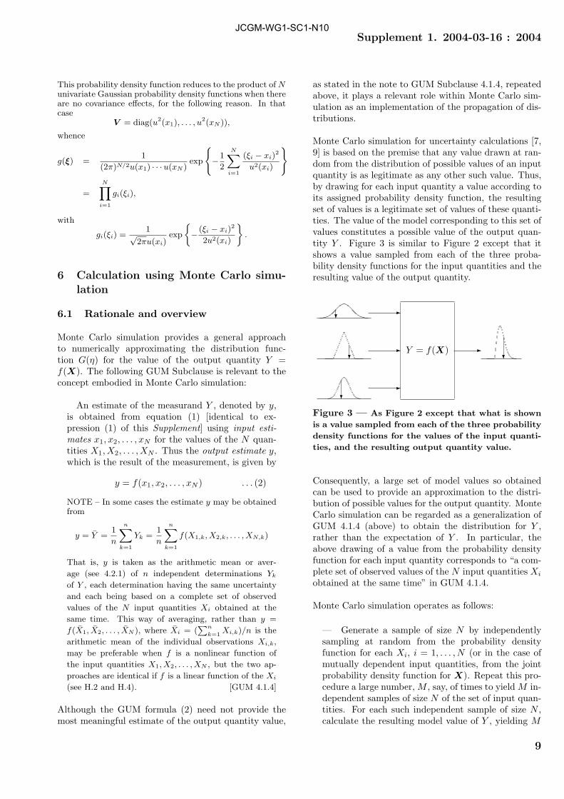
Monte Carlo simulation for uncertainty calculations [7,9] is based on the premise that any value drawn at ran-dom from the distribution of possible values of an inputquantity is as legitimate as any other such value. Thus,by drawing for each input quantity a value according toits assigned probability density function, the resultingset of values is a legitimate set of values of these quanti-ties. The value of the model corresponding to this set ofvalues constitutes a possible value of the output quan-tity Y . Figure 3 is similar to Figure 2 except that itshows a value sampled from each of the three proba-bility density functions for the input quantities and theresulting value of the output quantity.

��

��

��

Y = f(X) ��

Figure 3 — As Figure 2 except that what is shown

is a value sampled from each of the three probability

density functions for the values of the input quanti-

ties, and the resulting output quantity value.

Consequently, a large set of model values so obtainedcan be used to provide an approximation to the distri-bution of possible values for the output quantity. MonteCarlo simulation can be regarded as a generalization ofGUM 4.1.4 (above) to obtain the distribution for Y ,rather than the expectation of Y . In particular, theabove drawing of a value from the probability densityfunction for each input quantity corresponds to “a com-plete set of observed values of the N input quantities Xi

obtained at the same time” in GUM 4.1.4.

Monte Carlo simulation operates as follows:

— Generate a sample of size N by independentlysampling at random from the probability densityfunction for each Xi, i = 1, . . . , N (or in the case ofmutually dependent input quantities, from the jointprobability density function for X). Repeat this pro-cedure a large number, M , say, of times to yield M in-dependent samples of size N of the set of input quan-tities. For each such independent sample of size N ,calculate the resulting model value of Y , yielding M

9

JCGM-WG1-SC1-N10

Supplement 1. 2004-03-16 : 2004

values of Y in all.

NOTES

1 Appendix C provides information on sampling fromprobability distributions.

2 Clause 6.4 gives more explicit information concerningthe sample taken.

3 According to the Central Limit Theorem [30, p169],the arithmetic mean of the M values of the output quan-tity obtained in this manner converges as 1/M1/2 to theexpectation of the probability density function for thevalue of Y = f(X).

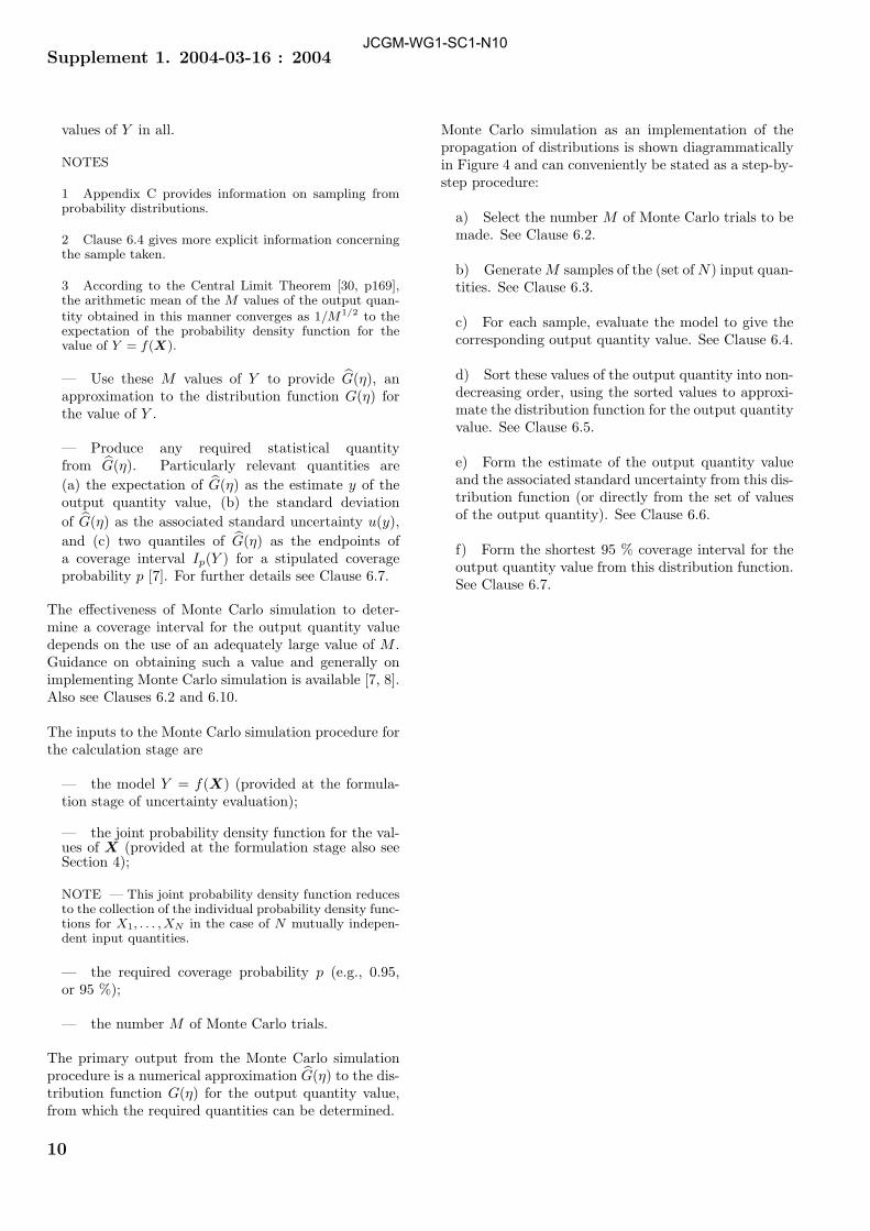
— Use these M values of Y to provide G(η), anapproximation to the distribution function G(η) forthe value of Y .

— Produce any required statistical quantityfrom G(η). Particularly relevant quantities are(a) the expectation of G(η) as the estimate y of theoutput quantity value, (b) the standard deviationof G(η) as the associated standard uncertainty u(y),and (c) two quantiles of G(η) as the endpoints ofa coverage interval Ip(Y ) for a stipulated coverageprobability p [7]. For further details see Clause 6.7.

The effectiveness of Monte Carlo simulation to deter-mine a coverage interval for the output quantity valuedepends on the use of an adequately large value of M .Guidance on obtaining such a value and generally onimplementing Monte Carlo simulation is available [7, 8].Also see Clauses 6.2 and 6.10.

The inputs to the Monte Carlo simulation procedure forthe calculation stage are

— the model Y = f(X) (provided at the formula-tion stage of uncertainty evaluation);

— the joint probability density function for the val-ues of X (provided at the formulation stage also seeSection 4);

NOTE — This joint probability density function reducesto the collection of the individual probability density func-tions for X1, . . . , XN in the case of N mutually indepen-dent input quantities.

— the required coverage probability p (e.g., 0.95,or 95 %);

— the number M of Monte Carlo trials.

The primary output from the Monte Carlo simulationprocedure is a numerical approximation G(η) to the dis-tribution function G(η) for the output quantity value,from which the required quantities can be determined.

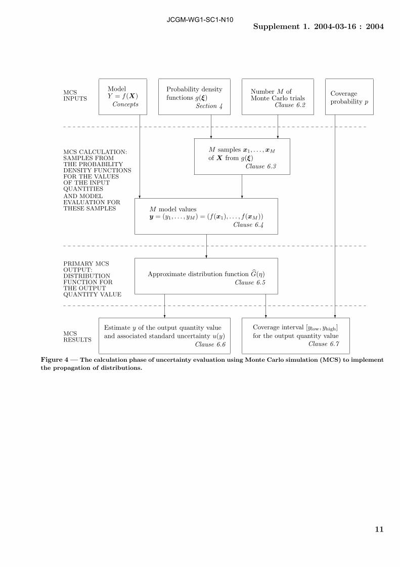
Monte Carlo simulation as an implementation of thepropagation of distributions is shown diagrammaticallyin Figure 4 and can conveniently be stated as a step-by-step procedure:

a) Select the number M of Monte Carlo trials to bemade. See Clause 6.2.

b) Generate M samples of the (set of N) input quan-tities. See Clause 6.3.

c) For each sample, evaluate the model to give thecorresponding output quantity value. See Clause 6.4.

d) Sort these values of the output quantity into non-decreasing order, using the sorted values to approxi-mate the distribution function for the output quantityvalue. See Clause 6.5.

e) Form the estimate of the output quantity valueand the associated standard uncertainty from this dis-tribution function (or directly from the set of valuesof the output quantity). See Clause 6.6.

f) Form the shortest 95 % coverage interval for theoutput quantity value from this distribution function.See Clause 6.7.

10

JCGM-WG1-SC1-N10

Supplement 1. 2004-03-16 : 2004

Coverage interval [ylow, yhigh]for the output quantity value

Clause 6.7

�

Estimate y of the output quantity valueand associated standard uncertainty u(y)

Clause 6.6

�

Approximate distribution function G(η)Clause 6.5

�

M model valuesy = (y1, . . . , yM ) = (f(x1), . . . , f(xM ))

Clause 6.4

�

M samples x1, . . . ,xM

of X from g(ξ)Clause 6.3

�

ModelY = f(X)Concepts

�

Probability densityfunctions g(ξ)

Section 4

�

Number M ofMonte Carlo trials

Clause 6.2

�

Coverageprobability p

MCSINPUTS

MCS CALCULATION:SAMPLES FROMTHE PROBABILITYDENSITY FUNCTIONSFOR THE VALUESOF THE INPUTQUANTITIESAND MODELEVALUATION FORTHESE SAMPLES

PRIMARY MCSOUTPUT:DISTRIBUTIONFUNCTION FORTHE OUTPUTQUANTITY VALUE

MCSRESULTS

Figure 4 — The calculation phase of uncertainty evaluation using Monte Carlo simulation (MCS) to implement

the propagation of distributions.

11

JCGM-WG1-SC1-N10

Supplement 1. 2004-03-16 : 2004

6.2 The number of Monte Carlo trials

A value of M , the number of Monte Carlo trials to bemade, needs to be selected. It can be chosen a priori,in which case there will be no direct control over thedegree of approximation delivered by the Monte Carloprocedure. The reason is that the number needed toprovide a prescribed degree of approximation will de-pend on the “shape” of the probability density functionfor the output quantity value and on the coverage prob-ability required. Also, the calculations are stochasticin nature, being based on random sampling. However,a value of M = 106 can often be expected to delivera 95 % coverage interval for the output quantity value,such that this length has a degree of approximation ofone or two significant decimal digits,.

Because there is no guarantee that this or any specificnumber will suffice, it is recommended to use a processthat selects M adaptively, i.e., as the trials progress.Some guidance in this regard is available [2, 7]. Alsosee Clause 6.10. A property of such a process is that ittakes a number of trials that is economically consistentwith the requirement to achieve the required degree ofapproximation [7].

NOTE — If the model is complicated, e.g., involving the so-lution of a finite-element model or a non-linear least-squaresproblem, because of the consequently prohibitive computingtime, it may not be possible to use a sufficiently large valueof M to obtain adequate distributional knowledge of the out-put quantity value. In such a case one approach could be asfollows. A relatively small value of M , 10 or 20, perhaps,would be used. The arithmetic mean and standard devi-ation of the resulting M values of Y would be taken as yand u(y), respectively, and a coverage interval for the out-put quantity value obtained by regarding Y to be distributedas y +Tu(y), where T denotes the t–distribution with M −1degrees of freedom.

6.3 Sampling from probability distribu-tions

In an implementation of the Monte Carlo procedure, Msamples xi, i = 1, . . . , M (Clause 6.2), are obtained fromthe probability density functions for the values of theinput quantities X. Samples would be obtained from ajoint (multivariate) Gaussian probability density func-tion when appropriate. Recommendations [8] concern-ing the manner in which this sampling can be carriedout are given in Appendix C for the commonest distri-butions, viz., the rectangular, Gaussian, t and multi-variate Gaussian. It is possible to sample from anyother distribution [7]. Some such distributions wouldbe those based on Monte Carlo results from a previousuncertainty calculation (Clauses 4.2 and 6.5).

NOTE — For the results of Monte Carlo simulation to

be statistically valid it is necessary that the pseudorandomnumber generators used to sample from the distributions re-quired have appropriate properties. Tests of randomness ofthe numbers produced by a generator are indicated in Ap-pendix C.

6.4 Evaluation of the model

The model is evaluated for each of the M samples fromeach of the probability density functions for the valuesof the N input quantities. Specifically, denote the Msamples by x1, . . . ,xM , where the rth sample xr con-tains values x1,r, . . . , xN,r, with xi,r a “draw” from theprobability density function for Xi. Then, the modelvalues are

yr = f(xr), r = 1, . . . , M.

NOTE — In Monte Carlo simulation the model is evalu-ated for each sample of the input quantities and hence forvalues that may be distanced by “several standard devia-tions” from the estimates of the values of the input quan-tities. For this reason some issues may arise regarding thenumerical procedure used to evaluate the model, e.g., ensur-ing its convergence (where iterative schemes are used) andnumerical stability. When applying the law of propagationof uncertainty, the model is evaluated only at the estimatesof the values of the input quantities or, if finite-differenceapproximations are used [GUM 5.1.3, Note 2], also at pointsperturbed by ± one standard deviation from the estimate ofthe value of each input quantity in turn. The user shouldensure that, where appropriate, the numerical methods usedto evaluate f are valid for a sufficiently large region centredon these estimates.

6.5 Distribution function for the outputquantity value

An approximation G(η) to the distribution func-tion G(η) for the output quantity value Y can be ob-tained as follows. Sort the values yr, r = 1, . . . , M ,of the output quantity provided by Monte Carlo simula-tion into non-decreasing order. Denote the sorted valuesby y(r), r = 1, . . . , M . Assign uniformly spaced cumu-lative probabilities pr = (r − 1/2)/M , r = 1, . . . , M , tothe ordered values [7].

NOTES

1 The term “non-decreasing” rather than “increasing” isused because of possible equalities among the values of yr.

2 A sorting algorithm taking a number of operations pro-portional to M log M should be be used [36]. A naive al-gorithm would take a time proportional to M2, making thecomputation time unnecessarily long. See Clause 6.9.

3 The values pr, r = 1, . . . , M , are the midpoints of Mcontiguous probability intervals of width 1/M between zeroand one.

12

JCGM-WG1-SC1-N10

Supplement 1. 2004-03-16 : 2004

Form G(η) as the piecewise-linear function joiningthe M points (y(r), pr), r = 1, . . . , M :

G(η) =r − 1/2

M+

η − y(r)

M(y(r+1) − y(r)),

y(r) ≤ η ≤ y(r+1), r = 1, . . . , M − 1. (2)

Figure 5 illustrates G(η) from a Monte Carlo simulationbased on M = 50 trials.

Figure 5 — The piecewise-linear function, form-

ing an approximation G(η) to the distribution func-

tion G(η), derived from 50 sampled values from a

Gaussian probability density function g(η) with ex-

pectation 10 and standard deviation 1.

NOTES

1 G(η) is defined only for values of η corresponding to val-ues of probability p in the interval 1/(2M) ≤ p ≤ 1−1/(2M).Indeed, it should not be used near the endpoints of this in-terval, e.g., for very large coverage probabilities in the caseof a symmetric or approximately symmetric distribution, be-cause it is less reliable there.

2 The values of y(r) (or yr), when assembled into a his-togram (with suitable cell widths) form a frequency distri-bution that, when normalized to have unit area, provides anapproximation g(η) to the probability density function g(η)for Y . Calculations are not generally carried out in terms ofthis histogram, the resolution of which depends on the choice

of cell size, but in terms of the approximation G(η) to thedistribution function G(η). The histogram can, however, beuseful as an aid to understanding the nature of the proba-bility density function, e.g., the extent of its asymmetry.

3 The very small value of M used to provide G(η) in Fig-ure 5 is for purposes of illustration only.

6.6 The estimate of the output quantityvalue and the associated standard un-certainty

The expectation y of the function G(η) (Expression (2))approximates the expectation of the probability density

function g(η) for the value of Y and is taken as the esti-mate y of the output quantity value. The standard devi-ation u(y) of G(η) approximates the standard deviationof g(η) and is taken as the standard uncertainty u(y)associated with y. y can be taken as the arithmeticmean

y =1M

M∑r=1

yr, (3)

formed from the M values y1, . . . , yM , and the standarddeviation u(y) determined from

u2(y) =1

M − 1

M∑r=1

(yr − y)2. (4)

NOTES

1 Formulae (3) and (4) do not in general provide valuesthat are identical to the expectation and standard deviation,

respectively, of G(η). The latter values are given by

y =1

M

M∑r=1

′′y(r) (5)

and

u2(y) =1

M

(M∑

r=1

′′(y(r) − y)2 − 1

6

M−1∑r=1

(y(r+1) − y(r))2

),

(6)

where the double prime on the summation in Expression (5)and on the first summation in Expression (6) indicates thatthe first and the last terms are to be taken with weight onehalf. For a sufficiently large value of M (104, say, or greater),the values obtained using Formulae (3) and (4) would gen-erally be indistinguishable for practical purposes from thosegiven by (5) and (6).

2 If the standard deviation is formed directly from the Mvalues y1, . . . , yM , it is important to use Formula (4) ratherthan the mathematically equivalent formula

u2(y) =M

M − 1

(1

M

M∑r=1

y2r − y2

).

For cases in which u(y) is much smaller than |y| (in whichcase the yr have a number of leading digits in common) thelatter formula suffers numerically from subtractive cancella-tion (involving a mean square less a squared mean). Thiseffect can be so severe that the resulting value may havetoo few correct significant decimal digits for the uncertaintyevaluation to be valid [6].

3 In some special circumstances, such as when one of theinput quantities has been assigned a probability density func-tion based on the t–distribution with fewer than three de-grees of freedom, and that input quantity has a dominant ef-fect, the expectation and the standard deviation of g(η) maynot exist. Formulae (5) and (6) (or Formulae (3) and (4))will not then provide meaningful results. A coverage intervalfor the output quantity value (Clause 6.7) can, however, beformed. See also the second Note in Section 1.

13

JCGM-WG1-SC1-N10

Supplement 1. 2004-03-16 : 2004

4 The value of y so obtained yields the smallest meansquared deviation over all possible estimates of the outputquantity value. However, the value will not in general agreewith the model evaluated at the estimates of the values ofthe input quantities [GUM 4.1.4]. When the model is linearin the input quantities, agreement (in a practical sense) willbe achieved for a large value of M . Whether this generallack of agreement is important depends on the application.The value of y, even in the limit as M → ∞, is not in gen-eral equal to the model evaluated at the expectations of theprobability density functions for the input quantities, unlessthe model is linear [GUM 4.1.4].

6.7 Coverage interval for the output quan-tity value

Let α denote any value between zero and 1− p, where pis the required coverage probability. The endpoints ofa 100p % coverage interval Ip(Y ) for the output quantityvalue are G−1(α) and G−1(p+α) i.e., the α– and (p+α)–quantiles of G(η). The β–quantile is the value of η suchthat G(η) = β. The choice α = 0.025 gives the coverageinterval defined by the 0.025– and 0.975–quantiles, pro-viding an I0.95(Y ) that is probabilistically symmetric.The probability is 2.5 % that the value of Y is smallerthan the left-hand endpoint of the interval and 2.5 %that it is larger than the right-hand endpoint. If g(η)is symmetric about its expectation, Ip(Y ) is symmet-ric about the estimate of the output quantity value y,and the left-hand and right-hand endpoints of Ip(Y ) areequidistant from y.

NOTE — For a symmetric probability density function forthe output quantity value Y , the procedure would, for asufficiently large value of M , give the same coverage intervalfor practical purposes as taking the product of the standarduncertainty and the coverage factor that is appropriate forthat probability density function. This probability densityfunction is generally not known analytically.

A value of α different from 0.025 would generally beappropriate were the probability density function asym-metric. Usually the shortest Ip(Y ) is required, becauseit corresponds to the best possible location of the valueof the output quantity Y within a specified probabil-ity. It is given by the value of α satisfying g(G−1(α)) =g(G−1(p + α)), if g(η) is single-peaked, and in generalby the value of α such that G−1(p + α) − G−1(α) is aminimum. If g(η) is symmetric, the shortest Ip(Y ) isgiven by taking α = (1 − p)/2.

The shortest Ip(Y ) can generally be obtained computa-tionally from G(η) by determining α such that G−1(p+α) − G−1(α) is a minimum.

Henceforth Ip(Y ) will denote the shortest 100p % cov-erage interval. The law of propagation of uncertainty,as in the GUM [3], provides the shortest such intervalfor the Gaussian (or scaled and shifted t–) distribution

assigned to the output quantity value. Therefore, it isappropriate in contrasting this approach with other ap-proaches to use the shortest 100p % coverage intervalfor the distributions they provide.

Figure 6 shows a distribution function G(η) for an asym-metric probability density function.

Figure 6 — A distribution function G(η) corre-

sponding to an asymmetric probability density func-

tion. Broken lines mark the endpoints of the prob-

abilistically symmetric 95 % coverage interval and

the corresponding probability points, viz., 0.025 and

0.975. Full lines mark the endpoints of the short-

est 95 % coverage interval and the corresponding

probability points, which are 0.006 and 0.956 in this

case. The lengths of the 95 % coverage intervals in

the two cases are 1.76 units and 1.69 units, respec-

tively.

6.8 Reporting the results

The estimate y of the output quantity value and the end-points ylow and yhigh of the coverage interval Ip(Y ) =[ylow, yhigh] corresponding to the coverage probabil-ity p for the output quantity value should be reportedto a number of decimal digits such that the leastsignificant digit is in the same position with respectto the decimal point as that for the standard uncer-tainty u(y) [GUM 7.2.6].

NOTES

1 One significant digit or two significant digits would beadequate to represent u(y) in many cases.

2 A factor influencing the choice of one or two significantdigits is the leading significant digit of u(y). If this digit is 1,the relative accuracy to which u(y) is reported is low if onedigit is used. If the leading significant digit is 9, the relativeaccuracy is almost an order of magnitude greater.

3 If the results are to be used within further calculations,

14

JCGM-WG1-SC1-N10

Supplement 1. 2004-03-16 : 2004

consideration should be given to whether additional digitsare required. There might be a repercussion for the numberof Monte Carlo trials (Clause 6.2).

As an example, suppose that it is meaningful to state

u(y) = 0.03 V.

Then, correspondingly, values of y and I0.95(Y ) mightbe

y = 1.02 V, I0.95(Y ) = [0.98, 1.09] V.

I0.95(Y ) is an asymmetric interval in this example. If itwere meaningful to report two significant digits in u(y),the values might be

y = 1.024 V, u(y) = 0.028 V,

I0.95(Y ) = [0.983, 1.088] V.

6.9 Computation time

The computation time for the Monte Carlo calculationsummarized in Clause 6.1 is dominated by that requiredfor the following three steps.

a) Take M samples from the probability densityfunction for the values of each of the input quanti-ties.

b) Make M corresponding evaluations of the model.

c) Sort the M resulting values into non-decreasingorder.

The time taken in Step a) is directly proportional to M .The same statement applies to Step b). The time takenin Step c) is proportional to M log M (if an efficient sortprocedure [36] is used).

If the model is very simple, the time in Step c) domi-nates, and the overall time taken is usually a few secondsfor M = 106 on a PC operating at several GHz. Oth-erwise, let T1 be the time in seconds taken to draw onesample from the probability density functions for theinput quantities and T2 that to make one evaluation ofthe model. Then, the overall time can be taken as es-sentially M×(T1+T2) s, or, if the model is complicated,as MT2 s.

The computation times taken on a personal computeroperating at several GHz are typically a few seconds forsimple models, seconds or perhaps a few minutes formore complicated models, and minutes or hours or evenlonger for very complicated models.

NOTE — An indication of the computation time requiredfor a Monte Carlo calculation can be obtained as follows.

Consider an artificial problem with a model consisting of thesum of five terms:

Y = cos X1 + sin X2 + tan−1 X3 + eX4 + X1/25 . (7)

Assign a Gaussian probability density function to each ofthe input quantities Xi. Make M = 106 Monte Carlo tri-als. Computation times observed for a 1 GHz Pentium 3 PCusing MATLAB [27]1) are summarized in Table 2. This infor-mation provides a simple basis for estimating the computa-tion time for other models, other values of M and other PCs.The times quoted apply to a particular PC, a particular im-plementation, and the version of MATLAB used, and aretherefore only indicative. They do not necessarily scale wellto other configurations.

Operation Time/sGenerate 5M random Gaussian numbers 1Form M model values 1Sort the M model values 3Total 5

Table 2 — Computation times for the main steps in

Monte Carlo simulation applied to the model (7),

where each Xi is assigned a Gaussian probability

density function and M = 106 Monte Carlo trials are

taken.

6.10 Adaptive Monte Carlo procedure

A basic implementation of an adaptive Monte Carlo pro-cedure can be described as follows. It is based on carry-ing out an increasing number of Monte Carlo trials untilthe various quantities of interest have stabilized in a sta-tistical sense. A quantity is deemed to have stabilizedif twice the standard deviation associated with the esti-mate of its value is less than the degree of approximationrequired in the standard uncertainty u(y).

NOTE — Typically, the more sensitive quantities are theendpoints of the coverage interval for the value of the out-put quantity Y . The expectation and the standard deviationas the estimate y of the output quantity value and the as-sociated standard uncertainty u(y), respectively, generally“converge” considerably faster.

A practical approach consists of carrying out a sequenceof Monte Carlo calculations, each containing a relativelysmall number, say, M = 104 trials. For each MonteCarlo calculation in the sequence, y, u(y) and I0.95(Y )are formed from the results obtained, as in Clauses 6.6and 6.7. Denote by y(h), u(y(h)), y

(h)low and y

(h)high the

values of y, u(y) and the left- and right-hand endpointsof I0.95(Y ) for the hth member of the sequence.

After the hth Monte Carlo calculation (apart fromthe first) in the sequence, the arithmetic mean y

1)Any identification of commercial products in this Supplementdoes not imply endorsement or that such products are best suitedfor the purpose.

15

JCGM-WG1-SC1-N10

Supplement 1. 2004-03-16 : 2004

of the values y(1), . . . , y(h) and the standard devi-ation sy associated with this arithmetic mean areformed. The counterparts of these statistics for y aredetermined for u(y), ylow and yhigh. If the largestof 2sy, 2su(y), 2sylow and 2syhigh does not exceed the de-gree of approximation required in u(y), the overall com-putation is regarded as having stabilized. The resultsfrom the total number of Monte Carlo trials taken arethen used to provide the estimate of the output quan-tity value, the associated standard uncertainty and thecoverage interval for the output quantity value.

7 Validation of the law of propagation ofuncertainty using Monte Carlo simu-lation

The law of propagation of uncertainty can be expectedto work well in many circumstances. However, it isgenerally difficult to quantify the effects of the approx-imations involved, viz., linearization [GUM 5.1.2], theWelch-Satterthwaite formula for the effective degreesof freedom [GUM G.4.2] and the assumption that theprobability distribution for the output quantity value isGaussian (i.e., that the Central Limit Theorem is appli-cable) [GUM G.2.1, G.6.6]. Indeed, the degree of diffi-culty of doing so would typically be considerably greaterthan that required to apply Monte Carlo simulation (as-suming suitable software were available [8]). Therefore,since these circumstances cannot readily be tested, anycases of doubt should be validated. To this end, sincethe propagation of distributions is more general, it isrecommended that both the law of propagation of un-certainty and Monte Carlo simulation be applied and theresults compared. Should the comparison be favourable,the law of propagation of uncertainty could be used onthis occasion and for sufficiently similar problems in thefuture. Otherwise, consideration could be given to usingMonte Carlo simulation instead.

Specifically, it is recommended that the two steps belowand the following comparison process be carried out.

a) Apply the law of propagation of uncertainty (pos-sibly based on a higher-order Taylor series approx-imation) [GUM 5] to yield a 95 % coverage inter-val y ± U0.95(y) for the output quantity value.

b) Apply Monte Carlo simulation (Section 6) to pro-vide values for the standard uncertainty u(y) and theendpoints ylow and yhigh of a 95 % coverage intervalfor the output quantity value.

NOTE — The process is described here in terms of a 95 %coverage interval, but other coverage intervals can be used.

A comparison procedure is based on the following objec-

tive: determine whether the coverage intervals obtainedby the law of propagation of uncertainty and MonteCarlo simulation agree to a stipulated degree of approx-imation. This degree of approximation is assessed interms of the endpoints of the coverage intervals andcorresponds to that given by expressing the standarduncertainty u(y) to what is regarded as a meaningfulnumber of significant decimal digits (cf. Clause 6.10).The procedure is as follows:

a) Let ndig denote the number of significant digitsregarded as meaningful in the numerical value of u(y).Usually, ndig = 1 or ndig = 2 (Clause 6.8). Expressthe value of u(y) in the form a × 10r, where a is anndig-digit integer and r an integer. The comparisonaccuracy is

δ =1210−r. (8)

EXAMPLES

1 — The estimate of the output quantity valuefor a nominally 100 g measurement standard ofmass [GUM 7.2.2] is y = 100.021 47 g. The stan-dard uncertainty u(y) = 0.000 35 g. Thus, ndig = 2and u(y) can be expressed as 35×10−5 g, and so a = 35and r = −5. Take δ = 1

2× 10−5 g = 0.000 005 g.

2 — As Example 1 except that only one significantdigit in u(y) is regarded as meaningful. Thus, ndig = 1and u(y) = 0.000 4 g = 4×10−4 g, giving a = 4 and r =−4. Thus, δ = 1

2× 10−4 g = 0.000 05 g.

3 — u(y) = 2 K. Then, ndig = 1 and u(y) = 2×100 K,giving a = 2 K and r = 0. Thus, δ = 1

2×100 K = 0.5 K.

b) Compare the coverage intervals obtained by thelaw of propagation of uncertainty and Monte Carlosimulation to determine whether the required num-ber of correct digits in the coverage interval providedby the law of propagation of uncertainty has been ob-tained. Specifically, determine the quantities

|y − U0.95(y) − ylow|, |y + U0.95(y) − yhigh|, (9)

viz., the absolute values of the differences of therespective endpoints of the two coverage intervals.Then, if both these quantities are no larger than δ,the comparison is successful and the law of propaga-tion of uncertainty has been validated in this instance.

NOTES

1 The validation applies for the specified coverage proba-bility only.

2 The choice of 95 % coverage interval will influence thecomparison. The shortest 95 % coverage interval should gen-erally be taken, for consistency with the shortest (probabilis-tically symmetric) coverage interval determined following theapplication of the law of propagation of uncertainty.

16

JCGM-WG1-SC1-N10

Supplement 1. 2004-03-16 : 2004

8 Examples

The examples given illustrate various aspects of thisSupplement. They show the application of the law ofpropagation of uncertainty with and without contribu-tions derived from higher-order terms in the Taylor se-ries approximation of the model function. They alsoshow the corresponding results provided by Monte Carlosimulation, and the use of the validation procedure ofSection 7. In some instances, solutions are obtained an-alytically for further comparison.

The first example (simple additive model) demonstratesthat the results from Monte Carlo simulation agree withthose from the application of the law of propagation ofuncertainty when the conditions hold for the latter toapply. The same model, but with changes to the prob-ability density functions assigned to the values of theinput quantities, is also considered to demonstrate somedepartures when the conditions do not hold. In the sec-ond example (mass calibration) the law of propagationof uncertainty is shown to be valid only if the contribu-tion derived from higher-order terms in the Taylor se-ries approximation of the model function are included.In the third example (electrical measurement), the lawof propagation of uncertainty is shown to yield invalidresults, even if all higher-order terms are taken into ac-count. Instances where the input quantities are uncor-related and correlated are treated.

NOTE — Although it is generally recommended that a fi-nal statement of the uncertainty be made to no more thanone or two significant decimal digits (Clause 6.8), more thantwo digits are reported in this section so as to highlight dif-ferences between the results obtained from the various ap-proaches.

8.1 Simple additive model

This example considers the simple additive model

Y = X1 + X2 + X3 + X4 (10)

for three different sets of probability density func-tions gi(ξi) assigned to the Xi. The Xi and Y areexpressed in (common) arbitrary units. For the firstset each gi(ξi) is a standard Gaussian probability den-sity function (expectation zero and standard deviationunity). For the second set each gi(ξi) is a rectangularprobability density function with zero expectation andunit standard deviation. The third set consists of threeidentical rectangular probability density functions anda fourth rectangular probability density function with astandard deviation ten times as large.

Further information concerning additive models suchas (10), where the probability density functions are

Gaussian or rectangular or a combination of both, isavailable [12].

8.1.1 Normally distributed input quantities

Assign a standard Gaussian probability density functionto the value of each Xi. The best estimates of the valuesof the input quantities are xi = 0, i = 1, 2, 3, 4, withassociated standard uncertainties u(xi) = 1.

The law of propagation of uncertainty [GUM 5] givesthe estimate y = 0.0 of the output quantity and theassociated standard uncertainty u(y) = 2.0, using a de-gree of approximation of two significant decimal digitsin u(y) (Clause 6.8). A 95 % coverage interval for thevalue of Y [GUM 6], based on a coverage factor of 1.96,is [−3.9, 3.9].

The application of the Monte Carlo procedure (Sec-tion 6) with M = 105 trials gives y = 0.0, u(y) = 2.0 andthe coverage interval [−3.9, 3.9]. Repetition with M =106 trials confirms these results to the number of deci-mal digits reported. The latter case was re-run (differ-ent random samplings being made from the probabilitydensity functions) to show the variability in the resultsobtained.

The results are summarized in the first four columnsof Table 3. Figure 7 shows some of the correspond-ing approximations obtained to the probability densityfunction for the output quantity value. For this exam-ple, such agreement would be expected for a sufficientlylarge value of M , because all the conditions hold for theapplicability of the law of propagation of uncertainty.

Method y u(y) 95 % CI dlow, dhigh VLPU 0.00 2.00 [-3.92, 3.92]MCS1 0.01 2.00 [-3.90, 3.92] 0.02, 0.00 YesMCS2 0.00 2.00 [-3.91, 3.94] 0.01, 0.02 YesMCS2 0.00 2.00 [-3.93, 3.91] 0.01, 0.01 Yes

Table 3 — The application to the model (10), with

each Xi assigned a standard Gaussian probability

density function (arbitrary units), of (a) the law of

propagation of uncertainty (LPU) and (b) Monte

Carlo simulation (MCS). MCS1 and MCS2 de-

note MCS with 105 and 106 trials, respectively, y

denotes the estimate of the value of the output

quantity Y , u(y) the standard uncertainty associated

with y, 95 % CI the 95 % coverage interval for the

output quantity value, dlow and dhigh the magnitudes

of the endpoint differences (9), and V whether the

results were validated to two significant digits.

Table 3 also shows the results of applying the com-parison procedure of Section 7. Using the terminologyof that section, ndig = 2, since two significant digits

17

JCGM-WG1-SC1-N10

Supplement 1. 2004-03-16 : 2004

Figure 7 — Approximations for the model (10),

with each Xi assigned a standard Gaussian prob-

ability density function, to the probability density

function for the output quantity value provided

by (a) the law of propagation of uncertainty and

(b) Monte Carlo simulation. For (b) the approxima-

tion constitutes a scaled frequency distribution (his-

togram) of the M = 106 values of Y . The endpoints of

the 95 % coverage interval provided by both meth-

ods are shown as vertical lines. The approximations

to the probability density function are visually indis-

tinguishable, as are those of the coverage intervals.

in u(y) are sought. Hence, u(y) = 2.0 = 20 × 10−1, andso a = 20 and r = −1. Thus the comparison accuracyis

δ =12× 10−1 = 0.05.

The magnitudes of the endpoint differences (Expres-sions ( 9)), and whether the law of propagation of uncer-tainty has been validated, are shown in the right-mosttwo columns of Table 3.

Figure 8 shows the length of the 95 % coverage interval(Clause 6.7), as a function of the probability value at itsleft-hand endpoint, for the approximation to the distri-bution function provided by Monte Carlo simulation. Asexpected for a symmetric probability density function,the interval takes its shortest length when symmetricallydisposed with respect to the expectation.

In contrast, Figure 9 shows the comparable figure for theasymmetric probability density function given in Fig-ure 16 (Clause 8.3), relating to a model of comparisonloss in power meter calibration. The 95 % coverage in-terval does not take its shortest length when symmet-rically disposed with respect to the expectation in thiscase. Indeed, the shortest 95 % coverage interval is asfar-removed as possible from an equiprobabilistic cov-erage interval, the left and right tail probabilities be-

Figure 8 — The length of the 95 % coverage in-

terval, as a function of the probability value at its

left-hand endpoint, for the approximation to the dis-

tribution function obtained by applying Monte Carlo

simulation to the model (10), where each Xi is as-

signed a standard Gaussian probability density func-

tion.

ing 5 % and 0 %, respectively, as opposed to 2.5 %and 2.5 %. The length of the equiprobabilistic cover-age interval is 50 % greater than that of the shortestcoverage interval.

Figure 9 — As Figure 8 except for a model of

comparison loss in power meter calibration (Sub-

clause 8.3.3).

8.1.2 Rectangularly distributed input quanti-ties with the same width

Assign a rectangular probability density function havingan expectation of zero and a standard deviation of unity(cf. Subclause 8.1.1) to the value of each Xi. Again,the best estimates of the values of the input quantities

18

JCGM-WG1-SC1-N10

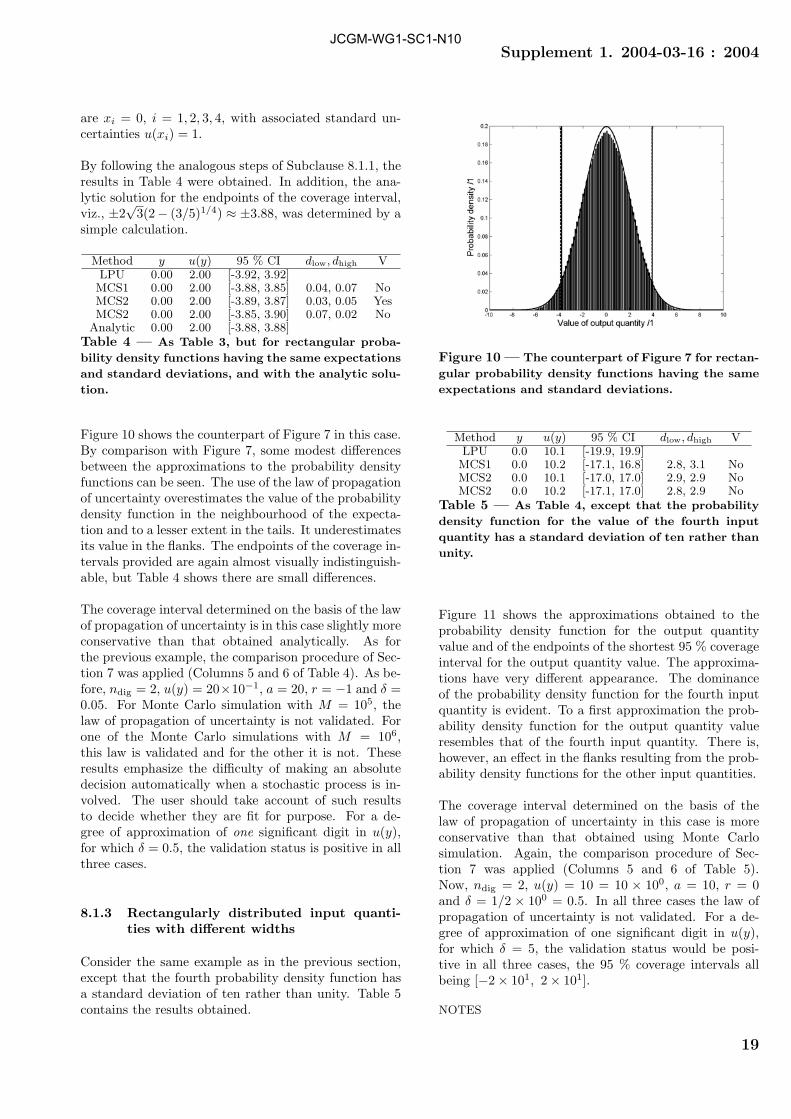
Supplement 1. 2004-03-16 : 2004

are xi = 0, i = 1, 2, 3, 4, with associated standard un-certainties u(xi) = 1.

By following the analogous steps of Subclause 8.1.1, theresults in Table 4 were obtained. In addition, the ana-lytic solution for the endpoints of the coverage interval,viz., ±2

√3(2− (3/5)1/4) ≈ ±3.88, was determined by a

simple calculation.

Method y u(y) 95 % CI dlow, dhigh VLPU 0.00 2.00 [-3.92, 3.92]MCS1 0.00 2.00 [-3.88, 3.85] 0.04, 0.07 NoMCS2 0.00 2.00 [-3.89, 3.87] 0.03, 0.05 YesMCS2 0.00 2.00 [-3.85, 3.90] 0.07, 0.02 No

Analytic 0.00 2.00 [-3.88, 3.88]Table 4 — As Table 3, but for rectangular proba-

bility density functions having the same expectations

and standard deviations, and with the analytic solu-

tion.

Figure 10 shows the counterpart of Figure 7 in this case.By comparison with Figure 7, some modest differencesbetween the approximations to the probability densityfunctions can be seen. The use of the law of propagationof uncertainty overestimates the value of the probabilitydensity function in the neighbourhood of the expecta-tion and to a lesser extent in the tails. It underestimatesits value in the flanks. The endpoints of the coverage in-tervals provided are again almost visually indistinguish-able, but Table 4 shows there are small differences.

The coverage interval determined on the basis of the lawof propagation of uncertainty is in this case slightly moreconservative than that obtained analytically. As forthe previous example, the comparison procedure of Sec-tion 7 was applied (Columns 5 and 6 of Table 4). As be-fore, ndig = 2, u(y) = 20×10−1, a = 20, r = −1 and δ =0.05. For Monte Carlo simulation with M = 105, thelaw of propagation of uncertainty is not validated. Forone of the Monte Carlo simulations with M = 106,this law is validated and for the other it is not. Theseresults emphasize the difficulty of making an absolutedecision automatically when a stochastic process is in-volved. The user should take account of such resultsto decide whether they are fit for purpose. For a de-gree of approximation of one significant digit in u(y),for which δ = 0.5, the validation status is positive in allthree cases.

8.1.3 Rectangularly distributed input quanti-ties with different widths

Consider the same example as in the previous section,except that the fourth probability density function hasa standard deviation of ten rather than unity. Table 5contains the results obtained.

Figure 10 — The counterpart of Figure 7 for rectan-

gular probability density functions having the same

expectations and standard deviations.

Method y u(y) 95 % CI dlow, dhigh VLPU 0.0 10.1 [-19.9, 19.9]MCS1 0.0 10.2 [-17.1, 16.8] 2.8, 3.1 NoMCS2 0.0 10.1 [-17.0, 17.0] 2.9, 2.9 NoMCS2 0.0 10.2 [-17.1, 17.0] 2.8, 2.9 No

Table 5 — As Table 4, except that the probability

density function for the value of the fourth input

quantity has a standard deviation of ten rather than

unity.

Figure 11 shows the approximations obtained to theprobability density function for the output quantityvalue and of the endpoints of the shortest 95 % coverageinterval for the output quantity value. The approxima-tions have very different appearance. The dominanceof the probability density function for the fourth inputquantity is evident. To a first approximation the prob-ability density function for the output quantity valueresembles that of the fourth input quantity. There is,however, an effect in the flanks resulting from the prob-ability density functions for the other input quantities.

The coverage interval determined on the basis of thelaw of propagation of uncertainty in this case is moreconservative than that obtained using Monte Carlosimulation. Again, the comparison procedure of Sec-tion 7 was applied (Columns 5 and 6 of Table 5).Now, ndig = 2, u(y) = 10 = 10 × 100, a = 10, r = 0and δ = 1/2 × 100 = 0.5. In all three cases the law ofpropagation of uncertainty is not validated. For a de-gree of approximation of one significant digit in u(y),for which δ = 5, the validation status would be posi-tive in all three cases, the 95 % coverage intervals allbeing [−2 × 101, 2 × 101].

NOTES

19

JCGM-WG1-SC1-N10

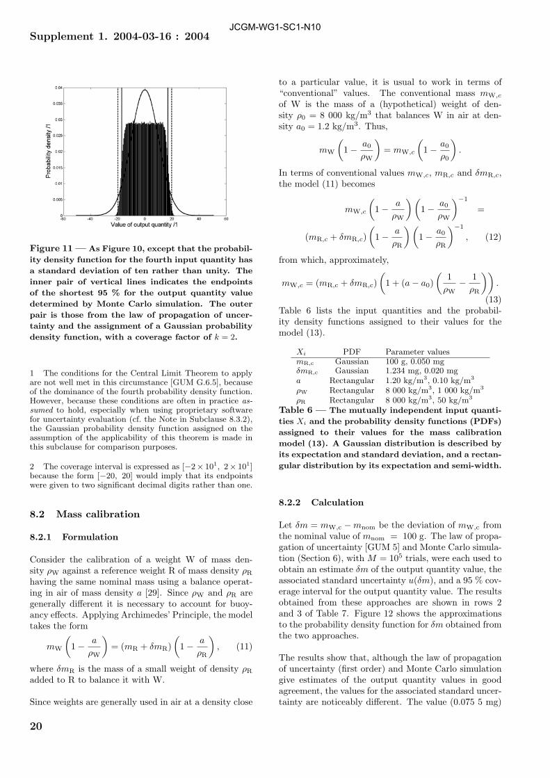
Supplement 1. 2004-03-16 : 2004

Figure 11 — As Figure 10, except that the probabil-

ity density function for the fourth input quantity has

a standard deviation of ten rather than unity. The

inner pair of vertical lines indicates the endpoints

of the shortest 95 % for the output quantity value

determined by Monte Carlo simulation. The outer

pair is those from the law of propagation of uncer-

tainty and the assignment of a Gaussian probability

density function, with a coverage factor of k = 2.

1 The conditions for the Central Limit Theorem to applyare not well met in this circumstance [GUM G.6.5], becauseof the dominance of the fourth probability density function.However, because these conditions are often in practice as-sumed to hold, especially when using proprietary softwarefor uncertainty evaluation (cf. the Note in Subclause 8.3.2),the Gaussian probability density function assigned on theassumption of the applicability of this theorem is made inthis subclause for comparison purposes.

2 The coverage interval is expressed as [−2× 101, 2× 101]because the form [−20, 20] would imply that its endpointswere given to two significant decimal digits rather than one.

8.2 Mass calibration

8.2.1 Formulation

Consider the calibration of a weight W of mass den-sity ρW against a reference weight R of mass density ρR

having the same nominal mass using a balance operat-ing in air of mass density a [29]. Since ρW and ρR aregenerally different it is necessary to account for buoy-ancy effects. Applying Archimedes’ Principle, the modeltakes the form

mW

(1 − a

ρW

)= (mR + δmR)

(1 − a

ρR

), (11)

where δmR is the mass of a small weight of density ρR

added to R to balance it with W.

Since weights are generally used in air at a density close

to a particular value, it is usual to work in terms of“conventional” values. The conventional mass mW,c

of W is the mass of a (hypothetical) weight of den-sity ρ0 = 8 000 kg/m3 that balances W in air at den-sity a0 = 1.2 kg/m3. Thus,

mW

(1 − a0

ρW

)= mW,c

(1 − a0

ρ0

).

In terms of conventional values mW,c, mR,c and δmR,c,the model (11) becomes

mW,c

(1 − a

ρW

) (1 − a0

ρW

)−1

=

(mR,c + δmR,c)(

1 − a

ρR

) (1 − a0

ρR

)−1

, (12)

from which, approximately,

mW,c = (mR,c + δmR,c)(

1 + (a − a0)(

1ρW

− 1ρR

)).

(13)Table 6 lists the input quantities and the probabil-ity density functions assigned to their values for themodel (13).

Xi PDF Parameter valuesmR,c Gaussian 100 g, 0.050 mgδmR,c Gaussian 1.234 mg, 0.020 mga Rectangular 1.20 kg/m3, 0.10 kg/m3

ρW Rectangular 8 000 kg/m3, 1 000 kg/m3

ρR Rectangular 8 000 kg/m3, 50 kg/m3

Table 6 — The mutually independent input quanti-

ties Xi and the probability density functions (PDFs)

assigned to their values for the mass calibration

model (13). A Gaussian distribution is described by

its expectation and standard deviation, and a rectan-

gular distribution by its expectation and semi-width.

8.2.2 Calculation

Let δm = mW,c − mnom be the deviation of mW,c fromthe nominal value of mnom = 100 g. The law of propa-gation of uncertainty [GUM 5] and Monte Carlo simula-tion (Section 6), with M = 105 trials, were each used toobtain an estimate δm of the output quantity value, theassociated standard uncertainty u(δm), and a 95 % cov-erage interval for the output quantity value. The resultsobtained from these approaches are shown in rows 2and 3 of Table 7. Figure 12 shows the approximationsto the probability density function for δm obtained fromthe two approaches.

The results show that, although the law of propagationof uncertainty (first order) and Monte Carlo simulationgive estimates of the output quantity values in goodagreement, the values for the associated standard uncer-tainty are noticeably different. The value (0.075 5 mg)

20

JCGM-WG1-SC1-N10

Supplement 1. 2004-03-16 : 2004

Meth- δm, u(δm) 95 % CI dlow, dhigh Vod /mg /mg endpoints /mgLPU1 1.234 0, 0.053 9 1.128 4, 1.339 6 0.043 9, 0.044 6 NoMCS 1.234 3, 0.075 5 1.084 5, 1.384 2LPU2 1.234 0, 0.075 0 1.087 0, 1.381 0 0.002 5, 0.003 2 Yes

Table 7 — Results of the calculation phase for

the mass calibration model (13) from (a) the law

of propagation of uncertainty (LPU1), (b) Monte

Carlo simulation (MCS) with 105 trials, and (c) the

law of propagation of uncertainty with second order

terms (LPU2). δm denotes the estimate of the out-

put quantity value, u(δm) the standard uncertainty

associated with δm, 95 % CI endpoints the endpoints

of the 95 % coverage interval for the output quantity

value, dlow and dhigh the magnitudes of the endpoint

differences (9), and V whether the results were val-

idated to two significant digits.

of u(δm) returned by Monte Carlo simulation is 40 %larger than that (0.053 9 mg) returned by the law ofpropagation of uncertainty (first order). The latter (firstorder) is thus optimistic in this respect. There is goodagreement between the value of u(δm) determined byMonte Carlo simulation and that (0.075 0 mg) providedby the law of propagation of uncertainty with second-order terms.

Table 8 lists the partial derivatives of first order for themodel (13) with respect to the values of the input quan-tities together with the model sensitivity coefficients,viz., these derivatives evaluated at the estimates of thevalues of the input quantities. These derivatives indicatethat for the purposes of the law of propagation of un-certainty the model for this example can be consideredas being replaced by the simple additive model

mW,c = mR,c + δmR,c.

Monte Carlo simulation makes no such (implied) ap-proximation to the model.

Table 7 also shows in the right-most two columns theresults of applying the comparison procedure of Sec-tion 7 in the case where one significant digit in u(y) isregarded as meaningful. Using the terminology of thatsection, ndig = 1, since a degree of approximation of onesignificant digit in u(y) is required. Hence, u(δm) =0.08 = 8 × 10−2, and so a = 8 and r = −2. Thus δ =1/2×10−2 = 0.005. The magnitudes of the endpoint dif-ferences (Expressions (9)) are shown, and whether thelaw of propagation of uncertainty has been validated. Ifonly first-order terms are accounted for, the applicationof the law of propagation of uncertainty is not validated.If second-order terms are accounted for [GUM 5.1.2], thelaw of propagation of uncertainty is validated.

NOTES

Figure 12 — Approximations to the probability

density function for the output quantity value δm

obtained using the law of propagation of uncertainty

and Monte Carlo simulation. The solid curve rep-

resents a Gaussian probability density function with

parameters given by this law. The inner pair of ver-

tical lines defines a 95 % coverage interval for δm

returned by the law of propagation of uncertainty

based on this probability density function. The his-

togram is the scaled frequency distribution obtained

from the Monte Carlo simulation values as an ap-

proximation to the probability density function. The

outer pair of vertical lines define a 95 % coverage in-

terval for δm based on this approximation.

Xi Partial Sensitivityderivative coefficient

mR,c 1 + (a − a0)(

1ρW

− 1ρR

)1

δmR,c 1 + (a − a0)(

1ρW

− 1ρR

)1

a (mR,c + δmR,c)(

1ρW

− 1ρR

)0

ρW −(mR,c + δmR,c)(a − a0)(

1ρ2W

)0

ρR −(mR,c + δmR,c)(a − a0)(

1ρ2R

)0

Table 8 — Model sensitivity coefficients for the

mass calibration model (13).

1 Applying the law of propagation of uncertainty to the“exact” model (12) is made difficult by the algebraic com-plexity of the partial derivatives. Applying Monte Carlo sim-ulation is no more complicated, because only model valuesneed be evaluated.

2 Results obtained from applying the law of propagationof uncertainty and Monte Carlo simulation procedures usingthe “exact model” (12) indicate that the approximation (13)is very good.

21

JCGM-WG1-SC1-N10

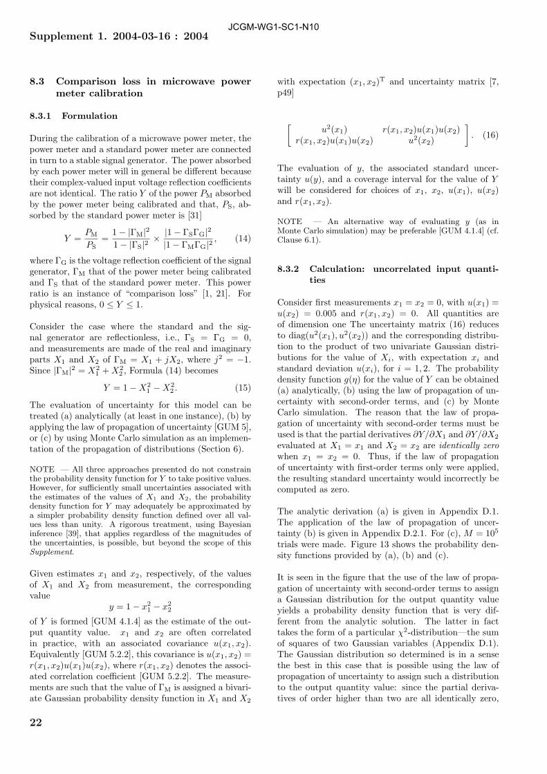
Supplement 1. 2004-03-16 : 2004

8.3 Comparison loss in microwave powermeter calibration

8.3.1 Formulation

During the calibration of a microwave power meter, thepower meter and a standard power meter are connectedin turn to a stable signal generator. The power absorbedby each power meter will in general be different becausetheir complex-valued input voltage reflection coefficientsare not identical. The ratio Y of the power PM absorbedby the power meter being calibrated and that, PS, ab-sorbed by the standard power meter is [31]

Y =PM

PS=

1 − |ΓM|21 − |ΓS|2 × |1 − ΓSΓG|2

|1 − ΓMΓG|2 , (14)

where ΓG is the voltage reflection coefficient of the signalgenerator, ΓM that of the power meter being calibratedand ΓS that of the standard power meter. This powerratio is an instance of “comparison loss” [1, 21]. Forphysical reasons, 0 ≤ Y ≤ 1.

Consider the case where the standard and the sig-nal generator are reflectionless, i.e., ΓS = ΓG = 0,and measurements are made of the real and imaginaryparts X1 and X2 of ΓM = X1 + jX2, where j2 = −1.Since |ΓM|2 = X2

1 + X22 , Formula (14) becomes

Y = 1 − X21 − X2

2 . (15)

The evaluation of uncertainty for this model can betreated (a) analytically (at least in one instance), (b) byapplying the law of propagation of uncertainty [GUM 5],or (c) by using Monte Carlo simulation as an implemen-tation of the propagation of distributions (Section 6).

NOTE — All three approaches presented do not constrainthe probability density function for Y to take positive values.However, for sufficiently small uncertainties associated withthe estimates of the values of X1 and X2, the probabilitydensity function for Y may adequately be approximated bya simpler probability density function defined over all val-ues less than unity. A rigorous treatment, using Bayesianinference [39], that applies regardless of the magnitudes ofthe uncertainties, is possible, but beyond the scope of thisSupplement.

Given estimates x1 and x2, respectively, of the valuesof X1 and X2 from measurement, the correspondingvalue

y = 1 − x21 − x2

2

of Y is formed [GUM 4.1.4] as the estimate of the out-put quantity value. x1 and x2 are often correlatedin practice, with an associated covariance u(x1, x2).Equivalently [GUM 5.2.2], this covariance is u(x1, x2) =r(x1, x2)u(x1)u(x2), where r(x1, x2) denotes the associ-ated correlation coefficient [GUM 5.2.2]. The measure-ments are such that the value of ΓM is assigned a bivari-ate Gaussian probability density function in X1 and X2

with expectation (x1, x2)T and uncertainty matrix [7,p49]

[u2(x1) r(x1, x2)u(x1)u(x2)

r(x1, x2)u(x1)u(x2) u2(x2)

]. (16)

The evaluation of y, the associated standard uncer-tainty u(y), and a coverage interval for the value of Ywill be considered for choices of x1, x2, u(x1), u(x2)and r(x1, x2).

NOTE — An alternative way of evaluating y (as inMonte Carlo simulation) may be preferable [GUM 4.1.4] (cf.Clause 6.1).

8.3.2 Calculation: uncorrelated input quanti-ties

Consider first measurements x1 = x2 = 0, with u(x1) =u(x2) = 0.005 and r(x1, x2) = 0. All quantities areof dimension one The uncertainty matrix (16) reducesto diag(u2(x1), u2(x2)) and the corresponding distribu-tion to the product of two univariate Gaussian distri-butions for the value of Xi, with expectation xi andstandard deviation u(xi), for i = 1, 2. The probabilitydensity function g(η) for the value of Y can be obtained(a) analytically, (b) using the law of propagation of un-certainty with second-order terms, and (c) by MonteCarlo simulation. The reason that the law of propa-gation of uncertainty with second-order terms must beused is that the partial derivatives ∂Y/∂X1 and ∂Y/∂X2

evaluated at X1 = x1 and X2 = x2 are identically zerowhen x1 = x2 = 0. Thus, if the law of propagationof uncertainty with first-order terms only were applied,the resulting standard uncertainty would incorrectly becomputed as zero.

The analytic derivation (a) is given in Appendix D.1.The application of the law of propagation of uncer-tainty (b) is given in Appendix D.2.1. For (c), M = 105

trials were made. Figure 13 shows the probability den-sity functions provided by (a), (b) and (c).

It is seen in the figure that the use of the law of propa-gation of uncertainty with second-order terms to assigna Gaussian distribution for the output quantity valueyields a probability density function that is very dif-ferent from the analytic solution. The latter in facttakes the form of a particular χ2-distribution—the sumof squares of two Gaussian variables (Appendix D.1).The Gaussian distribution so determined is in a sensethe best in this case that is possible using the law ofpropagation of uncertainty to assign such a distributionto the output quantity value: since the partial deriva-tives of order higher than two are all identically zero,

22

JCGM-WG1-SC1-N10

Supplement 1. 2004-03-16 : 2004

the solution obtained essentially corresponds to takingall Taylor-series terms into account, i.e., the “full non-linearity” of the problem. It can therefore be concludedthat the reason for the departure from the analytical so-lution of the results of the use of the approach based onthe law of propagation of uncertainty is that a Gaussianprobability density function is assigned to the outputquantity value. Evidently, no Gaussian probability den-sity function, however it is obtained, could adequatelyrepresent the analytical solution in this case.

Figure 13 — Results for the model of compari-

son loss in power meter calibration in the case x1 =

x2 = 0, with u(x1) = u(x2) = 0.005 and r(x1, x2) = 0.

The probability density functions shown are (a) de-

termined analytically (the exponentially increasing

curve for Y < 1 and zero for Y ≥ 1), (b) provided by

the use of the law of propagation of uncertainty with

second-order terms to assign a Gaussian probability

density function to the output quantity value (bell-

shaped curve), and (c) provided by Monte Carlo sim-

ulation (scaled frequency distribution) using 105 tri-

als. The broken vertical lines denote the endpoints of

the shortest 95 % coverage interval I0.95(Y ) as derived

from the Gaussian probability density function pro-

vided by the law of propagation of uncertainty. The

solid vertical lines are those derived from the ana-

lytical solution, as described in Appendix D.1. The

endpoints of I0.95(Y ) determined from Monte Carlo

simulation are indistinguishable to graphical accu-

racy from those for the analytical solution.

It is also seen in Figure 13 that the solution provided byMonte Carlo simulation is consistent with the analyticalsolution, at least to visual accuracy.

The estimate y of the output quantity value obtainedfrom the expectation of the χ2-distribution, the law ofpropagation of uncertainty as above, and Monte Carlosimulation are the second, third and fourth entries ofthe row immediately below the heading in Table 9. Val-

ues in this table relate to 1 − Y rather than Y in orderto show better their departures from unity. Clearly thevalue of 1 − y = 0 obtained by evaluating the model atthe input estimates is invalid: the correct (analytic) g(η)is identically zero for Y > 1; this value lies on the bound-ary of the nonzero part of that function. The value fromMonte Carlo simulation agrees with that obtained an-alytically. The remaining four entries in the row arevalues for u(y) obtained analytically, from the law ofpropagation of uncertainty based on linear and on lin-ear plus higher-order terms, and from Monte Carlo sim-ulation. The law of propagation of uncertainty basedon linear terms gives the wrong, zero, value alreadynoted. The value (500) from the law of propagationof uncertainty based on higher-order terms agrees withthat obtained analytically. The value (502) provided byMonte Carlo simulation agrees closely with the analyti-cal value (500). When the Monte Carlo simulation wasrepeated several times the values obtained were scat-tered about 500. When Monte Carlo simulation was re-peated a number of times with a larger value of M thevalues were again scattered about 500, but with a re-duced dispersion. (Such dispersion effects are expectedfrom theoretical considerations (Clause 6.1) and wereseen for the other Monte Carlo simulation calculationsmade.)

Figure 13 also shows the coverage intervals I0.95(Y )for the corresponding approximations to g(η).Clearly, I0.95(Y ) (indicated by broken vertical lines)as provided by the law of propagation of uncertaintyis unreasonable: it is symmetric about Y = 1 andtherefore erroneously implies there is a 50 % probabilitythat the output quantity value is greater than unity.

The above calculations were then repeated, but with(a) x1 = 0.01 (Figure 14) and (b) x1 = 0.05 (Figure 15),in order to investigate the manner in which the solutionobtained using the law of propagation of uncertaintydeparts from that provided by the propagation of dis-tributions (through Monte Carlo simulation) when x1

deviates (a) a little and (b) appreciably from zero. Thetwo figures show the results obtained using the law ofpropagation of uncertainty with first-order terms onlyand with higher-order terms.

As x1 becomes increasingly removed from zero, the re-sults given by the law of propagation of uncertainty,with first-order and with higher-order terms, and thosefor Monte Carlo simulation become closer to each other.Because of the symmetry of the model in X1 and X2,exactly the same effect would occur were x2 used inplace of x1. For x1 = 0.01 the probability density func-tion provided by Monte Carlo simulation is starting toexhibit a right-hand tail, although it is “truncated” atunity, the largest possible value of the output quantity.Further, it is closer in form to the Gaussian probability

23

JCGM-WG1-SC1-N10

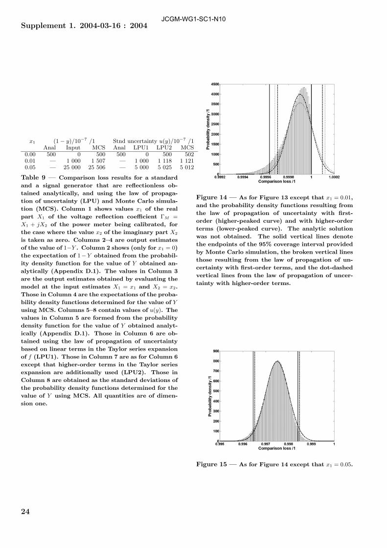
Supplement 1. 2004-03-16 : 2004

x1 (1 − y)/10−7 /1 Stnd uncertainty u(y)/10−7 /1Anal Input MCS Anal LPU1 LPU2 MCS

0.00 500 0 500 500 0 500 5020.01 — 1 000 1 507 — 1 000 1 118 1 1210.05 — 25 000 25 506 — 5 000 5 025 5 012

Table 9 — Comparison loss results for a standard

and a signal generator that are reflectionless ob-

tained analytically, and using the law of propaga-

tion of uncertainty (LPU) and Monte Carlo simula-

tion (MCS). Column 1 shows values x1 of the real

part X1 of the voltage reflection coefficient ΓM =

X1 + jX2 of the power meter being calibrated, for

the case where the value x2 of the imaginary part X2

is taken as zero. Columns 2–4 are output estimates

of the value of 1−Y . Column 2 shows (only for x1 = 0)

the expectation of 1−Y obtained from the probabil-

ity density function for the value of Y obtained an-

alytically (Appendix D.1). The values in Column 3

are the output estimates obtained by evaluating the

model at the input estimates X1 = x1 and X2 = x2.

Those in Column 4 are the expectations of the proba-

bility density functions determined for the value of Y

using MCS. Columns 5–8 contain values of u(y). The

values in Column 5 are formed from the probability

density function for the value of Y obtained analyt-

ically (Appendix D.1). Those in Column 6 are ob-

tained using the law of propagation of uncertainty

based on linear terms in the Taylor series expansion

of f (LPU1). Those in Column 7 are as for Column 6

except that higher-order terms in the Taylor series

expansion are additionally used (LPU2). Those in

Column 8 are obtained as the standard deviations of

the probability density functions determined for the

value of Y using MCS. All quantities are of dimen-

sion one.

Figure 14 — As for Figure 13 except that x1 = 0.01,

and the probability density functions resulting from

the law of propagation of uncertainty with first-

order (higher-peaked curve) and with higher-order

terms (lower-peaked curve). The analytic solution

was not obtained. The solid vertical lines denote

the endpoints of the 95% coverage interval provided

by Monte Carlo simulation, the broken vertical lines

those resulting from the law of propagation of un-

certainty with first-order terms, and the dot-dashed

vertical lines from the law of propagation of uncer-

tainty with higher-order terms.

Figure 15 — As for Figure 14 except that x1 = 0.05.

24

JCGM-WG1-SC1-N10

Supplement 1. 2004-03-16 : 2004

density functions provided by the law of propagation ofuncertainty. These Gaussian probability density func-tions are in turn reasonably close to each other, havingexpectations of 1 − 1.0 × 10−4 and 1 − 1.5 × 10−4 andstandard deviations of 1.0 × 10−4 and 1.1 × 10−4.

Figure 14, for x1 = 0.01, also shows the endpointsof I0.95(Y ) as obtained by the three approaches. Theintervals provided by the law of propagation of uncer-tainty are shifted to the right compared with I0.95(Y ) forMonte Carlo simulation. As a consequence they againinclude infeasible values of Y . The shift is about 70 %of the standard uncertainty. The interval provided byMonte Carlo simulation has its right-hand endpoint atunity, the largest feasible value.

Figure 15, for x1 = 0.05, shows similar information.Now, however, the probability density functions pro-vided by both implementations of the law of propagationof uncertainty are virtually indistinguishable from eachother (a slight “thickening of the curve” at the peak is in-dicative of a region where visually there is a discernibledifference). Further, they are now much closer to theapproximation to the probability density function pro-vided by Monte Carlo simulation. The latter exhibitsa slight skewness, as evidenced in the tail regions. Thecoverage intervals provided by the two variants of thelaw of propagation of uncertainty are visually almostidentical, but still shifted from those for Monte Carlosimulation. The shift is now about 10 % of the stan-dard uncertainty. The intervals provided by the law ofpropagation of uncertainty are now feasible.

NOTES

1 One reason why the law of propagation of uncertaintywith first-order terms (only) might be used in practice isthat software for its implementation is readily available: re-sults obtained from it might sometimes be accepted withoutquestion. For the case where x1 = x2 = 0 (Figure 13),the danger would be apparent because the standard uncer-tainty u(y) was computed as zero, and consequently any cov-erage interval for Y would be of zero length for any coverageprobability. For x1 �= 0 (or x2 �= 0), u(y) and the length ofthe coverage interval for Y are both finite, so no such warningwould be available without prior knowledge of likely values.Thus, a danger in implementing software based on the lawof propagation of uncertainty for these calculations is thatchecks of the software for x1 or x2 sufficiently far from zerowould not indicate obvious problems, although when usedsubsequently in practice for small values of these quantitiesthe results would be invalid, but conceivably unwittingly ac-cepted.

2 The values x1 = x2 = 0 lie in the centre of the regionof interest to the electrical engineer and thus in no senseconstitute an “extreme case” in practice.

The last two rows of Table 9 show the counterparts ofthe quantities in the previous row that apply for the

above values x1 = 0.01 and x1 = 0.05, except that ananalytic solution was not attempted for x1 > 0.

8.3.3 Calculation: correlated input quantities

Consider measurements x1 = 0, 0.01 and 0.05, x2 = 0,with u(x1) = u(x2) = 0.005 and r(x1, x2) = 0.9. ΓM ,the voltage reflection coefficient of the power meter be-ing calibrated, is assigned a bivariate Gaussian proba-bility density function for the values of X1 and X2 withexpectation (x1, 0)T and uncertainty matrix (16)[

0.0052 0.9 × 0.0052

0.9 × 0.0052 0.0052

]. (17)

The probability density function g(η) for the value of Ycan be obtained (a) using the law of propagation of un-certainty with first-order terms, and (b) by Monte Carlosimulation. The law of propagation of uncertainty withsecond-order terms for the case of mutually dependentinput quantities is not treated in the GUM and is notconsidered here.

The basis of the calculations required to implement forthe model (15) the law of propagation of uncertaintywith first-order terms and mutually dependent inputquantities is given in Appendix D.2.2. The standard un-certainty u(y) is evaluated from Expression (21) which,since x2 = 0, reduces to

u2(y) = 4x21u

2(x1).

Consequently, the standard uncertainty does not dependon the value of r(x1, x2) and the law of propagation ofuncertainty with first-order terms gives identical resultsto those presented in Appendix D.2.1. In particular,for the case x1 = 0, the standard uncertainty u(y) iscomputed as zero, as in Subclause 8.3.2.

To implement Monte Carlo simulation (b) it is necessaryto sample randomly from a bivariate Gaussian proba-bility density function with given expectation and un-certainty matrix. The procedure in Appendix C.5 wasused. Results are obtained here for M = 105 trials.

NOTE — Apart from the requirement to sample from a mul-tivariate distribution, the implementation of Monte Carlosimulation for mutually dependent input quantities is nomore complicated than when the input quantities are mu-tually independent (Subclause 8.3.2).

Table 10 contains the results obtained from the the twoapproaches in the cases x1 = 0, 0.01 and 0.05. Theresults obtained from the law of propagation of uncer-tainty using first-order terms are identical to those givenin Table 9. The results obtained from Monte Carlo sim-ulation indicate that although the output estimate y isunaffected by the correlation between input quantities,

25

JCGM-WG1-SC1-N10

Supplement 1. 2004-03-16 : 2004

the standard uncertainty u(y) is influenced by the cor-relation, especially for small x1.

x1 Output quantity value (1 − y)/10−7 u(y)/10−7

From input estimates MCS LPU1 MCS0.00 0 499 0 6720.01 1 000 1 501 1 000 1 2070.05 25 000 25 530 5 000 5 047

Table 10 — As Table 9 but with the following differ-

ences. Columns 2 and 3 are output estimates of the

value of (1−Y )/10−7. The values in Column 2 are the

output estimates obtained by evaluating the model

at the input estimates X1 = x1 and X2 = x2. Those

in Column 3 are the expectations of the probabil-

ity density functions determined for Y using MCS.

Columns 4 and 5 contain values for the standard un-

certainties u(y)/10−7. The values in Column 4 are

obtained using LPU1. Those in Column 5 are ob-

tained as the standard deviations of the distributions

determined for the value of Y using MCS.

Figures 16 and 17 show the probability density func-tions provided by the law of propagation of uncertaintywith first-order terms (bell-shaped curve) and approxi-mated by Monte Carlo simulation (scaled frequency dis-tributions) in the cases x = 0.01 and x = 0.05, respec-tively. The endpoints of the shortest 95 % coverage in-terval I0.95(Y ) provided by the two approaches are alsoshown, as “dash-dot” vertical lines for the law of prop-agation of uncertainty and solid vertical lines for MonteCarlo simulation.

NOTE — Strictly, the conditions under which a Gaussianprobability density function can be assigned do not holdfollowing an application of the law of propagation of un-certainty in this circumstance [GUM 6.2.3]. However, thisprobability density function and the endpoints of the corre-sponding 95 % coverage interval are shown because such anassignment is commonly practised.

In the case x1 = 0.01 (Figure 16) the effect of the cor-relation of the input quantities has been to change no-ticeably the results returned by Monte Carlo simulation(compare with Figure 14). Not only has the “shape”of (the approximation to) the probability density func-tion changed, but the corresponding coverage intervalno longer has its right-hand endpoint at Y = 1. Inthe case x = 0.05, the differences between the resultsfor the correlated and uncorrelated cases (compare withFigure 15) are less obvious.

Figure 16 — Results for the model of comparison

loss in power meter calibration in the case x1 = 0.01,

x2 = 0, with u(x1) = u(x2) = 0.005 and r(x1, x2) = 0.9.

The figure shows the probability density function

(a) provided by the use of the law of propagation of

uncertainty with first-order terms to assign a Gaus-

sian probability density function to the output quan-

tity value (bell-shaped curve), and (b) provided by

Monte Carlo simulation (scaled frequency distribu-

tion) with 105 trials. The “dash-dot” vertical lines

denote the endpoints of the shortest 95 % coverage

interval I0.95(Y ) as derived from the Gaussian prob-

ability density function provided by the law of prop-

agation of uncertainty. The solid vertical lines are

those derived from Monte Carlo simulation.

Figure 17 — As for Figure 16 except that x1 = 0.05.

26

JCGM-WG1-SC1-N10

Supplement 1. 2004-03-16 : 2004

References

[1] R. W. Beatty. Insertion loss concepts. Proc. IEEE,6:663–671, 1964.

[2] P. Mac Berthouex and L. C. Brown. Statistics forEnvironmental Engineers. CRC Press, USA, 1994.

[3] BIPM, IEC, IFCC, ISO, IUPAC, IUPAP, andOIML. Guide to the Expression of Uncertainty inMeasurement, 1995. ISBN 92-67-10188-9, Correctedand reprinted.

[4] BIPM and IEC and IFCC and ISO and IUPAC andIUPAP and OIML. International Vocabulary of Basicand General Terms in Metrology, 1993.

[5] G. E. P. Box and M. Muller. A note on the gener-ation of random normal variates. Ann. Math. Statist.,29:610–611, 1958.

[6] M. G. Cox, M. P. Dainton, and P. M. Harris. Test-ing spreadsheets and other packages used in metrol-ogy. Testing functions for the calculation of standarddeviation. Technical Report CMSC 07/00, NationalPhysical Laboratory, Teddington, UK, 2000.

[7] M. G. Cox, M. P. Dainton, and P. M. Harris. BestPractice Guide No. 6. Uncertainty and statistical mod-elling. Technical report, National Physical Laboratory,Teddington, UK, 2001.

[8] M. G. Cox, M. P. Dainton, and P. M. Harris. Soft-ware specifications for uncertainty evaluation and as-sociated statistical analysis. Technical Report CMSC10/01, National Physical Laboratory, Teddington, UK,2001.

[9] M. G. Cox, M. P. Dainton, P. M. Harris, and N. M.Ridler. The evaluation of uncertainties in the analysisof calibration data. In Proceedings of the 16th IEEEInstrumentation and Measurement Technology Confer-ence, pages 1093–1098, Venice, 24-26 May 1999, 1999.

[10] T.J. Dekker. Finding a zero by means of succes-sive linear interpolation. In B. Dejon and P. Henrici,editors, Constructive Aspects of the Fundamental The-orem of Algebra, London, 1969. Wiley Interscience.

[11] L. Devroye. Non-Uniform Random Number Gener-ation. Springer, New York, 1986.

[12] C. F. Dietrich. Uncertainty, Calibration and Prob-ability. Adam Hilger, Bristol, UK, 1991.

[13] EA. Expression of the uncertainty of measurementin calibration. Technical Report EA-4/02, EuropeanCo-operation for Accreditation, 1999.

[14] EA. Expression of the uncertainty of measurementin calibration. Technical Report EA-4/02, EuropeanCo-operation for Accreditation, 1999.

[15] G. S. Fisher. Monte Carlo. Springer-Verlag, NewYork, 1996.

[16] B. D. Hall. Computer modelling of uncertainty cal-culations with finite degrees of freedom. Meas. Sci.Technol., 11:1335–1341, 2000.

[17] I. A. Harris and F. L. Warner. Re-examinationof mismatch uncertainty when measuring microwavepower and attenuation. Proc. IEEE, 128:35–41, 1981.

[18] I. D. Hill and B. A. Wichmann. Algorithm AS183.An efficient and portable pseudo-random number gen-erator. Appl. Statist., 31:188–190, 1982.

[19] ISO. ISO Guide 35 - Certification of reference ma-terials - general and statistical principles, 1989. Inter-national Standards Organization, Geneva.

[20] ISO. ISO 3534-1:1993. Statistics - Vocabulary andsymbols - Part 1: Probability and general statisticalterms, 1993. International Standards Organization,Geneva.

[21] D. M. Kerns and R. W. Beatty. Basic Theoryof Waveguide Junctions and Introductory MicrowaveNetwork Analysis. Pergamon Press, London, 1967.

[22] A. Kinderman, J. Monahan, and J. Ramage.Computer methods for sampling from Student’s t-distribution. Math. Comput, 31:1009–1018, 1977.

[23] D. E. Knuth. The Art of Computer Programming,Vol. 2: Semi-numerical algorithms. Addison-Wesley,Reading, Ma., USA, 1981.

[24] J. Leydold. Automatic sampling with the ratio-of-uniforms method. ACM Trans. Math. Software, 26:78–98, 2000.

[25] G. Marsaglia. A current view of random numbergenerators. In Computer Science and Statistics: TheInterface, Amsterdam, 1985. Elsevier.

[26] G. Marsaglia and A. Zaman. The KISS generator.Technical report, Department of Statistics, Universityof Florida, USA, 1993.

[27] The MathWorks. Matlab User’s Manual. Math-Works Inc., Natick, Mass., USA, 1992.

[28] M. McCoy. A review on random number gener-ation and methods for generating normal distribu-tions. Technical Report 113/2000, National Engineer-ing Laboratory, UK, 2000.

[29] OIML. Conventional value of the result of weighingin air. Technical Report R 33 - EN, Bureau Interna-tional de Metrologie Legale, Paris, 1979.

[30] J. R. Rice. Mathematical Statistics and Data Anal-ysis. Duxbury Press, Belmont, Ca., USA, second edi-tion, 1995.

[31] N. M. Ridler and M. J. Salter. Propagating S–parameter uncertainties to other measurement quan-tities. In 58th ARFTG (Automatic RF TechniquesGroup) Conference Digest, 2001.

27

JCGM-WG1-SC1-N10

Supplement 1. 2004-03-16 : 2004

[32] B. D. Ripley. Stochastic Simulation. J. Wiley, NewYork, 1987.

[33] C. P. Robert and G. Casella. Monte Carlo Statisti-cal Methods. Springer-Verlag, New York, 1999.

[34] R. Y. Rubenstein. Simulation and the Monte CarloMethod. J. Wiley, New York, 1981.

[35] M. J. Salter, N. M. Ridler, and M. G. Cox. Dis-tribution of correlation coefficient for samples takenfrom a bivariate normal distribution. Technical ReportCETM 22, National Physical Laboratory, Teddington,UK, 2000.

[36] R. S. Scowen. QUICKERSORT, Algorithm 271.Comm. ACM, 8:669, 1965.

[37] G. Strang and K. Borre. Linear Algebra, Geodesyand GPS. Wiley, Wellesley-Cambridge Press, 1997.

[38] B. N. Taylor and C. E. Kuyatt. Guidelines for eval-uating and expressing the uncertainty of NIST mea-surement results. Technical Report TN1297, NationalInstitute of Standards and Technology, 1994.

[39] K. Weise and W. Woger. A Bayesian theory ofmeasurement uncertainty. Measurement Sci. Technol.,3:1–11, 1992.

[40] W. Woger. Probability assignment to system-atic deviations by the Principle of Maximum En-tropy. IEEE Trans. Instr. Measurement, IM-36:655–658, 1987.

28

JCGM-WG1-SC1-N10

Supplement 1. 2004-03-16 : 2004

A Historical perspective

The GUM is a rich document, covering many aspects ofuncertainty evaluation. Although it does not refer ex-plicitly to the use of Monte Carlo simulation, this optionwas recognized during the drafting of the GUM. TheISO/IEC/OIML/BIPM draft (First Edition) of June1992, produced by ISO/TAG 4/WG 3, states, as Sub-clause G.1.5:

If the relationship between Y [the output mea-surand] and its input quantities is non-linear, or ifthe values available for the parameters character-izing the probabilities of the Xi [the input quan-tities] (expectation, variance, higher moments) areonly estimates and are themselves characterized byprobability distributions, and a first order Taylorexpansion is not an acceptable approximation, thedistribution of Y cannot be expressed as a convo-lution. In this case, numerical methods (such asMonte Carlo calculations) will generally be requiredand the evaluation is computationally more diffi-cult.

In the published version of the GUM [3], this subclausehad been modified to read:

If the functional relationship between Y and itsinput quantities is non-linear and a first-order Tay-lor expansion is not an acceptable approximation(see 5.1.2 and 5.1.5), then the probability distri-bution of Y cannot be obtained by convolving thedistributions of the input quantities. In such cases,other analytical or numerical methods are required.

The interpretation made here of this re-wording is that“other analytical or numerical methods” cover any otherappropriate approach. This interpretation is consistentwith that of the National Institute of Standards andTechnology of the United States [38]:

[Clause 6.6] The NIST policy provides for excep-tions as follows (see Appendix C):

It is understood that any valid statistical methodthat is technically justified under the existing cir-cumstances may be used to determine the equiva-lent of ui [the standard deviation of the ith inputquantity], uc [the standard deviation of the outputquantity], or Up [the half-width of a coverage inter-val for the output measurand value, under a Gaus-sian assumption]. Further, it is recognized that in-ternational, national, or contractual agreements towhich NIST is a party may occasionally require de-viation from NIST policy. In both cases, the reportof uncertainty must document what was done andwhy.

Further, within the context of statistical modelling inanalyzing the homogeneity of reference materials, it isstated within ISO Guide 35 [19]:

[Subclause 9.2.3] ... where lack of a normal distri-bution is a problem, robust or non-parametric sta-tistical procedures may be used to obtain a validconfidence interval for the quantity of interest.

29

JCGM-WG1-SC1-N10

Supplement 1. 2004-03-16 : 2004

B Sensitivity coefficients

Neither the propagation of distributions nor its imple-mentation using Monte Carlo simulation provides sen-sitivity coefficients [GUM 5.1.3], for two reasons. First,sensitivity coefficients are not an inherent part of thepropagation of distributions. Second, for a non-linearmodel, sensitivity coefficients are in general approxi-mate. However, simply by holding all input quantitiesbut one fixed at their best estimates, Monte Carlo sim-ulation can be used to provide the probability densityfunction for the output quantity value for the modelhaving just that input quantity as a variable [7]. Theratio of the standard deviation of this probability den-sity function and that of the relevant input quantitycan be taken as a sensitivity coefficient. This value cor-responds to that which would be obtained by taking allhigher-order terms in the Taylor series expansion of themodel into account. In the case of complicated mod-els this approach can be used as a practical alternativeto the “tedious analysis” required to provide sensitivitycoefficients [16].

The sensitivity coefficients so obtained must not gen-erally be taken in conjunction with the standard un-certainties associated with the best estimates of the in-put quantities as the only contributions to the standarduncertainty associated with the output quantity value.There will be further contributions arising from any in-teraction (i.e., non-additive) terms in the model.

30

JCGM-WG1-SC1-N10

Supplement 1. 2004-03-16 : 2004

C Sampling from probability distribu-tions

This appendix provides some technical information con-cerning sampling from probability distributions. Suchsampling forms a central part of the use of Monte Carlosimulation as an implementation of the propagation ofdistributions for uncertainty evaluation.

C.1 General distributions

It is possible to provide a sample z from any continu-ous distribution function G(η) by transforming a samplefrom a rectangular distribution:

a) Sample a random number ψ from the rectangulardistribution U [0, 1].

b) Find the value z satisfying G(z) = ψ.

NOTES

1 The “inversion” required in Step b), i.e., forming z =G−1(ψ), may be possible analytically. Otherwise it can becarried out numerically.

2 As an as example of an analytic inversion, consider theexponential probability density function with expectation x,viz., g(ξ) = exp(−ξ/x)/x, for ξ ≥ 0, and zero otherwise(Clause 4.1). Then G(ξ) = 1− exp(ξ/x), for ξ ≥ 0, and zerootherwise. Hence z = −x loge(1 − ψ).

3 Numerically, z can generally be determined by solvingthe “zero-of-a-function” problem G(z) − ψ = 0. Upper andlower bounds for z are typically easily found, in which case arecognised “bracketing” algorithm such as bisection or, moreefficiently, a combination of linear interpolation and bisec-tion [10], for example, can be used to determine z.

Emphasis is given here to the commonest distributions.

C.2 Rectangular distribution

The ability to generate pseudo-random numbers froma (continuous) rectangular distribution is fundamentalin its own right, and also as the basis for generatingpseudo-random numbers from any distribution (aboveand Appendices C.3 and C.4). using an appropriate al-gorithm or formula. In the latter regard, the quality ofthe numbers generated from a non-rectangular distribu-tion depends on that of the rectangular generator and onthe properties of the algorithm employed. The quality ofthe non-rectangular generator can therefore be expectedto be correlated with that of the rectangular generator.Only a good rectangular generator and a good algorithmcan be expected to provide a good non-rectangular gen-erator. It is thus important that the underlying rect-angular generator is sound (cf. [24]). Unless the user is

sure of the pedigree of a rectangular generator it shouldnot be used until adequate testing has been carried out.Invalid results can otherwise be obtained. Some of the“tests for randomness” that should be undertaken areindicated below. A recommended rectangular genera-tor, that has been shown to perform well in these testsand that is straightforward to implement, is given in thisappendix.

Table C.1 defines relevant aspects of the functioning ofa procedure for generating rectangular pseudo-randomnumbers in the interval [0, 1], specifying the input,input-output and output parameters associated withtheir determination.

Input parameters

q Number of rectangular pseudo-random numbers tobe generated

Input-output parameters

t Column vector of parameters required as input quan-tities and that may be changed as part of the compu-tation. The subsequent values of these quantities arenot usually of immediate concern to the user. Theparameters are needed to help control the processby which the pseudo-random numbers are produced.The parameters may be realized as global variablesand thus not explicitly appear as parameters of theprocedure. One or more of these parameters may bea seed, used to initiate the sequence of random num-bers produced by successive calls of the procedure.By setting the seeds to values previously used, thesame sequence of random numbers can be produced.Doing so is important as part of software regressiontesting, used to verify the consistency of results pro-duced using the software with those from previousversions

Output parameters

z q “draws” from a variable rectangularly distributedbetween zero and one

Table C.1 — Rectangular pseudo-random number

generation.

A rectangular pseudo-random number x in the inter-val [a, b] can be formed by determining a + (b − a)z,where z is a rectangular pseudo-random number in theinterval [0, 1].

C.2.1 Randomness tests

A review [28] has been carried out of the use of randomnumbers in solving problems using Monte Carlo simu-lation. It draws conclusions concerning, in particular,the best methods to employ for generating rectangularpseudo-random numbers. The so-called “combinationgenerators” are recommended and are reported as be-ing favoured by experts as fulfilling the requirements ofpossessing the longest periods and passing a set of sta-tistical tests for randomness.

31

JCGM-WG1-SC1-N10

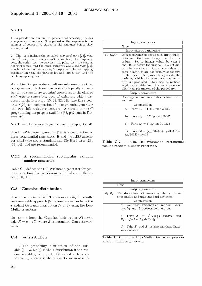
Supplement 1. 2004-03-16 : 2004

NOTES

1 A pseudo-random number generator of necessity providesa sequence of numbers. The period of the sequence is thenumber of consecutive values in the sequence before theyare repeated.

2 The tests include the so-called standard tests [23], viz.,the χ2 test, the Kolmogorov-Smirnov test, the frequencytest, the serial test, the gap test, the poker test, the couponcollector’s test, and the more stringent Die Hard tests [25],which include the overlapping M -tuple test, the overlappingpermutation test, the parking lot and lattice test and thebirthday-spacing test.

A combination generator simultaneously uses more thanone generator. Each such generator is typically a mem-ber of the class of congruential generators or the class ofshift register generators, both of which are widely dis-cussed in the literature [15, 23, 32, 34]. The KISS gen-erator [26] is a combination of a congruential generatorand two shift register generators. A version in the Cprogramming language is available [33, p42] and in For-tran [26].

NOTE — KISS is an acronym for Keep It Simple, Stupid!

The Hill-Wichmann generator [18] is a combination ofthree congruential generators. It and the KISS genera-tor satisfy the above standard and Die Hard tests [28],[33, p41] and are recommended.

C.2.2 A recommended rectangular randomnumber generator

Table C.2 defines the Hill-Wichmann generator for gen-erating rectangular pseudo-random numbers in the in-terval [0, 1].

C.3 Gaussian distribution

The procedure in Table C.3 provides a straightforwardlyimplementable approach [5] to generate values from thestandard Gaussian distribution N(0, 1) using the Box-Muller transform.

To sample from the Gaussian distribution N(µ, σ2),take X = µ + σZ, where Z is a standard Gaussian vari-able.

C.4 t–distribution

. . . The probability distribution of the vari-able (ζ − µζ)/s(ζ) is the t–distribution if the ran-dom variable ζ is normally distributed with expec-tation µζ , where ζ is the arithmetic mean of n in-

Input parameters

None

Input-output parameters

iA, iB , iC Integer parameters required as input quan-tities and that are changed by the pro-cedure. Set to integer values between 1and 30000 before the first call. Do not dis-turb between calls. Subsequent values ofthese quantities are not usually of concernto the user. The parameters provide thebasis by which the pseudo-random num-bers are produced. They may be realisedas global variables and thus not appear ex-plicitly as parameters of the procedure

Output parameters

Z Rectangular random number between zeroand one

Computation

a) Form iA = 171iA mod 30269

b) Form iB = 172iB mod 30307

c) Form iC = 170iC mod 30323

d) Form Z = (iA/30269 + iB/30307 +iC/30323) mod 1

Table C.2 — The Hill-Wichmann rectangular

pseudo-random number generator.

Input parameters

None

Output parameters

Z1, Z2 Two draws from a Gaussian variable with zeroexpectation and unit standard deviation

Computation

a) Generate rectangular random vari-ates V1 and V2 between zero and one

b) Form Z1 =√−2 log V1 cos 2πV2 and

Z2 =√−2 log V1 sin 2πV2

c) Take Z1 and Z2 as two standard Gaus-sian variates

Table C.3 — The Box-Muller Gaussian pseudo-

random number generator.

32

JCGM-WG1-SC1-N10

Supplement 1. 2004-03-16 : 2004

dependent observations ζi of ζ, s(ζi) is the exper-imental standard deviation of the n observations,and s(ζ) = s(ζi)/

√n is the experimental standard

deviation of the arithmetic mean ζ with ν = n − 1degrees of freedom. [GUM C.3.8]

The procedure in Table C.4 provides an approach [22],[33, p63] to generate values from the t–distributionwith ν degrees of freedom, which is also straightforwardto implement. Full details are available [22].

Input parameters

ν Degrees of freedom

Output parameters

Z Draw from a t–distribution with ν degrees of free-dom

Computation

a) Generate rectangular random variates V1

and V2 between zero and one

b) If V1 < 1/2, set Z = 1/(4V1 − 1) and V =V2/Z

2; otherwise set Z = 4V1 − 3 and V = V2

c) If V < 1−|Z|/2 or V < (1+Z2/ν)−(ν+1)/2,accept Z as a t-distribution variate; otherwiserepeat from Step C.4a

Table C.4 — A t–distribution pseudo-random num-

ber generator.

For an expectation µ and standard deviation σ and νdegrees of freedom, take X = µ+σT , where T is a vari-able having a t–distribution with ν degrees of freedom.

Sampling from the t–distribution can be used in MonteCarlo simulation when synthesizing probability densityfunctions assigned to input quantities represented by re-peated observations that can be regarded as drawn froma Gaussian distribution.

NOTE — This use has been criticized in some quarters inthat coverage intervals determined for the output quantityvalue can be pessimistically long. Conversely, were a Gaus-sian probability density function assigned, i.e., with no ac-count taken of the degrees of freedom that the t–distributionis intended to accommodate, the resulting coverage intervalscould be optimistically short. This matter remains a re-search topic. It is recommended that a decision is agreedand recorded with the details of the uncertainty evaluationin any one instance. In particular, despite the statement inthe GUM that uncertainty evaluations should be realistic,if in doubt it might be wiser and certainly cautious to usethe t–distribution, accompanying the results of uncertaintyevaluation by a suitable qualifying statement.

C.5 Multivariate Gaussian distribution

The most important multivariate distribution is themultivariate Gaussian distribution. An n × 1 vector ofexpectations µ and an uncertainty matrix V of order ndefine the parameters of the n-dimensional Gaussian dis-tribution.

Values can be sampled from this multivariate (or joint)Gaussian distribution [35, 37] using the procedure inTable C.5.

Input parameters

n Dimension of the multivariate Gaussian distribu-tion

µ n × 1 vector of expectationsV Uncertainty matrix of order nq Number of multivariate Gaussian pseudo-random

numbers to be generated

Output parameters

X An n×q matrix, the jth column of which is a drawfrom the multivariate Gaussian distribution

Computation

a) Form the Cholesky factor R of V , i.e., theupper triangular matrix satisfying V = RTR.(To generate q pseudo-random numbers it is nec-essary to perform this matrix factorization onlyonce.)

b) Form q samples from the n-dimensionalstandard Gaussian distribution N(0, 1) × . . . ×N(0, 1). Here, N(µ, σ2) denotes the Gaussiandistribution with expectation µ and standarddeviation σ. Doing so simply means generatingan n × q array Z of standard Gaussian variates

c) Provide the required sample (the Choleskyfactor acts as a transformation from the uncor-related standardized space to that required):

X = µE + RTZ ,

where E denotes a row vector of q ones

Table C.5 — A multivariate Gaussian random num-

ber generator.

Figure C.1 shows 200 points generated from a bivariateGaussian distribution, using the MULTNORM genera-tor [35], with expectation µ = (2, 3)T and uncertaintymatrix

V =[

2.0 1.91.9 2.0

].

Similar generators are available elsewhere [11].

In this figure the points “span” an elongated angled el-lipse. Were the off-diagonal elements of V to be re-placed by zero, the points would span a circle. Were thediagonal elements made unequal, and the off-diagonalelements kept at zero, the points would span an ellipse

33

JCGM-WG1-SC1-N10

Supplement 1. 2004-03-16 : 2004

Figure C.1 — Points sampled from a bivariate

Gaussian distribution with positive correlation.

whose axes were parallel to the axes of the graph.

34

JCGM-WG1-SC1-N10

Supplement 1. 2004-03-16 : 2004

D The comparison loss problem

D.1 The analytic solution for a zero valueof the voltage reflection coefficient

For the case x1 = x2 = r(x1, x2) = 0 and u(x1) = u(x2),the probability density function g(η) (Subclause 8.3.1)can be obtained analytically. It is valuable to have sucha solution for validation purposes, even though in othercases this may not be possible. The model Y = 1−X2

1 −X2

2 can be expressed in the above circumstances as

Y = 1 − u2(x1){X21/u2(x1) + X2

2/u2(x2)}.The term in braces is the sum, Z, say, of the squares oftwo mutually independent standard normal probabilitydensity functions, and is therefore distributed as χ2 withtwo degrees of freedom [30, p177]. Thus,

Y = 1 − u2(x1)Z.

Y is a differentiable and strictly monotonic functionof Z. The application of a general formula [7, For-mula (5.1)], [30, pp57–61] for the probability densityfunction g(η) of a function of a variable with a specifiedprobability density function hence yields

g(η) = χ22(Z)/u2(x1),

where χ2ν(Z) is χ2 in Z with ν degrees of freedom.

Since [30, pp177-178]

χ2ν(Z) =

Zν/2−1e−Z/2

2ν/2Γ(ν/2),

where here, as opposed to Clause 8.3, Γ denotes thegamma function, the required probability density func-tion is

g(η) = exp(−(1 − η)/(2u2(x1)))/(2u2(x1)), η ≤ 1.

The expectation is straightforwardly shown to be

E(η) =∫ 1

−∞ηg(η)dη = 1 − 2u2(x1)

and the variance∫ 1

−∞(η − E(η))2g(η)dη = 4u4(x1),

i.e., the standard deviation is 2u2(x1).

The corresponding distribution function is given by in-tegration as

G(η) = exp(−(1 − η)/(2u2(x1))), η ≤ 1. (18)

A 95 % coverage interval I0.95(Y ) for the output quan-tity value is then (Clause 6.7)

[G−1(p), G−1(p + 0.95)],

for any p satisfying 0 ≤ p ≤ 0.05. The shortest I0.95(Y )is given by the value of p that minimizes H(p) ≡G−1(p+0.95)−G−1(p). Let yp be the value of Y in (18)corresponding to G(η) = p. Simple algebra gives

yp = 1 + 2u2(x1) log p.

Hence

I0.95(Y ) = [1 + 2u2(x1) log p, 1 + 2u2(x1) log(p + 0.95)]

and

H(p) = 1 + 2u2(x1) log(p + 0.95) − (1 + 2u2(x1) log p),

which simplifies to

H(p) = 2u2(x1) log(1 + 0.95/p),

a decreasing function of p. Since p is to satisfy 0 ≤ p ≤0.05, H(p) is minimized when p = 0.05. Thus,

I0.95(Y ) = [1 + 2u2(x1) log 0.05, 1]

which, expressed as a coverage interval for 1 − Y , is

I0.95(1 − Y ) = [0,−2u2(x1) log 0.05].

For the above value of u(x1) = 0.005,

I0.95(1 − Y ) = [0, 0.0001498].

For comparison, the 95 % coverage interval that is sym-metric with respect to probability (Clause 6.7) is

I0.95(1 − Y ) = [−2u2(x1) log(p + 0.975),− 2u2(x1) log(p + 0.025)]

= [0.0000039, 0.0001844],

which is 20 % longer than the shortest interval.

NOTE — The above analysis is indicative of an analyticapproach that can be applied to some problems of this type.In this particular case, the results could in fact have beenobtained more directly, based on the observation that g(η) ismonotonically increasing and using the fact that the shortestcoverage interval is always in the region of highest density.

D.2 The law of propagation of uncertaintyapplied to the comparison loss prob-lem

D.2.1 Uncorrelated input quantities

The comparison loss problem considered in Clause 8.3has as the mathematical model of measurement

Y = f(X) = f(X1, X2) = 1 − X21 − X2

2 ,

where the values of X1 and X2 are assigned Gaus-sian probability density functions with expectations x1

and x2 and variances u2(x1) and u2(x2), respectively.

35

JCGM-WG1-SC1-N10

Supplement 1. 2004-03-16 : 2004

The application of GUM Subclause 5.1.1 gives

y = 1 − x21 − x2

2

as the estimate of the output quantity value. The onlynon-trivially nonzero partial derivatives of the modelare, for i = 1, 2,

∂f/∂Xi = −2Xi, ∂2f/∂X2i = −2.

Hence the application of GUM Subclause 5.1.2 gives, asthe standard uncertainty u(y),

u2(y) =(

∂f

∂X1

)2∣∣∣∣∣X=x

u2(x1)

+(

∂f

∂X2

)2∣∣∣∣∣X=x

u2(x2)

= 4x21u

2(x1) + 4x22u

2(x2), (19)

based on a first-order Taylor series approximationof f(X). If the non-linearity of f is significant, theterm

12

{(∂2f

∂X21

)2

+(

∂2f

∂X22

)2}∣∣∣∣∣

X=x

u2(x1)u2(x2)

must be appended to Formula (19), in which case For-mula (19) becomes

u2(y) = 4x21u

2(x1) + 4x22u

2(x2) + 4u2(x1)u2(x2). (20)

A 95 % coverage interval for Y is then given by

y ± 2u(y),

as a consequence of the assumption that Y has a Gaus-sian probability density function.

D.2.2 Correlated input quantities

The extension of the comparison loss problem to mu-tually dependent input quantities is considered. Thechanges necessary to the above treatment are given. Theuncertainty matrix for the input quantities is given inFormula (16), where the correlation coefficient r(x1, x2)is specified and in general takes a nonzero value.

The application of GUM Subclause 5.2.2 gives

u2(y) = (∂f/∂X1)2u2(x1) + (∂f/∂X2)2u2(x2)+ 2(∂f/∂X1)(∂f/∂X2)r(x1, x2)u(x1)u(x2)= 4x2

1u2(x1) + 4x2

2u2(x2)

+ 8r(x1, x2)x1x2u(x1)u(x2), (21)

based on a first-order Taylor series approximationof f(X), where all derivatives are evaluated at X = x.

36

JCGM-WG1-SC1-N10

Indexassociated standard uncertainty, see §3

best estimate, 2, see §Bof input quantity value, see §1, see §3, see §8.1.1,

see §8.1.2, see §Bof output quantity value, see §1, see §2, see §3, see

§6.6, see §6.10, see §7, see §D.2.1

Central Limit Theorem, see §2, see §1, see §6, see §7,see §8.1.3

correlated input quantities, see §D.2.2correlation coefficient between best estimates, see

§8.3.1covariances of best estimates, see §3, see §8.3.1coverage

factor, see §6.7, see §8.1.1, see §8.1.3interval, 2, see §1, see §2, see §3, see §6, see §6.2,

see §6.6, see §6.7, see §6.8, see §6.10, see §7,see §8.1.1, see §8.1.3, see §8.1.2, see §8.2.2,see §8.1.3, see §8.2.2, see §8.3.1, see §8.3.2, see§8.3.3, see §A, see §C.4, see §D, see §D.2.1

probability, see §1, see §3, see §6, see §6.2, see §6.7,see §6.8, see §7, see §8.2.2, see §8.3.2

degree of belief, 2degrees of freedom, see §1, see §3, see §4.1, see §6.2,

see §6.6, 33, see §C.4, 35, see §Deffective, 3, see §3

distributionCauchy, see §1frequency, 2, see §6.5, see §8.1.1, see §8.2.2, see

§8.3.2, see §8.3.3function, see §2, see §4, see §4.2, see §6, 11, see

§6.5, see §6.6, see §6.7, see §8.1.1Gaussian, see §6.3, see §8.2.1, see §8.3.2, 32, see

§C.3, 33, see §C.5, see §C.4multivariate Gaussian, see §6.3, see §C.5normal, see §8.1.1, see §A, 32rectangular, see §6.3, see §8.1.2, see §8.1.3, see

§8.2.1, 31, see §C.1, see §C.2sampling from Gaussian, see §8.3.3, see §C.5Student’s-t, see §C.4

expectation, see §3

input quantitiesmutually dependent, see §1, see §3, see §6, see

§8.3.3, see §D.2.2mutually independent, see §1, see §6, see §8.2.1,

see §8.3.3

measurement modelcalibration of mass standards, see §8.2.1calibration of microwave power meter, see §D.2.1

model, see §3

Monte Carlo simulation, 2, see §4.2, see §5, see §6, see§6.5, see §6.4, see §6.3, see §6.2, see §6.5, see§6.10, see §6.9, see §7, see §8, see §8.1.1, see§8.1.3, see §8.1.2, see §8.2.2, see §8.1.3, see§8.2.2, see §8.3.2, see §8.3.1, see §8.3.2, see§8.3.3, see §8.3.2, see §8.3.3, see §A, see §B,see §C, see §C.2.1, see §C.4

adaptive procedure for, see §6.10computation time for, see §6.9number of trials, see §6.2, see §6.10, see §6.8, see

§6.10

partial derivative, see §1, see §3, see §8.2.2, see §8.3.2,see §D.2.1

probability density function, 2, see §2, see §1, see §3,see §4, see §3, see §4.2, see §5, see §6, see §5,see §6.4, see §6.3, see §6.5, see §6.7, see §6.9,see §8.1.1, see §8.1, see §8.1.1, see §8.1.2, see§8.1.3, see §8.1.2, see §8.2.2, see §8.2.1, see§8.1.3, see §8.2.2, see §8.3.2, see §8.3.1, see§8.3.2, see §8.3.3, see §8.3.2, see §8.3.3, see§B, see §C.1, see §C.4, see §D, see §D.2.1

assigned to input quantity value, see §1, see §3, see§4.1, see §4, see §5, see §6, see §6.3, see §6.6,see §6.9, see §8, see §C.4

asymmetric, 2, see §1, see §6.7, see §8.1.1expectation of, see §1, see §3, 8, see §4.2, see §6, see

§6.5, see §6.6, see §8.1, see §8.1.2, see §8.3.2for output quantity value, approximation of, 2, see

§1, see §3, see §6.2, see §8.1.1, see §8.1.3, see§8.2.2

joint, see §1, see §3, see §6sampling from, see §6, see §8.1.1standard deviation of, see §1, see §3, see §4.2, see

§6.5, see §8.1, see §8.1.2, see §8.1.3, see §8.1.2,see §8.3.2, see §B

symmetric, see §8.1.1probability distribution

analytical propagation of, see §8.3.2propagation of, 2, see §1, see §4, 8, see §5, see §6,

see §7propagation of uncertainty

law of, 2, see §1, see §2, see §1, see §3, see §4, see§5, see §6.4, see §6.7, see §7, see §8, see §8.1.1,see §8.1.2, see §8.2.2, see §8.3.2, see §8.3.1, see§8.3.2, see §8.3.3, see §8.3.2, see §8.3.3

validation of law of, see §1, see §3, see §5, see §7,see §8, see §8.1.1, see §8.1.3, see §8.1.2, see§8.2.2

random numbers, see §C.2.1, see §C.2pseudo, see §C.2.1, see §C.2, see §C.2.2, see §C.5

rectangular number generatorquality of, see §C.2randomness test of generator, see §C.2

37

JCGM-WG1-SC1-N10

Supplement 1. 2004-03-16 : 2004

recommended, see §C.2.2

sensitivity coefficients, see §1, see §3, see §8.2.2, see §Bshortest length of coverage interval, see §8.1.1significant digits, no. of, see §1, see §6.8, see §7, see

§8.1.1, see §8.1.3, see §8.1.2, see §8.2.2sorting algorithm, see §6.5stages of evaluation, formulation, see §4standard deviation, see §3

Taylor series approximation, 4, see §2, see §3, see §5,see §7, see §8, see §8.3.2, see §B, see §D.2.2,see §D.2.1

uncertainty evaluation problems, see §1uncertainty matrix, see §4.1, 8, see §8.3.2, see §8.3.1,

25, see §8.3.3, see §C.5, see §D.2.2uncertainty of input quantity value, standard, see §Buncertainty of measurement

combined, see §2evaluation of, 2expanded, 3, see §3

Welch-Satterthwaite formula, see §1, see §3, see §7

38

JCGM-WG1-SC1-N10