Guidance on how aged sorption studies for pesticides should be conducted, analysed and used in regulatory

assessments

Final version October 2019

Page 2 of 78

Table of contents

Table of contents ............................................................................................................................................... 2

Preface............................................................................................................................................................... 4

Revision September 2016 ................................................................................................................................. 5

Revision October 2019 ...................................................................................................................................... 5

1 Introduction ................................................................................................................................................... 7

2 Modelling of aged sorption and conceptual definition of equilibrium sorption .............................................. 7 2.1 Modelling of aged sorption................................................................................................................. 7 2.2 Conceptual definition of equilibrium sorption ..................................................................................... 8

3 Experiments to derive aged sorption parameters ........................................................................................ 8 3.1 Soil selection and preparation ........................................................................................................... 9 3.2 Sample preparation and incubation ................................................................................................. 10 3.3 Extraction and analysis .................................................................................................................... 10 3.4 Special considerations for legacy studies ........................................................................................ 11

4 Fitting of kinetic models to data from aged sorption studies ...................................................................... 12 4.1 Data issues ...................................................................................................................................... 12

4.1.1 Data requirements for new studies ...................................................................................... 12 4.1.2 Data requirements for legacy studies .................................................................................. 12 4.1.3 Data handling ...................................................................................................................... 12 4.1.4 Outliers ................................................................................................................................ 13

4.2 Models ............................................................................................................................................. 13 4.3 Tools ................................................................................................................................................ 16

4.3.1 PEARLNEQ ......................................................................................................................... 18 4.3.2 ModelMaker 4.0 ................................................................................................................... 18 4.3.3 MatLab ................................................................................................................................. 19

4.4 Optimisation procedure .................................................................................................................... 19 4.4.1 Variables used in the optimisation. ...................................................................................... 19 4.4.2 Fitted parameters ................................................................................................................ 20 4.4.3 Optimisation settings ........................................................................................................... 20 4.4.4 Starting values ..................................................................................................................... 22 4.4.5 Parameter ranges ................................................................................................................ 23 4.4.6 Weighting ............................................................................................................................. 23

4.5 Goodness of fit criteria ..................................................................................................................... 24 4.5.1 Visual assessment of model fit ............................................................................................ 25 4.5.2 Visual assessment of weighted residuals ........................................................................... 26 4.5.3 Chi

2-test for assessing the goodness of fit .......................................................................... 27

4.6 Evidence for aged sorption .............................................................................................................. 28 4.7 Criteria for the acceptability of the fitted parameters ....................................................................... 29

4.7.1 Confidence intervals and relative standard error ................................................................ 29 4.7.2 Correlation coefficients ........................................................................................................ 29

5 Aged sorption in the tiered pesticide leaching assessment ....................................................................... 30 5.1 Sorption and degradation endpoints from aged sorption studies .................................................... 30

5.1.1 Alternative ways of estimating aged sorption parameters................................................... 32 5.2 Use of aged sorption study data at lower tier .................................................................................. 32 5.3 Combining lower-tier and higher-tier data ....................................................................................... 32

5.3.1 Calculating average sorption parameters ........................................................................... 33 5.3.2 Calculating the average aged-sorption parameters ............................................................ 34 5.3.3 Estimating DegT50EQ values from lower-tier DegT50 values.............................................. 34 5.3.4 Calculating average degradation endpoints ........................................................................ 37

5.4 Groundwater modelling .................................................................................................................... 40

6 Special considerations for metabolites ....................................................................................................... 41

Page 3 of 78

7 References ................................................................................................................................................. 42

Appendix 1. Glossary ....................................................................................................................................... 44

Appendix 2: Fitting of a two-site model with PEARLNEQ to two example datasets ....................................... 47

Appendix 3: Combining degradation and sorption data from Tier 1 and aged sorption studies – example cases .......................................................................................................................................................... 62

Appendix 4: Uncertainty review ....................................................................................................................... 63 A4.4 References ......................................................................................................................................... 67

Appendix 5: The Freundlich Exponent ............................................................................................................ 68 A5.5 References ......................................................................................................................................... 68

Appendix 6: Research on the use of field data for aged sorption in regulatory leaching assessments .......... 70 A6.1 Background ........................................................................................................................................ 70 A6.2 Methods ............................................................................................................................................. 70 A6.3 Recommendations for method 1 ........................................................................................................ 70 A6.4 Recommendations for Method 2 ........................................................................................................ 72 A6.5 Soil properties and weather conditions .............................................................................................. 73 A6.6 References ......................................................................................................................................... 75

Appendix 7: Research on the use of metabolite data to generate aged sorption parameters for regulatory leaching assessments ................................................................................................................................ 76 A7.1 Background ........................................................................................................................................ 76 A7.2 Metabolite-dosed studies ................................................................................................................... 76 A7.3 Parent-dosed studies ......................................................................................................................... 76 A7.4 References ......................................................................................................................................... 78

Page 4 of 78

Preface

Adsorption of chemicals to soil constituents can significantly influence their availability to non-target soil organisms and their potential to move to groundwater or surface waters. Within the regulatory risk assessment procedure for pesticides, first tier assessments currently assume that pesticide sorption is instantaneous and fully reversible, and that strength of adsorption is therefore constant with time. However, adsorption has frequently been observed to increase as the time of interaction between substances and soil also increases. This phenomenon has been given a variety of names, including ‘aged sorption’, ‘time dependent sorption’, ‘increase in sorption over time’, ‘kinetic sorption’ and ‘’non-equilibrium sorption’. As a result of these observations, it is becoming more common for experimental studies that demonstrate an increase in pesticide sorption with time to be submitted to regulatory authorities as part of the regulatory data package. The results of these studies are then used by applicants to revise estimates of predicted environmental concentrations in groundwater. However, such studies are complex and the results are often difficult to interpret. There is currently a lack of agreed and clear guidance on acceptable study methodologies, interpretation of these higher tier studies and the consequent implementation of results in regulatory exposure assessments. Having received a number of regulatory submissions containing studies investigating aged sorption and being aware that other regulatory authorities were in a similar position, the UK Chemicals Regulation Directorate (CRD) recognised that there was a need for regulatory guidance in this area. CRD therefore commissioned a project (funded by Defra and jointly undertaken by the Food and Environment Research Agency (FERA) in the UK and by Alterra in the Netherlands), to investigate aged sorption of pesticides. The project had a number of specific objectives:

To review model concepts and experimental techniques to characterise time-dependent sorption.

To measure time dependent sorption in laboratory studies for a range of soils and pesticides using various experimental techniques.

To derive model input parameters from the experimental data and evaluate the effect of the experimental methodology, data handling and parameter estimation techniques on the results.

To develop and disseminate the guidance on how aged sorption studies should be conducted, analysed and used in regulatory assessments.

The project was wide-ranging and based on literature review, experimental work and extensive modelling to investigate the most suitable approaches for assessing aged sorption of pesticides. It concluded that a two-site conceptual model of aged sorption was considered to be the best option for use in regulatory leaching models. This type of model is the most common mathematical description of time-dependent sorption that is currently used in the regulatory context and, additionally, is integrated into the most recent FOCUS versions of the pesticide leaching models PEARL, MACRO, PELMO and PRZM (EC, 2014a). A sensitivity analysis also demonstrated that the results of leaching assessments are very sensitive to changes in aged sorption parameters, showing the vital importance of determining reliable modelling input parameters. A guidance document was drafted based on the findings of the research project to set out proposed procedures for measuring aged sorption, the derivation of sorption parameters and the use of these parameters in the regulatory risk assessment. The proposed guidance was presented to, and discussed by, an audience of invited representatives of European regulatory authorities, academia, consultancies and industry at a workshop held in April 2010. Feedback was collated from a number of breakout groups and plenary discussions, where a range of specific questions relating to the guidance were presented to the delegates. Following the workshop, member companies of the European Crop Protection Association (ECPA) offered to provide a number of data sets on pesticide substances for the purpose of testing the guidance document. The evaluation of these data was performed by an independent consultancy, Battelle UK Ltd, and subsequently peer reviewed by the FERA research team. The results of this evaluation and peer review, along with the comments from the workshop, have been incorporated into the revised guidance document presented here. The evaluation of aged sorption and derivation and incorporation of aged sorption parameters into regulatory assessments for pesticides is detailed and complex. As a consequence, this guidance is only able to deal with aged sorption as investigated in laboratory studies on directly dosed substances. The estimation of

Page 5 of 78

aged sorption parameters for metabolites formed from dosed parent substances and for substances in field dissipation studies are potentially much more complex and have not been able to be addressed by the research effort forming the basis of this guidance. It is hoped that this guidance will prove to be useful to applicants and regulatory authorities in conducting aged sorption studies, deriving aged sorption parameters for use in regulatory models and the conduct of environmental exposure assessments using these parameters. Andy Massey and James Hingston Chemicals Regulation Directorate, May 2012 Acknowledgements The following are gratefully acknowledged: Sabine Beulke and Wendy van Beinum of Enviresearch (previously FERA) for writing the earlier versions of this guidance; Jos Boesten and Mechteld ter Horst of Alterra for advice; ECPA members for provision of aged sorption data and comments on the draft guidance; Ian Hardy of Battelle (UK) Ltd for the evaluation of ECPA aged sorption data sets and comments on the draft guidance; participants of the workshop held in April 2010; members of the EFSA working group on Aged Sorption and the EFSA PPR panel (2015; 2018) for their dedicated review of the proposed guidance; and European Crop Protection Association for funding the further research and revisions and for assisting in the collation of additional data.

Revision September 2016

The proposed guidance on aged sorption was reviewed by the EFSA PPR panel and ad hoc Working Group on Aged Sorption during 2014-2015. Following the review, EFSA published a Statement on the aged sorption guidance in July 2015. In the Statement, the EFSA PPR panel agreed in general with the experimental and modelling approaches that were proposed in the guidance. Some revisions of the guidance were requested regarding the interpretation of aged sorption data, and how the data is used in the tiered risk assessment. Additional testing on ‘real world data’ was requested for some of the proposed changes.

The guidance was revised in September 2016 in response to the recommendations by EFSA. Additional testing was performed and presented in the research reports: Defra (2016) and Van Beinum et al. (2016).

Sabine Beulke and Wendy van Beinum Enviresearch, September 2016

Revision October 2019

As a follow-up to the publication of the EFSA Scientific Opinion (EFSA 2018), the Chemicals Regulation Division (CRD) of the Health and Safety Executive (UK) updated the guidance based on the recommendations in the EFSA PPR Opinion (EFSA, 2018). In the Opinion, the EFSA PPR panel (2018) agreed in general with the experimental and modelling approaches that were proposed in the guidance. The EFSA PPR panel (2018) tested the guidance using three substances and concluded that the guidance could generally be well applied and resulted in robust and plausible results. Some revisions of the guidance were requested regarding the interpretation of aged sorption data, and how the data are used in the tiered risk assessment. It should be noted that in contrast to the original draft guidance, this version contains specific recommendations to deal with aged sorption of metabolites.

Michelle Morris, Andy Massey, and James Hingston

Chemical Regulation Division (CRD) UK, October 2019

Page 6 of 78

Page 7 of 78

1 Introduction

Sorption of a pesticide to soil constituents determines its availability to non-target organisms and its potential to move to groundwater or surface waters. It is one of the key processes that are considered within the regulatory environmental risk assessment for pesticides. At the first tier, pesticide sorption is assumed to be instantaneous and fully reversible, this is referred to as sorption equilibrium. This implies that sorption coefficients are constant with time. However, sorption in soil has frequently been observed to increase with contact time (e.g. Walker and Jurado-Exposito, 1998; Cox and Walker, 1999). Research for Defra project PS2206 (Defra, 2004) and PS2228 (Defra, 2009) confirmed that amounts of pesticide in the soil solution are constantly changing. Experimental studies that demonstrate an increase in pesticide sorption with time (’aging’) are increasingly submitted to regulatory authorities as part of the regulatory data package. The results of these studies are used by applicants to revise estimates of predicted environmental concentrations in groundwater. Pesticide leaching models that include changes in sorption with time are used for this purpose. There is currently a lack of agreed and clear guidance on how aged sorption studies should be conducted, analysed, interpreted and hence used in regulatory exposure assessments. This document addresses this need. The draft guidance (July 2012) was the subject of an EFSA PPR statement in 2015 and the revised draft guidance (September 2016) was the subject of an EFSA PPR opinion in 2018: this final guidance document (October 2019) reflects the recommendations of the statement and opinion. Appendix F of the EFSA Opinion (2018) gives an overview of the recommendations and editorial issues that have been considered in this revised guidance document.

2 Modelling of aged sorption and conceptual definition of equilibrium sorption

2.1 Modelling of aged sorption

Many expressions have been used interchangeably in the literature to describe the increase in sorption over time (e.g. aged sorption, time-dependent sorption, kinetic sorption, non-equilibrium sorption). All these terms refer to slow sorption and desorption as a reversible process. The term ‘aged sorption’ is used throughout this guidance as it best reflects a long-term slow increase in sorption that affects behaviour in the field over weeks or months. In the context of modelling environmental processes, it is useful to differentiate between macroscopic manifestation, and microscopic processes and model concepts. Macroscopic manifestation is what we can observe in the real world and measure experimentally. Increasing sorption manifests itself, for example, in the time-dependency of batch adsorption coefficients, hysteresis phenomena and decreasing proportions of aqueous extractable residues over time. Microscopic processes are the biological, physical or chemical mechanisms that underlie the macroscopically visible phenomena. These cannot always be directly measured and are often inferred from a combination of experiments, modelling and scientific knowledge. The main process that is thought to cause an increase in sorption over time for pesticides is the slow movement via convection or diffusion to less accessible sorption domains, such as narrow pore spaces, inside soil aggregates, organic matter or clay minerals. The fact that sorption strength in soil shows a non-linear trend with concentration (described by Freundlich concentration-dependent sorption) also contributes to an increase of the sorption strength with time as the total residues decline over time. Models are mathematical descriptions aimed at describing these observations. It is important that the model matches the macroscopic manifestation of aged sorption, but it does not necessarily include the microscopic mechanisms in all their detail. In fact, some simplification is inevitable. In the context of this guidance, the aim is to account for the effect of aged sorption in regulatory PEC calculations. The mathematical description of aged sorption needs to be as accurate as possible but also versatile, and easy to parameterise and use. A review of the models has been undertaken within the research that underpins this guidance and the reader is referred to the reports (Defra, 2004; 2009) for more information and cited literature. The review included two-site models, multi-site models, stochastic models and diffusion models. Empirical equations that do not take the mechanisms of aged sorption into account are not suitable, as they cannot describe sorption dynamics that occur in field conditions (variable moisture content, degradation and leaching), and cannot be used for continuous simulations of multi-year applications. Sorption kinetics of pesticides in soils takes place at different time scales. Wauchope et al. (2002) distinguish three time scales: (i) minutes, (ii) hours and (iii) weeks or years. Sorption increases very rapidly during the

Page 8 of 78

first days after application. This is followed by a more gradual increase in sorption over time. Sorption over the whole timescale can only be described accurately with models that conceptualise several types of non-equilibrium domains reacting at different rates. These models have a large number of parameters. More simplified two-site models are preferred within the regulatory context. Pesticide movement to depth by chromatographic leaching is mainly driven by the sorption behaviour of the pesticide over the time scale of days to months. A two-site model that can describe the increase in sorption from a few days after application onwards was therefore considered best for regulatory leaching modelling. It conceptualises a domain that is instantaneously at equilibrium and a domain where sorption occurs slowly. The model assumes a slow exchange between the equilibrium domain and the second domain, described by a first-order equation. The slow exchange can be interpreted as a transfer process or a slow sorption reaction. Mathematically, both microscopic processes are the same. The two-site model accounts for the effect of nonlinear sorption, fully reversed sorption and desorption in the slow sorption domain driven by a concentration gradient (as would occur when sorption is diffusion-limited). The model is dynamic and can handle the variations in concentration gradients caused by degradation or dilution and leaching. One-site models that only conceptualise a single domain are not suitable to describe aged sorption as they cannot match the observed pattern of increase in sorption over the relevant timescales. It should be highlighted that the EFSA PPR panel (2018) recommends that time dependent sorption is not applied to cases where there is strong evidence of, for example, pH-dependent sorption, unless more evidence becomes available on how to address it.

2.2 Conceptual definition of equilibrium sorption

A definition of the equilibrium fraction of the two-site model needs to be made for operational reasons. In the model, the defined equilibrium fraction determines the initial sorption immediately after application. In this guidance, the equilibrium fraction is defined as sorption measured during shaking of the soil with aqueous solution for 24-hours. Sorption in soil at natural moisture conditions is initially lower than that estimated from shaken 24-hour batch experiments. It may take approximately one week before the 24-hour value is reached. However, sorption during the first week is expected to be less important for leaching to groundwater than long-term sorption. Therefore, it is probably justified to assume that the initial sorption equals the amount of sorption in a 24-h shaken batch experiment. The operational definition recommended here was also adopted by the FOCUS groundwater scenarios work group (EC, 2014a). It is consistent with the general perception that sorption equilibrium is reached within 24-48 hours. An alternative option was tested during Defra-funded research (Defra, 2010). The soil was centrifuged to separate the soil water from the solids and the concentration in the extracted water was measured. The pesticide that was not extracted immediately after application, was assumed to characterise equilibrium sorption. It was concluded that the 24-hour shaking method is the preferred approach. Reasons include, a better representation of the longer-term sorption, which is relevant for leaching, and consistency with the lower tier. The use of the 24-hour batch value as an operational definition of equilibrium sorption is more appropriate for the description of pesticide losses to groundwater than to surface water. Entry into surface waters via drainflow or runoff is often determined by short-term response to rainfall soon after application of pesticides and less affected by long-term sorption. This is particularly true where preferential flow is an important process. In this case, movement to drains can occur within the first hours or days of application and a correct description of sorption at this time is important. However, since losses to surface water via runoff or drainflow can continue to be important for a significant period of time after immediate application, the implementation of aged sorption for surface water may by justified on a case by case basis

3 Experiments to derive aged sorption parameters

A standardised protocol to measure aged sorption parameters for regulatory use must ensure the reproducibility of the experimental results and maximise the reliability of derived model parameters. The selection of the recommended procedure was based on a review of methods and experimental work described by Defra (2010). A laboratory method was chosen because it is a well-defined system and provides consistent and repeatable results that are relatively easy to interpret.

In brief, the recommended method is a laboratory incubation study where soil samples are treated with the test substance and incubated in the dark at constant temperature and soil moisture. After selected time intervals, samples are extracted with aqueous solution to determine the concentration in the liquid phase and extracted with solvent to determine the total extractable residue in the samples. The procedure described below is similar to that recommended by OECD guideline 307 for aerobic and anaerobic transformation in

Page 9 of 78

soil (OECD, 2002) except that an aqueous extraction step is added for measuring desorption. A standard adsorption test (OECD 106, 2000) should be performed on the same soil to derive the equilibrium sorption parameters. To avoid duplication of effort, it is suggested that the applicant may choose to routinely include additional measurements for aged sorption in standard degradation rate studies (OECD 307). The measurements would then be available for modelling at the higher tier if required. To avoid the need for additional batch sorption studies, it is recommended to use the soils selected for the standard OECD 106 batch sorption tests in the degradation/aged sorption experiments. Instead of initiating aged sorption studies when the need for these experiments becomes apparent in the lower tier risk assessment, it is proposed to include aged sorption measurements in the routine suite of regulatory fate studies from the outset. Although this procedure will in some cases generate work that will prove unnecessary, it will save considerable time and effort in those cases where information on aged sorption is required. Whilst not exclusively related to the assessment of aged sorption parameters, the EFSA PPR panel (2018) recommends that, given the importance of the KOM and 1/n values for the leaching assessment, the quality checks outlined in EFSA (2017) are always applied. Given the importance of the curvature of the Freundlich isotherm, it is further recommended to only accept Freundlich exponents from studies of which sorption coefficients are accepted to be included in the further analysis. This is based on the argument that if the sorption coefficient is considered not sufficiently reliable then the curvature would be unreliable as well. Field studies are performed under more realistic conditions than laboratory studies, but the greater complexity of these systems in comparison to controlled laboratory studies requires additional considerations that are outside the scope of this guidance. Research by FERA (Defra project PS2254) investigated the use of field data in relation to aged sorption (Defra 2015). The main findings are summarised in Appendix 6. However, the EFSA PPR panel (2018) recommends that guidance on including field studies in aged sorption experiments need further development and tested with real world data. Until this has been done, field studies should not be used to derive aged sorption parameters (however see section 5.3.4.1 for detail of how existing DegT50 values from field dissipation studies should be used in determining aged sorption parameters).

3.1 Soil selection and preparation

It is difficult to recommend a minimum number of aged sorption studies that must be undertaken. The large variability in parameters from studies with the same pesticide applied to different soils and the strong sensitivity of leaching models for aged sorption parameters suggests that the number of studies should be large. However, the experimental and modelling effort is substantial. It is thus recommended to carry out aged sorption studies with a minimum of four contrasting soils. The EFSA PPR panel (2015 & 2018) decided that, in order to account for aged sorption in the risk assessment, the majority (at least four) of the tested soils should show evidence of aged sorption according to the criteria outlined in Section 4.6 and have reliable fNE and kdes values.

Batch sorption is usually measured in five soils according to the guidance in OECD 106 (OECD, 2000) although only 4 soils need be tested with the active substance according to current EU pesticide data requirements (3 for metabolites). The route and rate of degradation is measured in one soil and the rate of degradation is measured in three additional soils as described in OECD guideline 307 (OECD, 2002). As there are no detailed specifications of the soil properties for the three additional soils in OECD 307, it should be possible to use the same soils in the degradation / aged sorption studies as in the batch sorption studies. Care must be taken when assuming that two samples are from the same soil. It is not enough that the samples are from soils with the same name. The five soil-forming factors (parent material, climate, topography, organisms including human activity, and time) should be considered and if these are the same, then the samples may be considered to be from the same soil. To reduce uncertainty, it is recommended that sampling should be performed by taking many small subsamples from a field which are pooled and mixed to one soil sample, then the pooled sample will represent an average of the field and a new sampling performed in the same way is likely to represent the same soil. It is important to sample to the same depth every time sampling is done. Care should be taken when assuming that samples from the same location are from the same soil if more than one growth season has passed between sampling. The EFSA panel (2018) recommends that batch adsorption experiments, aged sorption experiments and degradation studies should be performed on the same soils, and the soil is sampled at the same time.

The EFSA PPR panel (2015) stressed the importance of using soils that have contrasting properties: Sorption and degradation parameters may vary considerably between soils and may depend on soil properties such as organic matter, pH and/or clay content. The same could apply for the aged sorption parameters. It is therefore important that the soils have contrasting properties.

Page 10 of 78

Batch adsorption experiments (OECD 106) should be performed on the same soils as used for the aged sorption experiments. These separate adsorption experiments are needed to measure the Freundlich exponent (1/n) in each soil. This view was shared by the EFSA PPR panel (2015) with regard to the low sensitivity of Freundlich exponent as a fitting parameter in aged sorption studies combined with its large impact on the simulated leaching concentrations.

Soil selection, collection, handling and storage of soils should be conducted as described in OECD 307 for aerobic transformation rate studies (OECD,2002). The OECD guidance prescribes that soil should be gently dried, to give a moisture content suitable for sieving, and stored in a dark and cool place for, at most, three months. The EFSA Panel (2015) points out that for aged sorption experiments, it is of utmost importance to carry out the experiments in field-moist soil. The use of air- or oven-dried soil in an incubation experiment requires rewetting of the soil constituents during the pre-incubation period. Rewetting of soil organic matter is a time-dependent process which may last for weeks (Altfelder et al., 1999), creating steadily new sorption sites until the soil constituents are fully rewetted. Rewetting thus mimics an artificial time-dependent sorption (experimental artefact). Therefore, the soil should not become drier than necessary to sieve. The EFSA PPR panel (2018) proposes a limit of pF 4.2 (permanent wilting point for plants), with the exception of clayey soils which can be dried to a degree that facilitates sieving for pragmatic reasons. It is expected that the problem of rewetting of the organic matter will not be so severe if this limit is not exceeded.

3.2 Sample preparation and incubation

Sample preparation and incubation should be conducted as the guidelines given in OECD guideline 307 for aerobic transformation rate studies. (Sections “test substance application”, “test conditions” and “treatment and application” in OECD guideline 307, 2002).

The OECD guideline recommends incubation at a temperature of 20 ±2°C and a moisture content at pF2 to 2.5. If the incubation temperature or moisture deviate from these conditions, then it is possible to normalise the observed degradation rate to reference conditions. The influence of temperature and moisture conditions on the sorption parameters are expected to be small and not considered.

At the selected time points, replicate samples are removed from the incubator and sacrificed for aqueous and solvent extraction.

Time intervals should be chosen so that the pattern of decline of the mass and aqueous concentration of the test substance can be established. Time points should be closer together at the beginning of the experiment and further apart towards the end of the experiment. At least six time points are needed for the derivation of aged sorption parameters. With this in mind, the sampling regime should be planned such that, following the potential elimination of some measurements during the analysis of the raw data (see Section 4.1), at least six time points remain.

The first sampling must be undertaken soon after application and mixing (day-0 samples).

3.3 Extraction and analysis

The aqueous extraction is performed by gently shaking the soil with a solution of CaCl2 (0.01M) for 24 hours. If doing concurrent Tier 1 (batch sorption studies) and aged sorption studies, then 24 hour shaking time should be used for all experiments as long as this does not compromise the overall acceptability of the batch studies. Then the samples are centrifuged (see guideline OECD 106, Adsorption-Desorption Using a Batch Equilibrium Method for centrifuge conditions), and the concentration of parent compound is analysed in the supernatant. The soil is extracted with solvent to determine the total extractable residues of the parent compound.

Aqueous extraction and solvent extraction may be performed consecutively on the same sample or in parallel on sub-samples from the same flask. It is not appropriate to measure total and aqueous extractable residues in samples that have been dosed separately.

The aqueous phase concentration must be characterised by shaking with CaCl2 for 24 hours. It is not permitted to extract the soil water held by the moist soil during incubation by centrifugation. For a justification of this recommendation, see Defra (2010).

The soil samples need to be mixed well with a spatula before sub-samples are taken from the flasks. If parallel samples are used for aqueous and solvent extraction then both sub-samples need to be taken from the same flask.

Drying of the soil prior to extraction is not permitted. Soil samples should also not be frozen before

Page 11 of 78

aqueous extraction with CaCl2 solution, as freezing could influence the sorption strength. Storage in a cold place (4°C) is preferred.

For the aqueous extraction, the soil is extracted by shaking with CaCl2 solution (0.01M). The soil:solution ratio should be chosen based on the soil:solution ratio in the batch sorption experiment on the same soil and should be the same at every sampling time point. The soil is shaken gently for 24 hours at the lowest rate possible at which the soil would stay suspended in the liquid and no solids are settling on the bottom of the tube. The low speed is required to keep the disruption of the soil structure during aqueous extraction to a minimum. Then the solid and liquid are separated by centrifugation and the concentration of parent compound in the liquid is analysed. The liquid should be recovered from the sample as much as possible if consecutive aqueous and solvent extractions are performed on the same sample.

Then samples are extracted with solvent to determine the extractable residues of the parent compound. A solvent extraction method should be proven to provide adequate and consistent results with an extraction efficiency of 95 % for the initial time point. This is the extraction efficiency determined on samples just after application of the substance and applies to radiolabelled and non-radiolabelled studies. A larger deviation would lead to errors in the estimated model parameters. The same method should be used throughout the experiment irrespective of the extraction efficiencies at later time points. The concentration of the parent compound in the aqueous extract and the total extracted mass of parent compound in the soil should be determined. If consecutive extraction is used then both extracts need to be accounted for in the calculation of the total extractable residue. When using labelled test substance, non-extractable radioactivity will be quantified by combustion and a mass balance will be calculated for each sampling interval.

The EFSA PPR panel (EFSA, 2015) points out the importance of selecting an appropriate solvent extraction method. The solvent extraction should be harsh enough to extract the fraction which is potentially available for leaching. However, the definition of the poorly available fraction which is potentially available for leaching is ambiguous and depends on the experimental method. Therefore, they request that a justification of the extraction method, which meets the requirements of an appropriate mass recovery, should be given by the applicant. The implications of using less harsh extraction methods is discussed by EFSA (2015).

The EFSA PPR panel (EFSA, 2018) notes that the same extraction procedure should be used in all laboratory experiments investigating aged sorption in a dossier (i.e. the same extraction procedure applied to the different soils). Once an extraction procedure has been selected for a particular compound, the same procedure should be used for all soils to derive specific aged sorption parameters. If different extraction procedures are used, results on aged sorption parameters should be treated independently for the same compound (i.e. results from the same soil using different extraction procedures should not be mixed). Values from one extraction procedure should not be converted for use in a data set with another extraction procedure (see Section 5.3.4.1).

The limit of quantification (LOQ) for the parent compound should be determined in aqueous and solvent extracts. Measurements below the LOQ are not included in the modelling (see Section 4.1).

3.4 Special considerations for legacy studies

Legacy studies are defined as studies that were performed before this guidance was implemented. However, when such a study is consistent with the setup in this guidance and meets the requirements, it is not considered a legacy study. It is reasonable to expect that legacy studies will not be compliant with all aspects of the current guidance. Nonetheless, legacy studies can give valuable information on the behaviour of the test compound and this should not be overlooked. Less stringent requirements are therefore specified for legacy studies, to allow the use of the parameters from aged sorption studies that were performed before this guidance document became available, or during the implementation period soon after. In all other respects, the studies should follow the draft guidance. An implementation period of 1 year after noting of this guidance by Standing Committee on Plants, Animals, Food and Feed (SCoPAFF) was proposed. If both legacy and new aged sorption studies are available, the studies can only be considered as one data set if they have been performed using the same extraction procedure. If different extraction procedures have been used, then the studies have to be considered as different data sets and a PECgw should be calculated for each of the data sets. The worst-case PECgw calculated should then be used in the risk assessment. The data requirements and acceptable deviations for legacy studies are provided in section 4.1.2. No other deviations are accepted for legacy studies. As for studies conducted in accordance with this guidance, legacy studies must also have six sampling points (after elimination of outliers and data below LOQ).

Page 12 of 78

4 Fitting of kinetic models to data from aged sorption studies

4.1 Data issues

4.1.1 Data requirements for new studies

The quality of the dataset and the handling of the data influence the estimated sorption parameters. The following minimum requirements should be met:

The incubation study should follow the guidance given in Section 3 of this guidance document. Batch sorption studies to determine the Freundlich exponent 1/n must be undertaken on the same soil in accordance with OECD 106 (OECD, 2000). Given the high sensitivity of the leaching process on the Freundlich exponent, EFSA (2015) proposed criteria for evaluation of measured 1/n values, listed in Appendix 5. The EFSA PPR panel (2018) also recommends that the quality checks outlined in EFSA (2017) are always applied.

The system must be well characterised. The mass and water content of the soil during incubation, the volume of water added during extraction, the duration and intensity of the extraction should be stated. Information on the texture, organic carbon content, pH and water retention or maximum water holding capacity of the sieved soil should also be available.

Data on total mass and aqueous concentration must be available. The total parent mass sorbed to soil is defined as the mass that is extractable by organic solvent. The model considers non-extractable residues to be equivalent to transformation products, and the non-equilibrium sorption component is independent of the mechanism by which the compound is ‘lost’ from the system. Measurements of solvent-extractable pesticide in % of applied radioactivity are suitable if the radioactivity is characterised.

Experimental studies must provide sufficient and adequate sampling points to ensure a robust estimation of parameters. The number of observations should be appreciably larger than the number of model parameters. The pattern of decline in mass and concentration must be well established. The total number of sampling dates remaining after the elimination of measurements below the limit of quantification and outliers (see below), must not be smaller than six.

A robust measurement of sorption is unlikely when the difference between the total parent mass and the mass in the aqueous extract is very small. Annex 3 in OECD 106 shows that, if less than 10% of the mass is adsorbed, small errors in the measured equilibrium concentration can result in large errors in Kd. For substances with weak instantaneous sorption, it may be difficult to avoid this during early time points.

4.1.2 Data requirements for legacy studies

Legacy studies must fulfil the requirements outlined above, with these exceptions:

The Freundlich exponent should ideally be from the same soil as that used in the aged sorption study, but if batch sorption data were not measured on the same soil as the aged sorption experiment, then equilibrium sorption data (i.e. KOM and 1/n values) from other soils can be used. Using the average Freundlich exponent obtained from other soils is the most appropriate substitute for an unknown soil-specific Freundlich exponent. If a reliable Freundlich exponent from other soils is not available, the EFSA PPR panel (2018) recommends not using legacy studies further to obtain aged sorption parameters. The EFSA PPR panel (2015) recommends using the arithmetic mean 1/n value of all reliable values. In view of the absence of a database of reliable 1/n measurements, the Panel recommends not setting strict limits for the 1/n values of sorption isotherms of a specific substance–soil combination. Therefore, values in the range of 0.6–1.2 are considered acceptable. However, if the arithmetic mean 1/n value exceeds 1.0, a value of 1.0 should be used because an exponent higher than 1.0 is considered physically unrealistic for the soil matrix. The EFSA PPR panel (2015) does not recommend using this restriction, 1/n ≤ 1, for individual sorption isotherms because this would lead to a systematic bias (refer to Boesten et al. (2015) for details).

Extraction times between 8 and 48 hours are allowed for aqueous extraction.

4.1.3 Data handling

The measurements in the aged sorption study and the batch sorption study must not be corrected for the recovery of the test compound.

Measured data should be reported with a precision of at least 3 significant figures.

Page 13 of 78

Sampling times should be reported with a precision of at least 0.1 days (at least 1 decimal).

Incubation studies should be carried out with at least two true, independent replicates. Replicate values for each sampling interval should not be averaged before curve fitting. Replicate analytical results from a single sample are not truly independent replicates and should be averaged and treated as one sample during parameter optimisation.

Experimental results often include measurements below the limit of quantification (LOQ). Measurements below the limit of quantification (LOQ) are uncertain and these should be discarded. If one of the replicate measurements is missing or discarded because the value is below LOQ, then all measurements on this sampling date and measurements below LOQ on all subsequent dates must be discarded for both mass and concentration. This deviation from guidance by FOCUS (2006, 2014) is necessary because the measurements are weighted during the model fitting (see Section 4.4.6). The weight is equal to 1/measurement. This gives small measurements a very large weight and these have a critical influence on the fitted aged sorption parameters. Values below LOQ are not determined with sufficient precision and these must therefore be excluded from the fitting.

The apparent sorption coefficient (Kd app) should be calculated for each measurement as follows: The sorbed concentration of pesticide for each sampling time is calculated as the organic solvent extract divided by the mass of soil in the sample. The Kd app is then calculated as the ratio of sorbed:dissolved concentration. Kd app values will not be used in the optimisation, but this variable is needed in the interpretation of the data (see Section 4.5.2).

4.1.4 Outliers

Outliers in laboratory studies can be individual or several replicates or sampling dates. Outliers that are explained by experimental errors should be eliminated before curve fitting.

Measurements that strongly differ from others without any obvious experimental reason should initially be included in the optimisation. They can then be eliminated based on expert judgement and the fitting procedure can be repeated. Removal of data points as outliers must be justified by a (significant)

improvement of the goodness of fit criteria (lower 2-error for both total mass and concentration in the liquid

phase as well as for the apparent Kd) and of the acceptability criterion of the fitted parameters (lower relative standard error) for the optimisation without the outlier(s). The results for the fits with and without outliers must be reported.

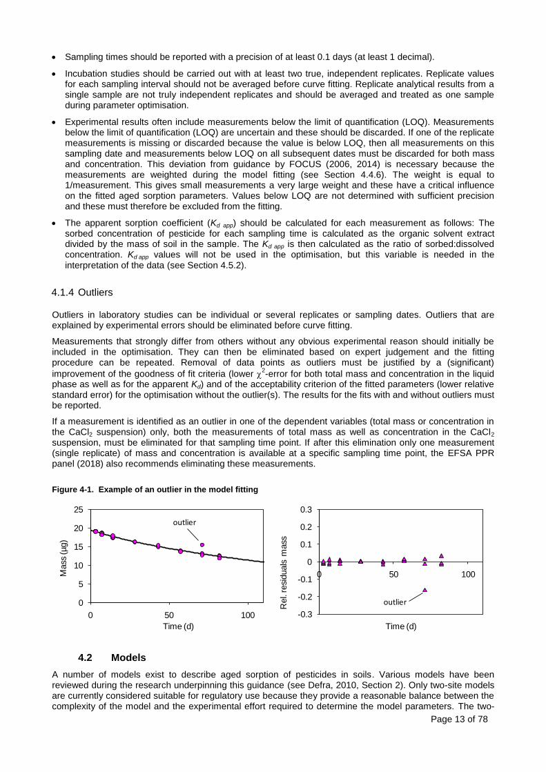
If a measurement is identified as an outlier in one of the dependent variables (total mass or concentration in the CaCl2 suspension) only, both the measurements of total mass as well as concentration in the CaCl2 suspension, must be eliminated for that sampling time point. If after this elimination only one measurement (single replicate) of mass and concentration is available at a specific sampling time point, the EFSA PPR panel (2018) also recommends eliminating these measurements.

Figure 4-1. Example of an outlier in the model fitting

4.2 Models

A number of models exist to describe aged sorption of pesticides in soils. Various models have been reviewed during the research underpinning this guidance (see Defra, 2010, Section 2). Only two-site models are currently considered suitable for regulatory use because they provide a reasonable balance between the complexity of the model and the experimental effort required to determine the model parameters. The two-

0

5

10

15

20

25

0 50 100

Mass

(µg)

Time (d)

-0.3

-0.2

-0.1

0

0.1

0.2

0.3

0 50 100

Rel. resi

duals

mass

Time (d)

outlier

outlier

Page 14 of 78

site model was demonstrated to give a good description of the measured increase in sorption for a large number of datasets (Hardy, 2011). In the exceptional cases that sorption cannot be described by the two-site model, this leads to an unacceptable model fit that is then excluded from further use.

More complex models (e.g. diffusion models) include more microscopic mechanistic detail than necessary to describe the phenomena observed at the macroscopic level and do not necessarily improve the fit to the experimental data, and robust parameters are more difficult to derive. Simpler models (empirical equations, one-site models) do not have the flexibility to describe the experimental observations under a wide range of conditions, ignore important dependencies between processes, coupling with leaching models or use for simulations of repeated pesticide applications is difficult. Two-site models are now implemented into the software packages FOCUS PEARL, MACRO 5.0 onwards, FOCUS PELMO and FOCUS PRZM to enable the simulation of kinetic sorption (EC, 2014a).

FOCUS PEARL

The leaching model FOCUS PEARL uses the two-site model according to Leistra et al. (2001). The same two-site model is implemented for a laboratory system in the PEARLNEQ software. This software can be used to derive input parameters for FOCUS PEARL. The PEARLNEQ model is depicted in Figure 4-2.

Figure 4-2. Schematic representation of the PEARLNEQ model showing the soil solution on the right and the equilibrium and non-equilibrium sorption sites on the left. Only pesticide in the equilibrium domain (indicated by the dashed line) is subject to degradation.

The two-site model assumes that sorption is instantaneous on one fraction of the sorption sites and slow on the remaining fraction (Leistra et al., 2001). The term ‘sites’ is used loosely here, not necessarily referring to molecular binding sites: For describing pesticide partitioning into organic matter, one may prefer to use the terms ‘equilibrium domain’ and ‘non-equilibrium domain’, or ‘fast-sorption domain’ and ‘slow-sorption domain’.

Sorption in both domains is described by a Freundlich equation, but sorption in the equilibrium domain of the model is instantaneous, and sorption in the non-equilibrium domain is rate-limited.

Degradation is described by first-order kinetics. Only molecules present in the equilibrium domain (the liquid phase and sorbed in the equilibrium domain) are assumed to degrade. Molecules sorbed in the non-equilibrium domain are considered not to degrade.

The PEARLNEQ model can be described as follows:

𝑀𝑝 = 𝑉𝑐𝐿 + 𝑀𝑆(𝑋𝐸𝑄 + 𝑋𝑁𝐸) (1)

𝑋𝐸𝑄 = 𝐾𝐹,𝐸𝑄 𝑐𝐿,𝑅 (𝑐𝐿

𝑐𝐿,𝑅)

1/𝑛

(2)

𝑑𝑋𝑁𝐸

𝑑𝑡= 𝑘𝑑𝑒𝑠 (𝐾𝐹,𝑁𝐸 𝑐𝐿,𝑅 (

𝑐𝐿

𝑐𝐿,𝑅)

1/𝑛

− 𝑋𝑁𝐸) (3)

equilibrium

sorption

non-equilibrium

sorptionFreundlich

KF,NE 1/n

fNE = Ratio KF,NE:KF,EQ

Freundlich

KF,EQ 1/n

Desorption Rate Constant

kdes

Transformation

kt

Page 15 of 78

𝐾𝐹,𝑁𝐸 = 𝑓𝑁𝐸𝐾𝐹,𝐸𝑄 (4)

𝑑𝑀𝑝

𝑑𝑡= −𝑘𝑡(𝑉𝑐𝐿 + 𝑀𝑆𝑋𝐸𝑄) (5)

𝐾𝐹,𝐸𝑄 = 𝑚𝑂𝑀𝐾𝑂𝑀,𝐸𝑄 (6)

where:

Mp = total mass of pesticide in each jar (g), acronym Mas V = the volume of water in the soil incubated in each jar (mL), acronym VolLiq Ms = the mass of dry soil incubated in each jar (g), acronym MasSol

cL = concentration in the liquid phase (g/mL), acronym ConLiq

cL,R = reference concentration in the liquid phase (g/mL), acronym ConLiqRef

XEQ = content sorbed at equilibrium sites (g/g)

XNE = content sorbed at non-equilibrium sites (g/g) KF,EQ = equilibrium Freundlich sorption coefficient (mL/g), acronym CofFreEql KF,NE = non-equilibrium Freundlich sorption coefficient (mL/g), acronym CofFreNeq 1/n = Freundlich exponent (-), acronym ExpFre kdes = desorption rate coefficient (d

-1), acronym CofRatDes

fNE = ratio between equilibrium and non-equilibrium Freundlich coefficients (-), acronym FacSorNeqEql kt = degradation rate coefficient (d

-1)

mOM = mass fraction of organic matter in the soil (kg/kg), acronym CntOm KOM,EQ = coefficient of equilibrium sorption on organic matter (mL/g), acronym KomEql

The model has six parameters: the initial concentration of the pesticide, the degradation rate constant kt, the equilibrium sorption coefficient KOM,EQ, the Freundlich exponent 1/n, the ratio of non-equilibrium sorption to equilibrium sorption fNE and the (de)sorption rate constant kdes.

The rate of partitioning into the non-equilibrium domain is represented by the rate constant kdes (d-1

). The term ‘desorption rate constant’ is somewhat misleading, as the rate constant is used for both adsorption and desorption in the slow sorption domain: Adsorption will be the dominating process just after application of the pesticide, but due to degradation in the equilibrium domain, the process reverses at some point in time, which initiates desorption from the non-equilibrium domain back into the equilibrium domain. Both directions are described by the same rate constant kdes. The slow transfer described by the rate constant kdes could be mediated by a number of microscopic processes (e.g. diffusion, slow chemical reactions). For modelling the slow transfer, it is however not necessary to specify the underlying process.

The model does not explicitly account for irreversible sorption. Non-extractable residues are considered irreversibly sorbed or degraded and excluded from the residue data in the model fitting. This approach is consistent with the FOCUS approach for deriving DegT50 values (FOCUS, 2014).

It is worth pointing out that the model describes Freundlich sorption. This means that the model can distinguish between the increase in sorption over time due to aged sorption (enhanced binding to the soil), and the shift towards the sorbed state that is caused by sorption non-linearity for Freundlich exponents < 1 (the relative proportion of sorbed pesticide increases over time when the total mass declines because the relationship between sorbed and dissolved pesticide is non-linear). MACRO A very similar model has been implemented into the pesticide leaching model MACRO (Larsbo and Jarvis, 2003). It is based on the model by Streck et al. (1995). The rate equation used by PEARLNEQ (Equation 3) differs from that used by MACRO:

𝑑𝑋𝑁𝐸

𝑑𝑡=

𝛼𝑀𝐴𝐶𝑅𝑂

𝑓𝑁𝐸 𝑀𝐴𝐶𝑅𝑂(𝐾𝐹,𝑇𝑜𝑡𝑎𝑙𝑐𝐿,𝑅 (

𝑐𝐿

𝑐𝐿,𝑅)

1/𝑛

− 𝑋𝑁𝐸) (7)

The definition of fNE is also different in MACRO. Here, fNE expresses non-equilibrium sorption as a fraction of total sorption (Equation 8) whereas fNE in PEARLNEQ is the ratio of non-equilibrium to equilibrium sorption (Equation 4).

Page 16 of 78

𝑓𝑁𝐸 𝑀𝐴𝐶𝑅𝑂 =𝐾𝐹,𝑁𝐸

𝐾𝐹,𝐸𝑄 + 𝐾𝐹,𝑁𝐸 (8)

where:

XNE = content sorbed at non-equilibrium sites (g/g) αMACRO = desorption rate coefficient (d

-1) used in MACRO.

fNE MACRO = fraction of the non-equilibrium sorption sites in MACRO (-) KF,Total = sum of equilibrium plus non-equilibrium Freundlich sorption coefficient (mL/g) KF,EQ = equilibrium Freundlich sorption coefficient (mL/g) KF,NE = non-equilibrium Freundlich sorption coefficient (mL/g)

The degradation rate on the non-equilibrium sites in MACRO can be set equal to the rate in the equilibrium domain, or to zero. Zero degradation in the non-equilibrium domain is identical to the concepts in PEARLNEQ. The relationship between the parameters used in MACRO and PEARLNEQ (EC, 2014a) is:

𝑓𝑁𝐸 𝑀𝐴𝐶𝑅𝑂 =𝑓𝑁𝐸 𝑃𝐸𝐴𝑅𝐿

1 + 𝑓𝑁𝐸 𝑃𝐸𝐴𝑅𝐿 (9)

𝑓𝑁𝐸 𝑃𝐸𝐴𝑅𝐿 =𝑓𝑁𝐸 𝑀𝐴𝐶𝑅𝑂

1 − 𝑓𝑁𝐸 𝑀𝐴𝐶𝑅𝑂 (10)

𝛼𝑀𝐴𝐶𝑅𝑂 = 𝑘𝑑𝑒𝑠 𝑃𝐸𝐴𝑅𝐿

𝑓𝑁𝐸 𝑃𝐸𝐴𝑅𝐿

1 + 𝑓𝑁𝐸 𝑃𝐸𝐴𝑅𝐿 (11)

𝑘𝑑𝑒𝑠 𝑃𝐸𝐴𝑅𝐿 =𝛼𝑀𝐴𝐶𝑅𝑂

𝑓𝑁𝐸 𝑀𝐴𝐶𝑅𝑂 (12)

PELMO and PRZM The current versions of the FOCUS models FOCUS-PELMO 5.5.3 and FOCUS PRZM 4.6.2 use the same aged sorption model as FOCUS PEARL. The parameters derived with the PEARLNEQ model can be entered directly into PELMO or PRZM.

4.3 Tools

Several tools are available for fitting the two-site model to the data. The model parameters are derived by an optimisation procedure. The estimation of parameter values from aged sorption studies consists of several steps:

1. Entering the measured data for each sampling time.

2. Making an initial guess for each parameter value of the selected model (referred to as “starting value”).

3. Calculation of the data at each time point.

4. Comparison between the calculated and measured data.

5. Adjustment of the parameter values until the discrepancy between the calculated and measured concentrations is minimised (“best fit”).

Steps 3-5 are carried out automatically within software tools. These packages start from the initial guess made by the modeller and repeatedly change the parameter values in order to find the best-fit combination. In order to use such an automated procedure, “best fit” must be defined in the form of a mathematical expression referred to as the ‘objective function’. Often, the sum of the squared differences between the calculated and observed data (sum of squared residuals = SSQ) is used. The software package aims at finding the combination of parameters that gives the smallest SSQ. This method is referred to as least squares method. Maximum likelihood methods can also be used. These maximise the probability that the simulated curve is an exact match of the measured data. The method to adjust the parameter values from the previous guess based on the objective function differs between different tools. Many optimisation packages use the Levenberg-Marquardt algorithm. This method

Page 17 of 78

linearises the differential model equations and calculates the model output for the initial parameter guess based on the linear equation. It then changes the parameters one at a time up or down (or in both directions), calculates the model output again and compares the objective function between the old and new parameter value(s). The change in the objective function drives the size and direction of the next change in the parameter value. When the objective function no longer changes, the parameter value at that point is returned as the optimum value. The standard error of the parameter is calculated as a function of i) the value of the objective function at the optimum, ii) the total number of observations, iii) the number of parameters and iv) the linearised form of the differential equations. The confidence interval is calculated from the standard error based on the assumption that the standard errors are normally distributed. An alternative approach is the Markov Chain Monte Carlo method (Görlitz et al., 2011). The Levenberg-Marquardt algorithm varies parameters within the constraints specified by the user and gives equal probability to all values between these boundaries. In contrast, the expected type and width of the parameter distribution can be specified in the Markov Chain Monte Carlo method. For example, it may be expected that the parameter DegT50EQ lies somewhere within a log-normal distribution with a mean of 20 days and a standard deviation of 5. This gives values near 20 a higher probability than values at the tails of the distribution. A parameter value is selected from this distribution and the objective function is calculated. The parameter value is then changed and the objective function is calculated again. The parameter distribution is updated during the optimisation based on the differences between the objective functions at each step. The final distribution gives information on the most likely parameter value that gives the best fit. The confidence intervals can be derived directly from the final parameter distribution. The Levenberg-Marquardt algorithm changes the parameter value up or down from its starting point. It can get ‘trapped’ in a region where the objective function is small (’local minimum’) without realising that even smaller objective functions (‘global minimum’) could be achieved if the parameter changed to a value far away from the starting point. The Markov Chain Monte Carlo method evaluates the objective function for the whole distribution of possible parameter values. It is, thus, in principle more likely to find the global minimum of the optimisation than the Levenberg-Marquardt algorithm, provided the assumed distribution includes the true optimum parameter. However, the settings for the Levenberg-Marquardt algorithm can be fine-tuned to ensure that the global minimum is reached. An additional optimisation method that could be used is the Iteratively Reweighted Least Squares (IRLS) method described by Gao et al. (2011). IRLS is recommended when performing standard degradation kinetic assessments with parent and metabolites. Previously the use of ordinary least squares regression techniques were recommended for such kinetic fitting. These assume that the error variance is the same for parent and metabolite and produces an unweighted fit. Ordinary least squares can significantly overestimate the confidence interval for the metabolite because the error variance for parent can be significantly larger than for the metabolite, especially when concentrations of a metabolite are significantly smaller than for the parent. In these cases, weighted fits, using IRLS for example, have advantages. Considering the aged sorption model, concentrations in the equilibrium domain can also be significantly smaller than the total mass, and hence the error variance can also be significantly smaller. Hence the use of IRLS is also recommended in these cases. Three tools that are commonly used to derive aged sorption parameters are briefly described below. Alternative optimisation packages can be used provided the tool and optimisation settings give robust fits. The independence of the optimised parameter values from the starting values must be demonstrated because this increases the likelihood that the global minimum can be reached. The optimisation package must also provide the output that is required to assess the goodness of fit according to Section 4.5 (e.g. confidence interval or standard error). Ideally, the results from the alternative tool should be compared with those from one of the three tools described below. This is intended to be a one-off test of the alternative optimisation package, a comparison with other tools is not required after the similarity of results has been demonstrated for example datasets. The EFSA PPR panel (2015) does not recommend a specific software tool. Requirements are that the tool and optimisation settings provide a robust fit, and that it provides the required output to assess the goodness of fit as described in this guidance. The minimum requirements are listed below:

• Capabilities

– It should be able to calculate all parameters of the aged sorption model.

– It should be able to deliver all statistics that are used to assess the goodness of fit.

– It should provide graphical information of the fits and the residuals.

Page 18 of 78

• Documentation

– A description of the implementation of the aged sorption concept in the software must be available.

– A user manual, i.e. a detailed description on how the tool is operated, must be available. This should include a description of model inputs and model outputs.

– A description of all statistics or a reference to documentation in which the statistical methods are fully described must be available.

– A description that the tool works correctly (e.g. by testing against a benchmark data set) should be provided.

• Compatibility

– The tools should be available for major operating systems (like Windows 7–10).

• Availability

– Easily obtainable, for example downloadable from a website.

– Support from the developer or distributor of the software.

– Earlier versions, if applicable, should be available upon request.

– Preferably the tool is available free of charge.

• User interface

– To facilitate use of the tool by regulators, the software tool should be accessible via a graphical user interface. The general setup of the user interface should be discussed with regulators and developers of the tool.

– Functionality to run the tool in batch mode would be a helpful addition.

4.3.1 PEARLNEQ

PEARLNEQ combines the two-site model that is implemented in FOCUS PEARL with the optimisation software PEST (Doherty, 2005). The model is simultaneously fitted against data on the total mass of the pesticide in soil (µg) and the concentration in the liquid phase (µg/mL). PEARLNEQ is run repeatedly by PEST and the parameters are adjusted until the best possible fit to the measured data is achieved based on the least squares method and the Gauss-Marquardt-Levenberg algorithm. The program is DOS based and operates on command file or command line level. Boesten et al. (2007) provide a short description of PEARLNEQ. The program package of PEARLNEQ includes the PEARLMK.EXE program that produces all necessary PEST files with the help of a text file with the extension .mkn. In order to carry out the non-equilibrium parameter estimation procedure in PEARLNEQ, the *.mkn file of the PEARLNEQ package has to be compiled following the instructions in the PEARLNEQ manual. The *.mkn file of PEARLNEQ for an example case is given in Appendix 2. The output generated by PEST includes the fitted parameters and their 95% confidence intervals, the sum of squared residuals and daily output of the calculated total mass and liquid phase concentration for a period specified by the user. PEARLNEQ v5 offers an option to perform temperature normalisation. However, the EFSA PPR panel (2018) argued that this procedure is prone to error and therefore it is now recommended to perform the normalisation of DegT50EQ to the reference temperature outside PEARLNEQ. In PEARLNEQ this is achieved by setting the reference temperature to the incubation temperature.

4.3.2 ModelMaker 4.0

ModelMakerTM

is one of the tools that are recommended for parameter fitting within the framework of FOCUS kinetics (a more detailed description can be found in FOCUS, 2006, 2014). It allows users to build their own models using inter-linked variables or compartments. Gurney and Hayes (2007) describe an implementation of the two-site model by Leistra et al. (2001) into ModelMaker

TM (Figure 4-3). ModelMaker

TM allows the user

Page 19 of 78

to optimise the equilibrium sorption coefficient KOM,EQ. Several replicates can be fitted simultaneously. The best possible fit to the measured data is achieved based on the Levenberg-Marquardt algorithm. ModelMaker

TM provides output of the optimised parameter values and their standard error, a graphical plot of

the measured and calculated data and the calculated values in tabulated form. Figure 4-3. Implementation of non-equilibrium sorption in ModelMaker

TM

4.3.3 MatLab

MatLabTM

(2007) is a numerical computing environment and fourth generation programming language. Developed by The MathWorks®, MatLab

TM allows matrix manipulation, plotting of functions and data,

implementation of algorithms, creation of user interfaces, and interfacing with programs in other languages. MatLab

TM can be applied to build and solve mathematical models such as the two-site model. Add-on

toolboxes are available for solving differential equations and to solve the optimisation of model parameters. The MatLab

TM code can be tailored to the user’s requirements.

BayerCrop Science integrated the two-site model into an Excel® spreadsheet that calls MatLab

TM via Excel

Link™. The parameters are adjusted based on the least squares method and the Marquardt-Levenberg algorithm. This is an option within the MatLab

TM routine lsqnonlin (Solve nonlinear least-squares data-fitting

problems). The default optimisation settings are used. The Markov Chain Monte Carlo method or Iteratively Reweighted Least Squares method could be implemented instead of the Marquardt-Levenberg algorithm. Further modifications could be made to bring the version in line with the guidance outlined in this document (e.g. fitting of KOM,EQ, additional graphical outputs). The tool generates various statistical outputs. The FOCUS Groundwater II group fitted the two-site model to the total mass and liquid phase concentration for an example dataset using the three software tools PEARLNEQ, ModelMaker

TM and MatLab

TM. The

results for all three tools were almost identical (EC, 2014a).

4.4 Optimisation procedure

This guidance below refers to the optimisation of the aged sorption model by Leistra et al. (2001). The procedures for the optimisation of the two-site model by Streck et al. (1995) are very similar.

4.4.1 Variables used in the optimisation.

The two-site model comprises several variables (total mass, mass sorbed in equilibrium domain, mass sorbed in non-equilibrium domain, concentration in liquid phase). The model should ideally be fitted to the data on total mass and concentrations in the liquid phase because these are directly measured during the experiment. An alternative procedure was tested by the FOCUS GW II group (EC, 2014a). MatLab was used to fit the two-site model to the sorbed mass in the equilibrium and non-equilibrium domains. These variables

Page 20 of 78

were calculated from the measured organic solvent and aqueous extractable residues. The parameters derived with this method were compared with those optimised against the total mass and concentrations in the liquid phase. The FOCUS GW II group found that the parameter values were independent of the variables fitted, but the standard deviation of the parameters was smaller for the fits to sorbed mass. However, additional modelling showed that the two methods are equivalent. In radiolabelled studies, the radioactivity measured in the aqueous and solvent extracts must be characterised and converted to mass and concentrations of the parent compound of interest.

4.4.2 Fitted parameters

Aged sorption model The two-site model described by Leistra et al. (2001) has six parameters (Mp ini, KOM,EQ,1/n, kt, kdes and fNE), see Section 4.2. All parameters except 1/n should be optimised against measured data. In the optimisation tool PEARLNEQ, the parameter kt is not optimised directly. The degradation half-life (DegT50EQ, days) is optimised instead, and kt is calculated within the model as ln(2)/ DegT50EQ. In theory, the Freundlich exponent 1/n could be derived in aged sorption studies, if each aged sorption study was carried out with a range of initial pesticide concentrations. However it would not be practical to carry out such a large number of experiments. Therefore the 1/n value in the aged sorption model should be fixed to the 1/n value that was determined in a batch sorption study on the same soil. Equilibrium sorption model A model fit should also be undertaken with equilibrium sorption only. The non-equilibrium component of the model can be switched off by fixing fNE and kdes to zero. PEARLNEQ gives the option to select the equilibrium model in the input file. Only Mp ini, DegT50EQ and KOM,EQ are then optimised against the weighted data for mass and liquid phase concentration. The results of this optimisation are used as a benchmark for comparison with the fit by the two-site model.

4.4.3 Optimisation settings

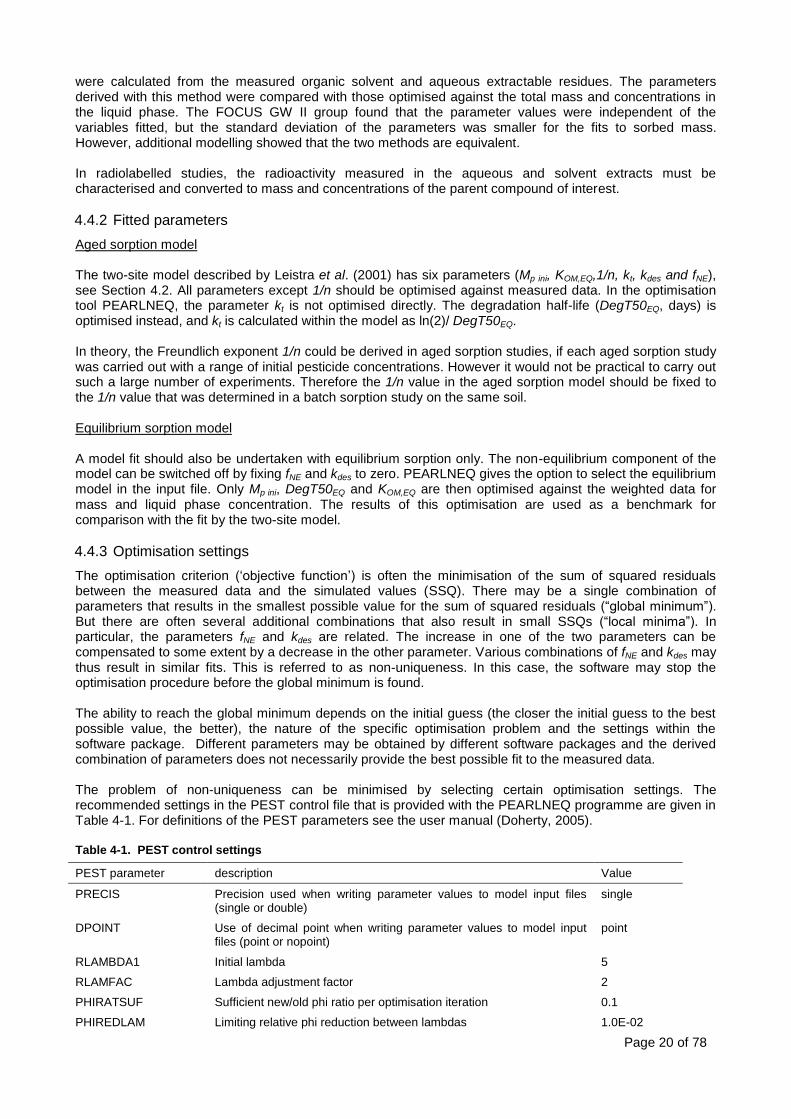
The optimisation criterion (‘objective function’) is often the minimisation of the sum of squared residuals between the measured data and the simulated values (SSQ). There may be a single combination of parameters that results in the smallest possible value for the sum of squared residuals (“global minimum”). But there are often several additional combinations that also result in small SSQs (“local minima”). In particular, the parameters fNE and kdes are related. The increase in one of the two parameters can be compensated to some extent by a decrease in the other parameter. Various combinations of fNE and kdes may thus result in similar fits. This is referred to as non-uniqueness. In this case, the software may stop the optimisation procedure before the global minimum is found. The ability to reach the global minimum depends on the initial guess (the closer the initial guess to the best possible value, the better), the nature of the specific optimisation problem and the settings within the software package. Different parameters may be obtained by different software packages and the derived combination of parameters does not necessarily provide the best possible fit to the measured data. The problem of non-uniqueness can be minimised by selecting certain optimisation settings. The recommended settings in the PEST control file that is provided with the PEARLNEQ programme are given in Table 4-1. For definitions of the PEST parameters see the user manual (Doherty, 2005). Table 4-1. PEST control settings

PEST parameter description Value

PRECIS Precision used when writing parameter values to model input files (single or double)

single

DPOINT Use of decimal point when writing parameter values to model input files (point or nopoint)

point

RLAMBDA1 Initial lambda 5

RLAMFAC Lambda adjustment factor 2

PHIRATSUF Sufficient new/old phi ratio per optimisation iteration 0.1

PHIREDLAM Limiting relative phi reduction between lambdas 1.0E-02

Page 21 of 78

PEST parameter description Value

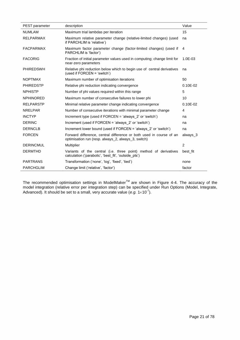
NUMLAM Maximum trial lambdas per iteration 15

RELPARMAX Maximum relative parameter change (relative-limited changes) (used if PARCHLIM is ‘relative’)

na

FACPARMAX Maximum factor parameter change (factor-limited changes) (used if PARCHLIM is ‘factor’)

4

FACORIG Fraction of initial parameter values used in computing; change limit for near-zero parameters

1.0E-03

PHIREDSWH Relative phi reduction below which to begin use of central derivatives (used if FORCEN = ‘switch’)

na

NOPTMAX Maximum number of optimisation iterations 50

PHIREDSTP Relative phi reduction indicating convergence 0.10E-02

NPHISTP Number of phi values required within this range 5

NPHINORED Maximum number of consecutive failures to lower phi 10

RELPARSTP Minimal relative parameter change indicating convergence 0.10E-02

NRELPAR Number of consecutive iterations with minimal parameter change 4

INCTYP Increment type (used if FORCEN = ‘always_2’ or ‘switch’) na

DERINC Increment (used if FORCEN = ‘always_2’ or ‘switch’) na

DERNCLB Increment lower bound (used if FORCEN = ‘always_2’ or ‘switch’) na

FORCEN Forward difference, central difference or both used in course of an optimisation run (resp. always_2, always_3, switch)

always_3

DERINCMUL Multiplier 2

DERMTHD Variants of the central (i.e. three point) method of derivatives calculation (‘parabolic’, ‘best_fit’, ‘outside_pts’)

best_fit

PARTRANS Transformation (‘none’, ‘log’, ‘fixed’, ‘tied’) none

PARCHGLIM Change limit (‘relative’, ‘factor’) factor

The recommended optimisation settings in ModelMaker

TM are shown in Figure 4-4. The accuracy of the

model integration (relative error per integration step) can be specified under Run Options (Model, Integrate,

Advanced). It should be set to a small, very accurate value (e.g. 110-7

).

Page 22 of 78

Figure 4-4. Recommended optimisation settings in ModelMaker TM

For other software tools please refer to the respective user manual.

4.4.4 Starting values

Different optimised values can be returned by the software for different combinations of initial guesses for the parameters provided by the modeller (starting values). The optimisation settings specified above for PEST and ModelMaker

TM will reduce the dependency on starting values, but the problem of non-uniqueness

cannot be fully overcome. The optimisation should thus be repeated with a number of different initial combinations of parameter values. The results of all fits should be reported and the parameter combination that gives the best objective function (e.g. the smallest SSQ) should be selected. If several starting values give identical objective functions, then the combination with the smallest relative confidence intervals (confidence interval as a fraction of the mean estimate) for fNE and kdes should be chosen. The following specific recommendations can be made:

The initial mass Mp ini, is often close to the measured concentration at the first sampling point and this can be used as a starting value in the optimisations where appropriate. An alternative is to use the added mass. The starting value for the initial mass can also be derived by fitting a first-order dissipation model to the data in a separate model run with any appropriate tool.

The initial value for the degradation half-life DegT50EQ should be set to the first-order DegT50 value. This can be derived by fitting a first-order model to the total parent mass data in a separate model run with any appropriate tool.

The initial value for KOM,EQ should be set to the value obtained in the batch sorption experiments (OECD 106).

At least four different initial guesses should be tested for fNE and kdes (Table 4-2). The same starting value for Mp ini, DegT50EQ and KOM,EQ should be used in all optimisations.

Table 4-2. Starting values for fNE and kdes

fNE kdes

0.2 0.004 0.2 0.05 1.5 0.004 1.5 0.05

Page 23 of 78

4.4.5 Parameter ranges

For some parameters, it may be useful to define ranges within which the parameter will be varied during optimisation. This will prevent convergence at unrealistic local minima. A lower boundary > 0 will avoid numerical problems during the optimisation (division by zero). The recommended constraint range for fNE during optimisation is from 0.001 to 50, and the recommended constraint range for kdes is from 0.00001 to 0.5 d

-1. These boundaries can be adjusted if needed, but within the limits of the model used for calculation of

PEC in groundwater. The maximum value for kdes that can be entered in PEARL and PEARLNEQ is 0.5 d-1

. Boundaries for Mp ini, DegT50EQ and KOM,EQ may also need to be set and reported.

4.4.6 Weighting

Aged sorption models should be simultaneously fitted to measurements for the total mass of a pesticide in soil and the concentration in the liquid phase. The absolute values for the mass are often much larger than the concentrations depending on the strength of sorption and the unit used (e.g. µg for the total residue and µg/mL for the aqueous concentration). The same relative deviation of the modelled data from the calculated values results in much greater squared residuals when the absolute value of the measurement is large. As a result, an unweighted model fit will usually be dominated by the total mass and only marginally influenced by the liquid phase concentrations. This can lead to a good fit to the mass, but a poor fit to the concentrations. This can also result in large confidence intervals for the parameters kdes and fNE. The measurements must be weighted during the optimisation to minimise this problem. Weighted fitting applies a correction factor to the residuals:

Φ = ∑(𝑤𝑖𝑟𝑖)2

𝑚

𝑖=1

(13)

where is the object function, ri is the residual (difference between the simulated and the measured value corresponding to measurement i ), wi is the weighting factor and m is the total number of measurements (sum of number of measurements of Mp and cL). The preferred option is to define wi as the inverse of the measured value of Mp or cL. This will reduce the weight of the mass data and increase the weight of the concentration data compared with unweighted fitting.

Φ = ∑ (∆𝑀𝑝,𝑖

𝑀𝑝,𝑖)

2𝑛

𝑖=1

+ ∑ (∆𝑐𝐿,𝑗

𝑐𝐿,𝑗)

2𝑜

𝑗=1

(14)

where n is the number of measurements for the mass and o is the number of measurements for the concentration in the liquid phase (note that n=o), ΔMp,i is the difference between the simulated and observed mass for measurement i , Mp,i is the observed mass for measurement i, ΔcL,j is the difference between the simulated and observed concentration in the liquid phase for measurement j, and cL,i is the observed concentration in the liquid phase for measurement j. The time series of mass data consists of larger values at the beginning of the experiment and smaller values at the end. The same is true for the time series of concentration data. Weighting by the reciprocal value implies that the relative error in the measurements is constant with time, i.e. larger values for mass and concentration are measured with the same relative accuracy than small values. This assumption was supported by an analysis of measured data by Defra (2010). Weighting by 1/measurement (equation 14) is one of the options implemented in PEARLNEQ. The optimisation settings in ModelMaker

TM should be set to those shown in Figure 4-5 to match those in

PEARLNEQ (click on Advanced to access the weighting options).

Page 24 of 78

Figure 4-5. Recommended settings for data weighting in ModelMakerTM

– Option 1

Alternatively, the weights can be entered in the model data table as an additional column (Figure 4-6). ModelMaker

TM divides the residuals by the weight specified by the user. The weights must thus be identical

to the measurements (and not the inverse value). Figure 4-6. Recommended settings for data weighting in ModelMaker

TM – Option 2

4.5 Goodness of fit criteria

The decision on whether a model fit is acceptable or not should be based on:

An assessment of the visual fit of the mass and liquid phase concentration and of the apparent Kd values plotted against time;

An assessment of the weighted residuals of the mass and liquid phase concentration and of the apparent Kd values plotted against time;

A 2-test to assess the goodness of fit of the model to the data for mass and concentration;

No individual measurement of goodness of fit can be recommended as being more important than the others and an analysis of all criteria listed above should always be performed. The goodness of fit criteria should

Page 25 of 78

always be fully reported and described in order to allow independent validation of the fitting procedure. An example assessment of the goodness of fit is presented in Appendix 2.

4.5.1 Visual assessment of model fit

Measured and fitted data must always be presented graphically and a visual assessment of the goodness of fit must be made (only the results for the starting values of fNE and kdes that give the best fit need to be plotted): 1. Measured mass and aqueous concentration data and the calculated curves should be plotted versus

time. 2. Apparent linear Kd values (Kd,app) should be calculated from the measured data and the simulated

concentrations and plotted against time. Apparent Kd values at each time point are calculated as follows:

𝑋(𝑡) =𝑀𝑝(𝑡)

𝑀𝑆−

𝑉𝑡𝑜𝑡

𝑀𝑆𝑐𝐿(𝑡) (15)

𝐾𝑑 𝑎𝑝𝑝(𝑡) =𝑋(𝑡)

𝑐𝐿(𝑡) (16)

where:

X (t) = content sorbed at time t (g/g)

Mp (t) = total mass of pesticide in each jar at time t (g) Ms = the mass of dry soil incubated in each jar (g) Vtot = the volume of water in the sample during CaCl2 extraction (mL)

cL (t) = concentration in the liquid phase at time t (g/mL) Kd app (t) = apparent Kd value at time t (mL/g) Apparent Kd values are usually more scattered than the data on mass and concentration. It is important that the apparent Kd value shows an increase over time that can be distinguished from the scatter in the data. Figure 4-7 gives an example of an acceptable and unacceptable pattern of Kd app. Figure 4-7. Example of acceptable (left) and unacceptable (right) patterns of apparent Kd values

It is also important to compare the modelled line with the experimental apparent Kd values. Sometimes, mass and liquid phase concentrations are described well by the model, but the apparent Kd is not. In this case, the fit should be rejected. An example of an acceptable and unacceptable description of Kd app is given in Figure 4-8. The unacceptable fit on the right-hand side of Figure 4-8 illustrates that the goodness of fit cannot be assessed visually based on the mass and liquid phase concentrations alone.

0

5

10

15

20

25

30

35

0 20 40 60 80

Kd a

pp (

L/k

g)

Time (d)

0

2

4

6

8

10

12

14

16

0 20 40 60 80 100 120

Kd a

pp (

L/k

g)

Time (d)

Page 26 of 78

Figure 4-8. Illustrative example of acceptable (left) and unacceptable (right) description of the apparent Kd values by the aged sorption model

In addition to the apparent Kd values, the simulated mass sorbed in the equilibrium and non-equilibrium domain should be plotted against time. A robust fit is more likely when the mass in the non-equilibrium domain shows a phase of decline during the experimental period. Fits are also more robust when non-equilibrium sorption is an important component of the whole system (i.e. the mass in the non-equilibrium domain must not be negligible compared to the mass in the equilibrium domain). Examples are given in Appendix 2. For the use of aged sorption in groundwater leaching assessments, it is important that the model describes the long-term dynamics (weeks, months). Therefore, care should be taken that the model gives a good description of the overall long-term increase in sorption. The EFSA PPR panel (2018) does not recommend refinement options for the optimisation compared with the procedure outlined in the Sections above. This is because this may require expert judgement and lead to additional discussions in the absence of clear recommendations on when to consider a refined fit superior to the standard fit.

4.5.2 Visual assessment of weighted residuals

Residual plots should be used to assist in the visual assessment of the goodness of fit. The fitting of the model to the data was performed based on weighted residuals, see Section 4.4.6. Therefore, weighted residuals should be used for the residual plots. Each residual is weighted with the reciprocal value of the measurement. These are calculated as: (simulated value – measured value) / measured value. Weighted residuals for the mass, liquid phase concentration and Kd,app data should be plotted vs. time to assess the visual fit of the model to the data.

Page 27 of 78

An assessment of the residuals is useful for revealing patterns of over- or under-predictions. For an exact fit, all residuals are zero. Systematic deviations become apparent when negative and positive residuals are not randomly scattered around the zero line (for example, 3 or more consecutive positive or negative residuals may indicate a systematic deviation). Absolute residuals have the same unit as the measurement, whereas weighted residuals are simply fractions of the measurements. For example, a weighted residual of 0.2 means that the simulated value exceeds the measured value by 20%. This facilitates the assessment across the 3 types of data (mass, liquid phase concentration and Kd,app) and makes the interpretation more intuitive. The drawback of weighted residuals is that deviations between small values are magnified. The precision of small measured mass and concentration data is therefore very important. As stated previously, data with less than 3 significant figures must not be included in the assessment. Please note that using the best combination of parameters does not guarantee a good fit to the measured data. If the model is not appropriate to describe measured behaviour, even the best possible parameter combination for that model will not give an adequate fit to the data. The model will not be able to describe the data, for example, if degradation is biphasic for reasons other than aged sorption, or if degradation shows a lag-phase. Always evaluate the visual fit to decide if a model is acceptable. In contrast to first-tier degradation studies, where alternative models such as double first-order in parallel (DFOP), first-order multi-compartment (FOMC) or first-order sequential biphasic (hockey stick) models can be used if the single first-order (SFO) model fails to describe the observed behaviour (trend in the residues), these options are not available for aged sorption. Due to a lack of alternative model descriptions for degradation (biphasic models) and sorption complexity (multiple sorption sites), the EFSA PPR panel (2018) recommends that only a trend in the weighted residuals of both total mass and concentration in the CaCl2 suspension invalidates the aged sorption model used. The soil should then be classified as having ‘zero aged sorption’.

4.5.3 Chi2-test for assessing the goodness of fit

FOCUS (2006, 2014) proposed a 2-test to evaluate the goodness of fit of degradation kinetics. As the aged

sorption model is fitted to weighted data, a modified version of the test should be applied:

𝜒2 = ∑(𝑃𝑖 − 𝑂𝑖)

2

(𝜒2𝑒𝑟𝑟𝑜𝑟/100 × 𝑂𝑖)2

𝑡

𝑖=1

(17)

The calculated 2 for a specific fit may be compared to tabulated

2f,

where t = number of time points for mass plus number of time points for concentration Pi = predicted value for measurement i Oi = observed value for measurement i (replicates must be averaged to give a single value for

each time point)

2-error = measurement error percentage

f = degrees of freedom = t minus number of fitted model parameters

= probability that one may obtain the given or higher 2 by chance.

Data for mass and concentration are included in the calculation of the 2-error. Note that replicates should be

averaged to give a single value for mass, and a single value for concentration for each time point. Data that

were not included in the data fitting are not included in the test. The 2-test considers the deviations between

observed and predicted values relative to the uncertainty of the measurements. Ideally, the measurement of uncertainty at each time point should be determined from numerous replicate values. Such replicate values are rarely available. Therefore, a pragmatic approach to define the measurement variation was proposed by FOCUS (2006, 2014). The error of the measurements was simply defined as a percentage of the average of all measurements. This implies that the absolute error is identical for all measurements (i.e. for all time points). This is consistent with the recommendation of unweighted fitting by FOCUS (2006, 2014). In contrast, the guidance on aged sorption studies proposes fitting to weighted data for mass and liquid phase concentrations. Therefore, the definition of the error has been changed to reflect the assumptions that underlie weighted fitting. The error is now defined as a percentage of each individual measurement (see denominator in Equation 17). As a result, the relative error is the same for all measurements (i.e. all concentrations can be measured with the same relative precision). The absolute error is now larger for large measurements.

Page 28 of 78

The 2-test can be used to test the agreement between calculated and observed for a given fit. A suitable

model should pass the test at a significance level of 5%. However, this assessment is only possible if the percent error is known. This is often not the case. Instead, the minimum error percentage at which the test is

passed (i.e. where the calculated value of 2 is equal to or smaller than the standard tabulated value at the

5% significance level and the given degrees of freedom) can be directly derived from Equation 17.

𝑒𝑟𝑟𝑜𝑟(%) = 100% × √1

𝜒2𝑡𝑎𝑏𝑢𝑙𝑎𝑡𝑒𝑑

∑(𝑃𝑖−𝑂𝑖)2

𝑂𝑖2

𝑡

𝑖=1

(18)

2tabulated = standard tabulated value at the 5% significance level and the given degrees of freedom

The degrees of freedom for calculating 2-error for concentration and mass is calculated as twice the number

of time points minus the number of fitted parameters. Note that the number of fitted parameters depends on

the model (i.e. aged sorption or equilibrium model). The degrees of freedom for calculating 2-error for Kd is

calculated as the number of time points minus the number of fitted parameters. Table 4-3. Number of fitted parameters and degrees of freedom for aged sorption and equilibrium models

Model Number of fitted parameters Degrees of freedom

for calculating 2-error for

concentration and mass

Degrees of freedom for

calculating 2-error for Kd

Aged sorption 5 2 n - 5 n - 5 Equilibrium 3 2 n - 3 n - 3

n = number of time points with observations

FOCUS (2006, 2014) recommends calculating a 2-error value for parent compounds and for metabolites

separately although the data for both compounds are fitted in a single optimisation. This division is necessary because unweighted fitting is carried out and because the parent and metabolite data differ in

magnitude. The modified definition of the error in the 2 test for aged sorption studies allows calculating a

single 2-error value for the mass and aqueous phase concentrations.

An analysis of 59 aged sorption datasets suggested that a 2-error of 15% is suitable as a criterion for

acceptable fits to the mass and concentration data (Defra, 2012). This must not be considered as an

absolute cut-off. The visual assessment must always be taken into account. It is possible that fits with a 2-

error percentage greater than 15% will be accepted based on the visual fit and vice versa. Where all goodness of fit criteria are not clearly met, the report should describe the rationale for accepting or rejecting certain fits.

To harmonise the calculations of the 2-error of the apparent distribution coefficient Kd,app, the PPR Panel

(2018) recommends using the unweighted method for the calculations, using the same number of fitting parameters as for the accompanying fit on mass and concentration.

The 2-error for unweighted observations is defined as follows:

𝜒2𝑒𝑟𝑟𝑜𝑟(%) = 100% × √1

𝜒2𝑡𝑎𝑏𝑢𝑙𝑎𝑡𝑒𝑑

∑(𝑃𝑖−𝑂𝑖)

2

Ō2

𝑡

𝑖=1

(19)

where i is the number of time points for Kd,app, Ō is the arithmetic mean of all calculated Kd,app values and

2tabulated is the standard tabulated value at the 5% significance level and the given degrees of freedom.

4.6 Evidence for aged sorption

It is important that the experimental data show sufficient evidence that aged sorption is relevant. If this is not the case, then it is not justified to include parameters based on the experimental study in higher tier modelling assessments. The decision as to whether there is ‘sufficient evidence’ is based on a comparison

Page 29 of 78

between the aged sorption model and an equilibrium model that ignores aged sorption (Section 4.4.2). Aged sorption is not evident if both models describe the data equally well. Note that sorption non-linearity is included in both models. A difference between the model fits thus indicates that the increase in sorption is not only caused by non-linear Freundlich sorption, but also by slow transfer or aging processes. The first judgement is made based on a visual comparison of the apparent Kd (Kd,app) plots. For aged sorption to be evident, the aged sorption model should give a better visual description of the Kd,app plots against time than the equilibrium model.

Secondly, the 2 error is used to compare the model descriptions for Kd,app. The mass and concentration data

and apparent Kd values for the equilibrium model should be plotted against time, and the 2 error should be

calculated for the apparent Kd only. Note that residual plots should show the weighted residuals whereas the

2 error is calculated using unweighted residuals.

To show the relevance of aged sorption, the 2 error percentage for the apparent Kd for the aged sorption

model must be smaller than that for the equilibrium model. Note that the number of fitted parameters is the

same as for the accompanying fit on mass and concentration for the purpose of the 2 error percentage

calculation.

4.7 Criteria for the acceptability of the fitted parameters

4.7.1 Confidence intervals and relative standard error

A confidence interval is an estimate of the uncertainty in a model parameter. The underlying assumption is: if the experiment and the estimation procedure are repeated infinitely often, then the true value of the parameter lies within the confidence interval with the chosen probability. The narrower the confidence interval, the greater the precision with which the parameter can be estimated. Wide confidence intervals can be caused by correlation between parameter values, parameter insensitivity, variability in the data, or the fact that the model cannot describe the data. Optimisation tools such as ModelMaker

TM or PEST (used for optimising PearlNEQ) give the optimised

parameters values together with the standard error or 95% confidence interval for each optimised parameter. The standard error and the confidence interval should be converted into a relative standard error (RSE) as follows:

𝑅𝑆𝐸 =𝑆𝑡𝑎𝑛𝑑𝑎𝑟𝑑 𝑒𝑟𝑟𝑜𝑟

𝜐 (20)

𝑅𝑆𝐸 =95% 𝐶𝑜𝑛𝑓𝑖𝑑𝑒𝑛𝑐𝑒 𝐼𝑛𝑡𝑒𝑟𝑣𝑎𝑙

4 𝜐 (21)

where is the fitted parameter value. The confidence interval (upper limit minus lower limit) is divided by a factor 4 to calculate the estimated standard deviation (or standard error) of the parameter fit. This is because the width of the 95% confidence interval equals 4 times the standard deviation based on a normal distribution (the fitted value plus or minus 2 × the standard deviation). Wide confidence intervals imply that the parameters are very uncertain. Where 0 is included in the confidence interval, there is not enough evidence that non-equilibrium sorption is a significant process. It is difficult to set clear cut-off criteria for acceptable confidence intervals and relative standard errors. Based on an analysis by Defra (2010) and Defra (2012), it is proposed that the RSE for any of the fitted parameters should not be greater than 0.40. This implies that the width of the 95% confidence interval must not be greater than 160% (i.e. ± 80% of the parameter estimate).

4.7.2 Correlation coefficients

EFSA (2015) recommends reporting the parameter correlation coefficient matrix (as given for example by PEST). Correlation coefficients between, for example, fNE and kdes close or equal to 1 or –1 indicate a strong interaction between these two parameters. In this case, fNE and kdes cannot be adequately determined because several combinations of fNE and kdes would lead to an acceptable fit (parameter unidentifiability).

Page 30 of 78

Strong correlation between parameters will result in large parameter uncertainty and therefore contribute to large RSE values. Therefore, it was not necessary to add a criterion in this guidance as to which correlation coefficients are acceptable, as parameters with strong correlation will fail the RSE criteria. The data is requested for information only and may help to explain some datasets that show good visual fits but large RSE values.

5 Aged sorption in the tiered pesticide leaching assessment

This section addresses how the data from the aged sorption studies should be used at the higher tier of the regulatory assessment. The EFSA PPR panel (EFSA, 2015) decided that, in order to account for aged sorption in the risk assessment, at least four of the aged sorption experiments should show evidence of aged sorption according to the criteria outlined in Section 4.6 and have reliable fNE and kdes values (i.e. minimum of four soils). If a large number of soils are tested (i.e. more than seven) then the majority of the experiments carried out should show evidence of aged sorption and yield reliable parameters. Five parameters are needed for implementing aged sorption in the PEC calculations: The Freundlich parameters KOM,EQ and 1/n are derived from batch sorption studies. The ‘aged sorption’ parameters fNE and kdes, are derived from aged sorption experiments. The fitted KOM,EQ is not used in the leaching assessment according to EFSA (2018). The DegT50EQ is derived from both aged sorption experiments, and from Tier 1 DegT50 values adjusted for aged sorption. The derivation of these input parameters is described in the following sections.

5.1 Sorption and degradation endpoints from aged sorption studies

A sensitivity analysis by Defra (2010) showed that pesticide leaching models can be very sensitive for changes in aged sorption parameters. It is thus very important to use robust parameter values in regulatory exposure assessments. Figure 5-1 illustrates the decision making procedure that must be applied to each soil-specific dataset. At each step, it is checked whether or not the study fulfils the requirements. Fitted parameters can only be used in the higher tier exposure assessment if all criteria are met. Figure 5-1. Decision Tree: Derivation of aged sorption parameters from individual experimental studies

Page 31 of 78

Zero aged sorption: In case of ‘Zero aged sorption’, the fNE and kdes for this soil are set to zero. These zero values should be included when calculating the average fNE and kdes values for the substance (Section 5.3.1), otherwise the averages would be a biased towards the soils that did show aged sorption. The sorption measurements were not suitable to derive aged sorption parameters. However, as the aged sorption study is similar to a standard degradation study (OECD 307) the residue data from this experiment can still be used to derive a lower-tier DegT50. The residue data should be processed and analysed following the lower-tier procedures for deriving a DegT50, following the FOCUS guidance on degradation kinetics (FOCUS, 2014). Fitted parameters are not reliable and cannot be used in exposure assessment: When a dataset shows evidence for aged sorption (Section 4.6) but the parameters were not acceptable because the RSE value

Page 32 of 78

failed (Section 4.7), then there are two options: The applicant may set the parameter values fNE and kdes to zero. This is an overly conservative option at this stage of the decision tree, as the dataset showed significant evidence that aged sorption occurs and setting the parameters to zero would underestimate aged sorption. The alternative option is to omit the dataset from the calculation of the average fNE and kdes. This is acceptable when the applicant has enough data for fNE and kdes from the remaining datasets. The fNE and kdes values should only be omitted if there are reliable, non-zero values of fNE and kdes from at least 4 soils remaining. In either case, the residue data from the experiment should be analysed according to FOCUS (2006, 2014) or future standard accepted kinetics guidance in order to derive a lower-tier DegT50 from this experiment. As a result, the aged sorption study should result in at least 4 values of fNE and kdes (which may include zero values) for a parent compound and at least 3 values for metabolites. In addition, the study will produce DegT50 values for each soil: DegT50EQ values will be available only from model fits that passed all criteria, but lower-tier DegT50 values can be derived for all datasets, by fitting FOCUS kinetics to the residue data. DegT50EQ values and lower-tier DegT50 values must be normalised to a temperature of 20°C and moisture of pF2 prior to groundwater modelling based on the guidance by FOCUS (EC, 2014b), unless the study was undertaken at this temperature and moisture. It is assumed that the correction factors for DegT50EQ values are the same as those for first-order DegT50 values. Note that time-step normalisation (proposed for field studies in FOCUS, 2006, 2014) is not suitable for use with aged sorption. This is because time-step normalisation would wrongly adjust the sorption rate as well as the degradation rate. The EFSA PPR panel (EFSA 2018) recommends that normalisation of the DegT50EQ for temperature should not be performed in the PEARLNEQ software, normalisation to the reference temperature should be performed outside PEARLNEQ. The moisture adjustment must be done outside PEARLNEQ.

5.1.1 Alternative ways of estimating aged sorption parameters

Research by Defra (2009) and Defra (2010) demonstrated that parameters of a two-site aged sorption model can be very variable. Aged sorption parameters for the same pesticide can differ strongly between different soils. There is no clear relationship between aged sorption parameters and soil or pesticide properties. This was confirmed by an analysis by Sur et al. (2009). This is partly due to relationships between some of the model parameters. Different combinations of parameters can give a similar result. A statistical relationship between a single parameter and soil or pesticide properties is thus difficult to establish. It is thus not recommended to estimate fNE and kdes for new pesticides from soil or pesticide properties. The FOCUS work group on groundwater scenarios (EC, 2014a) recommended default values of 0.3 for fNE and 0.01 for kdes. Analysis by Defra (2012) showed that these values are in the lower range of fNE and kdes values derived for existing studies, and therefore represent a conservative estimate, when supported by evidence that aged sorption is occurring. The EFSA PPR panel (2015) however recommended that the use of default values is not in line with higher-tier approaches where parameter refinement should be based on dedicated experiments. It was therefore recommended that the default values of kdes and fNE should be set to zero (EFSA, 2015).

5.2 Use of aged sorption study data at lower tier

Aged sorption studies are likely to create additional data that would also need to be considered at the lower tier. Firstly, it is expected that standard batch adsorption studies are performed on the same soils as the aged sorption studies. If these are new sorption studies, then this would generate new sorption endpoints for inclusion at the lower tier. Secondly, as aged sorption studies are performed in compliance with guidelines for standard degradation studies (OECD 307), effectively the aged sorption study generates additional degradation data for deriving lower-tier DegT50 values. When applicable, the residue data (total mass) from the aged sorption experiments should be analysed according to FOCUS degradation kinetics (FOCUS, 2006, 2014), which then provides additional DegT50 values for including at the lower tier.

5.3 Combining lower-tier and higher-tier data

The EFSA PPR panel (2015) decided that information that is obtained for a substance at the lower-tier of the risk assessments should not be ignored at the higher-tier. Therefore, the degradation and sorption

Page 33 of 78

parameters that were obtained at the Tier 1 should also be considered at the higher tier because averaging all available data on degradation and sorption gives the best possible estimate of the underlying statistical population of agricultural fields. This can be achieved by calculating average sorption and degradation parameters, combining lower and higher-tier data. One complication in this matter is that the DegT50EQ value used in the aged sorption model is conceptually different from the lower-tier DegT50: The lower-tier DegT50 describes an overall average degradation half-life for the substance in soil, irrespective of the distribution of the substance between the equilibrium and non-equilibrium domain. The DegT50EQ from the aged sorption model describes degradation of the substance in the equilibrium domain only, whilst there is no degradation in the non-equilibrium domain. The DegT50EQ is by definition shorter than the lower-tier DegT50, as faster degradation in the equilibrium phase of the soil needs to compensate for the lack of degradation in the non-equilibrium phase. To calculate an average DegT50EQ considering all degradation data, the lower-tier DegT50 values need to be replaced by equivalent DegT50EQ values. The following sections describe the averaging of sorption and aged sorption parameters. Next is shown how to estimate DegT50EQ values from the lower-tier data, and how to combine all the available data to derive input for groundwater modelling. Degradation endpoints derived from field studies should also be replaced by equivalent DegT50EQ values before averaging if they have been shown to be from the same population as the laboratory DegT50 values. This can be done by applying a scaling factor, following the procedures in Section 5.3.3.

5.3.1 Calculating average sorption parameters

As described in Section 3.1, batch adsorption experiments (OECD 106) should be performed on the same soils as used for the aged sorption experiments. The sorption parameters from these experiments should be combined with the sorption parameters from the lower tier. The KOM,EQ values fitted to the data from the aged sorption studies are not used in the risk assessment as it would result in double-counting the same soil. The EFSA Panel (2018) considered the batch KOM more reliable than the fitted value because the batch study is undertaken at a range of concentrations. An example is shown in Table 5-1. In this example, lower-tier sorption data were available for five soils (Soils 6A to 6H). An aged sorption study was performed on soils G1 to G4, therefore additional batch sorption experiments were performed on these four soils. The geometric mean KOM and arithmetic mean 1/n value were calculated for use in the groundwater modelling.

Table 5-1. Summary of soil adsorption/desorption for example substance

Soil name Soil type (USDA)

OM

(%)

pH-CaCl2

(-)

KF

(mL/g)

KOM (mL/g) 1/n

(-)

6A Sandy loam 2.9 6.1 4.93 168 0.895

6C Loam 2.1 5.3 2.71 131 0.974

6D Silt loam 4.0 6.3 4.82 122 0.908

6G Loamy sand 2.2 5.2 5.32 238 0.948

6H Clay loam 4.0 5.9 6.10 154 0.875

G1 Clay loam 4.3 6.9 3.07 71 0.799

G2 Sandy loam 6.4 5.3 7.66 120 0.838

G3 Clay loam 12.9 7.2 15.7 122 0.858

G4 Sandy loam 18.4 3.6 33.6 183 0.845

Arithmetic mean (n=9) 0.882

Geometric mean (n=9) 138

pH-dependency y/n No

OM: organic matter

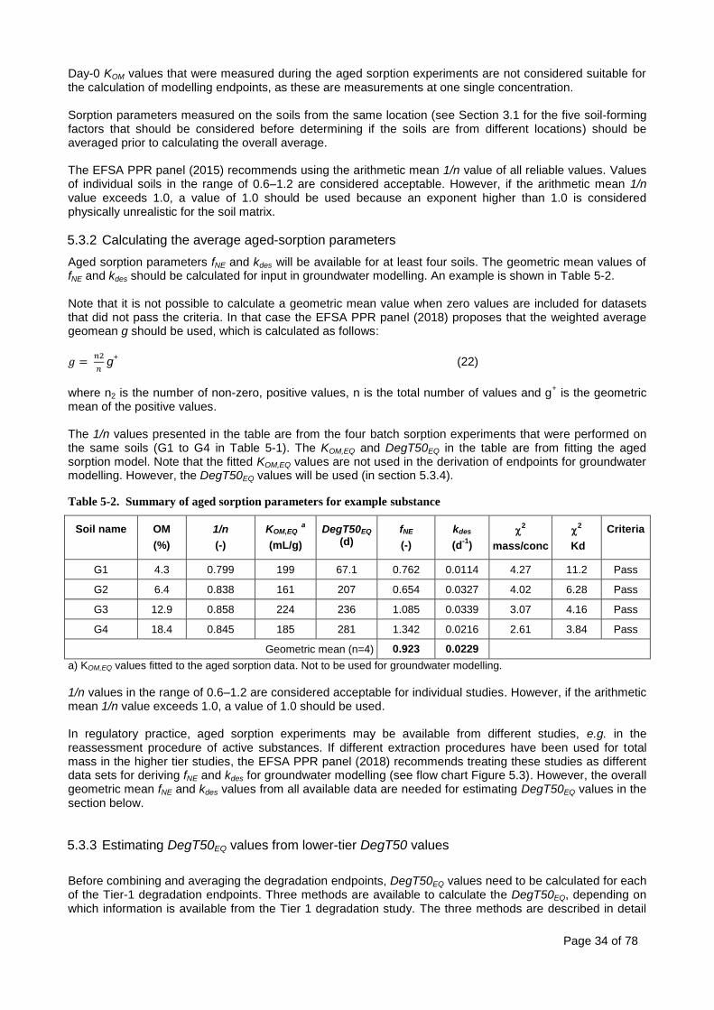
Page 34 of 78

Day-0 KOM values that were measured during the aged sorption experiments are not considered suitable for the calculation of modelling endpoints, as these are measurements at one single concentration. Sorption parameters measured on the soils from the same location (see Section 3.1 for the five soil-forming factors that should be considered before determining if the soils are from different locations) should be averaged prior to calculating the overall average. The EFSA PPR panel (2015) recommends using the arithmetic mean 1/n value of all reliable values. Values of individual soils in the range of 0.6–1.2 are considered acceptable. However, if the arithmetic mean 1/n value exceeds 1.0, a value of 1.0 should be used because an exponent higher than 1.0 is considered physically unrealistic for the soil matrix.

5.3.2 Calculating the average aged-sorption parameters

Aged sorption parameters fNE and kdes will be available for at least four soils. The geometric mean values of fNE and kdes should be calculated for input in groundwater modelling. An example is shown in Table 5-2. Note that it is not possible to calculate a geometric mean value when zero values are included for datasets that did not pass the criteria. In that case the EFSA PPR panel (2018) proposes that the weighted average geomean g should be used, which is calculated as follows:

𝑔 = 𝑛2

𝑛 g

+ (22)

where n2 is the number of non-zero, positive values, n is the total number of values and g+ is the geometric

mean of the positive values. The 1/n values presented in the table are from the four batch sorption experiments that were performed on the same soils (G1 to G4 in Table 5-1). The KOM,EQ and DegT50EQ in the table are from fitting the aged sorption model. Note that the fitted KOM,EQ values are not used in the derivation of endpoints for groundwater modelling. However, the DegT50EQ values will be used (in section 5.3.4).

Table 5-2. Summary of aged sorption parameters for example substance

Soil name OM

(%)

1/n

(-)

KOM,EQ a

(mL/g)

DegT50EQ (d)

fNE

(-)

kdes

(d-1

)

2

mass/conc

2

Kd

Criteria

G1 4.3 0.799 199 67.1 0.762 0.0114 4.27 11.2 Pass

G2 6.4 0.838 161 207 0.654 0.0327 4.02 6.28 Pass

G3 12.9 0.858 224 236 1.085 0.0339 3.07 4.16 Pass

G4 18.4 0.845 185 281 1.342 0.0216 2.61 3.84 Pass

Geometric mean (n=4) 0.923 0.0229

a) KOM,EQ values fitted to the aged sorption data. Not to be used for groundwater modelling.

1/n values in the range of 0.6–1.2 are considered acceptable for individual studies. However, if the arithmetic mean 1/n value exceeds 1.0, a value of 1.0 should be used. In regulatory practice, aged sorption experiments may be available from different studies, e.g. in the reassessment procedure of active substances. If different extraction procedures have been used for total mass in the higher tier studies, the EFSA PPR panel (2018) recommends treating these studies as different data sets for deriving fNE and kdes for groundwater modelling (see flow chart Figure 5.3). However, the overall geometric mean fNE and kdes values from all available data are needed for estimating DegT50EQ values in the section below.

5.3.3 Estimating DegT50EQ values from lower-tier DegT50 values

Before combining and averaging the degradation endpoints, DegT50EQ values need to be calculated for each of the Tier-1 degradation endpoints. Three methods are available to calculate the DegT50EQ, depending on which information is available from the Tier 1 degradation study. The three methods are described in detail

Page 35 of 78

below in order of decreasing ability to describe a soil-specific conversion (and on a decreasing demand for information):

The EFSA PPR panel (2018) recommends that a refit of the aged sorption model to the original data (total mass only) is always the preferred option for the conversion of lower-tier degradation endpoints. If raw data and sufficient information from the Tier 1 study are not available for the performance of an inverse optimisation, scaling factor method 1 is recommended, and finally if not all information for this method is accessible, scaling factor method 2 is to be used. Scaling factors 1 and 2 are based on the equation proposed by Boesten-van der Linden (2001). As pointed out by the EFSA PPR panel (EFSA, 2015), this equation results in an approximate estimation of the DegT50EQ. The equations were tested on a range of existing datasets (Van Beinum et al., 2016), and additional correction factors of 1.1 and 1.2 were added to scaling factors 1 and 2, respectively. These additional correction factors were checked following the revisions to the parameter optimisation recommended by EFSA (2018) and found still to be valid. The scaling factors can be applied before or after normalisation for moisture and temperature. Scaling factor 1 is the full equation and is proposed as the second option. Scaling factor 2 is overall more conservative due to the additional correction factor of 1.2. Scaling factor 2 is a good alternative when there is not sufficient information to calculate scaling factor 1, for example when there is no information on the organic carbon /organic matter content of the soil used in the degradation experiment. For first-tier soils with an additional CaCl2 extraction the EFSA PPR panel (2018) recommends not to use the refit or the scaling factor 1 or 2 approaches, but to directly use the fitted DegT50EQ from the aged sorption fitting procedure, since it is the best estimate for this parameter. However, if the aged sorption model fit did not lead to acceptable parameters, then the DegT50EQ should be estimated from the DegT50 using one of the three methods described below. For first-tier soils without an additional CaCl2 extraction, the geometric mean fNE and kdes parameters should be derived from all available higher-tier studies and used alongside options 1, 2 or 3 in a tiered approach outlined below.

1. Refit of residue data A model, for example PEARLNEQ, can be used to estimate DegT50EQ values for lower-tier degradation study data, in an analogous way to a full aged sorption evaluation but using the geometric mean fNE and kdes parameters derived from the aged sorption studies, according to the following procedures:

Calculate the Total mass degradation data at each timepoint in µg. If not directly available, then the Total mass data can be derived from the %applied radioactivity data and the mass dosed into the test system (µg). The EFSA PPR panel (2018) does not recommend adding the non-extractable residue fraction and possible metabolite to the compound at sampling time t = 0, as is required for kinetic analysis of first-tier degradation studies (FOCUS, 2006).

A PEARLNEQ input file is created using the Total mass data (µg) with inverse optimisation for unweighted data as recommended by the EFSA PPR panel (2018). This is in line with current guidance for first-tier degradation studies (FOCUS, 2006). For the aqueous phase, input ‘dummy values e.g. -99.999’ along with a weighting of zero for all timepoints

Set the volume of liquid added to zero. Set the volume of liquid in soil, mass of soil and organic matter content as usual.

Derive the weighted geometric mean fNE and kdes parameters from the aged sorption studies and fix these in PEARLNEQ

If soil-specific KOC/OM (and 1/n) data are available, then the measured KOM and 1/n are used directly in PEARLNEQ. Otherwise, the overall geometric mean KOM and average 1/n values are used (the average 1/n must not exceed 1). KOM and 1/n are fixed for the evaluation and not optimised

Optimise DegT50EQ and Mini in PEARLNEQ. The optimisation settings in PEARLNEQ should be the same as for standard aged-sorption fitting (see Section 4.4.3).

Calculate the 2-error for unweighted observations using equation 19. Degrees of freedom are

calculated as number of time points minus 2 fitted parameters (Mp ini, DegT50EQ). Calculate RSE of the DegT50EQ using equation 20.

Fits are generally considered acceptable if the 2-error is ≤15% and the RSE value is ≤0.4. The re-

fit essentially draws a line through the total mass data that is based on average kdes and fNE from other soils. This line is not expected to give a perfect fit of the measurements and some deviations are acceptable. The re-fit is an adjustment of the DegT50 that is more accurate than scaling factors, but it is nonetheless an approximation. However, the re-fit should be assessed more critically if SFO

Page 36 of 78

kinetics were rejected at the Tier 1 evaluation of the data and the Tier 1 endpoint is a pseudo-SFO DegT50 derived from the slow phase degradation rate constant or DegT90/3.32. Inclusion of aged sorption during the re-fit may account for the bi-phasic behaviour and yield an acceptable match of the data. But if the visual pattern indicates a strong bi-phasic behaviour and this cannot be

described with the average aged sorption parameters (i.e. if 2-error >15% and/or RSE >0.4), then

the re-fit should be rejected. The pseudo-SFO endpoint should then be adjusted using the scaling

factors described below. Re-fits with large 2-errors or RSE values due to scatter can be accepted.

Normalise DegT50EQ to FOCUS reference conditions (20oC and pF2). PEARLNEQ v5 offers an

option to perform temperature normalisation. However, the EFSA PPR panel (2018) argues that this procedure is prone to error and therefore recommends performing the normalisation of DegT50EQ to the reference temperature outside PEARLNEQ (in the same way a laboratory DegT50 would be normalised). In PEARLNEQ this is achieved by setting the reference temperature to the incubation temperature.

.

2. Scaling factor 1 The lower-tier modelling endpoint DegT50 value is corrected using a scaling factor based on the geometric mean fNE derived from the aged sorption experiment evaluations, w (incubation moisture content, cm

3 / cm

3),

batch KOM and fOM (organic matter fraction) according to the following equation:

𝐷𝑒𝑔𝑇50𝐸𝑄 = 𝐷𝑒𝑔𝑇50 ∗1.1 ∗ (𝑤 + 𝐾𝑂𝑀 ∗ 𝑓𝑂𝑀)

𝑤 + (1 + 𝑓𝑁𝐸) ∗ 𝐾𝑂𝑀 ∗ 𝑓𝑂𝑀 (23)

with the limitation that the calculated DegT50EQ <= DegT50. If the estimated DegT50EQ is greater than the measured DegT50, then set DegT50EQ = DegT50 If a batch OECD106 KOC value is available for the soil, then the soil-specific KOM should be used directly in the estimation (KOM = KOC/1.724). Where no soil-specific KOC data is available, KOM can be calculated from the overall geometric mean KOC. The incubation soil moisture content (w) should be available from the soil degradation study reports and used directly. Where no information is available for w, an alternative is to select the FOCUS default pF2 soil moisture content based on soil texture. If the lower tier endpoint is a pseudo-SFO DegT50 derived from the slow phase degradation rate constant or DegT90/3.32, then this value should be used in equation 23.

3. Scaling factor 2

The lower-tier modelling endpoint DegT50 value is corrected using a simplified scaling factor based on the geometric mean fNE derived from the aged sorption experiment evaluations according to the following equation:

𝐷𝑒𝑔𝑇50𝐸𝑄 = 𝐷𝑒𝑔𝑇50 ∗1.2

(1 + 𝑓𝑁𝐸) (24)

with the limitation that the calculated DegT50EQ <= DegT50. For this conservative approach, fNE values < 0.2 will result in the unrealistic situation that the estimated DegT50EQ is > the measured DegT50. For fNE values < 0.2 the DegT50EQ should therefore be set to the measured DegT50. If the lower tier endpoint is a pseudo-SFO DegT50 derived from the slow phase degradation rate constant or DegT90/3.32, then this value should be used in equation 23.

Page 37 of 78

5.3.4 Calculating average degradation endpoints

After deriving equivalent DegT50EQ values from the lower-tier DegT50 values, all DegT50EQ values are combined for calculation of a geometric mean DegT50EQ. Duplication should be avoided, so only one endpoint should be included per experimental dataset. For example, if a robust DegT50EQ can be directly derived from the aged sorption dataset, then only this value should be used. No additional DegT50EQ should be derived from the lower tier data (DegT50) from this individual experiment using the methods described in Section 5.3.3. Care should be taken when the same incubation study was used to serve as standard degradation study for lower-tier DegT50 values, and as aged sorption study at the higher tier (by performing an additional extraction step with CaCl2-solution). The results are considered the same dataset and should therefore only be included once at each tier when calculating the average degradation endpoints. DegT50EQ values from experiments with the same soil (soils that would be considered the same soil in the regulatory process, e.g. based on source location and/or soil properties, see Section 3.1) should be averaged (using the geometric mean) before calculating the overall geometric mean. 5.3.4.1 Flow charts for combining Tier 1 and aged sorption studies

Aged sorption is a higher-tier approach in the revised FOCUS groundwater guidance (European Commission, 2014). Tier 1 consists of the nine FOCUS standard scenarios. Degradation rates may be from either laboratory or normalised degradation rates from field dissipation studies. Tier 2 consists of more refined modelling approaches. Tier 2a consists of modelling with refined parameters. This includes providing data on specific processes including aged sorption. Tier 2b consists of modelling with refined scenarios. The EFSA PPR panel (2018) recommends combining all available lower-tier degradation and adsorption parameters with the parameters from the aged sorption studies obtained at Tier 2a for use in the groundwater leaching assessment. Furthermore, the EFSA PPR panel (2018) recommends merging aged sorption studies into the same set of soils only if the same extraction procedure was employed. Figure 5-2 illustrates the flow chart that must be applied to combine the parameters of Tier 1 and the aged sorption studies (Tier 2a) in the case that all soils in the higher-tier experiments were extracted with the same procedure for the determination of total mass (one set of parameters). The boxes on the left side represent the first and higher-tier studies, each of them directing to their resulting parameter(s). The first-tier DegT50 values need to be converted to DegT50EQ values in an appropriate way and normalised before averaging. No normalisation is applied to any of the other parameters. The calculated PECgw values can be directly used in groundwater leaching assessments. Figure 5-2. Flow chart for combining Tier 1 and Tier 2a (aged sorption) parameters for groundwater leaching assessment in the case that all soils in the aged sorption study were extracted with the same procedure for the determination of total mass

Page 38 of 78

Figure 5-3 illustrates the flow chart that must be applied to combine the parameters of the first-tier and the aged sorption studies (Tier 2a) in the case that the soils in the higher-tier studies were extracted with two different procedures for the determination of total mass (two sets of parameters). For the aged sorption parameters (fNE and kdes), a check for the extraction procedure assigns the parameters to either set 1 (extraction procedure 1) or to set 2 (extraction procedure 2). These sets are combined with the available DegT50EQ (Tier 1 and aged sorption values), KFOM and 1/n value parameters, which are derived independently of the extraction procedure. PECgw calculations should be performed for each data set and the worst-case value for each scenario is used in groundwater leaching assessment. The flow chart can be easily extended to account for aged sorption studies with three or even more different extraction procedures for the determination of total mass. The conversion of lower tier DegT50 to DegT50EQ by re-fitting or scaling is always based on geomean fNE and kdes values calculated over all studies (i.e. all extraction methods combined). Figure 5-3. Flow chart for combining Tier 1 and Tier 2a (aged sorption) parameters for groundwater leaching assessment in the case that the soils in the aged sorption studies were extracted with two different procedures for the determination of total mass

Page 39 of 78

If agreed soil bulk matrix DegT50 values from field studies have been derived according to EFSA (2014), the EFSA PPR panel (2018) recommends that these values should not be ignored but accounted for in the leaching assessment in line with EFSA (2014). This includes checking whether laboratory and field degradation data are from different populations. To keep consistency with EFSA (2014), this check should be carried out based on soil bulk matrix DegT50 values instead of DegT50EQ values. If lower tier laboratory DegT50 values are not yet available for the aged sorption experiments, then they need to be calculated by fitting degradation kinetics to the total mass data from the aged sorption study using standard FOCUS kinetics procedures. These laboratory DegT50 values are then combined with other lower tier laboratory DegT50 values and compared with matrix DegT50 values from field studies. There are two options (see Figure 5-4):

• If, according to EFSA (2014), the laboratory and field DegT50 are shown to be from the same population, the EFSA PPR panel (2018) recommends that field DegT50 values be converted into appropriate DegT50EQ values using the second scaling factor unless a soil-specific water holding capacity (measured at pF 2) is available, in which case scaling factor 1 should be used. Note that deriving field DegT50EQ by kinetic analysis of the field data using aged sorption parameters from the laboratory is currently not recommended by EFSA (EFSA, 2018).

• If field DegT50 values represent a different population, and the field DegT50 values are statistically shorter than the laboratory DegT50 values, the EFSA PPR panel (2018) considers that rescaling the field DegT50 data on the basis of laboratory aged sorption data is not justifiable because there is no experimental evidence that the extent of aged sorption in the laboratory and in the field is the same. So, in this particular case, the EFSA PPR panel (2018) recommends using the field DegT50 values together with the laboratory aged sorption data in the leaching assessment without scaling the field DegT50 values as a conservative approach. In the unlikely event that the field DegT50 values are statistically longer than the laboratory DegT50 values, the reasons should be investigated, and action taken as described in the EFSA DegT50 guidance (2014). If the DegT50 from the lab aged sorption is greater than 240 days, then no comparison is made between the lab DegT50 and field DegT50 (as per EFSA (2014) guidance). In this situation,

Page 40 of 78

only the field DegT50, with no correction factor, should be taken forward for use in the aged sorption model.

These recommendations from the EFSA PPR Panel (2018) are intended to add some additional conservatism because currently there is no experimental evidence that the extent of aged sorption in the laboratory and field are the same. However, these recommendations were untested. Preliminary tests by the authors suggest that following these recommendations can, in some circumstances, result in higher PECGW values than first-tier groundwater modelling and therefore the definition of a tiered approach is not met. This is because PEC modelling with aged sorption assumes that degradation only occurs in the equilibrium domain. Using the uncorrected field DegT50 value for the equilibrium domain and zero degradation for the non-equilibrium domain leads to greater persistence than a tier 1 simulation where degradation is described by the field DegT50. The increase in sorption over time does not always compensate for the increase in persistence. The following recommendation is therefore made:

• In circumstances where the implementation of these two EFSA PPR Panel (2018) recommendations results in higher PECGW values than using the first-tier (non-aged sorption) approach, the PECGW results from the aged sorption assessment should still be provided but may be omitted by Regulators from use in the risk assessment. However, in this situation, where studies have been submitted to derive aged sorption parameters, the DegT50 values derived from the total mass data in the specific aged sorption experiment should be incorporated into the overall DegT50 dataset to determine whether the laboratory and field DegT50 values are from the same population (following the EFSA DegT50 guidance, 2014).

Figure 5-4. Flow chart for combining field degradation and laboratory degradation data

The PPR Panel (2018) considers that ideally the aged sorption parameters and the field degradation half-lives would be obtained simultaneously using inverse modelling. Industry are preparing evidence for aged sorption in field studies and this option should replace the current recommendations as soon as appropriate guidance has been developed and tested.

5.4 Groundwater modelling

Page 41 of 78

Groundwater PEC calculations can be performed in any of the FOCUS groundwater models: FOCUS PEARL (all versions), FOCUS_PELMO (version 4.4.3 and up) and FOCUS_PRZM (version 3.5.2 and up) and FOCUS_MACRO (version 5.5.3 and up). For use in FOCUS_MACRO, the parameters fNE and kdes must be converted into MACRO parameters using Equations 9 and 11 (see Section 4.2).

6 Special considerations for metabolites

In the context of typical regulatory submissions, the fate of metabolites can be investigated in soils treated with the parent compound. Alternatively, they can be added directly to the soil. In the case of determining aged sorption parameters for metabolites, the EFSA PPR panel (2018) recommends aged sorption parameters are only obtained from metabolite dosed studies. Recent research (Defra, 2015) showed that it is difficult to derive reliable parameters for metabolites that are formed during the experiment, unless the parent compound degraded quickly. The recommendations from this research project are summarised in Appendix 7. It is recommended therefore that aged sorption parameters for metabolites should only be derived from experiments in which metabolite is applied to the soil. Then the same requirements and criteria apply for aged sorption of metabolites as described in the guidance for parent compounds. There is an additional issue that needs to be considered when aged sorption parameters for metabolites are used in regulatory leaching assessments:

• If leaching of the parent and metabolite is calculated simultaneously in a leaching model, a formation fraction for the metabolite must be entered into the model. This cannot be derived from the aged sorption study and must be obtained from a degradation study with the parent compound as the added substance. EFSA (2018) implied that metabolite formation fractions must be derived by fitting the total mass of the substances which exhibit aged sorption with the DFOP model. This is because pronounced aged sorption can result in a bi-phasic decline of the total mass.

Clarification from the authors of the EFSA PPR Opinion (2018) in a personal capacity made clear that it is not foreseen to re-fit metabolite data from lower tier studies with the DFOP model because this will rarely give a reliable fit for the metabolite and the impact on the formation fraction is likely to be minor. Therefore, the formation fraction from the metabolite should be taken from the parent-metabolite kinetic assessment according to FOCU (2006; 2014).

If the parent shows signs of aged sorption and single-first order (SFO) kinetics for the parent are deemed adequate to derive lower tier modelling endpoints, then refitting of the dataset with the DFOP model for the parent may be considered in order to derive a robust formation fraction for the metabolite. If the DFOP re-fit for the parent does not give robust parameters, then the endpoints from an SFO model can be used.

Page 42 of 78

7 References

Altfelder, S., Streck, T., and Richter, J. (1999). Effect of air-drying on sorption kinetics of the herbicide chlortoluron in soil. Journal of Environmental Quality, 28, 1154–1161.

Boesten, J.J.T.I., and van der Linden, A.M.A. (2001). Effect of long-term sorption kinetics on leaching as calculated with the PEARL model for FOCUS scenarios. BCPC Symposium Proceedings No.78: Pesticide Behaviour in Soils and Water.

Boesten, J.J.T.I., Tiktak, A., and van Leerdam R.C. (2007). Manual of PEARLNEQ v4. ALTERRA, Wageningen: WOT Natuur & Milieu (Workdocuments 71) 34 pp.

Boesten, J.J.T.I., van der Linden, A.M.A., Beltman W.H.J., and Pol, J.W. (2011). Leaching of plant protection products and transformation products; Proposals for improving the assessment of leaching to groundwater in the Netherlands – Version 2 (Alterra report 2630).

Cox, L. and Walker, A. (1999). Studies of time-dependent sorption of linuron and isoproturon in soils. Chemosphere 38:2707-2718.

Defra (2004). Time-dependent sorption processes in soil. Report for Defra project PS2206. Warwick HRI. http://randd.defra.gov.uk/Document.aspx?Document=PS2206_3831_FRP.doc

Defra (2009). Characterisation and modelling of time-dependent sorption of pesticides. Report for Defra project PS2228. The Food and Environment Research Agency.

http://randd.defra.gov.uk/Document.aspx?Document=PS2228_7878_FRP.doc

Defra (2010). Development of guidance on the implementation of aged soil sorption studies into regulatory exposure assessments. Report for Defra project PS2235. The Food and Environment Research Agency.

Defra (2012). Consideration of additional experimental datasets to support the development of the revised guidance on aged sorption studies. Report for Defra project PS2244. The Food and Environment Research Agency.

Defra (2015). Use of field data to generate aged sorption parameters for regulatory leaching assessments. Report for Defra project PS2254. The Food and Environment Research Agency.

Defra (2016). Additional testing and revision of the draft guidance on aged sorption. Enviresearch Report E2016-30. 45pp.

Doherty (2005). PEST. Model-independent parameter estimation. 5th edition. Watermark Numerical

Computing. www.sspa.com/pest, version 9.01. http://www.pesthomepage.org/files/pestman.pdf

EC (2014a). Assessing potential for movement of active substances and their metabolites to ground water in the EU. Report of the FOCUS ground water work group, EC Document Reference SANCO/13144/2010 version 3, 613 pp.

EC (2014b). Generic guidance for Tier 1 FOCUS ground water assessments. Version 2.2. EC Document Reference SANCO/321/2000 rev.2 version 2.2, 66p.

EFSA (2014). EFSA Guidance document for evaluating laboratory and field dissipation studies to obtain DegT50 values of active substances of plant protection products and transformation products of these active substances in soil. EFSA Journal 12(5): 3662, 37 pp.

EFSA (2015). Statement on the FERA guidance proposal: ‘Guidance on how aged sorption studies for pesticides should be conducted, analysed and used in regulatory assessments’ (FERA, 2012). EFSA Journal 2015: 13(7):4175, 54 pp.

EFSA (2017). Technical report on the outcome of the pesticides peer review meeting on the OECD 106 evaluators checklist. EFSA supporting publication 2017:EN-1326, 17 pp.

EFSA (2018). Scientific Opinion about the Guidance of the Chemical Regulation Directorate (UK) on how aged sorption studies for pesticides should be conducted, analysed and used in regulatory assessments. EFSA Journal 2018; 16(8);5382, 86 pp.

FOCUS (2006). Guidance document on estimating persistence and degradation kinetics from environmental fate studies on pesticides in EU registration, report of the FOCUS work group on degradation kinetics, EC document reference Sanco/10058/2005 Version 2.0, 434 pp.

FOCUS (2014). Generic Guidance for Estimating Persistence and Degradation Kinetics from Environmental Fate Studies in Pesticides in EU Registration (version 1.1) EC Document Reference Sanco/10058/2005 version 2.0, 434 pp.

Hardy, I. A. J. (2011). Evaluation of aged-sorption studies: testing of the draft guidance. Battelle report number PS/10/001A. 94p.

Page 43 of 78

Gao, Z., Green J.W., Vanderborght, J. and Schmitt W. (2011). Improving Uncertainty Analysis in Kinetic Evaluations Using Iteratively Reweighted Least Squares. Environmental Toxicology and Chemistry 30:2263-2271.

Görlitz, L., Gao, Z, Schmitt, W. (2011), Statistical Analysis of Chemical Transformation Kinetics using Markov-Chain Monte-Carlo Methods. Environmental Science and Technology 45:4429–4437

Gurney, A.J.R. and Hayes, S.E. (2007). Non-equilibrium sorption and degradation of pesticides in soil: analysis of laboratory aged sorption data using ModelMaker. In: A.A.M. Del Re, E. Capri, G. Gragoulis, and M. Trevisan, eds. Environmental Fate and Ecological Effects of Pesticides (Proceedings of the XIII Symposium Pesticide Chemistry). La Goliardica Pavese, Pavia Italy, ISBN 978-88-7830-473-4, pp. 245-253.

Leistra, M., Van der Linden, A.M.A., Boesten, J.J.T.I., Tiktak, A. and Van den Berg, F. (2001). PEARL model for pesticide behaviour and emissions in soil-plant systems. Description of processes. Alterra report 013, Alterra, Wageningen, RIVM report 711401009, Bilthoven, The Netherlands. Available at http://www.pearl.pesticidemodels.eu.

Larsbo, M. and Jarvis, N. (2003). MACRO 5.0. A model of water flow and solute transport in macroporous soil. Technical description. Report. Department of Soil Science. Swedish University of Agricultural Sciences. 49 pp.

MatLab (2007). MatLab Version 7.4.0.287 (R2007a), Optimisation Toolbox, Statistics Toolbox, MatLab Compiler. The MathWorks Inc., USA. www.mathworks.com

OECD (2000). OECD Guidelines for the Testing of Chemicals. Test No 106: “Adsorption-Desorption using a Batch Equilibrium Method” - Organization for Economic Cooperation and Development.

OECD (2002). OECD Guidelines for the Testing of Chemicals. Test No 307: Aerobic and anaerobic transformation in soil. Organization for Economic Cooperation and Development.

Streck, T., Poletika N.N., Jury, W.A. and Farmer,W.J. (1995). Description of simazine transport with rate-limited,two-stage, linear and nonlinear sorption. Water Resources Research 31:811-822.

Sur, R., Menke, U., Dalkmann, P., Paetzold, S., Keppler, J. and Goerlitz, G. (2009). Comparative evaluation of time-dependent sorption data of pesticides. Proceedings of the Conference on Pesticides in Soil, Water and Air, 12-14 September 2009, York, UK.

Van Beinum, W., Beulke, S. and Hardy I. A. J. (2016). Further testing in support of the guidance on aged sorption. Enviresearch Report Number: E2016-35. Battelle Report Number: PS/16/001A.

Walker, A. and Jurado-Exposito, M. (1998). Adsorption of isoproturon, diuron and metsulfuron-methyl in two soils at high soil:solution ratios. Weed Research 38:229-238.

Wauchope, R.D., Yeh, S., Linders, J.B.H.J., Kloskowski, R., Tanaka, K., Rubin, B., Katayama, A, Kordel, W., Gerstl, Z., Lane, M. and Unsworth J.B. (2002). Pesticide soil sorption parameters: theory, measurement, uses, limitations and reliability. Pest Management Science 58:419-445.

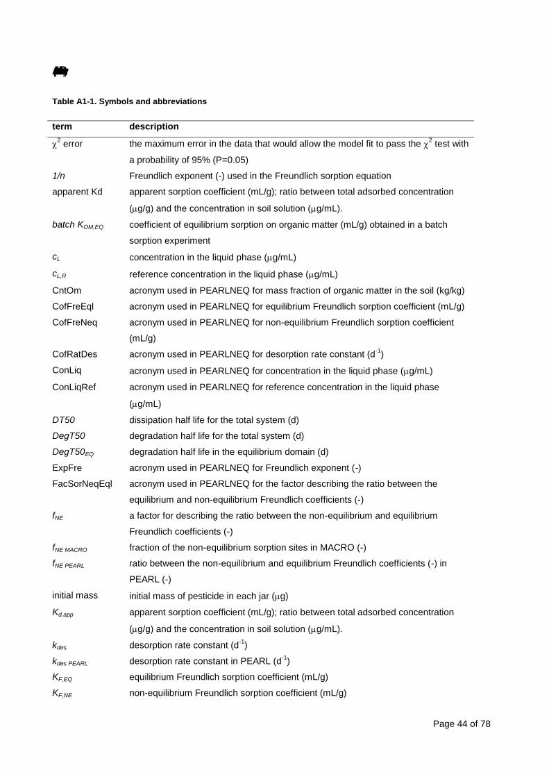
Page 44 of 78

Appendix 1. Glossary

Table A1-1. Symbols and abbreviations

term description

2 error the maximum error in the data that would allow the model fit to pass the

2 test with

a probability of 95% (P=0.05)

1/n Freundlich exponent (-) used in the Freundlich sorption equation

apparent Kd apparent sorption coefficient (mL/g); ratio between total adsorbed concentration

(g/g) and the concentration in soil solution (g/mL).

batch KOM,EQ coefficient of equilibrium sorption on organic matter (mL/g) obtained in a batch

sorption experiment

cL concentration in the liquid phase (g/mL)

cL,R reference concentration in the liquid phase (g/mL)

CntOm acronym used in PEARLNEQ for mass fraction of organic matter in the soil (kg/kg)

CofFreEql acronym used in PEARLNEQ for equilibrium Freundlich sorption coefficient (mL/g)

CofFreNeq acronym used in PEARLNEQ for non-equilibrium Freundlich sorption coefficient

(mL/g)

CofRatDes acronym used in PEARLNEQ for desorption rate constant (d-1

)

ConLiq acronym used in PEARLNEQ for concentration in the liquid phase (g/mL)

ConLiqRef acronym used in PEARLNEQ for reference concentration in the liquid phase

(g/mL)

DT50 dissipation half life for the total system (d)

DegT50 degradation half life for the total system (d)

DegT50EQ degradation half life in the equilibrium domain (d)

ExpFre acronym used in PEARLNEQ for Freundlich exponent (-)

FacSorNeqEql acronym used in PEARLNEQ for the factor describing the ratio between the

equilibrium and non-equilibrium Freundlich coefficients (-)

fNE a factor for describing the ratio between the non-equilibrium and equilibrium

Freundlich coefficients (-)

fNE MACRO fraction of the non-equilibrium sorption sites in MACRO (-)

fNE PEARL ratio between the non-equilibrium and equilibrium Freundlich coefficients (-) in

PEARL (-)

initial mass initial mass of pesticide in each jar (g)

Kd,app apparent sorption coefficient (mL/g); ratio between total adsorbed concentration

(g/g) and the concentration in soil solution (g/mL).

kdes desorption rate constant (d-1

)

kdes PEARL desorption rate constant in PEARL (d-1

)

KF,EQ equilibrium Freundlich sorption coefficient (mL/g)

KF,NE non-equilibrium Freundlich sorption coefficient (mL/g)

Page 45 of 78

KF,Total sum of equilibrium plus non-equilibrium Freundlich sorption coefficient (mL/g)

KOC sorption coefficient for sorption on soil organic carbon (mL/g org. carbon)

KOM sorption coefficient for sorption on soil organic matter (mL/g org. matter)

KOM,EQ coefficient of equilibrium sorption on organic matter (mL/g)

KomEql acronym used in PEARLNEQ for coefficient of equilibrium sorption on organic

matter (mL/g)

kt degradation rate constant (d-1

) in the equilibrium domain

LOQ limit of quantification; smallest concentration at which the substance concentration

can be quantified in a certain medium

Mas acronym used in PEARLNEQ for total mass of pesticide in each jar (g)

MasSol acronym used in PEARLNEQ for the mass of soil (dry weight) incubated in each jar

(g)

mOM mass fraction of organic matter in the soil (g/g)

Mp total mass of pesticide in each jar (g)

Mp ini initial mass of pesticide in each jar (g)

Ms the mass of soil (dry weight) incubated in each jar (g)

mwhc maximum water holding capacity of the soil

PECGW

phi

Predicted Environmental Concentration in groundwater

sum of squared residuals between the measured data and the simulated values in

PEARLNEQ

RSE relative standard error for the estimated parameter value

SSQ sum of squared residuals between the measured data and the simulated values

V the volume of water in the soil incubated in each jar (mL)

VolLiq acronym used in PEARLNEQ for the volume of water in the soil incubated in each

jar (mL)

w incubation moisture content (mL/g)

XEQ pesticide mass sorbed at equilibrium sites (g/g)

XNE pesticide mass sorbed at non-equilibrium sites (g/g)

XNeq acronym used in PEARLNEQ output file for pesticide mass sorbed at non-

equilibrium sites (g/g)

αMACRO desorption rate constant (d-1

) used in MACRO.

Page 46 of 78

Table A1-2. Terms and definitions

term description

aged sorption increased sorption after extended contact between pesticide and soil

aged sorption study incubation study whereby sorption is measured at different time

intervals after application of the test substance

batch sorption study sorption study in which soils are shaken with pesticide solution for a

certain period of time

equilibrium domain the liquid phase and the equilibrium sorption sites together

equilibrium sorption sites locations in the soil where sorption occurs rapidly. In the two-site

model this part of sorption is assumed to reach equilibrium

instantaneously, while non-equilibrium sorption is the additional

sorption that takes place with prolonged contact time. The cut-off

between equilibrium and non-equilibrium sorption is arbitrary. Here

equilibrium sorption is defined as the sorption that would occur after

24 hours shaking of the soil with pesticide solution.

legacy study Experiment that was performed before this guidance came into use,

or during the agreed implementation period

non-equilibrium sorption sites locations in the soil where sorption occurs with time, when the

pesticide is exposed to the soil for a longer period. See also the

description of ‘equilibrium sorption sites’. In this guidance non-

equilibrium sorption is defined as the sorption that occurs beyond

equilibrium sorption.

recovery percentage of test compound that can be recovered from the soil by

extraction

two-site model a model that describes sorption on two types of sorption sites:

equilibrium sites and non-equilibrium sites. Sorption on the

equilibrium sites is assumed to reach equilibrium instantaneously,

while adsorption and desorption on the non-equilibrium sites take

time to reach equilibrium.

Page 47 of 78

Appendix 2: Fitting of a two-site model with PEARLNEQ to two example datasets

Example 1

An aged sorption laboratory incubation study was carried out using the experimental design described in Chapter 3 of this guidance. The experimental conditions are shown in Table A2-1 and the measurements are given in Table A2-2. Table A2-1. Experimental conditions of the laboratory aged sorption study (example 1)

Parameter Unit Value

Applied mass of pesticide µg 20 Mass of dry soil g 8.52 Moisture mL 1.48 Volume of added CaCl2 solution mL 20 Organic carbon (OC) % 1.47 Organic matter (OM) % 2.53 Temperature

oC

20

Limit of quantification in soil µg g-1

0.45 Limit of quantification in CaCl2 µg mL

-1 0.026

KF,OM, (batch equilibrium sorption study) mL g-1

246 Freundlich exponent 1/n (batch equilibrium sorption study) - 0.830

Table A2-2. Measured data and calculated sorption and apparent Kd values (example 1)

time Total extracted residue

Concentration in CaCl2 solution

Adsorbed Apparent Kd

(days) (µg) (µg mL-1

) (µg g-1

) (mL g-1

)

0.1 20.18 0.2346 1.78 7.57

0.1 20.40 0.2304 1.81 7.87

0.1 20.09 0.2321 1.77 7.64

1.0 20.29 0.2243 1.82 8.10

1.0 20.31 0.2231 1.82 8.16

1.0 20.38 0.2212 1.83 8.29

3.1 19.19 0.1830 1.79 9.79

3.1 19.12 0.1871 1.77 9.48

3.1 18.93 0.2009 1.72 8.54

7.1 18.74 0.1843 1.73 9.41

7.1 18.58 0.1831 1.72 9.38

7.1 18.23 0.1780 1.69 9.50

14.1 17.49 0.1678 1.63 9.71

14.1 17.60 0.1647 1.65 10.02

14.1 17.85 0.1632 1.68 10.32

28.0 16.23 0.1295 1.58 12.19

28.0 16.20 0.1287 1.58 12.25

28.0 16.26 0.1271 1.59 12.50

43.1 14.93 0.1128 1.47 13.01

43.1 14.99 0.1083 1.49 13.73

43.1 15.23 0.1089 1.51 13.90

57.1 13.85 0.0947 1.39 14.64

57.1 13.78 0.0911 1.39 15.24

57.1 13.71 0.0966 1.37 14.14

71.1 13.61 0.0850 1.38 16.28

71.1 13.17 0.0821 1.34 16.30

71.1 12.80 0.0896 1.28 14.24

82.0 12.49 0.0799 1.26 15.81

82.0 12.42 0.0792 1.26 15.88

82.0 11.93 0.0793 1.20 15.14

Page 48 of 78

All measured values are above the LOQ, so all are included in the modelling. Sorption at each time point was calculated from the measurements as:

𝐴𝑑𝑠𝑜𝑟𝑏𝑒𝑑 𝑎𝑚𝑜𝑢𝑛𝑡 [𝜇𝑔 𝑔−1]

=𝑇𝑜𝑡𝑎𝑙 𝑟𝑒𝑠𝑖𝑑𝑢𝑒 [𝜇𝑔] − (𝐶𝑜𝑛𝑐𝑒𝑛𝑡𝑟𝑎𝑡𝑖𝑜𝑛 𝑖𝑛 𝐶𝑎𝐶𝑙2 𝑠𝑜𝑙𝑢𝑡𝑖𝑜𝑛 [𝜇𝑔 𝑚𝐿−1] × 𝑉𝑜𝑙𝑢𝑚𝑒 𝑜𝑓 𝑙𝑖𝑞𝑢𝑖𝑑[𝑚𝐿])

𝑀𝑎𝑠𝑠 𝑜𝑓 𝑠𝑜𝑖𝑙 [𝑔]

Note that ‘volume of liquid’ refers to the total volume of liquid during the extraction with CaCl2 solution (soil solution plus added CaCl2-solution). In this example the total volume of liquid was 1.48 + 20 mL =21.48 mL and the dry mass of soil was 8.52 g. The first line of the table shows a concentration in CaCl2 solution of 0.2346 µg/ml and the total extracted pesticide residue in the same soil sample was 20.18 µg. This gives an adsorbed amount of 1.78 µg/g. The apparent Kd in Table A2-2 was calculated for each measurement as:

𝐾𝑑,𝑎𝑝𝑝[𝑚𝐿 𝑔−1] =𝐴𝑑𝑠𝑜𝑟𝑏𝑒𝑑 𝑎𝑚𝑜𝑢𝑛𝑡 [𝜇𝑔 𝑔−1]

𝐶𝑜𝑛𝑐𝑒𝑛𝑡𝑟𝑎𝑡𝑖𝑜𝑛 𝑖𝑛 𝐶𝑎𝐶𝑙2 𝑠𝑜𝑙𝑢𝑡𝑖𝑜𝑛 [𝜇𝑔 𝑚𝐿−1]

In order to carry out the non-equilibrium parameter estimation procedure in PEARLNEQ, the .mkn file of the PEARLNEQ package has to be compiled following the instructions in the PEARLNEQ manual. The .mkn file of PEARLNEQ for the example case is shown below. The starting value for the initial mass (‘MasIni’ = 19.55 µg) and DegT50 (‘DT50Ref’ = 117.61 days) were derived by fitting a first-order kinetic model to the mass data. The Freundlich exponent 1/n (‘ExpFre’) and the starting value for KOM,EQ were set to the values measured on the same soil during the batch equilibrium sorption experiments according to OECD Guideline 106. Four starting value combinations were tested for fNE (‘FacSorNeqEql’) and kdes (‘CofRatDes’). In this example, the starting values for fNE were 0.2 and 1.5 and those for kdes were 0.004 d

-1 and 0.05 d

-1. To avoid temperature corrections within PEARLNEQ, ensure that

reference temperature in the .mkn file is set equal to the incubation temperatures. Correction of the degradation half-life to 20

oC must be done outside PEARLNEQ (EFSA, 2018).

PEARLNEQ .mkn file for example case 1

*-----------------------------------------------------------------------------------------

* STANDARD FILE for pearlmk version 5

* Program to fit the half-life, activation energy and parameters for long-term sorption

* kinetics of pesticides in soil

*

* This file is intented for use with the PEST program (Doherty et al., 1991).

* Please refer to the manual of PEARLNEQ

*

* (c) Alterra 2012

*-----------------------------------------------------------------------------------------

* Model control

Yes ScreenOutput

0.0 TimStart (d) Start time of experiment

120.0 TimEnd (d) End time of experiment

0.01 DelTim (d) Time step of Euler's integration procedure

* System characterization

19.55 MasIni (ug) Initial guess of initial mass

8.52 MasSol (g) Mass of soil in incubation jar

1.48 VolLiqSol (mL) Volume of liquid in the moist soil

20.0 VolLiqAdd (mL) Volume of liquid ADDED

0.0253 CntOm (kg.kg-1) Organic matter content

* Sorption parameter

1.0 ConLiqRef (mg.L-1) Reference liquid concentration

0.830 ExpFre (-) Freundlich exponent

246 KomEql (L.kg-1) Freundlich coefficient for equilibrium sorption

0.2 FacSorNeqEql (-) Initial guess of ratio KfNeq/KfEql

0.004 CofRatDes (d-1) Initial guess of desorption rate constant

Neql OptSor (-) Option for type of sorption process to be

simulated: 'Neql' or 'Eql'

* Transformation parameters

117.61 DT50Ref (d) Initial guess of half-life at ref. temperature

Page 49 of 78

20.0 TemRefTra (C) Reference temperature

65.4 MolEntTra (kJ.mol-1) Initial guess of molar activation energy

* Temperature at which the incubation experiments have been carried out

table Tem (C)

1 20.0

end_table

* Number of replicate sets (range 1 - 9)

* A set of replicates can contain observation at different time points and temperatures

* Each replicate set should contain at least one measurement performed at each of the temperatures

specified in table Tem

* 1st sort by Rep. (column 5), 2nd sort by Tem (column 2), 3rd sort by Tim (column 1)

* specify missing values or values you do not want to include in the optimisation procedure (e.g.

outliers) as -99.999

* PEARLMK will give these observations a weight of zero, meaning that the observation takes to part

in the optimisation

3 NumRepSet (-)

* Provide the results of the measurements

* Tim Tem Mas ConLiq Rep. observation ID

* (d) (C) (ug) (ug/mL)

table Observations

0.1 20 20.180 0.23460 1 OBS

1.0 20 20.290 0.22430 1 OBS

3.1 20 19.190 0.18300 1 OBS

7.1 20 18.740 0.18430 1 OBS

14.1 20 17.490 0.16780 1 OBS

28.0 20 16.230 0.12950 1 OBS

43.1 20 14.930 0.11280 1 OBS

57.1 20 13.850 0.09470 1 OBS

71.1 20 13.610 0.08500 1 OBS

82.0 20 12.490 0.07990 1 OBS

0.1 20 20.400 0.23040 2 OBS

1.0 20 20.310 0.22310 2 OBS

3.1 20 19.120 0.18710 2 OBS

7.1 20 18.580 0.18310 2 OBS

14.1 20 17.600 0.16470 2 OBS

28.0 20 16.200 0.12870 2 OBS

43.1 20 14.990 0.10830 2 OBS

57.1 20 13.780 0.09110 2 OBS

71.1 20 13.170 0.08210 2 OBS

82.0 20 12.420 0.07920 2 OBS

0.1 20 20.090 0.23210 3 OBS

1.0 20 20.380 0.22120 3 OBS

3.1 20 18.930 0.20090 3 OBS

7.1 20 18.230 0.17800 3 OBS

14.1 20 17.850 0.16320 3 OBS

28.0 20 16.260 0.12710 3 OBS

43.1 20 15.230 0.10890 3 OBS

57.1 20 13.710 0.09660 3 OBS

71.1 20 12.800 0.08960 3 OBS

82.0 20 11.930 0.07930 3 OBS

end_table

* Option for weights of Observations:

*'equal' gives equal weights to all measurements

*'inverse' gives weigth equal to inverse value of each measurement (if measurement is zero then

weight is 1.0)

inverse Opt_weights

* Option for description of transformation rate

* 'EqlDom' uses rate based on amount of substance in equilibrium domain

* 'LiqPhs' uses rate based on amount of substance in liquid phase

EqlDom Opt_transformation

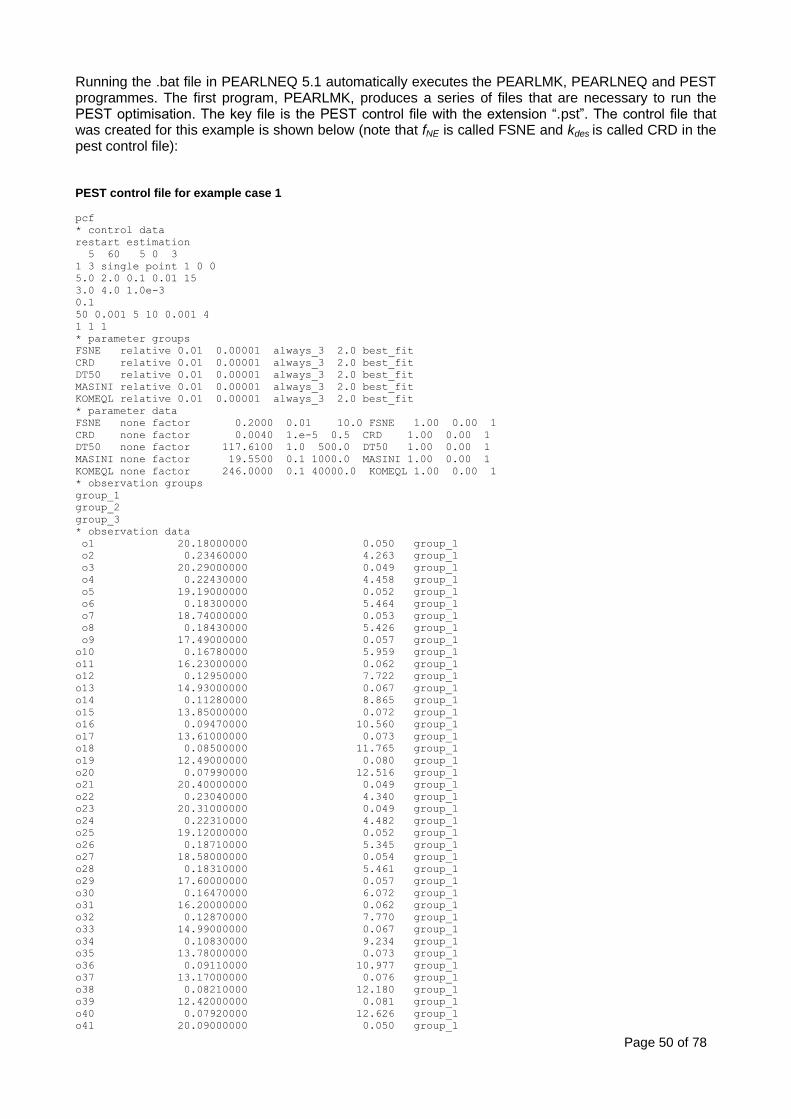
Page 50 of 78

Running the .bat file in PEARLNEQ 5.1 automatically executes the PEARLMK, PEARLNEQ and PEST programmes. The first program, PEARLMK, produces a series of files that are necessary to run the PEST optimisation. The key file is the PEST control file with the extension “.pst”. The control file that was created for this example is shown below (note that fNE is called FSNE and kdes is called CRD in the pest control file): PEST control file for example case 1

pcf

* control data

restart estimation

5 60 5 0 3

1 3 single point 1 0 0

5.0 2.0 0.1 0.01 15

3.0 4.0 1.0e-3

0.1

50 0.001 5 10 0.001 4

1 1 1

* parameter groups

FSNE relative 0.01 0.00001 always_3 2.0 best_fit

CRD relative 0.01 0.00001 always_3 2.0 best_fit

DT50 relative 0.01 0.00001 always_3 2.0 best_fit

MASINI relative 0.01 0.00001 always_3 2.0 best_fit

KOMEQL relative 0.01 0.00001 always_3 2.0 best_fit

* parameter data

FSNE none factor 0.2000 0.01 10.0 FSNE 1.00 0.00 1

CRD none factor 0.0040 1.e-5 0.5 CRD 1.00 0.00 1

DT50 none factor 117.6100 1.0 500.0 DT50 1.00 0.00 1

MASINI none factor 19.5500 0.1 1000.0 MASINI 1.00 0.00 1

KOMEQL none factor 246.0000 0.1 40000.0 KOMEQL 1.00 0.00 1

* observation groups

group_1

group_2

group_3

* observation data

o1 20.18000000 0.050 group_1

o2 0.23460000 4.263 group_1

o3 20.29000000 0.049 group_1

o4 0.22430000 4.458 group_1

o5 19.19000000 0.052 group_1

o6 0.18300000 5.464 group_1

o7 18.74000000 0.053 group_1

o8 0.18430000 5.426 group_1

o9 17.49000000 0.057 group_1

o10 0.16780000 5.959 group_1

o11 16.23000000 0.062 group_1

o12 0.12950000 7.722 group_1

o13 14.93000000 0.067 group_1

o14 0.11280000 8.865 group_1

o15 13.85000000 0.072 group_1

o16 0.09470000 10.560 group_1

o17 13.61000000 0.073 group_1

o18 0.08500000 11.765 group_1

o19 12.49000000 0.080 group_1

o20 0.07990000 12.516 group_1

o21 20.40000000 0.049 group_1

o22 0.23040000 4.340 group_1

o23 20.31000000 0.049 group_1

o24 0.22310000 4.482 group_1

o25 19.12000000 0.052 group_1

o26 0.18710000 5.345 group_1

o27 18.58000000 0.054 group_1

o28 0.18310000 5.461 group_1

o29 17.60000000 0.057 group_1

o30 0.16470000 6.072 group_1

o31 16.20000000 0.062 group_1

o32 0.12870000 7.770 group_1

o33 14.99000000 0.067 group_1

o34 0.10830000 9.234 group_1

o35 13.78000000 0.073 group_1

o36 0.09110000 10.977 group_1

o37 13.17000000 0.076 group_1

o38 0.08210000 12.180 group_1

o39 12.42000000 0.081 group_1

o40 0.07920000 12.626 group_1

o41 20.09000000 0.050 group_1

Page 51 of 78

o42 0.23210000 4.308 group_1

o43 20.38000000 0.049 group_1

o44 0.22120000 4.521 group_1

o45 18.93000000 0.053 group_1

o46 0.20090000 4.978 group_1

o47 18.23000000 0.055 group_1

o48 0.17800000 5.618 group_1

o49 17.85000000 0.056 group_1

o50 0.16320000 6.127 group_1

o51 16.26000000 0.062 group_1

o52 0.12710000 7.868 group_1

o53 15.23000000 0.066 group_1

o54 0.10890000 9.183 group_1

o55 13.71000000 0.073 group_1

o56 0.09660000 10.352 group_1

o57 12.80000000 0.078 group_1

o58 0.08960000 11.161 group_1

o59 11.93000000 0.084 group_1

o60 0.07930000 12.610 group_1

* model command line

..\neq_bin\PearlNeq example

* model input/output

example.tpl example.neq

example1.ins example.out

example2.ins example.out

example3.ins example.out

Next the .bat file starts the execution of the PEST program. PEST performs the optimisation by repeatedly running the PEARLNEQ model. PEARLNEQ produces an output file as shown below. PEST compares the results of the output file against the measured data and changes the parameters. PEST continues running PEARLNEQ until the sum of squared residuals is minimised or the termination criteria specified in the pest control file are met.

Final output file for example case 1, starting value combination 1 (only first page of the output file is shown)

* ------------------------------------------------------------------------------

* Results from PEARLNEQ (c) Alterra

* PEARLNEQ version 5.1

* PEARLNEQ created on 14-August-2012

*

* Run ID : example

* Input file generated on : 19-06-2019

* ------------------------------------------------------------------------------

*

--------------------------------------------------------------

* System properties

* Mass of dry soil (g) : 8.5200

* Volume of water in moist soil (mL) : 1.4800

* Volume of water added (mL) : 20.0000

* Initial mass of pesticide (ug) : 19.8376

* Reference concentration (ug.mL-1) : 1.0000

* Equilibrium sorption coeff (mL.g-1) : 6.1678

* Non-equili. sorption coeff (mL.g-1) : 2.7669

* Freundlich exponent (-) : 0.8300

* Desorption rate coefficient (d-1) : 0.0363

* Half-life transformation (d) : 87.1673

* Half-life based on substance in equilibrium domain

* Arrhenius activation energy (kJ mol-1): 65.4000

* Reference temperature (K) : 293.1500

--------------------------------------------------------------

* Temp Time Mas ConLiq XNeq XEq Kd_app

* (C) (d) (ug) (ug.mL-1) (ug.g-1) (ug.g-1) (mL.g-1)

20.0 0.000 19.83762400 0.22202195 0.00000000 1.76862779 7.96600428

20.0 0.042 19.83105392 0.22176859 0.00154291 1.76695248 7.97450797

20.0 0.083 19.82449037 0.22151578 0.00308197 1.76528044 7.98300888

20.0 0.125 19.81793334 0.22126350 0.00461717 1.76361164 7.99150698

20.0 0.167 19.81138280 0.22101177 0.00614854 1.76194609 8.00000228

20.0 0.208 19.80483876 0.22076057 0.00767607 1.76028378 8.00849474

20.0 0.250 19.79830118 0.22050991 0.00919978 1.75862470 8.01698436

20.0 0.292 19.79177007 0.22025978 0.01071968 1.75696884 8.02547112

20.0 0.333 19.78524541 0.22001019 0.01223577 1.75531620 8.03395500

20.0 0.375 19.77872719 0.21976113 0.01374806 1.75366676 8.04243598

20.0 0.417 19.77221539 0.21951260 0.01525657 1.75202053 8.05091405

20.0 0.458 19.76571000 0.21926460 0.01676129 1.75037749 8.05938919

20.0 0.500 19.75921100 0.21901714 0.01826225 1.74873764 8.06786140

20.0 0.542 19.75271840 0.21877019 0.01975945 1.74710098 8.07633064

20.0 0.583 19.74623216 0.21852378 0.02125289 1.74546748 8.08479691

20.0 0.625 19.73975229 0.21827789 0.02274259 1.74383716 8.09326019

20.0 0.667 19.73327876 0.21803252 0.02422855 1.74220999 8.10172046

20.0 0.708 19.72681156 0.21778768 0.02571078 1.74058598 8.11017771

20.0 0.750 19.72035069 0.21754335 0.02718930 1.73896512 8.11863192

20.0 0.792 19.71389613 0.21729955 0.02866411 1.73734739 8.12708308

20.0 0.833 19.70744786 0.21705627 0.03013521 1.73573280 8.13553117

The results of the optimisation are recorded in a file with the extension .rec. Running the PEST optimisation for the example case yields the results listed below. The optimisation runs were repeated for different starting values for fNE (FSNE) and kdes (CRD) as specified in the guidance.

Results for example 1, starting value combination 1 (fNE = 0.2, kdes = 0.004)

Parameter Estimated 95% percent confidence limits

value lower limit upper limit

fsne 0.448604 0.393465 0.503744

crd 3.630363E-02 2.775478E-02 4.485249E-02

dt50 87.1673 81.8634 92.4712

masini 19.8376 19.4958 20.1794

komeql 243.785 235.377 252.194

Objective function ----->

Sum of squared weighted residuals (ie phi) = 5.8976E-02

Results for example 1, starting value combination 2 (fNE = 0.2, kdes = 0.05)

Parameter Estimated 95% percent confidence limits

value lower limit upper limit

fsne 0.448605 0.393465 0.503745

crd 3.630339E-02 2.775470E-02 4.485207E-02

dt50 87.1673 81.8635 92.4711

masini 19.8376 19.4958 20.1794

komeql 243.785 235.377 252.194

Objective function ----->

Sum of squared weighted residuals (ie phi) = 5.8976E-02

Results for example 1, starting value combination 3 (fNE = 1.5, kdes = 0.004)

Parameter Estimated 95% percent confidence limits

value lower limit upper limit

fsne 0.448603 0.393468 0.503738

crd 3.630441E-02 2.775423E-02 4.485459E-02

dt50 87.1669 81.8634 92.4704

masini 19.8376 19.4958 20.1794

komeql 243.785 235.376 252.194

Objective function ----->

Sum of squared weighted residuals (ie phi) = 5.8976E-02

Results for example 1, starting value combination 4 (fNE = 1.5, kdes = 0.05)

Parameter Estimated 95% percent confidence limits

value lower limit upper limit

fsne 0.448603 0.393468 0.503738

crd 3.630440E-02 2.775440E-02 4.485440E-02

dt50 87.1669 81.8634 92.4704

masini 19.8376 19.4958 20.1794

komeql 243.785 235.376 252.194

Objective function ----->

Sum of squared weighted residuals (ie phi) = 5.8976E-02

The four starting value combinations gave identical objective functions (sum of squared weighted residuals = phi) and nearly identical parameter values. Combination 1 was chosen for further analysis. Goodness of fit The results of the model fitting with the aged sorption model are shown in Figure A2-1. The graphs on the left show the simulated mass and concentrations in the liquid phase compared with the measured data. The graphs on the right show the relative residuals for each measurement (the simulated minus the measured value, divided by the measured value). The third graph from the top shows the apparent Kd value compared with the values calculated from the measured data. The apparent Kd value is not included in the model fitting. Note that absolute (non-weighted) residuals are plotted for Kd. The graph at the bottom shows the simulated sorbed mass in the equilibrium and non-equilibrium domains: The sorbed mass in the non-equilibrium domain increases up to approximately 50 days and starts to decline very slightly thereafter.

Page 54 of 78

The visual fit to the mass and concentrations in the liquid phase is very good. The residuals are small and randomly distributed around the zero line. The Kd values show a clear increase in sorption over time and are

well described by the model. The 2 test calculated using weighted residuals (Equation 18 of the guidance)

resulted in a very small error percentage (2.3%) for the fitting of the mass and concentration with the aged sorption model. Evidence for aged sorption For comparison, the model fitting was also performed with the equilibrium sorption model. The equilibrium model was selected by setting the sorption option (OptSor) in the .mkn file to Eql. When the equilibrium model is selected, the input values for fNE and kdes are ignored and set to zero by the model internally. The model then optimises the remaining three parameters (KOM,EQ, Mp ini, and DegT50EQ). The results of the equilibrium sorption model are shown in Figure A2-2. The model is not able to describe the

observed data. Comparing the 2 error value for the apparent Kd calculated using non-weighted residuals

(Equation 19 of the guidance) shows that the aged sorption model (2 error = 2.9%) gives a much better

description of the data than the equilibrium sorption model (2 error =17.1%). The smaller

2 error value from

the aged sorption model indicates that the observed increase in sorption is significant. Acceptability of the fitted parameters Relative standard errors (RSE) were calculated from the parameter confidence intervals given by PEARLNEQ, using equation 21. The RSE values of the fitted parameters KOM,EQ, fNE , kdes, and DegT50EQ are shown in Table A2-3. All RSE values were below 0.4, so within the acceptable confidence range.

Table A2-3. Optimisation results for example 1, starting combination 1

Parameter Optimised

value RSE RSE <0.40?

fNE 0.45 0.06 yes

kdes 0.0363 0.12 yes

DegT50EQ 87.17 0.03 yes

KOM,EQ 243.79 0.02 yes

The correlation coefficients between the fitted parameters were taken from the .rec file for reporting purposes:

Parameter correlation coefficient matrix ----->

fsne crd dt50 masini komeql

fsne 1.000 -0.4148 0.5140 -0.5391 -0.6598

crd -0.4148 1.000 -0.6412 0.3120 -0.1461

dt50 0.5140 -0.6412 1.000 -0.6575 -8.7888E-02

masini -0.5391 0.3120 -0.6575 1.000 0.5982

komeql -0.6598 -0.1461 -8.7888E-02 0.5982 1.000

Overall conclusion The fit of the aged sorption model to the data for example 1 is acceptable and the fitted parameter values can be used in PEC groundwater modelling.

Page 55 of 78

Figure A2-1. Fitted versus measured mass and liquid phase concentrations, and residuals for the aged sorption model fitted to example 1

Page 56 of 78

Figure A2-2. Fitted versus measured mass and liquid phase concentrations, and residuals for the equilibrium sorption model fitted to example 1

Page 57 of 78

Example 2

An aged sorption laboratory incubation study was carried out using the experimental design described in Chapter 3 of this guidance. The experimental conditions are shown in Table A2-4 and the measurements are given in Table A2-5. Table A2-4. Experimental conditions of the laboratory aged sorption study (example 2)

Parameter Unit Value

Applied mass of pesticide µg 70 Mass of dry soil g 6.81 Moisture mL 3.19 Added CaCl2 solution for desorption mL 20 Organic Carbon % 3.3 Organic Matter % 5.7 Temperature

oC

20

Limit of quantification in soil µg g-1

0.21 Limit of quantification in CaCl2 µg mL

-1 0.020

KF,OM, (batch equilibrium sorption study) mL g-1

101 Freundlich exponent 1/n (batch equilibrium sorption study) - 0.814

Table A2-5. Measured data and calculated sorption and apparent Kd values (example 2)

Time Total extracted residue Concentration in CaCl2 solution

Adsorbed amount Apparent Kd

(days) (µg) (µg mL-1

) (µg g-1

) (mL g-1

)

0.1 68.77 1.1157 6.30 5.65

0.1 71.47 1.1000 6.75 6.14

0.1 70.90 1.0949 6.68 6.10

1.0 68.19 1.0900 6.30 5.78

1.0 69.04 1.1122 6.35 5.71

1.0 71.37 1.1126 6.69 6.01

3.1 63.89 1.0157 5.92 5.83

3.1 61.47 0.9924 5.65 5.69

3.1 63.46 0.9906 5.94 6.00

7.1 57.30 0.8971 5.36 5.97

7.1 56.27 0.8654 5.32 6.14

7.1 55.98 0.8688 5.26 6.06

14.1 41.76 0.6786 3.82 5.63

14.1 49.31 0.6570 5.00 7.62

14.1 53.56 0.7042 5.47 7.76

28.0 34.51 0.4425 3.56 8.05

28.0 35.42 0.4679 3.61 7.71

28.0 35.99 0.4637 3.71 7.99

43.1 29.75 0.2861 3.39 11.86

43.1 25.96 0.2940 2.81 9.56

43.1 26.52 0.2986 2.88 9.64

57.1 19.14 0.2159 2.08 9.61

57.1 18.60 0.1926 2.08 10.78

57.1 19.13 0.1716 2.23 12.96

71.1 14.08 0.1313 1.62 12.33

71.1 16.16 0.1329 1.92 14.44

71.1 14.40 0.1132 1.73 15.26

82.0 10.72 0.0733 1.32 18.07

82.0 10.89 0.0786 1.33 16.93

82.0 9.44 0.0770 1.12 14.60

The aged sorption model was fitted to the mass and liquid phase concentration using PEARLNEQ. The starting value for the initial mass (68.20 µg) and DegT50 (30.43 days) were derived by fitting a first-order model to the data. The Freundlich exponent 1/n (ExpFre) and the starting value for KOM,EQ were set to the values measured on the same soil during the batch equilibrium sorption experiments according to OECD Guideline 106. Four starting value combinations were tested for fNE and kdes. The results are shown below. Note that the maximum limit for fNE (FSNE) in the .pst file was increased from 10 to 50.

Page 58 of 78

Results for example 2, starting value combination 1 (fNE = 0.2, kdes = 0.004)

Parameter Estimated 95% percent confidence limits

value lower limit upper limit

fsne 12.6336 -1030.84 1056.11

crd 1.425460E-04 -1.266129E-02 1.294638E-02

dt50 26.8892 25.8472 27.9313

masini 70.4444 68.0717 72.8171

komeql 241.647 224.376 258.919

Objective function ----->

Sum of squared weighted residuals (ie phi) = 0.2671

Results for example 2, starting value combination 2 (fNE = 0.2, kdes = 0.05)

Parameter Estimated 95% percent confidence limits

value lower limit upper limit

fsne 26.1506 -4584.60 4636.90

crd 6.865734E-05 -1.287272E-02 1.301003E-02

dt50 26.8974 25.8572 27.9377

masini 70.4395 68.0677 72.8114

komeql 241.666 224.400 258.931

Objective function ----->

Sum of squared weighted residuals (ie phi) = 0.2669

Results for example 2, starting value combination 3 (fNE = 1.5, kdes = 0.004)

Parameter Estimated 95% percent confidence limits

value lower limit upper limit

fsne 19.2660 -2499.17 2537.70

crd 9.330266E-05 -1.279460E-02 1.298121E-02

dt50 26.8937 25.8518 27.9355

masini 70.4452 68.0730 72.8174

komeql 241.656 224.384 258.928

Objective function ----->

Sum of squared weighted residuals (ie phi) = 0.2670

Results for example 2, starting value combination 4 (fNE = 1.5, kdes = 0.05)

Parameter Estimated 95% percent confidence limits

value lower limit upper limit

fsne 17.9420 -2061.00 2096.88

crd 1.002631E-04 -1.274452E-02 1.294505E-02

dt50 26.8973 25.8556 27.9391

masini 70.4373 68.0649 72.8097

komeql 241.655 224.386 258.924

Objective function ----->

Sum of squared weighted residuals (ie phi) = 0.2670

In all four cases, the modelling resulted in very large confidence intervals for fNE (FSNE) and kdes (crd). It is already clear at this stage that the parameters would fail the RSE criteria. The full analysis is presented below for illustration purposes. Goodness of fit Figure A1-3 shows the results from the model fitting with the aged sorption model. The model describes the data for mass, concentration and Kd well (good visual fit). The measurements show some scatter in the data for apparent Kd, but the increase in sorption is well described. The residual plots showed no systematic deviations (randomly distributed around the zero line).

The 2 test resulted in a small error percentage (4.4%) for the fitting of the mass and concentration with the

aged sorption model. Evidence for aged sorption

The results of the equilibrium sorption model are shown in Figure A2-4. The 2 error that was calculated for

the apparent Kd shows that the equilibrium sorption model describes the data less well than the aged

sorption model. The aged sorption model gave a better statistical fit (2 error = 4.3) than the equilibrium

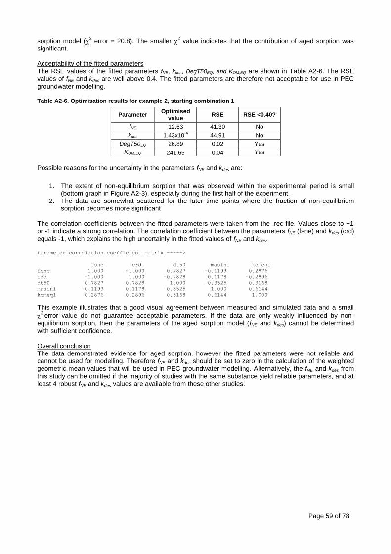
Page 59 of 78

sorption model (2 error = 20.8). The smaller

2 value indicates that the contribution of aged sorption was

significant. Acceptability of the fitted parameters The RSE values of the fitted parameters fNE, kdes, DegT50EQ, and KOM,EQ are shown in Table A2-6. The RSE values of fNE and kdes are well above 0.4. The fitted parameters are therefore not acceptable for use in PEC groundwater modelling. Table A2-6. Optimisation results for example 2, starting combination 1

Parameter Optimised

value RSE RSE <0.40?

fNE 12.63 41.30 No

kdes 1.43x10-4

44.91 No

DegT50EQ 26.89 0.02 Yes

KOM,EQ 241.65 0.04 Yes

Possible reasons for the uncertainty in the parameters fNE and kdes are:

1. The extent of non-equilibrium sorption that was observed within the experimental period is small (bottom graph in Figure A2-3), especially during the first half of the experiment.

2. The data are somewhat scattered for the later time points where the fraction of non-equilibrium sorption becomes more significant

The correlation coefficients between the fitted parameters were taken from the .rec file. Values close to +1 or -1 indicate a strong correlation. The correlation coefficient between the parameters fNE (fsne) and kdes (crd) equals -1, which explains the high uncertainly in the fitted values of fNE and kdes. Parameter correlation coefficient matrix ----->

fsne crd dt50 masini komeql

fsne 1.000 -1.000 0.7827 -0.1193 0.2876

crd -1.000 1.000 -0.7828 0.1178 -0.2896

dt50 0.7827 -0.7828 1.000 -0.3525 0.3168

masini -0.1193 0.1178 -0.3525 1.000 0.6144

komeql 0.2876 -0.2896 0.3168 0.6144 1.000

This example illustrates that a good visual agreement between measured and simulated data and a small

2 error value do not guarantee acceptable parameters. If the data are only weakly influenced by non-

equilibrium sorption, then the parameters of the aged sorption model (fNE and kdes) cannot be determined with sufficient confidence. Overall conclusion The data demonstrated evidence for aged sorption, however the fitted parameters were not reliable and cannot be used for modelling. Therefore fNE and kdes should be set to zero in the calculation of the weighted geometric mean values that will be used in PEC groundwater modelling. Alternatively, the fNE and kdes from this study can be omitted if the majority of studies with the same substance yield reliable parameters, and at least 4 robust fNE and kdes values are available from these other studies.

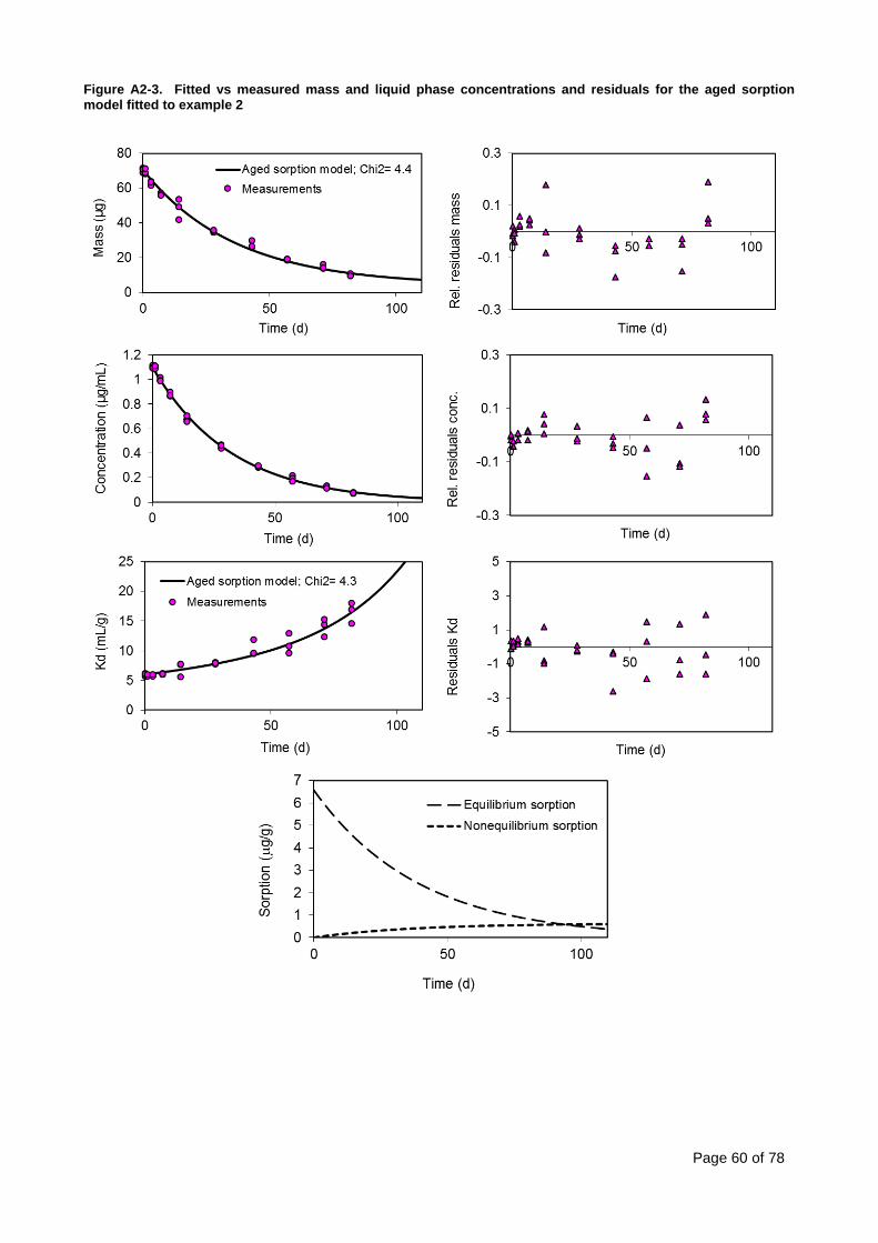
Page 60 of 78

Figure A2-3. Fitted vs measured mass and liquid phase concentrations and residuals for the aged sorption model fitted to example 2

Page 61 of 78

Figure A2-4. Fitted vs measured mass and liquid phase concentrations and residuals for the equilibrium sorption model fitted to example 2

Page 62 of 78

Appendix 3: Combining degradation and sorption data from Tier 1 and aged sorption studies – example cases

Two worked examples are presented in the EFSA Opinion

1 showing the combining of degradation and

sorption endpoints from Tier 1 with the new data from the aged sorption study, for deriving the final input parameters for groundwater modelling. Appendix B shows example ECPA-06, and Appendix C shows example ECPA-07. These are existing datasets provided by industry, and they demonstrate non-standard cases where there are multiple aged sorption studies (ECPA-06) or multiple measurements for the same soils (ECPA-07). Please refer to EFSA Opinion

1: https://doi.org/10.2903/j.efsa.2018.5382

and the following sections:

Appendix B.1.& C.1. Tier 1 assessment (without aged sorption) Appendix B.2.& C.2. Time-dependent sorption studies Appendix B.3.& C.3. Combination of degradation and sorption data from Tier 1 (without aged

sorption) and aged sorption studies 1 EFSA PPR Panel (2018) Scientific Opinion about the Guidance of the Chemical Regulation Directorate (UK) on how

aged sorption studies for pesticides should be conducted, analysed and used in regulatory assessments. EFSA Journal 2018;16(8):5382, 86 pp. https://doi.org/10.2903/j.efsa.2018.5382

Page 63 of 78

Appendix 4: Uncertainty review

The EFSA Scientific Committee (2015b) Draft Guidance on Uncertainty in EFSA Scientific Assessment provides specific guidance on the treatment of uncertainty when standardised assessment procedures are being developed. The first step is to identify the sources of uncertainties that affect the assessment for which the procedure is being developed. The main uncertainties in the aged sorption procedures identified by the authors of this report are listed in the Table and explained in the text below. Sources of uncertainty which are also applicable to the lower tier are not listed. In the Table below, most sources of uncertainty are classified as minor. The EFSA PPR panel (2018) noted that the wording ‘minor’ is optimistic in view of the potentially large effect of including aged sorption in the leaching assessment. There is indeed no doubt that the inclusion of aged sorption in PECGW calculations can significantly alter the result compared with lower tier modelling based on equilibrium sorption. However, this review does not investigate the effect of the uncertainty in aged sorption on the PECGW per se. Instead, it explores the effect of uncertainties in the assumptions and procedures that lead to a set of aged sorption model input parameters relative to the overall uncertainty in the PEC groundwater assessment. This overall uncertainty arises from e.g. the lower tier modelling concepts, tools and approaches, scenario assumptions and input parameters. Therefore, the categories ‘minor’ and ‘medium’ in the Table below indicate the magnitude of the relative contribution to the overall uncertainty and not an absolute effect.

Table A4-1. Identified sources of uncertainty and their estimated contribution to uncertainty in the risk assessment relative to the overall uncertainty in PEC groundwater calculations

Source of Uncertainty Estimated contribution to uncertainty in the risk assessment

Aged Sorption Concept and Model

1 The two-site model concept (versus multi-site) Minor

2 Sorption in the non-equilibrium domain is fully reversible; same rate constant for adsorption and desorption. First-order decline of mass in the equilibrium domain.

Minor

3 Non-equilibrium fraction not available for degradation Minor

4 Freundlich exponent for non-equilibrium sorption Unknown

5 Temperature dependency of sorption Minor

6 Moisture dependency of sorption Minor

7 Organic carbon is the main sorbent Minor

Methods

8 Extraction method and non-extractable residues Minor

9 Equilibration times Minor

10 Variability and reproducibility Minor

11 Sensitivity at low and high sorption Minor

12 Data quality and parameter reliability Minor

13 Inconsistencies between methods Minor

PEC calculations

14 Extrapolation from lab to field Minor

15 Averaging aged sorption parameters Medium

16 Combining lower-tier and higher-tier parameters Minor

17 Representative soils (minimum of 4 soils) Unknown

Description

1. Two-site sorption: Sorption is assumed to be instantaneous on part of the sorption domains, and rate-

limited on another part of sorption domains. In reality, in soil we expect a range of sorption domains with

various sorption rates. Sorption on both domains is described by a Freundlich isotherm. The two-site

model and Freundlich sorption model focus on describing the macroscopic sorption behaviour rather

than giving full insight into the underlying sorption mechanisms. Instantaneous sorption is used to

Page 64 of 78

quantify the very fast sorption that is typically measured in a standard batch sorption study. In the field, it

can take several days before the same level of sorption is reached, as there is not the same mixing with

solution. The amount of sorption in the field may therefore be somewhat overestimated by the model

during the first days. The choice of sorption model is expected to be a minor source of uncertainty, as

long as the two-site model is able to adequately describe the observed adsorption and desorption.

Uncertainties arise from extrapolation beyond the conditions in which the parameters are calibrated. For

example, if two-site model parameters are fitted on short-term behaviour (days), it may not give an

accurate description of long-term sorption (weeks/months).

2. Aged sorption is expected to be fully reversible. The model assumptions imply that pesticide residues are (slowly) released from the soil by desorption when the concentration in solution depletes. Desorption is described by the same rate constant as adsorption. The model does not explicitly account for a non-reversible fraction. The EFSA Panel (2018) does not share the opinion that aged sorption is expected to be fully reversible. However, the Panel emphasises that the proposed aged sorption model does implicitly account for the formation of irreversibly bound non-extractable residues in a sink term, which represents, apart from non-extractable residues, CO2, minor unidentified residues, as well as any metabolite, identified or not. Thus, non-extractable residues in the aged sorption model are treated as conforming to existing guidance on degradation kinetics (FOCUS, 2006). Therefore, the Panel does not consider the non-attainment of full reversibility of aged sorption to be a source of uncertainty. However, the formation of non-extractable residues does not necessarily meet the requirement of a first-order degradation process which is restricted to the equilibrium domain. The Panel considers that to be an additional source of uncertainty. Irreversible sorption would reduce the amount of pesticide available for leaching in the long term but is expected to have a minor effect on the total amount of leaching and the resulting PEC values.

3. Degradation of pesticide is assumed to occur in solution and in the equilibrium domain of the model and

is assumed to be first-order. No degradation is assumed to occur in the non-equilibrium domain. This is

in line with the theory that non-equilibrium sorption occurs by diffusion into denser soil particles or

aggregates, and that these areas would also be less accessible to micro-organisms. However, it is

uncertain where the boundary between available and non-available lies, and this may differ between

pesticides. The divide between degrading and non-degrading regions, and the slow transition between

them explains the bi-phasic degradation behaviour in many datasets. Over time, degradation slows down

as a smaller fraction of pesticide is available for degradation. As long as the model is able to describe

the bi-phasic decline of residues accurately during the model fitting, the uncertainty is expected to have a

minor effect on the leaching simulations.

4. Sorption at the equilibrium and non-equilibrium domain are described by the same Freundlich exponent

assuming the same nonlinearity for both domains. The exponent is derived in standard batch sorption

experiments performed on the same soil, representative for sorption at the equilibrium domains. It is

uncertain whether the exponent is representative for the non-equilibrium domains. The EFSA Panel

(2018) is of the opinion that any judgement of a possible impact on groundwater leaching assessment

caused by the violation of this assumption is premature without experimental or numerical (sensitivity

analysis with appropriate model) evidence. As the batch KOM and 1/n parameters used at the lower and

higher tier have a large effect on the PECGW, the EFSA Panel (2018) recommended to always apply the

quality checks outlined in EFSA (2017). Given the importance of the curvature of the Freundlich

isotherm, it is further recommended by the EFSA Panel (2018) to only accept Freundlich exponents from

studies of which sorption coefficients are accepted to be included in the further analysis. This is based

on the argument that if the sorption coefficient is considered not sufficiently reliable then the curvature

would be unreliable as well.

5. Temperature will have some effect on the sorption strength and rate, as it affects the solubility and

hydrophobicity of a substance, and affects reaction and diffusion rates. Within ambient temperatures, the

effect of temperature is expected to be small in comparison to for example the effect of temperature on

degradation rate. The effect of temperature on sorption is not considered in the modelling at lower or

higher tier.

6. Soil moisture content is assumed not to directly affect the sorption equilibrium constant KF. The same

sorption coefficient is assumed to be valid in relatively dry soils as in soil suspensions. It is uncertain

whether the soil moisture content may influence sorption in the non-equilibrium domain of the soil. If

aged sorption is due to diffusion into soil organic matter particles or aggregates through water-filled

pores, then the moisture content of the soil could influence the number of available diffusion pathways

and accessibility of the non-equilibrium domains. However, the drying out of the small pores into

aggregates would only occur in very dry conditions.

Page 65 of 78

7. Organic carbon is assumed to be the main sorbent for pesticides in soil. Unless a clear correlation is

found with other properties, sorption is expressed relative to the organic carbon content of the soils.

There is considerable variation in the KOM values at the lower tier, which illustrates the uncertainty

associated with this simplifying assumption. The same applies to the KOM,EQ values at the higher tier.

When aged sorption occurs, we assume that the non-equilibrium fraction of sorption also occurs on

organic carbon. In reality, part of sorption may occur on other substrates such as clay particles and

minerals, which may show different sorption behaviour (e.g. less reversible or less linear). For

substances that show a correlation of sorption with organic matter, it is assumed that organic matter is

also the main sorbent for the non-equilibrium fraction. As the same assumptions are applied for the

equilibrium fraction and the non-equilibrium fraction, the same uncertainties apply at the lower tier and

higher tier.

8. Non-extractable residue is not considered in the aged sorption model. This is justified by the assumption

that non-extractable residues are not available for leaching, and will never become available for

leaching. Any decline in extractable residue is interpreted as degradation and loss of pesticide mass.

The EFSA Statement emphasised the uncertainty caused by the solvent extraction method: The

extraction method needs to be strong enough to avoid overestimation of the non-extractable fraction. If

the extraction method is too weak and becomes less efficient over time due to stronger sorption, then

degradation would be overestimated and the increase in sorption over time would be underestimated.

Boesten (2016) showed that mild extraction methods are expected to give smaller fNE values (less

extracted residue means less aged sorption) and shorter DegT50 values (faster degradation). (The effect

on the fitted DegT50EQ was shown to be small as this parameter is partly compensated by the reduced

fNE.) Boesten then compared the PEC values; parameter values derived by harsh extraction resulted in

higher PEC values than those from mild extraction. At concentrations between 0.01 and 0.1 mg L-1

the

maximum difference in PEC values was a factor 2 (estimate based on the ‘best-guess’ scenario, which

was assuming 50% extraction efficiency for mild extraction). The effect on the risk assessment is

expected to be minor if EFSA’s recommendations are adhered to, and if sufficiently strong extraction

methods are used to extract the fraction that is reversibly sorbed and may become available for leaching

in the long term.

9. Equilibration time for the aqueous extraction (24 hours) was selected to reflect equilibration times

commonly used in standard batch sorption studies (see Defra, 2012, Chapter 2 for a more detailed

justification). Aged sorption is expressed as the increase in sorption beyond the 24-hour equilibration.

This cut-off point was chosen for practical reasons and to be consistent with existing procedures for

measuring sorption. We assume that spiking moist soil followed by 24-h equilibration with CaCl2 solution

gives the same amount of sorption as in a standard adsorption study (OECD 106) where the pesticide is

added to a suspension of soil in CaCl2 solution.

10. A standardised method is described in the guidance to minimise variability between studies and

laboratories, and to maximise reproducibility. Variability between laboratory results is expected to be no

different to other fate studies (OECD106 and 307).

11. Sorption measurements are more sensitive to experimental error in experiments with very little sorption

(very small change in concentration after sorption) or in experiments with a lot of sorption (final

concentration below limit of quantification). This uncertainty is the same as in standard sorption studies

when the direct method is applied, i.e. both the concentration in the equilibrium CaCl2 solution and the

adsorbed amount after extraction are measured, and is partly accounted for by optimising the soil-

solution ratio. The EFSA Panel (2018) notes that for mobile substances the soil-to-water ratio before the

extraction is more favourable in the aged sorption experiments. By applying the direct method, non-

extractable residues are treated in the same way as in an aged sorption study. Compared to the indirect

method, however, where the adsorbed amount of substance to the soil is calculated based on mass

considerations, the Panel assigns less uncertainty to aged sorption studies for mobile substances. The

indirect method is by experience still the most commonly used method in batch adsorption studies even

for mobile substances. The main source of error for mobile substances using the indirect method is that

the concentration in the input and in the equilibrium solution is almost equally large. The calculation of

the adsorbed amount of substance to the soil introduces a large uncertainty, because it is based on the

subtraction of two almost equally large concentration values. Calculating the adsorbed mass by

subtraction is not part of the procedure in aged sorption studies and therefore it is not a source of

uncertainty. For strongly sorbing pesticides, this uncertainty is not relevant as the groundwater

assessment will pass in any case. The resulting uncertainty for the leaching assessment is expected to

be minor.

Page 66 of 78

12. Uncertainties caused by data quality are accounted for by requirements regarding number of sampling

points, replicates, goodness of fit and parameter confidence intervals. A relative standard error smaller

than 40% allows some uncertainty regarding the aged-sorption parameter values. It was estimated that

approximately 10% of the model fits are accepted despite inaccurate parameters (deviation >25% of the

true value) due to variations in measurements and parameter uncertainty. Note that this estimate was

made using the procedures in the draft guidance (2012). Both accuracy and acceptance of the fitted

parameters will be different when using the new procedures. The effect on the groundwater assessment

is expected to be minor.

13. There are some differences between the methods for measuring sorption at the lower tier, and aged

sorption at the higher tier. At the lower tier sorption is measured in a soil suspension: The soil is pre-

equilibrated with pesticide-free solution to allow wetting of the soil before adding pesticide. This is

different from the aged-sorption study where pesticide is applied to moist soil, left for a short period, and

then equilibrated with aqueous solution. The order of adding pesticide and solution could affect the

sorption strength. Another difference is that at the lower tier, sorption is calculated based on the amount

of pesticide that was added (the nominal concentration) when the indirect method is used, and therefore

the amount of sorption could include non-extractable residues. In aged-sorption experiments, sorption is

calculated based on the extractable residue. The effect on the risk assessment is expected to be minor if

EFSA’s recommendations are adhered to, and if sufficiently strong extraction methods are used to

determine sorption.

14. Uncertainties are caused by extrapolation of laboratory observations to the fate of pesticides in the field.

Sorption and degradation experiments are performed on relatively small samples of soil, and pesticides

are mixed into the sieved soil rather than applied on top of the surface in the field. We assume that

sorption in shaken soil suspensions mimics the sorption that occurs in the field during transport down the

soil profile. Equally for aged sorption, we assume that aged sorption in relatively small mixed sieved soil

samples represents aged sorption in the field. Another limitation is that laboratory degradation and aged-

sorption experiments are performed over a limited period (generally up to 120 days to avoid a decline in

microbial activity). The observations are extrapolated over a longer period in the field during which

leaching may occur. Depending on the persistence of the pesticide this could be much longer than 120

days. The uncertainty is minimal when reliable parameters are derived from the laboratory study (which

is safeguarded by the RSE criteria). In order to obtain reliable parameters (and pass the RSE criteria),

the duration of the laboratory experiment needs to be sufficient to capture significant degradation, a

significant increase in sorption and plateauing of sorption. Then the risk of overestimating long-term

sorption beyond the duration of the experimental period is then expected to be small.

15. Averaging parameters: Representative substance parameters for input in the groundwater model are

derived by taking the arithmetic or geometric mean value from the available measurements for each

parameter (e.g. KOM, 1/n, DegT50). This averaging implies that each parameter represents an intrinsic

substance property that can be measured separately, and that there are no interactions between

parameters. Calculating an average PEC using average parameters gives different PEC values than

calculating the PEC with soil-specific combinations of parameters, and averaging the PEC values

afterwards. The effect of averaging the aged sorption parameters is expected to be minor in comparison

to the averaging of the main sorption and degradation parameters (KOM, 1/n and DegT50) as is common

practice at the lower-tier.

16. Combining lower and higher tier parameters: In principle, combining lower and higher tier degradation

and sorption data should reduce the uncertainty in the PECs as the dataset becomes larger, i.e. a larger

sample of the whole population of data is taken. But, as pointed out by the EFSA (2015) Statement,

there is some uncertainty as to how to combine lower-tier and higher-tier parameters for calculating PEC

in groundwater at the higher tier. The aged sorption parameters fNE and kdes are taken from aged sorption

studies, whilst the KOM,EQ is taken from standard batch sorption studies. Some uncertainty is caused by

combining parameters from different types of studies to describe the overall sorption, as aged sorption is

described relative to equilibrium sorption KOM,EQ, through the ratio fNE. The EFSA Panel (2018) points out

that the conversion of first-tier DegT50 values into DegT50EQ values introduces additional uncertainty.

The Panel considers that the best possible estimate of DegT50EQ is obtained with the recommendation

to use the refit to the residue data as the preferred option.

17. For assessments at the lower tier, sorption studies are performed on a minimum of 4 soils. Unless a

clear correlation is found with other properties, sorption is expressed relative to the organic carbon

content of the soils. The geometric mean KOC (or KOM) is used to estimate the 50th percentile KOC or KOM

for the population of agricultural soils in Europe. Given the large variability of KOC values between soils,

the limited number of soils introduces a high uncertainty. Similarly, aged sorption is measured on a

Page 67 of 78

minimum of 4 soils. There is very little knowledge on the variability for the aged sorption parameters fNE

and kdes between soils, and possible correlations with soil properties. Until this information becomes

available, it is not possible to assess the relative contribution of the variability in fNE and kdes to the overall

uncertainty and variability of the PECGW calculations. It should be kept in mind that the 1/n value is a

variable and sensitive parameter which causes variability in the risk assessment outcome in the

simulations with and without aged sorption. To minimise the uncertainty related to the variation between

soils, EFSA (2015) emphasises that the soils should be selected to represent contrasting soil properties.

Also they state that the majority of tested soils (with a minimum of four) should show aged sorption

before aged sorption can be considered in the risk assessment. The EFSA Panel (2018) emphasises

that additional uncertainty is introduced by the dependence of sorption and degradation parameters on

soil properties. It is well known that both the Freundlich distribution coefficient, KF (batch adsorption

experiments), and the degradation half-life, DegT50 (aerobic degradation experiments), may depend on

soil properties such as organic matter, pH and/or clay content. The same might apply for the factor

describing the ratio between the non-equilibrium and equilibrium Freundlich coefficients (fNE) and the

desorption rate coefficient (kdes). The Panel recommends that TDS is not applied to cases where there is

strong evidence for, for example, pH-dependent sorption, unless more evidence becomes available on

how to handle it.

A4.4 References

Boesten, J.J.T.I. (2016) Effect of harsh or mild extraction of soil on pesticide leaching to groundwater. Journal of Environmental Quality, May 2016. 9p. doi:10.2134/jeq2015.07.0363

EFSA (2015a). Statement on the FERA guidance proposal: ‘Guidance on how aged sorption studies for pesticides should be conducted, analysed and used in regulatory assessments’ (FERA, 2012). EFSA Journal 2015: 13(7):4175, 54 pp.

EFSA (2015b) Guidance on Uncertainty in EFSA Scientific Assessment. Revised Draft for Internal Testing. 274p. EFSA Scientific Committee. www.efsa.europa.eu

EFSA (2017). Technical report on the outcome of the pesticides peer review meeting on the OECD 106 evaluators checklist. EFSA supporting publication 2017:EN-1326, 17 pp.

EFSA (2018). Scientific Opinion about the Guidance of the Chemical Regulation Directorate (UK) on how aged sorption studies for pesticides should be conducted, analysed and used in regulatory assessments. EFSA Journal 2018; 16(8);5382, 86 pp.

FOCUS (2006). Guidance document on estimating persistence and degradation kinetics from environmental fate studies on pesticides in EU registration, report of the FOCUS work group on degradation kinetics, EC document reference Sanco/10058/2005 Version 2.0, 434 pp.

Page 68 of 78

Appendix 5: The Freundlich Exponent

Quality criteria for individual measurements

Given the high sensitivity of the leaching process on the Freundlich exponent, it is important to assess the reliability of reported values. In the absence of (i) detailed scientific analyses of the accuracy of the Freundlich exponent and (ii) tests of whether the exponent is a soil or a pesticide property, EFSA (2015) proposed a pragmatic procedure for the evaluation of measured 1/n values. However, EFSA have since released new guidance on evaluating OECD 106 studies; an OECD 106 evaluators’ checklist (EFSA, 2017), which supersedes these recommendations. The reader is therefore referred to the EFSA (2017) guidance document for suitable quality criteria for calculating a robust Freundlich exponent.

Averaging of the Freundlich exponent

The EFSA PPR panel (2015) recommends using the arithmetic mean of all reliable values. In view of the absence of a database of reliable 1/n measurements, the Panel recommends not setting strict limits for the 1/n values of sorption isotherms of a specific substance–soil combination. Therefore, values in the range of 0.6–1.2 are considered acceptable. However, if the arithmetic mean 1/n value exceeds 1.0, a value of 1.0 should be used because an exponent higher than 1.0 is considered physically unrealistic for the soil matrix. The EFSA PPR panel (2015) does not recommend using this restriction, 1/n ≤ 1, for individual sorption

isotherms because this would lead to a systematic bias (refer to Boesten et al. (2015) for details).

Current data requirements state a minimum of four values for sorption coefficients (three for relevant metabolites). If the OECD (2000) guideline was followed to obtain the sorption parameters, this would also lead to four (or three in the case of metabolites) Freundlich exponents. The draft guidance on aged sorption leads to a minimum of four Freundlich exponent values, subject to the quality criteria above, if the batch equilibrium method is used, implying that current data requirements would be met.

It has been common practice in groundwater leaching assessments to use a default value of 0.9 for the Freundlich exponent, because this is the average value of a large number of sorption studies (Calvet et al., 1980). This value may, however, not be conservative enough in a tiered approach because dedicated sorption experiments (parameter refinement) may result in 1/n values of > 0.9. A 1/n value of 1 would therefore be more appropriate in a tiered approach. The EFSA PPR panel (2015) recommends reconsidering the default value in view of the tiered approach introduced by FOCUS (FOCUS, 2009; updated by EC, 2014).

A5.5 References

Boesten JJTI, Van der Linden AMA, Beltman WHJ and Pol JW, 2015. Leaching of plant protection products and their transformation products. Proposals for improving the assessment of leaching to groundwater in the Netherlands – Version 2. Alterra Report 2264, Alterra, Wageningen, the Netherlands. Calvet R, Tercé M and Arvieu JC, 1980. Adsorption des pesticides par les sols et leurs constituents. III. Characteristiques générales de l’adsorption des pesticides. Annual Agronomy, 31, 239–257. EC (2014). Assessing Potential for Movement of Active Substances and their Metabolites to Ground Water in the EU. Report of the FOCUS Ground Water Work Group, EC Document Reference Sanco/13144/2010 version 3, 613 pp. EFSA PPR Panel (EFSA Panel on Plant Protection Products and their Residues), 2015. Statement on the FERA guidance proposal: ‘Guidance on how aged sorption studies for pesticides should be conducted, analysed and used in regulatory assessments’ (FERA, 2012). EFSA Journal 2015;13(7):4175, 54 pp. doi:10.2903/j.efsa.2015.4175 EFSA, 2017. Technical report on the outcome of the pesticides peer review meeting on the OECD 106 evaluators checklist. EFSA supporting publication 2017:EN-1326. 18 pp. doi:10.2903/sp.efsa.2017.EN-1326 FOCUS (Forum for the Coordination of Pesticide Fate Models and their Use), 2009. Assessing potential for movement of active substances and their metabolites to ground water in the EU. Report of the FOCUS Ground Water Work Group, EC Document Reference Sanco/13144/2010 version 1, 604 pp. OECD (Organisation for Economic Co-operation and Development), 2000. OECD guideline for the testing of chemicals. Adsorption–desorption using a batch equilibrium method. OECD Guideline 106, OECD, Paris.

Page 69 of 78

OECD (Organisation for Economic Co-operation and Development), 2002. OECD guideline for the testing of chemicals. Aerobic and anaerobic transformation in soil. OECD Guideline 307, OECD, Paris.

Page 70 of 78

Appendix 6: Research on the use of field data for aged sorption in regulatory leaching assessments

A6.1 Background

Recent research by Fera (Defra project PS2254) investigated the use of field data in relation to aged sorption (Defra 2015). This resulted in recommendations listed in the final chapters of the research report. The main findings are summarised here. The reader is referred to the full research report for details of the work underpinning the recommendations. It must be noted that the outcome of the research was not a guidance document.

Note that the EFSA Statement on aged sorption (EFSA, 2015) was released around the time of completion of project PS2254. The changes proposed in the Statement were not considered during the project, but they are implemented in this summary as far as possible. The EFSA Opinion on aged sorption (EFSA, 2018) recommends that field studies should not be used to derive aged sorption parameters until the guidance is further developed and tested with real world data.

A6.2 Methods

The aim of the research on field studies was to evaluate which types of field studies could be used to measure aged sorption, or how field data could be used in the leaching assessment in conjunction with aged sorption data derived from laboratory studies.

Four methods on aged sorption related to field studies were distinguished:

1. Field studies where aged sorption is measured by sampling the top soil at different time intervals

after application. Soil samples are extracted with CaCl2 solution to determine the readily available

pesticide, and extracted with solvents to determine the total extractable residue.

2. Aged sorption is measured in laboratory studies. Field data is used to determine a field DegT50EQ to

be used in conjunction with laboratory derived aged sorption parameters.

3. Profiles of the pesticide concentrations with depth are determined at different time intervals following

pesticide application in the field, and interpreted using aged sorption.

4. Pesticide concentrations are measured in percolate water at a certain depth, and interpreted using

aged sorption.

The first two methods were considered suitable for regulatory purposes, from a practical view point. Methods 3 and 4, and combinations thereof need very good characterisation of the soil properties and hydrology to allow reliable interpretation of the data, and are less likely to return reliable parameter values by model fitting. Therefore methods 3 and 4 were considered practically less suitable for regulatory use.

Field data was provided by industry to allow demonstration of the methods and to test some of the procedures. Four datasets were provided, each containing field data from several fields. One dataset was used for testing method 1 and three datasets followed method 2. Method 2 was further tested using artificially created data. The reader is referred to the research report for the results of this work (Defra, 2015). Recommendations on the procedures and the data requirements for Methods 1 and 2 are summarised below. Please note that method 1 is referred to as option 2 by the EFSA PPR panel (2018) and method 2 is referred to as option 1 because the panel preferred listing in order of increasing complexity.

A6.3 Recommendations for method 1

Method 1 aims at measuring aged sorption in field experiments. A field study is performed in a similar manner to field degradation studies. For the aged sorption measurements, samples are taken from the top soil (e.g. top 10 or 15cm) at certain time intervals and taken back to the laboratory for extraction and analysis. Similar to a laboratory study for measuring aged sorption, samples are extracted with CaCl2 solution to determine the pesticide concentration in solution, and extracted with solvent to determine the total extractable residue.

A leaching model, such as PEARL is used to interpret the sorption and degradation behaviour in the field. The model is coupled to an optimisation routine (e.g. PEST) to fit the pesticide degradation and aged sorption parameters. The optimisation procedure is described in detail in Chapter 5 of Defra (2015) for an example field study. The model used to derive the parameters does not have to be the same as the model that is later used for the PEC groundwater calculations.

The aim of the study is to derive aged sorption parameters. At the same time a field DegT50EQ is derived for use in the groundwater assessment. Therefore it is important that the study complies with the latest guidance on field DegT50 (EFSA, 2014). This includes procedures to avoid surface processes such as photolysis and volatilisation, and the design of field studies (Appendix A in EFSA, 2014). Samples taken before 10 mm

Page 71 of 78

rainfall must be eliminated in accordance with the EFSA guidance when no measures have been taken to minimise surface losses. Sufficient weather data and soil characterisation is needed for implementing the leaching model (more detail in Section 0).

Field studies show a larger amount of intrinsic variation between measurements. To ensure good data quality we therefore recommend to follow existing guidance for field degradation studies regarding number of replicates and sampling intervals.

Modelling procedure

The modelling procedure is similar to that described in the guidance for laboratory aged sorption studies, except that a leaching model is used to account for environmental factors that influence sorption and degradation. Otherwise the interpretation of the data is the same. Four degradation and aged sorption parameters (applied dose, DegT50EQ, fNE, kdes) are fitted to the measurements of mass and concentration. As described in the guidance, batch sorption experiments should be performed to derive the Freundlich exponent 1/n, preferably on soils from the same fields. The KOM,EQ value is fixed at the measured value on day 0 in the first instance, and the measurements on day 0 and 1 are included. This can be relaxed to improve the fit to the data.

The data requirements and acceptance criteria set out in the aged sorption guidance apply. A study would need to be performed on at least four soils with contrasting properties (laboratory or field studies). The decision tree in the guidance specifies that there should be evidence of aged sorption in the majority of tested soils, with a minimum of four soils showing evidence of aged sorption.

Sampling depth

EFSA guidance (2014) requires that the soil should be sampled up to 1 metre depth and divided into depth segments for analysis. If no pesticide is found in the next layer down, then subsequent layers do not need to be analysed. Field sites with excessive leaching are avoided, so losses below 1 metre depth are not expected.

For deriving field aged sorption parameters, only the top soil is extracted with CaCl2 solution, and only the measurements from the top layer are used in the modelling. The layer should not be too deep to minimise dilution with soil that does not contain pesticide but deep enough to capture the majority of the substance residue. Ideally for this method, the majority of the substance remains in the top 0-15 cm throughout the study period. This is inconvenient for pesticides that are tested for aged sorption, as these are likely to be the more mobile substances.

For deriving field DegT50 values (EFSA, 2014) it is important that all residue is captured by the sampling, as losses from leaching are not accounted for in the kinetic modelling. This is different in the method described here for aged sorption, as here we are using a leaching model to interpret the data. The model should in principle simulate the amount of leaching from the sampling layer, and therefore distinguish degradation from losses due to leaching. In reality the amount of leaching predicted by the model may cause uncertainty.

Defra (2015) suggested the following procedure: In accordance with EFSA (2014) soil sampling is performed up to 1 metre depth, and analysed for residues up to relevant depth. Samples from the top layer are used to measure aged sorption (extractions with CaCl2 solution and solvent). The residues in this and the subsequent layers are used to validate the DegT50. There are two options:

a. Use the extractions from the top layer to fit the model parameters for degradation and aged sorption

(Method 1). Then validate the fitted DegT50EQ by comparing the total residue up to 1-m depth

predicted by the model, against the measured sum of residues up to 1-m depth.

b. Use the extractions from the top layer to fit the model parameters for degradation and aged sorption

(Method 1). Do not use the fitted DegT50EQ, but only the fitted aged sorption parameters. Then re-fit

the field DegT50EQ on the total residues up to 1-m depth using Method 2.

Model fitting

Weighted fitting should be undertaken to conform with the aged sorption guidance for laboratory studies. This is to give equal weight to the measurements of mass and concentration, and to the smaller concentrations that affect the Kd at later time points.

Output from the leaching model cannot be compared to the field measurements directly: The leaching model calculates the concentration of the substance in soil solution, while the field measurements are concentrations in CaCl2 solution, after re-equilibration. Therefore the output from the leaching model has to be converted.

Defra (2015) created an algorithm in MatLab to calculate the concentration in CaCl2 after re-equilibration for each output line of PEARL. Output from PEARL are the variables ConSysEql (total concentration in the

Page 72 of 78

equilibrium domain) and ConSysNeq (non-equilibrium domain), both in kg a.s. m-3

soil, on each day. The concentration in CaCl

2 is calculated by iteratively solving the Freundlich equation, using the soil:solution ratio

during extraction, and the pesticide mass in the equilibrium domain. The algorithm is executed after each PEARL simulation, to write a new output file with the converted output data. PEST then compares the converted output against the measured data. Optimisation settings from the aged sorption guidance were used.

Evidence of aged sorption

The aged sorption guidance for laboratory studies tests for evidence of aged sorption by comparing the fit of the equilibrium sorption model and aged sorption model. The same principles can be applied to field data where total mass and aqueous extractable concentrations are measured.

Use in PECGW calculations

Aged sorption measurements should be available for four or more soils, and at least four should show evidence of aged sorption for the results to be used in PECGW calculations. The averaging of the parameters before use within the PECGW calculations should be consistent with the guidance for laboratory studies.

A6.4 Recommendations for Method 2

Method 2 is not aimed at measuring aged sorption in the field, but rather to derive a field DegT50EQ that can be used in combination with aged sorption parameters from the laboratory in PECGW calculations.

The aged sorption model assumes that degradation only takes place in the equilibrium domain. Therefore the DegT50EQ from the aged sorption model is conceptually different from a DegT50 that is derived from a standard degradation study. The DegT50 from field studies cannot be used directly in the groundwater assessment in combination with aged sorption. In these cases a field DegT50EQ needs to be derived. This is achieved by fitting the DegT50EQ to the field data, whilst accounting for aged sorption. During the model fitting, the aged sorption parameters are set to those derived in laboratory experiments.

Experimental requirements

The procedure is aimed at deriving a degradation endpoint for modelling, therefore study design, sampling and interpretation are covered by the EFSA guidance (2014). This includes procedures to avoid surface processes such as photolysis and volatilisation, and the design of field studies (Appendix A in EFSA, 2014).

EFSA (2014) guidance describes in Appendix A how field studies to determine DegT50 in the whole soil matrix should be designed. Recommendations include: at least three replicate subplots per field study, sampling at a minimum of eight time intervals, bulk samples from at least 10 samples (soil cores) per subplot on each sampling date, sampling to 1-m depth divided into depth segments. The guidance does not specify minimum requirements for legacy field studies. The suitability of legacy field data should therefore be judged on a case-by-case basis. Any study that is considered suitable for deriving a DegT50 in the soil matrix should in principle be suitable for deriving a DegT50EQ using method 2.

Method 2 involves the use of laboratory aged sorption data to derive a field DegT50EQ. The guidance for laboratory studies should be followed. The majority of tested soils (at least four) need to show evidence for aged sorption.

Where laboratory aged sorption studies have been undertaken with the soil from the field sites, it is recommended to use soil-specific parameters in the optimisation of each field DegT50EQ. In many cases, the aged sorption laboratory studies will have been conducted with other soils. Defra (2015) showed that the geometric mean of field DegT50EQ values derived for parameter combinations from individual aged sorption laboratory studies is similar to the DegT50EQ optimised using averaged parameters. Therefore, averaging of the aged sorption parameters from the laboratory prior to optimising the field DegT50EQ seems a good option. The averaging method (arithmetic mean, median or geometric mean) and recommendations for studies that show evidence for aged sorption but do not meet all the acceptance criteria should be consistent with the guidance on laboratory studies.

Data quality and handling

Measurements are taken from several soil layers up to 1 metre depth. The measured pesticide mass (e.g. in μg kg

-1) is converted to areic mass (e.g. kg m

-2) and then added up over all layers for each individual time

point. Samples before 10 mm rainfall need to be excluded according to EFSA (2014). FOCUS guidance on degradation kinetics (FOCUS, 2006, 2014) describes how to handle data below LOD and LOQ in laboratory studies. Defra (2015) made a proposal on how to handle measurements below LOD and LOQ when soil samples are taken and analysed separately for several soil layers, in line with the FOCUS guidance: ·

Page 73 of 78

On each sampling date, samples between LOQ and LOD are set to the measured values, or ½

(LOD+LOQ).

The mass is set to ½ LOD for the first depth with concentrations below LOD and omitted for all

deeper layers, unless the mass is >LOQ in any of the deeper layers. In this case, the mass is set to

½ LOD for all intermediate layers. This correction is carried out for each time point individually.

For the Day 0 data, it may not be appropriate to apply the above. In most cases the substance is

expected to be in the top layer only, and the residue in the next layer would be zero. Then there is no

reason to set the concentration in the next layer to ½ LOD. There may be exceptions, e.g. if the

incorporation depth is deeper than the top layer.

If the mass is <LOD for all depths at several consecutive time points, then it is set to ½ LOD in the

top layer on the first of these time points and omitted thereafter, unless a later sample is >LOQ. In

this case, the mass is set to ½ LOD for all intermediate time points.

As the LOD and LOQ are often expressed per soil mass (e.g. in μg kg-1

), these adjustments should be performed before converting the measurements into areic mass.

Model fitting

Model fitting should be undertaken with a pesticide leaching model that includes the two-site aged sorption model described in the guidance. The model used to derive the DegT50EQ does not have to be consistent with the model that is subsequently used for the PEC groundwater calculations.

The leaching model should be coupled with an optimisation tool, e.g. PEST. The use of tools such as ModelMaker that do not account for leaching is not recommended. Unweighted fitting is carried out in line with FOCUS (2006, 2014) using the total mass in the target soil layer (PEARL variable AmaSysTgt). The leaching model applies an internal correction on the degradation rate for actual soil temperature and moisture content during the simulations (rate-constant normalisation). For this purpose, the reference moisture is set to pF2, and the reference temperature to 20

oC, and default dependency factors are used

unless otherwise justified.

Latest EFSA recommendations to use time-step normalisation (EFSA, 2014) cannot be applied when aged sorption is concerned: The time-step normalisation method must not be used when fitting the aged sorption model, as this method would also affect the aged sorption rate constant kdes. The sorption rate constant is not expected to have the same temperature and moisture dependency as the degradation rate. The recommended method for deriving the DegT50EQ from field data is therefore by rate-constant normalisation.

Goodness of fit and parameter acceptability

For method 2, the recommendations by the FOCUS work group on degradation kinetics (FOCUS, 2006, 2014) apply: The goodness of fit should be assessed visually and statistically by calculating a χ

2- error using

the equations provided by FOCUS (2006, 2014).

Note that the t-test is not applicable when the DegT50EQ is fitted. The t-test is used to check that the degradation rate constant k is statistically different from zero, and therefore whether degradation occurs. This does not apply for half-lives, as a small DegT50EQ corresponds to very fast degradation.

Method 2 is performed to derive a DegT50EQ for use with aged sorption. It is not intended for testing if degradation in the field is significant or faster than in laboratory studies. We expect that these tests have already been performed on the data when the original field DegT50 for the whole soil matrix was derived from the data.

Use in PECGW calculations

Results from parameter optimisation should be available for at least four field studies. They can then be used in pesticide leaching models to calculate PECGW. Only degradation endpoints are derived in Method 2, and these should be used in the PECGW calculations in conjunction with the laboratory aged sorption data used in the optimisation of the DegT50EQ. The averaging of DegT50EQ from the various trials and their combination with lower tier data should be in line with the guidance for laboratory studies, and EFSA (2014).

A6.5 Soil properties and weather conditions

Leaching models such as FOCUS PEARL correct internally for the temperature and moisture dependency of degradation. For this reason, it is important that the model accurately describes the daily soil temperature and moisture content of the soil during the study period. To calculate the soil temperature and moisture content, the leaching model requires input of local weather data, a description of the soil profile and its hydrological parameters. Daily records of maximum, minimum and mean temperature (air and soil), total precipitation and potential evapotranspiration are recommended from five days prior to the first application of

Page 74 of 78

the pesticide through to the conclusion of the study (OECD 232, 2016). Alternatively, the daily potential evapotranspiration can be calculated from measurements of wind speed, relative humidity and solar radiation (Penman-Monteith), or simplifications thereof, e.g. using daily measurements of solar radiation (Makkink). Due to local variations in rainfall, it is advised to measure rainfall at a distance of less than 1 km from the field, or no more than 20 km for legacy studies (EFSA, 2014). The EFSA (2014) guidance recommends monitoring weather data for 5 days before the start of the study. However for the purpose of simulating the moisture content in the leaching model, it is beneficial to record weather data from at least a month before the start of the study.

A good description of the soil profile and soil properties is needed. The minimum requirements are sand, silt clay content and organic carbon or matter content for each soil horizon up to the maximum sampled depth. Bulk density and the hydraulic properties (van Genuchten parameters, hydraulic conductivity) can be estimated using pedotransfer functions (PTF). Several options can be tried and compared to find the PTF that best describes the moisture content of the soil, such as Hypres (Wösten et al., 1999) and Rosetta (Schaap, et al., 2001). In most cases, it will be appropriate to choose either Hypres or Rosetta, and to use alternative functions only if the fit is not satisfactory. To ensure that the fitted DegT50EQ is the value at reference conditions, it is important that the PTF describes the soil moisture content at field capacity (pF2). If needed, the water retention curve of the top soil can be calibrated against measured water retention data (water holding capacity at several tensions). The parameterisation of the model must be well documented.

To ensure that the model describes the soil moisture content sufficiently well, the model would ideally be validated against soil moisture measurements from the field, if available. The model should give a reasonable description of the soil moisture content in the top soil during the experimental period. Temporary deviations are fine, as long as the overall description is tolerable for calculating the moisture correction factor for degradation. The sensitivity of degradation for soil moisture is moderate, a 20% relative deviation in moisture content over the whole experiment would give 14-15% deviation in degradation rate. By comparison, this is slightly less than a deviation from the soil temperature by 2°C (Defra 2015).

A slower DegT50EQ will be derived when the model overestimates the temperature and/or soil moisture content in the field, therefore giving a conservative estimate in the groundwater assessment. If no satisfactory match can be achieved for the soil moisture content, then it would be an option to switch off the moisture correction in the model during the fitting of the DegT50EQ. This would give a worst-case DegT50EQ.

There are several methods for measuring the moisture content in the field. The most reliable method is probably gravimetrically by taking regular samples from the top soil and drying these in the oven to determine weight loss. In new studies, the moisture content can easily be determined for the top soil samples taken on the sampling dates. Sometimes the timing of these samples may be far apart and then it could be helpful to take moisture samples more regularly. Other methods involve moisture probes such as TDR probes. In legacy studies these measurements are not always available. Sometimes the moisture content is reported for subsamples, for correcting the weight of soil in the sample, but these moisture contents are not necessarily representative of the fresh field samples. EFSA (2014) states that soil moisture data are not readily available for many field soil dissipation experiments. In those cases they advise that average daily soil moisture contents may be estimated with predictive models. This implies that EFSA does not expect a validation against soil moisture measurements for legacy studies.

It would be useful if criteria for the simulation of water contents for new studies could be developed. These should consider if and how the modelled data need to be checked against measurements. If a comparison is considered necessary, then it is important to specify at which depths and at which temporal resolution the moisture should be recorded and modelled, how the goodness of fit should be assessed visually and statistically, and which deviations can be tolerated. The magnitude, timing and duration of the deviations needs to be considered and whether there are consistent over- or underestimations or random deviations. A good match is most important during the time where most of the degradation occurs. The general accuracy in soil moisture measurements should be taken into account. The sensitivity of the DegT50EQ for deviations in moisture and its implications for PECGW calculations should be considered.

OECD 232 (2016) and EFSA (2014) require measurements of the soil temperature during the field study. Best practice according to EFSA is for the daily average soil temperature to be determined at a depth of 10 cm. Models may be used to estimate the average daily soil temperatures in cases where soil temperature data is not available (EFSA, 2014). Defra (2015) recommended comparing the modelled soil temperature data with the measured data when available, and discuss the implications for the derived DegT50EQ. The reader is also referred to the discussion by EFSA (2010) Chapter 2.3 and 2.4 regarding uncertainties around the temperature and moisture correction of DegT50 in the whole soil matrix. The comments made are equally valid for DegT50EQ.

Page 75 of 78

A6.6 References

Defra (2015). Use of field data to generate aged sorption parameters for regulatory leaching

assessments. Report to Defra for project PS2254. The Food and Environment Research

Agency.

EFSA (2010). Guidance for evaluating laboratory and field dissipation studies to obtain DegT50

values of plant protection products in soil. EFSA Journal 8(12): 1936, 67 pp.

EFSA (2014). EFSA Guidance document for evaluating laboratory and field dissipation studies to

obtain DegT50 values of active substances of plant protection products and

transformation products of these active substances in soil. EFSA Journal 12(5): 3662, 37

pp.

EFSA (2015). Statement on the FERA guidance proposal: ‘Guidance on how aged sorption studies

for pesticides should be conducted, analysed and used in regulatory assessments’

(FERA, 2012). EFSA Journal 13(7):4175, 54 pp.

FOCUS (2014). Generic Guidance for Estimating Persistence and Degradation Kinetics from

Environmental Fate Studies in Pesticides in EU Registration (version 1.1) EC Document

Reference Sanco/10058/2005 version 2.0, 434 pp.

OECD (2016) Guidance Document for Conducting Pesticide Terrestrial Field Dissipation Studies.

Series on Testing and Assessment No. 232, Series on Pesticides No. 82: OECD

Environment, Health and Safety Publications ENV/JM/MONO(2016)6, 87p.

Schaap, M.G.; Leij, F.J. and van Genuchten, M.Th. (2001). Rosetta: a computer program for

estimating soil hydraulic parameters with hierarchical pedotransfer functions. Journal of

Hydrology 251 (3–4):163-176.

Wösten, J.H.M.; Lilly, A.; Nemes, A.; Le Bas, C. (1999). Development and use of a database of

hydraulic properties of European soils. Geoderma 90: 169-185.

Page 76 of 78

Appendix 7: Research on the use of metabolite data to generate aged sorption parameters for regulatory leaching assessments

A7.1 Background

Recent research by Fera (Defra project PS2254) investigated the use of the guidance on aged sorption for metabolites that are either formed from parent compounds or directly applied (Defra, 2015). This resulted in recommendations listed in the final chapters of the two research reports. The main findings are summarised here. The reader is referred to the full research report for details of the work underpinning the recommendations. It must be noted that the outcome of the research was not a guidance document.

Note that the EFSA Statement on aged sorption (EFSA, 2015) was released around the time of completion of project PS2254. The changes proposed in the Statement were not considered during the project, but they are implemented in this summary as far as possible.

Two types of studies can be distinguished for aged sorption of metabolites: metabolite-dosed studies and parent-dosed studies. In parent-dosed studies, the formation, degradation and aged sorption of the metabolite are investigated simultaneously, as well as the degradation of the parent substance. Modelling these processes involves a large number of parameters to be derived by model fitting. This can cause additional uncertainty in the fitted aged sorption parameters for the metabolite.

It was therefore recommended that aged sorption parameters for metabolites should be derived from metabolite-dosed studies. Parent-applied studies are only recommended for metabolites formed from fast-degrading parent substances. The EFSA Opinion on aged sorption (EFSA, 2018) recommends deriving aged sorption parameters for metabolites only from metabolite-dosed studies. In this case the guidance for the parent compound also applies to the metabolite.

A7.2 Metabolite-dosed studies

In metabolite-dosed studies, the metabolite is applied to the soil directly. The study is used to derive the aged sorption parameters for the metabolite, including the equilibrium KOM,EQ and the DegT50EQ. The Freundlich sorption exponent that is needed for the model fitting should be derived from standard batch sorption experiments (OECD 106). As normal for metabolite-applied studies, the formation fraction of the metabolite cannot be derived during the aged-sorption study. For the groundwater simulations, the formation fraction will need to be estimated from other parent dosed studies or set to a conservative value of 1.

Equivalence of metabolite-dosed and parent-dosed studies

It is assumed that metabolites behave the same whether gradually formed over time or whether added all at once, as in a metabolite-applied study. One could argue that for a metabolite formed from a parent, the metabolite is already in the aqueous phase at the time of formation, whereas in the metabolite dosed study, a proportion could be present as a solid depending on its solubility. This could suggest that degradation rates might be slower where metabolites are dosed directly if they have to first dissolve into the aqueous phase in order for degradation and sorption to start occurring. But during work for Defra (2015) data that confirm this were not identified. The assumption that there is no difference between parent dosed and metabolite dosed studies is consistent with the approach for lower tier DegT50 where metabolite endpoints from both study types are routinely accepted and included in tier 1 assessments. In theory, the aged sorption model is valid for both situations, and the same rate constant and formation fraction applies in both cases. The model calculates aged sorption dynamically by gradient-driven flow between compartments, therefore mathematically the model is valid independent of whether the metabolite is added to the compartment at once or gradually.

There are a few assumptions in the model that could influence the behaviour of metabolites. One important assumption in the conceptual model is that degradation only occurs in the equilibrium phase, and therefore the metabolites are formed in the equilibrium phase. If a substance behaves differently, for example if parent degrades in the non-equilibrium phase and its metabolite is formed in the non-equilibrium phase, then the current model for aged sorption is no longer valid. In that case the model could derive different parameters from a metabolite-applied or parent-applied study. However, there is no evidence that would suggest that the current conceptual model is invalid. Defra (2015) proposes that, unless there is evidence for a metabolite that it behaves differently when dosed directly, it can be assumed that a metabolite-dosed study is valid for measuring aged sorption.

A7.3 Parent-dosed studies

The proposed procedure is to perform an aged sorption study with dosed parent as described in the guidance. To derive aged sorption of the metabolite, one would measure the concentration of metabolite in

Page 77 of 78

CaCl2 extract. For modelling, the following data are needed for each time point: (1) the total extractable amount of parent substance in the soil sample, (2) the total extractable amount of metabolite in the soil sample (μg) and (3) metabolite concentration in CaCl2 solution (μg/mL).

Data requirements and handling

The guidance on data requirements and data handling applies which includes the need for batch sorption experiments (OECD 106) to determine the Freundlich exponent 1/n, and the instructions on number of datapoints , replicates and data above LOQ. The comments made on legacy studies also apply to metabolites.

Model fitting

The models described in the parent guidance cannot be directly used for metabolites in parent dosed studies. The models need adjusting to describe the formation of the metabolite from the parent before describing aged sorption of the metabolite. The adjustment is shown for ModelMaker in Figure 2 of Defra (2015).

Stepwise model fitting is used, starting by fitting the initial mass (Mp,ini) and degradation (DegT50) for the parent compound to the measurements of the parent residues using first-order kinetics in the first instance. During the second step, these parent parameters are fixed to the fitted values. Then the parameters for the metabolite are fitted (formation fraction, DegT50EQ, KOM,EQ, fNE, kdes) to the metabolite measurements. Weighted fitting using the reciprocal value of each measurement is used to give equal importance to measurements of mass and concentration, and to give equal importance to small concentrations.

The EFSA Statement (EFSA, 2015) recommends to fit the aged sorption model with KOM,EQ fixed at the value calculated from the measurements on Day 0. This is not possible for the metabolite in parent-applied studies, as the metabolite concentration is zero on Day 0. The metabolite KOM,EQ must be fitted.

If the parent compound shows a bi-phasic decline, then the model should be modified in accordance with FOCUS guidance. If both parent and metabolite are subject to aged sorption, then the model could be adjusted to describe aged sorption of the parent and the metabolite, and fitted stepwise first to derive the aged sorption parameters of the parent, and secondly to derive the aged sorption parameters for the metabolite. The additional measurements (mass and concentration measurements for both parent and metabolite) justify the fitting of the larger number of model parameters without compromising the reliability of the parameters. It is possible that the fitted parameters for either the parent or the metabolite do not meet the acceptance criteria of the aged sorption guidance. If the fit for the parent does not meet the acceptance criteria, then a conservative approach needs to be followed for the parent. But the only requirement for fitting the metabolite parameters is that the model gives an adequate description of the decline of the parent mass. As long as the decline in the parent mass is described well, the parent model can be used.

Acceptance criteria

In accordance with the guidance on aged sorption, the model needs to give a visually and statistically acceptable fit to the data. In addition the data must show evidence of aged sorption to justify the use of aged sorption in the FOCUS groundwater simulations. Evidence for aged sorption is tested by comparing the model fit of the aged sorption model with an equilibrium model. The applicability of the test for metabolites was demonstrated by Defra (2015). The assessment was done for artificial datasets with varying amounts of aged sorption. The test positively confirmed the occurrence of aged sorption for all tested datasets. Passing the test confirms that aged sorption is relevant for the dataset in question

The reliability of the fitted parameters is assessed from the confidence interval (or standard deviation) that is given by the optimisation software for each of the fitted parameters. The confidence interval is used to calculate the Relative Standard Error (RSE) for each parameter. For parent or metabolite compounds that

are directly applied to the soil samples, the acceptance level set by the guidance is RSE 0.4. The suitability of the RSE criterion was tested by Defra (2015). Based on the results, it is proposed that aged sorption parameters should only be derived from parent-applied studies with fast degrading parent compounds. Depending on the required conservatism, it needs to be decided where to set the limit between a fast degrading and slow degrading parent substance. Defra (2015) only tested parent half-lives of 50 or 10 days, the limit could be somewhere in between these values.

Although it is not recommended to derive aged sorption parameters for metabolites from parent-applied studies (unless a fast degrading parent compound), modelling the data from parent-applied studies can possibly be used to test for evidence for aged sorption (by comparing model fits as described in Section 4.6 of the guidance).

Page 78 of 78

A7.4 References

Defra (2015). Use of metabolite data to generate aged sorption parameters for regulatory leaching assessments. Report to Defra for project PS2254. The Food and Environment Research Agency.

EFSA (2015). Statement on the FERA guidance proposal: ‘Guidance on how aged sorption studies for pesticides should be conducted, analysed and used in regulatory assessments’ (FERA, 2012). EFSA Journal 2015:13(7):4175, 54 pp.

FOCUS (2014) Generic guidance for estimating persistence and degradation kinetics from environmental fate studies on pesticides in EU registration. Version 1.1, 18

th December 2014.