EUROPEAN COMMISSION HEALTH & CONSUMER PROTECTION DIRECTORATE-GENERAL Directorate E – Food Safety: plant health, animal health and welfare, international questions E1 – Plant health

Sanco/1090/2000 – rev.1

June 2003

GUIDANCE DOCUMENT FOR ENVIRONMENTAL RISK AS-SESSMENTS OF ACTIVE SUBSTANCES USED ON RICE IN

THE EU FOR ANNEX I INCLUSION

Final Report of the Working Group "MED-RICE" prepared for the European Commission1 in the framework of Council Directive 91/414/EEC.

This document has been conceived as a working document of the Commission Services, which was elaborated in co-operation with the Member States. It does not intend to produce legally binding effects and by its nature does not prejudice any measure taken by a Member State within the implementation prerogatives under Annex II, III and VI of Commission Directive 91/414/EEC, nor any case law developed with regard to this provision. This document also does not preclude the possibility that the European Court of Justice may give one or another provi-sion direct effect in Member States.

1 Contributing authors: A.-B. Delmas (chair), F. Alfarroba, D. Arnold, S. Cervelli, B. Erzgräber, P. Gaillardon, D. Gomez de Barreda Castillo, R. Jackson, J. Linders (secretary), S. Loutseti, W.-M. Maier.

2

Working Group Membership

F. Alfarroba DGPC, Portugal

D. Arnold Aventis, UK, until 1 October 2000

S. Cervelli Institute of Soil Chemistry, Italy

A.-B. Delmas INRA, France (chairman)

B. Erzgräber Aventis, Germany, later BASF, Germany

P. Gaillardon INRA, France

D. Gomez de Barreda Castillo IVIA, Spain

R. Jackson Dow Agrosciences, UK

J. Linders RIVM-CSR, The Netherlands (secretariat)

S. Loutseti Ministry of Agriculture, Greece, until 1 January 2003

W.-M. Maier European Commission, Belgium

R. Maycock Dow Agrosciences, UK (replacing R. Jackson)

J.-L. Alonso Prados INIA, Spain (replacing D. Gomez de Barreda Castillo)

Preferred citation: MED-Rice (2003). Guidance Document for Environmental Risk Assessments of Active Sub-stances used on Rice in the EU for Annex I Inclusion. Document prepared by Working Group on MED-Rice, EU Document Reference SANCO/1090/2000 – rev.1, Brussels, June 2003, 108 pp.

3

TABLE OF CONTENTS Page EXECUTIVE SUMMARY........................................................................................................ 4 1. INTRODUCTION............................................................................................................ 10 2. RICE CROPPING IN EUROPE ...................................................................................... 11

2.1 General ......................................................................................................................... 11 2.2 France ........................................................................................................................... 14 2.3 Greece........................................................................................................................... 19 2.4 Italy............................................................................................................................... 22 2.5 Portugal ........................................................................................................................ 28 2.6 Spain............................................................................................................................. 33 2.7 Overview ...................................................................................................................... 42

3. SCENARIO DEFINITION .............................................................................................. 43 4. DATA REQUIREMENTS............................................................................................... 44

4.1 Fate and Behaviour....................................................................................................... 44 4.1.1 Introduction .......................................................................................................... 44 4.1.2 Fate and Behaviour Studies – Annex II of Directive 91/414/EEC ...................... 44

4.2 Ecotoxicology............................................................................................................... 48 4.2.1 Introduction .......................................................................................................... 48 4.2.2 Ecotoxicological Studies – Annex II of Directive 91/414/EEC........................... 48 4.2.3 Ecotoxicological Studies – Annex III of Directive 91/414/EEC ......................... 50 4.2.4 Risk Assessment................................................................................................... 50

5. PEC CALCULATIONS................................................................................................... 52 5.1 Definitions.................................................................................................................... 52 5.2 PEC in surface water, including Sediment................................................................... 56

5.2.1 Introduction – Tiered Approach........................................................................... 56 5.2.2 Methods proposed – Step 1a, 1b and 1c............................................................... 58 5.2.3 Proposed model in Step 2..................................................................................... 63 5.2.4 Available models – Step 2 and 3.......................................................................... 63

5.3 Groundwater................................................................................................................. 65 5.3.1 Introduction – Tiered Approach........................................................................... 65 5.3.2 Methods proposed – Step 1 .................................................................................. 67 5.3.3 Proposed model in Step 2..................................................................................... 70 5.3.4 Available methods – Step 2 and 3........................................................................ 71

5.4 Soil ............................................................................................................................... 72 5.4.1. Introduction – Tiered Approach........................................................................... 72 5.4.2. Methods proposed – Step 1a and 1b..................................................................... 74 5.4.3. Step 1a, application to flooded soil ...................................................................... 74 5.4.4. Step 1b, application to drained field..................................................................... 75 5.4.5. Step 2, modelling.................................................................................................. 75 5.4.6. Step 3, site-specific situation................................................................................ 75

6. CONCLUSIONS.............................................................................................................. 77 7. RECOMMENDATIONS ................................................................................................. 79 REFERENCES......................................................................................................................... 80 APPENDICES.......................................................................................................................... 83

A. Example Input Data for EXCEL sheets ....................................................................... 84 B. EXCEL sheet for PEC in Surface Water excluding Sediment..................................... 87 C. EXCEL sheet for PEC in Soil and Sediment ............................................................... 96 D. EXCEL sheet for PEC in Groundwater: .................................................................... 105

4

EXECUTIVE SUMMARY The need for a guidance document on rice When Annex VI to Council Directive 91/414/EEC was adopted (Directive 97/57/EC2), the Council and the Commission recognised that due to particular conditions associated to rice cultivation the specific criteria and principles referred to in Annex VI were inappropriate. At this occasion the Commission committed to identify any specific data requirements and de-velop criteria for environmental risk assessment and decision-making which specifically ad-dress the use of plant protection products in rice cultivation. The current document intends to fulfil this obligation. The approach taken An expert group was appointed with the task to develop a common system for the risk as-sessment of PPPs in rice, at least at the lower Steps of the risk assessment especially intended for the inclusion of a substance in Annex I of the Directive and to report the results in a Guid-ance Document for data requirements and risk assessment in rice cultures to be adopted by the Standing Committee on Plant Health. The group made an inventory of the rice agricultural practices in the 5 South-European mem-ber states, France, Greece, Italy, Portugal and Spain, considering the main similarities and dif-ferences. From this comparison two European standard scenarios were abstracted, which model two different and representative situations in particular with respect to contamination of surface waters and leaching of substances applied to the paddy field. The following table ES.1 shows the basic parameters of the two scenarios defined by the working group. Table ES.1. Proposal for scenario definition Characteristic Scenario proposal 1 Scenario proposal 2 Soils: * texture Clayey Sandy * % clay 30 5 * % o.m. (% o.c.) 3 (1.8) 1.5 (0.9) * pH 8 6 Water level 10 cm 10 cm Water velocity: * outflow 0.5 l/s/ha 0.5 l/s/ha * field 1.8 l/s/ha 2.8 l/s/ha Flooding conditions May – August May – August Time of closure of field 5 days 5 days Depth of drainage channel 1 m 1 m Crop rotation No No Infiltration (leakage) rate 1 mm/d 10 mm/d Evapotranspiration rate 10 mm/d 10 mm/d Usage of outflow water No No Temperature (ºC) 20 20 Conditions in soil Aerobic Aerobic

2 OJ L265 27 September 1997, p87

5

Additional data requirements for rice cropping A revision of data requirements as defined in Annex II and III of the Directive 91/414/EEC was undertaken to conclude on their appropriateness to rice culture. The workgroup concluded that regarding the requirements for Fate and Behaviour in the envi-ronment some adaptations were regarded as necessary considering the agricultural peculiari-ties of this culture. The main changes were related to the evaluation of the route and rate of degradation. It was concluded that a flooded soil degradation study would better address the degradation of active substances under paddy field conditions. The suitable protocol devel-oped by SETAC3 and OECD4 307 for aerobic and anaerobic transformation in soil is then recommended. Following this protocol a typical soil study representative of rice growing should be used. Additionally, a small-scale or full-scale outdoor dissipation study with radio-labelled material may give useful information for certain compounds (e.g. where photolysis may be important). For the ecotoxicology data requirements since the application of plant protection products in rice culture may coincide with the breeding season of birds it is possible that birds or nesting sites be exposed to those products during the application. Also, rice paddies are often located in or in the vicinity of Natural Reserves with great importance as habitats for waterfowl and migratory bird species. Nevertheless it was concluded that current guidance was considered sufficient for Annex I inclusion and that additional testing was not required. Taking into consideration the scenario definition (table ES. 1) Step 1 PEC5 calculations meth-ods for surface water, groundwater and soil were developed for plant protection products ap-plied in rice crops, following as much as possible the current approaches used at the EU level. It should be noted, however, that the approach followed to calculate PEC in groundwater at Step 1 of the risk assessment differs from the procedure adopted for plant protection products used in other field crops. Proposal for a standard risk assessment The working group developed a tiered approach in three steps, starting from a relatively sim-ple calculation of the Predicted Environmental Concentrations (PECs) up to a sophisticated approach using complex modelling and monitoring at the highest level. The group focused on three environmental compartments, surface water, including sediment, groundwater and soil. For these three compartments a method was developed to estimate the actual PEC values and the Time Weighted Average (TWA) concentrations over relevant time periods. These PECs are then used in the risk assessment for relevant non-target organisms. At this stage, the working group limited itself to develop a standard Step 1 assessment, as ad-vanced mathematical modelling tool are not yet sufficiently validated to be used in a regula-tory context. The generalised tiered approach is shown in the following scheme, Figure ES.1. The way the scheme is elaborated for the different compartments is shown in the respective paragraphs.

3 SETAC: Society for Environmental Toxicology and Chemistry 4 OECD: Organisation for Economic Co-operation and Development 5 PEC: Predicted Environmental Concentration

6

Figure ES.1. Generalised Tiered Approach

Remark: it should be kept in mind that the schemes are just for illustrative purposes and do not represent the full extent of assessment that may be carried out. Estimation of PECs in rice paddy fields The working group developed a method to estimate the PEC in different environmental com-partments. These compartments are surface water, including sediment, groundwater and soil. A distinction is made between the actual PEC estimates and the TWA for different time points or periods. For further details reference is made to the text of the document (Chapter 5).

1. Surface water, including sediment (both degradation and sorption considered): water phase (outflow):

yes

no

yes

no

Step 1Loading based on total dose

Step 2Model calculations for paddy rice scenario

using advanced mathematical modelsno further

work

Step 3

Refined exposure modelling incl. site specificconsiderations and/or geographical/statistical

approaches

Usesafe?

Usesafe?

7

)1/())()(()( , dilutionclosepwdilutionclosedriftswclosesw facttPECfacttPECtPEC ++⋅= (1)

and sediment phase:

sedseddilution

sorbedwaterclosepwclosedriftsedclosesed BDdepthfact

FdepthtPECtPECtPEC

⋅⋅

⋅⋅+=

)()()( , (2)

For the time weighted average concentrations the following equations are used:

water phase:

sw

DTTinitialsw

sw DTTePEC

TTWAsw

50/)2ln()1(

)(50/)2ln(

,

⋅−⋅

=⋅−

(3)

and sediment phase:

sed

DTTinitialsed

sed DTTeTPEC

TTWAsed

50/)2ln()(

)(50/2ln

,

⋅

⋅=

⋅−

. (4)

2. Groundwater (both degradation and sorption considered):

For the estimation of the concentration in groundwater the following equations have been de-rived for the concentration in groundwater:

leakageM

tPEC leakpgw ⋅

⋅== >

365100

)365( )1000( (5).

3. Soil (both degradation and sorption considered):

For soil the following equations are proposed for the calculation of the PEC in soil as concen-tration and time weighted average:

soilDTtinitialsoilsoil ePECtPEC 50/2ln

,)( ⋅−⋅= (6)

soil

DTtinitialsoil

soil DTtePEC

tTWAsoil

50/)2ln()1(

)(50/)2ln(

,

⋅−⋅

=⋅−

(7)

Use of the guidance The proposed methodology gives notifiers and authorities the information on the data re-quirements needed to be considered for fate and behaviour and ecotoxicology as well as a standard tool how to calculate the appropriate PECs for the purpose of review for inclusion in Annex I of Council Directive 91/414/EEC. To ensure consistent and convenient application of the scheme, easy to use spreadsheets are attached to this document to estimate PEC values.

8

Conclusions The following conclusions may be drawn from the work presented here. 1) The workgroup has completed its given task to develop procedures that can be used for

making decisions for the Annex I inclusion of plant protection products used in rice. In order to fulfil this task, the present document was compiled, covering the following as-pects: - agronomic and environmental conditions in rice growing regions in the EU - review and adjustment of the data requirements regarding fate and behaviour in the

environment and ecotoxicology - review of appropriate modelling tools for the estimation of exposure to the environ-

ment by plant protection products used in rice crops. 2) The group has identified the following main areas, which need consideration within the

scope of this guidance document: soil, groundwater, surface water and sediment in the paddy and in the drainage canals. In addition, the ecological function of aquatic organisms within the paddy field should be considered at Member State level if appropriate.

3) The review of the cropping conditions in the five Southern EU countries concerned by this

crop has revealed many similarities. The two different standard scenarios proposed repre-sent dominant situations occurring in the MS of concern and offers limited but relevant differences, one based on vulnerable conditions for leaching and the other being more suited to estimate risks in surface waters.

4) Limited changes are proposed in Annex II of Directive 91/414/EEC with regard to the

evaluation of the fate and behaviour of plant protection products in the environment. These affect mainly the test system to be used for investigation of route and rate of degra-dation in soil. It was concluded that an aerobic flooded soil study would be more appro-priate and should replace the normal aerobic soil degradation study. Also, a decision scheme is proposed with regard to the possible necessity of higher tier (e.g. small-scale or full-scale outdoor dissipation) studies. For registration at the national level, relevant regu-latory authority judgement would be required.

5) The major contribution is concerning Annex III. Regarding PEC calculations for soil,

ground waters and surface waters, relevant models for paddy rice conditions have been se-lected on a step 1 purpose for soil and ground waters and up to a step 2 approach for sur-face waters. The specific case of outflow canals has been particularly taken in account. Simple new models or existing more sophisticated ones as RICEWQ have been selected.

6) Environmental fate and behaviour and ecotoxicology requirements have been reviewed

and amended as necessary to account for the specific requirements of rice culture. 7) For ecotoxicological data requirements the workgroup has concluded that current guid-

ance on how to perform the risk assessment for non-target species is acceptable. Aquatic organisms in the rice paddy itself do not require the same level of protection as those in the non-target water bodies adjacent to the fields. However, other species that may use the treated rice paddies as a feeding ground (e.g. birds and mammals) do require the normal level of protection. If specific concerns are identified at national level higher tier studies should be considered on a case by case basis.

9

8) Currently adopted methods for PEC calculations for surface water, soil, and groundwater were found to be not fully appropriate for paddy field conditions. Therefore, a stepwise approach has been developed for the estimation of PEC in these compartments after appli-cation of plant protection products in rice. Simple calculation methods for the step 1 as-sessment were developed, which follow partly the current approach for surface water and soil, but deviate from the currently adopted methods for the assessment of leaching to groundwater.

9) Based on current practice separate steps are defined for taking into account degradation

and sorption of the active substance under consideration. 10) Relevant simulation models for paddy rice conditions have been reviewed and proposals

are made for higher tier exposure assessment. Among the readily available simulation models, RICEWQ was considered to be appropriate for the assessment of exposure in sur-face waters. Further research would be needed to fully evaluate the applicability of RI-CEWQ or other models. The model RICEWQ is proposed to be used in connection with RIVWQ model to estimate the PECs in surface waters. RICEMOD may be an appropriate model if more information on it becomes available.

11) Currently, regulatory models to predict groundwater contamination are limited in their

ability to simulate the flooded conditions of a paddy rice field. Thus no model can be rec-ommended at this stage for such simulations and further research is required. If models recommended by the FOCUS6 leaching modelling workgroup are used the limitations of those need to be kept in mind in the evaluation process. Nevertheless, to take into account the specific hydrological aspects of the rice culture it is currently considered that the best approximations can be achieved with Richards’ equation based models.

12) The development of specific leaching models for rice paddies will give the possibility for

refining PECsoil estimates. 13) In summary, keeping the presentation of the Directive, a document simple to read and to

consult in order to prepare a dossier for EU registration purposes was produced. The method followed has been fully presented for clarity of the options retained in this inte-grated approach. This choice intends also to help both Companies and Authorities if a sci-entific difficulty arises in the preparation of a dossier to evaluate how far the problem to solve deviates from the proposals of the Working Group.

14) The work of the Group is considered a good compromise between an evident lack of sci-

entific information regarding the requirements in the domain of environment and an ur-gent need of guidance for registration purpose at EU level. The present guidance docu-ment is aimed at providing a tool for the regulatory decisions needed. Present proposals could be improved in the near future for EU registration and more urgently if used also for national registration purposes.

6 FOCUS: FOrum for the Co-ordination of pesticide fate models and their USe

10

1. INTRODUCTION When the Annex VI to Council Directive 91/414/EEC – The Uniform Principles - was adopted, the European Council (in Document 10171/97, ADD1, Agrileg 163 dated from 22 August 1997) among others made the following statement:

“…The Council and the Commission note that particular conditions obtain in rice cultivation. This means that certain specific criteria are inappropriate for evaluation purposes, particularly in the context of point 2.5.2.2. for the exposure of aquatic organisms in rice field waters. …”

In order to develop the necessary Guidance to Member States and notifiers as to how the risk to non-target organisms should be addressed in rice cultivation, the Standing Committee for Plant Health has charged a small expert group with the development of a proposal. In addi-tion, the Steering Committee of FOCUS decided that flooded systems as for paddy-rice crop-ping were out of the scope of FOCUS.

The task given to the expert group was:

• the development of a common system for the risk assessment of PPPs in rice, at least at the lower Steps of the risk assessment especially intended for the inclusion of a sub-stance in Annex I of the Directive and

• to report the results in a Guidance Document for data requirements and risk assess-ment in rice cultures to be adopted by the Standing Committee on Plant Health.

It is not the task of the working group and it is also outside the scope of the present Guidance document, to develop scenarios for national authorisations or make any other prejudice in this context. However, it is hoped that the present document may serve as a useful source of in-formation also for these purposes.

In Chapter 2 the document describes current rice cropping practices in the relevant Member States, i.e. France, Greece, Italy, Portugal and Spain. From this survey, two representative scenarios are distilled and defined in Chapter 3. Chapter 4 outlines data requirements on fate and behaviour and ecotoxicology, which were found to be particularly relevant for rice cul-tures. Deviations, additions and points of special emphasis as compared to Annex II and III requirements of the Directive are indicated. In Chapter 5 guidance is provided for the estab-lishment of the Predicted Environmental Concentrations (PECs) in the relevant environmental compartments, namely surface water including sediment, groundwater and soil. Current de-velopments in the scientific community are described in Chapter 6, which would be of use in near future to improve the methodologies available today and proposed at this stage.

Overall conclusions are summarised in Chapter 7. Chapter 8 outlines the recommendations of the workgroup for further activities and projects, which should be initiated to develop refined tools for Step III risk assessments.

In the Annexes the scenarios and proposed methods are formalised in easy to use spread-sheets, which can serve for the Step I and Step II calculation of PECs for soil, surface water, sediment and groundwater.

11

2. RICE CROPPING IN EUROPE 2.1 General In the year 2000, the rice growing area within the European Union has been about 400000 ha. As shown in Figures 2.1.1 and 2.1.2 the most important countries of rice cultivation are Italy (221000 ha), Spain (111000 ha), Portugal (22000 ha), Greece (17000 ha), and France (19000 ha). Spain and Greece are the countries where rice surface has recorded the largest variation in the last ten years, with an increase of about 24 and 68 %, respectively. Rice in Europe is grown under a Mediterranean climate characterised by warm, dry, clear days, and a long growing season favourable to high photosynthetic rates and high rice yields. Compared to tropical and subtropical rice-growing areas, the climate is cool, but warm sum-mer nights during panicle development, when pollen formation

Figure 2.1.1. Main areas of rice cultivation in Europe. takes place, helps to avoid cold-induced floret sterility. Low relative humidity throughout the growing season reduces the development, severity, and importance of rice diseases. However, cool weather and strong winds during stand establishment may cause partial stand loss and seedling drift. Rice is grown mostly on fine-textured, poorly drained soils with impervious hardpans or clay pans. These soils are principally in three textural classes: clays, silty clays, and silty clay loams ranging from 10 to 45 percent clay. A few of the soils are loam in the surface horizon but are underlain with hardpans. These soils are well suited to rice production, since their low water permeability enhances water use efficiency. Most of the irrigation water for European rice comes from rivers (Po river in Italy, Ebro river in Spain, Rhone river in France, Tejo, Sado and Mondego rivers in Portugal, etc.) and lakes. It is estimated that less than 5 percent

12

of rice irrigation water is pumped from wells in areas where surface water is not available, or as a supplement to surface supplies. The high cost of pumping well water prevents its wide-spread use in rice production. Surface water and most groundwater are of very good quality for rice irrigation.

Figure 2.1.2. Rice surface in European countries in 2000. In all European countries rice is commonly cultivated with a permanent flood with short peri-ods during which soil is dried up to favour rice rooting (in the early stages) or weed control treatments. The conventional irrigation system is also known as a "flow-through" system, be-cause water is usually supplied in a series from the topmost to the bottom most basin and is regulated by floodgates by means of removable boards. This irrigation system shows the following advantages:

• low cost, • easy to install, maintain, and remove , • good performance with irregular slopes;

and the following drawbacks: • risk of pollution of public waters by chemicals, • lack of independent control of each basin.

Average yield has been approximately 6.6 tons ha-1, but in many farms it is possible to record average productions of about 7.5 tons ha-1. Improved varieties and cultural practices have contributed significantly to yield increases since the 1960s. The most important of these practices include:

Italy53%

Spain27%

Greece7%

France5%

Portugal8%

Surface 2000(ha x 10 00)

1990- 2000var ia tion

I ta ly

Spain

Por tuga l

Gr ee ce

France

221

111

22

27

20

+ 3 .7 %

+ 24 .7 %

- 6 .4 %

+ 68 .7 %

+ 7.8 %

13

• more efficient nitrogen management, • effective herbicides for the control of broadleaf and grass weeds, • precision land levelling with laser-directed equipment widely adopted, • development of semi-dwarf rice varieties introduced in the 1980s.

14

2.2 France Rice culture accounts for about 20000 ha in France, mostly in Camargue (Figure 2.2.1). This region is situated in southern France, inside the Rhone delta, near the Mediterranean Sea. It is a flat area with a mean altitude of about 5 m. It is characterised by the presence of shallow salty ground water at a depth ranging from 0.6 to 2 m in the south part and > 2 m in the north part of the delta. Because rice culture needs high fresh water supply and allows downward water movement in soil in summer, it plays a key role in preventing soil from salting. Paddy fields are partly included in the Natural Park of Camargue, which is a protected area.

Figure 2.2.1. Distribution of paddy fields in Camargue (yellow). Two other minor areas of rice cultivation are shown in boxes. (from CFR, Arles)

Weather is characterised by hot and dry summer, and cool and wet winter. At Mejanes (near Arles), the mean monthly temperature ranges from 6.6 °C (January) to 22.9 °C (July). Rainfall mainly occurs in autumn and in winter but annual rainfall shows high variability: 406 – 1009 mm, mean 622 mm (Table 2.2.1). At Arles annual rainfall is in the range 361-1037 mm (mean is 762 mm) and at Sainte Marie de la Mer (seaside) the mean annual rainfall is 629 mm.

15

Table 2.2.1. Weather data recorded at Mejanes (years 1989-2000). Month E.T.1) Rainfall Temperature ( °C) (mm) (mm) Mean Max. Min. January 20.5 59.5 6.6 11.2 3.2 February 37.8 27.5 8.0 13.1 4.0 March 84.0 26.4 11.0 16.7 6.3 April 104.1 69.5 12.9 17.8 8.4 May 135.0 33.0 17.5 22.2 13.1 June 149.3 34.4 20.3 25.4 15.4 July 167.7 16.4 22.9 28.5 17.8 August 136.9 47.4 22.7 28.8 17.7 September 87.3 90.8 18.7 24.8 13.9 October 49.4 104.5 15.0 20.3 11.1 November 25.2 65.0 9.8 14.4 6.3 December 17.7 47.3 7.0 11.4 3.8 Total or mean 1015 622 14.4 19.5 10.1

1) E.T. = evapotranspiration Soils are not homogeneous. Distribution of soil characteristics of paddy fields in Camargue is shown in Table 2.2.2. Data are derived from soil analysis provided by CFR (Centre Français du Riz) based in Arles. Sand is generally < 40 % (median 16 %). Clay content typically ranges from 10 to 40 % (median 25 %), silt from 40 to 70 % (median 55 %) and organic mat-ter from 1 to 4 % (median 2.5 %) even though larger ranges are observed. It should be noticed that rice straw is usually burnt because of slow decay in soil. Soils are alkaline with pH in the range 7.6 - 8.9 but most soils have a pH between 8.0 and 8.5. In accordance with these data, two major soil types can be distinguished by expert judgement. One type corresponds to clay rich soils with low permeability and the other type to coarser soils with higher permeability. Characteristics of a representative soil from each type are given in Table 2.2.3. Table 2.2.2. Distribution of soil characteristics of paddy fields in Camargue.

Clay (< 2 µm) Silt (2-50 µm) Sand (> 50 µm) Organic Matter Content Freq.* Content Freq.* Content Freq.* Content Freq.*

0 – 10 % 12 30 – 40 % 14 < 10 % 77 < 1 % 7 10 – 20 % 56 40 – 50 % 42 10 – 20 % 41 1 – 2 % 55 20 – 30 % 67 50 – 60 % 75 20 – 30 % 38 2 – 3 % 88 30 – 40 % 46 60 – 70 % 61 30 – 40 % 23 3 – 4 % 36 40 – 50 % 19 - - > 40 % 24 4 – 5 % 7

> 50 % 6 - - - - 5 – 6 % 6 - - - - - - > 6 % 5

17 / 25 / 34 %** 48 / 55 / 62 %** 6 / 16 / 29 %** 1.8 / 2.5 / 3.1 %** * Freq.: frequency (number of soils in each class of content) ** 25th percentile / median / 75th percentile

16

Table 2.2.3. Characteristics of the representative soils (2 major types).

Soil type (location) Silty clay loam (Boulevard) Silt loam (Romieu) Clay (%) 35 21 Silt (2-50 µm) (%) 61 (2 – 20 µm, 44 %) 51 (2 – 20 µm, 33 %) Sand (%) 4 28 OM (%) 2.50 1.85 pH 8.0 8.1

The size of paddy fields is typically 400 – 600 m x 50 m (2 – 3 ha). Fresh water comes from the Rhone River and is supplied to paddy fields by means of canals. Output water is drained into ditches (1.5 – 2.5 m depth) along paddy fields and flows (or is pumped) toward the Medi-terranean Sea or large ponds (Vaccarès). Ditches account for a significant proportion of total surface (roughly 15 – 20 %). Crop rotation (2 years rice and 3 years wheat) is a common practice in the major part of Camargue but permanent rice crop occurs in the south, near the Mediterranean Sea. Rice seeds are sown in April-May (from the end of April to the beginning of May) on dry soil be-fore flooding or in water of flooded soil. Before sowing, particular practices including flood-ing and soil tillage or herbicide application can be involved to control wild rice (red rice). Herbicides are the primary plant protection products applied to rice crop for weed control (es-pecially Echinochloa crus-galli, Cyperus and broad leaf weeds). Treatments include both early (May) and late (June) applications to flooded soil and to wet soil after emptying paddy field depending on herbicide and a maximum of 3 treatments are applied each year. No fungi-cides are used to control diseases and insecticides are occasionally used (one treatment in summer if needed). Seed treatment is in progress. Methods of application involve aerial treatments at about 1 m above paddy fields and terrestrial treatments by means of sprayer equipped with nozzles and mounted on tractor. Usually, water depth in paddy field is about 10 cm. It can be lower after sowing and higher (up to about 20 cm) at late growth stage in Au-gust. Fields are closed for 5-7 days after herbicide application to flooded soil and then a slow stream is allowed. More detailed information about rice cropping may be obtained from CFR (Centre Français du Riz). A typical water balance has been proposed by Heurteaux (1996). Water supply is in the range 20000 to 30000 m3 ha-1. For a 4 month flooded period, the mean input water flux would be 2 – 3 L ha-1 s-1. Water losses (Figure 2.2.2) may occur by evapotranspiration, lateral infiltration to ditch, infiltration to ground water, emptying paddy field and water stream in paddy field (outflow).

17

Figure 2.2.2. Water losses from paddy fields (adapted from Heurteaux, 1996). Evapotranspiration (ET) is the major process and accounts for about 10000 m3 ha-1. Infiltra-tion to ditch amounts to about 5000 m3 ha-1 and emptying to about 3000 m3 ha-1. Stream (out-flow) is estimated to be in the range 0 – 8000 m3 ha-1 (mean 4000 m3 ha-1). For a 4 month pe-riod, the mean output water flux would be 0.4 L ha-1 s-1. Infiltration to ground water is esti-mated to be about 5000 m3 ha-1. For a 4 month period, the mean infiltration would correspond to 4 mm d-1. This value could be lower for clay rich soils and higher for sandy soil. Assuming that infiltration to ditch does not occur in sandy soils and that the corresponding water moves to ground water, infiltration to ground water would not exceed 8 mm d-1. Water balance data are summarised in Table 2.2.4. Table 2.2.4: Typical water balance for rice culture

Water volume Water flux* Water supply 20000 – 30000 m3 ha-1 1.9 – 2.9 L ha-1 s-1 Water losses Evapotranspiration 10000 m3 ha-1 - Infiltration (ditch) 5000 m3 ha-1 - Emptying 3000 m3 ha-1 - Stream** (outflow) 0 – 8000 m3 ha-1 0.38 L ha-1 s-1 Infiltration (ground water)

5000 m3 ha-1 0.48 L ha-1 s-1 (4.2 mm d-1)

* mean value for a 4 month flooded period ** water flux estimated for the mean volume (4000 m3 ha-1) Rice cropping in France is summarised in Table 2.2.5.

Evapotranspiration

Ditch

Emptying Stream

Infiltration to ground water

Lateral infiltration

Paddy field

18

Table 2.2.5: Overview of rice cropping strategies in France.

Characteristic France Soils: * texture Silt loam/ Silty clay loam * % o.m. 1 – 4 * pH 8.0 * % clay 10 – 40 Drainage system Yes Water level Max. 20 cm,

average 10 cm Water velocity: * drainage (outflow field) 0.4 l/s/ha * field (inflow field) 2 – 3 l/s/ha Flooding conditions May – Aug Time of closure of field 7 days Depth of outflow channel 1.5 – 2.5 m Crop rotation Yes Infiltration (leakage) rate Max < 8 mm/d, Mean 4

mm/d Usage of outflow water No Aeroplane application Yes Irrigation system No Temperature (ºC) > 14 Aerobic/anaerobic conditions at interface Aerobic

19

2.3 Greece The main area for rice cropping is Northern Greece with some areas in the central part of the country (17000 ha). Rice fields are situated on either side of riverbanks or their Delta’s. There are no reports of them being next to lakes.

Figure 2.3.1. Greece and rice cropping areas. The soils are mainly silty-loam soils. Sowing of rice seeds takes place in May at low water levels, while weed control applying herbicides is done at normal water levels. The herbicides are used generally 20 – 30 days after sowing and 2 – 3 applications are usual with an interval of 5 days. The rice fields are flooded during June, July and August with a water supplementa-tion every five days. The main loss of water is due to evapo-transpiration and infiltration. September is the rice maturation time and the fields are kept dry. Complete irrigation and drainage systems exist in 75% of the rice fields with some excep-tions. The water level is between 5 – 10 cm during cultivation period. This could be main-tained at 2 – 3 cm in order to avoid the appearance of certain species of weeds (weed control) or pests (it could happen the first 45 days after sowing). The water after the 3-leaf growth stage remains in the rice field and supplementation of water takes place every 5 days. Due to reasons of water economy (water shortage) complete renewal of water is avoided. In cases of high salinity in soils it is important to renew the water every week.

20

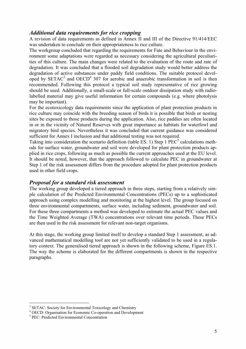
The rice field is filled with water (flooded) before sowing and remains like this until the 20th of September. The water is drained from the fields 10 – 15 days before harvesting. Harvesting begins on the 15th of September and finishes at the end of October. Crop rotation is applied every 3 – 4 years. Usual crops are maize and alfalfa. This is not the case for rice fields with soils of high salinity (about 20%). The drained water is not used due to problems of increased salinity in soils and negative ef-fects to the rice production. Aeroplanes are not used for pesticide or fertiliser application. The water temperature should be at least 12 °C in order to have successful sowing. Nevertheless temperatures in the range of 25 – 29 °C are considered better. For the normal growth of the rice plants the air temperatures should be between 25 and 33 °C. Table 2.3.1: Overview of rice cropping strategies in Greece.

Characteristic Greece Soils: * texture Silty loam * % o.m. 1.8 – 2.0 * pH 7.4 – 8.0 * % clay 20 Drainage system Yes (75%) Water level 2 – 10 cm Water velocity: * drainage (outflow field) 0.5 l/s/ha * field (inflow field) 4 l/s/ha Flooding conditions May – Sept Time of closure of field 2-5 days Depth of drainage channels 1.5 – 2.0 m Crop rotation Yes (80%) Infiltration (leakage) rate 5 – 10 mm/d Usage of outflow water No Aeroplane application No Irrigation system Yes (75%) Temperature (ºC) > 12 Aerobic/anaerobic conditions at interface Aerobic

The majority of soil types used in rice fields has high salinity and is for this reason unsuitable for the cultivation of other crops. Before their use as rice fields they were mainly grassland. During 20 – 30 years of use as rice fields they have been improved and crop rotation (3 years rice cultivation and 1-year maize cultivation) management has been established. The sowing of rice and water management depend on the degree of soil salinity. In these cases sowing is performed while the water level is at least 4 – 5 cm deep. Flooding with water is also very important for the successful leaching and removal of the different salts present in the soil. The water drained form the rice fields in the Districts of Thessaloniki, Pieria, Pelis and Imathias (Macedonia – North of Greece) ends up in the Thermaikos Bay. Some of the drained water can re-enter the irrigation canals in other areas further up north, were the problem of salinity does not exist. This applies also to the Districts of Serres (ending up to Strimonikos Bay) and the District of Fthiotidos (ending up in Maliakos Bay). Water management has contributed, however, to about 50% reduction in the amount of plant protection products used. Until the year 1990 rice fields were flooded up to 10 – 20 cm at the

21

first stages of plant development. In some areas due to levelling limitations the water level could have reached up to 35 cm. Today water levels are controlled and maintained at 4 – 5 cm via the use of modern laser techniques. Also water management contributed to better pest and weed control (10 years ago due to high levels of water present in rice fields, there were in-creased outbreaks of insect and crustacean attacks – but no weeds were present). However, while the use of insecticides has decreased, the use of herbicides has increased. Contamination of surface waters with plant protection products was detected, especially with the herbicide Molinate and some organophosphate insecticides. In Greece a monitoring study has been carried out in the most important rice area, the Axios River (15000 ha rice cropped) basin since 1992 (INTERREG PROGRAMMES 1& 2 Ministry of Agriculture). Both Moli-nate and Propanil were among the pesticides most frequently found in the main drainage channel systems of the basin with concentrations ranging from 0.03 µg/l (min) to 6.82 µg/l (max.) and 0.17 µg/l (min) to 1.11 µg/l (max.) respectively. Many species such as earthworms, snakes, frogs, spiders, etc. inhabit the rice fields, while a variety of beneficial arthropods i.e. Coccinella etc. are present. Many reeds are situated next to the rice fields, which could be useful in some cases (wind brakes). Pelicans, storks, swal-lows, hawks and many migratory birds find food in the rice fields and shelter to the areas next to them. The ecological characteristics (from target and non-target organisms) and risk as-sessment for the use of plant protection products in the representative areas need to be further investigated. There are no data as to the effects on birds and fish species present in the rivers and lakes from the application of insecticides and herbicides in rice fields. In some cases negative effects were suggested but no severe cases of intoxication have been reported. During September and October there is an influx of fish in the rice fields, coming from the water in the canals, and also human bird-hunting activities have increased.

22

2.4 Italy Rice is cultivated on about 221000 hectares (2000), mainly in the northern part of Italy (Piemonte, Lombardia, Veneto and Emilia Romagna) and Sardegna (Figure 2.4.1). The cultivated area in northern Italy may in its turn be divided in a northern (mean area of rice fields 2 – 3 ha) and a southern part (mean area of rice fields about 10 ha).

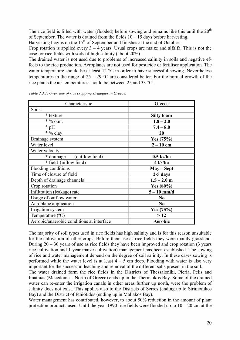
Figure 2.4.1. Area of rice cultivation in different Italian regions (2000). About 85% of the Italian north-western area is cultivated with japonica varieties under flood-ing conditions. Since the beginning of the 1960s, rice has been mechanically direct-seeded. Now, 85% of the production area is broadcast-planted in flooded fields. The remaining area is row-planted in dry soil and flooded, starting from the beginning of crop tilling. In these condi-tions, rice has no competitive growth advantage over weeds that can compete with the crop from the beginning of stand establishment. Main rainfalls are concentrated during the first stages of the crop (April – June) and during harvesting period (Figure 2.4.2). Average temperatures range from 10 – 12 °C occurring dur-ing rice germination, to 20 – 25 °C, recorded during crop flowering. Rice planted in dry soil is commonly managed as a dry crop until the crop reaches 3 – 4 leaf stage; after this period rice is flooded as in the conventional system with continuous flooding.

111,351 ha

94,183 ha

3,683 ha

8,192 ha

347 ha

3,271 ha

511 ha

Tot 221,538 ha

soil area cropped to rice

PiemonteLombardia

Veneto

Toscana

Sardegna

Calabria

Emilia Romagna

23

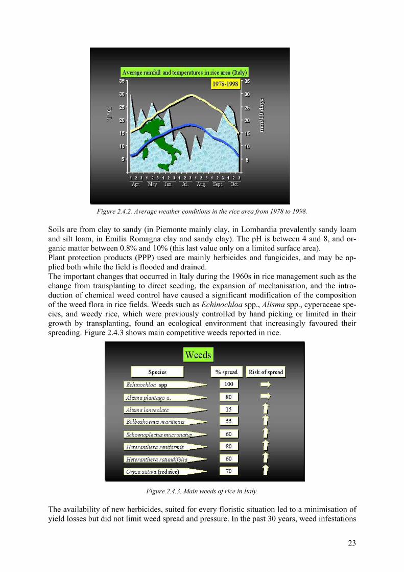
Figure 2.4.2. Average weather conditions in the rice area from 1978 to 1998. Soils are from clay to sandy (in Piemonte mainly clay, in Lombardia prevalently sandy loam and silt loam, in Emilia Romagna clay and sandy clay). The pH is between 4 and 8, and or-ganic matter between 0.8% and 10% (this last value only on a limited surface area). Plant protection products (PPP) used are mainly herbicides and fungicides, and may be ap-plied both while the field is flooded and drained. The important changes that occurred in Italy during the 1960s in rice management such as the change from transplanting to direct seeding, the expansion of mechanisation, and the intro-duction of chemical weed control have caused a significant modification of the composition of the weed flora in rice fields. Weeds such as Echinochloa spp., Alisma spp., cyperaceae spe-cies, and weedy rice, which were previously controlled by hand picking or limited in their growth by transplanting, found an ecological environment that increasingly favoured their spreading. Figure 2.4.3 shows main competitive weeds reported in rice.

Figure 2.4.3. Main weeds of rice in Italy. The availability of new herbicides, suited for every floristic situation led to a minimisation of yield losses but did not limit weed spread and pressure. In the past 30 years, weed infestations

24

have become more severe because of the spread of existing weeds and the introduction of ex-otic plants. The area of infestation of Heteranthera species, which were sporadically reported for the first time only at end of the 1960s, increased by 80% in about 30 years, and, in spite of the good performance of some herbicides, a further expansion of infestation is foreseen. A similar situation can be observed with weedy rice, a plant with negligible importance until rice was transplanted and which is now present in 75% of the rice fields. Weeds cause the greatest damage to rice in Italy. Without weed control, crop losses were estimated, at a yield level of 7 to 8 t ha-1, as high as 92% (Ferrero and Tabacchi, 2000; Ferrero, Tabacchi and Vi-dotto, 1999). PPPs can be applied in paddy fields in several different ways:

• directly on dry soil, • directly on wet soil (1 cm water), • directly on water (7 – 10 cm), • first on dry soil and then on water, • in post emergence on water (at least 10 cm), • in post emergence on water (1 cm).

The whole Italian rice surface is commonly sprayed with 1-3 treatments of herbicides chosen among 27 active ingredients at present registered for rice application. It is estimated that the quantity of the herbicide active ingredients applied yearly ranges between 0.35 and 13 kg ha-1 according to the type of infestation and the herbicide utilised. The highest amount of herbi-cides refers to the application of Dalapon, a herbicide utilised for red rice control. In the last years it is possible to record a trend towards early-stage treatments and applications of low rate herbicides with less dangerous ecotoxicological behaviour. Figure 2.4.4 reports a general scheme for the rice treatments with PPP and, according to the growing stage, other important agronomic operations.

Figure 2.4.4. Calendar of common rice operations. The water regime is mainly characterised by:

25

• the depth of the water on average is about 10 cm, and decreases during the season (4 months in a year, usually from May to September) by evapotranspiration,

• alternation of submersion (10 or 1 cm water) and dry periods during the growing sea-son,

• complex hydrologic regime, set through networks of drainage canals and ditches, • slow water flow directly from rice fields and little canals into receiving canals and riv-

ers. Three irrigation systems are currently used:

• separate fields, feeding and discharging occurring through different canals, • irrigation and drain canals are the same, • water is supplied in a series from the topmost to the bottom most basin and is regu-

lated by floodgates by means of removable boards (flow-through). Figure 2.4.5 reports the water balance determined in a large rice area near Vercelli (Piemonte, northern Italy).

Figure 2.4.5. Water balance of the selected area of about 693 km2 near Vercelli, Piemonte, northern

Italy (from Greppi et al., 1998), where the time and boundary conditions are:

time interval = 1 March - 30 September (214 days) area cropped to rice = 693 km2

and the input and output data are: inflow field (in + rain) = 250.8 x 103 m3 h-1 = 3.61 m3 ha-1 h-1 = 1.010 l sec-1 ha-1 drainage (outflow field) = 38.1 x 103 m3 h-1 = 0.55 m3 ha-1 h-1 = 0.153 l sec-1 ha-1.

Plane application of PPPs is inhibited in Italy. No crop rotation is generally used and the fields are not flooded during winter.

1-2 m

out

38.1 x 10 3 m 3 h-1 (195.7 x 10 6 m3)

in

211.6 x 10 3 m 3 h-1

(1.087 x 10 9 m3)

rain39.2 x 10 3 m 3 h-1 (201.5 x 10 6 m3)

by GREPPI (1998)

0.25-0.46 mm h -1

(888-1638 x 10 6 m3)

26

Figure 2.4.6 shows a picture of a portion area cropped to rice near Vercelli.

Figure 2.4.6. Typical area cropped to rice near Vercelli, Piemonte, northern Italy. In Table 2.4.1 an overview of rice cropping strategies in Italy is given.

27

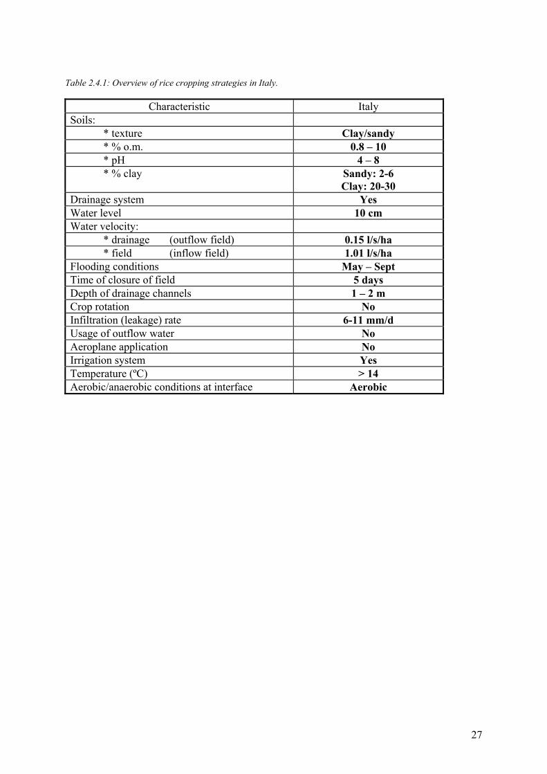
Table 2.4.1: Overview of rice cropping strategies in Italy.

Characteristic Italy Soils: * texture Clay/sandy * % o.m. 0.8 – 10 * pH 4 – 8 * % clay Sandy: 2-6

Clay: 20-30 Drainage system Yes Water level 10 cm Water velocity: * drainage (outflow field) 0.15 l/s/ha * field (inflow field) 1.01 l/s/ha Flooding conditions May – Sept Time of closure of field 5 days Depth of drainage channels 1 – 2 m Crop rotation No Infiltration (leakage) rate 6-11 mm/d Usage of outflow water No Aeroplane application No Irrigation system Yes Temperature (ºC) > 14 Aerobic/anaerobic conditions at interface Aerobic

28

2.5 Portugal The rice culture, Oriza sativa L., is cultivated on about 22000 hectares in five different areas in the Central and Southern parts of Portugal that are distributed in the Mondego, Tejo/Sorraia, Sado, Caia and Mira river valleys (Figure 2.5.1), being the first three the most important rice growing areas.

Figure 2.5.1. Rice cultivation in Portugal Generally rice grows as a monocultural system in almost permanent flooded conditions. Part of the soils used in rice fields are saline and for this reason they are not suitable for the culti-vation of other crops. Rice is not a very requiring culture in relation with the type of soil and is relatively more tolerant to salinity compared with other crops. Nevertheless, as a conse-quence of the flooded conditions that are needed for the development of the culture, rice is grown in water retentive soils mostly on fine textured and poorly drained soils being the sandy clay, clay loam or even clay soils with 2 – 3% of organic matter and with pH values between 5 to 7 the most common. Generally the soil profile associated to the rice culture comprises three different layers. A su-perficial, aerobic layer, an anaerobic layer and a very compacted and poorly drained layer be-low. Rice is cultivated under permanent flooded conditions generally between April/early May and August with alternating short periods during which soil can be drained but wet conditions are maintained. Dry periods occur during rice maturation (late stage of the development of the culture) and during harvesting which takes place in September/early October.

RICE

RICE CULTIVATION

29

Before sowing, the soil is prepared and cultural operations such as ploughing, harrowing and land levelling mostly with laser equipment are carried out. At the same time deep fertiliser distribution is also conducted. Sowing of rice seeds either by plane or with terrestrial equipment takes place in April/May depending on the weather conditions and only after the paddies have been flooded (10 – 15 cm of water depth) (Machado, 1999). With the purpose to retain the water the rice fields are surrounded by well-consolidated soil bands. Two water management systems are currently used in Portugal (Figure 2.5.2):

• In the most common system a complex network of irrigation and drainage canals al-lows the water flow respectively to and from the rice paddy field

• In the other system the existing canals can be used alternatively, depending on the needs of the culture, for irrigation or drainage purposes.

Figure 2.5.2. Representation of the two management systems The depth of the water inside the paddy fields should be maintained at about 10 centimetres on average but it can be lowered for 1 – 2 centimetres depending of the rice growth stages, the need for application of plant protection products or other cultural operations. The water has a very important role in this culture. It is essential for the plant growth and de-velopment; it has a regulation action on air and soil temperature; it is important for the soil oxygenation during rice submersion, reduces the need to control some weeds that don’t ger-minate under flooded conditions and is a source of soluble nutrients (Pereira, 1997). The water for irrigation (inflow) comes from river catchments (mainly from Mondego, Tejo, Sorraia and Sado) or from lagoons and enters the rice fields through the irrigation canals at about 2 – 4 litres per second (l / s). The outflow from the fields is drained to streams and riv-ers through the drainage canals at about 2 – 2.5 l/s. The canals are essentially made of soil with a depth of 1 to 2 meters. The water volume needed to irrigate one hectare of rice varies between 8000 to 18000 m3 de-pending on the type of the soil, with on average of 16000 m3 necessary for irrigation pur-poses.

30

Due to the low precipitation that generally occurs in Portugal during the rice culturing cycle - Spring/Summer - rainfall is not a relevant factor to be considered in the water balance of the crop. The main factors influencing the water balance are the needs for irrigation, the losses by evapotranspiration, soil infiltration and, in certain circumstances, the water losses by overflow (Figure 2.5.3). Studies on water-balance carried out for paddy rice basins representative of more than 1000 ha in the “Companhia das Lezírias” farm situated in the Tejo/Sorraia valley showed that due to the low permeability of the soils the rate of infiltration is very low since values of 0.5 to 1.1 mm per day were determined (Pereira et al., 2000). In contrast, in the rice fields of Mondego valley higher infiltration rates are possible since values up to 10 mm per day were determined in less retentive soils of this area (Ramos et al., 1985).

Figure 2.5.3. Schematic representation of the water balance. Rice culture involves a large application of plant protection products, being the herbicides the most important. Without these products, the economical production of rice would not be pos-sible due to weed competition, for which, Echinochloa spp., Alisma spp., Cyperus spp., Het-eranthera spp. and Oryza sativa (red rice) are the most important weeds (Machado, 1999). Only one active substance - tricyclazole - is registered in Portugal to be used as a fungicide against Pyricularia oryza but this is considered a sporadic disease. Concerning the insecti-cides, chlorfenvinphos has been used against Chironomus spp., which can be a relevant pest in the early rice developmental stages. Besides, filamentous and unicellular green algae are also a problem in Portuguese rice fields since they are agronomic competitors with the crop. The herbicides may be applied by plane or with terrestrial equipment directly over the water and two different periods for treatment can be considered (Machado, 1999):

evapotraspiration

precipitation

transpiration

overflow

horizontal infiltration

infiltration

evaporation

irrigation

31

• during the emergence of the rice, which corresponds to the developmental stage of 2 to 3, leaves, that is the most appropriate period for the application of molinate, thio-bencarb and bensulfuron- methyl. In this case the application is made onto a 10-cm water layer.

• during a higher developmental stage of the crop, i.e., from the beginning to the end of tillering, which corresponds to the application of compounds such as propanil, quin-clorac, bentazone and MCPA. In this case the application is made on the wet soil with a water layer of 1 – 2 cm.

In both cases, however, after application and during 2 to 5 days the water is retained inside the paddy. Only after that period a constant water circulation is re-established. In Portugal the irrigation of rice fields stops 3 or 4 weeks after flowering (physiological matu-ration) being the hydrological needs of the culture satisfied with the water that remains inside the paddies. During winter the fields are not flooded and no crop rotation takes place. Sometimes the drainage water is used for irrigation of adjacent crops, mainly vegetables.

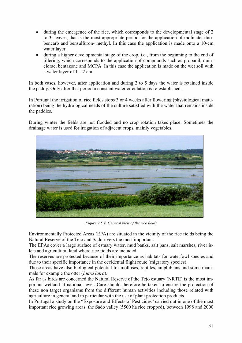
Figure 2.5.4. General view of the rice fields Environmentally Protected Areas (EPA) are situated in the vicinity of the rice fields being the Natural Reserve of the Tejo and Sado rivers the most important. The EPAs cover a large surface of estuary water, mud banks, salt pans, salt marshes, river is-lets and agricultural land where rice fields are included. The reserves are protected because of their importance as habitats for waterfowl species and due to their specific importance in the occidental flight route (migratory species). Those areas have also biological potential for molluscs, reptiles, amphibians and some mam-mals for example the otter (Lutra lutra). As far as birds are concerned the Natural Reserve of the Tejo estuary (NRTE) is the most im-portant wetland at national level. Care should therefore be taken to ensure the protection of these non target organisms from the different human activities including those related with agriculture in general and in particular with the use of plant protection products. In Portugal a study on the “Exposure and Effects of Pesticides” carried out in one of the most important rice growing areas, the Sado valley (5500 ha rice cropped), between 1998 and 2000

32

indicate that residues of molinate and chlorfenvinphos were among the pesticides most fre-quently found in rice paddies and also in drainage canals and Sado River. Although acute toxic effects were observed with invertebrates (Daphnia-magna) in the rice paddies – target area – mainly due to the application of chlorfenvinphos. No significant acute effects were ob-served with other compounds on invertebrates, algae (R. subcapitata) and bacteria (V. fis-cheri) in the drainage canals and in the river Sado (Pereira et al., 2000). In Table 2.5.1 an overview of rice cropping in Portugal is presented. Table 2.5.1: Overview of rice cropping strategies in Portugal.

Characteristic Portugal Soils: * texture Sandy Clay/ Clay loam/ Clay * % o.m. 2 – 3 * pH 5 – 7 * % clay 30 – 40 Drainage system Yes, 2 systems Water level 2 – 10 cm Water velocity: * drainage (outflow field) 2 – 2.5 l/s/ha * field (inflow field) 2 – 4 l/s/ha Flooding conditions April – Sept Time of closure of field 2 – 5 days Depth of drainage channels 1 – 2 m Crop rotation No Infiltration (leakage) rate 1 – 10 mm/d Usage of outflow water Occasionally for irrigation Aeroplane application Yes Irrigation system Yes Temperature (ºC) > 16 – 22 Aerobic/anaerobic conditions at interface Aerobic

33

2.6 Spain The main rice areas in Spain are shown in the following Figure 2.6.1.

Figure 2.6.1. Rice cropping areas in Spain. The cultivated surface depends mainly on the water availability in some areas, but the relative importance of the total average appears in the next Figure 2.6.2. The sizes of the different rice growing areas in Spain are indicated in Table 2.6.1. Table 2.6.1. Areas and sizes of Spanish rice cropping Area Size Sevilla marshes ≅30000 ha Extremadura area ≅20000 ha Tarragona DENP. ≅25000 ha Valencia ANP. ≅18000 ha Aragon (Huesca/Zaragoza) ≅5000 ha Navarra ≅2000 ha Murcia (Calasparra) ≅500 ha

There are two types of very different rice scenarios in Spain. The first ones are those that be-long to, or are near a Natural Park or Wild Life Reserve area, like Delta of Ebro Natural Park (DENP), Albufera Natural Park (ANP) and Sevilla Marshes (near Doñana Park). Secondly, those ones that are irrigated thanks to big channels from rivers or dams like the Extremadura, Aragon or Navarra areas. In this last situation, the procedure of irrigation is closer to the ce-real crops where leaching is very significant. In the others an impervious soil layer reduces

S

S

S

YY

Y

Y

#S#S

%U

%U

#S#S

#S

#S

Y

Oviedo

Madrid

Toledo

Merida

Murcia

Logrono

Sevilla

VitoriaPamplona

Zaragoza

Valencia

Santander

BarcelonaValladolid

Palma De Mallorca

Santiago De Compostela

SEVILLA MARSHES

EXTREMADURA AREA

MURCIA (CALASPARRA)

VALENCIA ANP

TARRAGONA DNP

ARAGON (HUESCA/ZARAGOZA)

Portugal

France

NAVARRA

Guad

iana R

Guadalquivir R

Jucar R

Ebro R

Segura R

2. RICE CROPPING IN EUROPE2.5. SPAIN

N

100 0 100 kilometers

37° 37°

39° 39°

41° 41°

43° 43°

9°

9°

7°

7°

5°

5°

3°

3°

1°

1°

1°

1°

3°

3°

34

leaching and then degradation must be considered the main way of dissipation. Both scenarios are called Flooded Paddies or Drained Paddies.

Figure 2.6.2. Relative importance of rice growing areas in Spain.

Figure 2.6.3. During the wintertime many of the rice fields are with water, as is normal

in a Mediterranean humid zone.

VALENCIA ANP

MAIN RICE AREAS IN SPAIN

MURCIA(Calasparra)

NAVARRA

ARAGON (Huesca/Zaragoza SEVILLA

MARSHES

TARRAGONA DENPEXTREMADURA AREA

35

Many of the rice soils are heavy, saline and hydromorfic. A complex net of irrigation and drainage channels is situated in all of these field areas.

Figure 2.6.4. One of the more important works in the Flooded Paddy

rice fields is done with special rotovator machines. The soil preparation starts, in wintertime, with a first deep ploughing, in February or March, then followed by harrowing, and levelling. Level of soil by laser, is a key factor for good irri-gation and also to control weeds. Sowing is done during the first days of May, spreading the seeds on the water. Some oxygenation of the rice plant is produced during one or two short dry periods in the sea-son. During this second period herbicides are applied. Chilo suppressalis is the main pest that sometimes is treated by aeroplane with fenitrothion or sexual confusion. Pyricularia oryzae is the principal disease, but some varieties and years do not need any treatment. The main weeds of two of the principal rice scenarios ANP and DENP are shown in the next Tables 2.6.2 and 2.6.3.

36

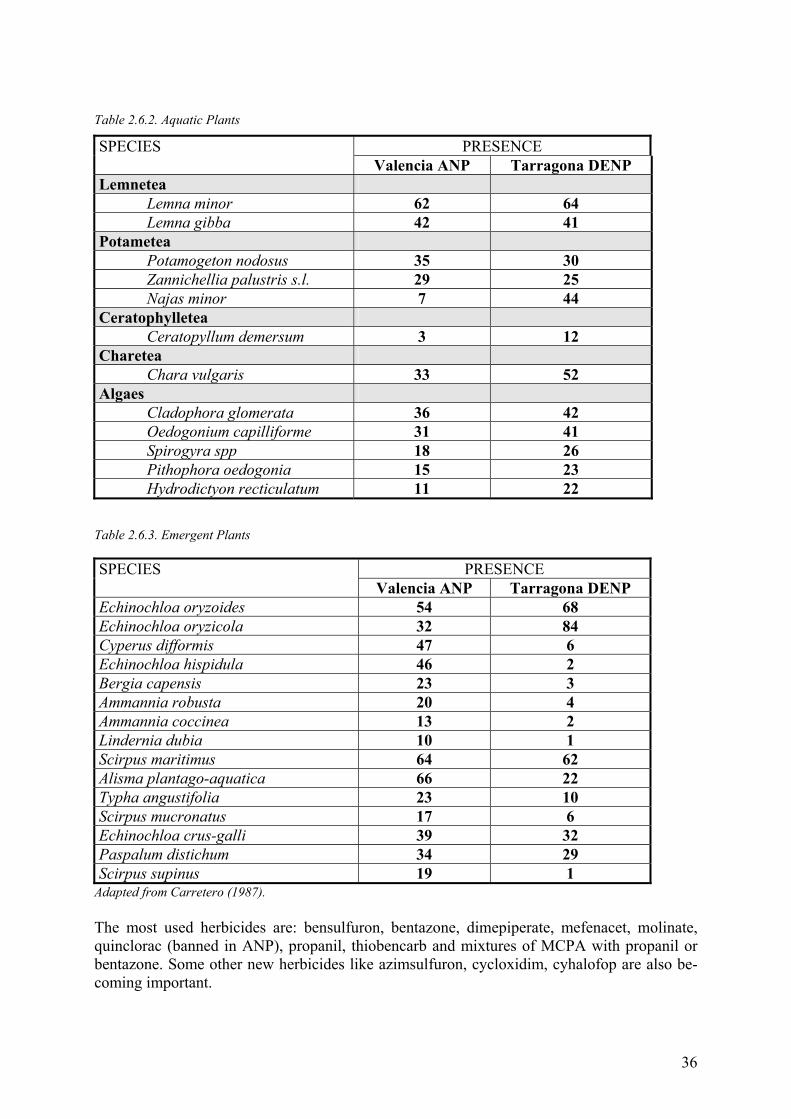
Table 2.6.2. Aquatic Plants

PRESENCE SPECIES Valencia ANP Tarragona DENP

Lemnetea Lemna minor 62 64 Lemna gibba 42 41 Potametea Potamogeton nodosus 35 30 Zannichellia palustris s.l. 29 25 Najas minor 7 44 Ceratophylletea Ceratopyllum demersum 3 12 Charetea Chara vulgaris 33 52 Algaes Cladophora glomerata 36 42 Oedogonium capilliforme 31 41 Spirogyra spp 18 26 Pithophora oedogonia 15 23 Hydrodictyon recticulatum 11 22

Table 2.6.3. Emergent Plants

PRESENCE SPECIES Valencia ANP Tarragona DENP

Echinochloa oryzoides 54 68 Echinochloa oryzicola 32 84 Cyperus difformis 47 6 Echinochloa hispidula 46 2 Bergia capensis 23 3 Ammannia robusta 20 4 Ammannia coccinea 13 2 Lindernia dubia 10 1 Scirpus maritimus 64 62 Alisma plantago-aquatica 66 22 Typha angustifolia 23 10 Scirpus mucronatus 17 6 Echinochloa crus-galli 39 32 Paspalum distichum 34 29 Scirpus supinus 19 1

Adapted from Carretero (1987). The most used herbicides are: bensulfuron, bentazone, dimepiperate, mefenacet, molinate, quinclorac (banned in ANP), propanil, thiobencarb and mixtures of MCPA with propanil or bentazone. Some other new herbicides like azimsulfuron, cycloxidim, cyhalofop are also be-coming important.

37

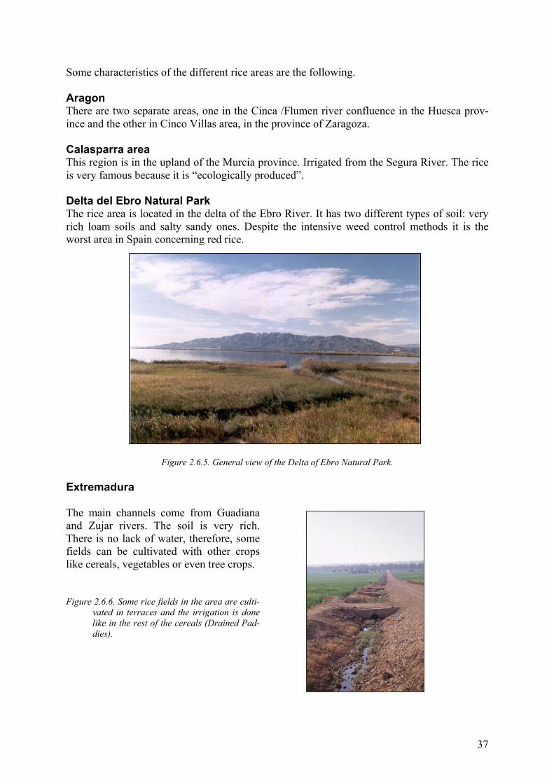
Some characteristics of the different rice areas are the following. Aragon There are two separate areas, one in the Cinca /Flumen river confluence in the Huesca prov-ince and the other in Cinco Villas area, in the province of Zaragoza. Calasparra area This region is in the upland of the Murcia province. Irrigated from the Segura River. The rice is very famous because it is “ecologically produced”. Delta del Ebro Natural Park The rice area is located in the delta of the Ebro River. It has two different types of soil: very rich loam soils and salty sandy ones. Despite the intensive weed control methods it is the worst area in Spain concerning red rice.

Figure 2.6.5. General view of the Delta of Ebro Natural Park.

Extremadura The main channels come from Guadiana and Zujar rivers. The soil is very rich. There is no lack of water, therefore, some fields can be cultivated with other crops like cereals, vegetables or even tree crops. Figure 2.6.6. Some rice fields in the area are culti-

vated in terraces and the irrigation is done like in the rest of the cereals (Drained Pad-dies).

38

Navarra The main area is located in Arguedas. Another less important area is located in Rada. Water for flood irrigation comes from channels of the Ebro River. Sevilla marshes In normal rainy years, rice is the only crop in the area. The actual rice surface is around 30000 ha. Irrigation is through channels taking water from Guadalquivir River that belongs to very im-portant growers associations. The characteristics of the soil are: heavy, clay or clay loam, pH 7 – 8.5, high calcium carbon-ate, organic matter 2 – 2.5%. Average size of the plots is 6 – 10 ha.

Figure 2.6.7. The size of the Sevilla marshes rice fields is larger

then in the rest of the scenarios in Spain. The main weeds are shown in the following Table 2.6.4. Table 2.6.4. Main weeds in rice crops. Weed type SPECIES

Cynodon dactylon Echinochloa crus galli Phragmites communis Paspalum distichum Scirpus maritimus

Narrow leafed weeds

Scirpus mucronatus Alisma plantago

Typha sp. Broad leafed weeds

Lemna minor Adapted from Borrero A. (1997). Albufera Natural Park The Albufera Natural Park of Valencia (ANP) is located in the South of Valencia city, be-tween the Turia and Jucar rivers. The total surface of the ANP is around 21120 ha. The lake has 2840 ha, but rice fields are around 18000 ha. There are two different sections, the rice fields affected by the level of the water in the lake ("tancats"), that are those fields close to the

39

lake, in which flooding depends of the level of the water in the lake, and other fields sur-rounding the first ones, that are directly irrigated from the Turia or Jucar river or pumping wa-ter from the lake. There is a complete net of irrigation channels and areas of 20 to 50 ha, named "tancats” that are surrounded by furrows allowing irrigation and drainage in common. Fauna of the ANP has many important species. For example two fishes, Lebias ibera and Va-lencia hispanica, are very sensible to water contamination. Avian population is also very im-portant because the ANP, like DENP, or SM/Doñana Park are humid key areas for migratory population. Weed control is done with the following chemicals and is shown in Table 2.6.5. Table 2.6.5. Weed control, treatment and chemicals used.

Weed Treatment Chemical a) Pre-flooding, spreading or spraying with molinate and immediately incor-porated

Molinate

b) Post emergence, 3 – 4 leaves, 2 – 3 weeks after flooding. After the treat-ment, 15 cm of level of water must be maintained for 2 – 3 days

Molinate thiobencarb dimepiperate mefenacet + molinate

c) Post emergence, 4 – 5 leaves, 6 – 7 weeks after sowing, during 2º drying

Propanil (2 treat-ments)

Echinochloa spp.

d) 1 – 3 leaves; almost without water in the field, but with water 24 h after treatment

Cyhalofop

Post emergence, 3 – 4 weeks after sow-ing, closing the inlet and outlet of the water for 3 – 5 days

Azimsulfuron, bensulfuron

Alisma spp, cy-peraceae, and dicot.

Post emergence, 7 – 8 weeks after sow-ing, at 2 days before drying

Bentazone bentazone + MCPA propanil + MCPA

Potamogeton nudosus

During the middle of the drying Bensulfuron, endhotal

Hetherantera spp

Is still not important Oxadiazon, pretilachlor

In the boundary of the fields Glyphosate, glufosi-nate, sulfosate

Paspalum disti-chum

In the rice field, after harvesting Glyphosate or sul-fosate

Adapted from Batalla J.A. (1994). The overview of rice cropping in Spain is given in Table 2.6.6

40

Table 2.6.6: Overview of rice cropping strategies in Spain.

Characteristic Spain Soils: * texture Clay/Loam/

Sandy loam * % o.m. 0.5 – 3 * pH 5.5 – 8.5 * % clay 10 – 40 Drainage system Yes Water level < 20 cm,

average 10 cm Water velocity: * drainage (outflow field) 0.15 l/s/ha * field (inflow field) 0.5 – 1.5 l/s/ha Flooding conditions April – Aug Time of closure of field 2 – 5 days Depth of drainage channels 2 m Crop rotation In some areas Infiltration (leakage) rate 1 – 10 mm/d Usage of outflow water No Aeroplane application Generally no Irrigation system Yes, flooding Temperature (ºC) > 14 – 20 Aerobic/anaerobic conditions at interface Aerobic

41

Figure 2.6.8. Valencia Albufera National Park

JÚCAR RIVER

TURIARIVER

MEDIT

ERRANEAN

SEA

VALENCIACITYVALENCIACITY

ALBUFERALAKEALBUFERALAKE

720000 725000 730000

730000

735000

735000

740000

740000

4335000

4340000 4340000

4345000 4345000

4350000 4350000

4355000 4355000

4360000 4360000

4365000 4365000

4370000 4370000

VALENCIA ALBUFERA NATURAL PARK

Source: COPUT. Generalitat Valenciana.

N

1 0 1 2 3 4kilometers

Rice fieldUrban area

42

2.7 Overview Based on the information in the preceding paragraphs the following overview Table 2.7.1 gives information concerning the rice cropping strategies in the South European countries. The main characteristics of the cropping are indicated to illustrate the similarities and differ-ences in these countries. Table 2.7.1. Overview of rice cropping strategies.

Characteristic France Greece Italy Portugal Spain Soils: * texture Silt loam/

Silty clay loam

Silty loam Clay/Sandy Sandy Clay/ Clay loam/

Clay

Clay/Loam/ Sandy loam

* % o.m. 1 – 4 1.8 – 2.0 0.8 – 10 2 – 3 0.5 – 3 * pH 8.0 7.4 – 8.0 4 – 8 5 – 7 5.5 – 8.5 * % clay 10 – 40 20 Sandy: 2 – 6

Clay: 20 – 30 30 – 40 10 – 40

Drainage system Yes Yes (75%) Yes Yes, 2 sys-tems

Yes

Water level Max. 20 cm, average 10

cm

2 – 10 cm 10 cm 2 – 10 cm < 20 cm, average 10

cm Water velocity: * drainage (outflow

field)

0.4 l/s/ha 0.5 l/s/ha 0.15 l/s/ha 2 – 2.5 l/s/ha 0.15 l/s/ha

* field (inflow

field)

2 – 3 l/s/ha 4 l/s/ha 1.01 l/s/ha 2 – 4 l/s/ha 0.5 – 1.5 l/s/ha

Flooding condi-tions

May – Aug May – Sept May – Sept April – Sept April – Aug

Time of closure of field

7 days 2 – 5 days 5 days 2 – 5 days 2 – 5 days

Depth of drainage channels

1.5 – 2.5 m 1.5 – 2.0 m 1 – 2 m 1 – 2 m 2 m

Crop rotation Yes Yes (80%) No No In some ar-eas

Infiltration (leak-age) rate

Max < 8 mm/d, Mean

4 mm/d

5 – 10 mm/d 6 – 11 mm/d 1 – 10 mm/d 1 – 10 mm/d

Usage of outflow water

No No No Occasionally for irrigation

No

Aerial application Yes No No Yes Generally no Irrigation system No Yes (75%) Yes, 3 sys-

tems Yes Yes, flooding

Temperature (ºC) > 14 > 12 > 14 > 16 – 22 > 14 – 20 Aerobic/anaerobic

conditions at soil/water inter-face

Aerobic Aerobic Aerobic Aerobic Aerobic

43

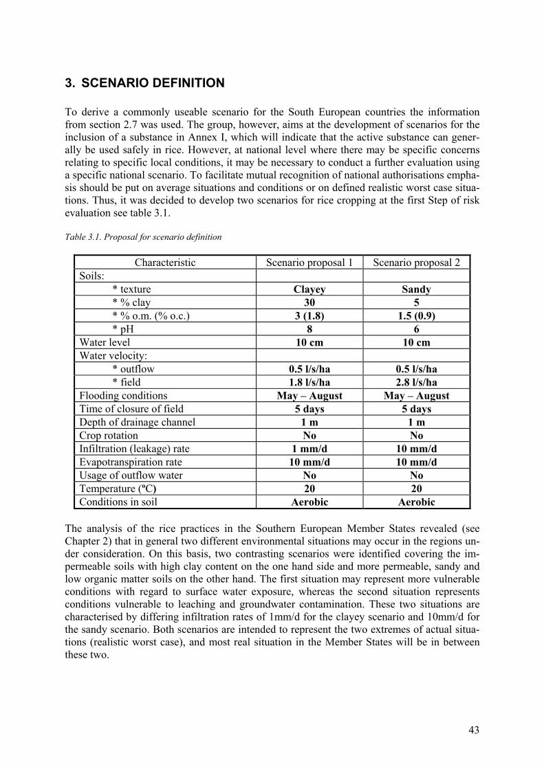
3. SCENARIO DEFINITION To derive a commonly useable scenario for the South European countries the information from section 2.7 was used. The group, however, aims at the development of scenarios for the inclusion of a substance in Annex I, which will indicate that the active substance can gener-ally be used safely in rice. However, at national level where there may be specific concerns relating to specific local conditions, it may be necessary to conduct a further evaluation using a specific national scenario. To facilitate mutual recognition of national authorisations empha-sis should be put on average situations and conditions or on defined realistic worst case situa-tions. Thus, it was decided to develop two scenarios for rice cropping at the first Step of risk evaluation see table 3.1. Table 3.1. Proposal for scenario definition

Characteristic Scenario proposal 1 Scenario proposal 2 Soils: * texture Clayey Sandy * % clay 30 5 * % o.m. (% o.c.) 3 (1.8) 1.5 (0.9) * pH 8 6 Water level 10 cm 10 cm Water velocity: * outflow 0.5 l/s/ha 0.5 l/s/ha * field 1.8 l/s/ha 2.8 l/s/ha Flooding conditions May – August May – August Time of closure of field 5 days 5 days Depth of drainage channel 1 m 1 m Crop rotation No No Infiltration (leakage) rate 1 mm/d 10 mm/d Evapotranspiration rate 10 mm/d 10 mm/d Usage of outflow water No No Temperature (ºC) 20 20 Conditions in soil Aerobic Aerobic

The analysis of the rice practices in the Southern European Member States revealed (see Chapter 2) that in general two different environmental situations may occur in the regions un-der consideration. On this basis, two contrasting scenarios were identified covering the im-permeable soils with high clay content on the one hand side and more permeable, sandy and low organic matter soils on the other hand. The first situation may represent more vulnerable conditions with regard to surface water exposure, whereas the second situation represents conditions vulnerable to leaching and groundwater contamination. These two situations are characterised by differing infiltration rates of 1mm/d for the clayey scenario and 10mm/d for the sandy scenario. Both scenarios are intended to represent the two extremes of actual situa-tions (realistic worst case), and most real situation in the Member States will be in between these two.

44

4. DATA REQUIREMENTS 4.1 Fate and Behaviour

4.1.1 Introduction The data requirements concerning environmental fate and behaviour are described in Com-mission Directive 95/36/EC, which defines the circumstances in which each study is required and also recommends the appropriate test guidelines. It is recognised that some of the guid-ance given in this Directive is not appropriate for plant protection products used in rice. Where possible, the guidance given in 95/36/EC has been retained but, where the study design is not relevant for rice paddies, amendments to the guidelines are recommended. More appro-priate study types as suggested in the following section should then replace the current re-quirements of Directive 95/36/EC. A scheme outlining the criteria for deciding which studies are required is shown in Figure 4.1.1.1. Note that this guidance applies only to plant protection products that are applied to flooded fields or to fields that are drained and re-flooded within a short period (7 days). For applica-tion under non-flooded conditions or to fields that are drained but not re-flooded within 7 days, current guidance (as described in 95/36/EC) should be followed.

4.1.2 Fate and Behaviour Studies – Annex II of Directive 91/414/EEC The following guidance is proposed for each 91/414/EEC Annex II point:

7.1 FATE AND BEHAVIOUR IN SOIL 7.1.1 Route and rate of degradation 7.1.1.1 Route of degradation 7.1.1.1.1 Aerobic degradation in soil

Conduct flooded aerobic soil degradation study based on SETAC guideline 1.1 and as described for rice paddy soils in OECD Test Guideline 307 for aerobic and anaerobic transformation in soil. One typical representative rice soil (e.g. clay or clay loam) should be used. Soils should be flooded with 5 – 10 cm depth of water with a soil : water ratio of 1:1. Soil should be flooded 7 days prior to application of active substance.

7.1.1.1.2 Supplementary studies Anaerobic degradation in soil

Current guidance acceptable.

Photolysis in soil Current guidance acceptable.

45

7.1.1.2 Rate of degradation 7.1.1.2.1 Laboratory studies on rate of degradation in soil

Aerobic degradation Conduct flooded aerobic soil degradation study as described in 7.1.1.1.1 using one additional soil (e.g. a sandy soil). Separate DT50 values should be determined for the water and soil compartments.

Anaerobic degradation Current guidance acceptable. Data will be obtained from study described in 7.1.1.1.2.

7.1.1.2.2 Field studies on rate of degradation in soil Soil (paddy) dissipation

Required if

(i) the DT50lab in the whole soil/water system of the flooded aerobic soil degrada-tion study is greater than 60 days

or

(ii) the DT50lab in the whole soil/water system of the flooded aerobic soil degrada-tion study is lower than 60 days and there is an unacceptable risk to aquatic organisms in the non-target area.

Small-scale outdoor flooded soil studies and/or full-scale field dissipation studies should be carried out. Study design for the full-scale field study should be based broadly on SETAC guideline 3.1 but should use rice paddies at two locations. Normal agricultural practices should be followed as closely as possible. Soil from the paddy field and water from the field and from the outflow should be sampled and analysed. Separate DT50field and DT90field values should be calculated for soil and water if possible.

In cases where photolysis could be an important route of degradation, a small-scale outdoor flooded soil study may be conducted using radiolabelled material. If the DT50 from this study still exceeds the trigger values above, then full scale field dissipation studies should be carried out.

Soil residue Not required for rice products since it is not common practice to plant rotational crops in the same year.

Soil accumulation Required if DT90field in the soil from the soil dissipation study is greater than one year. Study design should be agreed with the relevant regulatory authority. The general approach and testing strategies should be in-line with the Guidance Document on Persistence (Commission Document 9188/VI/97 current Revision 8).

7.1.2 Adsorption and desorption Current guidance acceptable.

46

7.1.3 Mobility in the soil 7.1.3.1 Column leaching studies

Current guidance is considered acceptable.

7.1.3.2 Aged residue column leaching studies Current guidance is considered acceptable.

7.1.3.3 Lysimeter studies or field leaching studies Expert judgement required to decide if required. Study design should be agreed with the relevant regulatory authority.

7.2 FATE AND BEHAVIOUR IN WATER AND AIR 7.2.1 Rate and route of degradation in aquatic systems 7.2.1.1 Hydrolytic degradation

Current guidance is considered acceptable.

7.2.1.2 Photochemical degradation 7.2.1.3.1 Ready biodegradability

Current guidance is considered acceptable.

7.2.1.3.2 Water/sediment study Current guidance is considered acceptable.

7.2.1.4 Degradation in the saturated zone Expert judgement required to decide if required. Study design should be agreed with the relevant regulatory authority.

7.2.2 Rate and route of degradation in air No specific guideline required for rice use. Current guidance is considered acceptable.

7.3 DEFINITION OF THE RESIDUE Current guidance is considered acceptable.

7.4 MONITORING DATA Current guidance is considered acceptable.

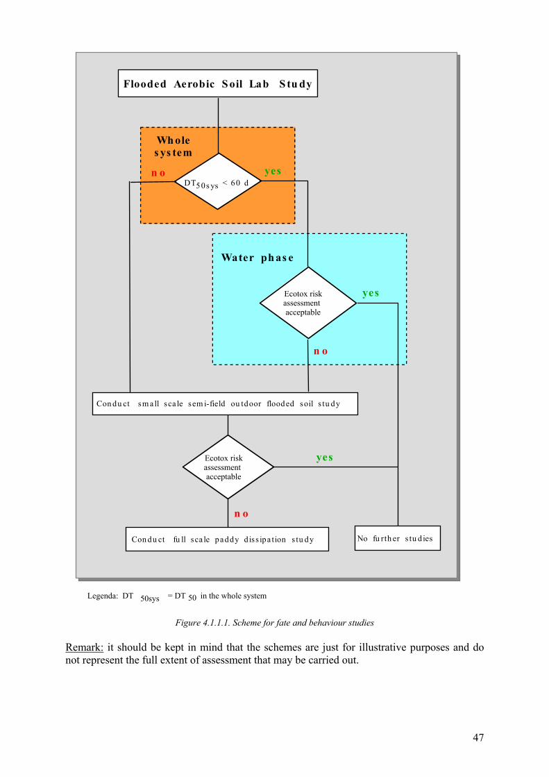
47

Figure 4.1.1.1. Scheme for fate and behaviour studies

Remark: it should be kept in mind that the schemes are just for illustrative purposes and do not represent the full extent of assessment that may be carried out.

Legenda: DT 50sys = DT 50 in the whole system

n o

Flooded Aerobic S oil Lab S tu dy

yes

yesEcotox riskassessmentacceptable

Con du ct fu ll sca le paddy d iss ipa tion s tu dy

Con du ct sm all sca le sem i-field ou tdoor flooded soil s tu dy

Wh oles ys tem

DT50s ys < 60 d

Water ph as e

No fu rth er s tu d ies

n o

Ecotox riskassessmentacceptable

n o yes

yes

48

4.2 Ecotoxicology

4.2.1 Introduction The ecotoxicological data requirements are described in the Commission Directive 96/12/EC which defines the circumstances in which each study is required and also recommends the appropriate test guidelines if available. Nevertheless, it is recognised that some clarifications were needed for active substances to be used in rice culture. If considered acceptable the guidance given in 96/12/EC Directive has been retained but in a few cases some amendments to the guidelines seem to be justified and they are now recom-mended below. The Guidance Documents on Ecotoxicology that were recently made avail-able need also to be taken into consideration, in particular the Guidance Document on Aquatic Ecotoxicology (SANCO, 2000, 2001 and 2002) and the recommendations of ESCORT 2 (ESCORT, 2001).

4.2.2 Ecotoxicological Studies – Annex II of Directive 91/414/EEC The following ecotoxicological data requirements are proposed to take into consideration for inclusion of an active substance in Annex I of the Directive 91/414/EEC.

8.1 EFFECTS ON BIRDS 8.1.1 Acute oral toxicity

Current guidance is considered acceptable. (SANCO, 2000)

8.1.2 Short term dietary toxicity Current guidance is considered acceptable. (SANCO, 2000)

8.1.3 Subchronic toxicity and reproduction Current guidance is considered acceptable. (SANCO, 2000)

8.2 EFFECTS ON AQUATIC ORGANISMS 8.2.1 Acute toxicity to fish

Current guidance is considered acceptable. (SANCO, 2001)

8.2.2 Chronic toxicity to fish Current guidance is considered acceptable. (SANCO, 2001). Chapters 4 and 5 of Guidance Document 3268/2001, rev.4, final on Aquatic Ecotoxicology should be followed. (SANCO, 2001)

8.2.3 Bioconcentration to fish Current guidance is considered acceptable. Section 5.7 of Guidance Document 3268/2001, rev.4, final on Aquatic Ecotoxicology should be followed.

8.2.4 Acute toxicity to aquatic invertebrates Current guidance is considered acceptable. (SANCO, 2001)

8.2.5 Chronic toxicity to aquatic invertebrates Current guidance is considered acceptable. (SANCO, 2001)

49

8.2.6 Effects on algae growth Current guidance is considered acceptable. (SANCO, 2001)

8.2.7 Effects on sediment dwelling organisms Current guidance is considered acceptable. (SANCO, 2001)

8.2.8 Aquatic plants Current guidance is considered acceptable. (SANCO, 2001)

8.3 EFFECTS ON ARTHROPODS 8.3.1 Bees 8.3.1.1 Acute toxicity

Current guidance is considered acceptable. The likelihood of exposure of bees should be justified. (ESCORT 2, 2001)

8.3.1.2 Bee brood feeding test Current guidance is considered acceptable. The likelihood of exposure of bees should be justified. (ESCORT 2, 2001)

8.3.2 Other arthropods Current guidance acceptable. (ESCORT 2, 2001)

8.4 EFFECTS ON EARTHWORMS 8.4.1 Acute toxicity

Current guidance is considered acceptable. (SANCO, 2002)

8.4.2 Sublethal effects Current guidance is considered acceptable. (SANCO, 2002)

8.5 EFFECTS ON SOIL NON-TARGET MICRO-ORGANISMS For the moment the current guidance is considered acceptable. The use of one typical rice soil to perform the tests and the need for a study under flooded condi-tions are still considered open points. When more precise guidance on these items becomes available this should be taken into consideration.

8.6 EFFECTS ON OTHER NON-TARGET ORGANISMS (FLORA AND FAUNA) BELIEVED TO BE AT RISK

Current guidance is considered acceptable. (SANCO, 2002)

8.7 EFFECTS ON BIOLOGICAL METHODS FOR SEWAGE TREAT-MENT

Current guidance is considered acceptable. (SANCO, 2001)

50

4.2.3 Ecotoxicological Studies – Annex III of Directive 91/414/EEC

10.1 EFFECTS ON BIRDS Current guidance is considered acceptable. (SANCO, 2000)

10.2 EFFECTS ON AQUATIC ORGANISMS Current guidance is considered acceptable. (SANCO, 2001)

10.3 EFFECTS ON TERRESTRIAL VERTEBRATES OTHER THAN BIRDS

Current guidance is considered acceptable. (SANCO, 2002)

10.4 EFFECTS ON BEES Current guidance is considered acceptable. See comment under point 8.3.1. (ES-CORT 2, 2001)

10.5 EFFECTS ON ARTHROPODS OTHER THAN BEES Current guidance is considered acceptable. (ESCORT 2, 2001)

10.6 EFFECTS ON EARTHWORMS AND OTHER SOIL NON-TARGET MACRO-ORGANISMS BELIEVED TO BE AT RISK

Current guidance is considered acceptable. (SANCO, 2002)

10.7 EFFECTS ON SOIL NON-TARGET MICRO-ORGANISMS Current guidance is considered acceptable. See comment under point 8.5. (SANCO, 2002)

10.8 AVAILABLE DATA FROM BIOLOGICAL PRIMARY SCREENING IN SUMMARY FORM

Current guidance is considered acceptable.

4.2.4 Risk Assessment The methods proposed for calculation of PECs as required by the Directive 91/414/EEC are described in Chapter 5 for surface water, sediment, groundwater and soil. These PEC values are used for the risk assessment in the relevant compartments. For Annex I listing, the current guidance provided in the Uniform Principles on risk assess-ment for non-target species is applied. No additional ecotoxicological testing is proposed for rice in comparison with the normal procedure for other cultures and there is no reason to change the current trigger values for TERs (Toxicity Exposure Ratios) or HQs (Hazard Quo-tients) for non-target terrestrial organisms. Potential effects to these species need to be con-sidered, as they are under 91/414 for other agricultural scenarios. If a TER or HQ trigger is not met in the initial assessment then higher tier assessments will be required as described in the existing Guidance Documents on Terrestrial Ecotoxicology (SANCO/10329/2002, REV.2, 17 October 2002), ESCORT 2 (M.P. Candolfi, K.L. Barrett, P.J. Campbell et.al. 2000) and for Birds and Wild Mammals (SANCO/4145/2000, 25 September 2002).

51

For aquatic organisms, the current trigger values for TERs as prescribed under 91/414 should be applied for the “off-field” environment. Where a TER trigger is not met in the ini-tial assessment, a higher tier assessment will be required as described in the existing Guidance Document on Aquatic Ecotoxicology (SANCO/3268/2001, REV.4, 17 October 2002) or in the recommendations of the HARAP (Campbell & al 1999) and CLASSIC (Giddings & al 2002) workshops. A similar risk assessment for aquatic organisms in the rice field itself is generally not appropriate because applying the same protection goals to the “in-field” target area as are applied to the “off-field” non-target area is inappropriate for a rice paddy, which falls dry after a certain time period. In a flooded rice field some effect on non-target aquatic plant and invertebrate species will be inevitable as a result of herbicide and insecticide use when both the target and the non-target species are physiologically related. Member States should perform specific “in-field” aquatic risk assessments after Annex I inclusion to take into consideration specific local conditions, agricultural practices and particular aspects of environmental protection (e.g. in cases where paddies are located close to protected areas or irrigation water is feeding into protected water bodies).

52

5. PEC CALCULATIONS 5.1 Definitions This section describes the various procedures used for calculating the predicted environmental concentration of an active substance in the different environmental compartments (soil, sur-face water, sediment and groundwater). It is important to note that, in this guidance document, the term “surface water“ refers to water in non-target areas (e.g. drainage canals) whereas the term ″paddy water“ is used for water in the cropped field. Similarly, the term ″sediment“ re-fers to sediment associated with surface water in non-target areas and the term ″soil“ is used only for the cropped field. For the purposes of the initial PEC calculations, ″groundwater“ is defined as water in the saturated zone 1m below the soil surface. In general, the different environmental fate studies proposed under the data requirements should provide sufficient information regarding the degradation of a product in different envi-ronmental matrices. The corresponding DT50 values derived from these studies can be used for the PEC calculations. Generally, the fate and behaviour of a compound should be assessed under consideration of all available data from different studies / study types. In the first step and if results from dif-ferent studies do not suggest otherwise, the use for PEC calculations is considered as follows:

paddy field (PECpw, PECsoil, PECpgw) → flooded aerobic soil degradation receiving canal (PECsw, PECsed) → aerobic aquatic water / sediment study.

It should be noted that assumptions used throughout the document as especially this section are in line with other guidance documents for risk assessments for PPPs. Some more specific assumptions for rice paddies are based on expert judgement with the inherent consequence that the values chosen or proposed are not covering all situations. If the specific situation re-quires a different value the deviation from the guidance should be explicitly mentioned in the evaluation and justified. In such cases automatically a higher tier risk assessment should be carried out. As this kind of default values have an arbitrary character further justification of the choice is not possible. Therefore, some assumptions have a pragmatic character for regula-tory assessment and risk management. However, where it is possible a further justification will be given. For the selection of data from the dossier of the active substance guidance is given in the re-port of the FOCUS Working Group on Surface Water Scenarios (FOCUS, 2002). The MED-Rice group fully supports the guidance given there. Especially, for the selection of biodegra-dation data, DT50-values, it should be kept in mind that in principle separate DT50-values are needed for the description of the degradation in the water phase and in the sediment phase. Often this will not be possible. In such a case the overall DT50 of the water/sediment system should be used for the water as well as for the sediment phase.

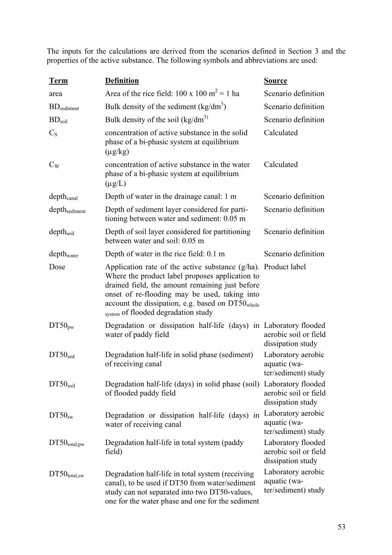
53

The inputs for the calculations are derived from the scenarios defined in Section 3 and the properties of the active substance. The following symbols and abbreviations are used: Term Definition Source

area Area of the rice field: 100 x 100 m2 = 1 ha Scenario definition

BDsediment Bulk density of the sediment (kg/dm3) Scenario definition

BDsoil Bulk density of the soil (kg/dm3) Scenario definition

CS concentration of active substance in the solid phase of a bi-phasic system at equilibrium (µg/kg)

Calculated

CW concentration of active substance in the water phase of a bi-phasic system at equilibrium (µg/L)

Calculated

depthcanal Depth of water in the drainage canal: 1 m Scenario definition

depthsediment Depth of sediment layer considered for parti-tioning between water and sediment: 0.05 m

Scenario definition

depthsoil Depth of soil layer considered for partitioning between water and soil: 0.05 m

Scenario definition

depthwater Depth of water in the rice field: 0.1 m Scenario definition

Dose Application rate of the active substance (g/ha). Where the product label proposes application to drained field, the amount remaining just before onset of re-flooding may be used, taking into account the dissipation, e.g. based on DT50whole

system of flooded degradation study

Product label

DT50pw Degradation or dissipation half-life (days) in water of paddy field

Laboratory flooded aerobic soil or field dissipation study

DT50sed Degradation half-life in solid phase (sediment) of receiving canal

Laboratory aerobic aquatic (wa-ter/sediment) study

DT50soil Degradation half-life (days) in solid phase (soil) of flooded paddy field

Laboratory flooded aerobic soil or field dissipation study

DT50sw Degradation or dissipation half-life (days) in water of receiving canal

Laboratory aerobic aquatic (wa-ter/sediment) study

DT50total,pw Degradation half-life in total system (paddy field)

Laboratory flooded aerobic soil or field dissipation study

DT50total,sw Degradation half-life in total system (receiving canal), to be used if DT50 from water/sediment study can not separated into two DT50-values, one for the water phase and one for the sediment

Laboratory aerobic aquatic (wa-ter/sediment) study

54

phase.

factdilution Dilution factor of paddy water reaching adjacent surface water: 10

Scenario definition

fdep Fraction of the dose deposited on the paddy wa-ter (i.e. 1 - fintercept)

Depending upon crop development / GAP

Fdissolved dissolved mass fraction Calculated

fdrift Fraction drift to adjacent surface water Drift tables

fintercept Fraction of the dose intercepted by the rice crop Depending upon crop development / GAP

Fsorbed sorbed mass fraction Calculated

KD Linear sorption coefficient (dm3/kg) Sorption study

KOC Sorption coefficient normalised to organic car-bon content (dm3/kg)

Sorption study

KOM Sorption coefficient normalised to organic mat-ter content (dm3/kg)

Sorption study

Leakage Infiltration rate (mm/day) Scenario definition

Mleak Total mass potentially available for leaching (Mleak,field + Mleak,flood) (g/ha)

Calculated

Mleak,field Mass potentially available for leaching during closure time tclose (g/ha)

Calculated

Mleak,flood Mass potentially available for leaching during flooding time tflood (g/ha)

Calculated

MS mass in sediment phase of the water/sediment system

Calculated

MT total mass in the water/sediment system Calculated

MW mass in water phase of the water/sediment sys-tem

Calculated

OC organic carbon content (%) Scenario definition

OM organic matter content (%) Scenario definition

Outflow rate Rate of water outflow from the paddy field (1/days)

Calculated

Outflow Amount of water leaving the paddy (L/s/ha) Scenario definition

PECpgw Predicted annual average concentrations in the saturated zone below the paddy (µg/L)

Calculated

PECpw Predicted concentration in paddy water (µg/L) Calculated

PECpw,end-close Concentration in paddy water at end of closure period tclose (µg/L)

Calculated

PECpw,end-flood Concentration in paddy water at end of flooding period tflood (µg/L)

Calculated

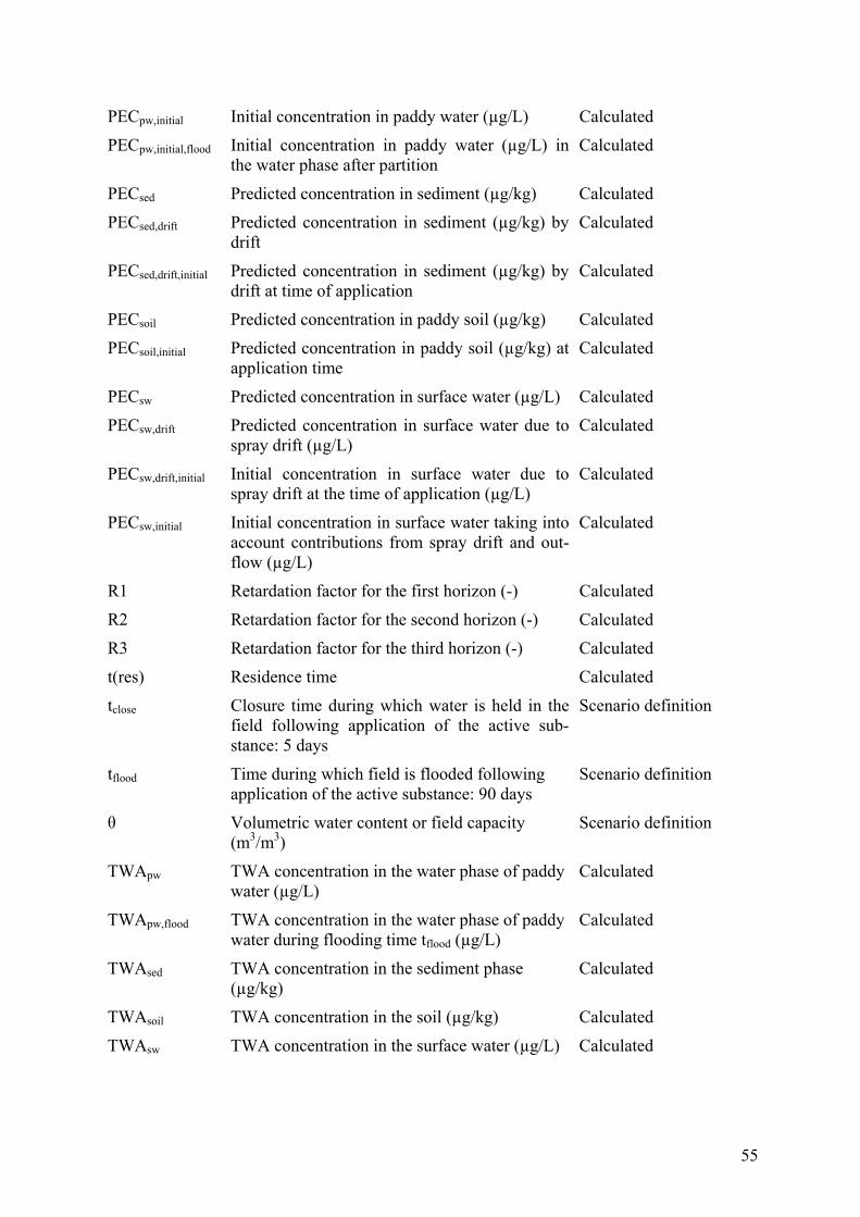
55

PECpw,initial Initial concentration in paddy water (µg/L) Calculated

PECpw,initial,flood Initial concentration in paddy water (µg/L) in the water phase after partition

Calculated

PECsed Predicted concentration in sediment (µg/kg) Calculated

PECsed,drift Predicted concentration in sediment (µg/kg) by drift

Calculated

PECsed,drift,initial Predicted concentration in sediment (µg/kg) by drift at time of application

Calculated

PECsoil Predicted concentration in paddy soil (µg/kg) Calculated

PECsoil,initial Predicted concentration in paddy soil (µg/kg) at application time

Calculated

PECsw Predicted concentration in surface water (µg/L) Calculated

PECsw,drift Predicted concentration in surface water due to spray drift (µg/L)

Calculated

PECsw,drift,initial Initial concentration in surface water due to spray drift at the time of application (µg/L)

Calculated

PECsw,initial Initial concentration in surface water taking into account contributions from spray drift and out-flow (µg/L)

Calculated

R1 Retardation factor for the first horizon (-) Calculated

R2 Retardation factor for the second horizon (-) Calculated

R3 Retardation factor for the third horizon (-) Calculated

t(res) Residence time Calculated

tclose Closure time during which water is held in the field following application of the active sub-stance: 5 days

Scenario definition

tflood Time during which field is flooded following application of the active substance: 90 days

Scenario definition

θ Volumetric water content or field capacity (m3/m3)

Scenario definition

TWApw TWA concentration in the water phase of paddy water (µg/L)

Calculated

TWApw,flood TWA concentration in the water phase of paddy water during flooding time tflood (µg/L)

Calculated

TWAsed TWA concentration in the sediment phase (µg/kg)

Calculated

TWAsoil TWA concentration in the soil (µg/kg) Calculated

TWAsw TWA concentration in the surface water (µg/L) Calculated

56

5.2 PEC in surface water, including Sediment

5.2.1 Introduction – Tiered Approach The calculation of predicted environmental concentrations (PECs) in the context of the regis-tration of plant protection products normally follows a step wise or tiered approach, starting with relatively simple “worst case” assumptions and models at the first step and progressing to more complex and more realistic models at later steps as appropriate. This approach has been followed and recommended by the FOCUS Working Groups on Leaching Models (Commission document 4952/VI/95), on Surface Water Modelling (Commission document 6476/VI/96) and on Soil Modelling (Commission document 7617/VI/96). A similar stepwise approach is being proposed for the exposure assessment in the case of plant protection products being used in rice cultures. In Figure 5.1.1.1. a schematic represen-tation of this approach is given. It was chosen to work with 3 steps in the exposure assessment process. The first step is based on simple assumptions regarding geometry and size of rice fields or adjacent surface water bodies as well as the distribution and dissipation of the product in the environment. Although these assumptions are relatively simple, they represent current ap-proaches for the surface water exposure assessment in other agricultural situations on a worst case basis. The first step is divided into three sub-steps, which distinguish between the exclusion or in-clusion of degradation and sorption and between different methods regarding the derivation of the respective degradation or dissipation rates from the experimental data. They are consid-ered to represent a stepwise refinement of the first exposure assessment Step. At higher Steps, modelling with more complex simulation models or site specific considera-tions are proposed. An overview of existing models, which could be used as a tool to estimate PECs in surface water, soil and sediment is given. The need to proceed further on the tiered approach will depend upon the results (safety) of the risk assessment for aquatic organisms. Therefore, the risk assessment should include the exposure assessment as proposed in this chapter in close relation with the hazard assessment as described in the guidance documents on Aquatic (SANCO, 2001) and Terrestrial (SANCO, 2002) Ecotoxicology and ESCORT 2 (ESCORT 2, 2001).

57

Figure 5.1.1.1. The Tiered Approach in Exposure Assessment of Plant Protection Products in Surface Waters.

Remark: it should be kept in mind that the schemes are just for illustrative purposes and do not represent the full extent of assessment that may be carried out.

yes

no

U sesafe ?

START

yes

no

U sesafe ?

yes

no

U sesafe ?

yes

no

U sesafe ?

Loading based on outflow anddrift, no degradation, no distribution

(sorption)

Loadings as in step 1a,degradation, no distribution

(sorption)

Loadings as in step 1a,degradation and distribution

(sorption)

Loadings as in step1,advanced modelling using

a simulation model

S TE P 1 a

S TE P 1 b

S TE P 1 c

S TE P 2

S T EP 3Realistic loadings, specific and

realistic description of site usingrealistic description

no furtherwork

58

5.2.2 Methods proposed – Step 1a, 1b and 1c The Step 1 PEC calculations for surface water and sediment are based on relatively simple assumptions regarding the paddy field environment. The conceptual scenario description is illustrated in Figure 5.1.2.1. Step 1a represents the simplest case, in that only initial concentrations are derived, and no fur-ther dissipation processes are considered. Step 1b and step 1c both consider additional dissipation processes such as degradation and/or sorption. Their appropriate use depends, however, on deriving the correct input parameters (e.g. DT50, KOC) from the respective experiments (e.g. flooded soil degradation study).

Figure 5.1.2.1. Conceptual scenario description for Step 1 Surface Water Calculations.

a) Step 1a, No degradation, no sorption The approach presented is according to the proposal of Azimonti et al. (1998). The following assumptions are proposed for the calculation of the PEC in paddy fields in the Step 1a estimation:

• Area of rice field: area = 1 ha = 104 m2 • Depth of water in field: depthwater = 0.1 m • Depth of receiving canals: depthcanal = 1 m • Dosage: Dose, according to the label (g/ha) • Fraction deposited on paddy water: fdep = 1 (conservative assumption)

Paddy soil – 5 cm depth considered for partitioning from water

Paddy water – 10 cm depth Surface water 100 cm depth

Sediment

5 cm depth considered for

partitioning

Outflow to surface water / canal

Spray drift at time of applica-tion

Application of the product to flooded paddy field

Paddy field size 100 x 100 m2

59

• Fraction drift to adjacent surface waters: fdrift = 0.0277 (example), this value should be adapted as the situation requires so according to FOCUS, 2001 or BBA, 2000).

• Fraction drift to adjacent surface waters: fdrift = 0.332 (example for aeroplane ap-plication), (FOCUS, 2001).

• Closure time as defined in Chapter 3 tclose = 5 days • Relevant processes: no degradation, no sorption at Step 1a • Mixing in surface water: complete mixing.

The value for drift is based on the most recent data issued in the FOCUS (2001 and the Guid-ance Document on Aquatic Ecotoxicology7. Using these assumptions, the predicted concentration in the paddy water (PECpw,initial), will be according to the following formula:

water

depinitialpw depth

DosefPEC

⋅⋅= 1.0, (1)

It should be noted that all water concentrations are expressed in µg/L. The parameter “fdep” may be interpreted as a contribution caused by interception by the crop, and is equal to 1 – fintercept (see Chapter 5.2.2). The initial concentration in the receiving canals due to spray drift at the time of application would be:

canaldriftinitialdriftsw depthfDosePEC /1.0,, ⋅⋅= (2) When the water from the field is discharged (drained) to the receiving canals, dilution is as-sumed to take place (factdilution = 10). The resulting total estimated concentration in the receiv-ing canals would be the sum of the contribution of drift and of discharge:

)1/()( ,,,, dilutioninitialpwdilutioninitialdriftswinitialsw factPECfactPECPEC ++⋅= (3)

b) Step 1b, Degradation no sorption According to common water and rice management practice, the water is allowed to stay some time within the paddy field before being discharged to the outflow canals. For many situa-tions, this closure time would be approximately 5 days. During that time, already dissipation of the substance may take place before the water from the field reaches the receiving canals, thus reducing the actual concentration in the paddy water. This process can be described using appropriate DT50 values from the relevant aerobic flooded soil degradation or field dissipation study. If it is not possible to obtain separate values for the DT50 in water and the DT50 in sediment from the water/sediment study of the dossier, the DT50total,sw from that study should be used for both DT50-values. When first order dissipation kinetics can describe the behaviour of the respective product ap-propriately, the time course of the concentration in the paddy water can be described by

7 http://europa.eu.int/comm/food/fs/ph_ps/pro/wrkdoc/index_en.htm

60

pwDTtinitialpwpw ePECtPEC 50/2ln

,)( ⋅−⋅= (4) Replacing t by the typical closure time tclose of the paddy field yields the actual paddy water concentration at onset of outflow:

pwDTtcloseinitialpwclosepw ePECtPEC 50/2ln

,)( ⋅−⋅= (5) At the same time, the fraction of the applied dose entering the canals by drift may have de-graded during the same period of time, resulting in:

swDTtcloseinitialdriftswclosedriftsw ePECtPEC 50/2ln

,,, )( ⋅−⋅= (6) The resulting concentration in the receiving canals due to drift and outflow at the time of field opening is then given by:

)1/())()(()( , dilutionclosepwdilutionclosedriftswclosesw facttPECfacttPECtPEC ++⋅= (7) Also in step 1b it is assumed that no sorption to the sediment takes place and therefore there is no exposure to the sediment. It should be noted, however, that at this step it may be justified to use the dissipation half-life rather then the pure degradation half-life. In that case, dissipa-tion from the water phase may well include processes of distribution, e.g. to sediment or soil.

c) Step 1c, Degradation and sorption In addition to step 1b, partitioning between water and sediment is taken into consideration. At this step it is essential that pure degradation half lives are used, in order not to double account for the dissipation from water due to partitioning to the soil or sediment. Sorption between water and sediment is assumed to be an instantaneous process determined by the sorption coefficient KD (dm3/kg). Therefore, the total amount of substance entering the water (MT) is distributed over the solid, e.g. soil or sediment phase (Msed and Csed) and liquid phase (Mw and Cw) according to the formulas, in which the first part refers to the amount (mass) and the second part to the concentration:

wDsswT CKCandMMM ⋅=+= (8) The sorption coefficient is calculated from the Koc or Kom according to:

100100OMK

KorOCK

K omD

ocD

⋅=

⋅= (8a)

The amount sorbed depends on the amount of water and soil or sediment. This may be de-scribed by the following equation in which Fdissolved is the mass fraction dissolved in the water phase and Fsorbed is the mass fraction sorbed to the solid phase:

dissolvedsorbedDentsewater

waterdissolved FFand

KBDdepthdepthdepth

F −=⋅⋅+

= 1dim

(9)

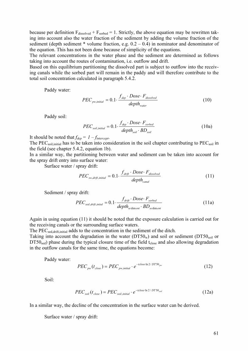
61

because per definition Fdissolved + Fsorbed = 1. Strictly, the above equation may be rewritten tak-ing into account also the water fraction of the sediment by adding the volume fraction of the sediment (depth sediment * volume fraction, e.g. 0.2 – 0.4) in nominator and denominator of the equation. This has not been done because of simplicity of the equations. The relevant concentrations in the water phase and the sediment are determined as follows taking into account the routes of contamination, i.e. outflow and drift. Based on this equilibrium partitioning the dissolved part is subject to outflow into the receiv-ing canals while the sorbed part will remain in the paddy and will therefore contribute to the total soil concentration calculated in paragraph 5.4.2.

Paddy water:

water

dissolveddepinitialpw depth

FDosefPEC

⋅⋅⋅= 1.0, (10)

Paddy soil:

soilsoil

sorbeddepinitialsoil BDdepth

FDosefPEC

⋅

⋅⋅⋅= 1.0, (10a)

It should be noted that fdep = 1 – fintercept. The PECsoil,initial has to be taken into consideration in the soil chapter contributing to PECsoil in the field (see chapter 5.4.2, equation 1b). In a similar way, the partitioning between water and sediment can be taken into account for the spray drift entry into surface water:

Surface water / spray drift:

canal

dissolveddriftinitialdriftsw depth

FDosefPEC

⋅⋅⋅= 1.0,, (11)

Sediment / spray drift:

entseentse

sorbeddriftinitaldriftsed BDdepth

FDosefPEC

dimdim,, 1.0

⋅

⋅⋅⋅= (11a)

Again in using equation (11) it should be noted that the exposure calculation is carried out for the receiving canals or the surrounding surface waters. The PECsed,drift,initial adds to the concentration in the sediment of the ditch. Taking into account the degradation in the water (DT50w) and soil or sediment (DT50soil or DT50sed) phase during the typical closure time of the field tclose and also allowing degradation in the outflow canals for the same time, the equations become:

Paddy water: pwDTtclose

initialpwclosepw ePECtPEC 50/2ln,)( ⋅−⋅= (12)

Soil:

soilDTtclose

initialsoilclosesoil ePECtPEC 50/2ln,)( ⋅−⋅= (12a)

In a similar way, the decline of the concentration in the surface water can be derived.

Surface water / spray drift:

62

swDTtcloseinitialdriftswclosedriftsw ePECtPEC 50/2ln

,,, )( ⋅−⋅= (13) Sediment / spray drift:

sedDTtcloseinitialdriftsedclosedriftsed ePECtPEC 50/2ln

,,, )( ⋅−⋅= (13a) Values for the respective DT50 in the water and soil or sediment phase should be taken from the appropriate degradation studies in flooded soil and sediment water systems. Finally, the resulting total concentration in the receiving surface water due to the contribution of outflow and drift are determined by summing both:

sedseddilution

sorbedwaterclosepwclosedriftsedclosesed

dilutionclosepwdilutionclosedriftswclosesw

BDdepthfactFdepthtPEC

tPECtPEC

and

facttPECfacttPECtPEC

⋅⋅⋅⋅

+=

++⋅=

)()()(

)1/())()(()(

,

,

(14)

It should be noted that, except for very rapidly degrading compounds, the original contribu-tion of spray drift at time = 0 to the receiving canals is considered to be negligible compared to the amount coming from the field after time = tclose. A sediment depth of 5 cm has been chosen because such a depth would realistically be the smallest depth that could be sampled from a field study for possible validation purposes. A smaller sediment depth would be diffi-cult to sample. From a risk assessment perspective, a smaller depth would be a more worst case situation but is not necessarily a realistic situation because the sediment – water interface is not a sharply defined boundary. As a matter of further refinement a re-partitioning between water and soil in the field and be-tween water and sediment in the drainage canals may be taken into account. With regard to the Steps 1a, 1b and 1c the time weighted average concentrations may be cal-culated using the well-known formulas. It is only necessary to perform these additional calcu-lations when appropriate. Therefore, it depends on the substance under consideration and the situation in which the substance is applied whether or not the TWA concentrations are re-quired. The general formula to calculate the time weighted average concentration in the case of first-order kinetics is as follows: For the water phase:

sw

DTTinitialsw

sw DTTePEC

TTWAsw

50/)2ln()1(

)(50/)2ln(

,

⋅

−⋅=

⋅−

(15)

and for the sediment phase:

sed

DTTinitialsed

sed DTTePEC

TTWAsed

50/)2ln()1(

)(50/)2ln(

,

⋅

−⋅=

⋅−

(16)

d) Step 2, Simulation model

For Step 2 of the determination of the PEC in paddy rice fields one of the models described in section 5.2.3 may be selected. Depending on the requirements of the model the parameters needed should be (made) available. The models calculate the concentration of the active sub-stance under consideration in the different compartments of the model, e.g. water phase, soil

63

or sediment phase, outflow, evaporation, leaching, run-off. In addition, the water balance of the system should be in agreement with the water management operations. It is considered not appropriate to describe here the different equations and/or assumptions, on which the models are based. Reference is made to the published literature for these models (see also Linders & Alfarroba, 2001). A more advanced calculation method may be considered before applying the sophisticated models presented in section 5.2.3. It was not possible for the group to explore this in more detail.

e) Step 3, Site-specific situation In Step 3 of the estimation of the PEC, a site-specific calculation has to be performed taking into account all the required information of the local situation. It is anticipated that at this phase of the risk assessment all information is very critical with respect to scientific validity, correctness, etc. Therefore, it should be stressed that this step should be performed in close co-operation between registrant and authorities, because all earlier steps have lead to the con-clusion that risk for aquatic and/or terrestrial ecosystems can not be excluded taking of course also into consideration the relevant ecotoxicological information available.

5.2.3 Proposed model in Step 2. It is recognised that the process of adsorption in Step 1 is treated as an instantaneous process for reasons of simplicity. Therefore, as a first improvement of the assumptions a more realis-tic adsorption is proposed to be modelled in Step 2 for which a distinction is made in a closed and an open system. This means that the amount of substance adsorbed to the solid phase is in constant equilibrium with the amount in the water phase. It was not possible for the group to present a sufficiently developed tool in view of timing, checking and some validating work at this moment. The tool will be developed in the framework of a follow-up working group dur-ing the next ca. 6 months. The tool has been originally developed by Stefano Cervelli and was called RIPACEM, with a pre-computation performed by the model CODEWS. (Cervelli, 2001).

5.2.4 Available models – Step 2 and 3 Several models with varying complexity are available from the literature, which could be use-ful or could be made useful for the estimation of the concentration of plant protection prod-ucts in the compartment water when applied in paddy rice fields. Some features of the models considered are given in Linders & Alfarroba (2001). It is not possible to go into more detail for all the models because more data could not be abstracted from the literature sources. In the following Table 5.2.3.1 an overview of the models is presented, which is based on the infor-mation from Linders & Alfarroba (2001). The models selected for the water compartment will be briefly discussed in the next paragraphs. It should be kept in mind that an in-depth litera-ture review has not been carried out. This overview, therefore, does not pretend completeness.

64

Table 5.2.3.1.Overview of models

Model Body Country Used in Registration

Ready avail-able in EU

RICEWQ EPA USA Yes Yes NIFE-AAP Research Japan No No PADDY Research Japan No No RICEMOD Industry Switzerland No Yes TOXSWA Government Netherlands Yes Yes

a) RICEWQ RICEWQ (ACPA web site, 2000) was developed to be able to take into account the unique problem with respect to agrochemical run-off because of the high seasonal rainfall, water management, proximity of cropland to surface water bodies in the growth of rice. Existing pesticide transport models are not configured to simulate the flooding conditions, overflow, and controlled release of water that are typical under rice production. RICEWQ simulates the water and chemical mass balance associated with these unique governing processes.

b) NIFE-AAP The model NIFE-AAP (Tsuchida & Katou, 1992) gives a description of the processes govern-ing the distribution of pesticides after application, especially for inhalatory intake by humans in the surroundings of the applied area and to forecast the behaviour of the pesticides for sev-eral days after application. As a side result also the concentrations in the compartment under consideration are calculated including the surface water near the application site.

c) PADDY The mathematical model PADDY (Inao & Kitamura, 1999 and Tagaki, et al., 1998) was de-veloped to describe the behaviour of pesticides in paddy rice fields. The purpose of the model is to predict, by computer simulation, herbicide residues in surface soil (0 – 1 cm) and paddy water, which appears closely, related to both herbicidal activity and environmental safety. In addition it was intended to verify and further evaluate the simulation model.

d) RICEMOD Rice paddy fields and its irrigation system are part of a seasonal agro-ecosystem, which is largely characterised by regional agronomic practices. Therefore, different levels of protection should be applied in aquatic risk assessments for rice paddy fields and its irrigation system compared to permanent surface waters, e.g. rivers, to which agrochemicals may be trans-ported. The model RICEMOD (Hosang, 1999) uses a fugacity approach to describe mathe-matically the rice paddy system. The behaviour of the herbicide as predicted by the model has been compared to data from field trials, showing results close to the measured concentrations.

e) TOXSWA The TOXSWA-model (FOCUS, 2001) is a computer model that simulates concentrations of pesticides in the water and sediment layers of water bodies. TOXSWA stands for TOXic sub-

65

stances in Surface WAters. Concentrations are calculated as a function of the geometry of the water body, the flow conditions, pesticide properties and types of loading. The model is used in the FOCUS Surface Water Scenarios to estimate the PECs in water and sediment.

f) Conclusion Taking into account the results of the inventory of models mentioned above it is proposed to use the model RICEWQ as a first option to develop a higher tier exposure model for rice cul-tures. However, it was considered to be beyond the remit of the working group to further de-velop such a tool. If it is desirable to develop a higher tier risk assessment model to estimate the PEC of plant protection products applied in rice the group recommends the South Euro-pean countries to work on this or to leave the further development to the registrants based on this recommendation. It should be kept in mind that RICEWQ only estimates the loading of surface water into which the drained water will be discharged. After emission the resulting concentration should be modelled further by applying an additional fate model like RIVWQ or TOXSWA. The interface between RICEWQ and RIVWQ is already under development, while the necessary interface between RICEWQ and TOXSWA would need a separate devel-opment. A more detailed comparison of the models mentioned is given in the background document of Linders and Alfarroba presented to the working group (Linders & Alfarroba, 2001). 5.3 Groundwater

5.3.1 Introduction – Tiered Approach In many regions in Europe, rice is grown on fine textured, poorly drained soils. Frequently, paddy rice fields are underlain by impermeable clay pans. These growing conditions in them-selves help to enhance efficient water usage and to limit the loss of water due to infiltration into the soil. Due to these conditions, also transport of plant protection products (PPPs) into subsurface soil layers and into the groundwater is often limited. It was therefore considered appropriate to derive predicted environmental concentrations in groundwater beneath paddy fields based on a simple spreadsheet calculation as a first step. Where necessary, further steps of the risk assessment may then subsequently involve leaching models and regional or site-specific considerations. A proposal for this stepwise approach is outlined below in Figure 5.3.1.1.

66

Figure 5.3.1.1. Stepwise approach for the calculation of PECpgw under paddy field conditions

Remark: it should be kept in mind that the schemes are just for illustrative purposes and do not represent the full extent of assessment that may be carried out.

yes

no

yes

no

Step 1PECsoil from spreadsheet calculation

Step 2

Soil model calculations for paddyrice scenario

no furtherwork

Step 3

Refined exposur e modelling incl. site specificconsiderations and/or geographical/statistical

approaches

PEC < 0.1 µg/Lpgw

PEC < 0.1 µg/Lpgw

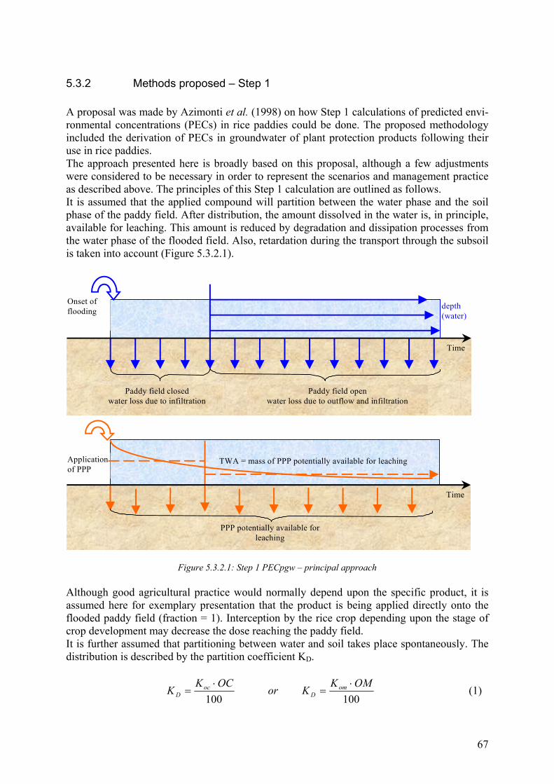
67

5.3.2 Methods proposed – Step 1 A proposal was made by Azimonti et al. (1998) on how Step 1 calculations of predicted envi-ronmental concentrations (PECs) in rice paddies could be done. The proposed methodology included the derivation of PECs in groundwater of plant protection products following their use in rice paddies. The approach presented here is broadly based on this proposal, although a few adjustments were considered to be necessary in order to represent the scenarios and management practice as described above. The principles of this Step 1 calculation are outlined as follows. It is assumed that the applied compound will partition between the water phase and the soil phase of the paddy field. After distribution, the amount dissolved in the water is, in principle, available for leaching. This amount is reduced by degradation and dissipation processes from the water phase of the flooded field. Also, retardation during the transport through the subsoil is taken into account (Figure 5.3.2.1).

Time

Paddy field closedwater loss due to infiltration

Paddy field openwater loss due to outflow and infiltration

Onset offlooding depth

(water)

Time

PPP potentially available forleaching

Applicationof PPP

TWA = mass of PPP potentially available for leaching

Figure 5.3.2.1: Step 1 PECpgw – principal approach Although good agricultural practice would normally depend upon the specific product, it is assumed here for exemplary presentation that the product is being applied directly onto the flooded paddy field (fraction = 1). Interception by the rice crop depending upon the stage of crop development may decrease the dose reaching the paddy field. It is further assumed that partitioning between water and soil takes place spontaneously. The distribution is described by the partition coefficient KD.

100100OMK

KorOCK

K omD

ocD

⋅=

⋅= (1)

68

The mass fraction being re-distributed to the soil phase in the paddy field is then defined by:

dissolvedsorbed

Dsoilwater

waterdissolved

FFand

KBDdepthdepthdepth

F

−=

⋅⋅+=

1 (2)

This leads to the initial paddy water concentration:

dissolvedwater

erceptinitialpw F

depthfDose

PEC ⋅−⋅

⋅=)1(

1.0 int, (3)

For the purpose of assessing the leaching to groundwater, it is reasonable to assume that only the dissolved fraction is available for downward transport whereas the sorbed fraction is re-tained in the upper soil layer. According to common management practice, the paddy field is assumed to be closed for some days after application of the product, thus retaining the water in the field and allowing the product to be effective. Nevertheless, dissipation processes can happen during that period, so that concentrations in the paddy water will decrease. Concentration in the water phase at the end of this water retention period is given by:

pwclose DTtinitialpwcloseendpw ePECPEC 50/)2ln(

,,⋅−

− ⋅= (4) The time weighted average concentration (TWA) during the respective time period (t) is de-fined by:

)2ln(50)1( 50/)2ln(

, ⋅⋅−

⋅=⋅−

close

pwDTt

initialpwpw tDTe

PECTWApwclose

(5)

Finally, the mass of the product available for leaching is derived from the TWA by:

100,

leakagetTWAM closepw

fieldleak

⋅⋅= (6)

Similarly, the decrease in concentration in paddy water during flooding time tflood is calcu-lated. The concentration at the onset of flooding (starting of outflow) is defined by:

closeendpwfloodinitialpw PECPEC −− = ,, (7) The concentration decline during the flooding period is influenced by normal degradation processes on the one hand, but also by the rate of water flowing out of the paddy. This may be described by:

)50

)2ln((

,,

eoutflowratDT

t

floodinitialpwfloodendpwpw

flood

ePECPEC+⋅−

−− ⋅= (8)

69

The outflow rate is calculated from the scenario definition for outflow.

1000000/86400 outfloweoutflowrat ⋅= (9), as there are 86400 s/d and 1000000 L/ha. Finally, again the TWA can be calculated by:

)50

)2ln((

)1()

50)2ln((

,,

eoutflowratDT

t

ePECTWA

pwflood

eoutflowratDT

t

floodinitialpwfloodpw

pwflood

+⋅

−⋅=

+⋅−

− (10)

This leads to the mass of the product potentially available for leaching during the flooding period:

100,

,

leakagetTWAM floodfloodpw

floodleak

⋅⋅= (11)

Potential concentration in paddy groundwater may then be calculated by:

floodleakfieldleakleak MMM ,, += (12) Subsequently, the retardation due to sorption in the soil column and degradation in subsoil layers are considered. The depth of soil is increased to 1m with 3 horizons of 30, 30 and 40 cm. The properties of the different horizons differ in their ability to sorb and degrade pesticides. The differences are based on default assumptions introduced by the FOCUS Ground Water Scenario Workgroup (EC Document Sanco/321/2000) and assume that in the second horizon the OC is 50% of the value of the first horizon (biofactor = 0.5) and in the third horizon it is 30% of the value of the first horizon (biofactor = 0.3). Both sorption and the degradation rate are decreased by these biofactors in the second and third horizons. The adsorption coefficient of each horizon is translated into a retardation coefficient (R). This coefficient defines the difference between the mean residence time of the pesticide compared to that of a conservative tracer (i.e. water). The retardation factor for the first horizon (R1) is given by:

θDKBDR ⋅

+=11 (13)

θ is the volumetric water content of the soil (m3/m3). The value of θ is taken as the saturated volumetric water content of a clayey and a sandy soil type. Corresponding values can be found e.g. in Schaap and Leij (1998). Soil textural classes (USDA) corresponding to the pro-posed scenarios are "clay loam" (Scenario 1) and "sandy loam" (Scenario 2), with correspond-ing saturated volumetric water content of 0.44 and 0.39 for Scenario 1 and Scenario 2, respec-tively. The retardation factor for the second horizon (R2) is given by:

θ5.012

⋅⋅+=

DKBDR (14)

70

The retardation factor for the third horizon (R3) is given by:

θ3.013

⋅⋅+=

DKBDR (15)

The residence time of water in a horizon can be calculated from the leakage rate and the hori-zon depth, given in mm. The residence time of the pesticide (in days) is this residence time multiplied by the retardation coefficient.

leakagedepthRt res

))(

θ⋅⋅= (16)

This residence time is used as the time during which the pesticide degrades in a horizon. The remaining amount of pesticide is then transferred to the next horizon and so on. Finally the amount left in the third horizon in g/ha is translated into a percolate concentration by dividing by the amount of percolate water per year. The mass of pesticide moving from the 0-300mm horizon to the 300 – 600 mm horizon (Mleak(0-300) is therefore given by:

soilres DTtleakleak eMM 50/)2ln(*

*)3000()1(−

=− (17) where Mleak is calculated from equation (11). The mass of pesticide moving from the 300 – 600 mm horizon to the 600 – 1000 mm horizon (Mleak(600-1000)) is given by:

5.0*50/)2ln(**)3000()600300(

)2( soilres DTtleakleak eMM −

−=− (18) and the mass of pesticide moving below the 1000 mm horizon (Mleak(>1000)) is given by:

3.0*50/)2ln(**)600300()1000(

)3( soilres DTtleakleak eMM −

−=> (19)

leakageM

tPEC leakpgw ⋅

⋅== >

365100

)365( )1000( (20)

5.3.3 Proposed model in Step 2 As for surface water a more realistic approach for adsorption is proposed as an intermediate Step 2 in the calculation of the exposure concentration in groundwater. Stefano Cervelli (Cer-velli, 2001) developed also for this situation a proposal that has not yet been thoroughly dis-cussed by the group. In the follow-up group mentioned earlier also this groundwater model will be discussed. The name of the model is MDRICE and the user program CODIWATER also developed by Stefano Cervelli, to calculate the dispersion coefficient necessary in the model (Cervelli, 2001)

71

5.3.4 Available methods – Step 2 and 3

a) Step 2 For step 2 calculations, it is proposed to carry out model calculations using an appropriate leaching model. In the context of the FOCUS (Forum for the Co-ordination of pesticide fate models and their use) work, recommendations were developed concerning the use of such models in the regulatory process (FOCUS (1995)). Currently, regulatory models are limited in their ability to simulate the flooded conditions of a paddy rice field. Also, the hydrology under paddy fields is particularly complex and transient due to the direct interaction between the flooded field, the water-saturated soil and the adja-cent irrigation channels. On the other hand, little was found in the literature about the availability of simulation models capable of the specific hydrology under paddy field conditions. Most of the published model approaches account for leaching only as a potential loss of water (together with evaporation and outflow) and substance. This path is then usually not tracked further down to the ground-water level (see chapter 5.2.3 surface water models, M Vighi et al. (1998)). Therefore, no model in particular can be recommended at the moment for such simulations and further research is needed here. Instead, it is referred to the available regulatory models as recommended by the FOCUS leaching modelling workgroup. The limitations of those need to be kept in mind in the evaluation process. Following principles of good modelling practice, a model should be selected, which does re-flect the relevant processes in a reasonable way. With regard to paddy field conditions, in some aspects only approximations can be achieved due to the complexity involved. Nevertheless, the following should be considered from the hydrological point of view: - Water layer on top of soil and continuous superficial water flow (inflow and outflow) - Evaporation of water from the surface / transpiration by the rice crop - Infiltration into the soil - Transition of unsaturated / saturated conditions in the soil according to water management

practice - Lateral and vertical water flow in the soil, discharge into adjacent surface water bodies. It is considered currently, that the best possible approximation of these processes can be achieved with Richards equation based models. Processes concerning the environmental fate and behaviour of the PPP depend upon the spe-cific compound properties and should be taken into account accordingly. In a recent work of the FOCUS groundwater scenarios workgroup standard scenarios were developed for the purpose of assisting in the establishment of safe uses of PPPs in the context of Annex I inclu-sion (FOCUS, 2000). In relation to that work, it is recommended also for rice products that at this step standard sce-narios should be used for the modelling. Due to the limited and distinct areas of rice growing in Europe, it is considered that two standard scenarios for rice fields would be appropriate to reflect growing conditions in these areas. Soil profiles should be selected in agreement with the above defined soil properties (see chapter 3). A more advanced calculation method may be considered before applying the sophisticated models presented in section 5.3.4. It was not possible for the group to explore this in more detail. In the lack of suitable models for paddy rice conditions a possibility to use PESTLA 3.4 asso-ciated with the model SUSAP 2.07d is described in the SUSAP document on page 36. This possibility could be used on a case by case basis and on expert judgement (Auteri, et al., 2000). In the meantime PEARL has replaced PESTLA.

72

b) Step 3

On a case-by-case basis, further refinement of the leaching model calculations may be re-quired. At this step, modelling should be carried out using site specific or regional data. Leaching assessment at that level may also involve regional groundwater modelling and geo-graphical or statistical approaches where appropriate data is available. 5.4 Soil

5.4.1. Introduction – Tiered Approach Rice culture involves special cropping conditions due to the necessity of a water layer above soil surface for the major part of the crop cycle. This has been described in chapter 2 for the Mediterranean EU member states and two standard scenarios have been proposed in chapter 3 to perform risk assessment at the European level. Plant Protection Products used for rice can be applied to moist, almost water saturated soil after drainage of the paddy field or to the flooded field at different growth stages of the crop. The calculation of PECsoil has to take account of these particular conditions in combination with the proposed scenarios. Similar to the compartments surface water and ground water, a stepwise approach is proposed for the derivation of PECs in soil and the subsequent risk assessment. The proposed approach is illustrated in Figure 5.4.1.1. Step 1 is based on simple assumptions and calculations assuming that the total amount of the applied substance will be distributed in the soil after application to the drained field or that the applied amount will be distributed between the soil and the water phase after application to the flooded field. At Step 2, it is proposed to use simulation models. The models discussed in chapter 5.2.3 (sur-face water) may also be appropriate for calculating soil concentrations, as they generally take into account the partitioning between water and soil or water and sediment phase depending upon the fate and behaviour of the substance under consideration. At Step 3, higher tier testing may be involved. This could include studies in small-scale semi-field outdoor flooded soil systems or full-scale paddy field experiments as discussed in chap-ter 4.1 (data requirements).

73

Figure 5.4.1.1. Stepwise approach for the estimation of the concentration in soil of paddy fields.

Remark: it should be kept in mind that the schemes are just for illustrative purposes and do not represent the full extent of assessment that may be carried out.

yes

no

yes

no

Step 1

Step 2

Soil model calculations for paddyrice scenario

no furtherwork

Step 3

Refined soi l modelling incl. site specificconsiderations and/or geographical /statistical

approaches

PECsoil from spreadsheet calculation1a) wet soil and 1b) flooded

Usesafe?

Usesafe?

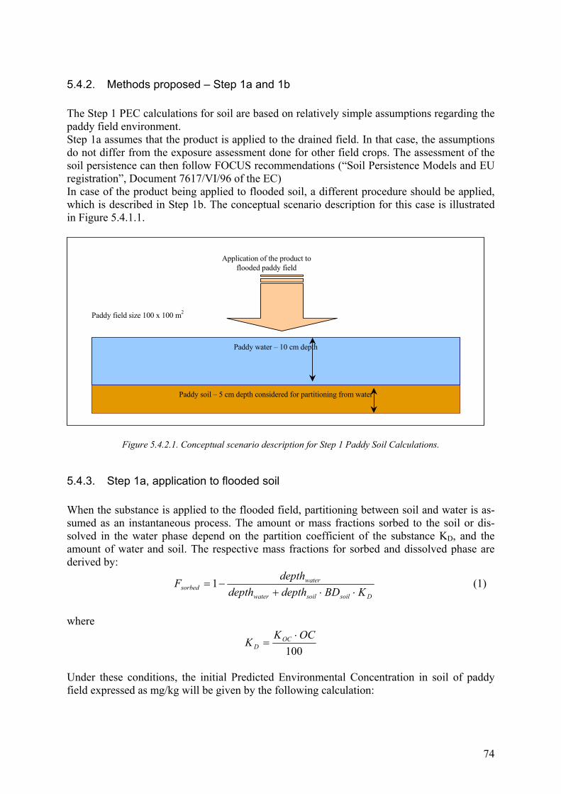
74

5.4.2. Methods proposed – Step 1a and 1b The Step 1 PEC calculations for soil are based on relatively simple assumptions regarding the paddy field environment. Step 1a assumes that the product is applied to the drained field. In that case, the assumptions do not differ from the exposure assessment done for other field crops. The assessment of the soil persistence can then follow FOCUS recommendations (“Soil Persistence Models and EU registration”, Document 7617/VI/96 of the EC) In case of the product being applied to flooded soil, a different procedure should be applied, which is described in Step 1b. The conceptual scenario description for this case is illustrated in Figure 5.4.1.1.

Paddy soil – 5 cm depth considered for partitioning from water

Paddy water – 10 cm depth

Application of the product toflooded paddy field

Paddy field size 100 x 100 m2

Figure 5.4.2.1. Conceptual scenario description for Step 1 Paddy Soil Calculations.

5.4.3. Step 1a, application to flooded soil When the substance is applied to the flooded field, partitioning between soil and water is as-sumed as an instantaneous process. The amount or mass fractions sorbed to the soil or dis-solved in the water phase depend on the partition coefficient of the substance KD, and the amount of water and soil. The respective mass fractions for sorbed and dissolved phase are derived by:

Dsoilsoilwater

watersorbed KBDdepthdepth

depthF

⋅⋅+−= 1 (1)

where

100OCK

K OCD

⋅=

Under these conditions, the initial Predicted Environmental Concentration in soil of paddy field expressed as mg/kg will be given by the following calculation:

75

soilsoil

sorbeddepinitialsoil BDdepth

FDosefPEC

⋅

⋅⋅⋅= 1.0, (2)

Taking into account the degradation in soil (DT50soil), the actual and the time weighted aver-age concentrations in soil can be calculated by the following equations. The DT50soil should be derived from the flooded soil degradation studies or higher tier dissipation studies, where these are available. The actual concentration in soil is given by:

soilDTtinitialsoilsoil ePECtPEC 50/2ln

,)( ⋅−⋅= (3) The time weighted average concentration in soil is calculated by:

soil

DTtinitialsoil

soil DTtePEC

tTWAsoil

50/)2ln()1(

)(50/)2ln(

,

⋅−⋅

=⋅−

(4)

5.4.4. Step 1b, application to drained field When the substance is applied to the drained field, the processes involved do not significantly differ from those relevant for other field crops. In that case, the standard PECsoil calculation used for other crops is proposed. The initial soil concentration can be derived by:

soilsoil

depinitialsoil BDdepth

DosefPEC

⋅

⋅⋅= 1.0, (5)

5.4.5. Step 2, modelling In section 5.2.3, simulation models are discussed which were considered to be appropriate for the modelling of paddy field situations. The models calculate the concentration of the active substance under consideration in the dif-ferent compartments of the model, e.g. water phase, soil or sediment phase, outflow, evapora-tion, leaching, run-off. In addition, the water balance of the system should be in agreement with the water management operations. Thus, the same models may be selected to derive predicted concentrations in soil of the paddy field. For more details refer to section 5.2.3 or the published literature available for these models. A more advanced calculation method may be considered before applying the sophisticated models presented in section 5.2.3. It was not possible for the group to explore this in more detail.

5.4.6. Step 3, site-specific situation. In Step 3 of the estimation of the PEC, refined calculations can be performed taking into ac-count site-specific situations.

76

Refinements may include the results of semi-field or field experiments, the design of which should be based on the requirements described in section 4.1 (data requirements fate and be-haviour). In case of a specific study design, co-operation between the registrant and the re-spective authorities is advisable. Also statistical and / or geographical approaches can be appropriate at this step.

77

6. CONCLUSIONS The following conclusions may be drawn from the work presented here. 1. The workgroup has completed its given task to develop procedures that can be used for

making decisions for the Annex I inclusion of plant protection products used in rice. In order to fulfil this task, the present document was compiled, covering the following as-pects: - agronomic and environmental conditions in rice growing regions in the EU - review and adjustment of the data requirements regarding fate and behaviour in the

environment and ecotoxicology - review of appropriate modelling tools for the estimation of exposure to the environ-

ment by plant protection products used in rice crops. 2. The group has identified the following main areas, which need consideration within the

scope of this guidance document: soil, groundwater, surface water and sediment in the paddy and in the drainage canals. In addition, the ecological function of aquatic organisms within the paddy field should be considered.

3. The review of the cropping conditions in the five Southern EU countries concerned by this

crop has revealed many similarities. The two different standard scenarios proposed repre-sent dominant situations occurring in the MS of concern and offers limited but relevant differences, one based on vulnerable conditions for leaching and the other being more suited to estimate risks in surface waters.

4. Limited changes are proposed in Annex II of Directive 91/414/EEC with regard to the

evaluation of the fate and behaviour of plant protection products in the environment. These affect mainly the test system to be used for investigation of route and rate of degra-dation in soil. It was concluded that an aerobic flooded soil study would be more appro-priate and should replace the normal aerobic soil degradation study. Also, a decision scheme is proposed with regard to the possible necessity of higher tier (e.g. small-scale or full-scale outdoor dissipation) studies. For registration at the national level, relevant regu-latory authority judgement would be required.

5. The major contribution is concerning Annex III. Regarding PEC calculations for soil,

ground waters and surface waters, relevant models for paddy rice conditions have been se-lected on a step 1 purpose for soil and ground waters and up to a step 2 approach for sur-face waters. The specific case of outflow canals has been particularly taken in account. Simple new models or existing more sophisticated ones as RICEWQ have been selected.

6. Environmental fate and behaviour and ecotoxicology requirements have been reviewed

and amended as necessary to account for the specific requirements of rice culture. 7. For ecotoxicological data requirements the workgroup has concluded that current guid-

ance on how to perform the risk assessment for non-target species is acceptable. Aquatic organisms in the rice paddy itself do not require the same level of protection as those in the non-target water bodies adjacent to the fields. However, other species that may use the treated rice paddies as a feeding ground (e.g. birds and mammals) do require the normal

78

level of protection. If specific concerns are identified at national level higher tier studies should be considered on a case by case basis.

8. Currently adopted methods for PEC calculations for surface water, soil, and groundwater

were found to be not fully appropriate for paddy field conditions. Therefore, a stepwise approach has been developed for the estimation of PEC in these compartments after appli-cation of plant protection products in rice. Simple calculation methods for the step 1 as-sessment were developed, which follow partly the current approach for surface water and soil, but deviate from the currently adopted methods for the assessment of leaching to groundwater.

9. Based on current practice separate steps are defined for taking into account degradation

and sorption of the active substance under consideration. 10. Relevant simulation models for paddy rice conditions have been reviewed and proposals

are made for higher tier exposure assessment. Among the readily available simulation models, RICEWQ was considered to be appropriate for the assessment of exposure in sur-face waters. Further research would be needed to fully evaluate the applicability of RI-CEWQ or other models. The model RICEWQ is proposed to be used in connection with RIVWQ model to estimate the PECs in surface waters. RICEMOD may be an appropriate model if more information on it becomes available.

11. Currently, regulatory models to predict groundwater contamination are limited in their

ability to simulate the flooded conditions of a paddy rice field. Thus no model can be rec-ommended at this stage for such simulations and further research is required. If models recommended by the FOCUS leaching modelling workgroup are used the limitations of those need to be kept in mind in the evaluation process. Nevertheless, to take into account the specific hydrological aspects of the rice culture it is currently considered that the best approximations can be achieved with Richards’ equation based models.

12. The development of specific leaching models for rice paddies will give the possibility for

refining PECsoil estimates. 13. In summary, keeping the presentation of the Directive, a document simple to read and to

consult in order to prepare a dossier for EU registration purposes was produced. The method followed has been fully presented for clarity of the options retained in this inte-grated approach. This choice intends also to help both Companies and Authorities if a sci-entific difficulty arises in the preparation of a dossier to evaluate how far the problem to solve deviates from the proposals of the Working Group.

14. The work of the Group is considered a good compromise between an evident lack of sci-

entific information regarding the requirements in the domain of environment and an ur-gent need of guidance for registration purpose at EU level. The present guidance docu-ment is aimed at providing a tool for the regulatory decisions needed. Present proposals could be improved in the near future for EU registration and more urgently if used also for national registration purposes.

79

7. RECOMMENDATIONS As recommendations in the near future attention should be given to the following topics. 1) The difference in sophistication between the relative simple methods proposed and the

more advanced models inventoried may be considered quite large. An in between model-ling method may be incorporated based on the proposals based on the work of Stefano Cervelli (Cervelli, 2001).

2) To obtain the model RICEWQ and RIVWQ for further development as the model to be

used for the assessment of the PEC in surface water after application of plant protection products in rice. Co-operation with USEPA may show very profitable. A working visit may be appropriate.

3) To apply the model when required for the evaluation of active substances to be applied in

rice cultures. 4) To further gain experience with the model and possible to start a validation project with

the model chosen. 5) As already mentioned in the conclusion, some improvements could be already proposed,

considering the potential loss of active substance and / or relevant metabolites from the paddy water to the atmosphere.

6) The group did not yet find a solution for an appropriate risk assessment for micro-

organisms as is indicated in section 4.2.2 under point 8.5 and 10.7. Future scientific de-velopments in the area should be awaited.

7) The development of a step 3 model should be considered by the Southern European coun-

tries for the further risk assessment at higher tiers with respect to the estimation of PECs. Several models for the different environmental compartments may be taken into account for further development.

8) The definition of specific scenarios for higher tier risk assessment may be considered

compared to the European scenarios for ground and surface water. 9) National scenarios may be developed by the Southern European Member States to evalu-

ate the active substances applied in rice on the national level.

80

REFERENCES 1. ACPA website (2000): http://www.acpa.org/public/issues/em/em-apnb1.html 2. Auteri D., Brenna S., Capri E., Paracchini R., Riparbelli C., Trevisan M. (2000). SuSAP

"Allestimento di uno strumento innovativo di supporto alle autorita locali e agli operatori agricoli per una produzione agricola sostenibile". Progetto LIFE-Ambiante 98/ENV/IT/000010. Manuale metodologico. 89p.

3. Azimonti, G.; Alfarroba, F.; Oliveira, B. & Linders, J. (1998). Scenario Development for

Registration of Plant Protection Products in Rice. Poster presented at the 9th IUPAC Con-gress on Pesticide Chemistry, London, 2 – 7 August 1998.

4. Batalla J.A., (1994). Las malas hierbas y su control en el cultivo del arroz. Phytoma

España. nº 63.96-107. 5. Borrero A. (1997). Cultivo del arroz en las marismas del Guadalquivir. 17-29. En Cultivo

del arroz en clima mediterraneo. Junta de Andalucia. CAP 2/97. 6. Carretero J.L. 1987. Rice flora and vegetation in the provinces of Valencia y Tarragona.

Collectanea Botánica. 17(1), 1987. 7. Centre Français du Riz (Mas du Sonnailler, 13200 Arles, France). Soil analysis. Not pub-

lished. 8. Cervelli (2001). Personal communication. 9. Charizopoulos and Papadopoulou-Mourkidou, (1999). A monitoring study carried out in

the most important rice area, the Axios River Basin. 10. Danos, D. (2000). Institute of Wheat (NAGREF), personal communication. 11. ESCORT 2, (2001) Guidance document on regulatory testing and risk assessment proce-

dures for plant protection products with non-target arthropods. Eds.: M.P. Candolfi, K.L. Barrett, P.J. Campbell et.al. SETAC/ESCORT2 Workshop Report, 21-23 March 2000, Wageningen, The Netherlands.

12. Ferrero, A. and Tabacchi, M. (2000). L’ottimizzazione del diserbo del riso. Atti Convegno

“Il controllo della flora infestante: un esempio di ottimizzazione a vantaggio dell’ambiente e della produzione”, Milano, December 5-6, pp. 111-149.

13. Ferrero, A., Tabacchi, M. and Vidotto, F. (1999). Italian rice field weeds and their control.

In 2nd Temperate Rice Conference, Sacramento, California, USA, June 13-17, in press. 14. FOCUS (1995). Pesticide leaching models and EU registration. European Commission

Document 4952/VI/95.

81

15. FOCUS (1996a). Surface Water Models and EU Registration of Plant Protection Products. European Commission Document 6476/VI/1996.

16. FOCUS (1996b). Soil Persistence Models and EU Registration. European Commission

Document 7617/VI/1996. 17. FOCUS (2000). FOCUS groundwater scenarios in the EU plant protection product review

process. Report of the FOCUS groundwater scenarios workgroup, EC Document Refer-ence Sanco/321/2000. 197 pp.

18. FOCUS (2001). “FOCUS Surface Water Scenarios in the EU Evaluation Process under

91/414/EEC”. Report of the FOCUS Working Group on Surface Water Scenarios, EC Document Reference SANCO/4802/2001-rev.2. 245 pp.

19. Greppi. M., Silvestri, S., Anselmetti, M.P., Vietti, L., and Raviola, F. (1998). Giornata

mondiale dell’acqua, Roma, Italy. 20. Heurteaux P. (1996). L’eau et la riziculture en Camargue. Not published. This report is

available at CFR, Mas du Sonnailler, 13200 Arles, France. 21. Hirosji Tsuchida and Tatsuo Katou (1992). Mathematical model of Pollution Caused by

Aerial Application of Pesticides to Rice Fields. Chemosphere, Vol. 24, No. 7, pp 867-879, 1992. See the extended summary in Pestic. Sci. 1997, 49, 210-212.

22. Hosang, J., (1999). Optimierung des Einsatzes eines Herbizids in Reisfeldern mittels

Computersimulation. Presentation of RICEMOD by J. Hosang. 23. Inao, K. & Kitamura, Y. (1999). Pesticide Paddy Field Model (PADDY) for Predicting

Pesticide Concentrations in Water and Soil in Paddy Fields. Pestic. Sci., Vol. 55, pp. 38-46.

24. Kiefer, E. (1999). Exposure Assessment of Surface Waters after Treatment of (flooded)

Rice Paddy Field with Crop Protection Products. Lecture presented during Workshop on Environmental Risk Parameters for Use of Plant Protection Products in Rice, Cremona, I, 16 September 1999.

25. Linders, J & F. Alfarroba (2001), Mathematical Modelling of Pesticides Applied in Rice,

Report to the MED-Rice working Group, Brussels, 9 February 2001, 22 pp. 26. Machado, C. (1999) - Some Considerations on Rice Crop - Direcção-Geral de Protecção

das Culturas, Ministério da Agricultura, do Desenvolvimento Rural e das Pescas. Oeiras. 27. OECD (2002a). OECD Guideline for the Testing of Chemicals, Aerobic and Anaerobic

Transformation in Soil. OECD Test Guideline 307, OECD, Paris. May 2002. 28. OECD(2002a). OECD Guideline for the Testing of Chemicals, Aerobic and Anaerobic

Transformation in Aquatic Sediment Systems. OECD Test Guideline 308, OECD, Paris. May 2002.

82

29. Pereira, H. F. (1997) - Balanço Hidrológico em Canteiros de arroz. Trabalho de fim de curso de Engenharia Agrícola. Universidade de Évora, Évora.

30. Pereira, H. F.; Serralheiro, R.; Pereira, R. (2000) - O Balanço Hidrológico em Canteiros

de arroz. Aspectos ambientais da Cultura. Rev. de Ciências Agrárias Vol. XXIII, Nº 1. 31. Pereira, T.; Cerejeira, M.J.; Brito, F.; Viana, P. (2000) – Exposição e Efeitos de Pesticidas

em Águas Superficiais de Ecosistemas Orizícolas (1998-2000). Instituto Superior de Agronomia/Direcção Geral do Ambiente, Lisboa.

32. Ramos, F. M. et al. (1985) – Projecto de Desenvolvimento Agrícola do Baixo Mondego.

Relatório da Carta de Solos. Direcção Geral de Hidráulica e Engenharia Agrícola, Minis-tério da Agricultura.

33. SANCO (2000). Guidance document on risk assessment for birds and mammals -

SANCO/4145/2000 Available on the web site of DG SANCO: http://www.europa.eu.int/comm/food/fs/ph_ps/pro/wrkdoc/index_en.htm

34. SANCO (2001). Guidance Document on Aquatic Ecotoxicology - SANCO/3268/2001

rev.4 (final) Available on the web site of DG SANCO: http://www.europa.eu.int/comm/food/fs/ph_ps/pro/wrkdoc/index_en.htm

35. SANCO (2002). Guidance Document on Terrestrial Ecotoxicology - SANCO/10329/2002

rev 2 final. Available on the web site of DG SANCO: http://www.europa.eu.int/comm/food/fs/ph_ps/pro/wrkdoc/index_en.htm

36. Schaap, M.G., and F.J. Leij (1998). Database Related Accuracy and Uncertainty of Pe-

dotransfer Functions, Soil Science 163:765-779. 37. Takagi, K.; Fajardo, F.F.; Inao, K. and Kitamura, Y. (1998). Predicting Pesticide Behav-

iour in Lowland Environment using Computer Simulation. Reviews in Toxicology, Vol. 2, pp. 269-286.

38. Vighi, M.; D Sandroni and C Sbriscia Fioretti (1996). Modelling herbicide fate in paddy

fields. X Symposium Pesticide Chemistry, Piacenza.

83

APPENDICES Manual for using the Appendices. In the Appendices A – D EXCEL-sheets are given, with which it is possible to perform the calculations for Step 1 of the exposure assessment of plant protection products applied in rice paddies. To use the EXCEL-sheets as intended the user should proceed as follows (an implicit assumption is that the programme EXCEL is available on the PC):

1) start WORD on the PC, open the MED-Rice report and place the cursor in cell A1 with the content ‘1’;

2) start EXCEL with a new and empty sheet, place the cursor in cell A1; 3) insert a fourth worksheet with the command: Insert, Worksheet; 4) name sheet 4: ‘Input’ by double clicking on Sheet4 and typing ‘Input’; 5) name sheet 1: ‘PEC sw pw’ by double clicking on Sheet1 and typing ‘PEC sw

pw’; 6) name sheet 2: ‘PEC sed soil’ by double clicking on Sheet2 and typing ‘PEC sed

soil’; 7) name sheet 3: ‘PEC gw’ by double clicking on Sheet3 and typing ‘PEC gw’; 8) adjust in sheet ‘Input’ the column width of the columns A – G to 5, 42, 16, 1, 1, 1,

16, respectively by moving the vertical column separator to the required width; 9) adjust in sheet ‘PEC sw pw’ the column width of the columns A – G to 5, 30, 15,

15, 15, 5, 15, respectively by moving the vertical column separator to the required width;

10) adjust in sheet ‘PEC sed soil’ the column width of the columns A – G to 5, 30, 15, 15, 15, 5, 15, respectively by moving the vertical column separator to the required width;

11) adjust in sheet ‘PEC gw’ the column width of the columns A – G to 5, 36, 15, 3, 3, 3, 15, respectively by moving the vertical column separator to the required width;

12) Return to WORD and place the cursor on ‘Substance’, cell B1 of the page ‘Expla-nation of calculations in sheet Input data’ (page 85). Please note, do not use page 84;

13) Mark all the cells from B1 – C50 and press ‘Copy’; 14) Return to EXCEL and paste these cells in sheet ‘Input’, cell B1; 15) Return to WORD and mark the cells under ‘G’ not including the letter ‘G’ itself

and press ‘Copy’ again; 16) Return to EXCEL and paste these cells in sheet ‘Input’, cell G1; 17) ‘Centre’ the columns C – G; 18) If you want to check the text in the document with the formulas of the EXCEL-

sheets, press simultaneously the keys ‘Control’ and ‘`’ (backward accent); 19) Pressing this key-combination again and you will return to the sheet showing the

values instead of the formulas; 20) Move forward to sheet ‘PEC sw pw’; 21) Return to WORD and repeat the marking, copying and pasting procedure for all

the appropriate ranges of the tables for the sheet ‘PEC sw pw’; 22) Repeat the same procedure for the sheets ‘PEC sed soil’ and ‘PEC gw’.

Remark 1: Make sure, that you only copy and paste when you are in the ‘formulas’-mode. Remark 2: Please note, that the figures are not automatically adjusted. Remark 3: To run the standard scenarios for another a.i. change only the yellow (grey) data.

84

A. Example Input Data for EXCEL sheets

A B C D E F G 1 SUBSTANCE: Testcompound 2 3 INPUT: Scenario data I Scenario 1 Scenario 2 4 Soil texture clayey sandy 5 OC soil (%) 1,8 0,9 6 7 depth water (m) (water level in field) 0,1 0,1 8 Water velocity: 9 field (L/sec/ha) 3 3

10 outflow (L/sec/ha) 0,5 0,5 11 Leakage (mm/d) (infiltration rate) 1 10 12 13 t close (d) (time of closure of field) 5 5 14 t flood (d) (time of flooding) 120 120 15 16 depth canal (m) (deepness of outflow) 1 1 17 18 INPUT: Scenario data II 19 area (m2) (area of rice field) 10000 10000 20 Volume of water in field (L) 1000000 1000000 21 22 depth soil (m) 0,05 0,05 23 BD soil (kg/dm3) (soil bulk density) 1,5 1,5 24 25 Outflow rate (1/d) 0,0432 0,0432 26 Dilution factor 10 10 27 28 depth sediment (m) (active sediment depth) 0,05 0,05 29 OC (%) of sediment 1,6 1,6 30 BD sediment (kg/dm3) (sediment bulk density) 1,5 1,5 31 32 INPUT: Product 33 Dose (g/ha) (application rate of product) 100 100 34 35 f dep (fraction of dose deposited to paddy field) 1 1 36 f drift (fraction drift to adjacent water body) 0,0277 0,0277 37 38 Koc (dm3/kg) 10 100 39 Kd (soil) (dm3/kg) 0,18 0,9 40 Kd (sediment) (dm3/kg) 0,16 1,6 41 F sorbed (soil) (fraction partitioning to soil) 0,119 0,403 42 F sorbed (sediment) (fraction partitioning to sediment) 0,012 0,107 43 44 DT50 total,pw (d) in flooded soil system 3 3 45 DT50 pw (d) in water phase 3 3 46 DT50 soil (d) in solid phase 3 3 47 48 DT50 total,sw (d) in sediment/water system 3 3 49 DT50 sw (d) in water phase 3 3 50 DT50 sed (d) in solid phase 3 3

85

Explanation of calculations in sheet Input data:

A B C 1 SUBSTANCE: Test compound 2 3 INPUT: Scenario data I Scenario 1 4 Soil texture clayey 5 OC soil (%) 1,8 6 7 depth water (m) (water level in field) 0,1 8 Water velocity: 9 field (L/sec/ha) 3

10 outflow (L/sec/ha) 0,5 11 Leakage (mm/d) (infiltration rate) 1 12 13 t close (d) (time of closure of field) 5 14 t flood (d) (time of flooding) 120 15 16 depth canal (m) (deepness of outflow) 1 17 18 INPUT: Scenario data II 19 area (m2) (area of rice field) 10000 20 Volume of water in field (L) =$C$19*$C$7*1000 21 22 depth soil (m) 0,05 23 BD soil (kg/dm3) (soil bulk density) 1,5 24 25 Outflow rate (1/d) =$C$10*60*60*24/$C$20 26 Dilution factor 10 27 28 depth sediment (m) (active sediment depth) 0,05 29 OC (%) of sediment 1,6 30 BD sediment (kg/dm3) (sediment bulk density) 1,5 31 32 INPUT: Product 33 Dose (g/ha) (application rate of product) 100 34 35 f dep (fraction of dose deposited to paddy field) 1 36 f drift (fraction drift to adjacent water body) 0,0277 37 38 Koc (dm3/kg) 10 39 Kd (soil) (dm3/kg) =$C$38*$C$5/100 40 Kd (sediment) (dm3/kg) =$C$38*$C$29/100 41 F sorbed (soil) (fraction partitioning to soil) =1-$C$7/($C$7+$C$39*$C$22*$C$23) 42 F sorbed (sediment) (fraction partitioning to sediment) =1-$C$16/($C$16+$C$40*$C$28*$C$30) 43 44 DT50 total,pw (d) in flooded soil system 3 45 DT50 pw (d) in water phase 3 46 DT50 soil (d) in solid phase 3 47 48 DT50 total,sw (d) in sediment/water system 3 49 DT50 sw (d) in water phase 3 50 DT50 sed (d) in solid phase 3

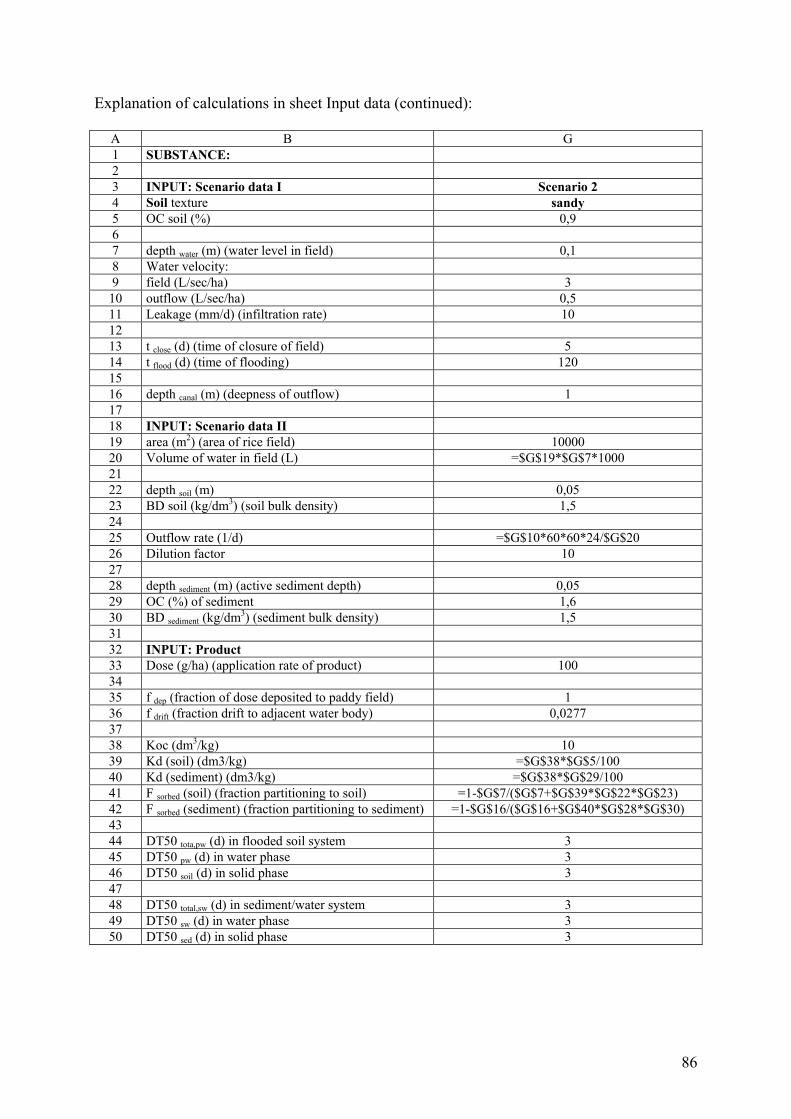
86

Explanation of calculations in sheet Input data (continued):

A B G 1 SUBSTANCE: 2 3 INPUT: Scenario data I Scenario 2 4 Soil texture sandy 5 OC soil (%) 0,9 6 7 depth water (m) (water level in field) 0,1 8 Water velocity: 9 field (L/sec/ha) 3

10 outflow (L/sec/ha) 0,5 11 Leakage (mm/d) (infiltration rate) 10 12 13 t close (d) (time of closure of field) 5 14 t flood (d) (time of flooding) 120 15 16 depth canal (m) (deepness of outflow) 1 17 18 INPUT: Scenario data II 19 area (m2) (area of rice field) 10000 20 Volume of water in field (L) =$G$19*$G$7*1000 21 22 depth soil (m) 0,05 23 BD soil (kg/dm3) (soil bulk density) 1,5 24 25 Outflow rate (1/d) =$G$10*60*60*24/$G$20 26 Dilution factor 10 27 28 depth sediment (m) (active sediment depth) 0,05 29 OC (%) of sediment 1,6 30 BD sediment (kg/dm3) (sediment bulk density) 1,5 31 32 INPUT: Product 33 Dose (g/ha) (application rate of product) 100 34 35 f dep (fraction of dose deposited to paddy field) 1 36 f drift (fraction drift to adjacent water body) 0,0277 37 38 Koc (dm3/kg) 10 39 Kd (soil) (dm3/kg) =$G$38*$G$5/100 40 Kd (sediment) (dm3/kg) =$G$38*$G$29/100 41 F sorbed (soil) (fraction partitioning to soil) =1-$G$7/($G$7+$G$39*$G$22*$G$23) 42 F sorbed (sediment) (fraction partitioning to sediment) =1-$G$16/($G$16+$G$40*$G$28*$G$30) 43 44 DT50 tota,pw (d) in flooded soil system 3 45 DT50 pw (d) in water phase 3 46 DT50 soil (d) in solid phase 3 47 48 DT50 total,sw (d) in sediment/water system 3 49 DT50 sw (d) in water phase 3 50 DT50 sed (d) in solid phase 3

87

B. EXCEL sheet for PEC in Surface Water excluding Sediment A1 B C D E G H I 2 RESULTS: Step 1a Scenario 1 Scenario 2 3 PEC pw, initial (mug/L) 100,0000 100,0000 4 PEC sw, drift, initial (mug/L) 0,277 0,277 5 PEC sw, initial (mug/L) 9,3427 9,3427 6 7 RESULTS: Step 1b 8 PEC pw (t close) (mug/L) 31,4980 89,0899 9 PEC sw, drift (t close) (mug/L) 0,0872 0,2468 10 PEC sw (t close) (mug/L) 2,9428 2,9428 11 12 RESULTS: Step 1c 13 PEC pw, initial (mug/L) 88,1057 59,7015 14 PEC sw, drift, initial (mug/L) 0,2737 0,2473 15 16 PEC pw (t close) (mug/L) 27,7516 53,1880 17 PEC sw, drift (t close) (mug/L) 0,0862 0,2203 18 19 PEC sw (t close) (mug/L) 2,6012 2,7608 20 21 PECsw (t) (mug/L) 22 Day PECsw (t) TWAsw (t) PECsw (t) TWAsw (t) 23 0 2,6012 2,7608 24 1 2,0646 1 day 2,3226 2,1912 1 day 2,4650 25 2 1,6387 2 day 2,0830 1,7392 2 day 2,2108 26 4 1,0323 4 day 1,6976 1,0956 4 day 1,8017 27 7 0,5162 7 day 1,2892 0,5478 7 day 1,3683 28 14 0,1024 14 day 0,7725 0,1087 14 day 0,8199 29 21 0,0203 21 day 0,5319 0,0216 21 day 0,5645 30 28 0,0040 28 day 0,4015 0,0043 28 day 0,4261 31 42 0,0002 42 day 0,2680 0,0002 42 day 0,2845 32 50 0,0000 50 day 0,2252 0,0000 50 day 0,2390 33 100 0,0000 100 day 0,1126 0,0000 100 day 0,1195

88

A B C D E G H I 53 PECpw (t) (mug/L) 54 Day PECpw (t) TWA pw (t) PECpw (t) TWA pw (t) 55 0 88,1057 93,6768 56 1 69,9296 1 day 78,6680 74,3513 1 day 83,6423 57 2 55,5031 2 day 70,5534 59,0127 2 day 75,0146 58 4 34,9648 4 day 57,4996 37,1757 4 day 61,1354 59 7 17,4824 7 day 43,6663 18,5878 7 day 46,4274 60 14 3,4689 14 day 26,1654 3,6883 14 day 27,8199 61 21 0,6883 21 day 18,0167 0,7319 21 day 19,1559 62 28 0,1366 28 day 13,5978 0,1452 28 day 14,4576 63 42 0,0054 42 day 9,0787 0,0057 42 day 9,6528 64 50 0,0008 50 day 7,6265 0,0009 50 day 8,1087 65 100 0,0000 100 day 3,8133 0,0000 100 day 4,0544

Step 1 - PEC surface water - Scenario 2

00,5

11,5

22,5

3

0 20 40 60 80 100 120

Time (days)

Con

cent

ratio

n (m

ug/L

)

PEC(t) TWAC(t)

Step 1 - PEC surface water - Scenario 1

0

0,5

1

1,5

2

2,5

3

0 20 40 60 80 100 120

Time (days)

Con

cent

ratio

n (m

ug/L

)

PEC(t) TWAC(t)

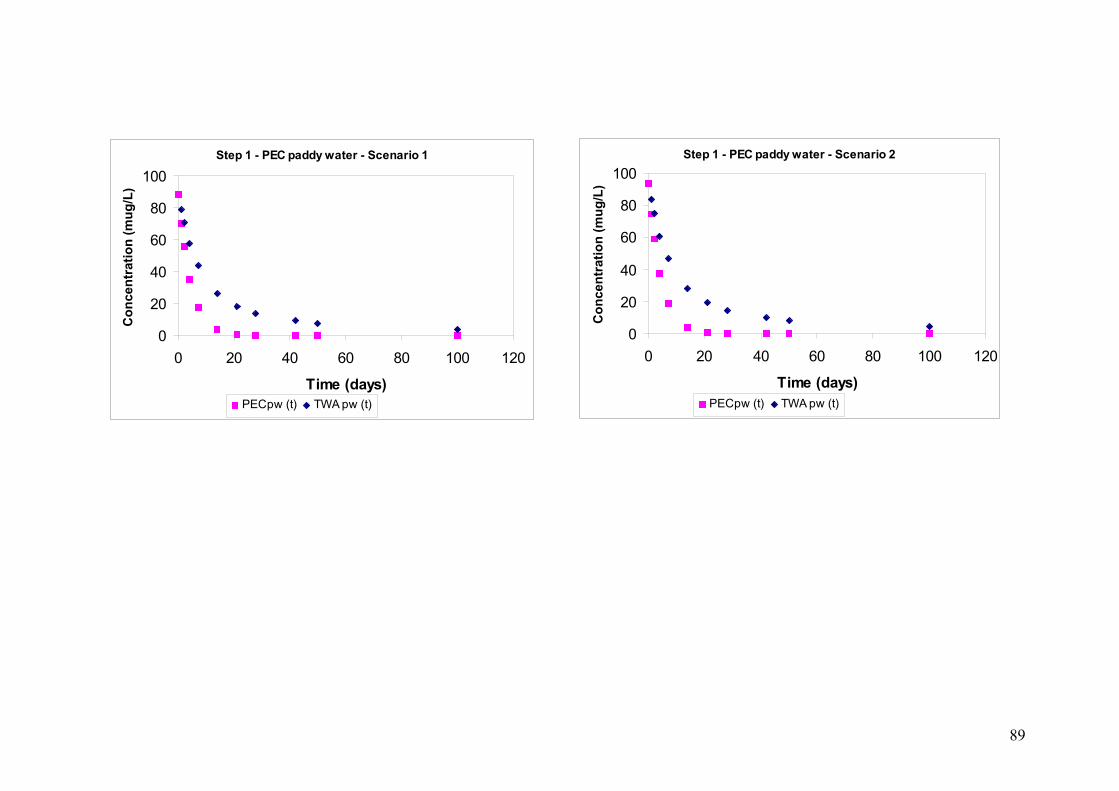
89

Step 1 - PEC paddy water - Scenario 2

0

20

40

60

80

100

0 20 40 60 80 100 120

Time (days)

Con

cent

ratio

n (m

ug/L

)

PECpw (t) TWA pw (t)

Step 1 - PEC paddy water - Scenario 1

0

20

40

60

80

100

0 20 40 60 80 100 120

Time (days)

Con

cent

ratio

n (m

ug/L

)

PECpw (t) TWA pw (t)

90

Explanation of calculations in sheet Surface Water A1 B C 2 RESULTS: Step 1a Scenario 1 3 PEC pw, initial (mug/L) =Input!$C$33*Input!$C$35/Input!$C$7*0,1 4 PEC sw, drift, initial (mug/L) =Input!$C$33*Input!$C$36/Input!$C$16*0,1 5 PEC sw, initial (mug/L) =($C$4*Input!$C$26+'PEC sw pw'!$C$3)/(1+Input!$C$26) 6 7 RESULTS: Step 1b 8 PEC pw (t close) (mug/L) =Input!$C$33*Input!$C$35/Input!$C$7*0,1*EXP(-Input!$C$13*LN(2)/Input!$C$45) 9 PEC sw, drift (t close) (mug/L) =Input!$C$33*Input!$C$36/Input!$C$16*0,1*EXP(-Input!$C$13*LN(2)/Input!$C$49) 10 PEC sw (t close) (mug/L) =($C$9*Input!$C$26+$C$8)/(1+Input!$C$26) 11 12 RESULTS: Step 1c 13 PEC pw, initial (mug/L) =Input!$C$33*Input!$C$35/Input!$C$7*0,1*(1-Input!$C$41) 14 PEC sw, drift, initial (mug/L) =Input!$C$33*Input!$C$36/Input!$C$16*0,1*(1-Input!$C$42) 15 16 PEC pw (t close) (mug/L) =$C$13*EXP(-Input!$C$13*LN(2)/Input!$C$45) 17 PEC sw, drift (t close) (mug/L) =$C$14*EXP(-Input!$C$13*LN(2)/Input!$C$49) 18 19 PEC sw (t close) (mug/L) =($C$17*Input!$C$26+$C$16)/(1+Input!$C$26) 20 21 PECsw (t) (mug/L) 22 Day PECsw (t) 23 0 =$C$19 24 1 =$C$23*EXP(-$B$24*LN(2)/Input!$C$49) 25 2 =$C$23*EXP(-$B$25*LN(2)/Input!$C$49) 26 4 =$C$23*EXP(-$B$26*LN(2)/Input!$C$49) 27 7 =$C$23*EXP(-$B$27*LN(2)/Input!$C$49) 28 14 =$C$23*EXP(-$B$28*LN(2)/Input!$C$49) 29 21 =$C$23*EXP(-$B$29*LN(2)/Input!$C$49) 30 28 =$C$23*EXP(-$B$30*LN(2)/Input!$C$49) 31 42 =$C$23*EXP(-$B$31*LN(2)/Input!$C$49) 32 50 =$C$23*EXP(-$B$32*LN(2)/Input!$C$49) 33 100 =$C$23*EXP(-$B$33*LN(2)/Input!$C$49)

91

Explanation of calculations in sheet Surface Water (continued) A1 D E 2 3 4 5 6 7 8 9 10 11 12 13 14 15 16 17 18 19 20 21 22 TWAsw (t) 23 24 1 day =$C$23*(1-EXP(-$B$24*LN(2)/Input!$C$49))*Input!$C$49/$B$24/LN(2) 25 2 day =$C$23*(1-EXP(-$B$25*LN(2)/Input!$C$49))*Input!$C$49/$B$25/LN(2) 26 4 day =$C$23*(1-EXP(-$B$26*LN(2)/Input!$C$49))*Input!$C$49/$B$26/LN(2) 27 7 day =$C$23*(1-EXP(-$B$27*LN(2)/Input!$C$49))*Input!$C$49/$B$27/LN(2) 28 14 day =$C$23*(1-EXP(-$B$28*LN(2)/Input!$C$49))*Input!$C$49/$B$28/LN(2) 29 21 day =$C$23*(1-EXP(-$B$29*LN(2)/Input!$C$49))*Input!$C$49/$B$29/LN(2) 30 28 day =$C$23*(1-EXP(-$B$30*LN(2)/Input!$C$49))*Input!$C$49/$B$30/LN(2) 31 42 day =$C$23*(1-EXP(-$B$31*LN(2)/Input!$C$49))*Input!$C$49/$B$31/LN(2) 32 50 day =$C$23*(1-EXP(-$B$32*LN(2)/Input!$C$49))*Input!$C$49/$B$32/LN(2) 33 100 day =$C$23*(1-EXP(-$B$33*LN(2)/Input!$C$49))*Input!$C$49/$B$33/LN(2)

92

Explanation of calculations in sheet Surface Water (continued) A1 B G 2 RESULTS: Step 1a Scenario 2 3 PEC pw, initial (mug/L) =Input!$G$33*Input!$G$35/Input!$G$7*0,1 4 PEC sw, drift, initial (mug/L) =Input!$G$33*Input!$G$36/Input!$G$16*0,1 5 PEC sw, initial (mug/L) =($G$4*Input!$G$26+'PEC sw pw'!$G$3)/(1+Input!$G$26) 6 7 RESULTS: Step 1b 8 PEC pw (t close) (mug/L) =Input!$G$33*Input!$G$35/Input!$G$7*0,1*EXP(-Input!$G$13*LN(2)/Input!$G$45) 9 PEC sw, drift (t close) (mug/L) =Input!$G$33*Input!$G$36/Input!$G$16*0,1*EXP(-Input!$G$13*LN(2)/Input!$G$49) 10 PEC sw (t close) (mug/L) =($G$9*Input!$G$26+$G$8)/(1+Input!$G$26) 11 12 RESULTS: Step 1c 13 PEC pw, initial (mug/L) =Input!$G$33*Input!$G$35/Input!$G$7*0,1*(1-Input!$G$41) 14 PEC sw, drift, initial (mug/L) =Input!$G$33*Input!$G$36/Input!$G$16*0,1*(1-Input!$G$42) 15 16 PEC pw (t close) (mug/L) =$G$13*EXP(-Input!$G$13*LN(2)/Input!$G$45) 17 PEC sw, drift (t close) (mug/L) =$G$14*EXP(-Input!$G$13*LN(2)/Input!$G$49) 18 19 PEC sw (t close) (mug/L) =($G$17*Input!$G$26+$G$16)/(1+Input!$G$26) 20 21 PECsw (t) (mug/L) 22 Day PECsw (t) 23 0 =$G$19 24 1 =$G$23*EXP(-$B$24*LN(2)/Input!$G$49) 25 2 =$G$23*EXP(-$B$25*LN(2)/Input!$G$49) 26 4 =$G$23*EXP(-$B$26*LN(2)/Input!$G$49) 27 7 =$G$23*EXP(-$B$27*LN(2)/Input!$G$49) 28 14 =$G$23*EXP(-$B$28*LN(2)/Input!$G$49) 29 21 =$G$23*EXP(-$B$29*LN(2)/Input!$G$49) 30 28 =$G$23*EXP(-$B$30*LN(2)/Input!$G$49) 31 42 =$G$23*EXP(-$B$31*LN(2)/Input!$G$49) 32 50 =$G$23*EXP(-$B$32*LN(2)/Input!$G$49) 33 100 =$G$23*EXP(-$B$33*LN(2)/Input!$G$49)

93

Explanation of calculations in sheet Surface Water (continued) A1 H I 2 3 4 5 6 7 8 9 10 11 12 13 14 15 16 17 18 19 20 21 22 TWAsw 23 24 1 day =$G$23*(1-EXP(-$B$24*LN(2)/Input!$G$49))*Input!$G$49/$B$24/LN(2) 25 2 day =$G$23*(1-EXP(-$B$25*LN(2)/Input!$G$49))*Input!$G$49/$B$25/LN(2) 26 4 day =$G$23*(1-EXP(-$B$26*LN(2)/Input!$G$49))*Input!$G$49/$B$26/LN(2) 27 7 day =$G$23*(1-EXP(-$B$27*LN(2)/Input!$G$49))*Input!$G$49/$B$27/LN(2) 28 14 day =$G$23*(1-EXP(-$B$28*LN(2)/Input!$G$49))*Input!$G$49/$B$28/LN(2) 29 21 day =$G$23*(1-EXP(-$B$29*LN(2)/Input!$G$49))*Input!$G$49/$B$29/LN(2) 30 28 day =$G$23*(1-EXP(-$B$30*LN(2)/Input!$G$49))*Input!$G$49/$B$30/LN(2) 31 42 day =$G$23*(1-EXP(-$B$31*LN(2)/Input!$G$49))*Input!$G$49/$B$31/LN(2) 32 50 day =$G$23*(1-EXP(-$B$32*LN(2)/Input!$G$49))*Input!$G$49/$B$32/LN(2) 33 100 day =$G$23*(1-EXP(-$B$33*LN(2)/Input!$G$49))*Input!$G$49/$B$33/LN(2)

94

Explanation of calculations in sheet Surface Water (continued)

A B C 53 PECpw (t) (mug/L) 54 day PECpw (t) 55 0 =$C$13 56 1 =$C$55*EXP(-$B$56*LN(2)/Input!$C$45) 57 2 =$C$55*EXP(-$B$57*LN(2)/Input!$C$45) 58 4 =$C$55*EXP(-$B$58*LN(2)/Input!$C$45) 59 7 =$C$55*EXP(-$B$59*LN(2)/Input!$C$45) 60 14 =$C$55*EXP(-$B$60*LN(2)/Input!$C$45) 61 21 =$C$55*EXP(-$B$61*LN(2)/Input!$C$45) 62 28 =$C$55*EXP(-$B$62*LN(2)/Input!$C$45) 63 42 =$C$55*EXP(-$B$63*LN(2)/Input!$C$45) 64 50 =$C$55*EXP(-$B$64*LN(2)/Input!$C$45) 65 100 =$C$55*EXP(-$B$65*LN(2)/Input!$C$45)

A D E 53 54 TWApw (t) 55 56 1 day =$C$55*(1-EXP(-$B$56*LN(2)/Input!$C$45))*Input!$C$45/$B$56/LN(2) 57 2 day =$C$55*(1-EXP(-$B$57*LN(2)/Input!$C$45))*Input!$C$45/$B$57/LN(2) 58 4 day =$C$55*(1-EXP(-$B$58*LN(2)/Input!$C$45))*Input!$C$45/$B$58/LN(2) 59 7 day =$C$55*(1-EXP(-$B$59*LN(2)/Input!$C$45))*Input!$C$45/$B$59/LN(2) 60 14 day =$C$55*(1-EXP(-$B$60*LN(2)/Input!$C$45))*Input!$C$45/$B$60/LN(2) 61 21 day =$C$55*(1-EXP(-$B$61*LN(2)/Input!$C$45))*Input!$C$45/$B$61/LN(2) 62 28 day =$C$55*(1-EXP(-$B$62*LN(2)/Input!$C$45))*Input!$C$45/$B$62/LN(2) 63 42 day =$C$55*(1-EXP(-$B$63*LN(2)/Input!$C$45))*Input!$C$45/$B$63/LN(2) 64 50 day =$C$55*(1-EXP(-$B$64*LN(2)/Input!$C$45))*Input!$C$45/$B$64/LN(2) 65 100 day =$C$55*(1-EXP(-$B$65*LN(2)/Input!$C$45))*Input!$C$45/$B$65/LN(2)

95

Explanation of calculations in sheet Surface Water (continued)

A B G 53 PECpw (t) (mug/L) 54 Day PECpw

55 0 =$G$13 56 1 =$G$55*EXP(-$B$56*LN(2)/Input!$G$45) 57 2 =$G$55*EXP(-$B$57*LN(2)/Input!$G$45) 58 4 =$G$55*EXP(-$B$58*LN(2)/Input!$G$45) 59 7 =$G$55*EXP(-$B$59*LN(2)/Input!$G$45) 60 14 =$G$55*EXP(-$B$60*LN(2)/Input!$G$45) 61 21 =$G$55*EXP(-$B$61*LN(2)/Input!$G$45) 62 28 =$G$55*EXP(-$B$62*LN(2)/Input!$G$45) 63 42 =$G$55*EXP(-$B$63*LN(2)/Input!$G$45) 64 50 =$G$55*EXP(-$B$64*LN(2)/Input!$G$45) 65 100 =$G$55*EXP(-$B$65*LN(2)/Input!$G$45)

A H I 53 54 TWApw 55 56 1 day =$G$55*(1-EXP(-$B$56*LN(2)/Input!$G$45))*Input!$G$45/$B$56/LN(2) 57 2 day =$G$55*(1-EXP(-$B$57*LN(2)/Input!$G$45))*Input!$G$45/$B$57/LN(2) 58 4 day =$G$55*(1-EXP(-$B$58*LN(2)/Input!$G$45))*Input!$G$45/$B$58/LN(2) 59 7 day =$G$55*(1-EXP(-$B$59*LN(2)/Input!$G$45))*Input!$G$45/$B$59/LN(2) 60 14 day =$G$55*(1-EXP(-$B$60*LN(2)/Input!$G$45))*Input!$G$45/$B$60/LN(2) 61 21 day =$G$55*(1-EXP(-$B$61*LN(2)/Input!$G$45))*Input!$G$45/$B$61/LN(2) 62 28 day =$G$55*(1-EXP(-$B$62*LN(2)/Input!$G$45))*Input!$G$45/$B$62/LN(2) 63 42 day =$G$55*(1-EXP(-$B$63*LN(2)/Input!$G$45))*Input!$G$45/$B$63/LN(2) 64 50 day =$G$55*(1-EXP(-$B$64*LN(2)/Input!$G$45))*Input!$G$45/$B$64/LN(2) 65 100 day =$G$55*(1-EXP(-$B$65*LN(2)/Input!$G$45))*Input!$G$45/$B$65/LN(2)

96

C. EXCEL sheet for PEC in Soil and Sediment A1 B C D E G H I 2 Scenario 1 Scenario 2 3 4 5 6 7 8 9 10 11 12 RESULTS: Step 1c 13 PEC soil, initial (mug/kg) 15,8590 8,4309 14 PEC sed, drift, initial (mug/kg) 0,0438 0,0438 15 16 PEC soil (t close) (mug/kg) 4,9953 2,6556 17 PEC sed, drift (t close) (mug/kg) 0,0138 0,0138 18 19 PEC sed (t close) (mug/kg) 0,4526 0,4803 20 21 PECsed (t) (mug/kg) 22 Day PECsed (t) TWAsed (t) PECsed (t) TWAsed (t) 23 0 0,4526 0,4803 24 1 0,3592 1 day 0,4041 0,3812 1 day 0,4288 25 2 0,2851 2 day 0,3624 0,3026 2 day 0,3846 26 4 0,1796 4 day 0,2953 0,1906 4 day 0,3135 27 7 0,0898 7 day 0,2243 0,0953 7 day 0,2380 28 14 0,0178 14 day 0,1344 0,0189 14 day 0,1426 29 21 0,0035 21 day 0,0925 0,0038 21 day 0,0982 30 28 0,0007 28 day 0,0698 0,0007 28 day 0,0741 31 42 0,0000 42 day 0,0466 0,0000 42 day 0,0495 32 50 0,0000 50 day 0,0392 0,0000 50 day 0,0416 33 100 0,0000 100 day 0,0196 0,0000 100 day 0,0208

97

A B C D E G H I 53 PECsoil (t) (mug/kg) 54 Day PECsoil TWAsoil PECsoil TWAsoil

55 0 15,8590 8,4309 56 1 12,5873 1 day 14,1602 6,6916 1 day 7,5278 57 2 9,9906 2 day 12,6996 5,3111 2 day 6,7513 58 4 6,2937 4 day 10,3499 3,3458 4 day 5,5022 59 7 3,1468 7 day 7,8599 1,6729 7 day 4,1785 60 14 0,6244 14 day 4,7098 0,3319 14 day 2,5038 61 21 0,1239 21 day 3,2430 0,0659 21 day 1,7240 62 28 0,0246 28 day 2,4476 0,0131 28 day 1,3012 63 42 0,0010 42 day 1,6342 0,0005 42 day 0,8687 64 50 0,0002 50 day 1,3728 0,0001 50 day 0,7298 65 100 0,0000 100 day 0,6864 0,0000 100 day 0,3649

Step 1 - PEC sediment - Scenario 2

0,00000,10000,20000,30000,40000,50000,6000

0 20 40 60 80 100 120

Time (days)

Con

cent

ratio

n (m

ug/k

g)

PECsed (t) TWAsed (t)

Step 1 - PEC sediment - Scenario 1

0,0000

0,1000

0,2000

0,3000

0,4000

0,5000

0 20 40 60 80 100 120

Time (days)

Con

cent

ratin

(mug

/kg)

PECsed (t) TWAsed (t)

98

Step 1 - PEC soil - Scenario 2

0,0000

2,0000

4,0000

6,0000

8,0000

10,0000

0 20 40 60 80 100 120

Time (days)

Con

cent

ratio

n (m

ug/k

g)

PECsoil (t) TWAsoil (t)

Step 1 - PEC soil - Scenario 1

0,0000

5,0000

10,0000

15,0000

20,0000

0 20 40 60 80 100 120

Time (days)

Con

cent

ratin

(mug

/kg)

PECsoil (t) TWAsoil (t)

99

Explanation of calculations in sheet Soil and Sediment: A1 B C 2 Scenario 1 3 4 5 6 7 8 9 10 11 12 RESULTS: Step 1c 13 PEC soil, initial (mug/kg) =Input!$C$33*Input!$C$35*Input!$C$41/Input!$C$22/Input!$C$23*0,1 14 PEC sed, drift, initial (mug/kg) =Input!$C$33*Input!$C$36*Input!$C$42/Input!$C$28/Input!$C$30*0,1 15 16 PEC soil (t close) (mug/kg) =$C$13*EXP(-Input!$C$13*LN(2)/Input!$C$46) 17 PEC sed, drift (t close) (mug/kg) =$C$14*EXP(-Input!$C$13*LN(2)/Input!$C$50) 18 19 PEC sed (t close) (mug/kg) =$C$17+'PEC sw pw'!$C$16*Input!$C$16*Input!$C$42/Input!$C$26/Input!$C$28/Input!$C$30 20 21 PECsed (t) (mug/kg) 22 Day PECsed 23 0 =$C$19 24 1 =$C$23*EXP(-$B$24*LN(2)/Input!$C$50) 25 2 =$C$23*EXP(-$B$25*LN(2)/Input!$C$50) 26 4 =$C$23*EXP(-$B$26*LN(2)/Input!$C$50) 27 7 =$C$23*EXP(-$B$27*LN(2)/Input!$C$50) 28 14 =$C$23*EXP(-$B$28*LN(2)/Input!$C$50) 29 21 =$C$23*EXP(-$B$29*LN(2)/Input!$C$50) 30 28 =$C$23*EXP(-$B$30*LN(2)/Input!$C$50) 31 42 =$C$23*EXP(-$B$31*LN(2)/Input!$C$50) 32 50 =$C$23*EXP(-$B$32*LN(2)/Input!$C$50) 33 100 =$C$23*EXP(-$B$33*LN(2)/Input!$C$50)

100

Explanation of calculations in sheet Soil and Sediment (continued): A1 B C 2 3 4 5 6 7 8 9 10 11 12 13 14 15 16 17 18 19 20 21 22 TWAsed 23 24 1 day =$C$23*(1-EXP(-$B$24*LN(2)/Input!$C$50))*Input!$C$50/$B$24/LN(2) 25 2 day =$C$23*(1-EXP(-$B$25*LN(2)/Input!$C$50))*Input!$C$50/$B$25/LN(2) 26 4 day =$C$23*(1-EXP(-$B$26*LN(2)/Input!$C$50))*Input!$C$50/$B$26/LN(2) 27 7 day =$C$23*(1-EXP(-$B$27*LN(2)/Input!$C$50))*Input!$C$50/$B$27/LN(2) 28 14 day =$C$23*(1-EXP(-$B$28*LN(2)/Input!$C$50))*Input!$C$50/$B$28/LN(2) 29 21 day =$C$23*(1-EXP(-$B$29*LN(2)/Input!$C$50))*Input!$C$50/$B$29/LN(2) 30 28 day =$C$23*(1-EXP(-$B$30*LN(2)/Input!$C$50))*Input!$C$50/$B$30/LN(2) 31 42 day =$C$23*(1-EXP(-$B$31*LN(2)/Input!$C$50))*Input!$C$50/$B$31/LN(2) 32 50 day =$C$23*(1-EXP(-$B$32*LN(2)/Input!$C$50))*Input!$C$50/$B$32/LN(2) 33 100 day =$C$23*(1-EXP(-$B$33*LN(2)/Input!$C$50))*Input!$C$50/$B$33/LN(2)

101

Explanation of calculations in sheet Soil and Sediment (continued): A1 B G 2 RESULTS: Step 1a Scenario 2 3 PEC pw, initial (mug/L) 4 PEC sw, drift, initial (mug/L) 5 PEC sw, initial (mug/L) 6 7 RESULTS: Step 1b 8 PEC pw (t close) (mug/L) 9 PEC sw, drift (t close) (mug/L) 10 PEC sw (t close) (mug/L) 11 12 RESULTS: Step 1c 13 PEC pw, initial (mug/L) =Input!$G$33*Input!$G$35*Input!$G$41/Input!$G$22/Input!$G$23*0,1 14 PEC sw, drift, initial (mug/L) =Input!$G$33*Input!$G$36*Input!$G$42/Input!$G$28/Input!$G$30*0,1 15 16 PEC pw (t close) (mug/L) =$G$13*EXP(-Input!$G$13*LN(2)/Input!$G$46) 17 PEC sw, drift (t close) (mug/L) =$G$14*EXP(-Input!$G$13*LN(2)/Input!$G$50) 18 19 PEC sw (t close) (mug/L) =$G$17+'PEC sw pw'!$G$16*Input!$G$16*Input!$G$42/Input!$G$26/Input!$G$28/Input!$G$30 20 21 PECsw (t) (mug/L) 22 Day PECsed 23 0 =$G$19 24 1 =$G$23*EXP(-$B$24*LN(2)/Input!$G$50) 25 2 =$G$23*EXP(-$B$25*LN(2)/Input!$G$50) 26 4 =$G$23*EXP(-$B$26*LN(2)/Input!$G$50) 27 7 =$G$23*EXP(-$B$27*LN(2)/Input!$G$50) 28 14 =$G$23*EXP(-$B$28*LN(2)/Input!$G$50) 29 21 =$G$23*EXP(-$B$29*LN(2)/Input!$G$50) 30 28 =$G$23*EXP(-$B$30*LN(2)/Input!$G$50) 31 42 =$G$23*EXP(-$B$31*LN(2)/Input!$G$50) 32 50 =$G$23*EXP(-$B$32*LN(2)/Input!$G$50) 33 100 =$G$23*EXP(-$B$33*LN(2)/Input!$G$50)

102

Explanation of calculations in sheet Soil and Sediment (continued): A1 B G 2 3 4 5 6 7 8 9 10 11 12 13 14 15 16 17 18 19 20 21 22 TWAsed 23 24 1 day =$G$23*(1-EXP(-$B$24*LN(2)/Input!$G$50))*Input!$G$50/$B$24/LN(2) 25 2 day =$G$23*(1-EXP(-$B$25*LN(2)/Input!$G$50))*Input!$G$50/$B$25/LN(2) 26 4 day =$G$23*(1-EXP(-$B$26*LN(2)/Input!$G$50))*Input!$G$50/$B$26/LN(2) 27 7 day =$G$23*(1-EXP(-$B$27*LN(2)/Input!$G$50))*Input!$G$50/$B$27/LN(2) 28 14 day =$G$23*(1-EXP(-$B$28*LN(2)/Input!$G$50))*Input!$G$50/$B$28/LN(2) 29 21 day =$G$23*(1-EXP(-$B$29*LN(2)/Input!$G$50))*Input!$G$50/$B$29/LN(2) 30 28 day =$G$23*(1-EXP(-$B$30*LN(2)/Input!$G$50))*Input!$G$50/$B$30/LN(2) 31 42 day =$G$23*(1-EXP(-$B$31*LN(2)/Input!$G$50))*Input!$G$50/$B$31/LN(2) 32 50 day =$G$23*(1-EXP(-$B$32*LN(2)/Input!$G$50))*Input!$G$50/$B$32/LN(2) 33 100 day =$G$23*(1-EXP(-$B$33*LN(2)/Input!$G$50))*Input!$G$50/$B$33/LN(2)

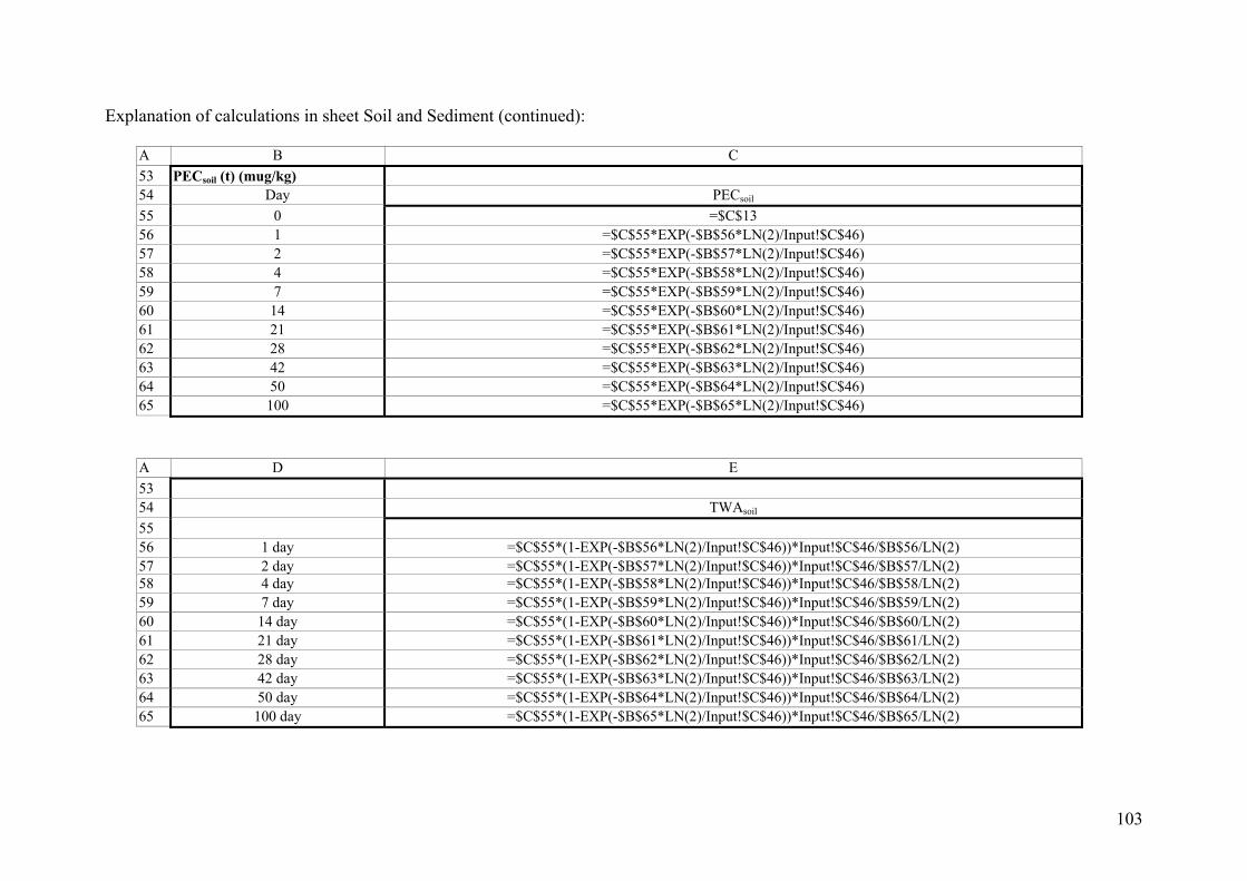
103

Explanation of calculations in sheet Soil and Sediment (continued):

A B C 53 PECsoil (t) (mug/kg) 54 Day PECsoil

55 0 =$C$13 56 1 =$C$55*EXP(-$B$56*LN(2)/Input!$C$46) 57 2 =$C$55*EXP(-$B$57*LN(2)/Input!$C$46) 58 4 =$C$55*EXP(-$B$58*LN(2)/Input!$C$46) 59 7 =$C$55*EXP(-$B$59*LN(2)/Input!$C$46) 60 14 =$C$55*EXP(-$B$60*LN(2)/Input!$C$46) 61 21 =$C$55*EXP(-$B$61*LN(2)/Input!$C$46) 62 28 =$C$55*EXP(-$B$62*LN(2)/Input!$C$46) 63 42 =$C$55*EXP(-$B$63*LN(2)/Input!$C$46) 64 50 =$C$55*EXP(-$B$64*LN(2)/Input!$C$46) 65 100 =$C$55*EXP(-$B$65*LN(2)/Input!$C$46)

A D E 53 54 TWAsoil 55 56 1 day =$C$55*(1-EXP(-$B$56*LN(2)/Input!$C$46))*Input!$C$46/$B$56/LN(2) 57 2 day =$C$55*(1-EXP(-$B$57*LN(2)/Input!$C$46))*Input!$C$46/$B$57/LN(2) 58 4 day =$C$55*(1-EXP(-$B$58*LN(2)/Input!$C$46))*Input!$C$46/$B$58/LN(2) 59 7 day =$C$55*(1-EXP(-$B$59*LN(2)/Input!$C$46))*Input!$C$46/$B$59/LN(2) 60 14 day =$C$55*(1-EXP(-$B$60*LN(2)/Input!$C$46))*Input!$C$46/$B$60/LN(2) 61 21 day =$C$55*(1-EXP(-$B$61*LN(2)/Input!$C$46))*Input!$C$46/$B$61/LN(2) 62 28 day =$C$55*(1-EXP(-$B$62*LN(2)/Input!$C$46))*Input!$C$46/$B$62/LN(2) 63 42 day =$C$55*(1-EXP(-$B$63*LN(2)/Input!$C$46))*Input!$C$46/$B$63/LN(2) 64 50 day =$C$55*(1-EXP(-$B$64*LN(2)/Input!$C$46))*Input!$C$46/$B$64/LN(2) 65 100 day =$C$55*(1-EXP(-$B$65*LN(2)/Input!$C$46))*Input!$C$46/$B$65/LN(2)

104

Explanation of calculations in sheet Soil and Sediment (continued):

A B G 53 PECsoil 54 Day PECsoil

55 0 =$G$13 56 1 =$G$55*EXP(-$B$56*LN(2)/Input!$G$46) 57 2 =$G$55*EXP(-$B$57*LN(2)/Input!$G$46) 58 4 =$G$55*EXP(-$B$58*LN(2)/Input!$G$46) 59 7 =$G$55*EXP(-$B$59*LN(2)/Input!$G$46) 60 14 =$G$55*EXP(-$B$60*LN(2)/Input!$G$46) 61 21 =$G$55*EXP(-$B$61*LN(2)/Input!$G$46) 62 28 =$G$55*EXP(-$B$62*LN(2)/Input!$G$46) 63 42 =$G$55*EXP(-$B$63*LN(2)/Input!$G$46) 64 50 =$G$55*EXP(-$B$64*LN(2)/Input!$G$46) 65 100 =$G$55*EXP(-$B$65*LN(2)/Input!$G$46)

A H I 53 54 TWAsoil

55 56 1 day =$G$55*(1-EXP(-$B$56*LN(2)/Input!$G$46))*Input!$G$46/$B$56/LN(2) 57 2 day =$G$55*(1-EXP(-$B$57*LN(2)/Input!$G$46))*Input!$G$46/$B$57/LN(2) 58 4 day =$G$55*(1-EXP(-$B$58*LN(2)/Input!$G$46))*Input!$G$46/$B$58/LN(2) 59 7 day =$G$55*(1-EXP(-$B$59*LN(2)/Input!$G$46))*Input!$G$46/$B$59/LN(2) 60 14 day =$G$55*(1-EXP(-$B$60*LN(2)/Input!$G$46))*Input!$G$46/$B$60/LN(2) 61 21 day =$G$55*(1-EXP(-$B$61*LN(2)/Input!$G$46))*Input!$G$46/$B$61/LN(2) 62 28 day =$G$55*(1-EXP(-$B$62*LN(2)/Input!$G$46))*Input!$G$46/$B$62/LN(2) 63 42 day =$G$55*(1-EXP(-$B$63*LN(2)/Input!$G$46))*Input!$G$46/$B$63/LN(2) 64 50 day =$G$55*(1-EXP(-$B$64*LN(2)/Input!$G$46))*Input!$G$46/$B$64/LN(2) 65 100 day =$G$55*(1-EXP(-$B$65*LN(2)/Input!$G$46))*Input!$G$46/$B$65/LN(2)

105

D. EXCEL sheet for PEC in Groundwater:

A1 B C D E F G 2 RESULTS: Step 1 Scenario 1 Scenario 2 3 4 PEC pw, initial (mug/L) 88,1057 93,6768 5 6 PEC pw,end-close (mug/L) 27,7516 29,5063 7 TWA pw (mug/L) 52,2436 55,5470 8 M leak, field (g/ha) 2,6122 27,7735 9 10 PEC pw,initial-flood (mug/L) 27,7516 29,5063 11 PEC pw,end-flood (mug/L) 0,0000 0,0000 12 TWA pw, flood (mug/L) 0,8433 0,8966 13 M leak, flood (g/ha) 1,0119 10,7590 14 15 M leak (g/ha) 3,6241 38,5325 16 17 Kd (depth 0 - 0.3 m) 0,1800 0,0900 18 Kd (depth 0.3 - 0.6 m) 0,0900 0,0450 19 Kd (depth 0.6 - 1.0 m) 0,0540 0,0270 20 21 Saturated water content 0,44 0,39 22 23 t (res) (0 - 0.3 m) (d) 213,00 15,75 24 t (res) (0.3 - 0.6 m) (d) 172,50 13,73 25 t (res) (0.6 - 1.0 m) (d) 208,40 17,22 26 27 DT50 soil (0 - 0.3m: 100 %) (d) 3,00 3,00 28 DT50 soil (0.3 - 0.6 m: 50 %) (d) 6,00 6,00 29 DT50 soil (0.6 - 1.0 m: 30 %) (d) 10,00 10,00 30 31 M leak (> 300) (g/ha) 0,0000 1,0126 32 M leak (> 600) (g/ha) 0,0000 0,2074 33 M leak (> 1000) (g/ha) 0,0000 0,0629 34 35 PEC pgw (mug/L) 0,0000 0,0017

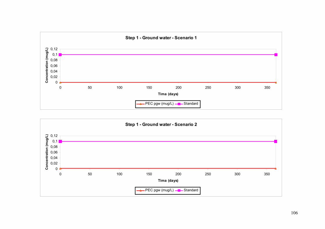
106

Step 1 - Ground water - Scenario 1

00,020,040,060,080,1

0,12

0 50 100 150 200 250 300 350

Tima (days)

Con

cent

ratio

n (m

ug/L

)

PEC pgw (mug/L) Standard

Step 1 - Ground water - Scenario 2

00,020,040,060,080,1

0,12

0 50 100 150 200 250 300 350

Tima (days)

Con

cent

ratio

n (m

ug/L

)

PEC pgw (mug/L) Standard

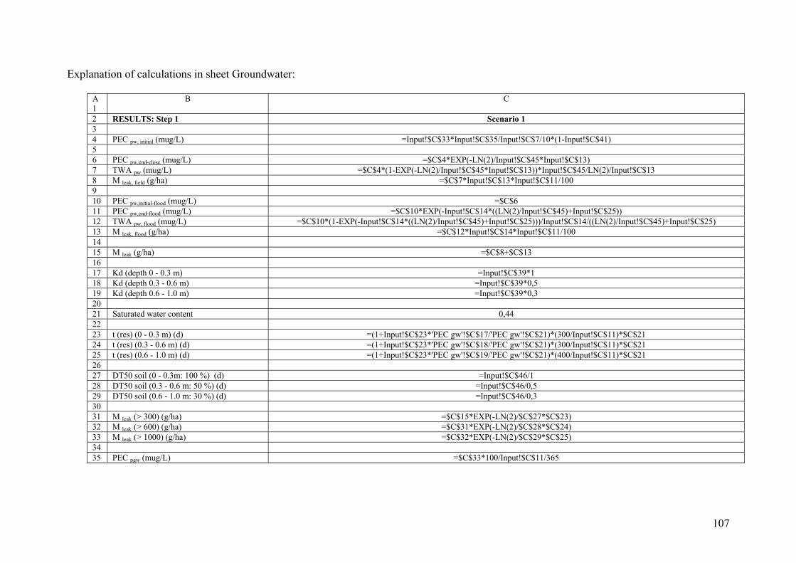
107

Explanation of calculations in sheet Groundwater: A1

B C

2 RESULTS: Step 1 Scenario 1 3 4 PEC pw, initial (mug/L) =Input!$C$33*Input!$C$35/Input!$C$7/10*(1-Input!$C$41) 5 6 PEC pw,end-close (mug/L) =$C$4*EXP(-LN(2)/Input!$C$45*Input!$C$13) 7 TWA pw (mug/L) =$C$4*(1-EXP(-LN(2)/Input!$C$45*Input!$C$13))*Input!$C$45/LN(2)/Input!$C$13 8 M leak, field (g/ha) =$C$7*Input!$C$13*Input!$C$11/100 9 10 PEC pw,initial-flood (mug/L) =$C$6 11 PEC pw,end-flood (mug/L) =$C$10*EXP(-Input!$C$14*((LN(2)/Input!$C$45)+Input!$C$25)) 12 TWA pw, flood (mug/L) =$C$10*(1-EXP(-Input!$C$14*((LN(2)/Input!$C$45)+Input!$C$25)))/Input!$C$14/((LN(2)/Input!$C$45)+Input!$C$25) 13 M leak, flood (g/ha) =$C$12*Input!$C$14*Input!$C$11/100 14 15 M leak (g/ha) =$C$8+$C$13 16 17 Kd (depth 0 - 0.3 m) =Input!$C$39*1 18 Kd (depth 0.3 - 0.6 m) =Input!$C$39*0,5 19 Kd (depth 0.6 - 1.0 m) =Input!$C$39*0,3 20 21 Saturated water content 0,44 22 23 t (res) (0 - 0.3 m) (d) =(1+Input!$C$23*'PEC gw'!$C$17/'PEC gw'!$C$21)*(300/Input!$C$11)*$C$21 24 t (res) (0.3 - 0.6 m) (d) =(1+Input!$C$23*'PEC gw'!$C$18/'PEC gw'!$C$21)*(300/Input!$C$11)*$C$21 25 t (res) (0.6 - 1.0 m) (d) =(1+Input!$C$23*'PEC gw'!$C$19/'PEC gw'!$C$21)*(400/Input!$C$11)*$C$21 26 27 DT50 soil (0 - 0.3m: 100 %) (d) =Input!$C$46/1 28 DT50 soil (0.3 - 0.6 m: 50 %) (d) =Input!$C$46/0,5 29 DT50 soil (0.6 - 1.0 m: 30 %) (d) =Input!$C$46/0,3 30 31 M leak (> 300) (g/ha) =$C$15*EXP(-LN(2)/$C$27*$C$23) 32 M leak (> 600) (g/ha) =$C$31*EXP(-LN(2)/$C$28*$C$24) 33 M leak (> 1000) (g/ha) =$C$32*EXP(-LN(2)/$C$29*$C$25) 34 35 PEC pgw (mug/L) =$C$33*100/Input!$C$11/365

108

Explanation of calculations in sheet Groundwater (continued):

A1

B G

2 RESULTS: Step 1 Scenario 2 3 4 PEC pw, initial (mug/L) =Input!$G$33*Input!$G$35/Input!$G$7/10*(1-Input!$G$41) 5 6 PEC pw,end-close (mug/L) =$G$4*EXP(-LN(2)/Input!$G$45*Input!$G$13) 7 TWA pw (mug/L) =$G$4*(1-EXP(-LN(2)/Input!$G$45*Input!$G$13))*Input!$G$45/LN(2)/Input!$G$13 8 M leak, field (g/ha) =$G$7*Input!$G$13*Input!$G$11/100 9 10 PEC pw,initial-flood (mug/L) =$G$6 11 PEC pw,end-flood (mug/L) =$G$10*EXP(-Input!$G$14*((LN(2)/Input!$G$45)+Input!$G$25)) 12 TWA pw, flood (mug/L) =$G$10*(1-EXP(-Input!$G$14*((LN(2)/Input!$G$45)+Input!$G$25)))/Input!$G$14/((LN(2)/Input!$G$45)+Input!$G$25) 13 M leak, flood (g/ha) =$G$12*Input!$G$14*Input!$G$11/100 14 15 M leak (g/ha) =$G$8+$G$13 16 17 Kd (depth 0 - 0.3 m) =Input!$G$39*1 18 Kd (depth 0.3 - 0.6 m) =Input!$G$39*0,5 19 Kd (depth 0.6 - 1.0 m) =Input!$G$39*0,3 20 21 Saturated water content 0,39 22 23 t (res) (0 - 0.3 m) (d) =(1+Input!$G$23*'PEC gw'!$G$17/'PEC gw'!$G$21)*(300/Input!$G$11)*$G$21 24 t (res) (0.3 - 0.6 m) (d) =(1+Input!$G$23*'PEC gw'!$G$18/'PEC gw'!$G$21)*(300/Input!$G$11)*$G$21 25 t (res) (0.6 - 1.0 m) (d) =(1+Input!$G$23*'PEC gw'!$G$19/'PEC gw'!$G$21)*(400/Input!$G$11)*$G$21 26 27 DT50 soil (0 - 0.3m: 100 %) (d) =Input!$G$46/1 28 DT50 soil (0.3 - 0.6 m: 50 %) (d) =Input!$G$46/0,5 29 DT50 soil (0.6 - 1.0 m: 30 %) (d) =Input!$G$46/0,3 30 31 M leak (> 300) (g/ha) =$G$15*EXP(-LN(2)/$G$27*$G$23) 32 M leak (> 600) (g/ha) =$G$31*EXP(-LN(2)/$G$28*$G$24) 33 M leak (> 1000) (g/ha) =$G$32*EXP(-LN(2)/$G$29*$G$25) 34 35 PEC pgw (mug/L) =$G$33*100/Input!$G$11/365