Embed Size (px)
Citation preview

GUERRILLA DATA ANALYSIS USING MICROSOFT EXCEL
2nd Edition
Oz du Soleil & Bill Jelen
Holy Macro! Books PO Box 82
Uniontown OH 44685

GUERRILLA DATA ANALYSIS USING MICROSOFT EXCEL 2nd Edition
© 2015 Holy Macro! BooksAll rights reserved. No part of this book may be reproduced or transmitted in any form or by any means, electronic or mechanical, including photocopying, recording, or by any information or storage retrieval system without written permission from the publisher.
All terms known in this book known to be trademarks have been appropriately capitalized. Trademarks are the property of their respective owners and are not affiliated with Holy Macro! Books
Every effort has been made to make this book as complete and accurate as possible, but no warranty or fitness is implied. The information is provided on an “as is” basis. The authors and the publisher shall have neither liability nor responsibility to any person or entity with respect to any loss or damages arising from the information contained in this book.
Printed in USA by Hess Print Solutions
First Printing: March 2015
Authors: Oz du Soleil & Bill Jelen
Copy Editor: Kitty Wilson
Indexer: Nellie Jay
Cover Design: Shannon Mattiza, 6Ft4 Productions
Published by: Holy Macro! Books, PO Box 82, Uniontown OH 44685
Distributed by Independent Publishers Group, Chicago, IL
ISBN 978-1-61547-033-4
Library of Congress Control Number: 2014959001
Table of ContentsDedications .........................................................................................................viiAbout the Authors ...............................................................................................vii
Oz du Soleil ........................................................................................................................................................... viiBill Jelen ............................................................................................................................................................... viii
Acknowledgements ............................................................................................viiiIntroduction: Welcome to the World of Guerrilla Data Analysis! ............................x
In The Heat of Conflict .................................................................................................................................. xSmall, Stupid Stuff................................................................................................................................................... xBig, Complicated Stuff ............................................................................................................................................ 1
About This Book and How to Use It ..............................................................................................................1Download the Example Files .........................................................................................................................1
Reviewing the Basics ............................................................................................ 2Overview of Excel Formulas and Functions ...................................................................................................2
Formula Notations .................................................................................................................................................. 2Excel Error Notations .............................................................................................................................................. 3
Changing Formulas to Values ........................................................................................................................3Using Paste Special in Other Ways ................................................................................................................5
Transposing Columns and Rows.............................................................................................................................. 5Performing a Calculation on Every Cell in a Range ................................................................................................. 6
Using Relative, Absolute, and Mixed References ..........................................................................................9Linking Worksheets and Workbooks ...........................................................................................................11
Linking Between Worksheets ............................................................................................................................... 11Linking One Cell to Another on Different Worksheets .......................................................................................... 12Using a VLOOKUP with References to Another Worksheet .................................................................................. 13Inserting Table References Between Worksheets ................................................................................................. 14Linking Workbooks ............................................................................................................................................... 14
Developing Dynamic Spreadsheets ......................................................................15Conditional Formatting ........................................................................................16
Using Conditional Formatting to Make Deadline Alerts ..............................................................................17Using Conditional Formatting to Find Duplicates ........................................................................................19Using Icons with Conditional Formatting ...................................................................................................20
Using IF Statements .............................................................................................22Using an IF Statement with COUNTIF ..........................................................................................................23
Sorting ................................................................................................................24Rules for Sorting ..........................................................................................................................................25
The Data Range Must Be Contiguous (No Empty Rows or Columns) .................................................................... 25Merged Cells Will Not Sort ................................................................................................................................... 27
Using Sorting ...............................................................................................................................................28Using the Quick-Sort Icons .................................................................................................................................... 28Understanding Ascending and Descending Sorts ................................................................................................. 28Sorting with the Aid of a Helper Column .............................................................................................................. 31
What You Need to Know About Filtering Before You Do It ..........................................................................33Let's Start Filtering ......................................................................................................................................33
What’s In the Data Set? ........................................................................................................................................ 34Finding Records Quickly with AutoFilter .....................................................................................................35Filtering to Find the Top (or Bottom) Five Transactions ..............................................................................36Filtering a Date Range Using a Custom AutoFilter ......................................................................................40
Advanced Filter Example 1: Filtering in Place ....................................................................................................... 41Advanced Filter Example 2: OR vs AND Advanced Filtering and Copying to a New Location ...............................42Advanced Filter Example 3: Copying Only Certain Fields to Another Location .....................................................42Advanced Filter Example 4: Filtering Unique Records Only .................................................................................. 43Advanced Filter Example 6: Replacing 362,880 Conditions .................................................................................. 45
Filtering Conclusions ...................................................................................................................................47Using Consolidate ................................................................................................47

iv GUERRILLA DATA ANALYSIS USING MICROSOFT EXCEL
Using Consolidate to Combine Duplicates in Column 1 ..............................................................................47Using Consolidate to Add New Data to Old Data ........................................................................................48
Using Subtotals ...................................................................................................51Copying Only the Subtotals .................................................................................................................................. 52
Adding Additional Subtotals ........................................................................................................................54Warning: Be Careful How You Subtotal! ......................................................................................................55
Summing and Counting Using Criteria ..................................................................58Using SUMIF ................................................................................................................................................58Using SUMIFS and COUNTIFS ......................................................................................................................59Comparing What’s Been Shipped and What’s Been Received ....................................................................61Matching Reps and Rep IDs Using VLOOKUP ..............................................................................................64
VLOOKUP Using TRUE to Assign Grades to Students ............................................................................................ 65Looking Left, Right, and All Around: INDEX and MATCH .............................................................................66
Using INDEX and MATCH ...................................................................................................................................... 66Using INDEX/MATCH/MATCH for a Two-Way Lookup ........................................................................................... 67
Using Pivot Tables................................................................................................68What Is a Pivot Table and What Can It Do? .................................................................................................68
Preview 1: Summing Values with a Pivot Table..................................................................................................... 69Preview 4: Using a Pivot Table to Find a Sum and an Average at the Same Time .................................................70
Creating a Pivot Table ..................................................................................................................................71Summing Values with the Pivot Table ................................................................................................................... 73
Filling Blanks with Zero................................................................................................................................74Counting Values with the Pivot Table ................................................................................................................... 74Filtering Pivot Table Data ...................................................................................................................................... 75Grouping Dates in the Pivot Table ........................................................................................................................ 75Creating a Year-over-Year Report in a Pivot Table ................................................................................................. 78What is the Point of GetPivotData? ...................................................................................................................... 80Using the Pivot Table to Get a Sum & Average at the Same Time ........................................................................ 80Using the Pivot Table to Get the Percentage of the Total ..................................................................................... 81Using the Pivot Table to Filter for the Top Five ..................................................................................................... 82Using the Pivot Table to Drill Down for Isolated Details ....................................................................................... 83Making Many Copies of a Pivot Table ................................................................................................................... 84
Deleting a Pivot Table ..................................................................................................................................85Overriding the Default Row Sequence in a Pivot Table ...............................................................................85Using Calculated Items & Calculated Fields ................................................................................................86
Working with Calculated Items ............................................................................................................................. 86Working with Calculated Fields ...................................................................................................................88
Final Notes on Calculated Items and Calculated Fields......................................................................................... 89Rearranging Pivot Table Headers ................................................................................................................89Pivot Table Q&A ..........................................................................................................................................90Pivot Table Conclusions ...............................................................................................................................92
Using Array Formulas ..........................................................................................92Basic Array Formula ....................................................................................................................................93Copying an Array Formula ...........................................................................................................................94Modifying an Array Formula .......................................................................................................................94Using FREQUENCY to Create a Histogram ...................................................................................................95
Going One Step Further: An Array Inside an Array Formula ................................................................................. 98Array Formulas and System Memory ..........................................................................................................98
Excel Tables: The Glue in Dynamic Spreadsheet Development .............................99Converting a Data Range to a Table ...........................................................................................................99Adding New Data to a Table ......................................................................................................................101Adding a New Column ...............................................................................................................................101Table References and SUMIFS ...................................................................................................................102Using the Table Design Tab .......................................................................................................................103Integrating Tables With Other Excel Features ...........................................................................................103
Mixing Formulas in a Column ............................................................................................................................. 106Adding New Data to a Table ............................................................................................................................... 107Sheet Protection: Tables Must Be Completely Protected or Completely Unprotected. .....................................107

TABLE OF CONTENTS v
Excel Tables Conclusion .............................................................................................................................107The INDIRECT and OFFSET Functions ..................................................................107
Using INDIRECT .........................................................................................................................................107Using INDIRECT to Pick the Worksheet With the Right City ............................................................................... 108Using INDIRECT with VLOOKUP .......................................................................................................................... 109
Using OFFSET .............................................................................................................................................110Using OFFSET to Summarize Data From a Variable Range of Cells ..................................................................... 110
Controlling User Inputs and Data Integrity .........................................................112Data Validation Overview ..........................................................................................................................113Implementing Dropdown Lists ..................................................................................................................113Controlling Dates .......................................................................................................................................114Ensuring Reasonable Numbers .................................................................................................................114Data Validation Conclusions ......................................................................................................................117
Error-Handling and Formula Triggers .................................................................117Error-Handling: show "Discontinued" instead of #N/A .............................................................................118Formula Trigger: Waiting for Complete Information .................................................................................118Error-Handling Functions: IFNA vs. IFERROR .............................................................................................119
Graphing and Charting .......................................................................................119Making a Logarithmic Graph .....................................................................................................................119
Adding Data Labels ............................................................................................................................................. 125Correcting a Chart's Data Range ......................................................................................................................... 126
Playing Around with a Pivot Chart ............................................................................................................130Adding New Data to a Pivot Chart .............................................................................................................131Changing the Chart Type ...........................................................................................................................132Using Slicers with Pivot Charts .................................................................................................................132
One Pivot Chart Horror: automatic refresh will erase your hard work ...............................................................133
Using Slicers ......................................................................................................133Excel 2013: Guerrilla Data Analysis Gets Real .....................................................136
Using Slicers with Tables in Excel 2013......................................................................................................136Data Models and Relationships .................................................................................................................137
Embedding Excel in Web Pages ..........................................................................140Embedding Excel in a Blog Post .................................................................................................................140Differences between Excel Web App and Desktop Excel ..........................................................................143
Down and Dirty Tips and Insights ......................................................................143Forcing a Report to Fit on One Page ..........................................................................................................143Combining Formulas and Text in the Same Cell ........................................................................................144Handling Dates ..........................................................................................................................................146
Correcting Dates That Excel Doesn’t Recognize as Dates ................................................................................... 146Date-Handling Functions .................................................................................................................................... 148Using the TEXT Function with Dates and Times.................................................................................................. 149
Handling Time ...........................................................................................................................................149Understanding Time Formats ............................................................................................................................. 151Converting All Results to Minutes ....................................................................................................................... 151
Unhiding Column A ...................................................................................................................................152Getting Rid of Gridlines .............................................................................................................................152Volatile, Slow, and Peculiar Functions and Features .................................................................................152
Volatile functions and features: .......................................................................................................................... 152Slow-to-Calculate Features and Functions ..................................................................................................152Peculiar Functions ......................................................................................................................................153
Using SUM vs. Adding Individual Cells ......................................................................................................153Useful Excel Functions .......................................................................................154
Using PMT to Predict a Loan Payment ......................................................................................................154Using FORECAST ........................................................................................................................................155Using COUNTA ...........................................................................................................................................155Using RANK ...............................................................................................................................................155

vi GUERRILLA DATA ANALYSIS USING MICROSOFT EXCEL
Using RANK, RANK.EQ, and RANK.AVG............................................................................................................... 155Breaking Ties Based on Position in a List ............................................................................................................ 156Breaking a tie based on number of athletic competitions: ................................................................................. 157
Using CEILING and FLOOR .........................................................................................................................157Using MAX, MIN, LARGE, and SMALL ........................................................................................................158Using CONVERT .........................................................................................................................................158Using ABS to Compare Errors in Absolute Terms ......................................................................................159Using RAND and RANDBETWEEN ..............................................................................................................159
Putting CHOOSE to Work .................................................................................................................................... 162Using SUMPRODUCT .................................................................................................................................163Using EOMONTH .......................................................................................................................................163
Troubleshooting in Excel ....................................................................................164Quickly Checking Sums and Averages .......................................................................................................164Crossfooting ..............................................................................................................................................165Using the Formula Evaluator .....................................................................................................................166Troubleshooting by Checking Highlighted Ranges in a Formula ................................................................167
Spreadsheet Layout and Development ..............................................................168Digging into the Details of the Layout ................................................................................................................ 169Taking Advantage of Good Spreadsheet Layout ................................................................................................. 171Integrating More Data and Making a Pivot Table ............................................................................................... 172
Final Word About Spreadsheet Development ...........................................................................................173Using Keyboard Shortcuts ..................................................................................173
Quickly Navigating Using the Ctrl or End Key .................................................................................................... 173Navigating Between Worksheets ........................................................................................................................ 174Formatting Shortcuts .......................................................................................................................................... 174Clipboard Shortcuts ............................................................................................................................................ 175Calculation Shortcuts .......................................................................................................................................... 175Editing Shortcuts ................................................................................................................................................. 175Excel Commands ................................................................................................................................................. 175F4 Repeats Last Command.................................................................................................................................. 176Using Arrow Keys to Enter a Formula ................................................................................................................. 176
Wrap-Up ............................................................................................................177Index .................................................................................................................179

DEDICATIONS vii
DedicationsTo my mother, Maere Floyd, who seemed like the meanest mother in the world. I’d ask her a question like, “Who was the president when I was born?” Her response would be, “Did you try to look it up?” Eventually, I learned that the only right response was “Yes.” I had to have at least tried.
We had a World Book Encyclopedia set in the living room, and those books were meant for use, not decoration.
All these many years later, that's one lesson has stuck with me and has served me as an analyst, consultant, and Excel power user: If there’s a fact in the world, make an effort to look for it. Don’t make stuff up. Dig, probe, and pick until you get your answer.
As a high school teacher’s aide preparing for retirement, my mother has remained committed to young folks and how they learn. Thanks, Mom!
—Oz du Soleil
To Dan Bricklin, Bob Frankston, and Dan Fylstra.
—Bill Jelen
About the AuthorsOz du Soleil
Biographies tend to be written in the third-person, but let me speak directly to you.
I grew up in the city of North Chicago, Illinois. I joined the US Navy in 1985 and spent six years there. In that time, I served on the fast attack submarine USS Sturgeon (SSN-637) and the fast frigate USS Joseph Hewes (FF-1078).
After the Navy, I graduated from University of Illinois at Chicago (UIC) with a BA in philosophy and a minor in economics and two years of Russian language study. My coursework in philosophy involved logic and decision theory, which offers some insight into my passion for Excel and data—lots of strat-egy, symbols, variables, and parentheses.
I eventually ended up in a job where I used Excel to investigate complaints. Duplicate orders were shipping out, test results weren’t showing up, accounts were assigned to the wrong sales reps, the wrong people were getting termination warning letters. In all those cases, the culprit turned out to be bad data. Some of those problems weren’t mine to solve, but management allowed me to dig into the data, get an understanding of the processes, work with the stakeholders, clean the data, and revise the processes. I loved putting out those fires!
For seven years I put out such fires: uncovering flaws in reports, exposing how calculations in reports didn’t match business rules, modifying processes, cleaning data, and generally reducing the unneces-sary misery caused by crap data.
Today I run a blog, DataScopic.net, that focuses on data and data management, with Excel at the root of it all. After seeing so much data in my own jobs, in working with clients and students, and in discussions with other data folks, my perspective is that Excel is just a tool. We need data-savvy people and solid processes—in addition to the right tools—in order to keep our data clean, and keep termination warning letters from going to the wrong people.

viii GUERRILLA DATA ANALYSIS USING MICROSOFT EXCEL
I love freelancing and taking projects, but I love teaching and speaking even more. That led me to take improv and stand-up comedy courses at Second City. It’s been great and I would recommend it for anyone who regularly gets up in front of people.
During the writing of this book Microsoft awarded me an Excel MVP (Most Valuable Professional) Award. It's given for those who not only show skill, but also contribute to the community. It was a real honor to get the award, and the spirit of community is what fueled the writing of this book.
Thanks for buying this book! I welcome your feedback, at [email protected].
Bill Jelen
I wrote the first edition of this book in 2002. Since then, I have written 44 other books about Microsoft Excel including Pivot Table Data Crunching, Excel Gurus Gone Wild, and Power Excel with MrExcel. You can find 1800 episodes of my Learn Excel podcast on YouTube. My favorite activity is to wow a room full of accountants with my half-day Power Excel seminar. Microsoft has awarded me an Excel MVP award for 10 years. I have run the MrExcel.com website since 1998.
AcknowledgementsThanks to Bill Jelen, Mr. Excel, for the opportunity to write this book, and his leadership in the Excel community.
Thanks to Troy Berry for seeing that I was an analyst before I thought of myself as an analyst. Through his prodding and advice, I began to see this Excel thing as a powerful tool—far more than a fun toy for solving problems.
Thanks to Helena Bouchez for her real-deal coaching that kept me on track and got this book done on time!
Thanks to Keidra Chaney for many many conversations about data and the needs that non-data people have as they are thrust into data-driven roles. Thanks for your shared commitment in empowering those people in understanding the strengths and limitations of data.
Thanks to Monica Johnson, Lupe Miranda, Drew Alexander, and Nancy Migalla. These former co-workers were incredibly supportive not only as co-workers but as teachers who showed me the world of Pivot Tables, the importance of data quality, and that being a good analyst goes beyond the data. There's so much more. It includes managing the people who don’t like the results of the analysis. Being a good analysit also includes being questioned and owning up to it when someone finds mis-takes in your work.
Thanks to Mike “ExcelIsFun” Girvin, Chandoo, Jocelyn and Rob Collie, Szilvia Juhasz, Krisztina Szabó, Maxime Manuel, Kevin Lehrbass, Craig Hatmaker, Petros Chatzipantazis, Rahim Zulfiqar Ali, Mynda Treacy, Ann Emery, Hiran De Silva, and countless others who help make the Excel community support-ive, vibrant, and international—and who remind us why Excel is the number-one business intelligence tool in the world.
Thanks to my fellow co-hosts of Excel TV, Rick Grantham and Jordan Goldmeier, and our wonder-ful Excel TV guests: Zach Barresse, Keidra Chaney, Bill Jelen, Szilvia Juhasz, Kari Finn, Chandoo, Jon Peltier, Mynda Treacy, Johann Odou, John Persico, Mike “ExcelIsFun” Girvin. We’re bringing knowl-edge, insights, fire, and wild adventure to the Excel and data management communities!
Thanks to supporters Patrick Richards, Jeff Bradford, Andreas Pavlatos, Charlie Vlahogiannis, Kate Christenson, Evan Clough, the entire EBassist community, Dave McMillan, Heather Dart, Dianna

ACKNOWLEDGEMENTS ix
Smith, Kelly Casey, Tshombe Brown and too many others to name. I appreciate your passion and interest in seeing this book come to life.
Thanks to Jeff Ashton, the first person who ever told me, “No, there isn’t an Excel feature for that, but here’s a way we can trick Excel into doing it anyway.” To me, that’s when you’re really using Excel—when you’re putting the right formulas and features together to get your work done.
Thanks to Ranjit Souri, my stand-up comedy instructor at Second City, who warned, “You will bomb! You must bomb!” Those eight weeks in Ranjit’s class were a solid lesson that failure is part of any learning process and that you can fail in front of an audience—as long as you’re learning and putting in the work to get better. Analysts do fail in front of others. Good analysts own their mistakes, and fight to get better. Bad analysts end up fired.
Thanks to Andy Crestodina, Amanda Gant, and the Orbiteers Wine & Web events that encourage good, sincere web content. Those events helped give me the opportunity to write this book. In the early days of my blog, when there were no visitors, there was Andy’s quote: “Crickets never hurt anybody.”
Thanks to my clients, who’ve provided the opportunity to help with their data and challenged me with unique needs—stretching my skill and testing Excel’s limits.
Thanks to my workshop students—both public and private—for asking tough questions, being com-mitted to quality data, and wanting to get more out of Excel. And thanks for the feedback that helps me continue to improve as an instructor.
—Oz
Thanks to Oz for rescuing this second edition of Guerilla Data Analysis from the long list of “I will have to do that someday” and making it a reality. When I started reading Oz’s blog and seeing him on Excel TV, it struck me that he was the right guy to carry on the Guerilla Data Analysis franchise.
Thanks to everyone in “row 2” of my seminars.
Thanks to David Gainer, Sam Radakovitz, Ben Rampson, Dan Battigan, Joe Chirilov, Joe Camp, and Kari Finn at Microsoft.
Thanks to Mary Ellen Jelen.
—Bill Jelen

x GUERRILLA DATA ANALYSIS USING MICROSOFT EXCEL
Introduction: Welcome to the World of Guerrilla Data Analysis!Over the years that I’ve been consulting, teaching workshops, and writing a blog, it’s become clear to me that there are a lot of people who are in data-driven roles but don’t have a data background. They aren’t sure what Excel can really do, but spreadsheets keep showing up in their inboxes. One of my students complained that she got a promotion, more money, and the title Social Media Strategist. However, instead of getting more social media activity, she got a mountain of data and was directed to “find something interesting in this.” She had become an unwitting data analyst who didn’t know where to start.
Other students and clients have told stories about taking a week to manually compare lists that were thousands of rows long; retyping data that came to them in ALL CAPS; spending days creating sum-maries while not knowing that Pivot Tables are designed to make those summaries in seconds. This is the world of guerrilla data analysis, where you’re in the heat of data conflict, without formal training, and you need to make something happen.
If you’re reading this, you’re probably a guerrilla analyst, and hopefully you’ll get useful tips and insights from this book, as well as solutions that end unnecessary misery. The examples here are practical and cover a wide variety of areas, including nonprofits, web analytics, accounting, cooking, and retail. The goal is to stimulate ideas by exposing you to the variety of ways to use Excel.
In The Heat of ConflictData is coming from everywhere, about all kinds of things. All the cool kids are talking about big data, data science, and predictive analysis. But data also presents everyday problems that aren’t as glamor-ous as millions of rows of data and Nate Silver coming to tell us the future. Data analysis involves both the small, stupid stuff and big, complicated stuff.
Small, Stupid Stuff
One afternoon in 2005, I needed to print certificates on expensive paper. It was late in the afternoon, and the certificates absolutely had to ship that day. I did the Excel–Word mail merge, and the certifi-cates were coming out of the printer with weirdo numbers instead of dates: 38491, 38464, and 38478 instead of 5/19/2005, 4/22/2005, and 5/6/2005. C’mon! Really?! Now?!
It took me two hours to learn that the Short Date formatting in Excel had been changed to General, and I only had to change it back and redo the merge. But the glitch had already cost me at least 50 sheets of fancy paper, the afternoon was gone, and I’d done a lot of worrying that I’d have to tell a lot of people that the certificates weren’t going to ship on time.
That afternoon I didn’t really have an analysis problem, but my story is a good example of an analyst going into panic mode after all the true hard-core analysis has been done. It’s an example of how small, stupid details can turn a process sideways. Another reason for telling this story is to let you know that you’re not the only one who’s been stopped by small things.
Students ask about these types of disruptions and start their questions with “This may seem like a small thing, but…” It’s not small when you’re under pressure and a whole process has stopped. Guerrilla conflict is guerrilla conflict.

INTRODUCTION: WELCOME TO THE WORLD OF GUERRILLA DATA ANALYSIS! 1
Big, Complicated Stuff
Data analysis involves all kinds of tasks—from investigating known or perceived problems to forecast-ing to developing dashboards to cleaning data to doing financial modeling—while also satisfying the end users.
One of my first, and favorite, freelancing jobs involved supporting a project manager. She was leading the migration of 400 phone systems (with 200 columns of data for each of the 400 rows) and needed a summary page that provided a simple overview. We spent hours together, going over the complex calculation of contract expiration dates, prorated charges, disconnect charges, disconnect dates, con-nection dates, additional fees associated with carrier X but not carriers Y and Z, and fees associated with certain systems. This all had to be right so we could show each of the 400 managers what they would save by migrating early rather than migrating at the deadline, 15 months away.
With extremely complicated formulas, having a strategy is key to getting the calculations right. You can do complex calculations in one big formula, but you end up creating a parentheses torture cham-ber. In devising a calculation strategy, it’s important for an analyst to answer two questions:
● If I have to come back to this in three months, how easily can I figure out what I did? ● If someone else has to figure it out, how easily can that person trace my thinking?
Breaking complicated calculations into pieces, using helper columns, and creating lookup grids will help build those complex calculations and make it easier (for the original analyst or someone else) to troubleshoot later.
About This Book and How to Use ItExcel has many features, and every analyst has different needs. So, rather than providing an Excel A-to-Z, this book moves in a rapid-fire way, assuming that you have some basic level of Excel skill. You can read straight through the book or, you can use it as a reference, when you have an immediate challenge or simply wonder, “Is there a better way?”
Most sections of this book are short and designed to give quick insight with practical examples.
Some images do not show the entire data sets because they're too large. In those situations, if you want to see the full set, the examples workbooks are available for download
Here's a secret: In a few of the example workbooks there are extras that are labeled BONUS and aren't covered in this book. These bonus examples were sometimes too elaborate, and scrapped for something more focused. Still, they were worth at least sharing with those of you who are interested.
Download the Example FilesIf you would like to work along with any example in this book, you can download the spreadsheets at:
http://www.datascopic.net/gdav2-downloads

2 GUERRILLA DATA ANALYSIS USING MICROSOFT EXCEL
Reviewing the BasicsThis book assumes that you have some basic knowledge of Excel. However, even seasoned Excel veterans miss some of the basics, so let’s start with some fundamentals that will serve you well when you’re working with data and things get hot.
Overview of Excel Formulas and FunctionsThere is a difference between a formula and a function. Formulas start with = and do not always use a function.
=3+2 is a formula without a function.
=B3+E3 is a formula without a function, and it adds the values in cells B3 and E3.
SUM is a function.
=SUM(3,2,11) is a formula with the SUM function, and would add 3+2+11.
=B1*MAX(A3:C20) is a formula that uses MAX to find the maximum value in the range A3:C20 and multiplies that result by the value in cell B1.
Therefore, functions are those features in Excel that are named like MAX, COUNTA, SUMIFS, NOW, TAN, KURT, CHAR, etc, and they are programmed to perform specific tasks.
There are hundreds of Excel functions, grouped in 11 categories. No one has reason to memorize every function. Instead, getting the most from Excel requires using resources like online forums, tuto-rials, books, and just asking people if they can help answer questions.
The following tables show some of the ways that Excel communicates with its users via formula nota-tion and error messages.
Formula Notations
Here is a list of some of the notation that you’ll see in formulas and what they mean.

REVIEWING THE BASICS 3
Excel Error Notations
Here is a list of some of the errors that you’ll see in Excel and what they mean.
Changing Formulas to ValuesHere’s a must-know: You should always get rid of formulas if they’ve done their job and are no longer needed.
Say that you’ve received a report that has the first and last names in separate cells and you need the full names in one cell.
To get the names put together, you can use the & symbol to concatenate them:
In this figure, notice the formula =A2&” “&B2. You have to include the space between the first and last names. (To see for yourself, set up a similar spreadsheet and use the formula =A2&B2 instead.)

4 GUERRILLA DATA ANALYSIS USING MICROSOFT EXCEL
Once you have the names in one cell, you’re done with columns A and B. But can you just delete them? Nope! If you delete the columns, you get a #REF! error because the formulas are looking for data that no longer exists:
t
You need to undo the deletion with Ctrl+Z and get your data back.
To do this right, you have to get rid of the formulas in column C before you can delete the data in columns A and B. There are several ways to do this. Here’s one:
1. Highlight the range that contains underlying formulas and right-click.2. In the context menu that pops up, select Copy and then select Paste As Values, which is desig-
nated by the clipboard icon with the 123, as shown in the image below.
Now the formulas are gone. You have actual data in the Full Name column, and you’re free to delete the First Name and Last Name columns.
If your keyboard has an Application key (which looks like a mouse cursor pointing to a dropdown menu and is often between the right Alt and Ctrl keys), you can convert to values by pressing Ctrl+C and then pressing and releasing the Application key and then pressing the V key.
You don’t have an Application key?
Here’s yet another way to paste as values after you’ve copied the original data:1. On the Home tab, select the arrow at the bottom of the Clipboard group.2. In the menu that appears, select Paste Special to open the Paste Special dialog. Notice in the
figure below that Values is selected in the Paste section.

REVIEWING THE BASICS 5
3. Click OK to get rid of the formulas in the Full Name column, leaving only the data.
Using Paste Special in Other WaysThe Paste Special options in Excel are worth getting to know. You’ve seen how to use Paste Special to change formulas to values. The following sections cover two more features: Transpose and, Multiply.
Transposing Columns and Rows
For one thing, you can use Paste Special to transpose columns and rows. Say that you have city names as column headers, as shown in the next figure, but you’d rather work with them as row headers.
Here’s what you do:1. Highlight the range and press Ctrl+C (or right-click and select Copy) to copy it.2. Select the cell where you want the vertical data to start. The following figure shows the cursor
in cell A4.
3. On the Home tab, select the arrow at the bottom of the Paste icon. From the menu that appears, select Paste Special to open the Paste Special dialog.
4. Select the Transpose check box, as shown in the following figure. Click OK.

6 GUERRILLA DATA ANALYSIS USING MICROSOFT EXCEL
Excel makes the cities into row headers instead of column headers—and it transposes the corre-sponding data into the right place, too.
Performing a Calculation on Every Cell in a Range
Say that you have a range of 48 cells that represent sales data, and you need to calculate a revenue share amount of 14% on each of the 48 cells. You can use Paste Special for this, too, and here’s how you do it:
1. Enter 0.14 in an empty cell (G2 in the image below).2. Press Ctrl+C (or right-click the cell and select Copy) to copy it.3. Highlight the range of 48 cells of sales data, right-click, and select Paste Special.4. In the Paste Special dialog, select the Multiply radio button and then click OK.

REVIEWING THE BASICS 7
5. Excel did the multiplication for you but it’s also changed the formatting to General.
With the cells still highlighted, Select Home | Accounting | click the dollar-sign to convert the General format to Accounting.
TIP:Choose both Values and Multiply in the Paste Special dialog to preserve the original number
formats in the paste range.
Using Helper ColumnsUsing helper columns isn’t actually an Excel feature, but it’s a really great strategy for dealing with complex formulas. When you need multiple calculations in a formula, you can break the actions into several steps or multiple formulas rather than try to write a massive formula all at once.
Say that you have a list of employees, along with the pay rate for each, the number of hours each employee has worked, and the number of overtime hours worked. The rule is that employees get time-and-a-half pay for those overtime hours (anything over 40 hours in a week). You need to be able to determine how much each employee should be paid—regular pay plus overtime.
To tackle this problem, you could calculate everyone’s total pay all at once with a really sweet for-mula. Or you could simplify the process by using helper columns to do the calculation in several steps. The following figure shows what the helper columns solution might look like.

8 GUERRILLA DATA ANALYSIS USING MICROSOFT EXCEL
Using helper columns (and rows) gives you a lot of advantages: ● If you know a calculation is wrong, helper columns help you more easily spot where it went
wrong. It’s much harder to troubleshoot a monster formula with a labyrinth of parentheses. ● If you’re planning to eventually create a single formula, you can use helper columns to think
through all the necessary components, build them one at a time, and ensure that they work. When all the pieces do what they need to do, you can assemble the single formula and then delete the helper columns.
● If you have to modify the final calculation, it’s easier to add, remove, or alter helper column components than to navigate an obstacle course of parentheses.
● If your data needs to keep a certain order that Excel won’t recognize, you can use a helper column and have Excel sort by the helper column content. The figure below shows column E being used as a helper column to keep the timeline straight. You can sort by conference and by contact person and still get the rows sorted by year and by season.
Using helper columns also has a downside: To troubleshoot a complex task, you need to go to mul-tiple locations. If the helper columns are scattered hither and yon in hidden cells or hidden sheets, troubleshooting can be really frustrating.
Let’s get back to the earlier example of using helper columns to calculate total pay (regular pay plus overtime) for the employees of a company. The next figure shows the formulas used for calculating Ron’s pay:
You could combine these formulas into one single formula, like this:=IF(C2<40,C2*B2,(40*B2)+((C2-40)*1.5*B2))
When you’re sure your formula yields correct calculations, you can hide the helper column and save space in your work area. To do that, you simply highlight the columns you want to hide, right-click, and select Hide from the context menu, as shown below left. The result is on the right.

REVIEWING THE BASICS 9
NOTEAnother handy trick for dealing with complex formulas is to nest functions—that is, put func-tions inside functions. The biggest benefit of nesting functions is that you can expand the power of a single function and essentially create a new function. You’ll see specific examples of how to use nested functions throughout the book.
Using Relative, Absolute, and Mixed ReferencesWhich would you rather do?
● Spend a few seconds writing a formula once and dragging it over thousands of cells. ● Spend hours manually manipulating data or rewriting minor variations of the same formula.
If you have any hobbies or tend to avoid pain, then you probably chose the first option. The key to this option is understanding relative and absolute cell references. This understanding is critical for making your Excel life easier.
By default, when you build formulas, the cell references are relative. For example, this figure shows the formula =B2*C2 in cell D2:
When the formula is copied down the column, Excel automatically modifies the formula to match each row:

10 GUERRILLA DATA ANALYSIS USING MICROSOFT EXCEL
To show the absolute cell reference, you can calculate a discount that’s keyed into cell G2. A dollar sign indicates an absolute reference that forces G2 to always be referenced when the formula is sent down the column:
Notice that the formula in column F does what you wanted it to do—multiplies D2 by G2, D3 by G2, and so on:
You can go a step further and generate a discount grid so that you can see the discounted amounts at various discount levels:
To get this result, you write the following formula just one time. In cell B3 type:=B$2*$A3
Next, you need to drag the formula down and right, so that this happens: ● B$2 changes to C$2, D$2, E$2, and F$2 ● $A3 changes to $A3, $A4, $A5, $A6, and $A7
The following figure shows the result.

REVIEWING THE BASICS 11
TIPWhen using absolute cell references, you can type the dollar signs or use the F4 key. You
can press F4 multiple times to toggle through the reference types:
Linking Worksheets and Workbooks
Linking Between Worksheets
A lot of Excel veterans ask, “How do you link one sheet to another sheet?” If you don’t know how to do this, put on your glasses, and let’s go through it in several ways.
In the image below, your job is to fill in the range B2:F4 on the Overview sheet with the appropriate data.
Workbook details: ● Each warehouse has a worksheet. ● There is a company worksheet where you can find the managers’ names. ● IS = In Stock; B = Back Ordered

12 GUERRILLA DATA ANALYSIS USING MICROSOFT EXCEL
Following are snapshots of each worksheet:
Linking One Cell to Another on Different Worksheets
The first link you can make is a link between the warehouse types. To do so, follow these steps:1. On the Overview sheet, in cell F2, type = so that Excel is ready to accept a formula. 2. Click on Hazel’s worksheet sheet to move to it.3. Select cell B1. In the formula bar, you can see that the formula is being built: =Hazel!B1.4. Press Enter.

REVIEWING THE BASICS 13
The ! tells you that the formula in F2 is linked to another worksheet—in this case, the worksheet named Hazel. Cells F3 and F4 will have the same format, as shown here:
Those are basic links. No work is being done other than retreival of whatever content is in another cell. The next section will show to have a cell do some work on another sheet and bring back the result.
Using a VLOOKUP with References to Another Worksheet
In cells E2:E4 you need each manager’s name, and you can use VLOOKUP to retrieve the names. To begin, select cell E2.
You build the VLOOKUP as you will see in "Matching Reps and Rep IDs Using VLOOKUP" on page 64, except that here you go to the Company sheet and highlight the range A2:B14. This is the formula in E2:=VLOOKUP(A2,Company!$A$2:$B$14,2,FALSE)
Again, the ! tells you that the range A2:B14 is not on this worksheet; it’s on the Company worksheet.
The image below shows the formulas used to retreive the Manager names in column E.

14 GUERRILLA DATA ANALYSIS USING MICROSOFT EXCEL
Inserting Table References Between Worksheets
The data sets for Hazel, Summer, and Cape are all in tables. You can see the names of the tables in the dropdown list to the left of the formula bar:
As described in the Tables chapter, the formulas that are used with tables are different from tradi-tional formulas.
To retreive the number of back ordered items you’re going to use COUNTIF=COUNTIF(Hazel[Status],”B”)
You don’t see the ! this time because the formula in not referring to a worksheet; rather, it’s referring to the Status data on the Hazel table—which the square brackets indicate.
Here is the completed grid:
The next figure shows the underlying formulas.
Linking Workbooks
It is possible to link completely separate Excel files which are called workbooks. To do it, you use a formula like this one:=’C:\Users\Oz du Soleil\Examples\[Traffic Data.xlsx]Source Data’!$C$2
Here are the parts of the formula: ● Cell: C2 ● Worksheet: Source Data ● Workbook: Traffic Data.xlsx ● Folder: Examples ● Path to folder: C:\Users\Oz du Soleil\

SUMMING AND COUNTING USING CRITERIA 61
TIPThe mixture of SUMIFS, COUNTIFS, and AVERAGEIFS can provide useful insight into
what you’re dealing with. For example, if you received a sum of $2,036.00 in donations, you might want to know if that was from 5 donations averaging $407.20 or 55 donations averaging $37.02. That’s real analysis, and it goes beyond getting a formula to work.
You could go even deeper into the numbers and calculate the median, the highest and lowest donations, etc., but the point is that having more details paints a more vivid picture of the data.
Matching Lists of DataMatching lists of data is one of the biggest headaches in the world of data management. Can you identify with the following scenario? You’ve got all the data you need, but what you really need is spread between two or more lists that don’t line up. Examples:
As you can see, in each of the four scenarios, one list alone won't cut it. In the first scenario, there needs to be a way to go through all three thousand addresses and match each one against the list of 200 regions. The other three scenarios present the same problem.
We’re going to look at two examples of comparing lists: ● Comparing to see what’s on one list that’s not on the other list (i.e., comparing what’s been
shipped and what’s been received) ● Retrieving data from a master list to fill out another list (i.e., matching reps and IDs)
Comparing What’s Been Shipped and What’s Been ReceivedScenario: you ship books for multiple students. You ship all books in one package to an administrator, and the administrator distributes the books to the students.
One day, you get an irate call from the admin, who asks, “Where is Maxine’s book?”
You check your records for what should have shipped and, Maxine’s name is on the list. You research a little deeper and see that Maxine was one of twenty-six students who should have received books.
To figure out whose books did and did not ship, you call and ask the admin to compare what she's received.

62 GUERRILLA DATA ANALYSIS USING MICROSOFT EXCEL
TIPWhen comparing lists, a common mistake is to compare one list against another—for
example, list A against list B. But you should compare in the other direction: list B against list A. If there are more than two lists, you should check them all against each other.
When you receive the admin’s list, you discover something crazy: There are students on her list that are not on yours, and she has materials that you have no record of having sent out.
You have to get the lists side by side and check both ways. But first, you should look at what this means:
Here are the lists side-by side:
To match these lists, Excel's MATCH function is most appropriate. Youll use:=MATCH(E2,$A$2:$A$27,0)

SUMMING AND COUNTING USING CRITERIA 63
The table below shows deconstruction of the formula so that you can see the formula’s syntax, and how they relate to the example.
The next image shows the formula with highlights around the ranges that are being referred to.
The following figure shows that the the result of the formula in F2 is 8 because Casey is in the eighth row of the Student list. Good! Casey is on both lists.

64 GUERRILLA DATA ANALYSIS USING MICROSOFT EXCEL
A quick glance reveals that most people are on both lists. However, the names that are next to #N/A (Maxine, Vic, Jessi, MacKensie, Leah and David) are on one list but not the other. Your next actions would be to ship books for Maxine and Bernard, and process orders for the other books (but don't ship them out).
Matching Reps and Rep IDs Using VLOOKUPMost Excel users have a huge Aha! moment when they discover VLOOKUP. After years of eyeballing, sorting, and filtering massive lists, they have mixed feeling of elation and rage. Why had the universe allowed them to suffer for so long without VLOOKUP?
VLOOKUP can be a bit fiddly when you’re getting to know it, but hang with it. VLOOKUP can be the instant solution to some painful tasks.
Say that you are reviewing stats for 14 call center reps. The bad news is that Report A has 265 rows of transactions and only the IDs for each rep. Report B is the master list of IDs paired with the names of the corresponding reps.
The very good news is that you can use VLOOKUP to solve this problem.
VLOOKUP has the following syntax:VLOOKUP(lookup_value, table_array, col_index_num, [range_lookup])
Here’s one way to think about the VLOOKUP syntax:VLOOKUP(What do you want me to look for?, Look for it where?, What do you want if I find it?, [TRUE or FALSE?])
For the current example, you use VLOOKUP as follows:=VLOOKUP(A2,$J$2:$K$15,2,FALSE)
Notice the dollar signs in the second argument. They are used to lock down the lookup range. See "Using Relative, Absolute, and Mixed References" on page 9.

SUMMING AND COUNTING USING CRITERIA 65
The lookup range must have the lookup values in the leftmost column, as shown in the image below. The lookup range is J2:K15 and only works because the Rep ID field is left of the Name field:
TIPSometimes a VLOOKUP returns #N/A, but you can see the match with your own eyes. The issue
may be that there’s a leading or trailing space in either the lookup value or the value in the lookup range.
The figure below shows an example of this. Cell C4 says that “Accounts Payable” Payable was not found. Notice in B4 that the entry is slightly indented because of a space in front of the A. This means the VLOOKUP is searching for “ Accounts Payable” (with a leading space) rather than “Accounts Payable” (with no leading space). This is enough to cause the VLOOKUP to bomb out.
VLOOKUP Using TRUE to Assign Grades to Students
The last argument to VLOOKUP asks for TRUE or FALSE. TRUE is formally defined as an approximate match, but this is a misnomer here. VLOOKUP typically uses TRUE for assigning tiers, levels, or

66 GUERRILLA DATA ANALYSIS USING MICROSOFT EXCEL
categories to the lookup value. It’s not for finding approximations or close matches. Let’s look at an example. The following worksheet uses VLOOKUP with TRUE to categorize students’ final grades:
You might intuit that Carmen’s 90 is approximately Jeanette’s 89, but Jeanette is in the same category with Richard and his 85. The categories are determined by the lookup range that you set.
NOTEUsing TRUE with VLOOKUP requires that the lookup range be sorted in ascending order. This is the only time that the range has to be sorted. If you are using FALSE, the range does not have to be sorted.
NOTEHere is the difference between using TRUE with VLOOKUP and using FALSE with VLOOKUP:
VLOOKUP with FALSE starts at the top of the lookup range and goes down until it finds an exact match or reaches the end without a match; that is, it does a linear search.
VLOOKUP with TRUE uses a binary search algorithm that divides the lookup range in half until it settles on a range where the lookup value belongs. Hence, the lookup range must be sorted in order for the search to work properly.
Looking Left, Right, and All Around: INDEX and MATCHVLOOKUP is fantastic when the lookup range is set up for VLOOKUP to work—that is, when the lookup values are in the leftmost column of the lookup range. But what happens if you need to look to the left? The following sections provide examples.
Using INDEX and MATCH
INDEX looks at a range and returns the value in the cell that you designate. For example, this formula looks at the range A2:G100 and returns the value that’s in row 12 and column 3:=INDEX(A2:G100,12,3)
So, what’s the big deal here? It’s not a big deal by itself. But it’s more than a big deal when you combine INDEX with other functions.

SUMMING AND COUNTING USING CRITERIA 67
MATCH is one of the functions that makes INDEX useful because MATCH can be used to calculate the row and column that INDEX. Here’s MATCH:=MATCH(B11,C2:C8,FALSE)
And here’s what this function does: It looks in cell B11 and sees if the value it sees is also in the range C2:C8. If MATCH finds the value, it returns the position of the value. FALSE means that you want an exact match.
In the following figure, you start with an invoice number in B11 and want to retrieve the customer name. VLOOKUP can’t help you unless you manually move the Customer column somewhere to the right of the Invoice column.
Here’s the formula used in cell B13:=INDEX(A2:A8,MATCH(B11,C2:C8,FALSE))
Now, let’s step through this because there’s a lot going on.
In this example, MATCH(B11,C2:C8,FALSE) returns 2 because D12956 is in the second position in the range C2:C8. This means you now have the row number for INDEX to do its work. You replace the MATCH function with the 2 that it calculated, and here’s how Excel treats INDEX:=INDEX(A2:A8,2)
MATCH tells INDEX to retrieve the second item in the range. The value in the second position is XYXY Enterprise, and that’s what you have in cell B13.
Using INDEX/MATCH/MATCH for a Two-Way Lookup
You can go a step further. Now say that you have the data set up in a grid, and you’d like to look up the revenue, based on the month and customer.
INDEX/MATCH/MATCH together conduct a two-way lookup:=INDEX(B2:D8,MATCH(C11,A2:A8,FALSE),MATCH(C12,B1:D1,FALSE))

68 GUERRILLA DATA ANALYSIS USING MICROSOFT EXCEL
The first MATCH identifies the row that you need in order to locate the customer.
The second MATCH identifies the column for the month.
Using Pivot TablesPivot Tables must be spookiest of Excel’s features. People have heard of Pivot Tables and might say, “I used one…once…a long time ago.” When I demonstrate Pivot Tables in workshops, there's a disap-pointed groan, because they're easy to create.
But here's what I've noticed about why Pivot Tables remain so mysterious:: ● New Excel users aren't sure when a Pivot Table would be appropriate ● Often, raw data isn't set up to go into a Pivot Table
I was visiting a small family-owned company that was struggling with data. They had all the necessary information in downloadable reports, but the reports weren’t useful as-is. I showed them a Pivot Table and created a report of sales—by month and by product. One of the owners, shocked, said, “Dude, you did in 30 seconds what took me a whole weekend.”
It’s not magic, and it's not spooky. It’s a Pivot Table. And it’s easy—if you know what Pivot Tables are and how to use them. Let's jump in and see what the big deal is.
What Is a Pivot Table and What Can It Do?Pivot Tables do so much that it’s hard to say what a Pivot Table is. Basically, you can create a Pivot Table to give you instant summaries of your raw data. The Pivot Table interface makes it easy to rear-range the data and get different views. Next we’ll look at four preview examples that show just what Pivot Tables can do, and give you an idea of where all of this is going. Afterward, you’ll learn how to create Pivot Tables.
The worksheet in the following figure has 550 rows of data showing individual transactions of gels, powders, and oils in different colors; the date of each transaction; and the number of ounces that were purchased.

USING PIVOT TABLES 69
Preview 1: Summing Values with a Pivot Table
This image is a pivot table. You can tell by the bold headers and Grand Total row, and the filter but-tons. Those are all part of the default Pivot Table make-up.
As you can see here, the Pivot Table can help you sum values by categories
Instantly, the Pivot Table tells you certain things about the data:
● Electric Blue was most popular color, with 4,778 total ounces sold.
● Espresso powder generated no sales at all. ● Red oil has by far the highest number of
ounces sold in the oils category. ● The gel medium sells more than twice as
much as the oil medium.
Preview 2: Counting Values with a Pivot TableAs shown here, a Pivot Table can help you count values:
Instead of providing a sum of ounces, this Pivot Table gives you a count of the transactions. You can also see the data by month and by type:
● The transaction dates are all in July, August, and September. ● There were 92 transactions for gel in September. ● The lowest count of transactions was 27 transactions for oils in July.

70 GUERRILLA DATA ANALYSIS USING MICROSOFT EXCEL
NOTEThe original data has specific dates. In order to get monthly summaries, you use the Group feature for Pivot Tables (see "Grouping Dates in the Pivot Table" on page 75). You’ll learn about this feature later.
Preview 3: Filtering with a Pivot Table
As shown here, a Pivot Table can help you filter data:
Notice in cell B1 that the type is powder. In the Pivot Table in A3:E13, you’re only looking at the data for powders, and you see it by color and by month. You are also looking at the sum rather than the count.
You can learn the following from this Pivot Table: ● Espresso is not in the data set. Earlier you saw that there were no sales for espresso color in
powder format, so this makes sense. ● Silver dropped off in September to less than half the number of ounces that sold in both July
and August. ● Lilac sold the fewest ounces in a month, and that happened in August. ● Lilac also sold the fewest ounces overall, at a total of 401.
Preview 4: Using a Pivot Table to Find a Sum and an Average at the Same Time
As shown here, a Pivot Table can help you find a sum and an average at the same time:

USING PIVOT TABLES 71
Notice in B1 that you are still only looking at the powders.
You can learn the following from this Pivot Table: ● Cell I8 shows that lime green had the lowest average ounces per transaction, at 27.03. ● Cells H14 and I14 show that the overall number of ounces for powder was 7,187 and
the average ounces per transaction was 33.74. ● Lemon yellow powder went from 115 ounces in July, averaging 19.17 ounces per
transaction, to 332 ounces in September, averaging 47.43 ounces.
So far you’ve seen that if you have the source data set up properly, a Pivot Table can help you get the details you need. Without Pivot Tables, it would undoubtedly take hours and days to write the formulas and rearrange the data to get meaningful insights.
The previous examples show common uses of Pivot Table, but there’s far more available. This book doesn’t cover everything, but in the next section we’ll go a little deeper, and I will point out even more areas that are worth exploring on your own.
Creating a Pivot TableUsing the raw data again, with the cursor in any cell in the data region, select Insert | Pivot Table:

72 GUERRILLA DATA ANALYSIS USING MICROSOFT EXCEL
The Pivot Table wizard launches:
Notice that the wizard has already selected the full range of the data set, and the Table/Range field accurately shows the range of the data. The wizard also defaults to placing the new Pivot Table on a new worksheet. Click OK.
Notice a few things about the Pivot Table interface shown above: ● A new worksheet, Sheet2, was created. ● There’s a preset area where the Pivot Table will be built and modified. ● The big Pivot Table Fields window is called the field list. This is where you make most of your
changes to the Pivot Table. It pops up any time your cursor is in the Pivot Table area, and it goes away when the cursor is outside the Pivot Table area.
● Use the cog wheel in the Field List to re-arrange the fields and drop zones vertically or side by side.

USING PIVOT TABLES 73
● Two new tabs in the ribbon (Analyze and Design) are visible only when the cursor is in the Pivot Table range. Notice that the cursor is in C9. If you move it over to C10, the tabs and the field list go away. Also note that in Excel 2007–Excel 2011, the Analyze tab was called Options.
Now you’re ready to build the Pivot Table!
Summing Values with the Pivot Table
Hovering the cursor over the options in the list of options causes each option to be highlighted. Hover over Color and drag it to the Rows field, as shown here:
The previous figure shows the colors in the rows and Type highlighted, ready to go into the Columns field. Next, move Ounces to the Values field, as shown in the next figure.
The result should look familiar: It’s the sum of ounces from "Preview 1: Summing Values with a Pivot Table" on page 62.
In the Values section of the field list, the default is Sum. Therefore, the Pivot Table took the 550 transactions in the source data and summed the ounces by row and by column.
Imagine what you would have had to do to manually create this summary. You can see why someone running a business could spend an entire weekend creating this summary if they didn’t know how to
use Pivot Tables.

74 GUERRILLA DATA ANALYSIS USING MICROSOFT EXCEL
Filling Blanks with Zero
You will notice some blank cells in the values area of the previous figure. This means that there were no records for a combination of Espresso and Powder. You might prefer to fill those empty cells with a zero. Right-click the pivot table. Choose Pivot Table Options. In the Layout & Format tab, find the setting called For Empty Cells Show. Type a zero in that box. Click OK.
Counting Values with the Pivot Table
To use your Pivot Tables to get the count of the values, in the field list, select Sum of Ounces in Values | Value Field Settings, as shown in the next figure.
The Value Field Settings dialog opens, as shown in the next figure. Choose Count and click OK.
NOTE The Summarize Value Field By list in the Value Field Settings dialog offers many options that are worth exploring: Sum, Count, Average, Max, Min, Product, Count Numbers, StdDev, StdDevp, Var, and Varp.
You now have a count of transactions by color and type:

USING PIVOT TABLES 75
Filtering Pivot Table Data
Now, yYou’d like to see the total ounces by month and filter by type. You can use your Pivot Table to filter, as shown in the next figure. Notice the following in the figure:
● Values: Sum of Ounces ● Rows: Colors ● Columns: Date ● Filters: Type
Grouping Dates in the Pivot Table
Because the source data has every one of the 550 transactions listed by date, the Pivot Table summa-rizes the data by each date. In column H in the figure above, you can see that on 7/7/14 there were 74 ounces sold, including 13 ounces of ultramarine blue. But you want to look at the data by month, so you’re going to use the Group feature:
1. With the cursor on any one of the dates (for example, in C4), right-click and select Group. The Grouping dialog appears.
2. In the Grouping dialog, select Months and click OK.

76 GUERRILLA DATA ANALYSIS USING MICROSOFT EXCEL
There it is! The sum of ounces by color and by date:
Now say that you want to look at only the powder data. To do this, in cell B1, click to open the drop-down list, select Powder, and click OK.

USING PIVOT TABLES 77
You get the result shown in the next figure:
This Pivot Table tells you a number of things: ● C10 tells you that an unusually large amount of red powder was sold in August. ● Overall, lime green powder is doing okay, despite a big drop in September.
CAUTIONIf you group by month, you have to be careful. If your source data covers more than
one year and you group by month, the Pivot Table will only group by month. Thus, July 2013, July 2014, and July 2015 will all be grouped under July. You have to select Month and Year if you want to see July 2013, July 2014, and July 2015 separately.
Grouping by Week in a Pivot Table
The Grouping dialog offers various time periods such as Days, Months, Quarters, but it does not offer Weeks. In order to group by weeks, you have to unselect Months. Then select Days. When Days is the only item selected, the spin button for Numbers of Days becomes enabled. Change the spin button to 7 days. Verify that the Starting At date falls on a Monday. Click OK.
For payroll periods, you can change the Number of Days to 14.
For the accounting system with 13 months in a year, change the Number of Days to 28.
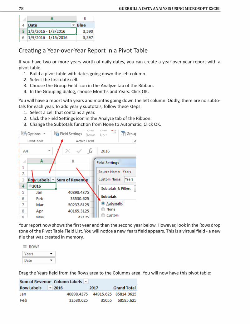
78 GUERRILLA DATA ANALYSIS USING MICROSOFT EXCEL
Creating a Year-over-Year Report in a Pivot Table
If you have two or more years worth of daily dates, you can create a year-over-year report with a pivot table.
1. Build a pivot table with dates going down the left column.2. Select the first date cell.3. Choose the Group Field icon in the Analyze tab of the Ribbon.4. In the Grouping dialog, choose Months and Years. Click OK.
You will have a report with years and months going down the left column. Oddly, there are no subto-tals for each year. To add yearly subtotals, follow these steps:
1. Select a cell that contains a year.2. Click the Field Settings icon in the Analyze tab of the Ribbon.3. Change the Subtotals function from None to Automatic. Click OK.
Your report now shows the first year and then the second year below. However, look in the Rows drop zone of the Pivot Table Field List. You will notice a new Years field appears. This is a virtual field - a new tile that was created in memory.
Drag the Years field from the Rows area to the Columns area. You will now have this pivot table:

USING PIVOT TABLES 79
Instead of the Grand Total, it would be better to show a % Change column. You are not allowed to create calculated fields in a pivot table with grouped dates, so you will have to build the calculation outside of the pivot table.
CAUTIONCalculations that point into pivot tables often encounter the GetPivotData bug.
To replace the Grand Total Column with a Percentage Change calculation, follow these steps:1. Make sure to select any cell inside of the pivot table.2. Select Design | Report Layout | Show in Tabular Form. This replaces headings such as Row
Labels and Column Labels with meaningful headings.3. Select Design | Grand Totals | On For Columns Only. This will keep the Grand Total Row and
remove the Grand Total Column. You might agree that the words "On For Columns Only" are one of the most awkward ways of saying "Delete the Grand Total Column".
4. Add a heading for % Change.5. In the first cell where the percentage should appear, type the formula =C5/B5-1. Do not use the
mouse or the arrow keys to enter this formula or Excel will change the formula to a GetPivotData function.
6. Format that cell as a percentage with 1 decimal place.7. Double click the fill handle to copy the formula down.
You should have results like this:
If every number in the % Change field is exactly identical, you used the mouse or the arrow keys when building the formula. Excel automatically replaced your correct formula with the hard-coded =GETPIVOTDATA formula shown below.
One common question is how to prevent GETPIVOTDATA from appearing. The first option is to build your external formulas by typing them and not using the mouse or arrow keys to point to cells inside the pivot table.
The permanent option:1. Select any cell inside the pivot table to bring the PivotTable Tools tabs back in the Ribbon.

80 GUERRILLA DATA ANALYSIS USING MICROSOFT EXCEL
2. On the Analyze tab, next to the Options button is a tiny dropdown. Open this dropdown.3. Unselect the choice for Generate GetPivotData.
What is the Point of GetPivotData?
Why would you ever use GetPivotData? It is great for taking pivot table data and re-using it in a non-pivot table report. The key to using the formula is to change the formula that Excel builds and replace the hard-coded text with cell addresses.
For example, say that you wanted to fill in this table using results from a pivot table. Select the first result cell. Type an equals sign. Using the mouse, click on the correct cell in the pivot table to return 2016, Q1, Red.
In the figure above, you can see that the formula generated by Excel is hard-coded to include "Red", 2016, and 1 for the Quarter. If you tried to copy this formula to other cells, it would still be pointing at Red, 2016, Q1.
You have to edit the formula to replace the hard-coded values with cell addresses.
You now have a formula that can be copied throughout your report. Note that while pivot table formatting is often ugly and wouldn't fly as a report for senior management, the shell report shown above can be formatted using any of Excel's formatting tools.
Using the Pivot Table to Get a Sum & Average at the Same Time
In the following Pivot Table, drag Ounces into the Values field of the field list twice. As you can see in the following figure, the default is Sum of Ounces. The second entry is Average of Ounces2. Click the dropdown arrow for this second entry and select Value Field Settings. In the Value Field Settings dialog, select Average and click OK.

USING PIVOT TABLES 81
The Pivot Table now tells you that for ultramarine blue powder, the July and August averages were about the same, but the total amount in August was almost half of the total in July. This suggests a lot fewer transactions, as opposed to the transactions just being smaller.
Using the Pivot Table to Get the Percentage of the Total
What if you want to see your data in percentages? A Pivot Table can do that for you.
In the Pivot Table from the preceding section, click the dropdown arrow for Average of Ounces2 in the field list. In the Value Field Settings dialog, highlight Sum in the Summarize Values By tab. In the Show Values As tab, open the Show Values As dropdown list and select % of Column Total, as shown in the next figure. Click OK.

82 GUERRILLA DATA ANALYSIS USING MICROSOFT EXCEL
As shown here, change the filter in B1 to (All):
Here’s what the Pivot Table tells you: ● Cell I14 shows that ultramarine blue accounted for 12.68% of the total ounces in July, August,
and September. ● In September, 1,638 ounces of electric blue was 23.34% of the month’s total.
Using the Pivot Table to Filter for the Top Five
Say that you want to work with only the colors with the top five overall ounces. With the cursor in cell A4, open the dropdown list and select Value Filters | Top 10, as shown in the next figure.
Change the default from 10 to 5, as shown in the next figure, and click OK.

USING PIVOT TABLES 83
Now you have just the top five, as shown here:
It gets even better! You can filter the columns for just gels. The list of colors changes because the Pivot Table is filtering for the colors with the top five ounces of gel.
Using the Pivot Table to Drill Down for Isolated Details
Now say that you want specific details about the 919 ounces of lime green powder, as shown here:

84 GUERRILLA DATA ANALYSIS USING MICROSOFT EXCEL
Double-click D10, and Excel creates a new page consisting of just lime green powder:
Making Many Copies of a Pivot Table
This trick is from Szilvia Juhasz, an amazing Excel trainer in Santa Monica. If you need Excel training, contact Szilivia @XSzil on Twitter.
1. Build any pivot table. In the example below, you can see the rank of Gels, Powder, and Oils.2. Say that you want to see this report for each color sold. Add the Color field to the Report Filter
area in the Pivot Table Field List.3. Go the the Analyze tab in the ribbon. Do not click the Options button. Instead, choose the
dropdown arrow to the right of the Options button. Choose Show Report Filter Pages.
4. Excel will provide a list of all the fields in the Filter area. In this case, there is only one field. Select Color and Click OK.
Excel will replicate the pivot table for each color in the original data set.

USING PIVOT TABLES 85
Deleting a Pivot TableIt’s not possible to delete a row or column in a Pivot Table. If you try to do it, you’ll get an error. But you can completely get rid of a Pivot Table, using three different methods:
● Option 1: Highlight all the columns of the Pivot Table and press Delete. ● Option 2: Highlight all the rows of the Pivot Table and press Delete. ● Option 3: Right-click the worksheet tab and choose Delete, as shown in the figure below.
CAUTIONWhen you delete an entire worksheet, you cannot reverse the action by using
Undo. Excel warns you of this when you try to delete a Pivot Table.
Overriding the Default Row Sequence in a Pivot TableAs the next figure shows, the default row labels are sorted in alphabetical order. You might want to override this order and sort the rows in another order, such as by the sum of ounces.
To change the sort order, click the dropdown arrow in cell A4 and select More Sort Options. In the Sort (Color) dialog, change the settings from their defaults to Descending and Sum of Ounces. Click OK, and you get the Pivot Table shown in the next figure.

86 GUERRILLA DATA ANALYSIS USING MICROSOFT EXCEL
Using Calculated Items & Calculated FieldsSometimes you need an additional dimension in your analysis and want to combine the source data in a way that isn't directly available. Pivot Tables give you calculated fields and calculated items to help. They’re handy, but they aren’t perfect, and I’ll make note of the limitations as we go through the examples.
Working with Calculated Items
A calculated item is an item added to a field. Specifically, it’s an item that doesn’t exist in the source data.
In the data you’ve been working with, it’s clear that blues and reds see far more activity than other colors, so now you’ll create calculated items for the following:
● Blues ● Reds ● Other colors
CAUTIONYou cannot use grouping and calculated items in the same Pivot Table.If you have already grouped data and later want to add a calculated item, you
need to ungroup the data by right-clicking in the field that has been grouped and selecting Ungroup. If you have a calculated item and want to group some-thing, you simply can’t do it.
With the cursor in one of the row labels, go to the ribbon and select Analyze |Calculations | Fields, Items, & Sets | Calculated Item:
In the Insert Calculated Item dialog that appears, make the changes shown in the following figures, clicking OK when you’re done with each one.

USING PIVOT TABLES 87
The following figure shows the sum of ounces for the colors, and the calculated fields that you just created for All Blues, All Reds and Other Colors.
CAUTIONNotice that the calculated items show
up as additions to the original data. Therefore, the grand total appears twice as large with the calculated items as it is in reality. Be careful! Make sure to use your filters so that you don’t mix the original color items and the summarized calculated items.

88 GUERRILLA DATA ANALYSIS USING MICROSOFT EXCEL
Notice the formula that appears in the calculated field. In cell B6 you see:=SUM(Espresso,’Lemon Yellow’,Lilac,’Lime Green’,Silver)
Also notice that you need to use single quotes for terms that are more than one word.
Working with Calculated FieldsSay you know that roughly 3% of inventory is lost to spills, inaccurate weighing, samples taken for developing new products, etc. Therefore, to really keep track of inventory levels, you should add an additional 3% in your analysis. Here’s an example:
(4,778 ounces of electric blue) x 103% = 4,921.34 ounces
To have Excel handle this calculation for you, you can create a calculated field called Sold+Lost. To do so, with your cursor in one of the column headers, select Analyze | Fields, Items, & Sets | Calculated Field. In the Insert Calculated Field dialog, shown next, enter the formula =Ounces*1.03.
In the next figure, you see that the new Sold+Lost field shows up as an available entry in the field list.
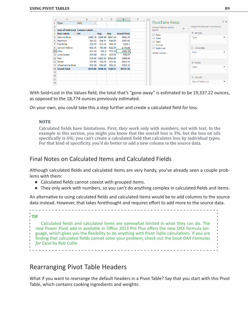
USING PIVOT TABLES 89
With Sold+Lost in the Values field, the total that’s “gone away” is estimated to be 19,337.22 ounces, as opposed to the 18,774 ounces previously estimated.
On your own, you could take this a step further and create a calculated field for loss.
NOTECalculated fields have limitations. First, they work only with numbers, not with text. In the example in this section, you might you know that the overall loss is 3%, but the loss on oils specifically is 6%; you can’t create a calculated field that calculates loss by individual types. For that kind of specificity, you’d do better to add a new column in the source data.
Final Notes on Calculated Items and Calculated Fields
Although calculated fields and calculated items are very handy, you’ve already seen a couple prob-lems with them:
● Calculated fields cannot coexist with grouped items. ● They only work with numbers, so you can’t do anything complex in calculated fields and items.
An alternative to using calculated fields and calculated items would be to add columns to the source data instead. However, that takes forethought and requires effort to add more to the source data.
TIPCalculated fields and calculated items are somewhat limited in what they can do. The
new Power Pivot add-in available in Office 2013 Pro Plus offers the new DAX formula lan-guage, which gives you the flexibility to do anything with Pivot Table calculations. If you are finding that calculated fields cannot solve your problem, check out the book DAX Formulas for Excel by Rob Collie
Rearranging Pivot Table HeadersWhat if you want to rearrange the default headers in a Pivot Table? Say that you start with this Pivot Table, which contains cooking ingredients and weights:

90 GUERRILLA DATA ANALYSIS USING MICROSOFT EXCEL
You want to move Brown Sugar to the right, next to White Sugar, where it would make more sense. Highlight Brown Sugar and drag it to the place you want it. As shown in the next figures, the Pivot Table moves the data that corresponds with that heading.
Pivot Table Q&A
What if I don’t want a grand total column or a grand total row?
In some situations, totals give you nonsense, or you simply don’t want totals. The following figure shows data about cyclists. They aren’t on a team and aren’t competing. You just want totals for each individual. Therefore, having a monthly total means nothing in this case.

USING PIVOT TABLES 91
To get rid of the grand totals, you select Pivot Table Tools | Design | Grand Totals | On for Rows Only:
The next figure shows that you can now easily see that Vy has cycled 182 miles, and you aren’t distracted with monthly summaries.
When I change a number in the source data, does it automatically update in the Pivot Table?
Not necessarily. There are three distinct situations: ● If you change a number within the range of the original data—such as incorrectly input an 8
cycling miles for a user on a day when he actually did 18 miles—and want to fix it, you have to do a little work to have the Pivot Table reflect the change: 1. Correct the number in the source data.2. Go back to the Pivot Table and select any cell in it. 3. Right-click and select Refresh.
● If you add new data that extends the original range, after you add the new data to the source data, you need to follow these steps:1. Click in any cell of the Pivot Table and select Pivot Table Tools | Analyze | Change Data
Source | Change Data Source. The Change Pivot Table Data Source window appears, with the original data range showing.
2. Change the range to include the new data. For example, in the following figure I’ve added 16 rows of August data.

92 GUERRILLA DATA ANALYSIS USING MICROSOFT EXCEL
3. When you return to the Pivot Table, it shows the new data for August.
● If the source data is in an Excel table, you can just right-click and refresh. The new Pivot Table will reflect the revised data, added or deleted rows, and added or deleted columns.
Can I make a Pivot Table of multiple Pivot Tables?
The person who asked this really wants to create a data model. That’s discussed later in this book. See "Understanding Data Models and Relationships" on page 121.
Pivot Table ConclusionsPivot Tables and VLOOKUP are Excel features that fantastically increase efficiency, ease headaches, and improve the accuracy of results. Explore Pivot Tables! This section has only scratched the surface of this tool that can do some amazing things for you.
Where users struggle with Pivot Tables is really when their data isn't ready to go into the Pivot Table. Therefore, it's important to work with contiguous data sets (page 25) and use good spreadsheet layouts (page 168).
With your data set up properly, Pivot Tables can help you easily take your analysis to the extreme.
Using Array FormulasImagine writing a single formula that could eliminate the need for helper columns and the dozens or hundreds or thousands of formulas that would be in each helper column. Imagine a formula that can return more than one result! Such a feature does exist in Excel. They’re called array formulas aka CSE formulas because Ctrl+Shift+Enter are the required keystrokes for completing an array/CSE formula.

178 GUERRILLA DATA ANALYSIS USING MICROSOFT EXCEL

INDEX 179
IndexSymbols24 Hours 150#N/A error
VLOOKUP 65#NAME? 119#REF! error 4
AAccounting underline 25Adding data
to formula 15Advanced Filter 40Alt+Enter 26Application key 4ARABIC 153Array constant 98Array formulas 92Arrow keys 176
BBAHTTEXT 153Barresse, Zack 107Basics 2Berry, Troy viiiBlank cells
Replace with 0 50Blank columns 25Blog post 140Boolean logic 144Bouchez, Helena viii
CCase study 168CEILING 157Cell references
Relative & absolute 9Center Across Selection 27Chaney, Keidra viiiCharting 119
3D 127Data 126Data Labels 125Histogram 96Logarithmic scale 119Orders of magnitude 119
CHOOSE 161Collie, Rob 89Combo Charts 121Comparing lists 61Concatenate names 3Conditional Formatting 16
Find duplicates 19Manage rules 18
Consolidate 47Annoyances 50
Functions 50Multiple data sets 48
Contiguous data 25CONVERT 158COUNTA 32, 155COUNTIF 23COUNTIFS 58, 60Counting
using Criteria 58Crickets ixCrossfooting 165CSE formulas 92Curly braces
around formula 93Current date 148Custom lists 29
DData integrity 112Data Models 137DataScopic.net viiData Validation 113
Dates 114Error Alert 116Formula-based 116List 113Numbers 114Times 116
Datechange to numbers xCurrent 148Functions 148Rollups 75
DATE 148DAX Formulas for Excel 89DAY 148DAYS 148Deadlines
Conditional formatting 17Download files 1Drill Down 83Dropdown Lists 104, 113Duplicates
Filtering 43Finding 19
Dynamic spreadsheets 15
EEmbedding Excel 140End Key 173End of Month 163EOMONTH 148, 163Error Alert 116Error handling 118Evaluate Formula 166Excel Web App 140
Differences 143
F

180 GUERRILLA DATA ANALYSIS USING MICROSOFT EXCEL
F4for Redo 176
Few, Stephen 127Field Buttons 132Filtering 32
Advanced 40And/Or criteria 42by Selection 37Copy fields 42Copy to location 42Custom 38Dates 40Dropdown arrows 33in Place 41Top 5 36Unique 43with Formula 44
FIND 145Fit to Page 143FLOOR 157FORECAST 155Formatting
Conditional 16Formula entry 176Formula Evaluator 166Formulas 2
to Values 3FREQUENCY 95Functions 154
GGETPIVOTDATA
Bug 79Use for 80
Go To Special 50, 52Graphing 119
3D 127Data Labels 125
GridlinesHiding 152
HHeadings
Single row 26Helper columns 7Hide columns 8Histogram 95
IIcon sets 20
Icon only 21IF 22, 118IFERROR 119IFNA 119INDEX & MATCH 66INDIRECT 107
with VLOOKUP 109
J
Join text 3Jones, Kevin 107Juhasz, Szilvia 84
KKeyboard Shortcuts 173
LLARGE 158Layout 171LEFT 145LEN 145Linking 11, 12
Workbooks 14Loan payment 154Logarithmic scale 119Lookup. See also VLOOKUP Function
Two-way 67LOWER 145
MMail merge xManage rules 18MATCH 62, 67Matching lists 61MAX 158Merged cells 27
Center Across Selection 27MID 145MIN 158Minutes 151ModelOff 176MONTH 148MrExcel.com viiiMultiply
all cells in range 6MVP Award viii
NNest functions 9NETWORKDAYS 148NOW 148Number formats 149
OOFFSET 110Olympics, Excel 176OneDrive 141Overtime 7
PPaste as Values 4Paste Special
Multiply 6Transpose 5Values 4
Payment 154Peltier, Jon 127

INDEX 181
Pivot Charts 127Chart type 132Field Buttons 132Slicers 132
Pivot Tables 68Better column headings 79Calculated Fields 88Calculated Items 86Creating 71Deleting 85Drill Down 83Field Settings 74Filtering 70, 75for Counting 69for Summing 69Grand total 90Group by week 77Grouping dates 75Multiple sources 138% of Total 81Rearranging 89Refreshing 91Show Values As 81Tabular layout 79Top Five 82Use zero for blanks 74Wizard 72Year over year 78
PMT 154Podcast viiiPROPER 145
RRAND 159RANDBETWEEN 159Random assignments 160RANK 155Redo 176Relationships 137Relative cell references 9Remove Duplicates 48Replace current subtotals 54RIGHT 145ROMAN 153Rounding 157
SSecond City viii, ixShow formulas 165Silver, Nate xSlicers 132, 133
with Tables 136SMALL 158Sorting 24
Days of the week 28Helper column 31Icons 28Quick sort 28Two criteria 30
Spreadsheet design
Fundamentals 25Star icons 20Subtotals 51
Multiple levels 54Prevent pivoting 58
SUMvs. adding cells 153
SUMIFS 58, 60Summing
using Criteria 58SUMPRODUCT 163
TTables 99
Adding columns 101Adding rows 101Mixing formulas 106Protection 107Total Row 103VLOOKUP 104
Templates 107TEXT 149Text functions 145Time
Adding 150Formats 151
Tips 143TODAY 148Top 5 36Top Five
with Pivot Table 82Torture chamber 1Transpose 5Treacy, Mynda 127TRIM 145Tri-State checkbox 27Troubleshooting
Edit mode 167Evaluate formula 166
Tufte, Edward 127Turn sideways 5Two-way lookup 67
UUndo 4Unhide column A 152UPPER 145USS Joseph Hewes viiUSS Sturgeon vii
VVisible Cells Only 52Visual Filters 133VLOOKUP 64
Approximate? 65Leading spaces 65Left of key? 66Range lookup 66to other worksheet 13
True 65vs. CHOOSE 161with Tables 104
WWEEKDAY 148Wrap text 26
YYEAR 148Year over year 78YouTube viii

More Titles from Holy Macro! Books