Guaranteeing the Topology of an Implicit Surface Polygonization forInteractive Modeling

Barton T. Stander1 John C. Hart2

School of EECSWashington State University

Abstract

Morse theory shows how the topology of an implicit surface is af-fected by its function’s critical points, whereas catastrophe theoryshows how these critical points behave as the function’s parameterschange. Interval analysis finds the critical points, and they can alsobe tracked efficiently during parameter changes. Changes in thefunction value at these critical points cause changes in the topology.Techniques for modifying the polygonization to accommodate suchchanges in topology are given. These techniques are robust enoughto guarantee the topology of an implicit surface polygonization, andare efficient enough to maintain this guarantee during interactivemodeling. The impact of this work is a topologically-guaranteedpolygonization technique, and the ability to directly and accuratelymanipulate polygonized implicit surfaces in real time.

Descriptors: I.3.5 Computational Geometry and Object Modeling— Modeling packages.General Terms: Algorithms.Keywords: catastrophe theory, critical points, implicit surfaces,Morse theory, polygonization, topology, interval analysis, interac-tive modeling, particle systems.

1 Introduction

Shapes are represented implicitly by a function that classifies pointsin space as inside the shape, outside the shape or on the shape’ssurface, called the implicit surface. This representation providescomputer graphics with geometric models that can be easily andsmoothly joined together, but the incorporation of the implicit rep-resentation into graphics systems can be problematic. Polygoniza-tion of implicit surfaces allows graphics systems to reap the power-ful modeling benefits of the implicit representation while retainingthe rendering speed and flexibility of polygonal meshes.

The topology (specifically thehomotopy type) of an implicitsurface refers to the connectedness of the shape, including the num-ber of disjoint components and the number of holes in each com-ponent (genus). This should not be confused with other instances

1Current address: Strata, 1562 El Vista Circle, Saint George, UT 84765,barts@strata3d.com

2Address: School of EECS, WSU, Pullman, WA 99164-2752,hart@eecs.wsu.edu

of topology in computer graphics, such as the connection patternsof a mesh of polygons or parametric patches. Thus, for a polygo-nization to accurately represent the topology of an implicit surfacethe number of components and the genus of each component of thepolygonization need to agree with that of the implicit surface.

Implicit surfaces are commonly polygonized to a given degreeof geometric accuracy. This accuracy is in some cases adaptivelyrelated to the local curvature of the implicit surface, reducing thenumber of polygons without affecting the appearance of the sur-face. This work instead focuses on a polygonization that accu-rately discerns the topology of an implicit surface. Topologically-accurate polygonization can reduce the number of polygons with-out affecting the structure of the surface.

Guaranteeing the topology of a polygonization does not neces-sarily yield an accurate polygonization. A coffee cup is topologi-cally equivalent to a torus, but the torus provides a poor represen-tation for the geometry of a coffee cup. The topological guaranteebecomes useful when coupled with a geometrically accurate poly-gonization scheme.

Guaranteeing the topology of an implicit surface polygoniza-tion solves several open problems in computer graphics.

Polygonization topology is coordinate dependent.Polygoniza-tion schemes often discern topology from point samples. Differentpolygonizations of the same implicit surface may differ in topol-ogy, and the same polygonization algorithm may return differenttopological structures depending on the coordinate system of theimplicit surface, as demonstrated in Figure 1. For example, the im-plicit surface might appear connected when polygonized in its mod-eling coordinate system but could then appear disconnected whenpolygonized in a scene’s coordinate system.

(c)(a) (b) (d)

Figure 1: The topology of a connected implicit surface is correctlypolygonized (a), but a translated instance is not (b). Two disjointcomponents are polygonized as a single component (c), but a trans-lated instance is polygonized properly (d).

Interloping components.Some configurations of implicit surfacescan yield unexpected disjoint components. Such isolated compo-nents of the implicit surface occur because of an accumulation ofneighboring potentials but do not themselves surround any “skele-

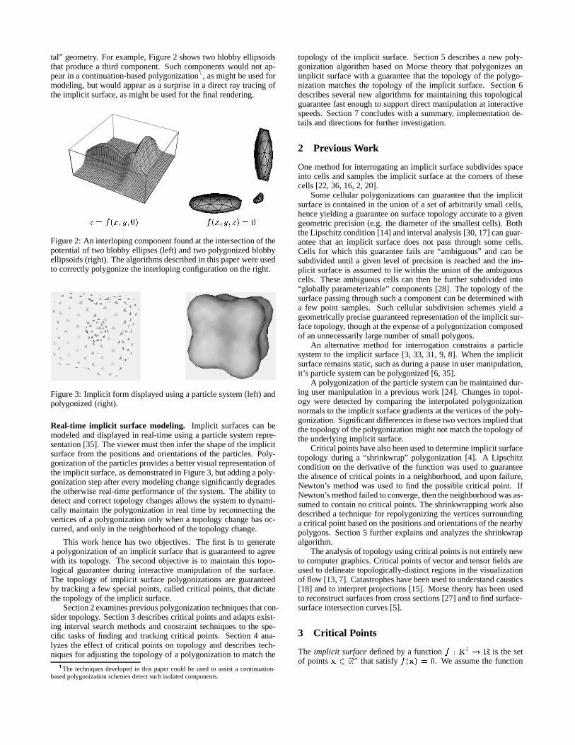
tal” geometry. For example, Figure 2 shows two blobby ellipsoidsthat produce a third component. Such components would not ap-pear in a continuation-based polygonization1 , as might be used formodeling, but would appear as a surprise in a direct ray tracing ofthe implicit surface, as might be used for the final rendering.

z = f(x; y; 0) f(x; y; z) = 0

Figure 2: An interloping component found at the intersection of thepotential of two blobby ellipses (left) and two polygonized blobbyellipsoids (right). The algorithms described in this paper were usedto correctly polygonize the interloping configuration on the right.

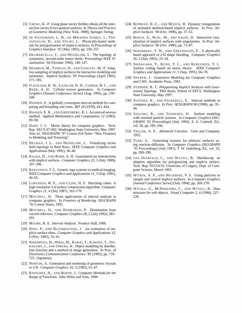
Figure 3: Implicit form displayed using a particle system (left) andpolygonized (right).

Real-time implicit surface modeling. Implicit surfaces can bemodeled and displayed in real-time using a particle system repre-sentation [35]. The viewer must then infer the shape of the implicitsurface from the positions and orientations of the particles. Poly-gonization of the particles provides a better visual representation ofthe implicit surface, as demonstrated in Figure 3, but adding a poly-gonization step after every modeling change significantly degradesthe otherwise real-time performance of the system. The ability todetect and correct topology changes allows the system to dynami-cally maintain the polygonization in real time by reconnecting thevertices of a polygonization only when a topology change has oc-curred, and only in the neighborhood of the topology change.

This work hence has two objectives. The first is to generatea polygonization of an implicit surface that is guaranteed to agreewith its topology. The second objective is to maintain this topo-logical guarantee during interactive manipulation of the surface.The topology of implicit surface polygonizations are guaranteedby tracking a few special points, called critical points, that dictatethe topology of the implicit surface.

Section 2 examines previous polygonization techniques that con-sider topology. Section 3 describes critical points and adapts exist-ing interval search methods and constraint techniques to the spe-cific tasks of finding and tracking critical points. Section 4 ana-lyzes the effect of critical points on topology and describes tech-niques for adjusting the topology of a polygonization to match the

1The techniques developed in this paper could be used to assist a continuation-based polygonization schemes detect such isolated components.

topology of the implicit surface. Section 5 describes a new poly-gonization algorithm based on Morse theory that polygonizes animplicit surface with a guarantee that the topology of the polygo-nization matches the topology of the implicit surface. Section 6describes several new algorithms for maintaining this topologicalguarantee fast enough to support direct manipulation at interactivespeeds. Section 7 concludes with a summary, implementation de-tails and directions for further investigation.

2 Previous Work

One method for interrogating an implicit surface subdivides spaceinto cells and samples the implicit surface at the corners of thesecells [22, 36, 16, 2, 20].

Some cellular polygonizations can guarantee that the implicitsurface is contained in the union of a set of arbitrarily small cells,hence yielding a guarantee on surface topology accurate to a givengeometric precision (e.g. the diameter of the smallest cells). Boththe Lipschitz condition [14] and interval analysis [30, 17] can guar-antee that an implicit surface does not pass through some cells.Cells for which this guarantee fails are “ambiguous” and can besubdivided until a given level of precision is reached and the im-plicit surface is assumed to lie within the union of the ambiguouscells. These ambiguous cells can then be further subdivided into“globally parameterizable” components [28]. The topology of thesurface passing through such a component can be determined witha few point samples. Such cellular subdivision schemes yield ageometrically precise guaranteed representation of the implicit sur-face topology, though at the expense of a polygonization composedof an unnecessarily large number of small polygons.

An alternative method for interrogation constrains a particlesystem to the implicit surface [3, 33, 31, 9, 8]. When the implicitsurface remains static, such as during a pause in user manipulation,it’s particle system can be polygonized [6, 35].

A polygonization of the particle system can be maintained dur-ing user manipulation in a previous work [24]. Changes in topol-ogy were detected by comparing the interpolated polygonizationnormals to the implicit surface gradients at the vertices of the poly-gonization. Significant differences in these two vectors implied thatthe topology of the polygonization might not match the topology ofthe underlying implicit surface.

Critical points have also been used to determine implicit surfacetopology during a “shrinkwrap” polygonization [4]. A Lipschitzcondition on the derivative of the function was used to guaranteethe absence of critical points in a neighborhood, and upon failure,Newton’s method was used to find the possible critical point. IfNewton’s method failed to converge, then the neighborhood was as-sumed to contain no critical points. The shrinkwrapping work alsodescribed a technique for repolygonizing the vertices surroundinga critical point based on the positions and orientations of the nearbypolygons. Section 5 further explains and analyzes the shrinkwrapalgorithm.

The analysis of topology using critical points is not entirely newto computer graphics. Critical points of vector and tensor fields areused to delineate topologically-distinct regions in the visualizationof flow [13, 7]. Catastrophes have been used to understand caustics[18] and to interpret projections [15]. Morse theory has been usedto reconstruct surfaces from cross sections [27] and to find surface-surface intersection curves [5].

3 Critical Points

The implicit surfacedefined by a functionf : R3 ! R is the set

of pointsx 2 R3 that satisfyf(x) = 0. We assume the function

returns positive values inside the object, so thesolid modeled bythe implicit surface is the set of pointsfxjf(x) � 0g:

This work requires the functionf to beC2 continuous, withcontinuous first and second derivatives, and its implicit surface mustbe a manifold with a well defined, continuously varying surfacenormal. These restrictions include exponential-based “blobby” mod-els [1], but exclude some of the more efficientC1 piecewise poly-nomial approximations [21, 36].

The implicit surface is extended into a family of surfaces de-fined byf(x;q) continuously parameterized by the vectorq con-sisting of various model parameters (e.g. the locations of blobbyelements). For some values ofq; the implicit surface defined byf(x;q) = 0 may contain a cusp, kink or crease, specifically whenthe implicit surface changes topology. We consider the implicit sur-faces in this family before and after but not during such topologychanges. An alternative technique exists for interactively manipu-lating implicit surfaces with cusps, kinks and creases [25].

Thecritical pointsof a functionf occur where its gradient

rf(x) = (fx(x); fy(x); fz(x)) (1)

vanishes. (The notationfx = @f=@x:) A critical value is the valueof the functionf at a critical point.

The HessianV (called thestability matrix in catastrophe the-ory) is defined as the Jacobian of the gradient

V (x) = J(rf(x)) =

"fxx(x) fxy(x) fxz(x)fyx(x) fyy(x) fyz(x)fzx(x) fzy(x) fzz(x)

#: (2)

Sincefxy = fyx; etc., the stability matrix is symmetric.A critical point x is classified based on the signs of the three

eigenvaluesl1 � l2 � l3 of V (x) [32]. If all three eigenvaluesare non-zero, then the critical point is callednon-degenerateand iseither a maximum, minimum or some kind of saddle point. In threedimensions, saddle points come in two varieties. Table 1 indicatesthis classification.

l1 l2 l3 Critical Point- - - Maximum Point- - + 2-Saddle- + + 1-Saddle+ + + Minimum Point

Table 1: Classification of critical points based on the sign of theeigenvalues of the stability matrix.

The critical points are continuously dependent on the parame-ter vectorq: As the parameter vectorq changes, the critical pointsmove in space. They can also appear spontaneously in pairs, orcollide in pairs, annihilating each other. If any of the three eigen-values of the stability matrix of a critical point equal zero thenxis called adegenerate critical point.The creation and destructionof critical points occur at degenerate critical points Critical pointcreation/destruction is demonstrated in Figure 4.

Isolated degenerate critical points are unstable. In the rare eventthat an isolated degenerate critical point does appear, it can be re-moved by a small perturbation of the implicit surface parameterswithout affecting the implicit surface topology.

Some functions can yields non-isolated degenerate critical points(critical sets). For example, the cylinder defined byf(x; y; z) =

x2+y2�1 has a critical line along thez-axis. A small perturbationof the cylinder into an ellipsoidf(x; y; z) = x2 + y2 + �z2 � 1

collapses the degenerate critical line into a single non-degeneratecritical point at the origin. We assume the family of implicit sur-faces is parameterized such that degenerate sets can be removed bysuch perturbation.

★ ★

★

★

★★

(a) (b) (c)

Figure 4: Creation of critical points in 1-D:y = f(x; 0; 0): (a) Twosummed Gaussian bumps, one large and one small, sufficientlyclose such that there is only a single maximum point in the do-main shown. (b) Moving the smaller bump away from the largercreates a degenerate critical point. (c) Moving the smaller bumpfarther results in the creation of a pair of new critical points: amaximum point and a minimum point. Performing these steps inreverse demonstrates critical point annihilation.

3.1 Finding All Critical Points

Interval analysis searches can be guaranteed to find all points satis-fying a given criterion in a given bounded domain to a desired de-gree of accuracy [19, 23]. Such a search can find all of the criticalpoints of a given function to determine the topology of its implicitsurface.

The interval search for critical points starts with an initial boxbounding the space of interest. The simple interval search for criti-cal points shown in Figure 5 eliminates large portions of space thatcannot contain a critical point.

Given a box (a vector of intervals)X = [x0; x1] � [y0; y1] �[z0; z1] the algorithm checks whether the intervals returned by allof the partial derivatives contain zero. If not, thenX contains nocritical points. If so, then the algorithm subdividesX and tests eachcomponent individually. Note thatFx(X) is an interval arithmeticimplementation of@f=@x; and likewise forFy; Fz:

Procedure SimpleSearch(X)If diam(X) < � then indicate critical point inX:If 0 2 Fx(X) and0 2 Fy(X) and0 2 Fz(X) then

SubdivideX and continue the search recursively.

Figure 5: Simple interval divide and conquer search algorithm.

In these algorithms, subdivision means dividing into halves withrespect to its widest axis, although any number of subdivision tech-niques could be used. The diameter of a boxdiam(X) is measuredusing the chessboard metric, and is simply the width of the widestinterval-element in the vectorX:

Simple subdivision performs remarkably well, discarding largeportions of space known not to contain critical points. This tech-nique will eventually finds all critical points to any degree of accu-racy within a given bounding box, but with only linear convergence.

When the box diameter reaches a given size, the quadratically-convergent interval Newton’s method shown in Figure 6 refinesand/or subdivides the box down to the desired numerical precision[28, 11].

Given two pointsx;y there exist pointsz between2 x andysuch that

rf(x) + V (z)(y� x) = rf(y); (3)

where the stability matrixV is the Jacobian ofrf: Letm(X) re-turn the midpoint of boxX. The algorithm seeksy 2 X such thatrf(y) = 0: Since bothx;y 2 X; thez satisfying (3) must be inX as well. Thus, solving

rf(m(X)) + V (X)(Y �m(X)) = 0: (4)

yieldsY; a box containing all of the critical points inX: Note that

Procedure NewtonSearch(X)Repeat.

SolveV (X)(Y�m(X)) = �rf(m(X)) for Y:If Y � X then subdivideX and search recursively.If Y � X then there is a unique c.p. inY (andX).If Y \X = ; then there is no c.p inX: Return.Otherwise letX = X \Y:

Until diam(X) < �:Indicate critical point atm(X):

Figure 6: Interval Newton’s method search for critical points.

V (X) returns a matrix of intervals.An interval version of Gauss-Seidel is recommended for solv-

ing (4), but this can lead to two problems. First, the diagonal el-ements ofV (X) might contain zero, requiring the interval arith-metic division operation to correctly perform a division by an inter-val containing zero. Division by intervals containing zero producetwo intervals, leading to additional algorithm recursion [28, 10].Solving the rows whose diagonal elements do not contain zero firstreduces the occurrence of semi-infinite intervals [11].

Solving

V�1

c V (X)(Y � x) = �V�1

c rf(m(X)): (5)

whereVc = m(V (X)) instead of (4) yields a much tighter boundand hastens the NewtonSearch performance [11]. Note that theexpressionm(V (X)) returns a scalar matrix consisting of the mid-points of the intervals ofV (X):

When a critical point lies on an edge of the box, NewtonSearch’sconvergence is less quadratic. ExtendingX outward by a smallpercentage each iteration avoids this problem. Time may also beincorporated into the search by crossingX with the time interval[t0; t1]:

3.2 Tracking Critical Points

Altering an implicit surface’s parameters changes the positions ofsome or all of the critical points.

The same techniques that constrain particles to adhere to theimplicit surface [35], can also cause particles to adhere to any se-lected critical point.

Letx = x(t) be a particle constrained to follow one of the criti-cal points of the functionf: Its partial derivativesfx(x); fy(x); andfx(x) are all constrained to zero. To ensure that they remain zero,

their time derivatives_fx(x) = d2f

dxdt(x); _fy(x) and _fz(x)must also

be set to zero. Given the parameter vectorq and its velocity_q; onecan solve these equations to determine the critical point velocity_x.This velocity is then passed to a differential equation solver (suchas fourth-order Runge-Kutta) to approximate the new location ofthe critical point. Newton’s method refines the approximation.

4 Detecting and Correcting Topology Changes

The identification of critical points simplifies topologically-guar-anteed direct manipulation of implicit surfaces through a polyg-onal representation. The key to solving the topology problem isthat a change in the topology of a surface is always accompaniedby a change in the sign of a critical value [12]. Monitoring thecritical points greatly simplifies the burden of detecting topologi-cal changes, and divides the problem into classifying topologicalchanges, identifying polygons to remove and reconnecting the ver-ticed of the removed polygons.

2The notion of “between” for points in space means thatz is in a box with cornersat x andy.

4.1 Classifying Topological Changes

Table 2 enumerates all of the possible critical-point/sign combina-tions and their corresponding implications on the implicit surfacetopology. When an implicit surface topology change is detected,the polygonization must be altered to properly represent the newtopology.

Critical Point Sign Changes To ActionMaximum - DestroyMaximum + Create2-Saddle - Cut2-Saddle + Attach1-Saddle - Pierce1-Saddle + SpackleMinimum - BubbleMinimum + Burst

Table 2: The affect of critical point sign on topology.

4.2 Identifying Polygons to Remove

Changes in maximum and minimum critical values cause entiresimply-connected components of polygonization to be removed orcreated. Changes in saddle points require the determination of spe-cific polygons to be removed such that their vertices may be prop-erly reconnected. These polygons intersect a separatrix extendingfrom the saddle point.

The separatrix may be efficiently approximated by a line for 2-saddles, or a plane for 1-saddles. These lines and planes describedby the eigenvectors of the stability matrix of a critical point approx-imate the separatrix.

When separatrixes are linearly approximated by lines and planes,certain errors might occur. For example, a 2-saddle may connecttwo components, but the line approximating its separatrix mightnot intersect either component. One must then assume that the pa-rameter vectorq is sufficiently close to the parameter vector at thetopology changeq� that the linear approximation correctly inter-sect the proper polygonized implicit surface components.

The separatrix extending from a 2-saddle can be treated as aninitial value problem, using the positive eigenvectorv3(x) of thestability matrix to define the ordinary differential equation

_x = v3(x) (6)

and using numerical integration to trace out the path of the separa-trix. The midpoint method provided sufficient numerical accuracyfor this task in our experiments.

The case where a separatrix intersects a polygonization vertexcan be removed with a topology-preserving perturbation.

4.3 Reconnection

The following procedures describe which polygons must be re-moved, and how their vertices are reconnected to update the topol-ogy of the polygonization.

Destroy. When the value at a maximum goes negative, an isolatedcomponent in the implicit surface disappears. A ray cast from themaximum point in any direction will first intersect a polygon inthis simply-connected component. All polygons connected to thispolygon are then removed. Figure 7 pseudocodes this algorithm.

Create. When the value at a maximum goes positive, a new, simply-connected component in the implicit surface appears. A sufficientlysmall tetrahedron may be placed around the maximum point, lettingits vertices adhere to the implicit surface component and adding

Procedure Destroy/BurstCast a ray from maximum point in any direction.Let p be the first polygon the ray intersects.Pushp onto stack.While stack not empty.

Let p be the result of popping the stack.For all polygonsq sharing an edge withp:

Pushq onto stack.Removep from polygonization.

Figure 7: The repolygonization algorithm forDestroyandBurst.

new polygons when necessary. Alternatively, a ray may be castfrom the maximum point and intersected with the implicit surface.The first intersection denotes the location where any standard con-tinuation polygonization technique may be applied. Figure 8 pseu-docodes this algorithm.

Procedure Create/BubbleCast a ray from maximum point in any direction.Let x 2 f�1(0) be the first ray intersection.Polygonize the component containingx:

Figure 8: The repolygonization algorithm forCreateandBubble.

Cut. When the value at a 2-saddle goes negative, part of the im-plicit surface disconnects. The separatrix surface extending fromthe 2-saddle is found by integrating the two negative eigenvalues ofthe stability matrix will intersect the polygons in a ring surround-ing the 2-saddle. In practical cases, this separatrix is sufficientlyapproximated by a plane passing through the 2-saddle perpendic-ular to its positive eigenvector. The ring of polygons intersectingthe separatrix surface are removed, yielding two disjoint rings ofpolygonization vertices. These rings are “sewn up” individually viatriangulation. Figure 9 pseudocodes this algorithm, and Figure 10illustrates the polygon configuration.

Procedure Cut/SpackleLet P be a plane containing the critical pointx perpen-

dicular to the uniquely-signed eigenvector ofV (x):Cast a ray fromx in any direction withinP:Let p0 be the first polygon intersected by the ray.Initialize i = 0 and repeat.

Let pi+1 be a polygon intersectingP; sharing an edgewith pi; and not equal to anypj for j � i:

If no suchpi+1 exists, break.Incrementi:

Let v0 be any vertex ofp0:Call Procedure Ring.Triangulatevi:Let v0 be any vertex ofp0 not currently triangulated.Call Procedure Ring.Triangulatevi:

Procedure RingInitialize i = 0 and repeat.

Let e be an edge connecting vertexvi to vi+1separating apk polygon from a non-pk polygon, andvertexvi+1 not equal to anyvj for j � i:

If no suchvi+1 exists, break.Incrementi:

Figure 9: The repolygonization algorithm forCutandSpackle.

+/−

−/+−/+

Figure 10: Polygons, eigenvalues and eigenvectors forCut andSpackle.

Attach. When the value at a 2-saddle goes positive, two com-ponents of the implicit surface connect. The separatrix curve ex-tends from the 2-saddle in the direction of its positive eigenvalueto a maximum point inside each component. The first polygon ineach direction the separatrix intersects is removed. This leaves twodisjoint rings of vertices that need to be connected. Proper corre-spondence algorithms between the two polygons can be found (e.g.[26]), but such techniques are not necessary if the polygonizationis restricted to triangles. Figure 11 pseudocodes this algorithm.

Procedure Attach/PierceExtend separatrix curves from the critical point.Let polygonsp0 andp1 first intersect each separatrix.Connect the vertices ofp0 with the vertices ofp1:Removep0 andp1:

Figure 11: The repolygonization algorithm forAttachandPierce.

Pierce. When the value at a 1-saddle goes negative, a hole ispierced in the implicit surface. Similar to theattachcase (a holein the implicit surface off is a connection in the implicit surfaceof �f ), the two polygons that intersect the separatrix curve pass-ing through the 1-saddle in the direction of the eigenvector corre-sponding to the one negative eigenvalue of the stability matrix areidentified. These two polygons are removed and now form the endsof the hole. Corresponding and connecting the resulting two ringsof vertices form the walls of the hole. The algorithm in Figure 11also repolygonizes thepiercecase.

Spackle. When the value at a 1-saddle goes positive, a hole inthe implicit surface is filled. Similar to thecut case, the separatrixsurface is constructed at the 1-saddle perpendicular to the eigen-vector corresponding to the one negative eigenvalue of the stabilitymatrix. The local polygons this surface pierces are removed, andthe two resulting polygonal holes are “sewn up” by triangulation.The algorithm in Figure 9 also repolygonizes thespacklecase andFigure 10 illustrates the polygon configuration.

Bubble. When the value at a minimum goes negative, a pocket of

air forms inside the implicit solid. An air pocket in the implicitsurface off is a new component in the implicit surface of�f:This pocket of air may therefore be treated as a simply-connectedimplicit surface component, and polygonized using any of the ex-isting techniques. The algorithm in Figure 8 also repolygonizes thebubblecase.

Burst. When the value at a minimum goes positive, an air bubblewithin the implicit solid has burst. As in the Destroy case, a rayis cast from the minimum in any direction. The first polygon thisray intersects, as well as any other polygons with a connection toit, are then removed. The algorithm in Figure 7 also repolygonizestheburstcase.

5 Polygonization

Morse theory provides the background for a topologically-guar-anteed polygonization algorithm. Given a function f(x) implicitlydefining the surfacef�1(0); we consider the family of surfacesf�1(a) for non-negativea: Let a0 be a value of sufficient magni-tude such that the surfacef�1(a0) = ;: As a0 decreases, it willpass critical values for maximum points, 2-saddles, 1-saddles andminimum points. As each critical value is encountered, the topol-ogy of the polygonization around its critical point is corrected. This“inflation” algorithm is pseudocoded in Figure 12.

Procedure InflateXc = SearchX for fx : rf(x) = 0g:Let a0 > maxx2Xc

f(x):Polygonizef�1(a0):Fora = a0 � � to 0 step��:

Adjust vertices tof�1(a):If 9x 2 Xc : a < f(x) < a+ � then

Correct topology change in polygonization.Return polygonization off�1(0):

Figure 12: The “Inflate” polygonization algorithm.

When a maximum point is passed, a new simply-connectedcomponent appears via thecreate routine. When a 2-saddle ispassed, a connection formed via theattach routine. When a 1-saddle is passed, a hole is filled via thespackleroutine. When aminimum point is passed, a hollow bubble is filled via theburstroutine. TheInflation polygonization of a blobby cube is demon-strated in Figure 13

Shrinkwrapping similarly polygonizes implicit surfaces but fromthe opposite direction, approaching the isovalue from the negativeside [34]. Hence, the polygonization begins with a large simply-connected spheroid, which shrinks and appears to adhere to the fi-nal implicit surface. Morse theory can be incorporated to detectchanges in topology during the shrinkwrapping process [4].

One problem with shrinkwrapping is that its outside-in pro-cessing fails to account for hollow bubbles within an implicit sur-face whereasinflate’s inside-out processing correctly detects andpolygonizes these regions. While such regions are typically hiddenfrom the viewer, they become visible when the surface is renderedtranslucently or when the surface’s polygonization is later inter-sected, trimmed, clipped or blended.

6 Interactive Repolygonization

The interaction algorithm consists of an initialization stage fol-lowed by an interactive loop of user input, model update, and modeldisplay. The system assumes it is initialized with a topologicallycorrect polygonization, such as is described in Section 5.

Figure 13: Polygonization viaInflationof the blobby cube. The lastimage illustrates the air bubble by only rendering back-facing poly-gons. Note that the definition of back facing may be the oppositeof one’s intuition for an air bubble.

Procedure ShrinkwrapXc = SearchX for fx : rf(x) = 0g:Let a0 < minx2Xc

f(x):Polygonizef�1(a0):Fora = a0 + � to 0 step�:

Adjust vertices tof�1(a):If 9x 2 Xc : a < f(x) < a+ � then

Correct topology change in polygonization.Return polygonization off�1(0):

Figure 14: The “Shrinkwrap” polygonization algorithm [4].

For each time step, the interaction algorithm performs the stepsin Figure 15.

Procedure InteractionLoopRepeat.

Alter model parameters based on user manipulation.Adjust vertex positions, fix mesh.Determine critical points.Correct polygonization topology.Render.

Figure 15: The interaction loop for interactive implicit surfacemodeling.

Figure 16 shows a critical point tracking algorithm. During userinteraction, the critical points move and change sign. Furthermore,one or more of the eigenvalues of the stability matrix can changesign at some degenerate critical pointx; resulting in the creation orannihilation of a pair of critical points. Critical point annihilationis revealed by the collision of two critical-point tracking particles.Critical point creation occurs spontaneously and is not detected bythe tracking particles.

Searching in four-dimensions, as shown in Figure 17, allows usto find the location in space and time of degenerate critical points.Since critical points can be tracked and annihilation can be de-tected, the interval search would serve to detect the spontaneouscreation of critical points. Such occurrences rarely happen, butwhen they do occur they appear as double zeros (bothrf(x) andjV (x)j = 0) which degrades convergence.

An alternative search shown in Figure 18 finds the location inspace and time for singular points in the family of implicit surfaces.where the value of a critical point changes sign. Such occurrences

Procedure Track-n-SearchTrack critical points.SearchX for fx : rf(x) = 0g:

Figure 16: The “Track-n-Search” critical point determination algo-rithm.

Procedure Track-n-SearchDegenerateTrack critical points.SearchX� [t0; t1] for fx : rf(x) = 0; jV (x)j = 0g:

Figure 17: The “Track-n-SearchDegenerate” critical point determi-nation algorithm.

occur as rarely as degenerate critical points, so the interval searchcan quickly guarantee that such points do not exist. However, whenthey do exist, as with degenerate critical points, they appear as dou-ble zeros which degrades the rate of convergence.

7 Conclusion

Using techniques from catastrophe theory and Morse theory, thepreceding sections developed (1) a new polygonization algorithmthat can guarantee the topology of the polygonization matches thatof the implicit surface, and (2) a new implicit surface modeling sys-tem capable of maintaining a topologically-accurate polygonizedrepresentation of the implicit surface during direct manipulation atinteractive update rates.

Section 4 improves previousad hocgeometry-only techniques[24, 4] by describing a mathematically sound method for using theseparatrix to identify the polygons affected by a topology change,and robust algorithms for reconnecting the vertices of the polygo-nization.

Section 5 uses these techniques to polygonize an implicit sur-face. This method improves previous geometry-based interval meth-ods [28] in that it is faster and does not return a large number of un-necessarily small polygons. The interval search is also guaranteedto find all critical points, which overcomes the uncertainty of pre-vious methods [4], and also properly polygonizes hollow bubbleswhen they appear within an implicit surface.

Some initial experiments revealed that performance droppedbelow ten frames per second on scenes containing combinationsof four or more interacting blobby ellipsoids. Modeling sessionsthat string a chain of blobby components operate in real time, butsessions with densely packed arrangements of blobby componentsappear sluggish in the current prototype implementation of the sys-tem. Even apparently simple configurations of blobby componentscan yield numerous nearly-degenerate critical points, and their de-tection is required for accurate topology management. This perfor-mance was measured using the SearchSingularity interaction loop,but is similar to the performance of the other interaction loop criti-cal point search/tracking methods. This procedure becomes notice-ably slow near topology changes. While any speed degradation andinconsistency is undesirable, the algorithm does focus its computa-tion on the time and space where it is most needed.

Procedure SearchSingularitySearchX� [t0; t1] for fx : f(x) = 0;rf(x) = 0g:

Figure 18: The “SearchSingularity” algorithm.

7.1 Some Implementation Tricks

One of the topological guarantee’s restrictions was the lack of de-generate critical points. However, for speed, we were able to imple-ment aC2 cubic approximation to the exponential blobby model.The kernel of this approximation is uniform away from the center,and results in a three-dimensional degenerate critical set. We over-came this problem by assuming that the derivative intervals withzero for one endpoint did not contain a critical point, but insteadcontained a portion of this 3-D critical set. We avoided the pos-sibility that a critical point fell on the boundary of the interval byexpanding each interval by a small percentage.

Occasionally, the program errs in its attempt to process a topol-ogy change. In such cases, the system automatically initiates a full“inflation” repolygonization.

Further implementation details can be found in the dissertation[29].

7.2 Future Work

Tracking critical points is much faster than searching for them, butdoes not account for the pairs of critical points that can be createdspontaneously. Tracking all of the derivatives of the function coulddetect degenerate critical points. This is not possible for exponen-tials because they are infinitely differentiable, and their derivativesbecome increasingly complex. Piecewise polynomials have finitelymany derivatives that become increasingly simple, and might offerthe opportunity to attempt such tracking.

Implicit surfaces still offer many challenges in modeling, tex-turing and animation due to the flexibility of their topology. Thisresearch solved the problem of interactive polygonization. Under-standing the dynamics of critical points might lead to further so-lutions to other implicit surface problems, such as maintaining aconsistent texturing during a topology change.

This research focused on 3-D implicit surfaces. Its applicationto the polygonization and modeling of 2-D implicit curves wouldbe a useful, though perhaps now trivial, simplification.

7.3 Acknowledgments

This research was supported in part by the NSF Research Initia-tion Award #CCR-9309210. This research was performed in theImaging Research Laboratory. The authors would like to thank theSIGGRAPH reviewers for their constructive criticism and positivecomments. Further thanks are due to Dan Asimov, Jules Bloomethaland Jim Kajiya for their help in tracking down theorems in Morsetheory. Special thanks to Andrew Glassner and Scott Lang for theirassistance with the photoready copy of this paper.

REFERENCES

[1] BLINN , J. F. A generalization of algebraic surface drawing.ACM Transactions on Graphics 1, 3 (July 1982), 235–256.

[2] BLOOMENTHAL, J. Polygonization of implicit surfaces.Computer Aided Geometric Design 5, 4 (Nov. 1988), 341–355.

[3] BLOOMENTHAL, J., AND WYVILL , B. Interactive tech-niques for implicit modeling.Computer Graphics 24, 2 (Mar.1990), 109–116.

[4] BOTTINO, A., NUIJ, W., AND VAN OVERVELD, K. Howto shrinkwrap through a critical point: an algorithm for theadaptive triangulation of iso-surfaces with arbitrary topology.In Proc. Implicit Surfaces ’96(Oct. 1996), pp. 53–72.

[5] CHENG, K.-P. Using plane vector fieldsto obtain all the inter-section curves of two general surfaces. InTheory and Practiceof Geometric Modeling(New York, 1989), Springer-Verlag.

[6] DE FIGUEIREDO, L. H., DE MIRANDA GOMES, J., TER-ZOPOULOS, D., AND VELHO, L. Physically-based meth-ods for polygonization of implicit surfaces. InProceedings ofGraphics Interface ’92(May 1992), pp. 250–257.

[7] DELMARCELLE, T., AND HESSELINK, L. The topology ofsymmetric, second-order tensor fields.Proceedings IEEE Vi-sualization ‘94(October 1994), 140–147.

[8] DESBRUN, M., TSINGOS, N., AND GASCUEL, M.-P. Adap-tive sampling of implicit surfaces for interactive modeling andanimation. Implicit Surfaces ’95 Proceedings(April 1995),171–185.

[9] FLEISCHER, K. W., LAIDLAW , D. H., CURRIN, B. L., AND

BARR, A. H. Cellular texture generation. InComputerGraphics (Annual Conference Series)(Aug. 1995), pp. 239–248.

[10] HANSEN, E. A globally convergent interval method for com-puting and bounding real roots.BIT 18(1978), 415–424.

[11] HANSEN, E. R.,AND GREENBERG, R. I. An interval newtonmethod. Applied Mathematics and Computation 12(1983),89–98.

[12] HART, J. C. Morse theory for computer graphics. Tech.Rep. EECS-97-002, Washington State University, May 1997.Also in: SIGGRAPH ’97 Course #14 Notes “New Frontiersin Modeling and Texturing”.

[13] HELMAN , J. L., AND HESSELINK, L. Visualizing vectorfield topology in fluid flows. IEEE Computer Graphics andApplications(May 1991), 36–46.

[14] KALRA , D., AND BARR, A. H. Guaranteed ray intersectionswith implicit surfaces.Computer Graphics 23, 3 (July 1989),297–306.

[15] KERGOSIEN, Y. L. Generic sign systems in medical imaging.IEEE Computer Graphics and Applications 11, 5 (Sep. 1991),46–65.

[16] LORENSEN, W. E., AND CLINE, H. E. Marching cubes: Ahigh resolution 3-d surface construction algorithm.ComputerGraphics 21, 4 (July 1987), 163–170.

[17] MITCHELL, D. Three applications of interval analysis incomputer graphics. InFrontiers of Rendering. SIGGRAPH’91 Course Notes, 1991.

[18] MITCHELL, D., AND HANRAHAN , P. Illumination fromcurved reflectors.Computer Graphics 26, 2 (July 1992), 283–291.

[19] MOORE, R. E. Interval Analysis. Prentice Hall, 1966.

[20] NING, P., AND BLOOMENTHAL, J. An evaluation of im-plicit surface tilers.Computer Graphics and Applications 13,6 (Nov. 1993), 33–41.

[21] NISHIMURA, H., HIRAI , M., KAWAI , T., KAWATA , T., SHI-RAKAWA , I., AND OMURA, K. Object modeling by distribu-tion function and a method of image generation. In Proc. ofElectronics Communication Conference ’85(1985), pp. 718–725. (Japanese).

[22] NORTON, A. Generation and rendering of geometric fractalsin 3-D. Computer Graphics 16, 3 (1982), 61–67.

[23] RATSCHEK, H., AND ROKNE, J. Computer Methods for theRange of Functions. John Wiley and Sons, 1984.

[24] RODRIAN, H.-C., AND MOOCK, H. Dynamic triangulationof animated skeleton-based implicit surfaces. InProc. Im-plicit Surfaces ’96(Oct. 1996), pp. 37–52.

[25] ROSCH, A., RUHL, M., AND SAUPE, D. Interactive visu-alization of implicit surfaces with singularities. InProc. Im-plicit Surfaces ’96(Oct. 1996), pp. 73–87.

[26] SEDERBERG, T. W., AND GREENWOOD, E. A physicallybased approach to 2-D shape blending.Computer Graphics26, 2 (July 1992), 25–34.

[27] SHINAGAWA , Y., KUNII , T. L., AND KERGOSIEN, Y. L.Surface coding based on morse theory.IEEE ComputerGraphics and Applications 11, 5 (Sep. 1991), 66–78.

[28] SNYDER, J. Generative Modeling for Computer Graphicsand CAD. Academic Press, 1992.

[29] STANDER, B. T. Polygonizing Implicit Surfaces with Guar-anteed Topology. PhD thesis, School of EECS, WashingtonState University, May 1997.

[30] SUFFERN, K., AND FACKERELL, E. Interval methods incomputer graphics. InProc. AUSGRAPH 90(1990), pp. 35–44.

[31] SZELISKI , R., AND TONNESEN, D. Surface modelingwith oriented particle systems. InComputer Graphics (SIG-GRAPH ’92 Proceedings)(July 1992), E. E. Catmull, Ed.,vol. 26, pp. 185–194.

[32] TAYLOR, A. E. Advanced Calculus. Ginn and Company,1955.

[33] TURK, G. Generating textures for arbitrary surfaces us-ing reaction-diffusion. InComputer Graphics (SIGGRAPH’91 Proceedings)(July 1991), T. W. Sederberg, Ed., vol. 25,pp. 289–298.

[34] VAN OVERVELD, C., AND WYVILL , B. Shrinkwrap: anadaptive algorithm for polygonizing and implicit surface.Tech. Rep. 93/514/19, University of Calgary, Dept. of Com-puter Science, March 1993.

[35] WITKIN , A. P., AND HECKBERT, P. S. Using particles tosample and control implicit surfaces. InComputer Graphics(Annual Conference Series)(July 1994), pp. 269–278.

[36] WYVILL , G., MCPHEETERS, C., AND WYVILL , B. Datastructure for soft objects.Visual Computer 2, 4 (1986), 227–234.