GStore: Answering SPARQL Queries Via Subgraph Matching Lei Zou 1, Jinghui Mo 1, Lei Chen 2, M. Tamer Özsu 3, Dongyan Zhao 1 1 1 Peking University, 2 Hong

gStore: Answering SPARQL Queries Via Subgraph Matching

Lei Zou1, Jinghui Mo1, Lei Chen2, M. Tamer Özsu3, Dongyan Zhao1

1

1Peking University,2Hong Kong University of Science and

Technology,3University of Waterloo

Outline

• Background & Related Work

• Overview of gStore

• Encoding Technique

• VS*-tree & Query Algorithm

• Experiments

• Conclusions

2

Outline





• Experiments

• Conclusions

3

Semantic Web

4

“Semantic Web Technologies” is a collection of standard technologies to realize a Web of Data.

RDF Data Model

5

URI

URI

Literals

http://en.wikipedia.org/wiki/Abraham_Lincoln

http://en.wikipedia.org/wiki/Washington_D.C.

RDF Graph

6

Entity VertexLiteral Vertex

SPARQL Queries

7

SPARQL Query: Select ?name Where { ?m <hasName> ?name. ?m <BornOnDate> “1809-02-12”. ?m <DiedOnDate> “1865-04-15”. }


Query Graph

Subgraph Match vs. SPARQL Queries

8

Naïve Triple Store

9



SQL: Select T3.SubjectFrom T as T1, T as T2, T as T3Where T1.Predict=“BornOnDate” and T1.Object=“1809-02-12” and T2.Predict=“DiedOnDate” and T2.Object=“1865-04-15” and T3. Predict=“hasName” and T1.Subject = T2.Subject and T2. Subject= T3.subject

Too many Self-Joins

Existing Solutions Three categories of solutions are proposed to speed up query

processing: 1. Property Table; Jena [K. Wilkinson et al. SWDB 03], … 2. Vertically Partitioned Solution; SW-store [D. J. Abadi et al. VLDB 07],…3. Exhaustive-Indexing

RDF-3x [T. Neumann et al. VLDB 08], Hexastore [C. Weiss et al. VLDB 08 ],…

10

Existing Solutions-Property Table

11



SQL: Select People.hasName from People where People.BornOnDate = “1809-02-12” and People.DiedOnDate = “1865-04-15”.

Reducing # of join steps

Existing Solutions-Vertically Partitioned Solution

12

Fast Merge Join

Existing Solutions- Exhaustive-Indexing

Each SPARQL query statement can be translated into one “range query”.

SPARQL Query: Select ?name Where {

?m <hasName> ?name. ?m <BornOnDate> “1809-02-12”. ?m <DiedOnDate> “1865-04-15”. }

13

Range query & Merge Join

Some Limitations

1. Difficult to handle ``wildcard queries’’.

2. Difficult to handle updates.

14

Outline





• Experiments

• Conclusions

15

Intuition of gStore

16

Finding Matches over a Large Graph is not a trivial task.

Preliminaries

17

Entity VertexLiteral Vertex

Preliminaries

• RDF graph

18

Preliminaries

• Query Graph

19

Preliminaries

• match

20

Preliminaries

• Problem definition

21

Storage Schema in gStore

22

Encoding all neibhors into a “bit-string”, called signature.

Encoding Technique (1)

• |eSig(e).e| = M.• we employ m different string hash functions Hi

(i = 1, ...,m)• For each hash function Hi, we set the

(Hi(eLabel) MOD M)-th bit in eS ig(e).e to be ‘1’• Encoding Sig(e).n is the same

– |eSig(e).n| = N– n different hash functions

23


24

“Abr”, “bra”,

”rah”,

”aha”,….,

( hasName, “Abraham Lincoln”)

0010 0000 0000

0000 0010 0000 0000

1000 0000 0000 0000

0000 0000 0100 0000

0000 0000 0000 0001

1000 0010 0100 0001

OR

1000 0010 0100 0001

( BornOnDate, “1809-02-12”)

0100 0000 0000 0100 0010 0100 1000

( DiedOnDate, “1865-04-15”)

0000 1000 0000 0000 0010 0100 0000

( DiedIn, “y:Washington_D.c”)

0000 0010 0000 1000 0010 0100 0001

0110 1010 0000 1100 0010 0100 1001

OR


25


26


27

Outline




• VS-tree & Query Algorithm

• Experiments

• Conclusions

28

A Straightforward Solution (1)

29

001

004

006

002

003

006

u1 u2

L1 L2

A Straightforward Solution (2)

30

001

004

006

002

003

006

Large Join Space !

L1 L2

VS-tree

VS-Tree query definition

32

Pruning Technique

33

u1 u2

31d

34d

34d

32d

3G

10010

001

004

006

002

003

006

*G

Reduced Join Space!

Query Algorithm-Top-Down

34

Optimized method

• Too many super edges• Which level to start search• No brute-force enumeration

35

VS*-Tree Insert

• The criterion in the VS-tree only depends on the Hamming distance between the signatures of u and the node in VS-tree.

• the criterion in VS - tree depends on both ∗node signatures and G ’s structure∗

36

Updates- Insertion in G*

37

Updates- Insertion in VS*-tree

38

VS*-Tree split

• the B+1 entities of the node will be partitioned into two new nodes, where B is the maximal fanout for a node in VS -tree.∗

• 1. we find two entities that have the maximal Hamming distance between them as two seed nodes

• 2. we associate each left entry with the nearest seed node, according to Equation 1.

39

VS*-Tree deletion

• Similar to split• if some node d has less than b entries, where

b is the minimal fanout of node in VS -tree, ∗then d is deleted and its entries are reinserted into VS -tree.∗

40

Updates- Deletion in VS*-tree

41

To be deleted

Which Level To Begin

• a concept “pruning power” of GI with regard to Q denoted as ∗ P(Q ,∗ GI )

42

Estimate P(Q*,GI)

43

Finding Valid Child States

• propose a DFS strategy to find all valid child states of J.

• start a DFS over G beginning from some ∗vertex vi

44

45

Outline





• Experiments

• Conclusions

46

Datasets

47

Triple # Size

Yago 20 million 3.1GB

DBLP 8 million 0.8 GB

48

Offline Performance

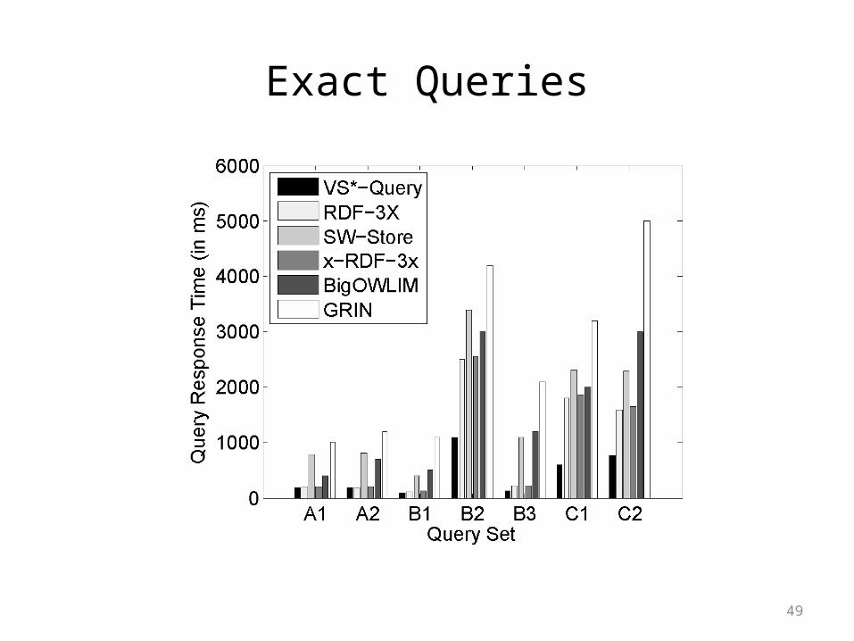
Exact Queries

49

Wildcard Queries

50

Outline





• Experiments

• Conclusions

51

Conclusions

• Vertex Encoding Technique;

• An Efficient index Structure: VS-tree;

• A Novel Filtering Technique.

52

53

Documents

GStore: Answering SPARQL Queries Via Subgraph Matching Lei Zou 1, Jinghui Mo 1, Lei Chen 2, M. Tamer Özsu 3, Dongyan Zhao 1 1 1 Peking University, 2 Hong