Growth Policy, Agglomeration, and (the Lack of)

Competition ∗

By Wyatt J. Brooks†, Joseph P. Kaboski‡, and Yao Amber Li §

Draft: April 28, 2016

Industrial clusters are generally viewed as good for growth and develop-

ment, but clusters can also enable non-competitive behavior. This paper

studies the presence of non-competitive pricing in geographic industrial

clusters. We develop, validate, and apply a novel identification strategy for

collusive behavior. We derive the test from the solution to a partial cartel

of perfectly colluding firms in an industry. Outside of a cartel, markups

depend on a firm’s market share but not on the total market share of firms

in the agglomeration, but in the cartel, markups across firms converge and

depend only on the overall market share of the agglomeration. Empirically,

we validate the test using plants with a common owner, and we then test

for collusion using data from Chinese manufacturing firms (1999-2009).

We find strong evidence for non-competitive pricing within a subset of in-

dustrial clusters, and we find the level of non-competitive pricing is roughly

four times higher in China’s “special economic zones”.

Both rich and poor countries generally regard industrial clusters as good for

productivity, growth, and development. The conventional economic wisdom dates

back to Marshall (1890), who cited three causes of natural industrial agglomera-

tion: geographic resources, demand concentrations, and local external economies

† University of Notre Dame. Email: wbrooks@nd.edu‡ University of Notre Dame and NBER. Email: jkaboski@nd.edu§ Hong Kong University of Science and Technology. Email: yaoli@ust.hk∗ Corresponding Author: Kaboski, Department of Economics, 717 Flanner Hall, Notre Dame, IN

46556. We are thankful for comments received Timo Boppart and participants in presentations at:Cornell University; the Federal Reserve Bank of Chicago; HKUST IEMS/World Bank Conference onUrbanization, Structural Change, and Employment; the London School of Economics/University Collegeof London; Princeton University; the University of Cambridge; and the World Bank.

1

of scale arising from thick input markets, thick labor markets, and/or technology

spillovers. Resource and demand concentrations often lead to efficient agglomera-

tion, but external economies leads to less than efficient agglomeration and act as

a justification for industrial policies fostering industrial clusters. Empirical evi-

dence supports Marshall’s hypotheses.1 Influential work, including Marshall, has

also viewed industrial clusters as productivity-enhancing through pro-competitive

pressures they may foster (e.g., Porter (1990)). Both advanced and developing

economies adopt policies that promote clusters.2

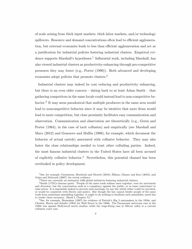
Industrial clusters may indeed be cost reducing and productivity enhancing,

but there is an even older concern – dating back to at least Adam Smith – that

gathering competitors in the same locale could instead lead to non-competitive be-

havior.3 It may seem paradoxical that multiple producers in the same area would

lead to noncompetitive behavior since it may be intuitive that more firms would

lead to more competition, but close proximity facilitates easy communication and

observation. Communication and observation are theoretically (e.g., Green and

Porter (1984), in the case of tacit collusion) and empirically (see Marshall and

Marx (2012) and Genesove and Mullin (1998), for example, which document the

behavior of actual cartels) associated with collusive behavior. They may also

foster the close relationships needed to trust other colluding parties. Indeed,

the most famous industrial clusters in the United States have all been accused

of explicitly collusive behavior.4 Nevertheless, this potential channel has been

overlooked in policy development.

1See, for example, Greenstone, Hornbeck and Moretti (2010), Ellison, Glaeser and Kerr (2010), andGuiso and Schivardi (2007), for recent evidence.

2There are currently an estimated 1400 global initiatives fostering industrial clusters.3Smith (1776)’s famous quote: “People of the same trade seldom meet together, even for merriment

and diversion, but the conversation ends in a conspiracy against the public, or in some contrivance toraise prices. It is impossible indeed to prevent such meetings, by any law which either could be executed,or would be consistent with liberty and justice. But though the law cannot hinder people of the sametrade from sometimes assembling together, it ought to do nothing to facilitate such assemblies; much lessto render them necessary. (Book I, Chapter X).”

4See, for example, Bresnahan (1987) for evidence of Detroit’s Big 3 automakers in the 1950s, andChristie, Harris and Schultz (1994) for Wall Street in the 1990s. The Paramount anti-trust case in the1940s was against Hollywood movie studios, while the wage-fixing case in Silicon valley is a currentcollusion court case.

2

This paper examines whether non-competitive behavior is associated with geo-

graphic concentration and therefore a potential cause for policy concern. Specifi-

cally, we define non-competitive behavior as behavior in either firm sales, hiring,

or purchases that internalizes pecuniary externalities on other firms. We make

three major contributions toward this end. First, we develop a novel, robust test

for identifying non-independent behavior for firms competing in the same indus-

try. Essentially, firms who are pricing independently internalize their own market

share but not the market shares of other firms when setting markups. In contrast,

firms in a cartel internalize the impact of their pricing on the other cartel firms, so

their markups depend on the aggregate market share of the cartel. Second, using

panel data on Chinese manufacturing firms, we validate that our test can identify

non-competitive behavior in sales using firms that are affiliates of the same par-

ent company as assumed “cartels”. Third, we show evidence of non-competitive

behavior at the level of industrial clusters in the Chinese economy. Although we

find limited levels of non-competitive behavior in the economy overall, the lev-

els within China’s “special economic zones” (SEZs) that are four times as high,

and the evidence for clusters pre-identified by the theory (i.e., those with little

cross-sectional variation in markups) are also quite high.

Our test is derived from a standard nested CES demand system with a finite

number of competing products and with a higher elasticity of substitution within

an industry than across industries. As is well known in this set up and empirically

confirmed (e.g., Atkeson and Burstein (2008),Edmond, Midrigan and Xu (2015)),

the gross markup that a firm charges is increasing in its market share. We show

that a subset of firms acting as a perfect cartel, and therefore maximizing joint

profits, leads to a convergence in markups across members, as each member’s

markup is set based on the total market share of the cartel firms rather than the

individual firms.

These results help us to identify non-competitive clusters in two ways. First,

they motivate our test of regressing a firm’s (inverse) markups on its own market

3

share and the total market share of its suspected or potential set of fellow cartel

members. Under perfectly independent pricing, only the coefficient on own mar-

ket share should be significant, while under perfect collusion, only the coefficient

on cartel market share should be significant. Moreover, according to the model,

the magnitudes of the two different coefficients in these two extreme cases ought

to be identical. Second, they suggest a way of pre-screening potentially collu-

sive industrial clusters by focusing on those with low cross-sectional variation in

markups across firms.

Our test is similar in spirit to Townsend (1994)’s now standard risk-sharing

regression, focusing on a cartel of local (colluding) firms rather than a syndicate

of local (risk-sharing) households. It has similar strengths, in that it allows for the

two extreme cases but also intermediate cases, and it allows us to be somewhat

agnostic about the actual details of non-competitive equilibrium. In principle,

collusion could be either explicit or tacit, for example, and firm behavior could be

Cournot or Bertrand. The test is also robust along other avenues. Importantly,

our theoretical results, and so the validity of the test, depend only on the constant

elasticity demand system. They are therefore robust to arbitrary assumptions on

the (differentiable) cost functions and geographical locations of the individual

firms. Moreover, using Monte Carlo simulations we show that the impacts of

uncertainty and correlated shocks on the results can be mitigated by firm and

region-time fixed effects.

Although both the substance of our question is of broad interest, and our meth-

ods are general, we apply our test to China. As the world’s largest growth miracle,

China is naturally of interest. The size of the Chinese country and economy give

us wide industrial and geographic heterogeneity. Moreover, promoting industrial

clusters has played a role in Chinese industrial policy, and both agglomeration

and markups have increased over time. Finally, we have a high quality panel of

firms: the Annual Survey of Chinese Industrial Enterprises (CIE) which contains

all state-owned enterprises (SOEs) and all larger non-state owned firms. From

4

this dataset, we utilized detailed data on revenue, capital, labor, firm location,

4-digit firm industry, and (for affiliates) parent firm for 162,000-411,000 firms over

the years, 1999-2009. The panel nature of the data is critical, allowing us to esti-

mate markups using the cost-minimization methods of De Loecker and Warzynski

(2012) and implement our test using within-firm variation.

Our test both identifies non-competitive pricing in simple validation exercises

and rejects it in simple placebo tests. Specifically, we test for joint profit max-

imization among groups of affiliates with the same parent company and in the

same industry. Similarly, we test for joint profit maximization among state-owned

firms in the same industry. Consistent with the theory, we estimate a highly sig-

nificant relationship between markups and cartel market share but an insignificant

relationship with own market share in our validation exercises. In our placebo

tests, we find no response in markups to industrial cluster market shares among

these sets of firms and no influence of SEZs on markup behavior.

We then use the broader sample of Chinese firms to examine our hypothesis

that firms in industrial clusters are more likely to collude. The overall sam-

ple of cluster shows that both own market share and total cluster market share

are significant predictors of markups, but the coefficient on own market share is

substantially larger. That is, competitive behavior appears more prevalent than

collusive behavior. In these analyses, however, the evidence for collusive behavior

is stronger, the smaller geographic definition of a cluster. We interpret this as

confirmation of the importance of proximity for collusion. Quantitatively, the

implied demand elasticities in all of our results are consistent in magnitude with

those found using other methods (e.g., elasticities based on international trade

patterns in Simonovska and Waugh (2014)).

We find stronger evidence in subsets of clusters, however. SEZs have policies

targeting firms in specific industries and locations for special treatment, foreign

partnerships, etc. but they also attempt to foster technological cooperation 5 We

5We use SEZ in the broad sense of the term. See Alder, Shao and Zilibotti (2013) for a summary of

5

find that the intensity of collusion is four times higher for clusters in SEZs than for

those not in SEZs. Our results are therefore of potentially normative importance

to evaluating the desirability of such policies in China and elsewhere. Moreover,

when we apply our pre-screening criteria, focusing on clusters in the lowest three

deciles of cross-sectional markup variation, and find that only the cluster market

share is a significant predictor of the panel variation in markups. That is, this

subsample appears to be dominated by effectively collusive behavior, and these

clusters are characterized by disproportionately higher concentration industries,

lower export intensities, and more private domestic enterprises as opposed to

foreign ventures or state-owned.

Finally, using various methods, we show that our tests do not appear to be

driven by spatially correlated shocks to demand or costs. Specifically, in a placebo

test, we construct clusters at a local level using state-owned firms that collude

more widely, and our test does not uncover spurious collusion. We also show that

our results robust to adding region-time fixed effects, or instrumenting for market

share using aggregators of other firms’ productivity.

Our paper contributes and complements the literatures on both industrial clus-

ters and collusion. We are not the first paper to examine collusion in an industrial

cluster or agglomeration. Bresnahan (1987) studied collusion of the Big 3 au-

tomakers in Detroit, and Christie, Harris and Schultz (1994) examine NASDAQ

collusion on Wall Street. More recently, Gan and Hernandez (2013) shows that

hotels near one another effectively collude. Methodologically, the recent indus-

trial organization literature on collusion has tended toward detailed case studies

of particular industries, making less stringent assumptions on demand or basing

them on deep institutional knowledge the industry.6 We complement these papers

by developing a test that can be applied to a wide range of industries and, rather

than focusing on a case study, applying the test to an entire economy, focusing

SEZs, their history, and their policies.6Einav and Levin (2010) give an excellent review of the rational for moving away from identification

based on cross-industry. Our test also relies on within-industry (indeed, within-firm) identification.

6

on a developing country that has actively promoted agglomeration. The local

growth impact of Chinese SEZs has been studied in Alder, Shao and Zilibotti

(2013), Wang (2013), and Cheng (2014), and they have found sizable positive

effects using panel level data at the local administrative units. Our firm level

evidence of non-competitive behavior suggests that this growth may have a po-

tential beggar-thy-neighbor element.7 This is consistent with the interpretation

that local governments fostered these SEZs, and that local growth success was

important to the careers of local politicians. Finally, we contribute to an emerg-

ing literature examining the role of firm competition – markups in particular –

on macro development, including Asturias, Garcia-Santana and Ramos (2015),

Edmond, Midrigan and Xu (2015), Galle (2016), and Peters (2015).

The rest of this paper is organized as follows. Section 2 presents the model

and derives the key theoretical results. Section 3 lays out are empirical test and

reviews our empirical application, including our data and methods for identifying

markups. Section 4 discusses the empirical results, while Section 5 concludes.

I. Model

We develop a simple static model of a finite number of differentiated firms

that yields relationships between firm markups and market shares under compe-

tition and cartel behavior, and we show the robustness of these results to various

assumptions. We assume a nested CES demand system of industries and vari-

eties within the industry, which we implicitly assume is independent of location.

Whereas the structure of demand is critical, we assume little about the production

side, allowing for a wide variety of determinants of firms costs, such as location

choice, arbitrary productivity spillovers and productivity growth for firms.8

7Nonetheless, in a second best world, collusion itself may be welfare improving. See, for example,Galle (2016) for the case where financial frictions are present.

8Our assumption that demand is independent of location implicilty assume low trade costs in output,which is important in allowing for agglomeration based on externalities rather than local demand. Wewill examine the empirical patterns with respect to tradability in Section 4.2.

7

A. Firm Demand

A finite number of firms operate in an industry i. The demand function of firm

n in industry i is:

(1) yin = Di

(pinPi

)−σ (PiP

)−γwhere pin represents the firm’s price, and Pi and P are the price indexes for

industry i and the economy overall, respectively. Thus, σ > 1 is the own price

elasticity of any variety within industry i, while γ > 1 is the elasticity of industry

demand to changes in the relative price index of the industry.9 Typically, σ > γ,

so that products are more substitutable within industries than industries are

with one another. The parameters Di captures overall demand at the industry

level. One could easily add a firm-specific component to this, but without loss of

generality we can also redefine the units so as to have demand symmetric across

firms. As each firm in the industry faces a symmetric demand, the industry price

index is price elasticity of an variety within industry i is :

(2) Pi =(∑

p1−σin

)1/(1−σ)

As we show in the appendix, this demand system can be derived as the solution

to a household’s problem that has nested CES utility.

One can invert the demand function to get the following inverse demand:

(3) pin = P

(yinYi

)−1/σ ( YiDi

)−1/γ

where:

Yi =

∑m∈Ωi

y1−1/σim

σσ−1

9We analyze disaggregated industries, so the assumption γ > 1 is natural.

8

To establish notation that will be used throughout this paper, we define market

shares as:

(4) sin =pinyin∑

m∈Ωi

pimyim=

y1−1/σin∑

m∈Ωi

y1−1/σim

where the second equality follows from substituting in (1) for prices and simpli-

fying. Our demand system implies that the cross-price elasticity is given by a

simple expression:

(5) ∀m 6= n,∂ log(yin)

∂ log(pim)= (σ − γ) sim

This will allow for simple aggregation in the results that follow. While our struc-

ture of demand is important, the constant elasticity of demand and this cross-price

elasticity restriction in particular, we allow for a very general specification of firm

costs. The cost to firm i of producing yin units of output is C(yin;Xin), where

Xin represents a general vector of characteristics Xin such as capital, technology,

location, etc. that are determined before production takes place. For example, a

special case of our model would be one in which an initial stage determines firm

placement among locations, and each firms’ productivity is determined by the

placement of each other firm.10

Now we separately consider the cases of firms acting independently and facing

a finite number of competitors, and a subset of firms in an industry forming a

cartel to maximize joint profits.

10The static nature of our pricing decision implicitly assumes that the vector Xin does not dependdirectly on past production decisions (e.g., no dynamic learning-by-doing or credit constraint considera-tions).

9

B. Firms Operating Independently

First we consider the case of all firms operate independently of one another.

The problem of a firm i in industry n is:

πin = maxyin

pinyin − C(yin;Xin)

Using (3), the firm’s optimal pricing condition equates marginal revenue with

marginal cost:

(6) pin

(σ − 1

σ+

[1

σ− 1

γ

]y

1−1/σin∑

m∈Ωny

1−1/σim

)= C ′(yin;Xin)

Using the definition of market shares sin given above, rearranging (6), and defining

the firm’s gross markup µin as the ratio of price to marginal cost yields the well-

known result:11

(7)1

µin=σ − 1

σ+

(1

σ− 1

γ

)sin

This equation implies that the only information that is needed to predict a firm’s

markup is that firm’s market share when the firm is operating independently.

For σ > γ, the empirically relevant case, additional sales that accompany lower

markups come more from substitution within the industry than from growing the

relative size of the industry itself. Firms with larger market shares have more

to lose by lowering their prices and therefore less to gain, so they charge higher

markups.

C. Cartel

We contrast the case of independent firms with one in which a group of firms

within an industry forms a cartel to maximize their joint profits. That is, within

11See, for example, Edmond, Midrigan and Xu (2015) or Atkeson and Burstein (2008).

10

industry i there is a set S ⊆ Ωi of firms that solve the following joint maximization

problem: ∑S

πin = maxyinn∈S

∑n∈S

pinyin − C(yin;Xin)

Using our definition of market shares again, we can express the first order condi-

tion as:

(8) ∀n ∈ S,C ′(yin;Xin) = pinσ − 1

σ+ pin

∑m∈S

(1

σ− 1

γ

)sim

Then rearranging (8) gives the relationship between markups and market shares:

(9)1

µin=σ − 1

σ+

(1

σ− 1

γ

)siS

where we have defined siS =∑

m∈S sim as the total market share of the cartel.

Under a cartel, the markup of a firm within the set S depends only on the total

market share of all firms within the group. The cartel internalizes the costs to its

own members of any one firm selling more goods, and these cost depends on the

total market shares of the member firms. A firm’s own market share influences its

markup only to the extent that it affects the cartel’s share. It is straightforward

to show that the pricing

Note a number of corollary results follow from equation (9). First, it is imme-

diately clear that firms within the cartel equalize their markups. Second, market

shares across cartel firms are more dissimilar than they are with independent

pricing, since under independent pricing, it is the larger share firms that charge

higher markups. Third, one can show that firms within a cartel charge higher

markups then they would under independent pricing. Fourth, a consequence of

this, given the high elasticity of substitution, σ > 1, is that each individual cartel

firm’s market share is lower under the cartel than under independent pricing. Fi-

nally, even the markups of non-cartel firms are somewhat higher than they would

be in the absence of a cartel; The non-cartel firms follow the independent markup

11

equation (7), but their share is higher, since the cartel firms’ shares are lower.

We summarize the above characterization in the following proposition.

PROPOSITION 1: Given σ > γ:

1) Under independent decisions, firm markups are increasing in the firm’s own

market share.

2) Under perfect cartel decisions, cartel firm markups are increasing in total

cartel market share, with the firm’s own market share playing no additional

role.

3) Firm markups are higher under perfect cartel decisions than independent

decisions.

4) Cartel firm markups are more similar under perfect cartel than independent

decisions.

5) Firm market shares are more dissimilar under perfect cartel decisions than

independent decisions.

Each of these claims will be addressed in our empirical work that follows. We

will use the first two claims to derive our test in Section 2, while the third and

fourth claims will be used to pre-identify potential collusive clusters. Finally, we

will use the fifth claim as an additional implication.

We have intentionally written Proposition 1 in general language. In the subsec-

tion below, we will show that, while the precise formulas vary, these more general

claims are robust to several alternative specifications.

D. Alternative Models

We present related results below for the cases of firm-specific price elasticities,

Bertrand competition rather than Cournot, and monopsonistic collusion.

12

Firm-specific price elasticities

To allow for markups to vary among competitive firms with the same market

share, we allow for a firm-specific elasticity of demand. In particular, suppose

that inverse demand takes the form:

pin = D1/γi Py

−1/σ+δinin Y

1/γ−1/σi

where now

Yi =

∑m∈Ωi

y1−1/σ+δimim

σσ−1

Here δin captures the firm-specific component of demand, and we think of these

as deviations from the average elasticity σ, i.e.,∑

n∈Ωiδin = 0. Proceeding as

before to derive markup equations, the first order conditions for an independent

firm imply:

(10)1

µin=σ − 1

σ+ δin +

(1

γ− 1

σ

)sin + δin

(σ

γ

γ − 1

σ − 1− 1

)sin

and for a cartel, the analogous equation is:

(11)1

µin=

(σ − 1

σ+ δin

)+

(1

γ− 1

σ

)∑m∈S

sim + δin

(σ

γ

γ − 1

σ − 1− 1

)∑m∈S

sim

Firm markup are again increasing in either the firm or cartel’s market share

and the magnitude of this relationship is government by the difference between

the within and across industry elasticities. In addition, however, the presence

of δin in the first time and second summation shows the level of markups are

firm-specific, even when market share is arbitrarily small or firms are members of

the same cartel. These differences are simply smaller under the cartel.

13

Bertrand competition

Now we consider the case where, when making production choices, firms take

competitors’ prices as given instead of quantities. From the demand function (1)

we can write the problem of a firm operating independently as:

maxpin,yin

pinyin − C(yin;Xin)

subject to: yin = Di

(pinPi

)−σ (PiP

)−γTaking first-order conditions with respect to both control variables and dividing

them yields the following analog to equations (7) and (9) are, respectively:

(12)µin

µin − 1= σ − (σ − γ)sin

and for the cartel

(13)µin

µin − 1= σ − (σ − γ)

∑m∈S

sim

Again, we see that firms markups are increasing in either the firm or cartel’s mar-

ket share and the magnitude of this relationship is government by the difference

between the within and across industry elasticities.

Monopsony behavior

Instead of colluding to increase prices of output, firms may instead collude to

reduce input costs. To consider this possibility, suppose all firms use a single

factor to produce their output by a production function yin = Fi(lin;Xin). To fix

ideas, and connect most closely with our empirical application, we refer to this as

labor. The supply of labor L depends on the market wage w, which is common

14

across firms. We assume it takes the following form:

w(L) = ALφ

Firms take the labor demand decisions of other firms (or those outside their own

cartel) as given. To isolate the effect of monopsony power here, in this case

suppose that firms take the price of their output as given. Then the problem of

an independent firm is:

maxyin,lin

pinyin − w(L)lin

subject to: yin ≤ Fi(lin;Xin)

Optimality for the independent firm implies that the markup is increasing in the

fraction of the market labor hired by the firm

(14) µin = 1 + φsL,in

and the analog for the cartel imply a result similar to (9):

(15) µin = 1 + φsL,in

Here sL,in ≡ lin/L and sL,in ≡∑m∈S

lim/L.

Two things are important to note, however. First, the expressions above de-

fine marginal cost as the cost of producing an additional unit at market prices.

Therefore the markup is:

µin =pin

w(L)/F ′i (lin;Xin)

Second, the shares in the expressions depend critically on the view of labor

markets and the definition of relevant labor supply, L. If labor is mobile across

industries but not across locations, it would be the total local labor force. If

15

labor is specialized by industry but mobile across locations, it would be the total

industry labor force. If immobile along both dimensions, it would be the total

local industry-specific labor, while if mobile in both dimensions, it would be the

total labor force overall.

II. Empirical Approach

In this section, we present our empirical test for non-competitive pricing and

discuss our application to China, including the data and methods of acquiring

markups.

A. Test for Non-Competitive Pricing

The model of the previous section yielded the result that the markups of com-

petitive firms depended on on the within-industry elasticity of demand and their

market share, while the markups of perfectly colluding firms depended on the

total market share of the firms in the cartel. This motivates the following single

empirical regression equation for inverse markups:

(16)1

µnit= αt + αni + β1snit + β2snjt + εnjit

for firm n, a member of (potential) cartel j, in industry i at time t.

In the case of purely independent pricing, the hypothesis would be β2 = 0, while

β1 < 0. While in the case of a pure cartel, we have the inverted hypothesis of β2 <

0, while β1 > 0. The relationships in equations (7) and (9) hold deterministically.

We interpret the error term εnjit as stemming from (classical) measurement error

in the estimation of markups, which we discuss in Section 3.3. We weight the

regressions by the number of firms in the industry, since measurement error in

markups should decrease in the number for firms.

Purely independent pricing and pure cartel represent two extreme cases, but

we can show that intermediate cases lead to intermediate values of our estimated

16

coefficients. In particular, define κ as the weight that the optimizing firm places

on other firms’ profits relative to its own, so that each firm maximizes:

πin + κ∑

m∈S−n

πim

It is easy to show that this leads to intermediate estimate of β1 and β2, where we

can solve for κ, σ, and γ using the following equations:

f =1

1 + β1/β2(1

µ

)avg

=σ − 1

σ+ β1savg + β2savg

β2/f =

(1

σ− 1

γ

)

An alternative interpretation of κ is to consider the case of a subset of S ⊂ S

firms perfectly colluding, while the others compete independently. This also leads

to intermediate estimates in both coefficients, with β1 larger and β2 smaller for

S than for S. (See Appendix for details.) Under somewhat stronger assumptions

that the distribution of market shares is the same for colluding and non-colluding

firms, we can show that κ the fraction of firms perfectly colluding, which we define

as κ (1− κ).

In general, the data may involve subsets of firms colluding to varying degrees

of course, but we view κ and these two lenses as a useful for considering the

magnitudes of our results.

Returning to equation (16), one sees strong parallels with the now-common,

risk-sharing test developed by Townsend (1994). In risk-sharing regressions,

household consumption is regressed on household income and total income in

the risk-sharing syndicate. Townsend solves the problem of a syndicate of house-

holds jointly maximizing utility and perfectly risk-sharing, and contrasts that

17

with households in financial autarky. We solve the problem of a syndicate of

firms jointly maximizing profits in perfect collusion and contrast with those in-

dependently maximizing profits. Townsend posited that households in proximity

are likely to be able to more easily cooperate, defining villages as the appropriate

risk-sharing network. We posit the same is true for firms and examine local coop-

eration of firms. Our test also shares another key strength of risk-sharing tests:

we don’t need to be explicit about the details of collusion because we only look

at its effects on pricing. It could be implicit or explicit price collusion, for exam-

ple. Moreover, collusion could be accomplished in many different ways, by firms

dividing up the market spatially, for example. Finally, as Section 2.3 illustrated,

firms could make decisions in Cournot or Bertrand fashion, and the essential test

would hold, although these lead to minor changes in the structural interpretation

of magnitudes.

We also note the presence of time and firm dummies in our rest. The time

dummies, αt capture time-specific variation, which is important since markups

have increased over time, as we show in the next section. In principle, firm-

specific fixed effects are not explicitly required, in the case of symmetric demand

elasticities.12 Nevertheless, we add αni to capture fixed firm-specific variation

in the markup. These allow for not only potential industry-specific variation

in demand elasticities (within industries) but also any firm-specific variation,

as in Section 2.4.1.13 Together, these time and firm controls assure that the

identification in the regression stems from within-firm, -cluster and -firm variation

over time in markups and market shares.

12Here the parallel with Townsend breaks, since risk-sharing regression require household fixed effects,or differencing, in order to account for household-specific Pareto weights. In contrast, cartels maximizeprofits rather than Pareto-weighted utility, and as long as profits can be freely transferred – an assumptionof a perfect cartel – all profits are weighted equally.

13The heterogeneity in the slope terms of equations (10) and (11) will show up in the error term of ourspecification. If the firm specific component δi is uncorrelated with either firm or cartel market share,the estimates of β1 and β2 will be unbiased. If instead it is correlated, the test of our hypotheses wherethe coefficients equal zero will still be valid – except for a knife edge case – but the structural estimatesof elasticities will be biased. See appendix.

18

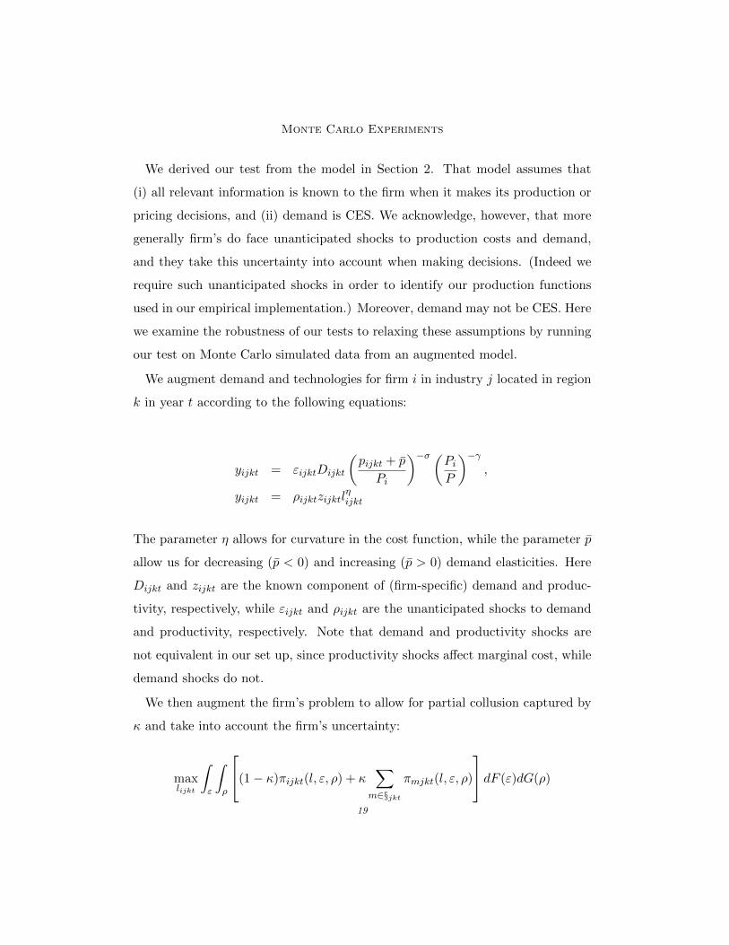
Monte Carlo Experiments

We derived our test from the model in Section 2. That model assumes that

(i) all relevant information is known to the firm when it makes its production or

pricing decisions, and (ii) demand is CES. We acknowledge, however, that more

generally firm’s do face unanticipated shocks to production costs and demand,

and they take this uncertainty into account when making decisions. (Indeed we

require such unanticipated shocks in order to identify our production functions

used in our empirical implementation.) Moreover, demand may not be CES. Here

we examine the robustness of our tests to relaxing these assumptions by running

our test on Monte Carlo simulated data from an augmented model.

We augment demand and technologies for firm i in industry j located in region

k in year t according to the following equations:

yijkt = εijktDijkt

(pijkt + p

Pi

)−σ (PiP

)−γ,

yijkt = ρijktzijktlηijkt

The parameter η allows for curvature in the cost function, while the parameter p

allow us for decreasing (p < 0) and increasing (p > 0) demand elasticities. Here

Dijkt and zijkt are the known component of (firm-specific) demand and produc-

tivity, respectively, while εijkt and ρijkt are the unanticipated shocks to demand

and productivity, respectively. Note that demand and productivity shocks are

not equivalent in our set up, since productivity shocks affect marginal cost, while

demand shocks do not.

We then augment the firm’s problem to allow for partial collusion captured by

κ and take into account the firm’s uncertainty:

maxlijkt

∫ε

∫ρ

(1− κ)πijkt(l, ε, ρ) + κ∑

m∈§jkt

πmjkt(l, ε, ρ)

dF (ε)dG(ρ)

19

where the unsubscripted ε, ρ, l are here vectors of demand shocks, cost shocks,

and labor input choices, respectively. Notice that F and G are probability distri-

butions over vectors. We will consider covariance of these shocks across firms at

the cluster, industry, and year levels by considering the impacts of different (e.g.,

cluster-year specific, industry-year specific) components.

We simulate this model for various parameter values, run our test regression

on the simulated data , and evaluate the parameters effects on our the bias of κ.

Full details are given in the appendix.

With respect to deviations from constant elasticity of demand, we find that

non-CES demand potentially impacts our estimates of the extent of collusion but

not our test for the presence of collusion. An increasing demand elasticity (where

demand becomes more elastic the more one sells) can lead to κ estimates that are

higher than the true κ, while decreasing demand elasticity can lead to κ estimates

lower than the true κ. However, these biases operate by biasing β1 but not β2.

Thus, our test β2 > 0 is still a valid test of the presence of collusion, and these

simulation results are strong evidence against the idea that deviations from CES

could lead to false positives, i.e., evidence for collusion where there is none. The

possibility of deviations from CES does add uncertainty to our interpretation of

ˆkappa, either understating or overstating the extent of collusion depending on the

direction of the deviation.

With respect to uncertainty, our findings are three fold. First, year and industry-

year demand and cost shocks do not bias our estimates test. Second, firm-year

demand and cost shocks bias our results downward. That is, our estimates under-

state the true level of kappa. The intuition here is that although the firm plans

to effectively sell according to the collusion rule, ex post because of the shocks it

deviates by either producing too much/little output or selling at a higher/lower

price.14 Third, region-year and region-industry-year shocks to costs and demand

14Marshall and Marx (2012) explain how correcting for such annual deviations, sometimes throughclandestine transfers, is an important part of sustaining explicit cartels.

20

bias our estimates upward. However, inclusion of region-year fixed effects elimi-

nates the bias from region-year specific cost shocks.

Given this third point, we want to guard against the possibility that we find

spurious evidence of collusion because of spatially correlated shocks. We address

this concern in multiple ways. One major way is by examining variation across dif-

ferent sets of firms, where we have stronger or weaker a priori reasons to suspect

collusion. First, we examine affiliated of the same parent company as a valida-

tion. Second, using similar reasoning, we evaluate firms that are state-owned

enterprises within an industry, and we also run a placebo test for local collusion

in the sample of state-owned firms. Third, we utilize the result in Proposition

1 that collusion makes markups more similar (Result 3) to motivate separately

examining industry-location clusters with low coefficients of variation in markups

over the cross-section of firms in the cluster. To limit potential endogeneity, we

identify these clusters using the cross-sectional variation of firms in the initial

year of our data (1999). Within the model, these clusters could have low markup

variation because (i) they are colluding or (ii) they have lower variation in market

shares (because of similarity in firm-specific demand or technology, for example).

We assume the former in our ex ante identification strategy, but then we evaluate

the latter ex post. Finally, as a robustness check, we add region-time specific fixed

effects to control for any region-time specific cost shocks (e.g., shocks to the costs

of land or labor).

B. Empirical Application

For our empirical test, we examine manufacturing firms in China. Manufac-

turing firms have the advantage of being highly tradable, and the assumption in

our model that demand does not depend on location or local markets is therefore

more appropriate. Our measurement methods are standard and closely follow the

existing literature.

21

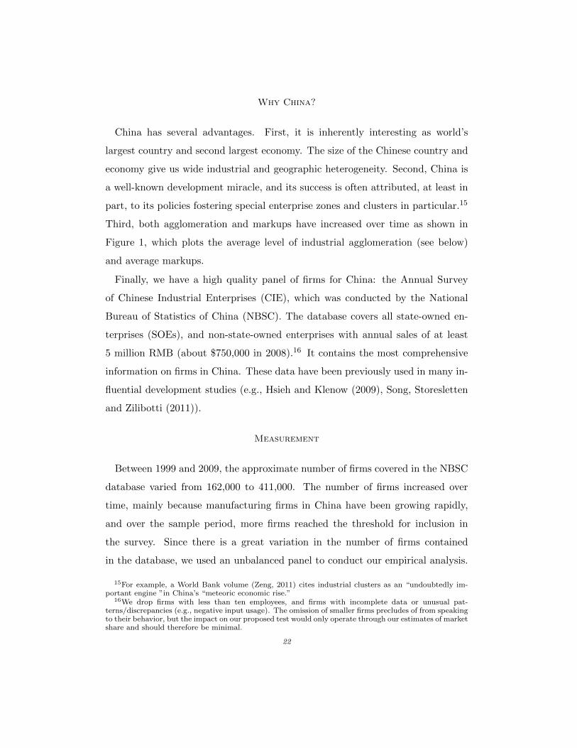
Why China?

China has several advantages. First, it is inherently interesting as world’s

largest country and second largest economy. The size of the Chinese country and

economy give us wide industrial and geographic heterogeneity. Second, China is

a well-known development miracle, and its success is often attributed, at least in

part, to its policies fostering special enterprise zones and clusters in particular.15

Third, both agglomeration and markups have increased over time as shown in

Figure 1, which plots the average level of industrial agglomeration (see below)

and average markups.

Finally, we have a high quality panel of firms for China: the Annual Survey

of Chinese Industrial Enterprises (CIE), which was conducted by the National

Bureau of Statistics of China (NBSC). The database covers all state-owned en-

terprises (SOEs), and non-state-owned enterprises with annual sales of at least

5 million RMB (about $750,000 in 2008).16 It contains the most comprehensive

information on firms in China. These data have been previously used in many in-

fluential development studies (e.g., Hsieh and Klenow (2009), Song, Storesletten

and Zilibotti (2011)).

Measurement

Between 1999 and 2009, the approximate number of firms covered in the NBSC

database varied from 162,000 to 411,000. The number of firms increased over

time, mainly because manufacturing firms in China have been growing rapidly,

and over the sample period, more firms reached the threshold for inclusion in

the survey. Since there is a great variation in the number of firms contained

in the database, we used an unbalanced panel to conduct our empirical analysis.

15For example, a World Bank volume (Zeng, 2011) cites industrial clusters as an “undoubtedly im-portant engine ”in China’s “meteoric economic rise.”

16We drop firms with less than ten employees, and firms with incomplete data or unusual pat-terns/discrepancies (e.g., negative input usage). The omission of smaller firms precludes of from speakingto their behavior, but the impact on our proposed test would only operate through our estimates of marketshare and should therefore be minimal.

22

This NBSC database contains 29 2-digit manufacturing industries and 425 4-digit

industries.17

The data also contain detailed data on revenue, fixed assets, labor, and, im-

portantly, firm location at the province, city, and county location. Of the three

designations, provinces are largest, and counties are smallest. We construct real

capital stocks by deflating fixed assets using investment deflators from China’s

National Bureau of Statistics and a 1998 base year. Finally, the “parent id code”,

which we use to identify affiliated firms, is only available for the year 2004, but we

assume that ownership is time invariant. We construct market shares using sales

data and following the definition in equation (4). We also use firms’ registered

designation to distinguish state-owned enterprises (SOEs) from domestic private

enterprises (DPEs), multinational firms (MNFs), and joint ventures (JVs).

We do not have direct measures of prices and marginal cost, so we cannot di-

rectly measure markups. Instead, we must estimate firm markups using structural

assumptions and structural methods, the method of De Loecker and Warzynski

(2012), referred to as DW hereafter, in particular. DW extend Hall (1987) to show

that one can use the first-order condition for any input that is flexibly chosen to

derive the firm-specific markup as the ratio of the factor’s output elasticities to

its firm-specific factor payment shares:

µi,t =θvi,tαxi,t

.

his structural approach has the advantage of yielding a plant-specific, rather than

a product-specific, markup. The result follows from cost-minimization and holds

for any flexibly chosen input where factor price equals the value of marginal

product. Importantly, we use materials as the relevant flexibly chosen factor.

The denominator αxi,t is therefore easily measured, though we follow DW in ad-

justing measured output Qi,t = Qi,texp(ui,t), by dividing by an estimate of the

17We use the adjusted 4-digit industrial classification from Brandt, Van Biesebroeck and Zhang (2012).

23

proportionate error term exp(uit).

The more difficult aspect is calculating the firm-specific output elasticity with

respect to materials, θvi,t, which requires estimating firm-specific production func-

tions. The issue is that inputs are generally chosen endogenously to productivity

(or profitability). We address this by applying Ackerberg, Caves and Frazer

(2006)’s methodology, presuming a 3rd-order translog gross output production

function in capital, labor, and materials that is:

(17) qnit = βk,iknit + βl,ilnit + βm,imnit+

βk2,ik2nit + βl2,il

2nit + βm2,im

2nit + βkl,iknitlnit + βkm,iknitmnit+

βlm,ilnitmnit + βk3,ik3nit + ...+ ωnit + εnit

Note that the coefficients vary across industry i but only the level of productiv-

ity is firm-specific. This firm-specific productivity has two stochastic components.

εnit is a shock that was unobserved/anticipated by the firm (and could reflect mea-

surement error) and is therefore exogenous to the firm’s input choices. However,

ωnit is a component of TFP that is observed/anticipated and so it is potentially

correlated with ki,t , lnit, and mnit, because the inputs are chosen endogenously

based on knowledge of the former. They assume that ωnit is Markovian and lin-

ear in ωni(t−1). Identification comes from orthogonality moment conditions that

stem from the timing of decisions, namely lagged labor and materials and current

capital (and their lags) are all decided before observing the innovation to the

TFP shock, and a two step procedure is used to first estimate εnit and then the

production function.

Production functions are estimated at the industry-level, although the estima-

tion allows for different factor neutral levels of productivity. The precision of

these estimates, and hence the measurement error in markups, therefore depends

on the number of firms in an industry. For this reason, we follow DW and weight

the data in our regressions using the total number of firms in the industry.

24

Finally, we use information on the geographic industries and clusters that we

study. Namely, we merge our geographic and industry data together with de-

tailed data from the China SEZs Approval Catalog (2006) on whether or not a

firm’s address falls within the geographic boundaries of targeted SEZ policies,

and, if so, when the SEZ started. We use the broad understanding of SEZs, in-

cluding both the traditional SEZs but also the more local zones such as High-tech

Industry Development Zones (HIDZ), Economic and Technological Development

Zones (ETDZ), Bonded Zones (BZ), Export Processing Zones (EPZ), and Bor-

der Economic Cooperation Zones (BECZ). Since no SEZs were added after 2006,

these data are complete. We also measure agglomeration at the industry level

using using the Ellison and Glaeser (1997) measure, where 0 indicates no geo-

graphic agglomeration (beyond that expected by industrial concentration), 1 is

complete agglomeration, and negative would indicate “excess diffusion” relative

to a random dartboard approach.18

Table 1 presents the relevant summary statistics for our sample of firms.

III. Results

We start by presenting the results validating our test using affiliated firms. We

then present the results for the overall sample (which are mixed), the results for

those pre-identified clusters with low variation in markups across firms (which

strongly indicate collusion), and some important characteristics of these collusive

clusters. Throughout our regression analysis, we report robust standard errors

18Specifically, start by defining a measure of geographic concentration, G:

G ≡∑i

(si − xi)2

where si is the share of industry employment in area i and xi is the share of total manufacturingemployment in area i. This therefore captures disproportionate concentration in industry i relative to

total manufacturing. Using the Herfindahl index H =∑Nj=1 z

2j , where zj is plant j’s share in total

industry employment, we have the following formula for the agglomeration index g:

g ≡G−

(1−

∑i x

2i

)H(

1−∑i x

2i

)(1−H)

25

clustered at the firm level.

A. Validation and Placebo Exercises

We start by running our test on our sample of affiliated firms. That is, we define

our potential cartels in equation (16) as groups of affiliated firms in the same in-

dustry who all have the same parent, and we construct the relevant market shares

of these cartels. We know from existing empirical work (e.g., Edmond, Midrigan

and Xu (2015)) that markups tend to be positively correlated with market share.

Our hypothesis is β1 = 0 and β2 < 0, however, so that own market share will

not impact markups after controlling for total market share. We estimate (16)

for various definition of industries: 2-digit, 3-digit, and 4-digit industries. Note

that the definition of industry affects not only the market share of the firm and

cartel, but the set of affiliates in the cartel. The broader industry classification

incorporates potential vertical collusion, but also makes market shares themselves

likely less informative.

Table 2 present the estimates, β1 and β2. (We omit the firm and time fixed

effects from the tables.) The first column shows the estimates, where we assume

perfectly independent behavior and constrain the coefficient on collusion share to

be zero. In the next three columns, we assume perfect collusion at the cluster level

(constraining the coefficient on firm share to be zero), and define clusters at the 2-,

3-, and 4-digit levels, respectively. The last three columns are analogous in terms

cluster definitions, but we do not constrain either coefficient. The standard errors

are robust standard errors, clustered at the firm level. the sample of observations

is a very small subset (less than two percent) of our full sample because we only

have parent/affiliate information for firms present in a subsample of firms in the

year (2004).

Focusing on the last three columns, we see that our hypothesis is confirmed

for the finer industry classifications, especially the 4-digit industry classification.

In particular, the coefficient on own share is small and statistically insignificant,

26

while the the cartel share is negative and marginally significant at a ten percent

level. Returning the results that constrain β1 to zero (i.e., column (iv)), and

applying (17), yields estimates of σ = 4.5 and γ = 2.9. (The corresponding values

implied by column 7 are very similar at 4.5 and 3.1.) For the 3-digit industry

classification, the impact of cartel market share is larger and even more significant,

but the coefficient on own share actually exceeds the coefficient on cartel share

(though statistically insignificant). The broad 2-digit industry classification gives

insignificant results, however, likely reflecting the fact that our test is based on

horizontal competition where industrial markets are narrowly defined.

Our second validation exercise is analogous. Instead of examining private af-

filiates owned by the same parent, however, we examine state-owned enterprises

(SOEs), which are all owned by the government. The variation in the data natu-

rally reflect the privatization process occurring in China over the period (declining

market share of SOEs), and the corresponding decrease in markups, but we hy-

pothesize that competition amongst SOEs is weaker than competition between

SOEs and private firms.

Indeed, the results in Table 3 verify this hypothesis. Columns 2-4 examine

collusion at different industry aggregations, and, once again, our test is consistent

with perfect collusion at the disaggregate industry level. In column 4, we find the

coefficient on own share to be insignificant at the 4-digit level, while the coefficient

on cluster’s share is negative and significant. While our test uncovers negative

and statistically significant coefficients on cluster’s share at the broader industry

levels too, own share is also significant and the implied κ values are tiny. Again,

our model is one of horizontal competition, so it is natural that the results are

most consistent when using the most disaggregate industries. For this reason, we

focus on the 4-digit industry classification, our narrowest, for the remainder of

our analyses.

Columns 5-7 consider variants where SOEs only collude with other SOEs (in

their 4-digit industry) that are in geographic proximity, i.e., at more local levels

27

of province, city, or county, respectively. We view this in some sense as a placebo

test, and indeed the evidence for collusion disappears at these more local levels.

The evidence for collusion weakens at these more local levels, and we take this

as evidence that the presence of any correlated local shocks are not enough to

erroneously lead to an assumption of local collusion in the case of SOEs.

Indeed, we run placebo tests that replicate are tests for industrial cluster-based

collusion but use these subsets of firms. We use the identical measure of industrial

cluster market share that we use below, but we only look at the markup response

for these sets of firms. The results are quit strong: we find no significant responses

of markups to the total market share of industrial clusters in either the SOE or

affiliated firm samples, and no effect of being in an SEZ. (See the Appendix for

full results.) Thus, our results do not seem to be driven by either the construction

of our data or spurious local correlations.

In sum, both validation tests are consistent with firms colluding within owner-

ship structures at the disaggregate industry level, and our test is able to reject

cluster-based collusion in placebo tests.

B. Non-Competitive Behavior in Industrial Clusters

We now turn to industrial clusters more generally by defining our potential

cartels as sets of firms in the same industry and geographic location. Table 4

presents the results. The first column shows the estimates, where we assume

perfectly independent behavior and constrain the coefficient on collusion share to

be zero. In the next three columns, we assume perfect collusion at the cluster

level (constraining the coefficient on firm share to be zero), and define clusters at

the province, city, and county level respectively. The next three columns allow

for both shares to influence inverse markups, while the final three interact firm

market share and cluster market share with an indicator variable for whether the

firm is in a SEZ. Again, we report robust standard errors clustered at the firm

level.

28

Focusing on columns 1 through 7, we note several strong results. First, all of

the estimates are highly significant indicating that both firm share and market

share are strongly related to markups. Because all estimates are statistically dif-

ferent from zero, we can rule out either perfectly independent behavior or perfect

collusion at the cluster level. Second, all the coefficients on market shares are

negative as we would predict if output within an industry are more substitutable

than output between industries. Third, the magnitudes are substantially larger

for own firm share. Fourth, as we define clusters at a more local level, the coef-

ficient on cluster share increases in magnitude, while the the coefficient on own

share decreases. This suggests that collusion is more prevalent among firms that

are local to one another.

The β2 < 0 estimates indicate some level of cluster-level collusion in the overall

sample.19 Again, applying equations (17), we can interpret the magnitude of the

implied elasticities and the extent of collusion. At the county level, we estimate

κ = 0.26, while we estimate just κ = 0.07 at the province level. This indicates a

relatively low level of non-competitive behavior overall, especially when examining

firms only located within the same province. The implied elasticity estimates are

σ = 4.8 and γ = 3.1. These implied elasticities are quite similar to those implied

in the smaller sample of affiliated firms, even though the level of collusion is

greater.

We turn to the role of SEZs examined in columns 8-10 of Table 4. The coeffi-

cients on the interaction of the SEZ dummy with firm market share are positive

and significant but smaller in absolute value than the coefficient on firm market

share itself. Adding the two coefficients, own market share is therefore a less

important a predictor of (inverse markups) in SEZs. Similarly, the coefficients

on cluster market share are negative, so that overall cluster market share is a

more important predictor in SEZs. Indeed, using the county-level estimates in

19We verify that this is not driven by the affiliated firms in two ways: (i) dropping the affiliated firmsfrom the sample, and (ii) assigning the parent group share within the cluster to firm share. Neitherchanges affect our results substantially.

29

the last column, we estimate a collusion index κ = 0.45 for firms within SEZs, four

times higher than that of firms not in SEZs, where κ = 0.11. Again, the results for

SEZs are strongest, the more local the definition of clusters. Recall, that SEZs are

essentially pro-business zones, combining tax breaks, infrastructure investment,

and government cooperation in order to attract investment. A common goal with

industry-specific zones or clusters is to foster technical coordination in order to

internalize productive externalities. The evidence suggests that such zones may

also facilitate marketing coordination and internalizing pecuniary externalities.

We have estimated similar regressions where we differentiate across industries

using the Rauch (1999) classification. Rauch classifies industries depending on

whether they sell homogeneous goods (e.g., goods sold on exchanges), referenced

priced goods, and differentiated goods. Without agriculture and raw materials,

our sample of homogeneous goods is limited, but we can distinguish between

industries that produce differentiated goods, and those that produce homoge-

nous/reference priced goods. Our estimates of κ are 0.14 for the former and

0.30 for the latter, indicating somewhat stronger collusion for more homogeneous

goods, consistent with existing arguments and evidence that collusion is less bene-

ficial and common in industries with differentiated products Dick (1996). Equally

interesting, the coefficients themselves are much larger for these goods, consistent

with a larger ρ, which would be expected, since goods should be highly substi-

tutable within these industries. (See appendix for details.) Again, we view this

latter consistency as further evidence that our results are driven by the pricing-

market share mechanism we highlight rather than some other statistical phe-

nomenon.

We have also examined robustness of the (county-level, unrestricted) results

in Table 4 to various alternative specifications. Although the theory motivates

weighting our regressions, neither the significance nor magnitudes of our re-

sults are dependent on the weighting in our regressions. We can also use the

Bertrand specification rather than Cournot, by replacing the dependent variable

30

with µnit/(µnit − 1). This Bertrand formulation require us to Windsorize the

data, however, because for very low markups the dependent variable explodes.

These observations take on huge weight, and very low markups are inconsistent

with the model for reasonable values of gamma. If we drop all observations be-

low 1.06, a lower bound on markups for a conservative estimate of γ = 10 (much

larger than implied by the Cournot estimates, for example), we get very similar

results, with implied elasticities σ = 5.5 and γ = 3.1 and the fraction colluding

f = 0.40. Finally, we can use log markup, rather than inverse markup, as our

dependent variable. The log function may make these regressions may be more

robust to very large outlier markups. Naturally, the predicted signs are reversed,

but they are both statistically significant, indicating partial collusion, and the

implied semi-elasticities with respect to own and cluster share are 9.7 and 3.6

percent, respectively. The details of these robustness studies are in our appendix.

We next turn to clusters which appear a priori likely to be potentially collusive

because they have low cross-sectional variation in markups. We do this by sorting

clusters into deciles according to their coefficient of variation of the markup. Table

5 presents the coefficient of variation of these deciles, along with other cluster

decile characteristics, when clusters are defined at the county level. Note that the

average markup increases with coefficient of variation of markups over the top

seven deciles, but that this pattern inverts for the lowest three deciles, where the

average markup is actually higher as the coefficient of variation decreases. Higher

markups and lower coefficients of variation may be more likely to be collusive,

given claims 2 and 3 in Proposition 1. We therefore focus on firms in the these

bottom three clusters, and the lowest thirty percent is not inconsistent with the

estimate that 26 percent of firms collude.20

The other key characteristics of these lowest deciles of clusters are also of inter-

est. First, although they have lower variation in markups, this does not appear

20These low markup variation deciles contain fewer firms on average, however, and so they constituteonly 16 percent of firms.

31

to be connected to lower variation in market shares, as the coefficients of varia-

tions in market shares are similar, showing no clear patterns across the deciles.

They have fewer firms per cluster, and are in industries with higher geographic

concentration (measured by the Ellison-Glaeser agglomeration index) and higher

industry concentration (as measured by the Hirschman-Herfindahl index). The

firms themselves are somewhat smaller in terms of fewer employees per firm.

Fewer firms in these clusters export, and overall exports are a lower fraction of

sales. Finally, although there are not sharp differences in the ownership distri-

bution, they are disproportionately domestic private enterprises and somewhat

less likely to be multi-national enterprises or joint ventures. In the appendix,

we include lists of the top 10 4-digit industries and top 10 cities that are most

overrepresented in the bottom three deciles.

Table 6 presents the results for this restricted sample of the lower three deciles.

The columns follow a parallel structure as in Table 4, but there are three columns

even for the regressions that only include firm market share because the set of

firms here varies depending on whether we define our clusters at the province,

city, or county level. Examining the results, in the results that assume perfectly

independent behavior we again find negative significant estimates at the province

and county level. (The city estimates have fewer observations, since there are

fewer firms in the low markup variation deciles of city clusters.) In the results, that

assume perfectly collusive behavior, we again find negative significant estimates

on cluster market share, and the results are again stronger, the more locally the

cluster is defined. The most interesting results in the table, however, are those

where we do constrain either coefficient. In this restricted sample, we again find

evidence of partially collusive behavior at the province level.

What is striking, however, is that the collusive behavior appears complete at lo-

cal levels within these restricted samples: only the estimates on beta2 are negative

and significant. The emphpositive β1 at the city and county level are admittedly

at odds with the theory, but the coefficient are not statistically significant. More-

32

over, the magnitude of the β1 (0.037) is less than half that of β2 (0.077) at the

county level. The county-level estimate in column (vi) implies a within-industry

elasticity σ that compares well with that in the full sample (5.0 vs. 4.8), but the

between-industry elasticity is somewhat higher than in the full sample (3.9 vs.

3.1).

Once again, we find significant impacts of SEZs when interacted with market

share. For counties, the region’s share is nearly twice as large for firms in SEZs.

C. Robustness

We now examine the robustness of our results to various alternatives. In par-

ticular, we attempt to address the issue that the correlation between markups

and cluster share may simply be driven by spatially correlated shocks to costs or

demand across firms, as our Monte Carlo simulations indicated could be prob-

lematic. We address this concern in two ways.

First, we add region-time specific fixed effects as controls into our regressions.

Our Monte Carlo simulations showed that these effectively control for any general

shocks or trends to production or costs at the region level, e.g., rising costs of land

or (non-industry-specific) labor from agglomeration economies. Controlling for

these, our regressions will only be identified by cross-industry variation in market

shares within a geographic location. Table 7 shows these results for the sample of

clusters with low initial variation in markups. The patterns are quite similar to

those in Table 6, although the magnitudes of the coefficients on cluster share are

somewhat smaller (e.g., -0.054 vs. -0.077) in column 9. The results are significant

at a five percent level. We find very similar results for the overall sample, but

since our SEZs show very little variation with counties, we cannot separately run

our SEZ test using these fixed effects. Nonetheless, we view the robustness of

our results as evidence that spatially correlated shocks (or trends) do not drive

our inference, although in principle, industry-specific spatially correlated shocks

could still play a role.

33

Second, we attempt an instrumental variable approach, since shares themselves

are endogenous. Identifying general instruments may be difficult, but in the

context of the model and our Ackerberg, Caves and Frazer (2006) estimation,

exogenous productivity shocks affect costs and therefore exogenously drive both

market share and markups. We motivate our instrument using an approximation,

the case of known productivity zin and monopolistic competition. This set up

yields the following relationship between shares and the distribution of produc-

tivity:

sin =pinyin∑

m∈Ωi

pimyim≈

z1−1/σin∑

m∈Ωi

z1−1/σim

We construct instruments for own market share (I1) and cluster market share

(I2) using variants of the above formula that exclude the firm’s own productivity

and the productivities of all firms in the firm’s cluster (Sn), respectively:

I1 =1∑

m∈Ωi/n

z1−1/σim

,

I2 =1∑

m∈Ωi/Sn

z1−1/σim

This two-stage estimation yields very similar results (see Appendix for details).

For example, the coefficient on cluster share in the analog to column (ix) is -0.050

and is significant at the five percent level. Again, the patterns we develop are

broadly robust.

In sum, we have shown that: the test detects collusion among firms owned by

the same parents in the affiliated and SOE samples; the markups of local SOEs

in a placebo test do not respond to their cluster market share; the estimates are

consistent with the model’s mechanism based on the Rauch classification; our

collusion patterns are stronger in SEZs; the collusion patterns are very strong in

clusters that the model pre-identifies as likely colluders; these collusion patterns

34

are robust to inclusion of time-region specific fixed effects and instrumenting for

market share.

IV. Conclusion

We have developed a simple yet fairly robust test for identifying non-competitive

behavior for subsets of firms competing in the same industry. Using this test we

have found evidence of collusion in Chinese industrial clusters. These results are

strongest within narrowly-defined clusters in terms of narrow industries and nar-

row geographic units. A minority but non-negligible share of firms and clusters

appear to suffer from from non-competitive behavior, and these are dispropor-

tionately so – four times as strong – in special economic zones.

The results open several avenues for future research. We have focused on China.

However, the fact that it satisfied our validation exercises means it could easily

applied more generally to other countries and contexts where firm panel data are

available. Finally, the potential normative importance of our results are com-

pelling with respect to evaluating cluster promoting industrial policies, such as

local tax breaks, subsidized credit, or targeted infrastructure investments. They

motivate more rigorous evaluation of various normative considerations including:

weighing extent to which cartels hurt (or perhaps even help) consumers; produc-

tivity gains from external economies of scale vs. monopoly pricing losses from

cartels; and local vs. global welfare implications and incentives. Precisely these

issues are the subject of our current research.

REFERENCES

Ackerberg, Daniel, Kevin Caves, and Garth Frazer. 2006. “Structural

identification of production functions.” University Library of Munich, Germany

MPRA Paper 38349.

Alder, Simon, Lin Shao, and Fabrizio Zilibotti. 2013. “The Effect of Eco-

nomic Reform and Industrial Policy in a Panel of Chinese Cities.” Working

35

Paper.

Asturias, Jose, Manuel Garcia-Santana, and Roberto Ramos. 2015.

“Competition and the Welfare Gains from Transportation Infrastructure: Evi-

dence from the Golden Quadrilateral in India.” Working Paper.

Atkeson, Andrew, and Ariel Burstein. 2008. “Pricing-to-Market, Trade

Costs, and International Relative Prices.” American Economic Review,

98: 1998–2031.

Brandt, Loren, Johannes Van Biesebroeck, and Yifan Zhang. 2012. “Cre-

ative Accounting or Creative Destruction? Firm-level Productivity Growth in

Chinese Manufacturing.” Journal of Development Economics, 97(2): 339–351.

Bresnahan, Timothy. 1987. “Competition and Collusion in the American Au-

tomobile Industry: The 1955 Price War.” Journal of Industrial Economics,

35(4): 457–482.

Cheng, Yiwen. 2014. “Place-Based Policies in a Development Context - Evi-

dence from China.” Working Paper.

Christie, William, Jeffrey Harris, and Paul Schultz. 1994. “Why did NAS-

DAQ Market Makers Stop Avoiding Odd-Eighth Quotes?” Journal of Finance,

49(5): 1841–1860.

De Loecker, Jan, and Frederic Warzynski. 2012. “Markups and Firm-Level

Export Status.” American Economic Review, 102(6): 2437–71.

Dick, Andrew. 1996. “When are Cartels Stable Contracts?” Journal of Law

and Economics, 39(1): 241–283.

Edmond, Chris, Virgiliu Midrigan, and Daniel Xu. 2015. “Competition,

Markups and the Gains from International Trade.” American Economic Review.

Einav, Liran, and Jonathan Levin. 2010. “Empirical Industrial Organization:

A Progress Report.” Journal of Economic Perspectives, 24(2): 145–162.

36

Ellison, Glenn, and Edward L Glaeser. 1997. “Geographic Concentration in

U.S. Manufacturing Industries: A Dartboard Approach.” Journal of Political

Economy, 105(5): 889–927.

Ellison, Glenn, Edward Glaeser, and William Kerr. 2010. “What Causes

Industrial Agglomeration? Evidence from Coagglomeration Patterns.” Ameri-

can Economic Review, 100(3): 1195–1213.

Galle, Simon. 2016. “Competition, Financial Constraints and Misallocation:

Plant-Level Evidence from Indian Manufacturing.” Working Paper.

Gan, Li, and Manuel Hernandez. 2013. “Making Friends with Your Neigh-

bors? Agglomeration and Tacit Collusion in the Lodging Industry.” Review of

Economics and Statistics, 95(3): 1002–1017.

Genesove, David, and Wallace Mullin. 1998. “Testing Static Oligopoly Mod-

els: Conduct and Cost in the Sugar Industry, 1890-1914.” RAND Journal of

Economics, 29(2): 355–377.

Green, Edward, and Robert Porter. 1984. “Noncooperative Collusion under

Imperfect Price Information.” Econometrica, 52(1): 87–100.

Greenstone, Michael, Rick Hornbeck, and Enrico Moretti. 2010. “Iden-

tifying Productivity Spillovers: Evidence from Winners and Losers of Large

Plant Openings.” Journal of Political Economy, 118(3): 536–598.

Guiso, Luigi, and Fabiano Schivardi. 2007. “Spillovers in Industrial Distric-

trs.” Economic Journal, 117(516): 68–93.

Hall, Robert. 1987. “Productivity and the Business Cycle.” Carnegie-Rochester

Conference Series on Public Policy, 27: 421–444.

Hsieh, Chang-Tai, and Peter Klenow. 2009. “Misallocation and Manufactur-

ing TFP in China and India.” Quarterly Journal of Economics, 124(4): 1403–

1448.

37

Marshall, Alfred. 1890. Principles of Economics. London: MacMillan.

Marshall, Robert, and Leslie Marx. 2012. The Economics of Collusion. MIT

Press.

Peters, Michael. 2015. “Heterogeneous Mark-Ups, Growth and Endogenous

Misallocation.” Working Paper.

Porter, Michael. 1990. The Competitive Advantage of Nations. Free Press, New

York.

Rauch, James E. 1999. “Networks Versus Markets in International Trade.”

Journal International of Economics, 48(1): 7–35.

Simonovska, Ina, and Michael Waugh. 2014. “Elasticity of Trade: Estimates

and Evidence.” Journal of International Economics, 92(1): 34–50.

Smith, Adam. 1776. The Wealth of Nations. W. Strahan and T. Cadell, London.

Song, Zheng, Kjetil Storesletten, and Fabrizio Zilibotti. 2011. “Growing

Like China.” American Economic Review, 101(1): 202–241.

Townsend, Robert. 1994. “Risk and Insurance in Village India.” Econometrica,

62(3): 539–591.

Wang, Jin. 2013. “The economic impact of Special Economic Zones: Evidence

from Chinese municipalities.” Journal of Development Economics, 101: 133–

147.

Zeng, Douglas. 2011. “How Do Special Economic Zones and Industrial Clus-

ters Drive China’s Rapid Development?” In Building Engines for Growth and

Competitiveness in China. , ed. Douglas Zeng. Washington, D.C.

38

Figure 1: Increasing Agglomeration and Markups over Time in China

0.0

1.0

2.0

3.0

4.0

5.0

6.0

7.0

8E

-G A

gglo

mer

atio

n

1999 2001 2003 2005 2007 2009year

County

City

Province

11.

051.

11.

151.

21.

251.

31.

35G

ross

Mar

kup

1999 2001 2003 2005 2007 2009Year

Markup Level (weighted)

Markup Level (unweighted)

Table 1: Key Summary Statistics of Data

Variable Mean Median S.D. Min Max

Markup 1.29 1.26 0.21 0.61 4.76

Firm Share 0.00 0.00 0.01 0 1Cluster Share (Province) 0.14 0.10 0.14 0 1

Cluster Share (City) 0.04 0.02 0.06 0 1Cluster Share (County) 0.02 0.00 0.04 0 1

Capital per Firm 322.85 48.17 3719.52 0.01 1035383.00Materials per Firm 719.09 167.95 5944.99 0.05 860549.30

Real Output per Firm 998.76 243.45 7967.81 0.08 1434835.00Workers per Firm 287.82 120 1005.62 10 166857

No. of Firms 408,848

Notes: Market shares are computed using 4-digit industries. Capital,output and materials are in thousand RMB (in real value).

Table 2: Baseline Results Using Affiliated Firms

Dependent Variable: 1µnit

(1) (2) (3) (4) (5) (6) (7)4-digit 2-digit 3-digit 4-digit 2-digit 3-digit 4-digit

Firm’s share -0.036 -0.223 0.283 0.073(0.057) (0.666) (0.268) (0.086)

Cluster’s share -0.206 -0.196∗∗ -0.077 -0.190 -0.258∗∗∗ -0.119∗

(0.171) (0.090) (0.049) (0.182) (0.100) (0.072)

Year FEs YES YES YES YES YES YES YES

Firm FEs YES YES YES YES YES YES YES

Observations 26779 26779 26779 26779 26779 26779 26779

Adjusted R2 .518 .518 .519 .518 .518 .519 .518

Notes: Robust standard errors clustered at firm level in parentheses. Significance: ∗∗∗: 1%, ∗∗:5%, ∗: 10%. Various industry aggregation levels are employed, including 4-digit industry (inspecifications 1, 4 and 7), 3-digit industry (in specifications 3 and 6), and 2-digit industry (inspecifications 2 and 5). All specifications are regressions weighted by the number of observationsfor each two-digit CIC sector production function estimation reported (following De Loecker et al.2014). All regressions include a constant term.

Table 3: Baseline Results Using SOEs as Cluster

Dependent Variable: 1µnit

(1) (2) (3) (4) (5) (6) (7)all SOEs in the industry province city county

4-digit 2-digit 3-digit 4-digit 4-digit 4-digit 4-digit

Firm’s Share -2.188∗∗ -2.055∗∗ -0.369∗ -0.034 0.005 -0.006 -0.048(0.854) (0.860) (0.220) (0.059) (0.067) (0.077) (0.130)

Cluster’s Share -0.046∗∗ -0.019∗∗ -0.026∗∗∗ -0.060∗ -0.048 -0.007(0.019) (0.010) (0.007) (0.032) (0.049) (0.115)

Year FEs YES YES YES YES YES YES YES

Firm FEs YES YES YES YES YES YES YES

Observations 111520 111520 111520 111520 111520 111520 111520

Adjusted R2 .572 .572 .572 .572 .572 .572 .572

Notes: Robust standard errors clustered at firm level in parentheses. Significance: ∗∗∗: 1%, ∗∗:5%, ∗: 10%. Various industry aggregation levels are employed, including 4-digit industry (inspecifications 1 and 4-7), 3-digit industry in specifications, and 2-digit industry in specifications 2.All specifications are regressions weighted by the number of observations for each two-digit CICsector production function estimation reported (following De Loecker et al. 2014). All regressionsinclude a constant term.

Tab

le4:

Bas

elin

eR

esult

sU

sing

Ove

rall

Sam

ple

Dep

end

ent

Var

iab

le:

1µnit

(1)

(2)

(3)

(4)

(5)

(6)

(7)

(8)

(9)

(10)

Pro

vin

ceC

ity

Cou

nty

Pro

vin

ceC

ity

Cou

nty

Pro

vin

ceC

ity

Cou

nty

Fir

m’s

Sh

are

-0.1

12∗∗

∗-0

.104

∗∗∗

-0.0

86∗∗

∗-0

.081

∗∗∗

-0.1

57∗∗

∗-0

.142

∗∗∗

-0.1

42∗∗

∗

(0.0

21)

(0.0

21)

(0.0

21)

(0.0

22)

(0.0

27)

(0.0

28)

(0.0

28)

Reg

ion

’sS

har

e-0

.011

∗∗∗

-0.0

31∗∗

∗-0

.041

∗∗∗

-0.0

09∗∗

∗-0

.024

∗∗∗

-0.0

29∗∗

∗-0

.003

-0.0

17∗∗

∗-0

.017

∗∗

(0.0

02)

(0.0

04)

(0.0

06)

(0.0

02)

(0.0

05)

(0.0

07)

(0.0

03)

(0.0

05)

(0.0

08)

SE

Z*F

irm

’sS

har

e0.

073∗

0.08

6∗∗

0.09

0∗∗

(0.0

40)

(0.0

41)

(0.0

42)

SE

Z*R

egio

n’s

Sh

are

-0.0

12∗∗

∗-0

.022

∗∗∗

-0.0

26∗∗

(0.0

04)

(0.0

07)

(0.0

11)

SE

ZD

um

my

0.00

10.

001

-0.0

00(0

.001

)(0

.001

)(0

.001

)

Yea

rF

Es

YE

SY

ES

YE

SY

ES

YE

SY

ES

YE

SY

ES

YE

SY

ES

Fir

mF

Es

YE

SY

ES

YE

SY

ES

YE

SY

ES

YE

SY

ES

YE

SY

ES

Ob

serv

atio

ns

1470

892

1470

892

1470

892

1470

892

1470

892

1470

892

1470

892

1205

337

1205

337

1205

337

Ad

just

edR

20.

541

0.54

10.

541

0.54

10.

541

0.54

10.

541

0.53

80.

538

0.53

8

Note

s:R

obust

standard

erro

rscl

ust

ered

atfirm

leve

lin

pare

nth

eses

.Sig

nifi

cance

:∗∗

∗ :1%

,∗∗

:5%

,∗ :

10%

.R

egio

ns

are

defi

ned

at

vari

ous

aggre

gati

on

leve

ls,

incl

udin

gpro

vin

ce(i

nsp

ecifi

cati

ons

2,5,

and

8),

city

(in

spec

ifica

tions

3,6,

and

9),

and

county

(in

spec

ifica

tion

s4,

7,

and

10)

.A

llsp

ecifi

cati

ons

are

regr

essi

ons

wei

ghte

dby

the

num

ber

of

obse

rvat

ions

for

each

two-

dig

itC

ICse

ctor

pro

duct

ion

funct

ion

esti

mati

on

rep

ort

ed(f

ollow

ing

De

Loec

ker

etal.

2014)

.A

llre

gre

ssio

ns

incl

ude

aco

nst

ant

term

.

Tab

le5:

Clu

ster

Char

acte

rist

ics

by

Clu

ster

Dec

ile

ofC

oeffi

cien

tof

Var

iati

onof

Mar

kup

Clu

ster

Ind

ust

ryC

once

ntr

atio

nF

irm

Fir

mO

wn

ersh

ipD

ecil

eof

Avg.

Loca

lC

omp

etit

ion

Ind

icat

orC

har

acte

rist

ics

Exp

orti

ng

Dis

trib

uti

onC

oeffi

cien

tC

oeffi

cien

tA

vg.

Coeffi

cien

tA

vg.

EG

Hir

sch

man

-A

vg.

Mea

nA

vg.

Avg.

Avg.

ofV

aria

tion

ofV

aria

tion

Avg.

ofV

aria

tion

ofA

vg.

Fir

ms

Agg

lom

erat

ion

Her

find

ahl

Exp

ort

Per

cent

Per

cent

Per

cent

ofM

arku

pof

Mar

ku

pM

ean

Mar

ku

pM

arke

tS

har

eP

erC

lust

erIn

dex

Ind

exS

har

eD

PE

FIE

SO

E

10.

011.

224

4.3

1.69

0.01

020.

023

0.16

7914

72

0.03

1.22

34.

32.

220.

0100

0.02

00.

1481

145

30.

041.

223

4.5

2.92

0.00

990.

018

0.16

8114

4

40.

061.

219

4.4

3.72

0.01

000.

017

0.19

7917

45

0.08

1.22

54.

44.

350.

0098

0.01

70.

2279

184

60.

091.

232

4.9

4.70

0.00

990.

017

0.24

7521

47

0.11

1.23

44.

44.

990.

0100

0.01

60.

2370

254

80.

141.

252

5.5

5.03

0.00

960.

018

0.28

6233

59

0.17

1.28

05.

04.

570.

0095

0.01

80.

2957

376

100.

261.

345

4.5

3.27

0.00

950.

022

0.20

5434

12

Tab

le6:

Bas

elin

eR

esult

sU

sing

Low

CV

Dec

iles

Dep

end

ent

Var

iab

le:

1µnit

(1)

(2)

(3)

(4)

(5)

(6)

(7)

(8)

(9)

Pro

vin

ceC

ity

Cou

nty

Pro

vin

ceC

ity

Cou

nty

Pro

vin

ceC

ity

Cou

nty

Fir

m’s

shar

e-0

.072

∗-0

.002

-0.0

40-0

.060

0.02

70.

037

(0.0

44)

(0.0

64)

(0.0

35)

(0.0

44)

(0.0

64)

(0.0

43)

Reg

ion

’ssh

are

-0.0

14∗∗

-0.0

24-0

.059

∗∗∗

-0.0

12∗∗

-0.0

28∗

-0.0

77∗∗

∗

(0.0

06)

(0.0

16)

(0.0

22)

(0.0

06)

(0.0

14)

(0.0

25)

Yea

rF

Es

YE

SY

ES

YE

SY

ES

YE

SY

ES

YE

SY

ES

YE

S

Fir

mF

Es

YE

SY

ES

YE

SY

ES

YE

SY

ES

YE

SY

ES

YE

S

Ob

serv

atio

ns

2714

0315

9353

1920

6827

1403

1593

5319

2068

2714

0315

9353

1920

68

Ad

just

edR

20.

570.

713

0.84

10.

570.

713

0.84

10.

570.

713

0.84

1

Note

s:R

obust

stan

dar

der

rors

clust

ered

atfirm

leve

lin

pare

nth

eses

.Sig

nifi

cance

:∗∗

∗ :1%

,∗∗

:5%

,∗ :

10%

.R

egio

ns

are

defi

ned

at

vari

ous

aggre

gati

on

leve

ls,

incl

udin

gpro

vin

ce(i

nsp

ecifi

cati

ons

1,4,

and

7),

city

(in

spec

ifica

tion

s2,

5,

and

8),

and

county

(in

spec

ifica

tions

3,6

and

9).

All

spec

ifica

tion

sar

ere

gres

sion

sw

eighte

dby

the

num

ber

of

obse

rvat

ions

for

each

two-

dig

itC

ICse

ctor

pro

duct

ion

funct

ion

esti

mat

ion

rep

ort

ed(f

ollo

win

gD

eL

oec

ker

etal

.20

14).

All

regre

ssio

ns

incl

ude

aco

nst

ant

term

.

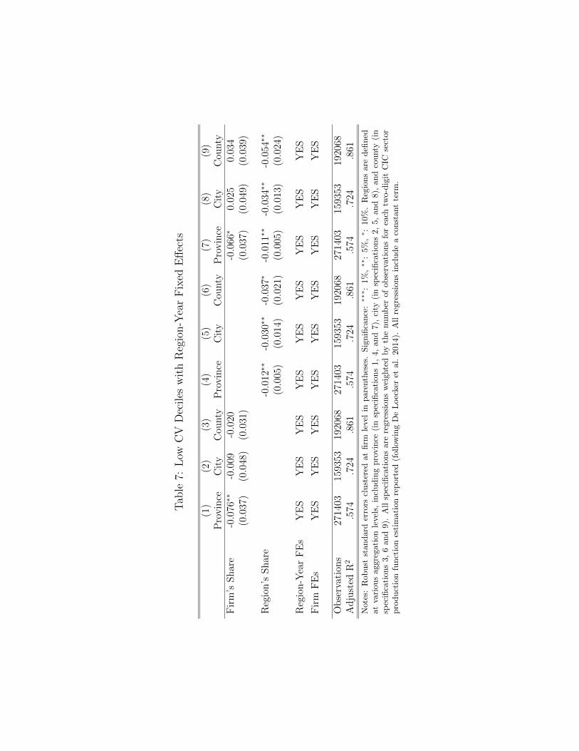
Tab

le7:

Low

CV

Dec

iles

wit

hR

egio

n-Y

ear

Fix

edE

ffec

ts

(1)

(2)

(3)

(4)

(5)

(6)

(7)

(8)

(9)

Pro

vin

ceC

ity

Cou

nty

Pro

vin

ceC

ity

Cou

nty

Pro

vin

ceC

ity

Cou

nty

Fir

m’s

Sh

are

-0.0

76∗∗

-0.0

09-0

.020

-0.0

66∗

0.02

50.

034

(0.0

37)

(0.0

48)

(0.0

31)

(0.0

37)

(0.0

49)

(0.0

39)

Reg

ion

’sS

har

e-0

.012

∗∗-0

.030

∗∗-0

.037

∗-0

.011

∗∗-0

.034

∗∗-0

.054

∗∗

(0.0

05)

(0.0

14)

(0.0

21)

(0.0

05)

(0.0

13)

(0.0

24)

Reg

ion

-Yea

rF

Es

YE

SY

ES

YE

SY

ES

YE

SY

ES

YE

SY

ES

YE

S

Fir

mF

Es

YE

SY

ES

YE

SY

ES

YE

SY

ES

YE

SY

ES

YE

S

Ob

serv

atio

ns

2714

0315

9353

1920

6827

1403

1593

5319

2068

2714

0315

9353

1920

68A

dju

sted

R2

.574

.724

.861

.574

.724

.861

.574

.724

.861

Note

s:R

obust

stan

dar

der

rors

clust

ered

atfirm

leve

lin

pare

nth

eses

.Sig

nifi

cance

:∗∗

∗ :1%

,∗∗

:5%

,∗ :

10%

.R

egio

ns

are

defi

ned

at

vari

ous

aggre

gati

on

leve

ls,

incl

udin

gpro

vin

ce(i

nsp

ecifi

cati

ons

1,4,

and

7),

city

(in

spec

ifica

tion

s2,

5,

and

8),

and

county

(in

spec

ifica

tions

3,6

and

9).

All

spec

ifica

tion

sar

ere

gres

sion

sw

eighte

dby

the

num

ber

of

obse

rvat

ions

for

each

two-

dig

itC

ICse

ctor

pro

duct

ion

funct

ion

esti

mat

ion

rep

ort

ed(f

ollo

win

gD

eL

oec

ker

etal

.20

14).

All

regre

ssio

ns

incl

ude

aco

nst

ant

term

.

Table A.1: Appendix Table–Robustness

(1) (2) (3) (4) (5) (6) (7) (8)

Panel A: Dependent Variable = 1/µnit

Firm’s Share -0.112∗∗∗ -0.081∗∗∗ -0.142∗∗∗ -0.049∗∗∗ -0.031∗∗∗ -0.073∗∗∗

(0.011) (0.012) (0.015) (0.009) (0.010) (0.013)

Region’s Share -0.041∗∗∗ -0.029∗∗∗ -0.017∗∗∗ -0.023∗∗∗ -0.017∗∗∗ -0.002(0.004) (0.004) (0.005) (0.004) (0.005) (0.005)

SEZ*Firm’s Share 0.090∗∗∗ 0.076∗∗∗

(0.023) (0.021)

SEZ*Region’s Share -0.026∗∗∗ -0.032∗∗∗

(0.007) (0.007)

Observations 1470892 1470892 1470892 1205337 1470892 1470892 1470892 1205337Adjusted R2 0.541 0.541 0.541 0.538 0.539 0.539 0.539 0.536

Panel B: Dependent Variable = µnit/(µnit − 1) (full sample)

Firm’s Share 169.961 143.820 295.045 352.320 329.188 605.930(256.601) (280.289) (364.181) (346.765) (390.900) (530.172)

Region’s Share 45.849 24.251 16.686 89.076 22.092 11.689(95.777) (104.618) (123.835) (152.865) (172.321) (217.461)

SEZ*Firm’s Share -300.513 -547.209(562.327) (842.053)

SEZ*Region’s Share 24.188 29.639(164.433) (305.981)

Observations 1470892 1470892 1470892 1205337 1470892 1470892 1470892 1205337Adjusted R2 -0.021 -0.021 -0.021 -0.068 -0.068 -0.068 -0.068 -0.098

Panel C: Dependent Variable = µnit/(µnit − 1) (drop µnit < 1.06)

Firm’s Share -2.482∗∗∗ -1.429∗∗∗ -3.048∗∗∗ -1.724∗∗∗ -0.958∗∗∗ -2.077∗∗∗

(0.322) (0.352) (0.462) (0.284) (0.318) (0.406)

Region’s Share -1.185∗∗∗ -0.971∗∗∗ -0.842∗∗∗ -0.913∗∗∗ -0.726∗∗∗ -0.473∗∗∗

(0.120) (0.131) (0.156) (0.122) (0.137) (0.163)

SEZ*Firm’s Share 2.937∗∗∗ 2.693∗∗∗

(0.716) (0.649)

SEZ*Region’s Share -0.445∗∗ -0.677∗∗∗

(0.204) (0.226)

Observations 1335576 1335576 1335576 1093555 1335576 1335576 1335576 1093555Adjusted R2 0.438 0.438 0.438 0.439 0.432 0.432 0.433 0.434

Panel D: Dependent Variable = log(mu)nit

Firm’s Share 0.136∗∗∗ 0.097∗∗∗ 0.171∗∗∗ 0.057∗∗∗ 0.035∗∗ 0.087∗∗∗

(0.014) (0.016) (0.020) (0.012) (0.014) (0.017)

Region’s Share 0.051∗∗∗ 0.036∗∗∗ 0.016∗∗ 0.028∗∗∗ 0.021∗∗∗ -0.001(0.005) (0.006) (0.007) (0.005) (0.006) (0.007)

SEZ*Firm’s Share -0.097∗∗∗ -0.089∗∗∗

(0.031) (0.027)

SEZ*Region’s Share 0.042∗∗∗ 0.047∗∗∗

(0.009) (0.010)

Observations 1470892 1470892 1470892 1205337 1470892 1470892 1470892 1205337Adjusted R2 0.53 0.53 0.53 0.529 0.529 0.529 0.529 0.528

All PanelsYear FEs YES YES YES YES YES YES YES YESFirm FEs YES YES YES YES YES YES YES YES

Notes: Robust standard errors in parentheses. Significance: ∗∗∗: 1%, ∗∗: 5%, ∗: 10%. Regions are defined at county level.Specifications 1-4 are weighted regressions; specifications 5-8 are unweighted regressions. All regressions include a constant term.

Table A.2: Appendix Table–Rauch Product Classification Results

Dependent Variable: 1µnit

(1) (2) (3) (4) (5) (6)homo/ref diff. overall homo/ref diff. overall

Firm’s Share -0.170∗∗ -0.050∗∗ -0.150∗∗∗ -0.075 -0.031 -0.185∗∗∗

(0.084) (0.024) (0.058) (0.224) (0.026) (0.044)

Region’s Share -0.071∗∗∗ -0.013 -0.064∗∗∗ -0.293∗∗∗ -0.006 -0.066∗∗∗

(0.013) (0.009) (0.012) (0.100) (0.010) (0.010)

Differentiated X firm share 0.087 0.147∗∗∗

(0.062) (0.049)

Differentiated X region share 0.054∗∗∗ 0.065∗∗∗

(0.014) (0.014)

Differentiated Dummy -0.003∗∗ -0.001(0.001) (0.001)

Year FEs YES YES YES YES YES YES

Firm FEs YES YES YES YES YES YES

Observations 283277 1037618 1398020 78326 715552 1398020Adjusted R2 .568 .532 .537 .434 .538 .537

Notes: Robust standard errors clustered at firm level in parentheses. Significance: ∗∗∗: 1%, ∗∗: 5%, ∗: 10%.Specifications 1-3 refer to product classification using “most frequent” principle; specifications 4-6 refer toproduct classification using “pure” principle. All specifications are regressions weighted by the number ofobservations for each two-digit CIC sector production function estimation reported (following De Loecker et al.2014). All regressions include a constant term.

Tab

leA

.3:

App

endix

Tab

le–I

nst

rum

ent

Var

iable

Est

imat

ion

Res

ult

sU

sing

Low

CV

Dec

iles

Dep

end

ent

Var

iable

:1

µnit

(1)

(2)

(3)

(4)

(5)

(6)

(7)

(8)

(9)

Pro

vin

ceC

ity

Cou

nty

Pro

vin

ceC

ity

Cou

nty

Pro

vin

ceC

ity

Cou

nty

Fir

m’s

shar

e0.

107

-0.2

84∗

-0.1

96∗∗

∗0.

172

-0.0

87-0

.085

(0.1

58)

(0.1

58)

(0.0

50)

(0.2

13)

(0.1

87)

(0.0

69)

Reg

ion

’ssh

are

-0.0

01-0

.045

∗∗∗

-0.0

57∗∗

∗0.

013

-0.0

41∗∗

∗-0

.050

∗∗

(0.0

19)

(0.0

13)

(0.0

20)

(0.0

26)

(0.0

15)

(0.0

22)

Yea

rF

Es

YE

SY

ES

YE

SY

ES

YE

SY

ES

YE

SY

ES

YE

S

Fir

mF

Es

YE

SY

ES

YE

SY

ES

YE

SY

ES

YE

SY

ES

YE

S

Ob

serv

atio

ns

2669

2415

9245

1919

8726

6924

1592

4519

1987

2669

2415

9245

1919

87

Ad

just

edR

20.

570.

713

0.84

10.

570.

713

0.84

10.

570.

713

0.84

1

Fir

st-S

tage

Inst

rum

ents

:(S

um

ofot

her

firm

s’p

rod

uct

ivit

y;

Su

mof

outs

ide-

clu

ster

firm

s’p

rod

uct

ivit

y)

Wea

kIn

stru

men

t(

Pro

b>

F)

0.00

00

Note

s:R

obust

stan

dar

der

rors

clust

ered

atfirm

leve

lin

pare

nth

eses

.Sig

nifi

cance

:∗∗

∗ :1%

,∗∗

:5%

,∗ :

10%

.R

egio

ns

are

defi

ned

at

vari

ous

aggr

egat

ion

leve

ls,

incl

udin

gpro

vin

ce(i

nsp

ecifi

cati

ons

1,

4,and

7),

city

(in

spec

ifica

tion

s2,

5,

and

8),

and

county

(in

spec

ifica

tion

s3,

6and

9).

All

spec

ifica

tion

sar

ere

gres

sion

sw

eighte

dby

the

num

ber

ofob

serv

ati

ons

for

each

two-d

igit

CIC

sect

orpro

duct

ion

funct

ion

esti

mat

ion

rep

orte

d(f

ollo

win

gD

eL

oec

ker

etal.

201

4).

All

regr

essi

ons

incl

ude

aco

nst

ant

term

.

Tab

leA

.4:

App

endix

Tab

le–P

lace

bo

Tes

tU

sing

Affi

liat

eSam

ple

Dep

end

ent

Var

iab

le:

1µnit

(1)

(2)

(3)

(4)

(5)

(6)

(7)

(8)

(9)

(10)

Pro

vin

ceC

ity

Cou

nty

Pro

vin

ceC

ity

Cou

nty

Pro

vin

ceC

ity

Cou

nty

Fir

m’s

shar

e-0

.036

-0.0

51-0

.041

-0.0

54-0

.087

-0.0

73-0

.091

(0.0

57)

(0.0

60)

(0.0

66)

(0.0

76)

(0.0

69)

(0.0

74)

(0.0

85)

Reg

ion

’ssh

are

0.01

2-0

.004

-0.0

060.

016

0.00

50.

018

0.02

30.

008

0.02

6(0

.020

)(0

.029

)(0

.037

)(0

.021

)(0

.033

)(0

.051

)(0

.023

)(0

.035

)(0

.054

)

SE

Z*F

irm

’ssh

are

0.06

00.

063

0.06

3(0

.114

)(0

.114

)(0

.114

)

SE

Z*R

egio

n’s

shar

e0.

014

0.01

80.

017

(0.0

41)

(0.0

41)

(0.0

41)

SE

ZD

um

my

0.00

30.

003

0.00

3(0

.006

)(0

.006

)(0

.006

)

Yea

rF

Es

YE

SY

ES

YE

SY

ES

YE

SY

ES

YE

SY

ES

YE

SY

ES

Fir

mF

Es

YE

SY

ES

YE

SY

ES

YE

SY

ES

YE

SY

ES

YE

SY

ES

Ob

serv

atio

ns

2677

926

779

2677

926

779

2677

926

779

2677

922

331

2233

122

331

Ad

just

edR

2.5

18.5

18.5

18.5

18.5

18.5

18.5

18.5

14.5

14.5

14

Note

s:R

obust

standard

erro

rscl

ust

ered

atfirm

leve

lin

pare

nth

eses

.Sig

nifi

cance

:∗∗

∗ :1%

,∗∗

:5%

,∗ :

10%

.R

egio

ns

are

defi

ned

atva

riou

sagg

rega

tion

leve

ls,

incl

udin

gpro

vin

ce(i

nsp

ecifi

cati

ons

2,

5,

and

8),

city

(in

spec

ifica

tions

3,6,

and

9),

and

county

(in

spec

ifica

tion

s4,

7,

and

10).

All

spec

ifica

tion

sar

ere

gres

sions

wei

ghte

dby

the

num

ber

ofobse

rvat

ions

for

each

two-d

igit

CIC

sect

orpro

duct

ion

funct

ion

esti

mat

ion

rep

orte

d(f

ollow

ing

De

Loec

ker

etal.

201

4).

All

regre

ssio

ns

incl

ude

aco

nst

ant

term

.

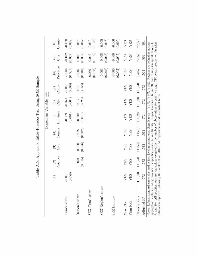
Tab

leA

.5:

App

endix

Tab

le–P

lace

bo

Tes

tU

sing

SO

ESam

ple

Dep

end

ent

Var

iab

le:

1µnit

(1)

(2)

(3)

(4)

(5)

(6)

(7)

(8)

(9)

(10)

Pro

vin

ceC

ity

Cou

nty

Pro

vin

ceC

ity

Cou

nty

Pro

vin

ceC

ity

Cou

nty

Fir

m’s

shar

e-0

.055

-0.0

39-0

.071

-0.0

66-0

.086

-0.1

02-0

.138

(0.0

59)

(0.0

61)

(0.0

64)

(0.0

80)

(0.0

61)

(0.0

67)

(0.0

89)

Reg

ion

’ssh

are

-0.0

210.

000

-0.0

27-0

.018

0.01

70.

011

-0.0

070.

010

0.04

5(0

.015

)(0

.026

)(0

.042

)(0

.016

)(0

.028

)(0

.058

)(0

.018

)(0

.032

)(0

.067

)

SE

Z*F

irm

’ssh

are

0.05

00.

049

0.04

9(0

.138

)(0

.139

)(0

.138

)

SE

Z*R

egio

n’s

shar

e-0

.003

-0.0

05-0

.005

(0.0

48)

(0.0

48)

(0.0

48)

SE

ZD

um

my

-0.0

00-0

.000

-0.0

00(0

.005

)(0

.005

)(0

.005

)

Yea

rF

Es

YE

SY

ES

YE

SY

ES

YE

SY

ES

YE

SY

ES

YE

SY

ES

Fir

mF

Es

YE

SY

ES

YE

SY

ES

YE

SY

ES

YE

SY

ES

YE

SY

ES

Ob

serv

atio

ns

1115

2011

1520

1115

2011

1520

1115

2011

1520

1115

2072

657

7265

772

657

Ad

just

edR

2.5

72.5

72.5

72.5

72.5

72.5

72.5

72.5

64.5

64.5

64

Note

s:R

obust

standard

erro

rscl

ust

ered

atfirm

leve

lin

pare

nth

eses

.Sig

nifi

cance

:∗∗

∗ :1%

,∗∗

:5%

,∗ :

10%

.R

egio

ns

are

defi

ned

atva

riou

sagg

rega

tion

leve

ls,

incl

udin

gpro

vin

ce(i

nsp

ecifi

cati

ons

2,

5,

and

8),

city

(in

spec

ifica

tions

3,6,

and

9),

and

county

(in

spec

ifica

tion

s4,

7,

and

10).

All

spec

ifica

tion

sar

ere

gres

sions

wei

ghte

dby

the

num

ber

ofobse

rvat

ions

for

each

two-d

igit

CIC

sect

orpro

duct

ion

funct

ion

esti

mat

ion

rep

orte

d(f

ollow

ing

De

Loec

ker

etal.

201

4).

All

regre

ssio

ns

incl

ude

aco

nst

ant

term

.

A. Proof of Proposition 1

Suppose marginal costs of all firms are bounded and non-decreasing. Proposi-tion 1 has the following five parts:

1) If operating independently, firm markups are increasing in a firm’s ownmarket share,

2) If operating as a cartel, cartel markups are increasing in total cartel marketshare with each firm’s own market share playing no additional role,

3) Firm markups are higher under cartel decisions than when operating inde-pendently,

4) Firm markups are more similar when operating as a cartel than when op-erating independently,

5) Firm market shares are more similar when operating independently thanwhen operating as a cartel

PROOF:Suppose any firm n in industry i weights the profits of the set of firms S ⊂ Ωi

with constant κ ∈ [0, 1]. Then their objective is:

(1) maxyni

p(yni)yni − C(yni;Xni) + κ∑m∈S

[p(ymi)ymi − C(ymi;Xmi)]

Then for µni defined as price divided by marginal cost and share defined as thefirm’s revenue divided by the sum of firm revenues in the industry, the firm’s firstorder condition can be rewritten as:

(2)1

µni= 1 + (1− κ)

∂ log(pni)

∂ log(yni)+ κ

∑m∈S

smisni

∂ log(pmi)

∂ log(yni)

If inverse demand is given by:

(3) pni = Diy−1/σni

∑m∈Ωi

y1−1/σmi

σγγ−1σ−1−1

Then the cross-price elasticities are:

(4)∂ log(pmi)

∂ log(yni)=

(1

σ− 1

γ

)sni

The own-price elasticity is:

(5)∂ log(pni)

∂ log(yni)= − 1

σ+

(1

σ− 1

γ

)sni

1

Together these imply that:

(6)1

µni= 1− 1

σ+

(1

σ− 1

γ

)((1− κ)sni + κ

∑m∈S

smi

)

Firms operating independently is the case where κ = 0, so then:

(7)1

µni= 1− 1

σ+

(1

σ− 1

γ

)sni

This implies result 1, when σ > γ. Likewise, if firms are operating as a perfectcartel, then κ = 1:

(8)1

µni= 1− 1

σ+

(1

σ− 1

γ

)∑m∈S

smi

This immediately implies the second result. Moreover, equations (7) and (8)together imply the fourth result, as cartels have no variation in markups (even ifthey have variation in market shares) while independent firms have markups thatvary with their shares.

To compare firms in a cartel to those operating independently, we construct anartificial single firm that is equivalent to the cartel. That is, suppose κ = 1 sothat the cartel solves:

(9) maxymi

∑m∈S

(pmiymi − C(ymi;Xmi))

where pmi is given by (3). Now define a cartel aggregate of production:

(10) Y =

(∑m∈S

y1−1/σmi

) σσ−1

Let C(Y ) be the cost function of the cartel defined as:

(11) C(Y ) = minymi

∑m∈S

C(ymi;Xmi)

subject to: Y =

(∑m∈S

y1−1/σmi

) σσ−1

2

Then the following problem is equivalent to (9):

(12) maxY

DiY1−1/σ

(Y 1−1/σ +

∑n/∈S

y1−1/σni

)σγγ−1σ−1−1

− C(Y )

First notice that the Envelope Theorem applied to the problem in (11):

(13) ∀m ∈ S, C ′(Y ) = λ =C ′(ymi;Xmi)

y−1/σmi Y 1/σ

Then we can relate the size of the cartel to the cost of the cartel’s production.

LEMMA 1: Consider a cartel made up of in T ⊂ S. Then for every level ofproduction Y , the marginal cost in the cartel composed of T is strictly higher thanin the cartel composed of S.

To prove this lemma, suppose yTmi is how much firm m produces when part of thecartel composed of T and ySmi is how much the same firm produces when part ofthe cartel composed of S. Then for any given Y it must be the case that:

ySmi < yTmi =⇒ C ′(ySmi;Xmi)

ySmi−1/σ

Y 1/σ<C ′(yTmi;Xmi)

yTmi−1/σ

Y 1/σ=⇒ CS

′(Y ) < CT

′(Y )

where the second implication follows from the fact that all firms have non-decreasing marginal costs. The first inequality follows from bounded marginalcosts and Inada conditions in the aggregation of individual firm production tocartel-level production. Therefore, if more firms are added to a cartel, marginalcosts for the cartel are reduced for every level of output.

Given this lemma, notice that as a cartel grows, the markup that the cartelcharges strictly increases. This follows immediately from that fact that, given thelemma, marginal costs decline so cartel production increases, and as another firmfrom within the same industry is brought into the cartel, that firm’s production isno longer counted in the denominator when computing the cartel’s market share.Therefore, the cartel’s market share strictly increases as more firms are added.Hence, by (8), the markup charged by the cartel increases.

A special case of this result is part 3 of Proposition 1. If a firm is operatingoutside of an existing cartel then is brought into it, the new cartel would havestrictly higher markups than either the original cartel or the formerly independentfirm.

To demonstrate the last result, consider any two firms n and m within the samecartel. Manipulating (13) gives:

(14)C ′(ymi;Xmi)

C ′(yni;Xni)=

(ymiyni

)− 1σ

=

(smisni

) 11−σ

3

Then consider two other firms v and w that are operating independently. Thenthe relationship between marginal cost and market share is:

(15)C ′(yvi;Xvi)

C ′(ywi;Xwi)=

(sviswi

) 11−σ 1− 1/σ + (1/σ − 1/γ)svi

1− 1/σ + (1/σ − 1/γ)swi

Suppose these two pairs of firms have the same relative marginal costs. Then:

(16)C ′(ymi;Xmi)

C ′(yni;Xni)=

C ′(yvi;Xvi)

C ′(ywi;Xwi)=⇒

(smisni

) 11−σ

=

(sviswi

) 11−σ 1− 1/σ + (1/σ − 1/γ)svi

1− 1/σ + (1/σ − 1/γ)swi

Without loss, if firms v and m have relatively high costs, then:

(17)C ′(ymi;Xmi)

C ′(yni;Xni)=

C ′(yvi;Xvi)

C ′(ywi;Xwi)> 1 =⇒

1− 1/σ + (1/σ − 1/γ)svi1− 1/σ + (1/σ − 1/γ)swi

> 1 =⇒ snismi

>swisvi

Therefore, independently operating firms have wider variation in market sharesconditional on marginal cost than do firms operating as a cartel. This completesthe proof.

B. Simulation of Model with Shocks to Demand and Costs

We now consider a version of the model where some uncertainty in costs ordemand is realized after production choices are made. Firm i in industry j locatedin region k in year t solves the following problem:

maxlijkt

∫Sε

∫Sρ

(1− κ)πijkt(l, ε, ρ) + κ∑

m∈ωjkt

πmjkt(l, ε, ρ)

dF (ε)dG(ρ)

where:

πijkt(l, ε, ρ) = Dj(εijktl1/ηijkt)

1−1/σ

∑m∈Ωjt

(εmjktl1/ηmjkt)

1−1/σ

σγγ−1σ−1−1

− ρijktlijktzijkt

Here ε is the vector of demand shocks, ρ is the vector of cost shocks, and l is thevector of production choices. The set of firms operating in industry j at time t isΩjt, and its subset of firms operating within region k is ωjkt. For any given firm,zijkt is the component of their costs that is known before production decisions

4

are made. Without heterogeneity in this, there would be no heterogeneity in lijkt.The parameter η allows for curvature in the cost function.

Notice that F and G are probability distributions over vectors, and we willconsider covariance at the cluster, industry and year levels.

The first order condition implies:∫Sρ

ηρijktl1−1/η

ijkt

zijktdG(ρ) =

=

∫Sε

pijkt(l, ε)

σ − 1

σ+

(1

σ− 1

γ

) κ(εijktl1/ηijkt)

1−1/σ + (1− κ)∑

n∈ωjkt

(εnjktl1/ηnjkt)

1−1/σ

∑m∈Ωjt

(εmjktl1/ηmjkt)

1−1/σ

dF (ε)

where:

pijkt(l, ε) = Djε1−1/σijkt l

−1/ησijkt

∑m∈Ωjt

(εmjktlmjkt)1/η(1−1/σ)

σγγ−1σ−1−1

Firms face a variety of shocks at different levels:

εijkt = ν1ε1t + ν2ε

2jt + ν3ε

3ijkt + ν4ε

4jkt + ν5ε

5kt

ρijkt = µ1ρ1t + µ2ρ

2jt + µ3ρ

3ijkt + µ4ρ

4jkt + µ5ρ

5kt

Therefore, we can separately analyze shocks at different levels.

Computational Implementation

The simulated dataset has T years, J industries and K regions. Every industry-region-year has I firms within it. The vectors ε and ρ are therefore of lengthI × J × K × T . First, both ε and ρ are simulated M times. Then a vector Lis drawn. Then L is input as the vector of production choices of firms. Usingthe first order condition, we then solve for the vector Z of anticipated costs thatrationalizes the vector L. Together, Z, L, and the realization of shocks impliesmarkups (using the method of De Loecker and Warzynski) and market shares foreach firm. Then, for each realization, the regression described in the paper is runon the simulated data. This is done M times.

For these results we choose σ = 11, γ = 3, and κ = 0.3. We set T = 5, J = 5,K = 8, I = 5 and M = 2000. We assume that all the log of each shock is astandard normal random variable.

5

Effects of Shocks on Estimation of κ

First we look at the effects of all twelve types of shocks individually. The tablebelow presents the results of setting µ1 = ... = µ5 = ν1 = ... = ν5 = 0, thenindividually setting each to 1.

In each iteration of the simulation we run the following regression:

1

markupijkt= α+ β1sijkt + β2cjkt + δijkt

where:

sijkt =(εijktyijkt)

1−1/σ∑m∈Ωjt

(εmjktymjkt)1−1/σ

cjkt =∑l∈ωjkt

sljkt

Here we present the simulated moments of κ defined by:

κ ≡ β2

β1 + β2

No Fixed Effects Region-Year and Firm FEs

Cost Shocks: Avg. κ St. Dev. κ Avg. R2 Avg. κ St. Dev. κ Avg. R2

Year 0.3000 0.0386 < 10−4 0.2985 0.0385 0.6656Industry-Year 0.2990 0.0322 < 10−4 0.2994 0.0383 < 10−4

Firm-Year -2.6347 12.3521 0.0020 0.1248 6.1992 0.0024Cluster-Year 0.7824 2.3801 0.0051 0.9452 0.4269 0.0071Region-Year 0.9820 1.0814 0.0063 0.2998 0.0460 0.4797

Demand Shocks: Avg. κ St. Dev. κ Avg. R2 Avg. κ St. Dev. κ Avg. R2

Year 0.2985 0.0147 < 10−4 0.2953 0.0265 0.7591Industry-Year 0.3015 0.0230 < 10−4 0.2986 0.0287 < 10−4

Firm-Year -0.0007 0.0381 0.1551 0.0057 0.0505 0.1560Cluster-Year 0.9815 0.0028 0.2953 0.9822 0.0036 0.2892Region-Year 0.9805 0.0055 0.3553 0.6792 0.0830 0.0496

6

Firm FEs Region-Year FEs

Cost Shocks: Avg. κ St. Dev. κ Avg. R2 Avg. κ St. Dev. κ Avg. R2

Year 0.2984 0.0095 < 10−4 0.3008 0.0173 0.5853Industry-Year 0.2915 0.0615 < 10−4 0.2987 0.0489 < 10−4

Firm-Year -0.7124 4.7541 0.0024 -3.4905 51.4933 0.0020Cluster-Year 0.9273 1.9951 0.0051 1.0789 0.6426 0.0062Region-Year 0.9822 0.2574 0.0052 0.2958 0.0570 0.3867

Demand Shocks: Avg. κ St. Dev. κ Avg. R2 Avg. κ St. Dev. κ Avg. R2

Year 0.3009 0.0320 0.0001 0.2999 0.0253 0.7812Industry-Year 0.2994 0.0265 < 10−4 0.2983 0.0334 < 10−4

Firm-Year 0.0021 0.0482 0.1029 -0.0014 0.0574 0.1220Cluster-Year 0.9826 0.0038 0.1894 0.9811 0.0036 0.2227Region-Year 0.9805 0.0069 0.2193 0.6892 0.0678 0.0507

7