GROWTH FOLLOWING INVESTMENT AND CONSUMPTION-DRIVEN CURRENT ACCOUNT CRISES · GROWTH FOLLOWING INVESTMENT AND CONSUMPTION-DRIVEN CURRENT ACCOUNT CRISES Alexander Klemm* Current account

GROWTH FOLLOWING INVESTMENT AND CONSUMPTION-DRIVEN CURRENT ACCOUNT CRISES

Alexander Klemm*

Current account deficits imply increasing liabilities to the rest of the world. External sustainability then depends on whether these can be met in the future without defaulting, i.e., normally through trade account surpluses. To run such surpluses without a fall in consumption, capital inflows should be used to increase future output. This paper tentatively finds that current account deficits reversals that follow investment booms are marked by better growth performance than those following consumption booms. It also shows that many recent large current account deficits have been predominantly the result of consumption or non-productive investment booms.

1 Introduction

The current sovereign debt crisis in Europe has brought not only budgetary discipline back to the fore, but more generally economic imbalances. Indeed, looking at euro area fiscal and current account deficits prior to the crisis (Table 1), it appears that measures of external balances have been better at identifying countries that would run into difficulties.

By definition the current account balance is equal to the difference between savings and investment. However, a given savings shortfall can be the result of very different absolute amounts of savings and investment. While this is obvious, this paper argues that this may merit more attention than it has been given in the past, and that it may be relevant for the assessment of external sustainability.1

Running a current account deficit implies that liabilities to the rest of the world are increasing. To assess external sustainability, it is therefore necessary to ascertain whether these liabilities can be met in the future without defaulting, i.e., normally through running future trade account surpluses. To run future trade account surpluses without a fall in consumption, the economy will have to use the capital inflow that occurs to increase future output. This can be achieved for example by increasing the rate of investment in assets that produce future returns, which can be used to pay off the creditors. In other words, the economy’s capacity for producing tradable goods and services needs to increase.

One exception to this mechanism is the possibility that liabilities can be reduced through valuation effects.2 E.g., a devaluation or depreciation will increase the value of foreign assets relative to liabilities as long as liabilities are denominated in domestic currency. It is also possible that rates of return on foreign assets exceed those of domestic assets held by foreigners, which would reduce the value of net liabilities. Some commentators have argued that this was the case in the USA (e.g., Kitchen (2007)), although it remains controversial, as the data are incomplete (Gros, 2006). The scope for valuation effects clearly depends on the structure of assets and liabilities, e.g., foreign-currency denominated debt is unlikely to be reduced significantly through valuation effects,

————— 1 Higgins and Klitgaard (2011) is one of a few papers that mention this idea. 2 And, as argued in Nickell (2006), these effects could be huge in some countries, such as the UK, where the current account deficit is

small compared to the stock of international assets and liabilities.

2 Alexander Klemm

Table 1

Euro Area Countries’ Pre-crisis Balances, 2007 (percent of GDP)

Fiscal Balance

Greece –6.5

Portugal –3.1

France –2.7

Malta –2.3

Slovakia –1.8

Italy –1.6

Austria –0.9

Belgium –0.1

Slovenia 0.0

Ireland 0.1

Germany (until 1990 former territory of the FRG)

0.2

Netherlands 0.2

Spain 1.9

Cyprus 3.5

Luxembourg 3.7

Finland 5.3

Source: Eurostat. Countries that required a support program printed against grey background.

while the liabilities connected to non-debt creating FDI could be reduced to nil if the investment turns out unsuccessful.

Theoretically, the starting point for a study of balance of payments pressure would be the net international investment position, which should be the result of past current account balances and valuation effects. A negative position would indicate the need for adjustment through future current account surpluses and/or devaluation. However, the quality of data on the international investment position is very questionable, as valuation effects are difficult to estimate. Gros (2006), for example, shows that for the US the discrepancy between cumulated current account deficits over 1985-2005 and the change in net international investment decisions amounted to an impressive $2.6 trillion, which he argues cannot be explained even when taking valuation effects into account. We therefore look at cumulative current account deficits instead, but will need to remember that liabilities to the rest of the world need not be completely fulfilled through future current account surpluses.

Current Account Balance

Greece –14.6

Cyprus –11.7

Portugal –10.1

Spain –10.0

Malta –6.2

Ireland –5.3

Slovakia –5.3

Slovenia –4.8

Italy –1.3

France –1.0

Belgium 1.9

Austria 3.5

Finland 4.3

Netherlands 6.7

Germany (until 1990 former territory of the FRG)

7.4

Luxembourg 10.1

Growth Following Investment and Consumption-driven Current Account Crises 3

While a current account deficit necessarily implies capital imports, it does not necessarily increase domestic investment.3 Instead, the local savings rate could decrease, so that consumption would rise with investment staying flat. More precisely, when a country runs a current account deficit, this could have the following consequences (or combinations thereof):

1) Additional capital is imported so that the economy’s capital stock increases.

2) Capital owned by residents is sold to non-residents, with no change in the stock of capital located in the economy.

a) Residents reduce their net holdings of productive capital (possibly to below zero by issuing debt) and consume the proceeds.

b) Residents sell capital to foreigners and the foreign demand bids up prices. Residents therefore maintain their financial capital, but own a smaller share of real capital.

The implication on liabilities is different, each time. Under 1, there is a foreign liability, but also a domestic asset producing returns. Theoretically, this would also include certain investment in human capital such as the financing of scholarships abroad, provided students return and use their skills for tradable production. A future reversal in the current account could then in principle occur without any crisis, simply as a result of the investment facilitating the production of tradables. A particularly obvious case is the investment in mining equipment, which may then lead to current account surpluses as soon as natural resources are mined and exported.

Under 2a there is the same foreign liability, but no domestic asset, hence future consumption must be reduced to service the liability. Under 2b domestic investors own less of the economy’s real capital, but they may not notice it, because of the value of financial capital may be the same as before. If the asset price bubble bursts, resident investors will notice it and reduce their consumption. However, not as much as under 2a, as the value of domestic assets held by foreigners declines also.

There are countless other possibilities and combinations thereof. But these illustrations certainly show that domestic investment may not increase as a result of capital imports, not even when the value of domestic assets increases. The role of the real domestic capital stock may therefore be important and will be examined more closely in the empirical part.

Many different, but equivalent, processes may take place behind these possibilities. The first possibility, for example, could be directly the result of foreign investors buying foreign investment goods and bringing them into a country. Equivalently, it could also be the result of domestic producers switching production from consumption goods to domestically-sold investment goods, while total consumption is maintained through imported consumption goods financed by loans from foreign banks. In both cases, productive capacity is enhanced and as long as the investment turns out successful, it will allow closing the current account deficit in the future without a drop in consumption. It is therefore not relevant whether imports are in consumption or investment goods, nor whether the rest of the world acquires domestic debt or physical assets (at least for this purpose), but whether the capital stock increases compared to the case in which the current account were balanced.

The different investment levels behind current account deficits are likely to have important implications for sustainability. In the first case, the future trade account surpluses that are required can be supplied by the additional capital, and domestic consumption does not need to be reduced. In the second case, domestic consumption is higher now, but will be permanently lower than it

————— 3 Some confusion may arise from the different meanings of the term capital. Capital, in the sense of foreign funds is typically

imported to finance a current account deficit. But that does not mean that capital, in the sense of a physical or human capital stock is build up.

4 Alexander Klemm

would have been without the initial current account deficit. In case 2b this may be less obvious to residents than in case 2a, as they will initially not notice a decrease in their wealth.

An impact of investment on the current account would have implications for public policy. Apart from the well-known channel of the public sector deficit affecting the current account, there could be another channel through public investment, so that for a given public sector deficit, current account outcomes may be more or less sustainable, depending on public investment relative to consumption expenditure, and the quality of the public investment. Moreover, the impact hinges on whether public and private investments are substitutes or complements.

There is a related, but different literature looking more directly at the link between the fiscal and current account deficits. Funke and Nickel (2006) point out that the empirical literature has tended to find ambiguous results on this link. Their own analysis is also ambiguous, which they explain by the counter-acting effects of public spending on aggregate demand and crowding out of private spending. IMF (2011), however, argues that fiscal policy does have a strong impact on current account deficits. They base this finding on results from an action-based fiscal variable data set, which they argue is reliably exogenous. In any case, none of these studies distinguish between public consumption and investment.

Another related literature has looked at the sustainability of current account balances. One theory was that current account deficits were necessarily sustainable if the result of private-sector behavior (“Lawson doctrine”), but this does not stand up to empirical evidence as shown by Reisen (1998). There are also various studies of particular countries, especially the US, where views on the sustainability of the current account deficit and the process and implications of its reduction differ widely.4

One further possible approach to this question is the intertemporal view of the current account (surveyed by Obstfeld and Rogoff, 1995). Under this view, the sustainability of the current account depends on future developments of incomes and expectations thereof. A current account deficit could, for example, be the result of an expected future income boom. Such a deficit would then not imply an unsustainable consumption path, even if it is the result of an increase in consumption rather than investment. In most cases, however, an intertemporal interpretation of the current account would not come to different conclusions than the illustration above. Except in the case of a natural resource find, which would immediately make a country richer, it is likely that any future increase in income is related to an increase in the domestic capital stock, although other factors, such as demographic developments and structural reforms (which in turn may also boost investment) will also play a role. Hence a sustainable deficit is likely to be accompanied by high real investment rates. And if a country believes that it will get rich without more capital (e.g., simply by joining the EU), then it is quite likely to be proved wrong at a later point, and the current account deficit will have been unsustainable, even though it appeared sustainable based on wrong expectations. Moreover, as argued in Reisen (1998), it is hard to establish any clear benchmarks for excessive current account deficits using the intertemporal approach.

The paper most closely related to this one is Milesi-Ferretti and Razin (1998) which looks empirically at the consequences of current account reversals. While that paper does not cast this as a question of consumption versus investment-related current account deficits, it adds the investment share of GDP as an explanatory variable and finds that a high share leads to higher post-reversal growth. A less directly related paper is Milesi-Ferretti and Razin (2000) which, among other things, looks at determinants of current account reversals and finds that high ————— 4 E.g., Papers arguing in favor of sustainability include Hausman and Sturzenegger (2006) who note the relatively strong position of

net liabilities. Papers arguing against include Edwards (2005) and Gros (2006) who questions the quality of data on liabilities. Some papers are undecided and note that it depends on assumptions about future developments of variables, particularly US relative to world income, e.g., Engel and Rogers (2006).


Table 2

Descriptive Statistics

Variable Unit Obs. Mean Min. Lower

QuartileMedian

Upper Quartile

Max.

Current account % of GDP 5,217 –3.6 –240.5 –7.5 –3.1 0.7 56.7

Investment % of GDP 7,494 23.2 –17.4 18.3 22.4 26.9 113.6

Fixed inv. % of GDP 7,209 22.2 1.9 17.8 21.5 25.4 113.6

Gov. fixed inv. % of GDP 3,604 7.4 –3.4 4.0 6.4 9.3 43.0

Private fixed inv. % of GDP 3,608 14.3 –2.6 9.7 13.8 17.9 112.4

Real growth % change 8,247 3.7 –51.0 1.5 3.8 6.1 106.3

Real effective exchange rate % change 2,593 0.7 –100.0 –7.4 0.0 6.4 1,415.6

Terms of trade % change 4,057 2.1 –80.9 –5.8 0.0 6.4 1,213.3

Openness (exports+imports) % of GDP 7,726 77.4 0.3 44.9 66.3 100.1 460.5

GNI per capita US$ 7,790 6,620 60 550 1,830 6,550 185,730

Source: Author’s calculations based on World Development Indicators, except terms of trade: World Economic Outlook.

investment share increases the likelihood of a reversal. This reversal could occur through two rather different channels, either with the investment leading to increased production of tradable goods or with imbalances making countries vulnerable to sudden stops.

To sum up the introductory thoughts – while it is obvious that current account deficits can be due to savings shortfalls as well as consumption booms – so far little attention has been paid to the relationship between external deficits and real domestic investment or, in stock terms, external liabilities and the real domestic capital stock and their implications for current account reversals. Still, the likelihood of a reversal and its implications for domestic savings may strongly depend on how foreign capital imports are used. This paper attempts to fill this gap looking empirically into these issues and drawing from the various related literatures.

The rest of this paper is structured as follows: Section 2 provides a descriptive analysis using table and charts that show the underlying developments behind recent current account imbalances. Section 3 provides an econometric analysis of the impact of investment on economic conditions following a current account reversal. Section 4 concludes.

2 Descriptive analysis

2.1 Data

The data are from the World Bank’s World Development Indicators (December 2012 update) except data on the terms of trade which are from the IMF’s World Economic Outlook (October 2012). From these data we keep only observations from 1970 to 2011. Disregarding observations where basic variables such as GDP are missing the sample covers 204 economies. Some descriptive statistics are provided in Table 2.

6 Alexander Klemm

2.2 Methodology and findings

Many existing descriptive analyses depict current account deficits, savings and investment over time. A recent example is Higgins and Klitgaard (2011) who use such charts to show that in European periphery countries, current account deficits were mainly the result of low savings rates in Greece and Portugal, while financing a housing boom in Spain and Ireland. Instead of following this approach, this paper will look at country-specific episodes of current account imbalances and the cumulative savings and investments related to them.

We start with very basic macroeconomic accounting, with GDP as the sum of consumption (C), investment (I) and net exports (X). Instead of adding a term for government spending, we split consumption and investment separately into private (IP, CP) and public (IG, CG), but only when needed.

(1)

Gross National Income (GNI) consists of GDP and net income from abroad (YF). It can be consumed or saved (S).

(2)

Putting this together yields the usual result that the current account (CA) is equal to savings less investment.5

(3)

When looking at the government sector, some confusion can arise because of inconsistent terminologies. Sometimes the budget balance is called “public saving”, but here we will use this term only for the budget balance net of investment spending, which is more in line with the definition of private savings.

To study current account imbalances, the analysis starts in times of balanced current accounts, which we define as years in which current account surpluses or deficits remain below 1 per cent of GDP. When a current account imbalance starts evolving we will look at the cumulative implications. For ease of exposition let us rewrite the current account formula from above:

(4)

Then we consider the change in the current account to GDP ratio compared to the last year without a current account imbalance, which is approximately equal to the change in the ratios of consumption and investment to GDP:

(5)

To reduce the problem of double-counting of current account episodes, we define current account events. These are years in which the current account deficit peaks over a 10-year horizon,6 provided it reaches at least 5 per cent of GDP. There are 252 such events in our dataset, and 129 out of the 204 countries have at least one. A complete list of all such events is given in Table 8 in

————— 5 Note that some textbooks do not distinguish carefully between GNI and GDP and hence between the current account deficit and net

exports. 6 To avoid artificial deficit peaks at the beginning and end of sample, we exclude the first and last three years per country as

candidates for peaks. A peak is therefore defined as an observation where the current account deficit exceeds the one of the preceding 3 years and the following 6 years, or the preceding 4 year and following 5 years, or preceding 5 years and the following 4 years, or preceding 6 years and the following 3 years.

)( XICICXICY GGPP ++++=++=

SCYY F +=+

CAYXIS F =+=−

ICYYISCA F −−+=−=

Y

I

Y

C

Y

I

Y

C

Y

Y

Y

CA F

Δ−Δ−≈Δ−Δ−Δ=Δ


Table 3

Increases of Consumption and Investment Shares in Current Account Deficit Peaks (percent of GDP)

Consumption Investment

Total Private Public Total Fixed Private Fixed Public Fixed

Obs. 233 230 228 233 226 116 116

Mean 4.8 3.5 1.2 4.1 3.9 4.6 0.8

Median 3.5 2.3 0.7 3.7 3.5 3.7 0.4

Source: Author’s calculation based on World Development Indicators.

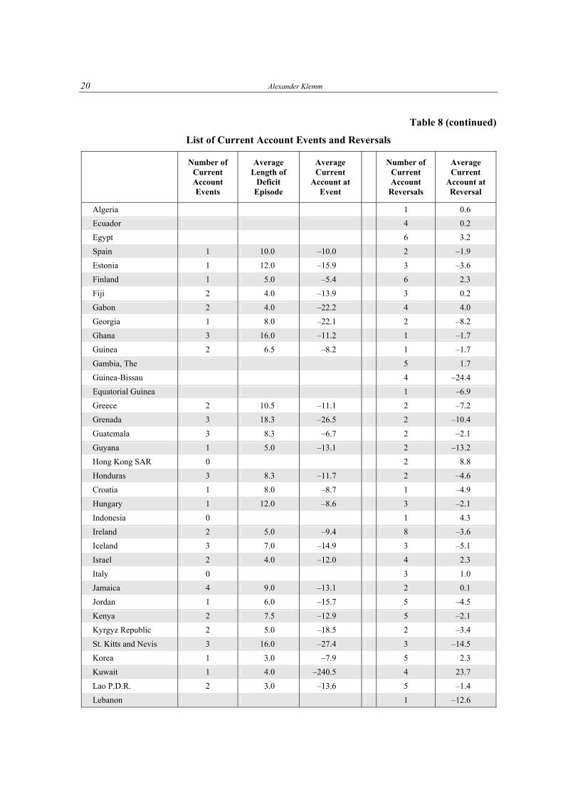
the Appendix. For most of these events we have also data on consumption and investment; and in some cases also a breakdown of private and public fixed investment.

As shown in Table 3, on average, more than half of the increase in current account deficits was associated with more consumption (or reduced saving), which rose 4.8 percentage points of GDP compared to 4.1 percentage point increase in investment. This already confirms that in practice, current account deficits are to an important extent associated with an increase in consumption rather than saving. Moreover, on average these developments were dominated by private sector flows, which were responsible for most of the increase in consumption and virtually all of the increase in investment.

As these averages hide differences in country-specific developments, the next step is to look at developments in individual countries. This is done with the help of charts, which show the current account deficit and the cumulative increase in investment and consumption shares in GDP since the start of the current account imbalance.

Figure 1 presents developments in large economies, showing the USA and the UK as examples for countries with large current account deficits, and Germany and Japan as examples of large surpluses.

• For the US, the chart shows that current account deficits of the 1980s started with increases in investment, followed by a disappearance of the deficit and less investment. The current account deficit, which began appearing in the early 1990s, was also initially marked by an increase in investment. Since the early 2000s, however, consumption has also grown heavily, and in the late 2000s the investment share actually fell below the level seen before the start of the deficit.

• In the UK, the deficit in the 1980s was similarly marked by an increase and subsequent fall in investment, although a smaller deficit in the early 1990s was marked by consumption growth. The latest deficit episode, however, which started in 1999, has been marked since the beginning by a rising share in consumption; recently this has turned so strong that a current account deficit remained despite a fall in the investment share.

• In Germany, large surpluses in the 1980s were marked by high saving, while the investment share remained relatively constant. The even larger surpluses of the 2000s, however, were marked by both savings and reductions in investment.

• In Japan, the situation is different in that the current account surplus has been the most stable feature of the economy, while the role of savings and investment changed over time. Most remarkably, the consumption share of GDP grew much more than in the US and the UK, but a simultaneous reduction in domestic investment meant that the current account surplus was maintained.

8

Alexander K

lemm

Figure 1

Current Account Developments in Selected Large Economies

Source: Author’s calculation based on WDI data.

USA UK

Germany Japan

1970 1980 1990 2000 2010 1970 1980 1990 2000 2010

1970 1980 1990 2000 2010

1970 1980 1990 2000 2010

0.06

0.04

0.02

0

–0.02

0.02

0

–0.02

–0.04

–0.06

–0.08

0.05

0

–0.05

0.1

0.05

0

–0.05

–0.1

Current account deficit Add. Inv. Add. Cons.


Figure 2 shows developments in euro area crisis and vulnerable countries.

• In Greece, the current account deficit episode was originally marked by rising investment shares, but since the mid-2000s investment started falling.

• In Portugal, a similar pattern applies, with deficits being first associated with high investment and then consumption.

• In Ireland past current account deficits were associated with rising investment shares. The most recent deficit also started with rising investment shares, but then investment fell strongly while consumption rose. By 2010, investment has fallen so much as to eliminate the deficit.

• In Spain, investment is strongly aligned with current account deficits, while consumption remains relatively stable.

Figure 3 provides a further breakdown of Spanish investment, as Spain is a well-known case of a housing investment boom, and as it is one of the few countries for which a more detailed investment breakdown can be obtained from WEO, at least for the most recent years. The figure confirms that most of the continued increase in investment was due to rising investment in residential structures, while investment in plant and machinery only rose in the beginning and then stayed flat until the onset of the crisis, when it collapsed. A small share of the investment in the housing stock may still contribute to future export earnings, as some houses were bought by foreigners who will keep spending on services when they visit as tourists or pensioners.

Figure 4 shows, for comparison, developments in selected previous crisis countries. These also show greater divergence, from consumption-related current account deficits in Argentina (1980s) and Brazil, to investment-related ones in Argentina (1990s), Thailand and Latvia.

To sum up this section we can note that in practice, current account deficits have often been associated with increased consumption (reduced saving) rather than increased investment. Worryingly, the large current account deficits in some advanced economies have recently been marked more by reduced savings than additional investment. This means that if they are reduced in the future, this will require a fall in the consumption share and not simply a reduction in investment from exceptionally high levels.

Even if current accounts are marked by increased investment, economies can end up in crisis, and indeed many historic crises were preceded by investment booms. There are many ways in which investment may not guarantee future current account surpluses, including cases where investment takes place in the non-tradable sector or where it is simply inefficient. But while an increase in investment may not guarantee a soft landing for large current account deficits, it is even harder to see such a solution for a deficit related to consumption booms – unless the present consumption boom is related to a foreseen (and actually occurring) future increase in incomes.

3 Econometric analysis

Having established that current account deficits are in practice both the result of consumption and investment booms, this section looks at the empirical implications for growth.

Obtaining robust empirical findings is quite challenging, given that current accounts and other imbalances can persist for a long time before adjustment takes place. A standard regression involving yearly data would be dominated by the many years in which imbalances are built up rather than when adjustment suddenly takes place. In order to focus on times following a current account adjustment, we look at developments around these periods. We use both the definition of a current account event (deficit peak) as described above, and one based on current account reversals proposed by Milesi-Ferretti and Razin (1998). Restricting the sample to these special cases of

10

Alexander K

lemm

Figure 2

Current Account Developments in Euro Area Crisis and Vulnerable Countries


Greece Portugal

Spain

0.15

0.1

0.05

0

–0.05

0.2

0.1

0

–0.1

–0.2

0.15

0.1

0.05

0

–0.05

–0.1

0.1

0.05

0

–0.05

1970 1980 1990 2000 2010 1970 1980 1990 2000 2010

Ireland

1970 1980 1990 2000 2010

1970 1980 1990 2000 2010

Current account deficit Add. Inv. Add. Cons.


Figure 3

The Composition of Additional Investment in Spain Source: Author’s calculation based on WEO data.

current account deficit peaks/reversals helps us in identifying the impact of investment shares in current accounts. Still, the more general result from the growth literature that investment is typically growth enhancing will also affects these results and cannot be separated econometrically. For a policy maker, the more relevant finding will be the impact of investment on post-current account reversal growth, irrespective of the precise channel through which it operates.

3.1 Results based on the contribution of investment to current account deficit peaks

Our first approach is closely linked to the graphical analysis above and relates growth performance following a current account adjustment to the level of the current account and the contribution of investment to that level:

(6)

where g is the growth rate – either of consumption or real GDP –, y captures time effects and ε is the error term and the other variables are changes in ratios since the beginning of an imbalance as defined above. The bar indicates that the growth rate is calculated over three-years: the three years following a current account deficit peak for the explained variable, and the three years preceding a peak in case of the explanatory variable. As the regression is estimated only for current account events (as defined above) we usually have only one or two observations per country and country fixed effects are not included.

εβββ ++Δ+Δ+= − tt yY

I

Y

CAgg 2110

0

0.02

0.04

0.06

0.08

0.1

1995 2000 2005 2010

Add. inv.

Add. residential struct.

Add. machinery/equipment

12

Alexander K

lemm

Figure 4

Current Account Developments in Selected Previous Crisis Countries


Current account deficit Add. Inv. Add. Cons.1970 1980 1990 2000 2010

1970 1980 1990 2000 2010

1970 1980 1990 2000 2010 1970 1980 1990 2000 2010

Latvia Argentina

Thailand Brazil

0.4

0.2

0

–0.2

–0.4

0.05

0

–0.05

0.1

0.05

0

–0.05

–0.1

–0.15

0.2

0.1

0

–0.1

–0.2


Table 4

Real Consumption Growth Following a Current Account Deficit Peak

(1) (2) (3) (4) (5)

0.109 0.097 0.097 0.165 0.022 Lagged real cons. growth

(0.124) (0.124) (0.121) (0.140) (0.185)

0.084 0.055 0.096 0.073 0.031 Δ Current account

(0.063) (0.066) (0.064) (0.083) (0.116)

0.148** 0.105* Δ Investment

(0.073) (0.054)

0.171** Δ Fixed Investment

(0.067)

0.063 0.054 Δ government fixed investment (0.168) (0.148)

0.257** 0.097 Δ private fixed investment

(0.104) (0.092)

Year effects yes yes yes

Observations 149 149 145 74 74

R2 0.0691 0.354 0.383 0.179 0.649

Adj. R2 0.0499 0.169 0.199 0.132 0.390

Dependent variable: Real consumption growth in the 3 years following an event. Explanatory variables: Lagged real cons. growth: calculated over the 3 years preceeding an event; Δ Current account, Δ Investment (total, fixed, government, private): change in GDP share from beginning of a current account episode. Robust standard errors in parentheses. *** p<0.01, ** p<0.05, * p<0.1

Before turning to overall growth, we consider the impact of the current account and its

components on consumption growth. As argued above, we expect consumption growth following a current account deficit peak to be stronger if the current account was associated with strong investment rather than low savings.

Results are shown in Table 4. The first two regressions consider the impact of total investment. They confirm that following a current account deficit peak, consumption growth is higher the greater the increase in the investment share prior to the peak. This is robust to the inclusion of year effects, which control for worldwide economic conditions. The coefficient of the change in the current account deficit has the expected sign, as a stronger current account is followed by higher growth, but is not statistically significant in this and most other specification. Regression (3) replaces total by fixed investment, which yields an even stronger positive impact on post-peak real consumption growth. Regressions (4) and (5) split fixed investment into a government and a private share. The result is that only private investment has a significant impact on real consumption growth, which could indicate that public investment is more likely to be

14 Alexander Klemm

Table 5

Real Growth Following a Current Account Deficit Peak

3-year Real Growth Least Dummy:

Squares with Robust S.E. 3-year Real Growth < 2.5% Probit Dep. Variable

Estimation (1) (2) (3) (4) (5) (6) (7)

0.229** 0.252** 0.231** Lagged real growth

(0.101) (0.109) (0.108)

0.010 0.005 0.008 0.061 0.244 –0.064 0.174 Δ current account

(0.009) (0.010) (0.010) (0.631) (0.789) (0.616) (0.745)

0.048 0.029 –1.675* –2.440* Δ Investment

(0.045) (0.032) (0.992) (1.328)

0.059 –1.894* –2.432* Δ Fixed Investment

(0.036) (1.071) (1.402)

Year effects yes yes yes yes

Observations 149 149 145 229 221 222 212

R2 0.0691 0.354 0.383

Adj. R2 0.0499 0.169 0.199

Explanatory variables: Lagged real cons. growth: calculated over the 3 years preceeding an event; Δ Current account, Δ Investment (total, fixed, government, private): change in GDP share from beginning of a current account episode. Standard errors in parentheses. *** p<0.01, ** p<0.05, * p<0.1

wasted or otherwise not contributing to enhancing the productive capacity. The result, however, does not survive the inclusion of year effects, which may be partly due to the reduced sample size.

Next we consider total economic growth. There a positive impact of investment may still be expected, but it could be less strong, because a collapse of investment may also have a negative impact in the short term, unless all investment goods were imported or the economy is very flexible. Results are shown in Table 5.

The first three regressions mirror the ones on consumption growth. However, now the lagged dependent variable turns significant, while the investment variables are not significant anymore – although for fixed investment (regression (3)) the p-value at 10.4 is close to standard thresholds for significance. Regressions (4)-(7) look at the probability of growth being low (i.e., below 2.5 per cent over three years, which is just below the median) for total and fixed investment with and without year effects. For these less demanding specifications, there is evidence that the risk of very low growth is reduced when current accounts are associated with investment booms.

3.2 Results based on the current account reversals as developed by Milesi-Ferretti and Razin (1998)

In addition to specifications closely related to the descriptive part, we also employ an approach developed by Milesi-Ferretti and Razin (1998). They look at three year averages before


and after current account reversals. Closely following their approach, a reversal is then defined as a reduction in the average current account deficit to GDP ratio over 3 years by at least 3 percentage points over the preceding years. Additionally the deficit must be reduced by at least a third and the highest post-reversal deficit must be below the lowest pre-reversal deficit. On the dataset made up by reversals only, the following regression is run:

(7)

where x is a vector of control variables and all other variables are defined as before. The bar over CA and I indicates that the three-year pre-reversal average is taken. One minor difference compared to Milesi-Ferretti and Razin (1998) is that we use a year dummy instead of calculation deviations from world averages.

On control variables we also closely follow Milesi-Ferretti and Razin (1998), although we skip the interest rates (which were hardly ever significant in their paper). Our precise definitions are:

• Real effective exchange rate (REER) appreciation: this is appreciation over the three years before the reversal and is a measure of the change in competitiveness of the economy.

• Change in terms of trade: this is change in the terms of comparing the three years before and after the event. This is to control for the effect of changes in world prices (e.g., commodity prices) on the current account.

• Openness: this is the pre-reversal share of exports and imports in GDP, which may affect the likelihood of a current account reversal, as well as its size and impact.

• GNI per capita: this is a measure of the pre-reversal income of the economy, to control for convergence, i.e., higher growth rates in poorer economies.

Results are shown in Table 6. Regression (1) is the simplest implementation with no controls. It is therefore directly comparable to the previous regression, just that the data set is larger because of the different definition of a current account event, and that we use three year averages of explanatory variables instead of the previous cumulative change in ratio since the beginning of a current account episode. Also in this specification, there is a positive and significant impact of investment on growth, controlling for its impact on the current account. Regression (2) adds the control variables and the results now show an even stronger impact of investment. Moreover, they are similar to those reported in Milesi-Ferretti and Razin (1998), except that in their results the lagged real growth rate is not significant, while the openness indicator is. Most of the control variables are widely available, but the REER reduces the sample size a lot. Removing this variable increases the sample size, but does not affect the coefficient on investment much. Replacing total investment by fixed investment in Regression (4) leads to even stronger results (also in specifications without controls or with the REER, which are not shown). Regression (5) considers public and private fixed investment separately and finds similar coefficients on both, although only the one on private investment is statistically significant.

3.3 Robustness checks

Given that the interest of this paper has been to study current account imbalances, most of the observations used in regressions relate to the most extreme outcomes occurring in the sample. Removing outliers therefore has different implications in such an exercise as in a normal one. Hence, when dropping only the top and bottom five percentiles of the distribution of the current account and investment ratios as well real growth, the sample of current account deficit peaks (or reversals) is reduced significantly. Still, while the results generally got weaker, they held up,

εββββ +++++= −−−

− tttt

t yxY

I

Y

CAgg '1

12

1110

16 Alexander Klemm

Table 6

Real Growth Following a Current Account Reversal

(1) (2) (3) (4) (5)

0.219* 0.232*** 0.173 0.175 0.124 Lagged real growth

(0.115) (0.079) (0.137) (0.136) (0.162)

0.027 0.070** 0.032 0.035 0.049 Current account/GDP

(0.026) (0.034) (0.029) (0.028) (0.041)

0.054* 0.078* 0.092** Investment/GDP

(0.032) (0.040) (0.043)

0.098** Fixed investment/GDP

(0.043)

0.105 Public investment/GDP

(0.064)

0.107* Private investment/GDP

(0.059)

–0.077* REER

(0.040)

0.011 0.036*** 0.037*** 0.053*** Δ terms of trade

(0.013) (0.012) (0.012) (0.015)

0.002 0.001 0.001 –0.007 Open

(0.004) (0.004) (0.004) (0.007)

–0.000*** –0.000** –0.000** –0.000* GNI per capita

(0.000) (0.000) (0.000) (0.000)

Year effects yes yes yes yes yes

Observations 395 189 331 329 203

R2 0.240 0.387 0.319 0.321 0.409

Adj. R2 0.159 0.262 0.246 0.248 0.294

Dependent variable: 3-year average real growth following reversal. Explanatory variables: Growth rate, (public/private) Investment/GDP: 3-year average rate before reversal; REER: averag appreciation over three years before reversal; open, GNI per capita: level before reversal; Δ terms of trade: per cent change of 3-year average post over pre reversal. Robust standard errors in parentheses. *** p<0.01, ** p<0.05, * p<0.1


Table 7

Regressions on a Sample Without Outliers

Dep. Variable Real Cons.

Growth Real

Growth

Low Growth Dummy

Real Growth

Real Growth

Estimation Method OLS with Robust S.E. Probit OLS with Robust S.E.

(1) (2) (3) (4) (5)

0.040 0.208* 0.367*** 0.311*** Lagged dep. variable

(0.200) (0.116) (0.081) (0.079)

0.259** 0.047 –4.777 –0.020 0.025 Current account/GDP

(0.122) (0.065) (3.802) (0.031) (0.032)

0.171* 0.091** –5.139** 0.073* 0.089** Fixed Investment/GDP

(0.098) (0.039) (2.261) (0.038) (0.042)

0.037*** 0.024** Δ terms of trade

(0.012) (0.010)

0.001 –0.001 Open

(0.004) (0.004)

–0.000** –0.000 GNI per capita

(0.000) (0.000)

Year effects yes yes yes yes yes

Observations 107 155 138 288 251

R2 0.260 0.295 . 0.286 0.316

Adj. R2 –0.0452 0.102 . 0.190 0.223

Notes: Regression (1) as in Table 4, Regressions (2) and (3) as in Table 5, and Regressions (4) and (5) as in Table 6. Robust (except (3)) standard errors in parentheses. *** p<0.01, ** p<0.05, * p<0.1

18 Alexander Klemm

especially for fixed investment, as shown in Table 7. This suggests that the findings are not only valid for the most extreme current account imbalances. Of course, even the remaining sample is still made up of unusual situations compared to most years.

4 Conclusions

This paper has argued that the impact of huge current account imbalances and their corrections could differ depending on whether they were driven by savings shortfalls (excess consumption) or strong investment. In particular, current account deficits that are driven by investment booms that increase the production capacity for tradable goods should have a more benign growth impact following a reversal than consumption-driven deficits.

Empirical evidence presented in this paper, both based on a new specification and one suggested by Milesi-Ferretti and Razin (1998), supports this view and finds that following current account peaks (or reversals) growth is higher in cases where investment contributed strongly to the deficit. The paper also shows that in practice many of the recent large current account deficits were indeed associated with low savings rather than high investment.

Moreover, there is also tentative evidence that private investment is particularly important, while public investment does not have a similar beneficial effect, although this finding is less robust. There are various possible explanations, including that public investment may not benefit the production of tradables or that public investment is partially wasted and therefore not a good proxy for the asset value created.7

Some tentative policy implications of these results would be that governments should be particularly concerned about current account deficits that are marked by consumption booms and take remedial action more rapidly. Public investment, especially if debt financed, should be implemented with minimal waste and with a view to expanding the economy’s productive capacity. This certainly does not imply that investment-driven current account deficits are necessarily safe, especially if they are large and accompanied by debt creation in foreign currency.

Further research in this area would be warranted. In particular, the investment variables used here may be poor proxies for the creation of export capacity. First, it would be better to exclude investment in residential housing, which has contributed to higher investment rates in some countries, but which is not reported widely and for long enough time periods. And even investment in more directly production-linked assets may not necessarily boost export capacity if the fixed assets are specific to the nontradable sector, if local asset prices are distorted or if part of the investment effort is simply wasted.

————— 7 We reran our regressions using data from Gupta et al. (2011) who calculate efficiency-adjusted measures of the public capital stock

for a sample of developing countries. This measure deducts a share of investment considered wasted. Even using these data (either by looking at capital stocks or by backing out investment) we did not obtain significant positive results for public investment, possibly because of the significant further reduction in the sample size.


APPENDIX

Table 8

List of Current Account Events and Reversals

Number of Current Account Events

Average Length of

Deficit Episode

Average Current

Account at Event

Number of Current Account

Reversals

Average Current

Account at Reversal

Angola 2 6.0 –109.3 2 10.2

Argentina 3 1.3

Armenia 1 5.0 –22.1 5 –9.5

Antigua and Barbuda 1 12.0 –29.8 6 –5.7

Austria 1 3.0 –5.5 2 1.8

Azerbaijan 2 3.0 –30.3 5 6.0

Benin 1 9.0 –9.3 3 –4.5

Bulgaria 1 9.0 –27.2 3 –3.1

Bahrain 1 7.0 –17.4 4 3.7

Bahamas, The 4 10.0 –13.0 3 –5.2

Bosnia and Herzegovina

1 3.0 –19.5 1 –8.0

Belize 2 9.0 –15.2 4 –8.3

Bolivia 4 10.0 –9.1 6 2.3

Brazil 1 5.0 –5.8 5 –0.5

Barbados 1 10.0 –15.5 4 –2.0

Botswana 1 5.0 –28.3 4 2.8

Canada 1 0.6

Switzerland 3 12.6

Chile 1 5.0 –14.5 4 –0.6

China 4 5.3

Côte d’Ivoire 2 3.0 –15.0 7 –3.7

Cameroon 2 5.5 –6.6 1 1.1

Congo, Republic of 1 5.0 –44.8 3 –4.1

Colombia 1 8.0 –5.4 4 –0.1

Comoros 1 3.0 –30.4 1 –3.1

Cape Verde 1 7.0 –12.7 2 –2.0

Costa Rica 3 10.7 –10.0 3 –6.9

Cyprus 4 11.8 –9.9 5 –5.3

Czech Republic 2 6.5 –6.2 1 –0.9

Germany 3 3.9

Djibouti 1 2.7

Dominica 3 14.7 –26.1 2 –8.2

Denmark 1 11.0 –5.2 3 –0.4

Dominican Republic 4 5.8 –8.3 4 –0.7

20 Alexander Klemm

Table 8 (continued)



Average Length of

Deficit Episode

Average Current

Account at Event


Reversals

Average Current

Account at Reversal

Algeria 1 0.6

Ecuador 4 0.2

Egypt 6 3.2

Spain 1 10.0 –10.0 2 –1.9

Estonia 1 12.0 –15.9 3 –3.6

Finland 1 5.0 –5.4 6 2.3

Fiji 2 4.0 –13.9 3 0.2

Gabon 2 4.0 –22.2 4 4.0

Georgia 1 8.0 –22.1 2 –8.2

Ghana 3 16.0 –11.2 1 –1.7

Guinea 2 6.5 –8.2 1 –1.7

Gambia, The 5 1.7

Guinea-Bissau 4 –24.4

Equatorial Guinea 1 –6.9

Greece 2 10.5 –11.1 2 –7.2

Grenada 3 18.3 –26.5 2 –10.4

Guatemala 3 8.3 –6.7 2 –2.1

Guyana 1 5.0 –13.1 2 –13.2

Hong Kong SAR 0 2 8.8

Honduras 3 8.3 –11.7 2 –4.6

Croatia 1 8.0 –8.7 1 –4.9

Hungary 1 12.0 –8.6 3 –2.1

Indonesia 0 1 4.3

Ireland 2 5.0 –9.4 8 –3.6

Iceland 3 7.0 –14.9 3 –5.1

Israel 2 4.0 –12.0 4 2.3

Italy 0 3 1.0

Jamaica 4 9.0 –13.1 2 0.1

Jordan 1 6.0 –15.7 5 –4.5

Kenya 2 7.5 –12.9 5 –2.1

Kyrgyz Republic 2 5.0 –18.5 2 –3.4

St. Kitts and Nevis 3 16.0 –27.4 3 –14.5

Korea 1 3.0 –7.9 5 2.3

Kuwait 1 4.0 –240.5 4 23.7

Lao P.D.R. 2 3.0 –13.6 5 –1.4

Lebanon 1 –12.6


Table 8 (continued)



Average Length of

Deficit Episode

Average Current

Account at Event


Reversals

Average Current

Account at Reversal

Libya 4 21.7

St. Lucia 3 12.3 –22.3 5 –11.7

Sri Lanka 4 8.0 –9.7 3 –3.9

Lesotho 1 9.0 –39.7 5 –4.8

Lithuania 2 9.5 –13.0 2 –0.6

Latvia 2 7.0 –16.2 1 8.8

Morocco 1 7.0 –12.1 2 1.5

Moldova 2 5.0 –18.2 2 –7.0

Madagascar 2 10.0 –11.5 2 –7.8

Maldives 3 14.0 –23.7 4 –3.4

Mexico 1 9.0 –7.0 3 0.0

Mali 3 16.7 –13.1 2 –6.0

Mongolia 2 5.0 –7.1 7 –8.0

Mozambique 3 9.7 –20.9 3 –11.0

Mauritania 2 5.0 –25.4 4 –1.0

Mauritius 1 5.0 –12.8 2 1.1

Malawi 2 5.0 –17.1 2 –10.6

Malaysia 2 5.0 –11.4 7 5.7

Niger 3 7.3 –10.5 2 –5.5

Nigeria 2 8.0 –13.9 4 10.1

Nicaragua 3 17.0 –30.0 3 –15.2

Netherlands 4 4.8

Norway 1 4.0 –5.9 6 2.3

Nepal 2 11.0 –8.3 2 1.1

New Zealand 2 17.5 –9.9 6 –4.1

Oman 2 10.5 –16.0 2 15.2

Pakistan 2 8.5 –8.3 4 –0.4

Panama 2 4.5 –11.3 4 2.1

Peru 2 6.5 –11.7 4 –1.0

Philippines 3 7.3 –6.7 6 –0.1

Papua New Guinea 3 6.0 –12.6 5 –0.7

Poland 3 7.3 –6.7 2 –1.3

Portugal 2 9.0 –11.5 3 –1.0

Paraguay 2 7.0 –10.2 3 0.8

Romania 2 8.0 –11.1 1 –4.3

Russia 0 1 12.6

22 Alexander Klemm

Table 8 (continued)



Average Length of

Deficit Episode

Average Current

Account at Event


Reversals

Average Current

Account at Reversal

Rwanda 3 5.0 –6.9 2 3.9

Saudi Arabia 2 9.5 –18.2 8 4.8

Sudan 3 9.3 –9.9 5 –2.3

Singapore 1 3.0 –13.2 10 2.8

Solomon Islands 3 7.7 –15.7 1 0.3

Sierra Leone 2 6.0 –16.8 2 –4.8

El Salvador 1 10.0 –7.1 2 1.2

Somalia 1 –11.7

São Tomé and Príncipe 1 8.0 –51.0 1 –40.1

Suriname 4 16.8 –22.0 5 0.3

Slovak Republic 1 –3.6

Slovenia 1 5.0 –6.1 1 –0.7

Sweden 0 2 1.1

Swaziland 0 5 1.3

Seychelles 2 5.5 –26.1 4 –1.4

Syria 1 7.0 –5.8 4 3.5

Chad 2 1.9

Togo 3 11.0 –10.7 1 –8.4

Thailand 3 4.7 –8.1 3 3.8

Trinidad and Tobago 2 5.0 –11.4 6 10.3

Tunisia 2 5.0 –9.2 3 –3.8

Tanzania 1 5.0 –21.0 5 –7.3

Uganda 2 10.5 –6.0 2 –2.6

Ukraine 0 2 6.4

Uruguay 0 2 0.1

St. Vincent and the Grenadines

2 19.0 –31.0 1 –6.0

Venezuela 2 11.0 –8.2 3 7.9

Vietnam 0 1 4.1

Vanuatu 2 6.5 –17.4 2 –2.7

West Bank/Gaza 1 –26.3

Samoa 1 8.0 –44.5 3 6.7

Yemen 0 2 6.6

South Africa 2 5.0 –6.5 4 0.6

Zambia 1 7.0 –20.6 3 –7.4

Zimbabwe 1 5.0 –7.4 2 –0.2



REFERENCES

Edwards, S. (2005), “Is the US Current Account Deficit Sustainable? If Not, How Costly Is Adjustment Likely to Be?”, Brookings Papers on Economic Activity, Vol. 2005, No. 1, pp. 211-88.

Engel, C. and J. Rogers (2006), “The US Current Account Deficit and the Expected Share of World Output”, NBER, Working Paper, No. 11921.

Funke, K. and C. Nickel (2006), “Does Fiscal Policy Matter for the Trade Account? – A Panel Cointegration Study”, ECB, Working Paper, No. 620.

Gros, D. (2006), “Why the US Current Account Deficit is Not Sustainable”, International Finance, Vol. 9, No. 2, pp. 241-60.

Gupta, S., A. Kangur, C. Papageorgiou and A. Wane (2011), “Efficiency-adjusted Public Capital and Growth”, IMF, Working Paper, No. 11/217.

Hausman, R. and F. Sturzenegger (2006), “Why the US Current Account Deficit is Sustainable”, International Finance, Vol. 9, No. 2, pp. 223-40.

Higgins, M. and T. Klitgaard (2011), “Saving Imbalances and the Euro Area Sovereign Debt Crisis”, Current Issues in Economics and Finance, Vol. 17, No. 5, Federal Reserve Bank of New York.

International Monetary Fund (2011), “Separated at Birth? The Twin Budget and Trade Balances”, in World Economic Outlook, September, pp. 135-60.

Kitchen, J. (2007), “Sharecroppers or Shrewd Capitalists? Projections of the US Current Account, International Income Flows, and Net International Debt”, Review of International Economics, Vol. 15, No. 5, pp. 1036-61.

Milesi-Ferretti, G.M. and A. Razin (1998), “Sharp Reductions in Current Account Deficits – An Empirical Analysis”, European Economic Review, Vol. 42, pp. 897-908.

————— (2000), “Current Account Reversals and Currency Crises – Empirical Regularities”, in P. Krugman (ed.), Currency Crises, University of Chicago Press, pp. 285-325.

Nickell, S. (2006), “The UK Current Account Deficit and All That”, Bank of England Quarterly Bulletin, pp. 231-39, Summer.

Obstfeld, M. and K. Rogoff (1995), “The Intertemporal Approach to the Current Account”, in G. Grossman and K. Rogoff (eds.), Handbook of International Economics, Vol. 3, Elsevier Science, pp. 1731-99.

Reisen, H. (1998), “Sustainable and Excessive Current Account Deficits”, Empirica, Vol. 25, pp. 111-31.

Documents

GROWTH FOLLOWING INVESTMENT AND CONSUMPTION-DRIVEN CURRENT ACCOUNT CRISES · GROWTH FOLLOWING INVESTMENT AND CONSUMPTION-DRIVEN CURRENT ACCOUNT CRISES Alexander Klemm* Current account