Department of Economics University of Bristol 8 Woodland Road Bristol BS8 1TN United Kingdom

GROWTH ECONOMETRICS FOR

AGNOSTICS AND TRUE BELIEVERS

James Rockey

Jonathan Temple

Discussion Paper 15 / 656

5 May 2015

Growth Econometrics forAgnostics and True Believers

James Rockey

University of Leicester

Jonathan Temple

University of Bristol

4th May 2015

ABSTRACT

The issue of model uncertainty is central to the empirical study of economic growth. Manyrecent papers use Bayesian Model Averaging to address model uncertainty, but Ciccone andJarociński (2010) have questioned the approach on theoretical and empirical grounds. Theyargue that a standard ‘agnostic’ approach is too sensitive to small changes in the dependentvariable, such as those associated with different vintages of the Penn World Table (PWT). Thispaper revisits their theoretical arguments and empirical illustration, drawing on more recentvintages of the PWT, and introducing an approach that limits the degree of agnosticism.

Keywords: Bayesian Model Averaging, Growth Regressions, Growth EconometricsJEL codes: C51, O40, O47

Corresponding author email: jon.temple@bristol.ac.uk. This paper contributes to the literature onBayesian Model Averaging, an area where the late Eduardo Ley made a series of influential contributions.Other debts are due to the editors, two anonymous referees, Paddy Carter, Antonio Ciccone and AdeelMalik for comments and suggestions that have helped to improve the paper. We are responsible for itsremaining shortcomings.

1 Introduction

In principle, an interesting and perhaps salutary history could be written of the details of stat-istical practice, and commentary on that practice. The topic of data mining, in the prejudicialsense, would probably loom large. When Leamer (1983) drew attention to the weaknessesof empirical work in economics, he titled his paper ‘Let’s take the con out of econometrics’.His particular targets were the weaknesses associated with observational data, the problemsraised for classical inference by data mining and specification searches, and the dependence ofresults on questionable assumptions. In his view, applied econometricians rarely did enoughto examine or communicate these assumptions, or the sensitivity of the findings to reasonablealternatives. He wrote ‘This is a sad and decidedly unscientific state of affairs we find ourselvesin. Hardly anyone takes data analyses seriously. Or perhaps more accurately, hardly anyonetakes anyone else’s data analyses seriously’ (Leamer 1983, p. 37).

How much has changed? More than thirty years later, much published work remains hardto interpret, because readers are aware that the reported models may be the outcome of datamining and specification searches. The reported standard errors and confidence intervals arerarely adjusted for the effects of model selection, and it is far from clear whether they shouldbe taken seriously, or why alternative models have been ruled out. Leamer (1978) had outlinedthe principles of a solution, namely to average across models on Bayesian principles, but for along time this appeared computationally intractable.

The development of practical methods for Bayesian Model Averaging (BMA), initiated inparticular by the work of Raftery (1995) and Raftery et al. (1997), represented a considerableadvance. The approach assigns a prior probability to each of a set of models, updates these priorprobabilities in the light of the data, and then averages across the models using the posteriormodel probabilities. To assess the robustness of the evidence that a variable is relevant, theposterior model probabilities can be summed across all models that include that variable,yielding the variable’s ‘posterior inclusion probability’. This approach provides researchers witha rich array of information about the extent of model uncertainty and its implications for thesubstantive conclusions. The early applications in Brock and Durlauf (2001) and Fernández,Ley and Steel (2001a) showed the potential of BMA for the study of growth, and it has becomea popular approach, aided by computer software that makes it easy to implement.

In an important paper, Ciccone and Jarociński (2010) take a more sceptical view. Theirarguments are both theoretical and empirical. They point out that the most common versionof BMA uses priors which make posterior inclusion probabilities too sensitive to small changesacross models in the sum of squared errors. This can happen even if these changes areunsystematic, perhaps arising from noise in the measurement of the dependent variable. Theydemonstrate this effect in action by combining the data set of Sala-i-Martin et al. (2004) withthree different vintages of the output data from the Penn World Table (PWT). By computingthe growth rate and initial GDP per capita using alternative vintages of the data, they showthat posterior inclusion probabilities become surprisingly unstable. They write:

Overall, our findings suggest that margins of error in the available income data

1

are too large for empirical analysis that is agnostic about model specification. Itseems doubtful that the available international income data will tell an agnosticabout the determinants of economic growth.Ciccone and Jarociński (2010) p. 244.

Is this conclusion too strong? The paper by Ciccone and Jarociński, in its combination oftheoretical arguments and a striking case study, is an important critique of BMA applied tocross-country data. It seems to have modified perceptions of the approach. Drawing on theirwork, Easterly’s remarks, prompted by Banerjee (2009), may be representative:

In the parade of ignorance about growth, 145 variables were ‘significant’ in growthregressions. Since a cross-section regression has about 100 observations, Banerjeerightly notes that growth researchers work with negative degrees of freedom. Someattempted to reduce the set to a much smaller number of robust variables usingBayesian model averaging, which raised hopes briefly. But this approach gavecompletely different ‘robust’ variables for different equally plausible samples. Morethan Banerjee acknowledges, macroeconomists have earned their ignorance thehard way.Easterly (2009), p. 228, notes omitted

In responding to the work of Ciccone and Jarociński (henceforth CJ), our paper makes anumber of arguments. First, for reasons we explain below, the theoretical argument that BMAnecessarily relies on a small set of models can be qualified. Second, we point out that posteriorinclusion probabilities in CJ vary partly because initial GDP per capita and regional dummiesmove in and out of the models. For a variety of reasons, these movements risk exaggeratingthe underlying instability across vintages of the data. When we address this problem, weindeed find that the instability of the posterior inclusion probabilities is reduced. This remainsthe case when we add further PWT vintages that were not available to CJ, namely PWT 6.3,7.0, 7.1 and 8.0. Hence, we recommend that future work seeking robust growth determinantsshould include initial GDP per capita and regional dummies in each model considered; thishelps to guard against the ‘false positives’ that can otherwise emerge.

As this may indicate, our paper is best seen as qualifying and extending CJ’s argumentsrather than rebutting them. CJ suggest that, given the weaknesses of the data, agnosticapproaches using BMA cannot reliably identify growth determinants, and often point towardsvariables whose importance turns out to be fragile. Our contribution is to show that restrictingthe set of candidate models can limit the instability of BMA and the extent of potential falsepositives. This supports a broader implication of CJ, that one can have too much agnosticism.Also like them, we can see a case for modifying standard BMA approaches to increase therobustness of the results. Future research is likely to draw heavily on improved methods suchas those advocated in Feldkircher and Zeugner (2009, 2012) and Ley and Steel (2009, 2012).In the meantime, given the large number of empirical studies that have already been publishedusing BIC approximations or closely-related methods, it remains worth investigating whether

2

CJ’s points are widely applicable. Is Easterly right to conclude that BMA briefly ‘raised hopes’which have now been dashed?

The remainder of the paper has the following structure. Section 2 sketches the backgroundto our paper in more detail. Section 3 discusses the theoretical arguments made in CJ. Theheart of the paper, section 4, revisits their study of the Sala-i-Martin et al. (2004) data usingthe same vintages of the Penn World Table, and then extends it using later vintages. Section5 discusses some broader issues raised by the use of BMA to analyse growth data. Finally,section 6 concludes with some practical recommendations. In effect, we argue that studiesof economic growth should either assign a high prior inclusion probability to initial GDP percapita and region fixed effects, or go even further, and require these variables to be includedin all the models considered.

2 Background

As is well known, outside rare special cases, basing inference on a single model is problematic.Conventional inference will underestimate the extent of uncertainty about the parameters, andconfidence intervals will be consistently too narrow (see, for example, Leamer 1974; Gelmanand Rubin, 1995, p. 170). But the problem of model uncertainty does not end there. Theregressions reported in applied research in economics are typically a subset of those that havebeen estimated. Researchers might use an ‘undirected’ model search in which approaches suchas stepwise regression, or model selection criteria, are used to identify a small set of models,without actively pursuing a particular finding. In economics, however, it seems likely that asignificant proportion of published results have arisen from a ‘directed’ model search. Resultsare selectively reported in whichever way best serves the objectives of the researcher, which(almost inevitably) extend beyond the generation of reliable evidence.1 Inference is then carriedout as if the chosen model generated the data and was the only one considered. The influentialstatistician Leo Breiman called this type of practice a ‘quiet scandal’ in statistics (Breiman,1992, p. 738).

When the data have been used to select models as well as estimate them, inference shouldtake this into account. It is likely that the best approach will be to treat model selection,estimation and inference as a combined effort, as emphasized in Magnus and De Luca (2014).Moreover, the most attractive approaches will be those which acknowledge the researcher’sinevitable uncertainty about which model is the best approximation to the data generatingprocess. In turn, this seems to point to using information from multiple models, often usingweighted averages across a variety of models. An analogy from Claeskens and Hjort (2008,pp. 192-193) helps to justify this. Faced with a set of statisticians who provide conflictingevidence on a question of interest, should one try to identify the best statistician and listen

1If this claim appears sweeping or a little too cynical then see, for example, the odd distribution of publishedp-values documented in Brodeur et al. (2013). The paper by Fanelli (2010) finds that published papers in thesocial sciences are more likely to report support for hypotheses than papers in many of the sciences, althoughin many cases, the differences across disciplines are modest.

3

only to them, or should one accept that identifying the best will be difficult and subject toerror, and instead decide to aggregate their evidence?2

At least in outline, the problem of model uncertainty has been appreciated for a long timein the growth literature. The decisive paper was Levine and Renelt (1992), which applied aversion of extreme bounds analysis (EBA) to cross-country growth regressions. Their paper isone of the most influential in the field, and has been cited in around 1,300 published articlesand more than a hundred books.3 The paper remains the most famous implementation of anEBA, but papers using this approach continue to appear, such as Gassebner et al. (2013).

The underlying idea, due to Leamer (1983) and Leamer and Leonard (1983), is to studywhether regression coefficients remain significant when different combinations of control vari-ables are tried, where these are drawn from a large set of candidates. The alternative sets ofcontrol variables lead to lower and upper bounds on the coefficient of interest, based on theextremes of confidence intervals; a natural question is whether these bounds have the samesign, and therefore exclude zero.

The application to growth in Levine and Renelt (1992) indicates that zero can rarelybe excluded. This has often been summarized as ‘nothing is robust’, but in some respectsthis goes too far. A general problem with extreme bounds analysis is that variables may berendered insignificant within specifications that are themselves flawed or weak in explanatorypower. In principle, if enough candidate variables are considered, any empirical finding can beoverturned, whatever its underlying validity. A related, and fundamental, problem is that it ishard to provide statistical foundations for this approach.

Some of the problems can be illustrated by considering the Levine and Renelt results inmore detail. More than a third of the upper and lower bounds are generated by regressionsthat include the growth rate of domestic credit as a control variable. This variable is likelyto be strongly endogenous, and positively correlated with output growth. It is not altogethersurprising that its inclusion sometimes renders other variables insignificant, and this exampleillustrates the pitfalls of allowing ‘too much’ competition from other models.4 It also showsthat agnosticism should not preclude careful attention to the set of candidate models.

A deeper objection to EBA is that its emphasis on significance at conventional levelsis conceptually problematic, especially for policy decisions. As Brock and Durlauf (2001),Brock et al. (2003) and Cohen-Cole et al. (2012) have argued, the conventional dichotomybetween significant and insignificant variables makes unexamined, and frequently implausible,assumptions about the relative costs of Type I and Type II errors. Ideally, a decision-makershould think in terms of a loss function and attach probability distributions to the parametersassociated with particular variables. That approach is a natural counterpart or sequel toBayesian Model Averaging.

2There is a sense in which averaging across many different models is linked to the ‘wisdom of crowds’discussed in Surowiecki (2004).

3Figures from Web of Science, as of April 2015. Citations tracked by Google Scholar exceed 6,400.4This excess competition problem had been recognized in the earlier literature on EBA; see Temple (2000)

for discussion and references. The problem is not simply competition from weak models, but also competitionfrom models that have ‘too much’ explanatory power, because of the inclusion of an endogenous variable.

4

Versions of BMA have been implemented for growth data by Brock and Durlauf (2001),Danquah et al. (2014), Eicher et al. (2007), Fernández et al. (2001a), Masanjala andPapageorgiou (2008), Sala-i-Martin et al. (2004), Sirimaneetham and Temple (2009) and manyother authors. More recent applications have gone beyond national growth determinants, toinclude regional growth (Crespo Cuaresma et al. 2014), productivity forecasting (Bartelsmanand Wolf 2014), reform indicators (Kraay and Tawara 2013), business cycle models (Strachanand Van Dijk 2013), exchange rate forecasting (Wright 2008, Garratt and Lee 2010), theeffects of trade agreements (Eicher et al. 2012), international migration (Mitchell et al.2011), environmental economics (Begun and Eicher 2008), financial development (Huang2011), output volatility (Malik and Temple 2009), the country-specific severity of the globalfinancial crisis (Feldkircher 2014), the effects of the crisis on exchange rates (Feldkircher et al.2014), the deterrent effect of capital punishment (Durlauf et al. 2012), and corporate defaultrates (González-Aguado and Moral-Benito, 2013).

Researchers have also extended the approach to allow more flexibility in the priors (Leyand Steel 2009, 2012), to adapt the method for panels (Moral-Benito 2012), to analyzeregressors with interdependent roles (Doppelhofer and Weeks 2009, Ley and Steel 2007), andto address endogenous regressors (Koop et al. 2012), variable transformations and parameterheterogeneity (Eicher et al. 2007, Gottardo and Raftery 2009, Salimans 2012) and outliersand fat-tailed error distributions (Doppelhofer and Weeks 2011, Gottardo and Raftery 2009).There are also parallel literatures which develop or compare alternative ways to address modeluncertainty: see, for example, Amini and Parmeter (2012), Deckers and Hanck (2014), Hansen(2007, 2014), Hendry and Krolzig (2004), Magnus et al. (2010), and Magnus and Wang(2014).

Our own paper is mainly about methods, and in particular, methods for identifying growthdeterminants from cross-section regressions. The questions of interest are whether, and how,the literature on this topic should respond to the instability identified by CJ. The problem isframed as one of uncovering a set of variables that have explanatory power for growth, in acontext of substantial model uncertainty. On some occasions, there is a different questionof interest, namely whether the effect of a specific variable is robust to different possiblecombinations of control variables (potential ‘confounders’). Crainiceanu et al. (2008) call thisrelated, but distinct, problem that of ‘adjustment uncertainty’; it has obvious links to the EBAapproach. Separately, Jensen and Würtz (2012) develop a method for estimating the effect ofa variable when there are more candidate explanatory variables than observations.

3 Is BMA unstable?

In this section, we discuss the main theoretical argument of CJ. They propose that instabilityis likely in the standard version of Bayesian Model Averaging, because the posterior inclusionprobabilities are highly sensitive to the sum of squared errors (SSE) generated by each model.Small changes to the dependent variable can then have large effects. They use this argumentto explain why, in their application, posterior inclusion probabilities are sensitive to the vintage

5

of the PWT used to construct the dependent variable and the measure of initial GDP percapita. We think these arguments are important, but introduce some additional considerationsthat qualify them a little.

One interpretation of CJ is that the posterior model probabilities will be negligible for allbut the first-ranked model in a given size class. Our main point is that, when a wide range ofmodels are considered, it is likely that the second-ranked model within a given size class willoften have explanatory power that is close to the first-ranked model, and this will be reflectedin the posterior model probabilities. The extent to which this is true will depend on the dataset, but sometimes it will weaken the dominance of a single model in a given size class, as weillustrate below.

The theoretical argument in CJ starts from the observation that, for a fixed model size,the posterior inclusion probability (PIP) for a given variable z depends on sums of the form

PIP (z) ∝∑

j∈Sz

SSE−N/2j

where Sz denotes the set of models that contain the variable z, and N is the sample size. Butwhen N is at least moderately large, this sum will be dominated by the best-fitting model,since

∑j∈Sz

SSE−N/2j ≈ max SSE

−N/2j . This implies instability: small perturbations to the

data will modify the sum of squared errors generated by each model, and may also change theidentity of the best-fitting model. CJ argue that this explains why, in their application of BMAto economic growth, posterior inclusion probabilities vary widely across different vintages ofthe PWT. Feldkircher and Zeugner (2009) refer to the dominance of the best-fitting model asthe ‘supermodel effect’.

To examine this in more detail, we take another example from the cross-country literature.Malik and Temple (2009) study output volatility in a sample of 70 countries using a standardversion of Bayesian Model Averaging. A BIC approximation is used to compare models, andthe prior over models is uniform: before analysing the data, all models are considered equallylikely, corresponding to a prior inclusion probability of 0.5 for each candidate variable. Thisapproach is computationally simple and is that introduced by Raftery et al. (1997).

In Table 1, we show some key data for the top ten models in the Malik and Temple study— those with the highest posterior model probabilities, shown in their Table 2. Under CJ’sargument that one model will heavily dominate for a given model size, the second-rankedmodel in that size class should have a substantially lower posterior model probability. Hence,it seems quite likely that the top ten models should be of different sizes. In fact, Table 1 showsthat there are three models of dimension 9, three of dimension 8, three of dimension 7 andone of dimension 6.

The likely explanation can also be found in Table 1. When there are many candidateexplanatory variables, there are many possible models — in this case 223 ≈ 8.39 millioncandidate models. This suggests that a large number of models of a given size will have asimilar SSE or, equivalently here, a similar R2. This pattern is clear in Table 1, where modelsof a given dimension vary relatively little in the R2 (compare models 2 and 3, or 9 and 10, for

6

Table 1: Malik and Temple (2009) resultsa

Model Dimension R2 Adjusted R2 Component Weight

1 7 0.5765 0.5287 2.720E+11 12 8 0.5963 0.5433 8.183E+11 3.013 8 0.5959 0.5429 7.936E+11 2.924 7 0.5685 0.5198 1.413E+11 0.525 6 0.5395 0.4956 2.529E+10 0.096 9 0.6142 0.5564 2.266E+12 8.337 7 0.5631 0.5138 9.151E+10 0.348 8 0.5867 0.5324 3.584E+11 1.329 9 0.6107 0.5523 1.642E+12 6.0410 9 0.6107 0.5523 1.642E+12 6.04

a This table shows, for the top ten models in Malik and Temple (2009), theirdimension, the R2, the adjusted R2, and the components/weights used inbuilding up the posterior inclusion probability.

example). Whether or not this happens in other applications will depend on the data, but itcan be seen as a natural consequence of having many models to choose from. For example,consider a case where one of the candidate variables is especially important for generating ahigh R2. At first glance, it might seem that one of the models will have by far by the bestfit — except that, when there are many candidate predictors, there could well be many waysof constructing a set of control variables that will lead to approximately the same R2. Muchthe same argument implies that adding a particularly important variable to a data set willstill lead the posterior mass to be distributed across a range of models. These considerationssuggest that, at least for some data sets, the supermodel effect will be less extreme than thetheoretical argument in Ciccone and Jarociński implies.

Another factor promoting stability is that the posterior inclusion probability for a givenvariable will draw on evidence from models of different sizes. This may not be sufficient,however, to allay concerns. If we again take the example of Malik and Temple (2009), theirtop ten models have a combined posterior probability of almost 40%. This seems implausiblyhigh, given the vast number of possible models. It suggests that one standard approach toBMA favours a small set of models too readily, as CJ warned. Later in the paper, we willdiscuss how the recent literature has addressed this problem. For now, it is worth noting thatconventional methods for reporting empirical results — methods that do not formally addressmodel uncertainty — place even more weight on a small number of models; and these modelsoften emerge from an unsystematic and perhaps ‘prejudiced’ search (Leamer 1974). Hence, atendency for this version of BMA to downweigh too many models is a reason for doing BMAdifferently, not for abandoning BMA altogether.

We explore the issues in more detail by taking CJ’s argument at face value, while consideringa BIC-based prior for simplicity. To do this, we ignore all models other than the dominant

7

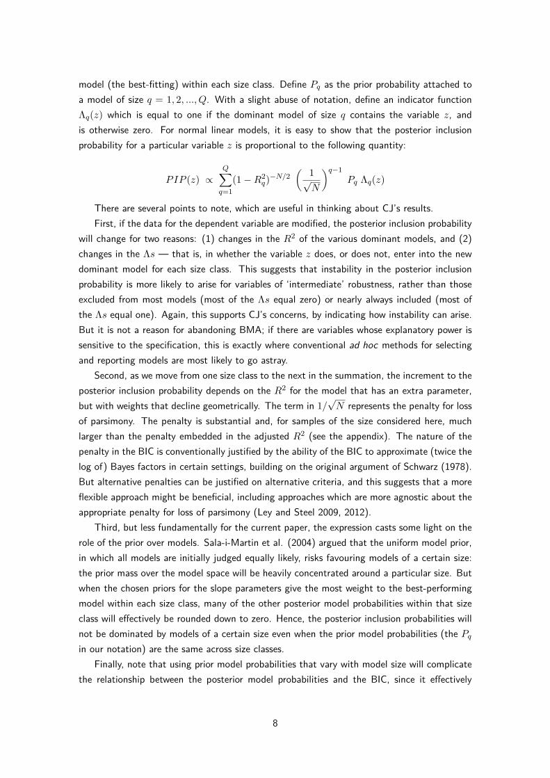
model (the best-fitting) within each size class. Define Pq as the prior probability attached toa model of size q = 1, 2, ..., Q. With a slight abuse of notation, define an indicator functionΛq(z) which is equal to one if the dominant model of size q contains the variable z, andis otherwise zero. For normal linear models, it is easy to show that the posterior inclusionprobability for a particular variable z is proportional to the following quantity:

PIP (z) ∝Q∑

q=1(1−R2

q)−N/2( 1√

N

)q−1Pq Λq(z)

There are several points to note, which are useful in thinking about CJ’s results.First, if the data for the dependent variable are modified, the posterior inclusion probability

will change for two reasons: (1) changes in the R2 of the various dominant models, and (2)changes in the Λs — that is, in whether the variable z does, or does not, enter into the newdominant model for each size class. This suggests that instability in the posterior inclusionprobability is more likely to arise for variables of ‘intermediate’ robustness, rather than thoseexcluded from most models (most of the Λs equal zero) or nearly always included (most ofthe Λs equal one). Again, this supports CJ’s concerns, by indicating how instability can arise.But it is not a reason for abandoning BMA; if there are variables whose explanatory power issensitive to the specification, this is exactly where conventional ad hoc methods for selectingand reporting models are most likely to go astray.

Second, as we move from one size class to the next in the summation, the increment to theposterior inclusion probability depends on the R2 for the model that has an extra parameter,but with weights that decline geometrically. The term in 1/

√N represents the penalty for loss

of parsimony. The penalty is substantial and, for samples of the size considered here, muchlarger than the penalty embedded in the adjusted R2 (see the appendix). The nature of thepenalty in the BIC is conventionally justified by the ability of the BIC to approximate (twice thelog of) Bayes factors in certain settings, building on the original argument of Schwarz (1978).But alternative penalties can be justified on alternative criteria, and this suggests that a moreflexible approach might be beneficial, including approaches which are more agnostic about theappropriate penalty for loss of parsimony (Ley and Steel 2009, 2012).

Third, but less fundamentally for the current paper, the expression casts some light on therole of the prior over models. Sala-i-Martin et al. (2004) argued that the uniform model prior,in which all models are initially judged equally likely, risks favouring models of a certain size:the prior mass over the model space will be heavily concentrated around a particular size. Butwhen the chosen priors for the slope parameters give the most weight to the best-performingmodel within each size class, many of the other posterior model probabilities within that sizeclass will effectively be rounded down to zero. Hence, the posterior inclusion probabilities willnot be dominated by models of a certain size even when the prior model probabilities (the Pq

in our notation) are the same across size classes.Finally, note that using prior model probabilities that vary with model size will complicate

the relationship between the posterior model probabilities and the BIC, since it effectively

8

alters the penalties for model complexity.5 When prior probabilities differ across models, thisimplies the Pq terms in the summation above will vary. This will make the posterior inclusionprobabilities more sensitive to the results of some model class sizes (those with high Pq) andless to others. It is possible that this could make the results more unstable, rather than less.Drawing on evidence from out-of-sample predictive performance and simulations, Eicher et al.(2010) argue that the uniform model prior works well. An alternative view, associated withFeldkircher and Zeugner (2009) and Ley and Steel (2009, 2012), is that it makes sense to usemore flexible priors in which the data are allowed to influence the penalty imposed on complexmodels, through the prior inclusion probabilities (Ley and Steel 2009) or the priors over slopecoefficients (Feldkircher and Zeugner 2009, Ley and Steel 2012). More flexible priors couldhelp to limit the instability identified by CJ, and we return to this issue later in the paper.

4 Results

Thus far, we have sketched some reasons why the theoretical arguments in Ciccone and Jaro-ciński (2010) are not conclusive, based on some additional considerations. But this raises anobvious question. If Bayesian Model Averaging is likely to be more robust than they suggest,how can we explain the results in their empirical application? Why do CJ find that growthregressions estimated using alternative vintages of the Penn World Table lead to very differentposterior inclusion probabilities?

Part of the explanation is that when CJ use different vintages, together with the largestpossible sample, the composition of the sample varies. This is examined by Feldkircher andZeugner (2012), who find that changes in the sample play an important role, not least becausethe countries which move in and out of the sample tend to be African ones that are especiallylikely to be outliers. Nevertheless, even after restricting attention to a fixed sample, someinstability remains. Feldkircher and Zeugner recommend the use of alternative priors, to limitthe importance of the supermodel effect. In particular, one aim of such priors, as in Ley andSteel (2009, 2012), is to increase robustness to prior assumptions, which in turn may limit theinstability that CJ identified.

The recent literature makes a strong case for using more sophisticated priors. Nevertheless,given that simpler priors continue to have some support (Eicher et al. 2010), and have beenwidely used in the empirical literature, it remains interesting to examine CJ’s results in moredetail. In the remainder of the paper we will argue that, even with inflexible priors, restrictingthe set of candidate models can greatly increase the stability of BMA results.

In particular, we think there is a strong case for requiring the candidate models to includeinitial GDP per capita and regional dummies. To see this, consider Table 2, which lists thefirst ten sets of posterior inclusion probabilities listed in Table 2 of CJ’s paper. An interestingfeature of this table is the posterior inclusion probability for the logarithm of initial (1960)

5See George and Foster (2000) for analysis of how the priors over models, and the priors over slope coeffi-cients, sometimes combine so that ranking by posterior model probabilities corresponds to ranking by variousformal model criteria.

9

Table 2: CJ posterior inclusion probabilitiesa

PWT 6.2 PWT 6.1 PWT 6.0

GDP per capita 1960 1.00 1.00 0.69Primary schooling 1960 1.00 0.99 0.79Fertility 1960s 0.91 0.12 0.03Africa dummy 0.86 0.18 0.15Fraction Confucius 0.83 0.12 0.20Fraction Muslim 0.40 0.19 0.11Latin American dummy 0.35 0.07 0.14East Asian dummy 0.33 0.78 0.83Fraction Buddhist 0.28 0.11 0.11Primary exports 1970 0.27 0.21 0.05a This table shows the first ten rows of PIPs from CJ (2010), theirTable 2.

GDP per capita. This has a posterior inclusion probability of 1.00 for PWT 6.1 and 6.2, butonly 0.69 in PWT 6.0. In other words, when a standard version of BMA is applied to the PWT6.0 data, more than 30% of the posterior mass is accounted for by models that exclude initialGDP per capita. Since initial GDP per capita is likely to be quite strongly correlated withsome of the candidate explanatory variables, this could be a source of instability in posteriorinclusion probabilities.

For a study of growth determinants, averaging across models which sometimes excludeinitial GDP per capita, and sometimes do not, is conceptually problematic. This is becausethe slope parameters have different economic interpretations, depending on whether or notinitial GDP per capita is included. Averaging the parameters becomes problematic, given thatthe economic interpretation of the parameters varies across models.6

To give a specific example, consider the empirical implications of the Solow model, asdeveloped in Mankiw et al. (1992). The model predicts that growth, measured over longtime periods, will be uncorrelated with investment rates: this is the famous result that thelong-run growth rate is independent of the investment rate. But when initial GDP per capita isincluded on the right-hand-side, the other right-hand-side variables do not have to be growthdeterminants: they can instead be variables which influence the height of the steady-stategrowth path. This set of variables could include, among others, the investment rate. A directconsequence is that, on standard theoretical grounds, the relevant set of predictors will dependon whether or not the regression controls for initial GDP per capita.

A more technical way to support this claim is to think about the underlying priors. Con-ceptually, the prior that a variable has a long-run growth effect is distinct from the prior thatit influences the height of the steady-state growth path. These differences in priors should

6In a related context, Hlouskova and Wagner (2013) have also noticed the importance of including initialGDP per capita in all models.

10

presumably be related to the strength of the researcher’s belief that endogenous growth mod-els (in which long-run growth effects are feasible) are likely to describe the data better thanneoclassical growth models in the traditions of Ramsey and Solow (in which long-run growtheffects are absent). If a model averaging exercise allows GDP per capita to move in and outof the candidate models, the two possibilities are conflated in ways that make the assumedpriors hard to justify.

A further issue is that a uniform model prior may be implausible in this context. That priorwill assign a prior probability of 0.5 to the inclusion of initial GDP per capita. In effect, endo-genous growth models with long-run growth effects, and neoclassical growth models withoutlong-run growth effects, are treated as equally likely before the data are analyzed. It is notclear that this prior reflects the current state of knowledge. Since the early work of Marris(1982), Kormendi and Meguire (1985), Baumol (1986), Barro (1991), Barro and Sala-i-Martin(1992) and Mankiw et al. (1992), empirical work on growth has routinely included a rolefor initial GDP per capita, and found it to be statistically significant. Under this approach,the explanatory variables are usually interpreted as giving rise to level effects — that is, theyinfluence the height of the steady-state growth path — rather than growth effects. Moreover,it is known that, in theoretical models, the existence of long-run growth effects typically relieson knife-edge parameter assumptions; hence, level effects seem more plausible than growtheffects.7 This paper proposes that, in order to ensure parameters can be given the sameeconomic interpretation across models, a model averaging exercise for growth should includeinitial GDP per capita in all the models considered. This can be justified partly on theoreticalgrounds, and partly by a large body of empirical work which finds initial GDP per capita toplay a role, at least once steady-state determinants are included.8

Further examination of Table 2 makes clear another reason for instability of the posteriorinclusion probabilities in CJ’s study. Many of the variables listed are dummies for regionsor dominant religion. There are several reasons why these variables could lead to instabilityin posterior inclusion probabilities. The most mechanical, although perhaps not the mostimportant, is that different combinations of region dummies can give rise to an artificial formof model uncertainty. First consider the extreme case where a set of R region fixed effectsis complete, in that each country is allocated to a region (as when zero/one region dummiessum to one for each country). Not all the region fixed effects can be included, given thepresence of an intercept. But there are several (in fact, R) statistically equivalent ways ofincluding R−1 region dummies, depending on which is the omitted region. Depending on thesoftware package, models that are statistically equivalent may be treated as different models.This will give rise to an artificial form of model instability; for example, the posterior inclusionprobabilities of the individual region dummies are likely to be unstable.9 A more general version

7These level effects may sometimes be large, and driven by the same mechanisms studied in endogenousgrowth models. Temple (2003) discusses these issues in more detail.

8This raises a deeper question: perhaps the parameters of interest in a model averaging exercise shouldbe the long-run effects, defined as the slope coefficients divided by the absolute size of the coefficient on thelogarithm of initial GDP per capita. Developing methods which define the priors over these long-run effectswould be an interesting area for further work.

9Software packages for BMA, including the original ‘bicreg’ software associated with Raftery et al. (1997)

11

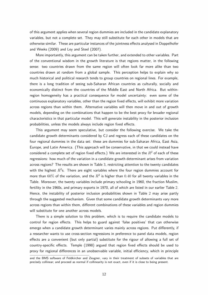
of this argument applies when several region dummies are included in the candidate explanatoryvariables, but not a complete set. They may still substitute for each other in models that areotherwise similar. These are particular instances of the jointness effects analysed in Doppelhoferand Weeks (2009) and Ley and Steel (2007).

More importantly, this argument can be taken further, and extended to other variables. Partof the conventional wisdom in the growth literature is that regions matter, in the followingsense: two countries drawn from the same region will often look far more alike than twocountries drawn at random from a global sample. This perception helps to explain why somuch historical and political research tends to group countries on regional lines. For example,there is a long tradition of seeing sub-Saharan African countries as culturally, socially andeconomically distinct from the countries of the Middle East and North Africa. But within-region homogeneity has a practical consequence for model uncertainty: even some of thecontinuous explanatory variables, other than the region fixed effects, will exhibit more variationacross regions than within them. Alternative variables will then move in and out of growthmodels, depending on the combinations that happen to be the best proxy for broader regionalcharacteristics in that particular model. This will generate instability in the posterior inclusionprobabilities, unless the models always include region fixed effects.

This argument may seem speculative, but consider the following exercise. We take thecandidate growth determinants considered by CJ and regress each of these candidates on thefour regional dummies in the data set: these are dummies for sub-Saharan Africa, East Asia,Europe, and Latin America. (This approach will be conservative, in that we could instead haveconsidered a complete set of region fixed effects.) We are interested in the R2 of each of theseregressions: how much of the variation in a candidate growth determinant arises from variationacross regions? The results are shown in Table 3, restricting attention to the twenty candidateswith the highest R2s. There are eight variables where the four region dummies account formore than 60% of the variation, and the R2 is higher than 0.40 for all twenty variables in theTable. Moreover, the twenty variables include primary schooling in 1960, the fraction Muslim,fertility in the 1960s, and primary exports in 1970, all of which are listed in our earlier Table 2.Hence, the instability of posterior inclusion probabilities shown in Table 2 may arise partlythrough the suggested mechanism. Given that some candidate growth determinants vary moreacross regions than within them, different combinations of these variables and region dummieswill substitute for one another across models.

There is a simple solution to this problem, which is to require the candidate models tocontrol for region effects. This helps to guard against ‘false positives’ that can otherwiseemerge when a candidate growth determinant varies mainly across regions. Put differently, ifa researcher wants to use cross-section regressions in preference to panel data models, regioneffects are a convenient (but only partial) substitute for the rigour of allowing a full set ofcountry-specific effects. Temple (1998) argued that region fixed effects should be used toproxy for regional differences in an unobservable variable, initial efficiency, which in principle

and the BMS software of Feldkircher and Zeugner, vary in their treatment of subsets of variables that areprecisely collinear; and proceed as normal if collinearity is not exact, even if it is close to being present.

12

Table 3: Proportion of variation in each variable explained by four region dummies.a

Variable R2

Fraction Population Over 65 .80Absolute Latitude .69Fraction Population Less than 15 .68Life Expectancy in 1960 .67Malaria Prevalence in 1960s .67Fertility in 1960s .62Political Rights .62Fraction of Tropical Area .62Fraction Population In Tropics .58Years Open 1950-94 .51Primary Schooling in 1960 .50Spanish Colony .49Fraction Muslim .48Higher Education 1960 .46Fraction Catholic .45Air Distance to Big Cities .44Civil Liberties .43Real Exchange Rate Distortions .43Ethnolinguistic Fractionalization .43Timing of Independence .42a This table reports the R2 of the regressionof each candidate variable on four regiondummies, for Sub-Saharan Africa, LatinAmerica, East Asia, and Europe.

should be included in conditional convergence regressions (see Mankiw et al. 1992 and Islam1995).

In a panel data setting, fixed effects are typically included because a researcher is concernedabout omitted variables, including omitted variables that may be difficult to measure or whoseimportance has not been appreciated by the researcher. Some of this logic can be extended to amodel averaging exercise. The set of candidate variables included in the analysis is likely to beincomplete. In the context of economic growth, a researcher can never rule out the possibilitythat a relevant variable has been omitted from the analysis. As Brock and Durlauf (2001)emphasize, growth theories are open-ended, in the sense that a role for one variable need notpreclude the existence of additional forces. If we take the view that at least some of theomitted variables are likely to vary substantially across regions, and less so within them, thenforcing the models to include region effects could help to address this point. We conjecturethat it will improve the performance of model averaging methods when the set of candidate

13

variables is incomplete.10

There are two main opposing arguments. First, when a researcher constructs regionalgroupings, this may draw on background knowledge of how different regions have grown,which could bias the results. From a statistical point of view, including a dummy based oncurrent membership of the OECD would be questionable, but defining regions on conventionalgeographic grounds is more defensible. Second, one might be concerned that including re-gion dummies means that the growth models speak to a different set of questions, and ruleout consideration of differences in outcomes across regions. Here, it is useful to distinguishbetween (1) what is identified, and (2) the sources of identifying variation. The inclusion ofregion-specific intercepts will often leave the economic interpretation of the slope parametersunchanged, but will use within-region variation to identify them.11 If a researcher remainsinterested in explaining differences in outcomes across regions, the slope parameters can becombined with the explanatory variables to shed light on this question. Easterly and Levine(1997, Tables VII.A and VII.B) is an example of this approach.

To examine the specific implications for CJ’s findings, we consider the following experiment.We investigate what CJ would have found, if they required every growth model to include initialGDP per capita and a small number of region fixed effects. We find that this would havereduced the number of growth determinants found to be robust, and would have drasticallyreduced the instability of posterior inclusion probabilities across different vintages of the PWT.Moreover, these results continue to apply when we go further than CJ, and consider vintagesof the PWT that were not available to them at the time of their study. Hence, we show thatmodifying the set of candidate models — in particular, reducing the degree of agnosticism, byrequiring some variables to appear in each model — should help to limit the number of falsepositives that might otherwise emerge.

We will present this result in several different ways. As in CJ, our focus is not on theinterpretation of the posterior inclusion probabilities of specific regressors, and we are nottrying to derive new findings on the determinants of growth. Rather, we examine whetherconditioning on initial GDP per capita and regional fixed effects helps to limit instability in theposterior inclusion probabilities. Our first yardstick will be the number of variables which are‘robust’, those where the posterior inclusion probability exceeds the prior inclusion probability;this criterion is used in Sala-i-Martin et al. (2004). How does the set of robust variableschange across PWT vintages? More precisely, how many variables are robust for at least onePWT vintage, but not all?

These numbers are reported in Table 4.12 We report two sets of results, one based on the10This perspective acknowledges that, in the growth setting, the true data generating process is unlikely to

be among the models considered, even when the number of candidate models is very large. This raises thequestion of whether AIC-based methods for model averaging are worth exploring; see Burnham and Anderson(2002, 2004) and Claeskens and Hjort (2008).

11In much the same way, panel data estimation of the Solow model with country fixed effects (for example,Islam 1995) uses within-country variation to identify the same structural parameters as the cross-section studyof Mankiw et al. (1992).

12These and the other BMA results in the paper were obtained using the BMS software due to Feldkircherand Zeugner.

14

same three vintages used in CJ, and the other augmenting their dataset with the later PWTversions 6.3, 7.0, 7.1, and 8.0. We use the BRIC prior of Fernández et al. (2001b) for thecoefficients within each model, and a Bernoulli prior over models where the expected modelsize is seven variables, as in Sala-i-Martin et al. (2004). The ‘CJ’ column shows the largenumber of variables that emerge as robust in one PWT vintage but not in another; this is onereflection of the instability that concerns CJ. The next column restricts attention to conditionalconvergence regressions (those conditioning on initial GDP per capita, Y0). This reduces theinstability, but less than might have been expected.

Next, we add a small set of region fixed effects: to maintain comparability with previouswork, we use the regional dummies that were included in the Sala-i-Martin et al. (2004)analysis. These are dummies for sub-Saharan Africa, East Asia, Europe, and Latin America.The results are stark: the number of variables which are robust at least once, but not always,is reduced by nearly 80 percent. Allowing for the identity of colonial powers (the final column)results in little further improvement, and for vintages 6.0-8.0, actually increases instability.

Table 4: Model Stability Comparisonsa

CJ Y0 Y0 & Continents Y0 & Continents & Colonial Powers

PWT 6.0-6.2 19 15 4 3

PWT 6.0-8.0 24 22 6 7a This table reports the number of variables that are ‘robust’ (see text) for at least one vintageof the PWT but not all. Column CJ refers to the approach of Ciccone and Jarociński (2010).The next columns require all models to include initial GDP per capita, Y0; initial GDP percapita and four region dummies; initial GDP per capita, four region dummies, and dummiesfor colonial powers. The first row uses the three vintages of the PWT considered by CJ; thesecond adds four subsequent vintages, up to the PWT 8.0 release.

Taken together, these results point clearly in one direction. Growth studies are more likelyto deliver reliable findings if the candidate models are required to include GDP per capita andregion fixed effects. We now provide an alternative summary of the results, which gives moreinsight into the extent and nature of the improvements in stability. By studying the distributionof the changes in posterior inclusion probabilities, we find evidence that the inclusion of initialGDP capita matters more than Table 4 implies. But the most important finding is that,by including region fixed effects, stability across vintages is greatly improved, because fewergrowth determinants are ever assigned a high posterior inclusion probability.

One reason that a more detailed presentation is useful is that posterior inclusion probabilitiescould display relatively small changes across vintages, and thereby give rise to the apparent lackof robustness highlighted in Table 4. CJ are careful to address this, and show that their resultsare not simply driven by modest changes either side of thresholds. In our investigation, we nowconsider a summary measure MAXDIFF (z). This is defined, for each candidate explanatoryvariable z, as the difference between the maximum and minimum posterior inclusion probability

15

across vintages of the PWT:

MAXDIFF (z) ≡Maxi

PIPi(z)−Minj

PIPj(z)

where i and j index vintages of the PWT. By construction, MAXDIFF (z) is boundedbetween zero and one. A high value for a given variable suggests that the posterior inclusionprobability of that variable is especially sensitive to the data employed; a value close to zerosuggests the posterior inclusion probabilities are relatively stable. Hence, a distribution ofMAXDIFF (z) that has more mass close to zero indicates a relatively stable set of findings.

Figure 1: Maximum Difference in Posterior Inclusion Probabilities across PWT 6.0 — 6.2

●

●

●●

●●

●

●

●●

●

●

●

●

●

●●

●

●

●

●

●

●

●

●

●

●

●

●●

●

●

●

●

●

●0.25

0.50

0.75

1.00

0.00 0.25 0.50 0.75 1.00Maxdiff

P(x

<X

)

CJ's Results (their Table 2)

●

●

●

●

●

●

●

●

●

●

●

●

●

●

●

●

●

●

●

●

●

●

●

●

●

●

●

●●

●

●

●

●

●

●

●

●

●●

●

●●

●

●

●●

●

●●

●

●

●

●

●

●●●

●

●●

●

●

●

●

●

●

●0.00

0.25

0.50

0.75

1.00

0.00 0.25 0.50 0.75 1.00Maxdiff

P(x

<X

)

y0 Only

●

●

●●

●

●

●

●

●●

●

●

●

●

●

●

●

●

●

●

●●

●

●

●

●

●

●

●

●

●

●

●

●

●

●

●

●

●

●●

●

●

●●

●

●

●

●

●

●

●●

●

●●

●●

●

●●●

●

0.25

0.50

0.75

1.00

0.00 0.25 0.50 0.75 1.00Maxdiff

P(x

<X

)

y0 and Continent Dummies

●

●

●

●

●

●

●

●

●

●

●

●

●

●

●

●

●

●

●

●

●

●

●●

●

●

●

●

●

●●

●

●

●

●

●

●●

●

●

●●

●●

●

●

●

●

●

●

●

●

●

●

●

●

●

●

●

●0.25

0.50

0.75

1.00

0.00 0.25 0.50 0.75 1.00Maxdiff

P(x

<X

)

y0 and Continent and Colony Dummies

Figures report the empirical CDF of the maximum difference in PIPs across PWT vintages.

The top-left panel of Figure 1 plots the empirical cumulative distribution function (CDF)of MAXDIFF (z) for the results reported by CJ in their Table 2. The largest observed valuesof MAXDIFF (z) are surprisingly close to one, which might be explained by collinearitybetween, for example, different measures of population density or dummy variables. It is notclear how general this explanation can be, however. The 75th percentile of MAXDIFF (z)is close to 0.25, and so a major change in posterior inclusion probabilities across vintages —a change larger than 0.25 — is observed for more than a quarter of the candidate growthdeterminants.

The top-right panel repeats this analysis, but this time requiring initial GDP per capita Y0

to be included in all the models. Now the maximum of MAXDIFF (z) is below 0.75 and,more importantly, the 75th percentile is only 0.09: so for three-quarters of the variables, the

16

change in the posterior inclusion probability across vintages is now less than 0.10. The lowerpanels add region fixed effects (bottom-left) and also dummies for the former colonial power(bottom-right). These panels show a pronounced reduction in the number of large changes,with the CDF moving much closer towards the y-axis.

Given that later vintages of the PWT have been released since CJ wrote their paper, we askwhether extending their analysis to these additional vintages gives similar results. The top-leftpanel of Figure 2 displays the empirical CDFs of MAXDIFF (z) based on differences acrossfour newer vintages of the PWT, 6.3, 7.0, 7.1 and 8.0. These results are quite close to thosein the top-left panel of Figure 1. But again, the instability is reduced by the inclusion of initialGDP per capita and region fixed effects in all models. The main departure from the previousresults is that including dummies for the former colonial power (the bottom-right panel) is amore noticeable improvement.

Figure 3 considers the same four cases as Figure 2, but now MAXDIFF (z) is calculatedacross seven vintages of the PWT. By construction, considering a larger number of vintagescannot reduce MAXDIFF (z). Put differently, on this metric, the instability that CJ identifycan only get worse as the PWT data are repeatedly updated and revised, unless a researchercan confidently identify some vintages as more reliable than others. But Figure 3 shows thesame overall pattern: instability is sharply reduced by forcing the inclusion of initial GDPcapita, region fixed effects, and dummy variables for former colonial powers.

We now briefly investigate a related issue: as Feldkircher and Zeugner (2012) emphasize,the posterior inclusion probabilities are unstable across vintages in CJ partly because the setof countries varies. The countries which move in and out of the sample are disproportionatelypoor and/or in sub-Saharan Africa. With this in mind, we repeat our experiment using a fixedsubsample of 75 countries, initially studying vintages 6.0, 6.1, and 6.2. We use a new styleof figure, which also plots the minimum and maximum posterior inclusion probability for eachvariable, linking the extremes with a horizontal bar for ease of interpretation. This is shownin Figure 4, with a vertical line at a posterior inclusion probability of x = 7/67, representingthe Sala-i-Martin et al. (2004) criterion for deeming a result to be of interest. The longhorizontal bars in the top-left panel show the considerable instability in the posterior inclusionprobabilities highlighted by CJ. The seven variables identified as robust by CJ are those forwhich both the maximum and minimum are to the right of the vertical line.

The other panels show the difference made by a fixed sample (top-right), the inclusion ofinitial GDP per capita (bottom-left) and the inclusion of initial GDP per capita and regionfixed effects (bottom-right). In the latter case, there is an especially clear partition of thevariables into those which potentially matter, and those which appear in relatively few well-performing models: most of the horizontal bars are much shorter than before. This suggeststhat, as anticipated, the inclusion of region fixed effects helps to guard against potential falsepositives.

A remaining question is whether any variables emerge as consistently important. Table 5shows the minimum, median and maximum posterior inclusion probability for the four variableswhose posterior inclusion probability exceeds the 7/67 threshold across three vintages of the

17

Figure 2: Maximum Difference in Posterior Inclusion Probabilities across PWT 6.3—8.0

●

●

●

●

●

●

●

●

●

●

●

●

●

●

●

●

●

●

●

●

●

●

●

●

●

●

●

●

●

●

●

●

●

●

●

●

●

●

●

●●

●

●

●

●

●

●

●

●

●

●

●

●

●

●

●

●

●●

●

●

●

●

●

●

●

●

0.00

0.25

0.50

0.75

1.00

0.00 0.25 0.50 0.75 1.00Maxdiff

P(x

<X

)Specification as in CJ

●

●

●

●

●

●●

●

●

●

●●

●

●

●

●

●

●

●

●

●

●

●

●

●●

●

●

●

●

●

●

●

●

●

●

●

●

●

●●

●

●

●

●

●

●

●

●●

●

●

●

●

●

●

●

●●

●

●

●

●

●

●

●

●0.00

0.25

0.50

0.75

1.00

0.00 0.25 0.50 0.75 1.00Maxdiff

P(x

<X

)

y0 Only

●

●

●

●

●

●

●

●

●

●

●

●

●●

●

●

●

●

●

●

●

●

●

●

●

●

●

●●

●

●

●

●●

●

●

●

●

●

●

●

●

●

●

●

●

●

●

●

●

●

●

●

●●

●

●

●

●

●●

●●

0.25

0.50

0.75

1.00

0.00 0.25 0.50 0.75 1.00Maxdiff

P(x

<X

)

y0 and Continent Dummies

●

●

●

●

●

●

●

●

●

●

●

●

●

●

●

●

●●

●

●

●

●

●

●

●

●

●

●

●

●

●

●

●

●

●●

●

●

●

●

●

●

●

●

●

●

●

●

●

●

●

●

●

●

●

●

●

●

●

●

0.25

0.50

0.75

1.00

0.00 0.25 0.50 0.75 1.00Maxdiff

P(x

<X

)y0 and Continent and Colony Dummies

PWT, when initial GDP and four region fixed effects are included. In several cases, the variationemphasized by CJ remains visible. But the evidence that primary schooling in 1960 matters isstrong: its posterior inclusion probability is close to unity across three vintages of the PWT.Put differently, those models which exclude initial primary schooling are all assigned very lowposterior model probabilities. Given that the benefits of education for growth have often beencontested, this is a striking result.

Table 5: PIPs for robust variables based on fixed sample PWT 6.0—6.2 a

Minimum PIP Median PIP Maximum PIP

Primary Schooling in 1960 0.99 1.00 1.00Fertility 1960s 0.13 0.61 0.74Primary Exports 1970 0.15 0.43 0.59Fraction Confucius 0.18 0.27 0.39

The remaining problem is that these findings do not extend to more recent vintages of thePWT. We repeat the above analysis for the four subsequent vintages of the PWT available

18

Figure 3: Maximum Difference in Posterior Inclusion Probabilities across PWT 6.0—8.0

●

●

●

●

●

●

●

●

●

●

●

●

●

●

●

●

●

●

●

●

●

●

●

●●

●

●

●

●

●

●

●

●

●

●

●●

●●

●

●●

●

●

●

●

●

●

●

●

●

●

●

●

●

●

●●

●●

●

●

●

●

●

●

●0.00

0.25

0.50

0.75

1.00

0.00 0.25 0.50 0.75 1.00Maxdiff

P(x

<X

)Specification as in CJ

●

●

●

●

●

●

●

●

●

●

●●

●

●

●

●

●

●

●

●

●

●

●

●

●●

●

●

●

●

●

●

●

●

●

●●

●

●

●

●●

●

●

●

●

●

●●

●

●

●

●

●

●

●

●●

●●

●

●

●

●

●

●

●0.00

0.25

0.50

0.75

1.00

0.00 0.25 0.50 0.75 1.00Maxdiff

P(x

<X

)

y0 Only

●

●

●

●

●

●

●

●

●

●

●

●

●●

●

●

●

●

●

●●

●

●

●

●

●●

●

●

●

●

●

●

●

●●

●

●

●

●

●

●

●

●

●

●

●

●

●

●

●

●

●

●

●●

●

●

●

●●

●

●

0.25

0.50

0.75

1.00

0.00 0.25 0.50 0.75 1.00Maxdiff

P(x

<X

)

y0 and Continent Dummies

●

●

●

●

●

●

●

●

●

●

●

●

●

●

●

●

●●

●

●

●

●

●●

●

●

●

●

●

●●●

●

●

●

●

●

●

●

●

●

●

●

●

●

●

●

●

●

●

●

●

●●

●

●

●●

●

●

0.25

0.50

0.75

1.00

0.00 0.25 0.50 0.75 1.00Maxdiff

P(x

<X

)y0 and Continent and Colony Dummies

to us, with results reported in Table 6. The fixed sample of countries differs, but otherwise,only the vintages of the PWT vary between the two Tables. The variables which emerge asconsistently ‘robust’ are now somewhat different, and the variables previously identified asrobust (shown in the last four rows) now have rather variable inclusion probabilities. In termsof substantive conclusions about growth, the alternative sets of variables listed in Tables 5 and6 point to factors that are widely associated with East Asia’s rapid growth — even thoughwe are controlling for an East Asian dummy in these models. Put differently, past emphasison growth-promoting aspects of East Asia’s initial conditions and subsequent policies, such ashigh primary schooling, low specialization in primary exports/mining, and relatively open tradepolicies, may have been on the right track. But as Table 6 indicates, it is difficult to inferwhich of these forces matter most, as CJ would have anticipated.

It is clear that when initial GDP per capita and region fixed effects are always includedin the models, the list of other growth determinants consistently identified by BMA is short,especially compared to the many candidates that have been considered. Our findings in thisregard are consistent with CJ’s overall conclusion, quoted earlier in this paper, that the datauncertainties may be too great to identify more than a small number of growth determinants.

19

Figure 4: Posterior Inclusion Probabilities across PWT Vintages 6.0 — 6.2

●●●●●

●●

●

●●●

●●

●

●●

●

●

●●●

●

●

●

●

●

●

●

●

●●●●

●

●

●●

●●●●

●

●

●

●

●

●

●

●

●

●●●

●

●

●●

●

●

●

●

●●

●

●●

●

0.25

0.50

0.75

1.00

0.00 0.25 0.50 0.75 1.00Maximum PiP

P(x

<X

)

Specification as in CJ

●

●

●

●

●

●

●

●

●

●

●

●

●

●

●

●

●

●●

●

●

●

●

●●

●

●

●●●

●

●

●

●

●

●

●

●

●

●●

●

●

●

●

●

●

●

●

●

●

●●

●

●

●

●

●

●

●

●●

●

●

●

●

●

0.00

0.25

0.50

0.75

1.00

0.00 0.25 0.50 0.75 1.00Maximum PiP

P(x

<X

)

Fixed Sample

●

●

●

●

●

●

●

●

●

●

●

●

●

●

●

●

●

●

●

●

●

●

●

●●

●

●

●

●●

●

●

●

●

●

●

●

●

●

●

●

●

●

●

●

●

●

●

●

●

●●●

●

●

●

●●

●

●

●●

●

●

●

●

●

0.00

0.25

0.50

0.75

1.00

0.00 0.25 0.50 0.75 1.00Maximum PiP

P(x

<X

)

y0 Only

●

●

●

●●●

●

●

●

●

●

●●

●

●

●

●●

●

●

●

●

●●

●

●

●

●

●●

●●

●●

●●●

●

●

●

●

●

●

●●

●

●

●

●

●

●

●

●

●●

●

●●

●

●

●●

●

●

●

●

●

0.00

0.25

0.50

0.75

1.00

0.00 0.25 0.50 0.75 1.00Maximum PiP

P(x

<X

)

y0 and Continent Dummies

The figures show the empirical CDF of the maximum PIP across PWT vintages. In addition, horizontal barsextend between the minimum and maximum PIP for each variable. The vertical line, x = 7/67, is the Sala-i-Martin et al. (2004) threshold for a variable to be considered robust.

Researchers who begin as agnostics may be destined to remain as agnostics.In their own extension of the CJ results, Feldkircher and Zeugner (2012) similarly conclude

in favour of ‘robust ambiguity’. They find that, when using a hierarchical prior which allowsmore flexibility in the extent of shrinkage, the posterior mass is distributed more evenly acrosscandidate models. This reduces the variation of posterior inclusion probabilities across vintagesof the PWT data, but also reduces the variation across variables for a given vintage. Thatfinding raises the following question: if we combine their priors with the ideas of this paper,and restrict the model space, can we start to discriminate more readily between variables?

To investigate this, we follow them in using a uniform model prior, but a flexible ‘hyper-g’prior for the coefficients in each model. This allows the extent of shrinkage to be influencedby the data, and should make the analysis less dependent on prior assumptions, which areinevitably arbitrary to some degree. Hierarchical priors of this general form are among thoseconsidered by Feldkircher and Zeugner (2009), Ley and Steel (2012), and Liang et al. (2008).Ley and Steel (2012) provide further references, and note that the effect is to extend theconventional g-prior to be a mixture of normals, with more flexible tails than a normal distri-bution. For comparability with Feldkircher and Zeugner (2012), we set the expected extentof shrinkage (the mean of the prior over the ‘g’ parameter) equal to the (fixed) extent ofshrinkage found in the benchmark BRIC prior of Fernández et al. (2001b).

20

Table 6: PIPs for robust variables based on fixed sample PWT 6.3—8.0 a

Minimum PIP Median PIP Maximum PIP

Life Expectancy in 1960s 0.34 0.63 0.78Mining as a Percentage of GDP 0.17 0.94 0.99Openness 1965-1974 0.17 0.31 0.43

Primary Schooling in 1960 0.08 0.37 0.56Fertility 1960s 0.07 0.14 0.24Primary Exports 1970 0.07 0.17 0.21Fraction Confucius 0.03 0.19 0.25

The results for version 8.0 of the PWT are shown in Table 7. Here, we are less interestedin variability across vintages of the data. Instead, we want to know how the posterior inclusionprobabilities vary, under flexible priors, or flexible priors with some variables always included.With this in mind, the table reports some of the percentiles of the PIP distribution, and theinterquartile range (IQR). The table shows that forcing the models to include initial GDP percapita slightly raises the interquartile range; then, additionally forcing the models to includeregion fixed effects lowers the interquartile range substantially. But the latter effect arisesbecause many of the posterior inclusion probabilities are moved closer to zero. The numberof candidate variables with an inclusion probability greater than 7/67 (see the final row of thetable) is now rather small. Similar results apply for earlier vintages of the PWT data (resultsnot reported). These results show that our main points — the need to include initial GDPper capita, and region dummies — have implications for the results even when a hyperprior isused; and that the method does isolate a limited number of variables as more important thanothers. The results also continue to suggest, in line with CJ, that most of the variables do nothave much support from the data.

Table 7: Percentiles for PIP distribution — PWT 8.0a

Percentile Hyper-g Hyper-g & Y0 Hyper-g & Y0 & Continents

0.25 0.06 0.05 0.020.50 0.08 0.06 0.030.75 0.15 0.14 0.050.90 0.26 0.24 0.15

IQR 0.085 0.090 0.032No.PIP ≥ 7/67 20 18 7a This table shows the percentiles of the PIP distribution for PWT 8.0, when a hyper-gprior is used, and then when initial GDP per capita is always included, and then wheninitial GDP per capita and region dummies are always included. In each case, the PIPdistribution is for a fixed set of variables, excluding GDP per capita and the regiondummies.

21

This does not mean that nothing matters, however. Interestingly, in these results basedon a hyper-g prior, the one variable which repeatedly emerges with a high posterior inclusionprobability is the primary school enrollment rate in 1960. In one sense, this is not a new result; itis one of the variables emphasized most by Sala-i-Martin et al. (2004), given its high posteriorinclusion probability in their study. Before them, Levine and Renelt (1992) had identifiedan alternative measure of mass education — the secondary school enrollment rate — as anunusually robust determinant of growth. Now, with additional vintages of data, and improvedmethods for addressing model uncertainty, it seems clear that both sets of authors were rightto draw attention to schooling. It is especially important given the long-standing debate overwhether donors and developing-country governments should prioritize growth or meeting basicneeds; broad-based schooling can address both.13 That seems well worth knowing, and initself, worth the energy that has been expended upon these methods.

5 Discussion

We now discuss some broader issues. For its detractors, the empirical growth literature isoften said to ask questions of the data that the data are ill-equipped to answer. The criticshave found support, at least indirectly, in the work of Jerven (2013). He points to the manyproblems with national accounts statistics in sub-Saharan Africa, raising doubts about what canbe learnt from the data. It is interesting to ask whether the issues identified by CJ are primarilythe weaknesses of (one version of) BMA, or weaknesses that arise from mismeasurement.

Perhaps inevitably given the complexity of the exercise, at least some versions of the PWThave contained errors. Jerven (2013, pp. 70-71) discusses a major problem with the PWT 6.1data on GDP for Tanzania, while Dowrick (2005) uncovered errors in PWT 6.1 data on labourforce participation rates for around 15 countries in sub-Saharan Africa. More fundamentally,the compilers of the PWT have had to face difficult choices about how to use the price datafrom multiple benchmark years, and how to construct PPP estimates for countries where ICPbenchmark data are not available. In practice, this means that the data revisions across PWTvintages can be significant, as Johnson et al. (2013) analyze in detail. But they also findthat the conclusions of some prominent studies are quite robust, especially when studies arebased on growth rates calculated over long spans of time, rather than making intensive use ofthe high-frequency variation. They conclude ‘whatever else is right or wrong with the growthliterature, the bulk of it is not afflicted by the problem of sensitivity to changes in PWT GDPdata’ (Johnson et al. 2013, p. 266).

Their findings suggest that the instability of BMA cannot be attributed solely to weaknessesin the data. It remains possible that BMA, in the forms implemented here, is too sensitiveto small changes in the sample, perhaps because of the effects of outliers. In the case of aBIC-based approach, this would not be a surprise: in the normal linear model, the BIC can

13It could be objected that this is only a statistical association, not a causal effect, and that Bils and Klenow(2000) provide an alternative explanation for the association. But views will differ on its plausibility, and itseems hard to argue that someone new to this literature should not update their priors.

22

be written as a function of the R2, and the R2 is a highly non-robust statistic. More generally,most Bayesian approaches to model averaging rely on the sum of squared errors as the measureof fit, and this is similarly non-robust. The simulations in Machado (1993) indicated that fat-tailed error distributions induce a tendency for the BIC to select models which are too small.Machado introduced an approach for making the BIC outlier-robust; see also Claeskens andHjort (2008, pp. 81-82). In principle, the weights used in model averaging could be basedon statistics that are more robust than the BIC, and this idea seems worth pursuing infuture work. So does the simpler approach of drawing conclusions based on repeatedly takingsubsamples from the data. This method is adopted in Ley and Steel (2009, 2012) and shouldarguably become standard in future studies that use model averaging.

It is worth noting that outlier-robustness is a consideration even with a fixed sample,because the influence exerted by outliers will change with each model considered. If we thinkof outliers as observations that are generated from a distinct data-generating process, perhapsone of secondary interest, the extent to which these observations are well approximated willvary across models. This raises the possibility that certain models have high posterior modelprobabilities mainly because a particular combination of variables captures data variation that,in a more robust analysis, would have been identified as atypical. Ideally, variable selectionor model averaging require the simultaneous consideration of outliers, especially in samples ofthe size considered here; see Temple (2000) for further discussion and references.

This can be extended to a broader criticism of model averaging as usually implemented byeconomists. Statisticians have often made the point that model criticism or model checkingis a fundamental component of empirical research. In contrast, most of the applications ofBMA by economists are a little mechanical in this regard, with limited use of plots of thedata, or careful study of the properties of individual models. Our aim has been to study thesensitivity of BMA rather than derive a set of substantive conclusions about growth; a carefulinvestigation of the latter would need to take a more flexible, iterative approach to aspects ofthe data and the specification.14

This relates to another broad point, namely the underlying aims of using BMA. One reasonfor using Bayesian approaches is that conventional significance tests are rarely a sound basis onwhich to form policy or take decisions, as Brock and Durlauf (2001) and Brock et al. (2003)emphasized.15 In this paper, we have followed much of the growth literature in emphasizingposterior inclusion probabilities. One justification is that a theorist might be interested inknowing which variables appear to influence growth, while taking a conservative approachthat is wary of ‘false positives’. For policy-makers, however, the posterior distributions of theparameters are especially relevant, arguably more so than the posterior inclusion probabilities.It would be possible for a posterior distribution to have substantial mass at zero, but also to

14On Bayesian methods for model checking and sensitivity analysis, see chapters 6 and 7 of Gelman et al.(2014). Gelman and Shalizi (2013) discuss the place of these methods within a wider philosophy of statistics.

15A principal theme of McGrayne (2011) is that Bayesian principles have often been successful in practicalapplications for which classical methods are either ill-equipped or actively misleading. For accounts of decisiontheory linked to Bayesian principles, see chapter 9 of Gelman et al. (2014), or Leonard and Hsu (1999). Kass(2011) gives an account of the pragmatism of modern statistical practice.

23

assign sufficient mass to large negative or positive effects (or both) that the variable becomeshighly relevant to a policy decision.

This suggests that an especially interesting sequel to Ciccone and Jarociński would be toreframe the problem in terms of a policy decision, and examine its sensitivity to the use ofalternative vintages of data. We leave this as an idea for further work, but note that oncepolicy decisions become the central focus, it is less clear that region fixed effects should beincluded in every model considered, and one might also want to assign at least a little priorprobability to the existence of long-run growth effects.

6 Conclusions

At least in economics, it seems likely that many published findings are based at least partly ondata mining and ‘directed’ model searches. Even those researchers who adopt a more agnostic,open-minded approach rarely take model selection into account when carrying out inference.These problems suggest that model selection, estimation, and inference should be consideredjointly. Over the last twenty years, Bayesian Model Averaging has emerged as an attractiveapproach, and one which is increasingly easy to implement. In this paper, we have examinedone of the most important critiques of BMA, that advanced by Ciccone and Jarociński (2010).

We revisit their theoretical arguments, and note some additional considerations that qualifythe arguments a little. We also reconsider their empirical analysis. In particular, we showthat instability in posterior inclusion probabilities is sharply reduced by restricting the set ofcandidate models, so that initial GDP per capita and a small set of region fixed effects areincluded in each model. There are theoretical arguments for requiring these particular variablesto be included. Moreover, we find that their inclusion enhances robustness even when weextend the analysis to more recent vintages of the Penn World Table, not studied by CJ. Formany variables, the posterior inclusion probabilities do not vary widely across vintages of thePWT, calling into question the generality of some of the points made by CJ. But in closeragreement with CJ, we also find that few variables are consistently identified as importantgrowth determinants. Our restriction of the model space works mainly because high posteriorinclusion probabilities become less common.

As this suggests, many of the points made by CJ have some force. Even using the approachwe have recommended in this paper, there remains some instability across data vintages,suggesting that they were correct to raise concerns. It is likely that future research will drawon newer methods, especially more flexible priors, such as those advocated by Feldkircher andZeugner (2009) and Ley and Steel (2012). In the meantime, attention to the set of candidatemodels is likely to bring significant benefits; one can have too much agnosticism. Our resultssuggest that cross-section growth regressions should routinely include initial GDP per capitaand region fixed effects, whether or not model averaging is used.

24

7 Appendix

We briefly discuss the penalty for loss of parsimony embedded in the BIC approach. Using thedefinition of the adjusted R2 as:

R2q ≡ 1−

(N − 1

N − q − 1

)(1−R2

q)

we can rewrite the posterior inclusion probability (for the normal linear model, with one modelper size class) in terms of each dominant model’s adjusted R2:

PIP (z) ∝Q∑

q=1(1−R

2q)−N/2 ωq Pq Λq(z)

where the weights ωq are

ωq ≡(

1− 1 + q

N

)−N/2 (1− 2

N

)N/2N−(q−1)/2

For N = 88, the sample size in Sala-i-Martin et al. (2004), the weights decline rapidly,in the ratio of approximately 5 : 1. In other words, in computing the posterior inclusionprobability, the BIC approach will not give much weight to larger models unless they increasethe adjusted R2 substantially. This reflects a well-known property of the BIC penalty for modelsize: it is much stricter than the penalty embedded in the adjusted R2. Kuha (2004, p. 216)gives an especially clear account of the reasons for favouring parsimony.

References

[1] Amini, S. and Parmeter, C. F. (2012). Comparison of model averaging techniques: as-sessing growth determinants. Journal of Applied Econometrics, 27, 870-876.

[2] Banerjee, A. V. (2009). Big answers for big questions: the presumption of growth policy.In J. Cohen and W. Easterly (eds.) (2009). What works in development? Thinking bigand thinking small. Brookings Institution Press, Washington DC.

[3] Barro, R. J. (1991). Economic Growth in a Cross Section of Countries. Quarterly Journalof Economics, 106(2), 407-43.

[4] Barro, R. J. and Sala-i-Martin, X. (1992). Convergence. Journal of Political Economy,100(2), 223-51.

[5] Bartelsman, E. J. and Wolf, Z. (2014). Forecasting aggregate productivity using inform-ation from firm-level data. Review of Economics and Statistics, 96, 745-755.

[6] Baumol, W. J. (1986). Productivity Growth, Convergence, and Welfare: What the Long-run Data Show. American Economic Review, 76(5), 1072-1085.

25

[7] Begun, J. and Eicher, T. (2008). In Search of a Sulphur Dioxide Environmental KuznetsCurve: A Bayesian Model Averaging Approach. Environment and Development Econom-ics, 13(6), 1-28.

[8] Bils, M. and Klenow, P. J. (2000). Does schooling cause growth? American EconomicReview, 90(5), 1160-1183.

[9] Breiman, L. (1992). The little bootstrap and other methods for dimensionality selectionin regression: X-fixed prediction error. Journal of the American Statistical Association,87, 419, 738-754.

[10] Brock, W. A. and Durlauf, S. N. (2001). Growth Empirics and Reality. World BankEconomic Review, 15(2), 229-272.

[11] Brock, W. A., Durlauf, S. N., and West, K. D. (2003). Policy Evaluation in UncertainEconomic Environments. Brookings Papers on Economic Activity, 34(1), 235-322.

[12] Brodeur, A., Lé, M., Sangnier, M. and Zylberberg, Y. (2013). Star Wars: the empiricsstrike back. Manuscript, Paris School of Economics, March.

[13] Burnham, K. P. and Anderson, D. R. (2002). Model Selection and Multimodel Inference(second edition). Springer.

[14] Burnham, K. P. and Anderson, D. R. (2004). Multimodel inference: understanding AICand BIC in model selection. Sociological Methods & Research, 33, 261-304.

[15] Ciccone, A. and Jarociński, M. (2010). Determinants of economic growth: will data tell?American Economic Journal: Macroeconomics, 2(4), 222-246.

[16] Claeskens, G. and Hjort, N. L. (2008). Model Selection and Model Averaging. CambridgeUniversity Press, Cambridge.

[17] Cohen-Cole, E. B., Durlauf, S. N. and Rondina, G. (2012). Nonlinearities in growth: fromevidence to policy. Journal of Macroeconomics, 34, 42-58.

[18] Crainiceanu, C. M., Dominici, F. and Parmigiani, G. (2008). Adjustment uncertainty ineffect estimation. Biometrika, 95(3), 635-651.

[19] Crespo Cuaresma, J., Doppelhofer, G. and Feldkircher, M. (2014). The determinants ofeconomic growth in European regions. Regional Studies, 48, 44-67.

[20] Danquah, M., Moral-Benito, E., and Ouattara, B. (2014). TFP growth and its determin-ants: a model averaging approach. Empirical Economics, 47, 227-251.

[21] Davidson, R. and MacKinnon, J. G. (1993). Estimation and inference in econometrics.Oxford University Press, Oxford.

26

[22] Deckers, T. and Hanck, C. (2014). Variable Selection in Cross-Section Regressions: Com-parisons and Extensions. Oxford Bulletin of Economics and Statistics, 76, 841-873.

[23] Doppelhofer, G. and Weeks, M. (2009). Jointness of growth determinants. Journal ofApplied Econometrics, 24(2), 209-244.

[24] Doppelhofer, G. and Weeks, M. (2011). Robust Growth Determinants. CESifo WorkingPaper Series No. 3354.

[25] Dowrick, S. (2005). Errors in the Penn World Table demographic data. Economics Letters,87, 243-248.

[26] Durlauf, S. N., Fu, C. and Navarro, S. (2012). Assumptions matter: model uncertaintyand the deterrent effect of capital punishment. American Economic Review, Papers andProceedings, 102(3), 487-492.

[27] Easterly, W. (2009). Comment on Banerjee. In J. Cohen and W. Easterly (eds.) (2009).What works in development? Thinking big and thinking small. Brookings InstitutionPress, Washington DC.

[28] Easterly, W. and Levine, R. (1997). Africa’s Growth Tragedy: Policies and Ethnic Divi-sions. Quarterly Journal of Economics, 112(4), 1203-1250.

[29] Eicher, T. S., Henn, C. and Papageorgiou, C. (2012). Trade creation and diversion re-visited: accounting for model uncertainty and natural trading partner effects. Journal ofApplied Econometrics, 27, 296-321.

[30] Eicher, T. S., Papageorgiou, C. and Roehn, O. (2007). Unraveling the fortunes of thefortunate: an Iterative Bayesian Model Averaging (IBMA) approach. Journal of Macroe-conomics, 29, 494-514.

[31] Eicher, T., Papageorgiou, C. and Raftery, A.E. (2010). Determining Growth Determin-ants: Default Priors and Predictive Performance in Bayesian Model Averaging. Journalof Applied Econometrics, 26, 30-55.

[32] Fanelli, D. (2010). ‘Positive’ results increase down the hierarchy of the sciences. PLoSONE, 5(4), 1-10.

[33] Feldkircher, M. (2014). The determinants of vulnerability to the global financial crisis2008 to 2009: credit growth and other sources of risk. Journal of International Moneyand Finance, 43, 19-49.

[34] Feldkircher, M., Horvath, R. and Rusnak, M. (2014). Exchange market pressures duringthe financial crisis: a Bayesian model averaging evidence. Journal of International Moneyand Finance, 40, 21-41.

27

[35] Feldkircher, M. and Zeugner, S. (2009). Benchmark Priors Revisited: On Adaptive Shrink-age and the Supermodel Effect in Bayesian Model Averaging. IMF Working Papers,09/202.

[36] Feldkircher, M. and Zeugner, S. (2012). The impact of data revisions on the robustnessof growth determinants - a note on ‘Determinants of economic growth: will data tell?’.Journal of Applied Econometrics, 27, 686-694.

[37] Fernández, C., Ley, E. and Steel, M. F. J. (2001a). Model uncertainty in cross-countrygrowth regressions. Journal of Applied Econometrics, 16(5), 563-576.

[38] Fernández, C., Ley, E. and Steel, M. F. J. (2001b). Benchmark priors for Bayesian modelaveraging. Journal of Econometrics, 100(2), 381-427.

[39] Garratt, A. and Lee, K. (2010). Investing under model uncertainty: Decision based evalu-ation of exchange rate forecasts in the US, UK and Japan. Journal of International Moneyand Finance, 29(3), 403-422.

[40] Gassebner, M., Lamla, M. J. and Vreeland, J. R. (2013). Extreme Bounds of Democracy.Journal of Conflict Resolution, 57, 171-197.

[41] Gelman, A., Carlin, J. B., Stern, H. S., Dunson, D. B., Vehtari, A. and Rubin, D. B.(2014). Bayesian Data Analysis (third edition). CRC Press, Taylor and Francis, BocaRaton, FL.

[42] Gelman, A. and Rubin, D. B. (1995). Avoiding model selection in Bayesian social research.Sociological Methodology, 165-173.

[43] Gelman, A. and Shalizi, C. R. (2013). Philosophy and the practice of Bayesian statistics.British Journal of Mathematical and Statistical Psychology, 66, 8-38.

[44] George, E. I. and Foster, D. P. (2000). Calibration and empirical Bayes variable selection.Biometrika, 87(4), 731-747.

[45] González-Aguado, C. and Moral-Benito, E. (2013). Determinants of corporate default: aBMA approach, Applied Economics Letters, 20:6, 511-514.

[46] Gottardo, R. and Raftery, A.E. (2009). Bayesian Robust Variable and TransformationSelection: A Unified Approach. Canadian Journal of Statistics, 37, 1-20.

[47] Hansen, B. E. (2007). Least squares model averaging. Econometrica, 75(4), 1175-1189.

[48] Hansen, B. E. (2014). Model Averaging, Asymptotic Risk, and Regressor Groups. Quant-itative Economics, 5, 495-530.

[49] Hendry, D. F. and Krolzig, H.-M. (2004). We Ran One Regression. Oxford Bulletin ofEconomics and Statistics, 66(5), 799-810.

28

[50] Hlouskova, J. and Wagner, M. (2013). The Determinants of Long-Run Economic Growth:A Conceptually and Computationally Simple Approach. Swiss Journal of Economics andStatistics, 149(4), 445-492.

[51] Huang, Y. (2011). Determinants of Financial Development. Palgrave Macmillan, Basing-stoke.

[52] Islam, N. (1995). Growth Empirics: A Panel Data Approach. Quarterly Journal of Eco-nomics, 110(4), 1127-1170.

[53] Jensen, P. S. and Würtz, A. H. (2012). Estimating the effect of a variable in a high-dimensional linear model. The Econometrics Journal, 15, 325-357.

[54] Jerven, M. (2013). Poor Numbers. Cornell University Press, Ithaca, NY.

[55] Johnson, S., Larson, W., Papageorgiou, C. and Subramanian, A. (2013). Is newer better?Penn World Table revisions and their impact on growth estimates. Journal of MonetaryEconomics, 60, 255-274.

[56] Kass, R. E. (2011). Statistical inference: the big picture. Statistical Science, 26(1), 1-9.

[57] Koop, G., Leon-Gonzalez, R. and Strachan, R. (2012). Bayesian model averaging in theinstrumental variable regression model. Journal of Econometrics, 171(2), 237-250.

[58] Kormendi, R. C. and Meguire, P. G. (1985). Macroeconomic determinants of growth:Cross-country evidence. Journal of Monetary Economics, 16(2), 141-163.

[59] Kraay, A. and Tawara, N. (2013). Can specific policy indicators identify reform priorities?Journal of Economic Growth, 18, 253-283.

[60] Kuha, J. (2004). AIC and BIC: comparisons of assumptions and performance. SociologicalMethods & Research, 33(2), 188-229.

[61] Leamer, E. E. (1974). False models and post-data model construction. Journal of theAmerican Statistical Association, 69, 122-131.

[62] Leamer, E. E. (1978). Specification Searches. John Wiley, New York.

[63] Leamer, E. E. (1983). Let’s Take the Con Out of Econometrics. American EconomicReview, 73(1), 31-43.

[64] Leamer, E. E. and Leonard, H. (1983). Reporting the Fragility of Regression Estimates.Review of Economics and Statistics, 65(2), 306-317.

[65] Leonard, T. and Hsu, J. S. J. (1999). Bayesian Methods. Cambridge University Press,Cambridge.

[66] Levine, R. and Renelt, D. (1992). A sensitivity analysis of cross-country growth regres-sions. American Economic Review, 82(4), 942-963.

29

[67] Ley, E. and Steel, M. F. J. (2007). Jointness in Bayesian variable selection with applica-tions to growth regression. Journal of Macroeconomics, 29(3), 476-493.

[68] Ley, E. and Steel, M. F. J. (2009). On the effect of prior assumptions in Bayesian ModelAveraging with applications to growth regression. Journal of Applied Econometrics, 24(1),651-674.

[69] Ley, E. and Steel, M. F. J. (2012). Mixtures of g-priors for Bayesian Model Averagingwith economic applications. Journal of Econometrics, 171, 251-266.

[70] Liang, F., Paulo, R., Molina, G., Clyde, M. A. amd Berger, J. O. (2008). Mixtures ofg priors for Bayesian variable selection. Journal of the American Statistical Association,103(481), 410-423.

[71] Machado, J. A. F. (1993). Robust model selection and M-estimation. Econometric Theory,9, 478-493.

[72] Magnus, J. R. and De Luca, G. (2014). Weighted-average least squares (WALS): a survey.Journal of Economic Surveys, forthcoming.

[73] Magnus, J. R., Powell, O. and Prüfer, P. (2010). A comparison of two model averagingtechniques with an application to growth empirics. Journal of Econometrics, 154(2), 139-153.

[74] Magnus, J. R. and Wang, W. (2014). Concept-Based Bayesian Model Averaging andGrowth Empirics. Oxford Bulletin of Economics and Statistics, 76, 874-897.

[75] Malik, A. and Temple, J. R. W. (2009). The geography of output volatility. Journal ofDevelopment Economics, 90(2), 163-178.

[76] Mankiw, N. G., Romer, D. and Weil, D. (1992). A contribution to the empirics of economicgrowth. Quarterly Journal of Economics, 107(2), 407-437.

[77] Marris, R. (1982). How much of the slow-down was catch-up? In R. C. O. Matthews(ed.) Slower growth in the Western world. Heinemann, London.

[78] Masanjala. W. H. and Papageorgiou, C. (2008). Rough and lonely road to prosperity: areexamination of the sources of growth in Africa using Bayesian Model Averaging. Journalof Applied Econometrics, 23, 671-682.

[79] McGrayne, S. B. (2011). The Theory That Would Not Die. Yale University Press, NewHaven.

[80] Mitchell, J., Pain, N. and Riley, R. (2011). The drivers of international migration to theUK: a panel-based Bayesian Model Averaging approach. Economic Journal, 121, 1398-1444.

30

[81] Moral-Benito, E. (2012). Determinants of Economic Growth: A Bayesian Panel DataApproach. Review of Economics and Statistics, 94(2), 566-579.

[82] Sala-i-Martin, X., Doppelhofer, G. and Miller, R. I. (2004). Determinants of Long-TermGrowth: A Bayesian Averaging of Classical Estimates (BACE) Approach. American Eco-nomic Review, 94(4), 813-835.

[83] Salimans, T. (2012). Variable selection and functional form uncertainty in cross-countrygrowth regressions. Journal of Econometrics, 171, 267-280.

[84] Schwarz, G. (1978). Estimating the dimension of a model. Annals of Statistics, 6(2),461-464.

[85] Sirimaneetham, V. and Temple, J. (2009). Macroeconomic stability and the distributionof growth rates. World Bank Economic Review, 23(3), 443-479.

[86] Strachan, R. W. and Van Dijk, H. K. (2013). Evidence On Features Of A DSGE BusinessCycle Model From Bayesian Model Averaging. International Economic Review, 54(1),385-402.

[87] Surowiecki, J. (2004). The Wisdom of Crowds. Doubleday, New York.

[88] Temple, J. (1998). Equipment investment and the Solow model. Oxford Economic Papers,January, 50(1), 39-62.

[89] Temple, J. (2000). Growth regressions and what the textbooks don’t tell you. Bulletin ofEconomic Research, 52(3), 181-205.

[90] Temple, J. (2003). The long-run implications of growth theories. Journal of EconomicSurveys, 17(3), 497-510.

[91] Wright, J. H. (2008). Bayesian Model Averaging and exchange rate forecasts. Journal ofEconometrics, 146(2), 329-341.

31