University of Arkansas, Fayetteville University of Arkansas, Fayetteville

ScholarWorks@UARK ScholarWorks@UARK

Graduate Theses and Dissertations

12-2016

Grouping Techniques to Manage Large-Scale Multi-Item Multi-Grouping Techniques to Manage Large-Scale Multi-Item Multi-

Echelon Inventory Systems Echelon Inventory Systems

Anvar Abaydulla University of Arkansas, Fayetteville

Follow this and additional works at: https://scholarworks.uark.edu/etd

Part of the Industrial Engineering Commons, and the Systems Engineering Commons

Citation Citation Abaydulla, A. (2016). Grouping Techniques to Manage Large-Scale Multi-Item Multi-Echelon Inventory Systems. Graduate Theses and Dissertations Retrieved from https://scholarworks.uark.edu/etd/1797

This Dissertation is brought to you for free and open access by ScholarWorks@UARK. It has been accepted for inclusion in Graduate Theses and Dissertations by an authorized administrator of ScholarWorks@UARK. For more information, please contact scholar@uark.edu.

Grouping Techniques to Manage Large-Scale Multi-Item Multi-Echelon Inventory Systems

A dissertation submitted in partial fulfillment of the requirements for the degree of Doctor of Philosophy in Engineering

by

Anvar Abaydulla Northeastern University

Bachelor of Science in Industrial Engineering, 1995 Northeastern University

Master of Science in Industrial Engineering, 1999

December 2016 University of Arkansas

This dissertation is approved for recommendation to the Graduate Council. _____________________________________ Dr. Manuel D. Rossetti Dissertation Director _____________________________________ _____________________________________ Dr. Edward A. Pohl Dr. Nebil Buyurgan Committee Member Committee Member _____________________________________ Dr. Scott J. Mason Committee Member

ABSTRACT

Large retail companies operate large-scale systems which may consist of thousands of

stores. These retail stores and their suppliers, such as warehouses and manufacturers, form a

large-scale multi-item multi-echelon inventory supply network. Operations of this kind of

inventory system require a large number of human resources, computing capacity, etc.

In this research, three kinds of grouping techniques are investigated to make the large-

scale inventory system “easier” to manage. The first grouping technique is a network based ABC

classification method. A new classification criterion is developed so that the inventory network

characteristics are included in the classification process, and this criterion is shown to be better

than the traditional annual dollar usage criterion. The second grouping technique is “NIT”

classification, which takes into consideration the supply structure of the inventory item types. In

order to have similar operations-related attributes for items within the same group, a network

based K-Means clustering methodology is developed to cluster items based on distance measures.

It is believed that there is no single best model or approach to solve the problems of the complex

multi-item multi-echelon inventory systems of interest. Therefore, some combinations of

different grouping techniques are suggested to handle these problems.

The performance of the grouping techniques are evaluated based on effectiveness

(grouping penalty cost and Sum of Squared Error) and efficiency (grouping time). Extensive

experiments based on 1,024 different inventory system scenarios are carried out to evaluate the

performance of the ABC classification, NIT classification, and the K-Means clustering

techniques. Based on these experimental results, the characteristics of the 3 individual grouping

techniques are summarized, and their performance compared. Based on the characteristics and

performance of these grouping techniques, suggestions are made to select an appropriate

grouping method.

©2016 by Anvar Abaydulla

All Rights Reserved

ACKNOWLEDGEMENTS

I want to express my appreciation to my Ph.D. advisor, Dr. Manuel D. Rossetti for

introducing me to the inventory management field and providing me with the network

management idea. Thanks to his advice throughout this research process. His open source

software, Java Simulation Library, was also of a great help to perform the random number

generation and statistics collection for this research.

I would like to also address my appreciation to the members of my committee, Dr.

Edward A. Pohl, Dr. Nebil Buyurgan and Dr. Scott J. Mason for their suggestions and support.

My special thanks go to my family. Their love and understanding accompanied me in this

journey.

TABLE OF CONTENTS 1 Introduction .................................................................................................................. 1 2 Literature Review ......................................................................................................... 8

2.1 System Characteristics and Grouping Attributes .................................................. 8 2.1.1 Structural and Non-Structural Attributes ........................................................ 9

2.2 Grouping Techniques .......................................................................................... 11 2.2.1 Grouping using Importance Related Attributes ............................................ 11 2.2.2 Grouping Using Operations Related Attributes ............................................ 14 2.2.3 Grouping of NIT ............................................................................................ 18

2.3 Evaluation of the Grouping Techniques .............................................................. 20 2.4 Data Modeling and Data Generation ................................................................... 21

3 Research Methodology ............................................................................................... 28 3.1 Inventory Control Policy ..................................................................................... 31 3.2 Inventory Control Model ..................................................................................... 31 3.3 Grouping Techniques .......................................................................................... 40

3.3.1 The ABC Classification ................................................................................ 40 3.3.2 The NIT Classification .................................................................................. 47 3.3.3 The K-Means Clustering ............................................................................... 52 3.3.4 The categories of grouping techniques .......................................................... 59 3.3.5 The Grouping Technique Evaluation ............................................................ 60

4 Data Modeling and Generation ................................................................................... 64 4.1 Data Modeling ..................................................................................................... 64

4.1.1 Summarizing System Characteristics ............................................................ 65 4.1.2 Building the E-R Diagram ............................................................................. 65 4.1.3 Mapping the E-R Diagram to the Relational Model ..................................... 67 4.1.4 Two Special Data Models ............................................................................. 68

4.2 Data Generation ................................................................................................... 68 4.2.1 Relationships between Data Modeling and Data Generation ........................ 69 4.2.2 Data Generation Procedure ........................................................................... 70 4.2.3 Data Quantification for Inputs ....................................................................... 76 4.2.4 Data Generation Evaluation .......................................................................... 83

5 Experimental Design ................................................................................................ 101 5.1 Research Factors Analysis ................................................................................ 101

5.1.1 The Factor Category 𝑁 ................................................................................ 101 5.1.2 The factor category 𝑨𝑨 and 𝒌3T ..................................................................... 102 5.1.3 The factor category 𝒎𝒎3T ............................................................................... 105

5.2 The Design ........................................................................................................ 106 5.2.1 Experimental Design for ABC Grouping .................................................... 106 5.2.2 Experimental Design for K-Means Clustering ............................................ 107 5.2.3 Experimental Design for Comparing the Three Grouping Methods ........... 109

6 Experimental Results and Analysis .......................................................................... 111 6.1 Pilot Experiment ................................................................................................ 112

6.1.1 Data for Pilot Experiment ........................................................................... 112 6.1.2 Pilot Experiment and Result ........................................................................ 116

6.2 Analysis of ABC Classification results ............................................................. 121 6.3 Analysis of K-Means Clustering Results .......................................................... 126

6.3.1 The Significant Non-Structural Attributes .................................................. 127 6.3.2 The Tendency of Clustering Same NIT Structures Together ...................... 131 6.3.3 The Effect of Structural Attributes on the Clustering Results .................... 134 6.3.4 The Factors Affecting the K-Means Clustering Time ................................. 136 6.3.5 The Effect of the Number of Clusters K on the Clustering Results ............ 139

6.4 Comparison between Grouping Methods .......................................................... 141 6.5 Conclusions on the Grouping Methods ............................................................. 150

7 Summary ................................................................................................................... 152 7.1 Conclusions ....................................................................................................... 152 7.2 Suggestions on Combining the Grouping Techniques in Practice .................... 155 7.3 Future Work ...................................................................................................... 158

References ....................................................................................................................... 160 Appendix 1: A Case Study of the Multi-Echelon Inventory Cost Model ....................... 163 Appendix 2: Data Modeling............................................................................................ 170

a) E-R Diagram Building Process ............................................................................... 170 b) Mapping the E-R Diagram to the Relational Model ............................................... 175 c) An Example: Deriving the NIT from SKU Table and Shipment Table ................. 178

Appendix 3: Data Representation in Java Classes and Data Generation Algorithm ...... 180 Appendix 4: Data Analysis for Inputs ............................................................................ 189

The Range of Input Values ......................................................................................... 189 The Relationship between Attributes .......................................................................... 195 Regression Analysis between Unit Cost and Lead Time at External Supplier, Ordering

Cost, and Demand ................................................................................................................... 197 Appendix 5: The Experimental Data for ABC Classification ........................................ 199

LIST OF TABLES

Table 1: Summary of Key Findings in Literature Review .................................................... 27 Table 2: The Components of the Inventory system and the Tree ......................................... 48 Table 3: Binary Expression of NIT Based on All Locations ................................................ 50 Table 4: Binary Expression for NIT Based on Retail Stores ................................................ 50 Table 5: Grouping Categories ............................................................................................... 60 Table 6：Implementation of Uniform Distributions ............................................................ 73 Table 7: Summary of Input Range ........................................................................................ 77 Table 8: Attribute Values ...................................................................................................... 79 Table 9: Attribute Values for Assumption 1, 3 and 4 ........................................................... 81 Table 10: Attribute Values for Assumption 2 ....................................................................... 81 Table 11: Attribute Ranges ................................................................................................... 82 Table 12: Binary representation of NIS ................................................................................ 84 Table 13: the Calculation of SSE for the NISes ................................................................... 85 Table 14: Parameters for Scenario 1 ..................................................................................... 86 Table 15: Parameters for Scenario 2 ..................................................................................... 89 Table 16: Results for Scenario 1 ........................................................................................... 91 Table 17: Results for Scenario 2 ........................................................................................... 92 Table 18: Experiment Results for Experiment 2 ................................................................... 96 Table 19: The Euclidean Distance between Items and the Mean Item ................................. 98 Table 20: Factors and Levels for ABC grouping ................................................................ 106 Table 21: The Factor Index for Item Characteristics .......................................................... 107 Table 22: An example of design points for K1 ................................................................... 108 Table 23: Design Points for the Three Grouping Method Comparison .............................. 109 Table 24: Block Design for the Three Grouping Method Comparison .............................. 109 Table 25: 27 Modules ......................................................................................................... 115 Table 26: Grouping Result of Three Method ...................................................................... 119 Table 27: Common items within groups between K-means and ABC ............................... 120 Table 28: Common items within groups between K-means and NIT ................................ 120 Table 29: ABC Setup in Teunter et al. (2010) .................................................................... 124 Table 30: ABC Setup for 7 Groups ..................................................................................... 124 Table 31: Regression Analysis on 8 Non-Structural Attributes.......................................... 130 Table 32: Regression Analysis on 9 Non-Structural Attributes – R-square ....................... 131 Table 33: An Example of Main NIT Analysis .................................................................... 133 Table 34: Results for Structural and Non-Structural Attributes ......................................... 134 Table 35: Experimental Setup for Four Factor Analysis of K-Means Clustering Time ..... 137 Table 36: Results for 4 factors on Grouping Time ............................................................. 137 Table 37: Characteristics of the 7 Grouping Techniques .................................................... 158 Table 38: The Summary of the Final Policies and Costs .................................................... 169 Table 39: Java Classes Based on Tables ............................................................................. 181 Table 40: LocationNetwork Class ...................................................................................... 182 Table 41: NetworkDM Class .............................................................................................. 183 Table 42: Part Attributes for Weapon System .................................................................... 191 Table 43: Average Response Time (LRT) by Cost Categories .......................................... 191 Table 44: Data from Tmall ................................................................................................. 193

Table 45: The Main Statistics for Tmall Data .................................................................... 194 Table 46: The Performance of ABC Classification ............................................................ 199

LIST OF FIGURES

Figure 1: Multi-Echelon Inventory System ............................................................................ 1 Figure 2: Research Process ................................................................................................... 30 Figure 3: The representation the location network ............................................................... 48 Figure 4: UML Diagram Notation for Class ......................................................................... 66 Figure 5: UML Diagram Notation for Association ............................................................... 66 Figure 6: The E-R Diagram of the Inventory System ........................................................... 67 Figure 7: Building the Supply Network ................................................................................ 71 Figure 8: Building the Network of Item Type (NIT) ............................................................ 72 Figure 9：Overview of data generation procedure .............................................................. 75 Figure 10: SKU Generation Process ..................................................................................... 76 Figure 11: Demand Generation Process ............................................................................... 76 Figure 12: Two NISes ........................................................................................................... 84 Figure 13: Plot for count of different NISes for case 1......................................................... 87 Figure 14: The NIS with 5 Locations ................................................................................... 87 Figure 15: Plot for count of different NISes for case 2......................................................... 87 Figure 16: The NIS with 9 Locations ................................................................................... 88 Figure 17: Plot for count of different NISes for case 3......................................................... 88 Figure 18: The NIS with 16 Locations ................................................................................. 88 Figure 19: Plot for count of different NISes for case 4......................................................... 89 Figure 20: The NIS With 14 Locations................................................................................. 90 Figure 21: Plot for count of different NISes for case 5......................................................... 90 Figure 22: The NIS With 10 Locations................................................................................. 90 Figure 23: Plot for count of different NISes for case 6......................................................... 91 Figure 24: The NIS with 8 Locations ................................................................................... 91 Figure 25: Adjusted SSE of 4 Retailers ................................................................................ 93 Figure 26: Plot for count of different NITs when PE=0.1 .................................................... 94 Figure 27: Plot for count of different NITs when PE=0.3 .................................................... 94 Figure 28: Plot for count of different NITs when PE=0.5 .................................................... 94 Figure 29: Plot for count of different NITs when PE=0.7 .................................................... 95 Figure 30: Plot for count of different NITs when PE=0.9 .................................................... 95 Figure 31: SSE of 3 Retailers ................................................................................................ 96 Figure 32: SSE of 5 Retailers ................................................................................................ 96 Figure 33: The Plot of Euclidean Distances between items and the Mean Item .................. 99 Figure 34: Grouping Results for 20 items ............................................................................. 99 Figure 35: Two NISes ......................................................................................................... 105 Figure 36: 10,000 Items ...................................................................................................... 113 Figure 37: NIT structures .................................................................................................... 114 Figure 38: 2572 Items before Grouping.............................................................................. 116 Figure 39: Visualization of K-Means Clustering Results ................................................... 118 Figure 40: Visualization of NIT Grouping Results ............................................................. 118 Figure 41: Visualization of ABC Grouping Results ........................................................... 119 Figure 42: Comparisons between NADU and NIC ............................................................ 122 Figure 43: Comparisons between 3 and 7 groups for ABC ................................................ 125 Figure 44: Main Effects Plot for %CPC ............................................................................. 129

Figure 45: Residual Plot for Significant Factor Analysis ................................................... 129 Figure 46: Comparisons between Significant Non-Structural Attributes and Structural and

Significant Non-Structural Attributes (3-group Case) ................................................ 135 Figure 47: Comparisons between Significant Non-Structural Attributes and Structural and

Significant Non-Structural Attributes (7-group Case) ................................................ 135 Figure 48: Grouping Time Analysis for Four Factors ........................................................ 139 Figure 49: Trend of SSE and Gap Statistics for Scenario 1 ................................................ 140 Figure 50: Trend of SSE and Gap Statistics for Scenario 2 ................................................ 141 Figure 51: Fisher’s Pairwise Comparisons for % CPC ....................................................... 145 Figure 52: Fisher’s Pairwise Comparisons for SSE ............................................................ 147 Figure 53: Fisher’s Pairwise Comparisons for GT ............................................................. 149 Figure 54: Multi-Echelon Inventory Cost Model Example ................................................ 163 Figure 55: Entity Classes .................................................................................................... 170 Figure 56: Item Type – Distribution Association ............................................................... 172 Figure 57: Arrive at Association ......................................................................................... 173 Figure 58: Store at Association ........................................................................................... 174 Figure 59: Supply Association ............................................................................................ 175 Figure 60: An Instance of SKU Table ................................................................................ 178 Figure 61: An Instance of Shipment Table ......................................................................... 179 Figure 62: NIT of Item Type 1 ........................................................................................... 179

LIST OF EXHIBIT

Exhibit 1: Grouping Goal...................................................................................................... 29 Exhibit 2: Zhang, Hopp and Supatgiat’s Detailed Model ..................................................... 33 Exhibit 3: Teunter, Babai and Syntetos’s Model .................................................................. 33 Exhibit 4: Hopp and Spearman’s Model ............................................................................... 34 Exhibit 5: Hadley and Whitin’s Model ................................................................................. 35 Exhibit 6: Heuristic Procedure for Optimization .................................................................. 36 Exhibit 7: The Procedures for Importance-Based Classification using 3 groups ................. 46 Exhibit 8: The characteristics of NIT .................................................................................... 47 Exhibit 9: NIT Classification Procedure ............................................................................... 51 Exhibit 10: Attribute List for Non-Structural Attributes ...................................................... 53 Exhibit 11: Euclidean Distance ............................................................................................. 54 Exhibit 12: Normalization ..................................................................................................... 54 Exhibit 13: Euclidean Distance- Version 2 ........................................................................... 55 Exhibit 14: The K-Means Algorithm .................................................................................... 56 Exhibit 15: Error Measure .................................................................................................... 56 Exhibit 16: Gap Statistic ....................................................................................................... 57 Exhibit 17: Gap Statistic for Normal Distribution ................................................................ 57 Exhibit 18: Attribute List for both Structural and Non-Structural Attributes ....................... 59 Exhibit 19: Distance Metrics for Mixed-Type Attributes ..................................................... 59 Exhibit 20: Sum of Squared Error ........................................................................................ 61 Exhibit 21: Clustering Penalty Cost ...................................................................................... 61 Exhibit 22: The Criteria for Third Normal Form .................................................................. 68 Exhibit 23: The Assumptions about the Relationships between Attributes .......................... 78 Exhibit 24: Paired T-Test for Penalty Cost (A1) ................................................................ 123 Exhibit 25: Paired T-Test for Grouping Time (A1) ............................................................ 124 Exhibit 26: Paired T-Test for Penalty Cost (A2) ................................................................ 126 Exhibit 27: Paired T-Test for Grouping Time (A2) ............................................................ 126 Exhibit 28: Minitab Stepwise Regression Output ............................................................... 128 Exhibit 29: Stepwise Regression Analysis on GT based on 4 factors ................................ 138 Exhibit 30: Minitab Analysis of Variance Output for %CPC ............................................. 144 Exhibit 31: Minitab Analysis of Variance Output for SSE ................................................. 147 Exhibit 32: Minitab Analysis of Variance Output for GT .................................................. 149 Exhibit 33: Attributes List for the Study ............................................................................. 189 Exhibit 34: Regression Analysis: Annual Demand versus Price ........................................ 196 Exhibit 35: Regression Analysis: Shipping Cost Versus Price ........................................... 196

1

1 Introduction

Large-scale retail systems usually consist of thousands of retail stores. These retail stores

and their suppliers, such as warehouses and manufacturers, form a large-scale inventory supply

network. They can be deemed as including several echelons, such as the retailer echelon,

warehouse echelon, and manufacturer echelon, etc. To satisfy end customer demand, each store

keeps a wide variety of items.

The inventory system of interest in this research is motivated by some real world business

situations that can be commonly found in some large-scale retail systems. The structure of this

system can be abstracted as shown in Figure 1.

Figure 1: Multi-Echelon Inventory System

Suppose a company based in the US owns a large-scale supply chain system and

resources from two different foreign countries for different items. It is also assumed that the

company utilizes multiple suppliers. All the suppliers are abstracted as a single external supplier,

2

for the following reasons: 1) the suppliers’ inventories are not controlled by the company,

therefore, for modeling convenience it is assumed that the inventory at the external supplier does

not need to be represented in the system, 2) the characteristics of the external supplier are not

significant in the problem solution process, and 3) external suppliers are assumed to have infinite

supply of items; which means that the orders made to external suppliers can be shipped after the

lead time for the corresponding item type. In other words, the lead time at the external supplier

level includes any production or waiting delays to meet the demand.

An inventory holding point (IHP) is a location that stores inventories. Since the inventory

at the external supplier is not controlled by the company, the external supplier is not considered

as an IHP. A group of IHPs that share the same supply functions can be deemed as located at the

same echelon of the supply network. The customer location is supposed to be located at a lower

echelon than its supplier location. The echelon number for an IHP is the supply location’s

echelon number plus one. The external supplier is treated as located at echelon zero. In this

research, when referring to N-echelon inventory system, N means the number of echelons

excluding the external supplier echelon. As shown in Figure 1, the IHPs can be separated into

three echelons. In the aforementioned scenario, to leverage consolidation practices for the

reasons of high transportation costs, etc., the company builds two warehouses, one in each

foreign country. These warehouses are represented as IHP 1 and 2 respectively in Figure 1,

which are located at echelon 1. These warehouses supply different items to the regional

distribution centers (DCs) in the US. These DCs are located at echelon 2, and each of them

supplies a number of retail stores located geographically close to the DC. The retail stores are

located at echelon 3. Some specific customer-supplier relations that may be found, such as the

direct supplying from the External Supplier to a retail store are not considered in this research.

3

Each item type is stored at multiple locations. Based on the supply-customer relations,

the locations holding the same item are connected to form a supply network, which is called

Network of Item Type (NIT). Figure 1 shows two examples of NITs, Network of Item Type A

and Network of Item Type B. It is supposed that the warehouses store different item types since

the company does not resource the same item from different foreign countries. Based on this

assumption, it can be seen from (c) in Figure 1 that NIT A and B do not share the same IHPs at

echelon 1, and may share the same IHPs at echelon 2 and 3. This is consistent with the fact that

the company may use the same domestic supply networks for different items. Also, in a specific

NIT, each IHP has only one supply location and may have multiple customer locations. All the

NITs combined form the network of inventory system (NIS); this means that each NIT is a sub-

network of the NIS.

If this kind of multi-item multi-echelon supply network includes thousands of item types,

it forms a large scale multi-item multi-echelon supply network that may have thousands of stock

keeping units (SKUs). A SKU is an item type stocked at a particular location within the supply

chain. For large scale multi-item multi-echelon supply networks, it may not be practical to

determine the optimal inventory policy for each individual SKU due to several reasons: (1) it is

too time consuming to calculate the optimal policy for each SKU; and (2) the implementation of

the resulting optimal inventory control policies may require a large amount of management and

other inventory control related resources.

From the large scale inventory systems management perspective, the management of

inventory via classification/clustering can be categorized into two directions: (1) importance-

based classification, and (2) operation-based clustering. The importance-based classification

methods prioritize the item types and then put more effort into controlling important items, and

4

less effort into controlling less important items. The 1st research direction tries to alleviate the

large-scale inventory control problem by spending less time and energy on less important items,

but typically it does not consider grouping from the inventory cost perspective. The operation-

based clustering methods cluster the items with similar characteristics and implement the same

group inventory control policy for items in the same group. Research predicated on operation-

based clustering methods groups the items from the inventory cost perspective, i.e.,

implementing the same group inventory control policy for items in the same group assumes that

grouping will not unduly increase the inventory cost. This second research direction does not

identify the important items; therefore, it treats each item as equally important. To the best of our

knowledge, only Zhang et al. (2001) and Teunter et al (2009) have tried to cluster the items from

both importance and cost perspectives. However, both of these approaches are conducted based

on a single location rather than grouping the item types from an inventory network perspective.

It should be noted that, in the literature, there is a lack of articles on clustering the item

types from an inventory network perspective. The goal of this research is to effectively and

efficiently group the item types from the network perspective so that the important items are

identified, and the system size is reduced to a manageable scale without unduly sacrificing the

quality of performance calculations and policy setting decisions.

The following system characteristics and relationships are assumed throughout this

research.

1. The external supplier has an infinite supply of items, the inventory at the external

supplier is not controlled by the company, and the external supplier is treated as located

at echelon zero.

5

2. Each IHP is supplied by an IHP that is located at the immediate higher echelon, except

those IHPs located at the first echelon, which are supplied by the external suppler.

3. The echelon number of a location is 1 plus the echelon number of its immediate supply

location.

4. A location has only one supplier location, and one or multiple customer locations.

5. The time between demand arrivals are non-negative random variables.

6. The lead time at the External Supplier is a non-negative random variable.

7. The transportation time is a non-negative random variable.

8. The order handling time at an IHP can be neglected.

9. When an order is not filled, it is lost; the back order case is not considered.

10. End customer demands are satisfied by the retail locations which are the lowest echelon

IHPs.

11. The retail stores are independent and non-identical.

The assumptions 1 to 4 are structure related assumptions, assumptions 5 to 7 are related

to random variables, and assumptions 8 to 11 are relevant to ordering processes.

Since the large-scale datasets for the problem of interest are not available from the

literature and cannot be conveniently obtained from industry, and real data does not permit

experimental control of problem characteristics, an efficient data generation procedure is

developed in this research that satisfies aforementioned assumptions to provide data for

experimentation purposes.

As it can be seen from above discussions, this research assumes that a large-scale multi-

item multi-echelon inventory system can be effectively and efficiently managed/controlled by

reducing its size relying on appropriate grouping methodologies. This research studies three

6

different grouping methodologies. The first one relates to ABC classification, which is widely

used in industry. A new ABC classification criterion is developed and shown to be better than

the annual dollar usage approach. The second one is an innovative grouping methodology based

on NIT to reduce the size of the large-scale problem. In order to have similar operation related

attributes for items within the same group, K-Means clustering is studied in this research to

cluster items based on distance measures.

The general research questions in this research can be summarized as follows:

Q1: What is the best way to represent the system in a mathematical and computer data

structure format to facilitate analysis of the grouping methods?

Q2: What is the most appropriate method to generate large-scale datasets that represent

inventory systems and will facilitate the testing of grouping methodologies?

Q3: What system characteristics should be used during the application of grouping and

clustering methods? How should these characteristics be represented mathematically?

Q4: What is the best method for importance-based classification from the network

perspective?

Q5: What is the best method for operation-based clustering from the network perspective?

Accordingly, this dissertation is organized as follows: Chapter 2 reviews the literatures

related to the problem and the problem solving processes; Chapter 3 discusses the research

methodology; Chapter 4 discusses the modeling and quantification of the large scale multi-item

multi-echelon inventory network system of interest; Chapter 5 investigates the research factors

and their levels, and discusses the experimental design for this research; Chapter 6 analyzes the

experimental results of the ABC classification and the K-Means clustering, and compares the

7

three individual grouping techniques developed; and Chapter 7 is the conclusions, suggestions,

and future work.

8

2 Literature Review For grouping the items in a large scale inventory system, it is imperative to identify the

characteristics of the system that holds the large scale inventory items. Further, to appropriately

group the items according to the inventory management goals, the system and the item

characteristics should be categorized so that a systematic grouping methodology can be applied.

This indicates that selecting a set of grouping attributes that impact the effectiveness and

efficiency of the grouping procedure is the first step of the grouping process. The next step is to

select appropriate grouping techniques. As part of the grouping technique selection process, the

evaluation of the grouping techniques according to the quality of resulted groups should be

carried out. Ernst and Cohen (1990) point out that “clusters obtained from different data samples

may exhibit large differences in attribute centroids”. Thus, it should also be noted that for

grouping the items in this large scale and complex inventory system properly, the system

characteristics and the item attributes need to be quantified so that the quantitative grouping

techniques can be applied. Therefore, the system quantifying tools need to be carefully selected.

The following presents the literature review on the system characteristics and item grouping

attributes, grouping techniques, evaluation of grouping techniques, and the data modeling and

data generation.

2.1 System Characteristics and Grouping Attributes

A system characteristic is an evaluation criterion that can be used to categorize systems.

Cohen et al. (1986) summarizes the characteristics related to the multi-echelon inventory system

as: 1) number of products, (2) number of echelons, (3) network structure (series, arborescence,

general), (4) reparable versus non-reparable items, (5) product family relations (multi-indentured

assemblies, market groups), (6) periodic versus continuous review, (7) cost/service tradeoff

measures, (8) demand process class, and (9) lead time and distribution mechanisms. This

9

indicates that large-scale multi-item multi-echelon supply chain networks require large amounts

of data to thoroughly describe the system. It also means that the system characteristics need to be

carefully taken into consideration in the modeling process, and reflect the characteristics and the

relations between these characteristics quantitatively. The system characteristics plus the

attributes of items in the system need to be categorized according to the grouping goals and the

grouping techniques applied. This research examines the system characteristics summarized by

Cohen et al. (1986) and extends the system characteristics considered according to grouping

needs that can be applied to networks of item types.

2.1.1 Structural and Non-Structural Attributes

An attribute representing the supply structure of an item type is deemed as a structural

attribute of that item. Item attributes that do not participate in defining an item type’s supply

structure are considered as non-structural attributes in this research. The structural and non-

structural attributes should be thoroughly investigated to be able to select an appropriate set of

grouping attributes. The method of grouping item types based on traditionally used attributes is

not sufficient to support the network level inventory management practice since network

structure related attributes are not considered.

Lenard and Roy (1995) criticize the existing inventory models since they are, to a large

extent, disconnected to the existing inventory practice; therefore, they try to facilitate the

decision making process in inventory control using a multi-criteria approach. They firstly apply

the mono-item inventory control model to determine the inventory policies based on efficient

policy surfaces and then extend this model to multi-item model by grouping items into functional

groups using a structure of attributes. They categorize three different levels of attributes, which

are (1) attributes on which differences between items prevent the grouping of these items; (2)

10

attributes on which differences between items weaken the grouping; and (3) attributes which are

particularly useful for the inventory manager. They discuss two attributes that prevent grouping:

(1) the storage structure; and (2) the strategic importance of the items. The storage structure

prevents items to be grouped together since the function of warehouses is different at each

echelon. In addition, the decision would be different for strategic and non-strategic items; thus,

the strategic importance of the items prevents items to be grouped together. The authors point out

that there are attributes, such as demand dispersion and lead time of the item types, on which

differences between items weaken the grouping, and there are three attributes useful to the

practitioner, i.e., the nature of the items, the supplier and the existence of functional groups. The

authors build the families of items using the first five attributes. For each item family, an

aggregate item is built, the parameters of which are the synthesis of the main characteristics of

the items in the family. Every item in the same family applies the same inventory policy as the

aggregate item.

The attribute categorization proposed by Lenard and Roy (1995) provides guidance to

choose a combination of grouping attributes in the grouping framework suggested in this

research. It should be noted that the NIT concept introduced in the previous section is regarded

as a structural attribute, since it defines the structure of the supply network for the item, and

since the supply-customer relations between the locations defined by the NIT correspond to the

functions between the warehouses and their supplier locations, and functions between the

warehouses and their customer locations described by Lenard and Roy (1995). The number of

locations is an attribute of NIT since it is used to define NIT; therefore, it is not independently

considered as a structural grouping attribute in the grouping process in this research. In the

literature, the NIT as a characteristic of an item type is not considered in item type grouping

11

processes. One of the suggestions of this dissertation is the NIT classification which is the first

item grouping technique based on a structural attribute (NIT). In this research, all the grouping

attributes other than NIT are deemed as non-structural attributes, which are discussed in Section

2.2, together with the grouping techniques since they are selected based on the grouping

techniques applied. These attributes are categorized as non-structural attributes because they are

not decided by the supply network structure.

2.2 Grouping Techniques

The grouping techniques can be classified into two main categories: grouping techniques

based on importance related attributes, and grouping techniques based on operations related

attributes. The former one is to identify importance of item types so that the items can be

prioritized in the management process, and the latter one is to group item types with similar

operational significance together to support inventory control practice.

2.2.1 Grouping using Importance Related Attributes

In inventory management practice, management is interested in identifying the most

important items that have the most significant impact on the inventory cost, so that the

management resources can be used optimally. In this process the grouping attributes need to be

selected according to the grouping goals.

The ABC analysis is the most widely applied technique to identify important item types.

The detailed illustration of the ABC technique can be found in Silver et al. (1998). From the

number of classification criteria perspective, the ABC classification can be classified into three

categories: (1) traditional single criterion; (2) multiple criteria; and (3) single criterion

considering optimization models. The traditional single criteria ABC analysis considers the

annual dollar usage, which is the multiplication of average unit cost and annual demand, as the

12

only clustering criteria (Cohen and Ernst 1988). Criticality is another widely used attribute that

relates to the importance of the item type. Criticality reflects the consequences incurred by not

being able to deliver a spare part on time (Van Kampen et al, 2012). The failure of delivering a

critical item will have significant impacts, such as endangering the safety of personnel, etc. The

traditional single criteria ABC analysis has several drawbacks, such as over-emphasizing the

importance of the item types that have high annual cost but are not important from the

operational perspective and under-emphasizing the important items that have low annual cost

(Flores et al. 1992). In addition, the traditional single criterion ABC analysis does not consider

optimizing the inventory policy parameters for item groups (Zhang et al 2003).

Flores and Whybark (1986) suggest that more than one criterion should be considered in

the ABC classification, such as lead time, criticality, commonality, obsolescence, substitutability,

and reparability. Besides criticality, Ramanathan (2006) also summarizes the importance related

attributes used in ABC classification as inventory cost, lead time, commonality, obsolescence,

substitutability, number of requests for the item in a year, scarcity, durability, reparability, order

size requirement, stockability, demand distribution, and stock-out penalty cost. The multiple

criteria ABC analysis is carried out using different techniques, such as analytic hierarchy process

(AHP) (Flores et al. 1992) and meta-heuristics (Guvenir and Erel 1998).

For the third type of ABC analysis, the classification criterion is related to optimization

models. Zhang et al. (2001) develop a procedure to combine the processes of classifying items

into groups and optimizing the inventory policy parameters for groups. They formulate the

inventory control problem as minimizing inventory investment subject to constraints on average

service level and replenishment frequency. They derive an expression for reorder points, through

which suggest a categorization scheme and a classification criterion. The classification criterion

13

is an expression composed of unit cost, replenishment lead time and demand. The higher values

of the classification criterion indicate the higher service levels. The authors use the classification

criterion to divide items based on an ABC classification technique. Each item group applies the

same service constraint and order frequency, and various approximations are implemented to

calculate stocking policies. Through several numerical examples, the authors verify the proposed

clustering scheme does not have large errors, i.e., within 15% of the lower bound on the optimal

average inventory investment.

The disadvantage of the method applied by Zhang et al. (2001) is that the importance

related attributes are not considered during the ABC classification. To fill this gap, Teunter et al.

(2010) develop a cost criterion based on a cost minimization approach to minimize total

inventory cost while satisfying the constraint on average fill rate over all SKUs. Their cost

criterion involves both an importance related attribute, i.e. shortage cost (criticality), and

operations related attributes, i.e., demand rate, inventory holding cost and order quantity. The

intuition of choosing the cost criterion, which comes from the approximate newsboy-type

optimality condition for each SKU, to minimize the total cost is that the service level for an SKU

is increasing in the ratio of the cost criterion. The advantage of this kind of ABC classification is

that several related parameters are organized in a single classification criterion so that complex

multi-criteria ABC classification methods are avoided. After classifying the SKUs into SKU

groups, the authors use the Solver tool in Excel to find the cycle service levels for each group

that minimize the total inventory cost for all SKUs while satisfying the target fill rate. Through a

numerical experiment using three real life datasets, Teunter et al. (2010) verify that the cost

criterion consistently performs better than other methods, i.e. the method of Zhang et al. (2001)

and the traditional ABC classification, across the datasets.

14

Zhang et al. (2001) and Teunter et al. (2010) develop the classification criterion to cluster

SKUs at one location. Inspired by their approaches, this dissertation develops a new network-

based cost criterion to identify important item types through ABC classification for multi-

echelon problems.

It can be noted that the traditional single location ABC classification techniques have

some disadvantages. They focus on prioritizing items, but it does not guarantee the items in the

same group to have similar operation related characteristics. They “may provide unacceptable

performance when evaluated with respect to cost and service measures in complex inventory

environments” (Ernst and Cohen, 1990); in other words, they cannot guarantee that applying the

group reorder policy for SKUs in the same group will not unduly sacrifice the quality of

performance calculations. In addition, the maximum number of clusters in ABC classification is

usually limited to six (Silver et al. 1998).

2.2.2 Grouping Using Operations Related Attributes

Ernst and Cohen (1990) believe that beyond the traditional cost and volume attributes

used in ABC analysis, all product characteristics which have a significant impact on the

particular operations management problem of interest should be taken into consideration to

satisfy the objective of supporting strategic planning for the operations function. The authors

point out that deciding inventory policies based on individual SKUs is both computationally and

conceptually impractical since it is difficult to monitor and control system performance from a

strategic perspective. These indicate that item types in an inventory system should be clustered

into similar groups considering operations related attributes. The operations related attributes are

those attributes that are used to determine the inventory control policies. Van Kampen et al (2012)

classify these characteristics into four categories: (1) volume, (2) product, (3) customer and (4)

15

timing. The volume category includes the demand volume and the demand values. The demand

value refers to the multiplication of demand and unit cost. The unit cost and lead time are

commonly attributed to the product category. The third category, considering the importance of

customer, is not frequently used in the clustering. According to Van Kampen et al. (2012), the

fourth category has received little research attention, and the most notable attribute in this

category that is used in clustering is inter-demand interval. This dissertation examines the

operations related attributes in volume and product categories. The importance and operations

related attributes are not exclusive to each other, rather they are the grouping attributes that are

selected according to the grouping goal; this means that some of the attributes from the both

categories can be applied in a certain grouping process together. Also, some attributes, such as

unit cost and demand volume, can be categorized as either an importance related attribute or an

operations related attribute according to the grouping objective.

In order to provide better operational performances after the grouping process, Ernst and

Cohen (1990) develop an ORG (Operations Related Groups) methodology to cluster items.

Taking into account all item attributes that significantly affect the operational goals, the ORG

methodology can be summarized into two stages. At the first stage, the number of the groups is

determined by an optimization model that minimizes the total number of groups subjecting to a

constraint on the maximum operational penalty. After the number of groups is determined at the

first stage, the second stage is to partition the SKUs into groups. This stage includes two steps: (1)

use discriminant analysis of original variables to select the clustering variables that significantly

affect determining the final groups; and (2) based on the selected clustering variables, apply the

membership selection rules to group SKUs. The basic idea of membership selection rules is to

reproduce the classification by minimizing the generalized squared distance between the new

16

observation and the mean of the group centroid. The experiments conducted for the inventory

system of an automobile manufacturer have shown that applying ORG methodology has superior

SKU performances than implementing traditional ABC method.

Similar to Ernst and Cohen (1990), Rossetti and Achlerkar (2011) also apply statistical

clustering to group items, but they attempt to solve the clustering problem and the policy-setting

problem at the same time. The inventory control model in Rossetti and Achlerkar (2011) is to

minimize the total inventory holding cost subjecting to expected annual order frequency and

expected number of backorder constraints. The methodology presented in Hopp and Spearman

(2001) to set the inventory policies, an iterative procedure that first satisfies the average order

frequency constraint and then the backorder level constraint, is applied to determine the optimal

reorder point and reorder quantity for SKUs. Considering the inventory control model during the

clustering process, Rossetti and Achlerkar (2011) develop two clustering methodologies: Multi-

Item Group Policies (MIGP) inventory segmentation and Grouped Multi-Item Individual Policies

(GMIIP) inventory segmentation. The MIGP inventory segmentation method groups inventory

items and determines an inventory policy for each group by applying the optimization model to

the groups. The parameter of the group is determined by the mean attribute values of items in the

group. Each item within the same group uses the same group policy determined for that group.

Compared to MIGP, the GMIIP inventory segmentation method calculates individual inventory

policies for every item within the groups. The main clustering method used in the paper is the

Unweighted Pair Group Method Using Arithmetic Averages or the UPGMA clustering method

described in Romesburg (1984), and the K-means clustering algorithm is also examined during

the experimentation. The experimental results show that the MIGP procedure reduces the

computation time to set the policies significantly, but causes a lack of identity for the items and

17

incurs a large penalty cost compared to individual policy setting procedures. The GMIIP

procedure results in closer inventory policy parameters compared to individual policy setting

procedure, but more computation time is required. Both segmentation procedures developed

perform better than ABC method from the perspectives of costs and service, but they need more

computation time.

The operations related attributes, which are non-structural attributes, can be expressed as

decimal values and their similarity is usually measured using Euclidean distance. The available

clustering methods for grouping item types based on these attributes are K-Means (KM)

algorithm, genetic algorithm (GA), simulated annealing algorithm (SA), tabu search (TA)

algorithm, etc. Al-Sultan and Khan (1996) compare the computational performance of KM, GA,

SA and TA for the clustering problem. They test these algorithms on several datasets and

conclude that KM is faster than the other three algorithms by a factor that ranges from 400-5000.

In addition, Maimon and Rokach (2005) summarize that only the KM and its equivalent have

been applied to grouping large scale datasets. Maimon and Rokach (2005) summarize three main

reasons for the popularity of K-Means algorithm: 1) the time complexity of K-Means algorithm

is O(mkl), where m is the number of instances; k is the number of clusters; and l is the number of

iterations used by the algorithm to converge; 2) the space of K-Means algorithm is O(k+m); and

3) the K-Means algorithm is order-independent. Since only K-Means is recommended for

grouping large scale datasets, this dissertation applies K-Means techniques to cluster items.

Similar to Ernst and Cohen (1990) and Rossetti and Achlerkar (2011), the clustering

method suggested in this dissertation also examines the effects of clustering attributes on the

system performance related to the inventory management goal (such as clustering penalty cost

and clustering time) and uses statistical clustering to group item types. The major difference is

18

that this dissertation not only considers the non-structural attributes, but also structural attribute,

i.e. NIT, during the clustering process. Further, this research focuses on the multi-echelon

inventory system rather than the single location case.

2.2.3 Grouping of NIT

To define the similarity of NITs so that they can be grouped together accordingly, it is

necessary to first model (represent) the NITs, which are decided by the structure of the inventory

supply network. While the values of non-structural attributes can be represented using a number,

data structures may be needed to describe the structural attributes. It should be noted that,

different representations of the non-structural attributes may need different grouping techniques

according to different grouping goals. Also, the different representation of NIT itself may lead to

different NIT grouping techniques.

The NIT can be modeled using graph theory or mathematical expression. From the graph

theory perspective, NIT can be represented using a tree, where the nodes represent locations and

arcs represent the supply relation. Graph clustering has received a lot of attention lately. It is

used to partition vertices in a graph into separate clusters based on measures such as vertex

connectivity or neighborhood similarity. Zhou et al. (2009) point out that “a major difference

between graph clustering and traditional relational data clustering is that, graph clustering

measures vertex closeness based on connectivity (i.e., the number of possible paths between two

vertices) and structural similarity (i.e., the number of common neighbors of two vertices); while

relational data clustering measures distance mainly based on attribute similarity (i.e., Euclidian

distance between two attribute vectors)”. The algorithms for attributed graph clustering can be

generally categorized into two types, distance-based and model-based (Xu et al. 2012).

19

Zhou et al. (2009) suggest a graph clustering algorithm that uses both structural and

attribute similarities through a unified distance measure. They try to combine the structural and

attribute similarities into a unified framework through graph augmentation; which is

implemented by inserting a set of attribute vertices, each of which holds the attributes that appear

in the graph, into the original graph, and then connecting each of these inserted attribute vertices

to the other vertices if they have the same attribute value. Based on the augmented graph, the

vertex closeness is estimated based on their proposed model, and then graph clustering based on

the random walk distance is performed.

Rather than relying on artificial design of a distance measure, Xu et al. (2012) suggest a

model based approach to attributed graph clustering. In this model, which is a Bayesian

probabilistic model, a principled and natural framework is proposed for capturing both structural

and attribute aspects of a graph. The authors point out that clustering with the proposed model

can be converted into a probabilistic inference problem, for which the variational algorithm they

suggest is efficient and the proposed method significantly outperforms the state-of-art distance-

based attributed graph clustering method.

Both of the attribute graph clustering methodologies discussed above are not directly

applicable to the specific inventory system management problem this research is dealing with

due to the following reason: the structural attribute in this research is NIT, which is a network

that connects locations based on the supplier-customer relations. In this kind of graph, the

vertices are locations, and the arcs are the supplier-customer relations. The graph clustering

methods proposed in Xu et al. (2012) and Zhou et al. (2009) partition the vertices. Applying their

methods means the locations in an NIT will be partitioned rather than the item types, which are

the clustering objects in this research. This means that the supplier-customer relation between the

20

locations regarding an item type will be disconnected if their methods are applied for NIT

clustering. To overcome these disadvantages, this research suggests a new classification method

based on NIT, i.e., NIT classification method.

2.3 Evaluation of the Grouping Techniques

The resulted item type groups should be evaluated from both the statistical and system

optimization perspectives, so that the corresponding clustering techniques are assessed. From a

statistical perspective, Tan et al. (2006) summarize five issues for cluster evaluation: (1)

determining the clustering tendency of a set of data, i.e., distinguishing whether non-random

structure actually exists in the data; (2) determining the correct number of clusters; (3) evaluating

how well the results of a cluster analysis fit the data without reference to external information; (4)

comparing the results of a cluster analysis to externally known results; and (5) comparing two

sets of clusters to determine which is better. Since there are no externally known results to be

compared, the 4th evaluation is not performed. All the other cluster evaluations are applied to

examine the grouping techniques studied in this dissertation.

From an optimization perspective, Ernst and Cohen (1990) propose the evaluation criteria

to measure the clustering effectiveness. They indicate two types of costs which are non-

decreasing in the number of groups: (1) the cost penalty for using policies based on groups; and

(2) the loss of discrimination (i.e., all items in a group should be similar with respect to their

SKU attributes and items in different groups should be different). Also, the cost of using a small

number of groups must be balanced against the computational and conceptual benefits of small

group numbers. In this dissertation, the loss of discrimination is measured by sum of squared

error (SSE). Both SSE and the penalty cost incurred by using policies based on groups are used

in this dissertation to evaluate the effectiveness of different clustering techniques.

21

2.4 Data Modeling and Data Generation

The system characteristics and the item attributes selected based on previous discussions

need to be quantified, so that the item types can be clustered using quantitative tools. It should be

noted that considering the interactions between the system characteristics and between item types

in the large scale multi-item multi-echelon inventory system of interest, not only the system and

item attributes need to be quantified but also the relations between these characteristics should be

quantified for item grouping purposes. This quantification is implemented using data modeling

and data generation in this research.

A data model is an abstract model that is used to show the data created in the business

practices. The goal of data modeling is to define the attribute values of data models and

relationships between them. It facilitates communication between management and functional

departments. Since data models support data and computer systems by providing the definition

and format of data, a set of efficient and effective data models obtained by carefully

implementing data modeling process is the foundation of a well-organized and well-functioning

information system (West 2011). Data modeling is a fundamental task in this research, since it

organizes the characteristics of the large-scale multi-item multi-echelon inventory system and the

characteristics of the item types, so that the organized system and item characteristics can be

used in the data generation and grouping procedures. The rest of this sub-section reviews the

literature related to data modeling and data generation.

Rossetti and Chen (2012) develop a Cloud Computing Architecture for Supply Chain

Network Simulation (CCAFSCNS) with 10 components to expedite the distributed simulation of

large-scale multi-echelon supply chains. The Input Data is one of CCAFSCNS's components and

it provides the information for the simulation requirements and the characteristics of a supply

22

chain network. The characteristics considered in their paper are probability distributions, item

type, location, shipment, SKU and demand generator. The authors apply the rules of relational

database to design the relational tables for each system characteristic to avoid the problems

related to redundancy, multiple themes and modification. In their research, they focus on the

system characteristics that affect the simulation results. Similar to Rossetti and Chen (2012), this

research also applies the rules of relational databases to design the relational tables for each

system characteristic. The differences in designing the relational tables between Rossetti and

Chen (2012) and this research are that (1) this research takes into consideration the network of

item type (NIT) as one of the system characteristics, which means the inventory system of

interest is considered as an inventory network formed by multiple IHPs; (2) this research not

only considers the system characteristics affecting the system performance, but also the

characteristics related to the importance of item types.

This research requires a large amount of data, based on the selected system characteristics,

to represent the large-scale multi-item multi-echelon supply network of interest. This kind of

data is unavailable in the literature and is not conveniently available from industry. To make the

generated data set closely reflect the real world situation and to make it reusable in different

research processes using different tools in future work, some data modeling techniques that are

generally used in the industry for building information systems are implemented in this research.

Silverston et al. (1997) suggest that two modeling methodologies, top-down and bottom-

up, are prominent among the many ways to create data models. In some cases these two methods

are used together according to the data characteristics. These two methodologies are summarized

as follows:

23

• Bottom-up models are often the result of a reengineering effort. They usually start

with existing data structures forms, fields on application screens, or reports. These

models are usually physical, application-specific, and incomplete from an enterprise

perspective. They may not promote data sharing, especially if they are built without

reference to other parts of the organization (Silverston et al. 1997).

• Top-down logical data models, on the other hand, are created in an abstract way by

getting information from people who know the subject area. A system may not

implement all the entities in a logical model, but the model serves as a reference point

or template (Silverston et al. 1997).

The top-down approach is selected in this research, in which, the real world scenario is

constructed first, and then the entities and associations are identified. The diagram that illustrates

entity and relationship is called the E-R Diagram. During the data modeling process, the E-R

diagram is used to draw the entities and associations.

Based on the E-R diagram, relational theory is used to design relational tables (models)

that store attributes of the entities and the relations between the entities. A relational model is a

database model based on first-order predicate logic, and it is the most frequently applied

technique for the design of data models. The advantages of the relational view of data modeling

are summarized by Codd (1970) as follows:

• It provides a means of describing data with its natural structure only -- that is, without

superimposing any additional structure for machine representation purposes.

• It provides a basis for a high level data language which will yield maximal

independence between programs on the one hand and machine representation and

organization of data on the other.

24

• It forms a sound basis for treating derivability, redundancy, and consistency of

relations.

• It permits a clearer evaluation of the scope and logical limitations of present

formatted data systems, and also the relative merits (from a logical standpoint) of

competing representations of data within a single system.

Based on the designed data models, an efficient data generation procedure is developed in

this research to provide the datasets for grouping. Also, the designed data models can be used in

practice as a blueprint for inventory system databases.

It should be noted that the relationships between system attributes should be explicitly

investigated in the data modeling process, since the changes in the values of some of the

attributes may bring changes in values of some other attributes, and these different attribute

values could affect the system performance.

Deshpande et al. (2003) investigates how to effectively manage items with heterogeneous

attributes and different service requirements. The authors conduct their study on the logistics

system used to control the consumable service parts for weapon systems. Through interviews and

rigorous analysis of part attribute and performance data, the authors find the service level of an

item is negatively affected by its cost and less affected by priority code. Based on the analysis of

data sets collected from DLA (Defense Logistics Agency), the authors identify some

relationships between the values of the system attributes, such as the negative relationship

between item cost and service performance, and the positive relationship between essentiality

and criticality, etc. To validate their conclusion, the authors test the significance of the

relationships among essentiality, weapon criticality, unit price, production lead time,

administrative lead time and demand frequency through regression analysis.

25

Rossetti and Achlerkar (2011) develop two segmentation methodologies to cluster items

in a large-scale multi-item inventory system. In order to evaluate different clustering methods

through relative comparisons, they develop a data generation procedure to generate large-scale

datasets. According to the authors, there is no such data generation procedure available from the

literature. Based on the experience and the findings from Deshpande et al. (2003), Rossetti and

Achlerkar (2011) consider the relationships between the attribute values of data models in their

data generation process. Their assumptions focus on the direct or inverse proportional

relationships between a pair of attributes. To make the data generation more applicable, the

authors summarize the relations between average annual demand and other attributes, such as the

average annual demand and the unit cost of an item are inversely proportional, and the average

annual demand and the desired fill rate of an item are direct proportional, etc. In order to satisfy

the assumptions about the relations between the generated values, they use a sequence of

conditional probability distributions to randomly generate the attribute values. The authors

develop an example specification for generating attributes. They stratify the demand into 3 strata

(low demand, medium demand and high demand) with the probability of 33% for each of the

strata. When the stratum (one of low demand, medium demand or high demand) is chosen, the

value of the demand is generated through a uniform distribution over the stratum’s range. The

generation process for each of the other attributes follows the same process. The probability of

choosing the stratum for other attributes is specified by their relation with annual demand (direct

or inverse proportional relation between the attribute and the annual demand).

The assumptions about the relations of attributes mentioned in Deshpande et al. (2003)

and Rossetti and Achlerkar (2011) are considered in this research. The main difference between

the data generation method in Rossetti and Achlerkar (2011) and the implementation in this

26

dissertation is that this dissertation generates NITs for items and use NITs to facilitate data

generation of SKUs and demands.

In Table 1, key findings from the literature are summarized. These key findings

correspond to the research questions that were discussed in Chapter 1. The following Chapter 3

through Chapter 6 deals with these questions based on the key findings listed in Table 1. Chapter

7 summarizes the research results according to the research questions.

27

Table 1: Summary of Key Findings in Literature Review

Section Research Questions Key Findings

2.1

Q1

• large-scale multi-item multi-echelon supply chain networks require large amounts of data to thoroughly describe the system

• the system characteristics need to be carefully taken into consideration in the modeling process, and reflect the characteristics and the relations between these characteristics quantitatively

• the NIT as a characteristic of an item type is not considered in item type grouping processes

2.2 Q3 See following 2.2.1, 2.2.2, and 2.2.3

2.2.1

Q4

• Inspired by Zhang et al. (2001) and Teunter et al. (2010)’s approaches, this research develops a new network-based cost criterion to identify important item types through ABC classification for multi-echelon problems

• ABC classification “may provide unacceptable performance when evaluated with respect to cost and service measures in complex inventory environments” (Ernst and Cohen, 1990)

• The maximum number of clusters in ABC classification is usually limited to six (Silver et al. 1998)

2.2.2

Q5

• Item types in an inventory system should be clustered into similar groups considering operations related attributes which are used to determine the inventory control policies

• Maimon and Rokach (2005) summarize that only the KM and its equivalent have been applied to grouping large scale datasets; therefore, this research applies K-Means techniques to cluster items

• Similar to Ernst and Cohen (1990) and Rossetti and Achlerkar (2011), the clustering method suggested in this dissertation also examines the effects of clustering attributes on the system performance related to the inventory management goal (such as clustering penalty cost and clustering time) and uses statistical clustering to group item types. The major difference is that this dissertation not only considers the non-structural attributes, but also structural attribute, i.e. NIT, during the clustering process. Further, this research focuses on the multi-echelon inventory system rather than single location case

2.2.3

• Different representations of the non-structural attributes may need different grouping techniques according to different grouping goals, and the different representation of NIT itself may lead to different NIT grouping techniques

• This research suggests a new classification method based on NIT, i.e., NIT classification method

2.3 Q3, Q4, Q5

• Both SSE, which measures the loss of discrimination, and the penalty cost incurred by using policies based on groups are used in this dissertation to evaluate the effectiveness of different clustering techniques

2.4

Q1, Q2

• This research requires a large amount of data, based on the selected system characteristics, to represent the large-scale multi-item multi-echelon supply network of interest. This kind of data is unavailable in the literature and is not conveniently available from industry

• There is no such data generation procedure available from the literature • The top-down approach is selected in this research, in which, the real world

scenario is constructed first, and then the entities and associations are identified • The assumptions about the relations of attributes mentioned in Deshpande et al.

(2003) and Rossetti and Achlerkar (2011) are considered in this research. The main difference between the data generation method in Rossetti and Achlerkar (2011) and the implementation in this dissertation is that this dissertation generates NITs for items and use NITs to facilitate data generation of SKUs and demands

28

3 Research Methodology

The goal of this research is to effectively and efficiently group the item types from the

network perspective so that the item type groups matching the managerial goals are obtained,

and meanwhile the system size is reduced to a manageable scale without unduly sacrificing the

quality of performance calculations and policy setting decisions. Ratliff and Nulty (1997) point

out that “there is no single best approach, best representation, best model, or best algorithm for

optimizing logistics decisions”. Based on the discussions in Section 2, this point of view applies

to the item type grouping problem in the large scale multi-item multi-echelon inventory system

of interest. It means that a set of techniques need to be applied to fulfill the goal of this research.

These techniques mainly fall into four categories: (1) grouping; (2) inventory control policy

optimization; (3) data modeling; and (4) data generation.

From the discussions so far, it can be seen that the total cost after grouping item types in

a large scale system is decided by the item types being clustered, the inventory control policy

applied, the cost model used to calculate the inventory related costs, the grouping algorithms

used to group the items, and the number of groups that the items are divided into. In this research,

other than the inventory policy for which the continuous reorder point reorder quantity policy is

selected, each of the aspects include a set of options which are compared/tested in the

corresponding sections; i.e. a set of different item types, which can be denoted as 𝑁 =

{1,2, … ,𝑛}, a set of different cost models, which can be denoted as 𝑀 = {𝑚1,𝑚2, … }, a set of

different grouping algorithms, which can be denoted as 𝐴 = {𝐴1,𝐴2, … }, and a set of different

number of groups obtained, after grouping, are compared/tested to investigate their impacts on

the total costs after grouping. It should be also noted that all these elements affect the grouping

time. Using these elements, the goal of this research is summarized using following

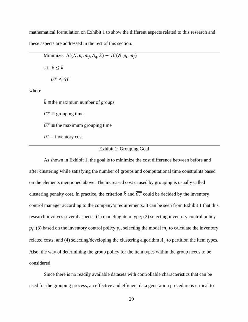
29

mathematical formulation on Exhibit 1 to show the different aspects related to this research and

these aspects are addressed in the rest of this section.

Minimize: 𝐼𝐼(𝑁, 𝑝𝑖,𝑚𝑗 ,𝐴𝑞, 𝑘) − 𝐼𝐼(𝑁,𝑝𝑖 ,𝑚𝑗)

s.t.: 𝑘 ≤ 𝑘�

𝐺𝐺 ≤ 𝐺𝐺����

where

𝑘� ≡the maximum number of groups

𝐺𝐺 ≡ grouping time

𝐺𝐺���� ≡ the maximum grouping time

𝐼𝐼 ≡ inventory cost

Exhibit 1: Grouping Goal

As shown in Exhibit 1, the goal is to minimize the cost difference between before and

after clustering while satisfying the number of groups and computational time constraints based

on the elements mentioned above. The increased cost caused by grouping is usually called

clustering penalty cost. In practice, the criterion 𝑘� and 𝐺𝐺���� could be decided by the inventory

control manager according to the company’s requirements. It can be seen from Exhibit 1 that this

research involves several aspects: (1) modeling item type; (2) selecting inventory control policy

𝑝𝑖; (3) based on the inventory control policy 𝑝𝑖, selecting the model 𝑚𝑗 to calculate the inventory

related costs; and (4) selecting/developing the clustering algorithm 𝐴𝑞 to partition the item types.

Also, the way of determining the group policy for the item types within the group needs to be

considered.

Since there is no readily available datasets with controllable characteristics that can be

used for the grouping process, an effective and efficient data generation procedure is critical to

30

provide the data for grouping. Before designing the data generation procedure, how the system

can be represented as data that can be clustered should be determined through data modeling

techniques.

Further, the quality of the grouping results need to be tested from statistical and

optimization perspectives. Since there is no exact control policy optimization technique available

for the multi-echelon inventory system described in this research, the heuristic procedure for

setting the optimal inventory control parameters at single location developed in Hadley and

Whitin (1963) is extended to the multi-echelon case. This approach is called Extended Hadley

and Whitin Solution (EHWS). The main purpose of this optimization technique is to provide a

way to relatively compare different grouping methods developed in this dissertation.

It can be seen from the discussions above that the whole research process is an

integration of data modeling, data generation, grouping, and optimization procedure as shown in

Figure 2.

Figure 2: Research Process

The relationships among the elements in Figure 3 are summarized as follows:

1) The system and item characteristics and their relationships are quantified using data

modeling; as a result, data models are developed.

2) Data generation methods are developed based on the data models to provide large

scale datasets for grouping.

31

3) The grouping methods are selected for different system and item characteristics.

4) The data that represents the system and item is clustered using grouping methods

accordingly.

5) The clusters resulting from the clustering process are evaluated from statistical

analysis and optimization perspectives.

6) The grouping evaluation process identifies the attributes that have significant impact

on the clustering results. These attributes should be included in the system characteristics.

The key issues regarding the inventory control policy, inventory control models,

grouping techniques applied in this research are discussed in Section 3.1, 3.2, and 3.3

respectively. The data modeling and data generation are discussed in Chapter 4.

3.1 Inventory Control Policy

The main policies that are typically used in inventory control practice are (1) order point,

order quantity policy (R, Q); (2) order point, order up to level policy (R, S); (3) periodic review,

order up to level policy (s, S); and (4) (R, s, S) policy which is a combination of (R, S) and (s, S)

policies.

The reorder point reorder quantity policy ((r, Q) policy) is selected in this research for the

following reasons: (1) it is easy to implemented and widely used in the industry; (2) it is a

common practice to compute order quantity Q and reorder point r separately (Hopp et al. 1997),

and (3) calculating reorder points and order quantities separately does not result in large errors

(Zhang, Hopp and Supatgiat 2001; Zheng 1992).

3.2 Inventory Control Model

In this sub-section, the four inventory cost models from the literature are compared and

the most appropriate one is selected and extended to solve the multi-echelon problem of interest

32

in this research. Some of these models are also used to derive the rules to build the classification

criterion in section 3.3.1. For the comparison and review convenience, they are listed as follows:

Model 1: Zhang, Hopp and Supatgiat’s Model

Zhang et al. (2001) formulate the inventory control problem as minimizing inventory

investment subjecting to constraints on average service level and replenishment frequency. The

model is as follows:

Minimize: ∑ 𝑐𝑖 �𝑟𝑖 − 𝜃𝑖 + 𝑄𝑖2

+ 12

+ 𝐵𝑖(𝑟𝑖 ,𝑄𝑖)�𝑁𝑖=1

s.t. 1𝑁∑ 𝐷𝑖

𝑄𝑖𝑁𝑖=1 ≤ 𝐹

∑ 𝐷𝑖𝐷𝑡𝑡𝑡

(1 − 𝐴𝑖(𝑟𝑖 ,𝑄𝑖))𝑁𝑖=1 ≥ S

𝑟𝑖 ≥ 𝑟𝑖

𝑄𝑖 ≥ 1

𝑟𝑖 ,𝑄𝑖: 𝑖𝑛𝑖𝑖𝑖𝑖𝑟𝑖

Where

𝑁 ≡ number of items

𝑐𝑖 ≡ unit cost for item 𝑖

𝐷𝑖 ≡ expected demand for item 𝑖 per year

𝐷𝑡𝑡𝑡 ≡ ∑ 𝐷𝑖𝑁𝑖=1

𝑙𝑖 ≡ replenishment leadtime for item 𝑖

𝜃𝑖 ≡ 𝐷𝑖𝑙𝑖 , expected demand for item 𝑖 𝑑𝑑𝑟𝑖𝑛𝑖 𝑙𝑖𝑙𝑑 𝑖𝑖𝑚𝑖 𝑙𝑖

𝜎𝑖 ≡ standard deviation of demand during lead time for item 𝑖

𝑄𝑖 ≡ order quantity for item 𝑖

𝑟𝑖 ≡ reorder point for item 𝑖

33

𝑟𝑖 ≡ preset value for reorder point of the item 𝑖

𝐴𝑖(𝑟𝑖 ,𝑄𝑖) ≡ probability of stockout for item 𝑖

𝐵𝑖(𝑟𝑖 ,𝑄𝑖) ≡ expected number of backorders for item 𝑖 at any time

Exhibit 2: Zhang, Hopp and Supatgiat’s Detailed Model

Model 2: Teunter, Babai and Syntetos’s Model

Teunter et al. (2010) develop a model to minimize total inventory cost while satisfying

the constraint on average fill rate over all SKUs. The model is as follows:

Minimize: ∑ �ℎ𝑖𝑆𝑆𝑖 − ℎ𝑖𝑄𝑖2

+ 𝑏𝑖𝐷𝑖(1 − 𝐹𝑅𝑖)�𝑁𝑖=1

Where

𝑁 ≡ number of SKUs

𝑏𝑖 ≡ penalty cost for SKU 𝑖

𝐼𝑆𝐶𝑖 ≡ 1 − ℎ𝑖𝑄𝑖𝑏𝑖𝐷𝑖

, cycle service level for SKU 𝑖

𝐷𝑖 ≡ demand per unit time for SKU 𝑖

𝐹𝑅𝑖 ≡ fill rate for SKU 𝑖

ℎ𝑖 ≡ inventory holding cost for SKU 𝑖

𝐶𝑖 ≡ lead time for SKU 𝑖

𝑄𝑖 ≡ (average) order quantity for SKU 𝑖

𝑆𝑆𝑖 ≡ safety stock for SKU 𝑖

Exhibit 3: Teunter, Babai and Syntetos’s Model

Model 3: Hopp and Spearman’s Model

Hopp and Spearman (2001) develop a model to minimize the inventory related cost

subjecting to order frequency and back order constraints. The model is as follows:

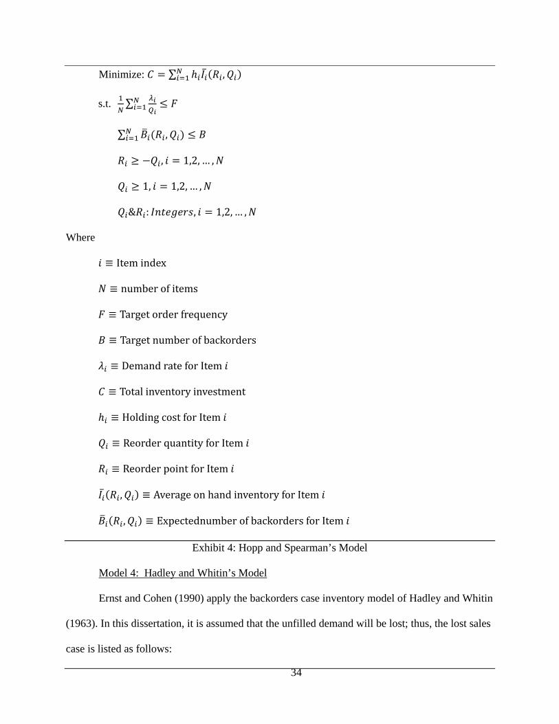
34

Minimize: 𝐼 = ∑ ℎ𝑖𝐼�̅�(𝑅𝑖 ,𝑄𝑖)𝑁𝑖=1

s.t. 1𝑁∑ 𝜆𝑖

𝑄𝑖𝑁𝑖=1 ≤ 𝐹

∑ 𝐵�𝑖(𝑅𝑖 ,𝑄𝑖)𝑁𝑖=1 ≤ 𝐵

𝑅𝑖 ≥ −𝑄𝑖 , 𝑖 = 1,2, … ,𝑁

𝑄𝑖 ≥ 1, 𝑖 = 1,2, … ,𝑁

𝑄𝑖&𝑅𝑖: 𝐼𝑛𝑖𝑖𝑖𝑖𝑟𝑖, 𝑖 = 1,2, … ,𝑁

Where

𝑖 ≡ Item index

𝑁 ≡ number of items

𝐹 ≡ Target order frequency

𝐵 ≡ Target number of backorders

𝜆𝑖 ≡ Demand rate for Item 𝑖

𝐼 ≡ Total inventory investment

ℎ𝑖 ≡ Holding cost for Item 𝑖

𝑄𝑖 ≡ Reorder quantity for Item 𝑖

𝑅𝑖 ≡ Reorder point for Item 𝑖

𝐼�̅�(𝑅𝑖 ,𝑄𝑖) ≡ Average on hand inventory for Item 𝑖

𝐵�𝑖(𝑅𝑖 ,𝑄𝑖) ≡ Expectednumber of backorders for Item 𝑖

Exhibit 4: Hopp and Spearman’s Model

Model 4: Hadley and Whitin’s Model

Ernst and Cohen (1990) apply the backorders case inventory model of Hadley and Whitin

(1963). In this dissertation, it is assumed that the unfilled demand will be lost; thus, the lost sales

case is listed as follows:

35

Minimize: 𝐼(𝑟,𝑄) = 𝜆𝑄𝐴 + 𝐼𝐼 �𝑄

2+ 𝑟 − 𝜇𝐿𝐿� + �𝐼𝐼 + 𝑏𝜆

𝑄� �∫ (𝑥 − 𝑟)ℎ(𝑥)𝑑𝑥∞

𝑟 � （1）

Where

𝐴 ≡ ordering cost

𝑏 ≡ lost sales cost

𝐼 ≡ unit cost

𝜆 ≡ demand rate

𝐼 ≡ inventory holding charge

h(x) ≡ probability distribution of lead time demand assumed to be normal with

parameters (µLT,σLT)

Exhibit 5: Hadley and Whitin’s Model

All of these four inventory cost models are applied to evaluate performance of the

grouping algorithms by the authors. The 4th model, Hadley and Whitin’s Model, is used to

evaluate the performance of the grouping algorithms in this research for the following reasons: (1)

this research considers the importance-related attributes, i.e. shortage cost, during the ABC

classification process. Since Model 1 and Model 3 do not have importance-related attributes,

they are not suitable for this research; (2) for Model 2, the order quantity 𝑄𝑖 is derived based on

the historical data, and it is not optimized through the formulations. However, this dissertation

needs a model that can optimize reorder point and reorder quantity without referring to historic

data. Therefore, Model 4 is selected.

In Model 4, the shortage cost considered in this research is used to measure the criticality

of the items. The goal of Model 4 is to find optimal 𝑟∗ and 𝑄∗ to minimize the total cost. If

0 < 𝑄∗ < ∞, 0 < 𝑟∗ < ∞, then 𝑄∗ and 𝑟∗ satisfy 𝜕𝐼(𝑟,𝑄) 𝜕𝑄 =⁄ 0 and 𝜕𝐼(𝑟,𝑄) 𝜕𝑟 =⁄ 0. Thus,

following two equations can be derived.

36

𝑄 = �2𝜆[𝐴+𝑏∗𝜂(𝑟)]𝐼𝐼

（2）

𝐻(𝑟) = 𝑄𝐼𝐼

𝜆𝑏+𝑄𝐼𝐼 （3）

Where 𝜂(𝑟) ≡ ∫ (𝑥 − 𝑟)ℎ(𝑥)𝑑𝑥∞

𝑟

𝐻(𝑟) ≡ complementary cumulative of ℎ(𝑥)

If h(x) is a normal distribution, then the equivalent of (1) can be expressed as:

𝐼(𝑟,𝑄) = 𝜆𝑄𝐴 + 𝐼𝐼 �𝑄

2+ 𝑟 − 𝜇𝐿𝐿� + �𝐼𝐼 + 𝑏𝜆

𝑄� �(𝜇𝐿𝐿 − 𝑟)Φ�𝑟−𝜇𝐿𝐿

𝜎𝐿𝐿� + 𝜎𝐿𝐿𝜙(𝑟−𝜇𝐿𝐿

𝜎𝐿𝐿)� （4）

Where Φ(𝑥) ≡ cumulative distribution fucntion for 𝑥

𝜙(𝑥) ≡ probability density function for 𝑥

The approximate solution is obtained by applying the heuristic iterative procedure

developed in Section 4.4 of Hadley and Whitin (1963). The heuristic procedure can be

summarized as:

Step 1: Initialize 𝑄1 = �2𝐴𝜆𝐼𝐼

Step 2: Calculate 𝑟1 using equation (3) and Q1

Step 3: Calculate 𝑄2 using equation (2) and r1

Step 4: Calculate 𝑟2 using equation (3) and Q2

Step 5: If r2 is close to 𝑟1, then stop, 𝑟∗ = 𝑟2 and 𝑄∗ = 𝑄2; otherwise, let 𝑄1 = 𝑄2 and

𝑟1 = 𝑟2 and go back to Step 3.

Exhibit 6: Heuristic Procedure for Optimization

In order to apply Model 4 to the multi-echelon case in this research, several issues need

to be addressed: (a) determining of the mean and variance of lead time demand; (b) determining

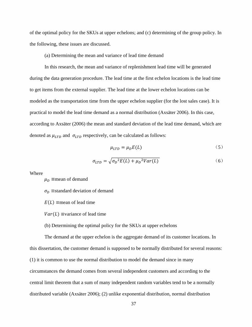
37

of the optimal policy for the SKUs at upper echelons; and (c) determining of the group policy. In

the following, these issues are discussed.

(a) Determining the mean and variance of lead time demand

In this research, the mean and variance of replenishment lead time will be generated

during the data generation procedure. The lead time at the first echelon locations is the lead time

to get items from the external supplier. The lead time at the lower echelon locations can be

modeled as the transportation time from the upper echelon supplier (for the lost sales case). It is

practical to model the lead time demand as a normal distribution (Axsäter 2006). In this case,

according to Axsäter (2006) the mean and standard deviation of the lead time demand, which are

denoted as 𝜇𝐿𝐿𝐷 and 𝜎𝐿𝐿𝐷 respectively, can be calculated as follows:

𝜇𝐿𝐿𝐷 = 𝜇𝐷𝐸(𝐶) （5）

𝜎𝐿𝐿𝐷 = �𝜎𝐷2𝐸(𝐶) + 𝜇𝐷2𝑉𝑙𝑟(𝐶) （6）

Where 𝜇𝐷 ≡mean of demand

𝜎𝐷 ≡standard deviation of demand

𝐸(𝐶) ≡mean of lead time

𝑉𝑙𝑟(𝐶) ≡variance of lead time

(b) Determining the optimal policy for the SKUs at upper echelons

The demand at the upper echelon is the aggregate demand of its customer locations. In

this dissertation, the customer demand is supposed to be normally distributed for several reasons:

(1) it is common to use the normal distribution to model the demand since in many

circumstances the demand comes from several independent customers and according to the

central limit theorem that a sum of many independent random variables tend to be a normally

distributed variable (Axsäter 2006); (2) unlike exponential distribution, normal distribution

38

allows the user to determine the mean and variance of the customer demand respectively; and (3)

the sum of two or more mutually independent normal random variables is still a normal random

variable. The property of normal random variables mentioned in the 3rd reason is one of the key

assumptions for the cost model in this research. Therefore, the mean and variance of the demand

at immediate upper echelon location can be expressed as in equation (7) and (8).

𝜇𝐷𝑢 = ∑ 𝜇𝐷(𝑖)𝑞

𝑖=1 （7）

where

𝜇𝐷𝑢 ≡ mean aggregate demand at the upper location

𝜇𝐷(𝑖) ≡ mean demand at the customer location i

𝑞 ≡ the number of customer locations

𝜎𝐷𝑢 = �∑ (𝜎𝐷(𝑖))2𝑞

𝑖=1 （8）

Where

𝜎𝐷𝑢 ≡ standard deviation of aggregate demand at the upper location

𝜎𝐷(𝑖) ≡ standard deviation of demand at the customer location i

𝑞 ≡ the number of customer locations

After the parameters of demand and lead time at the upper location are determined using

equations (7) and (8), the same heuristic procedure (Exhibit 6) described in Hadley and Whitin

(1963) is applied to calculate 𝑟∗ and 𝑄∗. A simple case is illustrated in Appendix 1, which

describes the procedures to set approximately optimal values of 𝑟∗ and 𝑄∗ for a single-item two-

echelon inventory system.

(c) Determining the group policy

39

For each item group, one inventory control policy is applied to items within the group.

For each item group, an aggregate item is built to represent the item group (Lenard and Roy

1995). The two main parameters of the aggregate item are the demand and lead time. Assume an

item family has p items, the mean and standard deviation of the aggregate demand can be

calculated as follows:

𝜇𝐷𝐴 = 1𝑝∑ 𝜇𝐷

(𝑖)𝑝𝑖=1 （9）

Where

𝜇𝐷𝐴 ≡mean of aggregate demand

𝜇𝐷(𝑖) ≡mean demand of item i within the group

𝜎𝐷𝐴 = �1𝑝∑ (𝜎𝐷

(𝑖))2𝑝𝑖=1 （10）

Where

𝜎𝐷𝐴 ≡standard deviation of aggregate demand

𝜎𝐷(𝑖) ≡standard deviation of the demand of item i within the group

Similarly, for the mean and standard deviation of the aggregate lead time can be

calculated as follows:

𝜇𝐿𝐿𝐴 = 1𝑝∑ 𝜇𝐿𝐿

(𝑖)𝑝𝑖=1 （11）

Where

𝜇𝐿𝐿𝐴 ≡mean lead time of aggregate item

𝜇𝐿𝐿(𝑖) ≡mean lead time of item i

𝜎𝐿𝐿𝐴 = �1𝑝∑ (𝜎𝐿𝐿

(𝑖))2𝑝𝑖=1 （12）

Where

40

𝜎𝐿𝐿𝐴 ≡standard deviation of the lead time of aggregate item

𝜎𝐿𝐿(𝑖) ≡standard deviation of the lead time of item i

After the parameters of demand and lead time are determined using equations (9)-(12),

the same procedure described in Hadley and Whitin (1963) is applied to calculate 𝑟∗ and 𝑄∗.

3.3 Grouping Techniques

This sub-section discusses the importance-based classification, the NIT classification,

and the operations-based clustering suggested in this research.

3.3.1 The ABC Classification

This research develops and evaluates an optimization model based on a single criterion

ABC classification technique, which groups items based on their importance. This single

criterion ABC classification technique is compared with other grouping techniques. This kind of

ABC classification technique avoids complex multi-criteria clustering methods and is proven to

be effective by Zhang et al. (2001) and Teunter et al. (2010). This section discusses the intuitions

of selecting appropriate ABC classification criterion by reviewing the two papers: Zhang et al.

(2001) and Teunter et al. (2010), summarizes the rule of selecting/developing classification

criterion, and develops the classification criterion for the network based ABC classification

technique.

The classification criterion for Zhang et al. (2001)

The inventory cost model in Zhang et al. (2001) is listed in Exhibit 2 (Model 1) in

Section 3.2. This model is to minimize inventory investment subject to constraints on average

service level and replenishment frequency. The authors suggest a categorization scheme based

on steps as follows:

41

a) Based on some approaches to the (r, Q) policy optimization problem in the literature,

the reorder point is expressed as:

𝑟𝑖 = 𝜃𝑖 + 𝑘𝑖𝜎𝑖

Where

𝜃𝑖 ≡ 𝐷𝑖𝑙𝑖 , expected demand for item 𝑖 during lead time 𝑙𝑖

𝜎𝑖 ≡ standard deviation of demand during lead time for item i

𝑟𝑖 ≡ reorder point for item i

b) Based on a single item model, given by the probability that there is no stockout during

lead time (Nahmias 1997), and using a service-constrained approach with Type I service 𝑆𝑖, the

𝑘𝑖 is decided as following:

𝑘𝑖 = 𝑧𝑆𝑖

Where

𝑧𝑆𝑖 ≡ the standard normal ordinate such that 𝛷�𝑧𝑆𝑖� = 𝑆𝑖

c) Based on the assumption that average inventory can be approximated by 𝑟𝑖 − 𝜃𝑖 + 𝑄𝑖2

and using Type I formula to compute average service level, the following expression for the

reorder point is derived (Hopp, Spearman and Zhang (1997)):

𝑘𝑖 = �−2𝑙𝑛 �√2𝜋�𝑙𝑖𝑐𝑖𝐷𝑡𝑡𝑡�𝐷𝑖𝜇

�

Where

𝑐𝑖 ≡ unit cost for item i

𝑙𝑖 ≡ replenishment lead time for item i

𝜇 ≡ the Lagrange multiplier corresponding to the average service constraint

𝐷𝑖 ≡ expected demand for item i per year

42

𝐷𝑡𝑡𝑡 ≡ ∑ 𝐷𝑖𝑁𝑖=1

d) The expression of 𝑘𝑖 suggests that items with higher values of 𝐷𝑖𝑙𝑖𝑐𝑖

2 result in higher 𝑘𝑖

values; therefore, higher service level is obtained for the given values of 𝐷𝑖, 𝑙𝑖, and 𝑐𝑖. Thus, 𝐷𝑖𝑙𝑖𝑐𝑖

2

was used by Zhang et al. (2001) as a classification criterion.

The classification criterion for Teunter et al. (2010)

The inventory cost model in Teunter et al. (2010) is listed in Exhibit 3 (Model 2) in

Section 3.2. Model 2 is to minimize total inventory cost with the constraint on average fill rate

over all SKUs. The authors propose a classification criterion based on the observation of cycle

service level for SKU (𝐼𝑆𝐶𝑖). Minimizing the total cost results in the following approximate

newsboy-type optimality condition:

𝐼𝑆𝐶𝑖 ≡ 1 −ℎ𝑖𝑄𝑖𝑏𝑖𝐷𝑖

Where

𝑏𝑖 ≡ penalty cost for SKU i

ℎ𝑖 ≡inventory holding cost for SKU i

𝐷𝑖 ≡demand per unit time for SKU i

𝑄𝑖 ≡(average) order quantity for SKU i

This condition indicates that the service level for a SKU is increasing with the increment

of the ratio 𝑏𝑖𝐷𝑖ℎ𝑖𝑄𝑖

. Therefore, the ratio 𝑏𝑖𝐷𝑖ℎ𝑖𝑄𝑖

is chosen as the classification criterion and the SKUs are

ranked based on the ratio in descending order.

From the analysis of development of classification criterion in Zhang et al. (2001) and

Teunter et al. (2010), it can be seen that the selection of classification criterion follows several

rules:

43

1) The selection of classification criterion is model specific.

2) The classification criterion reflects the inventory management goal.

3) The item with higher value of the classification criterion is more important.

Extending rule 2) to the management of multi-item multi-echelon inventory system of

interest leads to following rule:

4) The classification criterion should reflect the inventory network management goal.

These classification criterion selection rules are applied in this research. As discussed in

Section 3.1, Hadley and Whitin’s Model (Model 4 listed in Exhibit 5) is selected in this research,

and a network inventory cost criterion that affects the system performance is developed based on

this model. For an inventory system with more than one location, the cost function for the entire

network of one item is the sum of the cost related to each location j. For one location, the

inventory related cost is the sum of ordering cost (𝑂𝐼𝑗), average annual inventory holding cost

(𝐼𝐻𝐼𝑗) and the lost sale cost (𝐶𝑆𝐼𝑗). The expressions of aforementioned three components are

illustrated in equations (13) to (15).

𝑂𝐼𝑗 = 𝜆𝑗𝑄𝐿𝑗

𝐴𝑗 （13）

Where

𝑂𝐼𝑗 ≡ordering cost at location j

𝜆𝑗 ≡ demand rate at location j

𝑄𝐿𝑗 ≡ reorder quantity at location j

𝐴𝑗 ≡ ordering cost per time at location j

𝐼𝐻𝐼𝑗 = 𝐼𝑗𝐼 �𝑄𝐿𝑗2

+ 𝑟𝐿𝑗 − 𝜇𝐿𝐿_𝑗� + 𝐼𝑗𝐼 �∫ 𝑥ℎ(𝑥)𝑑𝑥 − 𝑟𝐿𝑗𝐻(𝑟𝐿𝑗)∞

𝑟𝐿𝑗� （14）

Where

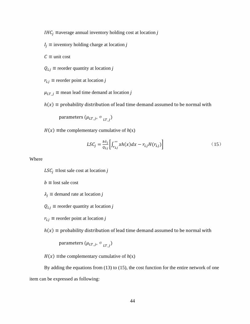
44

𝐼𝐻𝐼𝑗 ≡average annual inventory holding cost at location j

𝐼𝑗 ≡ inventory holding charge at location j

𝐼 ≡ unit cost

𝑄𝐿𝑗 ≡ reorder quantity at location j

𝑟𝐿𝑗 ≡ reorder point at location j

𝜇𝐿𝐿_𝑗 ≡ mean lead time demand at location j

ℎ(𝑥) ≡ probability distribution of lead time demand assumed to be normal with

parameters (𝜇𝐿𝐿_𝑗 ,σ𝐿𝐿_𝑗)

𝐻(𝑥) ≡the complementary cumulative of h(x)

𝐶𝑆𝐼𝑗 = 𝑏𝜆𝑗𝑄𝐿𝑗

�∫ 𝑥ℎ(𝑥)𝑑𝑥 − 𝑟𝐿𝑗𝐻(𝑟𝐿𝑗)∞

𝑟𝐿𝑗� （15）

Where

𝐶𝑆𝐼𝑗 ≡lost sale cost at location j

𝑏 ≡ lost sale cost

𝜆𝑗 ≡ demand rate at location j

𝑄𝐿𝑗 ≡ reorder quantity at location j

𝑟𝐿𝑗 ≡ reorder point at location j

ℎ(𝑥) ≡ probability distribution of lead time demand assumed to be normal with

parameters (𝜇𝐿𝐿_𝑗 ,σ𝐿𝐿_𝑗)

𝐻(𝑥) ≡the complementary cumulative of h(x)

By adding the equations from (13) to (15), the cost function for the entire network of one

item can be expressed as following:

45

∑ � 𝜆𝑗𝑄𝐿𝑗

𝐴𝑗 + 𝐼𝑗𝐼 �𝑄𝐿𝑗2

+ 𝑟𝐿𝑗 − 𝜇𝐿𝐿_𝑗� + �𝐼𝑗𝐼 + 𝑏𝜆𝑗𝑄𝐿𝑗� �∫ 𝑥ℎ(𝑥)𝑑𝑥 − 𝑟𝐿𝑗𝐻(𝑟𝐿𝑗)∞

𝑟𝐿𝑗��𝑁𝐿

𝑗=1 (16)

Where

𝑁𝐶 ≡ number of locations that hold inventory

𝐼 ≡ unit cost

𝑏 ≡ lost sales cost

𝐴𝑗 ≡ ordering cost per time at location j

𝐼𝑗 ≡ inventory holding charge at location j

𝜆𝑗 ≡ demand rate at location j

𝜇𝐿𝐿_𝑗 ≡ mean lead time demand at location j

𝜎𝐿𝐿_𝑗 ≡ standard deviation of lead time demand at location j

𝑟𝐿𝑗 ≡ reorder point at location j

𝑄𝐿𝑗 ≡ reorder quantity at location j

ℎ(𝑥) ≡ probability distribution of lead time demand assumed to be normal with

parameters (𝜇𝐿𝐿_𝑗 ,σ𝐿𝐿_𝑗)

𝐻(𝑥) ≡the complementary cumulative of h(x)

Since ℎ(𝑥) is assumed to be a normal distribution, the cost function (16) for the entire

network can be further expressed as following:

∑ �

𝜆𝑗𝑄𝐿𝑗

𝐴𝑗 + 𝐼𝑗𝐼 �𝑄𝐿𝑗2

+ 𝑟𝐿𝑗 − 𝜇𝐿𝐿_𝑗�

+ �𝐼𝑗𝐼 + 𝑏𝜆𝑗𝑄𝐿𝑗� ��𝜇𝐿𝐿_𝑗 − 𝑟𝐿𝑗�𝛷 �

𝑟𝐿𝑗−𝜇𝐿𝐿_𝑗

𝜎𝐿𝐿_𝑗� + 𝜎𝐿𝐿_𝑗𝜙(𝑟𝐿𝑗−𝜇𝐿𝐿_𝑗

𝜎𝐿𝐿_𝑗)��𝑁𝐿

𝑗=1 (17)

Where

𝑁𝐶 ≡ number of locations that hold inventory

𝐼 ≡ unit cost

46

𝑏 ≡ lost sales cost

𝐴𝑗 ≡ ordering cost per time at location j

𝐼𝑗 ≡ inventory holding charge at location j

𝜆𝑗 ≡ demand rate at location j

𝜇𝐿𝐿_𝑗 ≡ mean lead time demand at location j

𝜎𝐿𝐿_𝑗 ≡ standard deviation of lead time demand at location j

𝑟𝐿𝑗 ≡ reorder point at location j

𝑄𝐿𝑗 ≡ reorder quantity at location j

𝛷(𝑥) ≡ cumulative distribution function for x

𝜙(𝑥) ≡ probability density function for x

The total network inventory cost (NIC) in Equation (17) is selected as the network

classification criterion since: 1) it is directly from the cost model; 2) it reflects the inventory cost

management goal; 3) the higher value of NIC means the item is more important; and 4) it is the

total network cost which represents the network management goal.

The procedure to implement the importance-based classification from the network

perspective is summarized as follows:

Step 1: For each item i, calculate the network cost 𝑁𝐼𝐼𝑖.

Step 2: Sort items according to 𝑁𝐼𝐼𝑖. in descending order.

Step 3: Partition the items into three classes A, B, and C. The A class contain about 20%

of the top items, the B class contain about next 30% items and the C class contain the rest of

50% items.

Exhibit 7: The Procedures for Importance-Based Classification using 3 groups

47

3.3.2 The NIT Classification

As discussed in Section 2.2.3, the NIT classification depends on the representation of

NIT. It should be noted that the NIT representation is part of the interest of exploring the best

ways to represent the system in a mathematical and computer data structure format to facilitate

the analysis of the system and implementing the statistical grouping techniques. This section first

discusses two NIT expressions, from graph theory and binary perspectives, and then selects the

most appropriate NIT expression to implement NIT classification.

The NIT modeling is based on the following NIT related assumptions:

1) Each customer location has only one supplier in an NIT.

2) Each IHP is supplied by an IHP that is located at the immediate higher echelon,

except those IHPs located at the first echelon, which are supplied by the external suppler.

3) Each NIT has at least one retail store.

4) End customer demands are satisfied by the retail locations which are the lowest

echelon IHPs.

5) Each location is located at only one echelon.

Exhibit 8: The characteristics of NIT

In the following, the NIT modeling is discussed from graph theory expression and binary

expression perspectives respectively.

Graph Theory Expression

The inventory network system (and the structural attribute NIT) can be expressed as a

tree using graph theory as in Figure 3. A tree is a graph that does not include any simple circuits,

which means it has no loops and no more than one edge between any two different vertices. In

Figure 3, the external supplier is represented as the root of the tree, and the retail stores are

48

represented as the leaves of the tree. The supplier locations are deemed as the parent nodes of

their customer locations, which are deemed as the child nodes of their parent nodes. Further, the

supplier-customer relations are represented by the edge that connecting the supplier and

customer locations.

Figure 3: The representation the location network

Based on the graph representation of the inventory system, a NIT can be represented as

Tree (V, E) or T (V, E), where the V is a set of vertices representing the corresponding nodes,

and the E represents a set of edges that connecting two vectors. For example, the tree in Figure 3

can be represented as T(V, E), where V={1,2,3,4,5,6,7}, and E = {(1,2),(1,3),(2,4),(2,5),(3,6),

(3,7)}.

The corresponding relations between the system components discussed in Section 1 and

the components in the Tree are summarized as in Table 2.

Table 2: The Components of the Inventory system and the Tree

Components of the Inventory system

External Supplier

Retailer Stores

Supplier Location

Customer Location

Supplier-Customer Relation

Components of the Tree

Root Leaf Parent node Child node Edge

The tree representing a NIT has the characteristics such as: (1) it is a connected graph

with n vertices and n−1 edges, where n is any positive integer; (2) it has no loops and no more

49

than one edge between any two different vertices; in other words, there is a unique simple path

between any two of its vertices; (3) it is a rooted tree in which the vertex representing the

External Supplier is designated as the root and every edge is directed away from the root. In the

rest of this research, the term NIT is equivalent to Tree.

It can be noted that these characteristics are consistent with the inventory location

network structure related assumptions described in Section 1. In the inventory system of interest,

for each item type, each IHP is supplied by an IHP that is located at the immediate higher

echelon, except those IHPs located at the first echelon, which are supplied by the external

suppler. This is consistent with the characteristic (2) mentioned above. The items for the

inventory system are supplied by the External Supplier, which is represented as the root of the

NIT tree, and the supplying direction of these items are directed away from this root. This

corresponds to the NIT tree characteristic (3).

Based on the NITs represented in graphs, the relations between the NITs can be specified.

Suppose there are two trees 𝑁𝐼𝐺1(𝑉1,𝐸1) and 𝑁𝐼𝐺2(𝑉2,𝐸2). The following relations can be

specified:

• Definition 1: 𝑁𝐼𝐺1 is a sub-graph of 𝑁𝐼𝐺2, if 𝑉1 ⊆ 𝑉2and 𝐸1 ⊆ 𝐸2

• Definition 2: The 𝑁𝐼𝐺1is equal to 𝑁𝐼𝐺2, if 𝑁𝐼𝐺1 is a sub-graph of 𝑁𝐼𝐺2 and 𝑁𝐼𝐺2 is a

sub-graph of 𝑁𝐼𝐺1.

• Definition 3: 𝑁𝐼𝐺1 and 𝑁𝐼𝐺2 are partly same if 𝑁𝐼𝐺1 is not a sub-graph of 𝑁𝐼𝐺2, 𝑁𝐼𝐺2 is

not a sub-graph of 𝑁𝐼𝐺1, and the union of 𝑁𝐼𝐺1and 𝑁𝐼𝐺2 (𝑁𝐼𝐺1 ∪ 𝑁𝐼𝐺2) is a Tree.

• Definition 4: 𝑁𝐼𝐺1 and 𝑁𝐼𝐺2 are different if the union of 𝑁𝐼𝐺1and 𝑁𝐼𝐺2 (𝑁𝐼𝐺1 ∪ 𝑁𝐼𝐺2) is

not a Tree.

50

Based on these four definitions, the relations (similarities) of the NITs can be

summarized as: (1) equal; (2) sub graph; (3) partly same; (4) different.

In order to compare two NITs base on the graph representation, all vertices and edges of

two NITs should be compared.

Binary Expression

The existence of each location can be expressed by a binary value where “1” indicates the

existence of the corresponding location for the item and “0” means the non-existence. This

means that the NIT can be expressed as a number of binary values, each of which represents the

existence of a location. Based on this idea, the NIT illustrated in Figure 3 can be represented

using Table 3:

Table 3: Binary Expression of NIT Based on All Locations

L1 L2 L3 L4 L5 L6 L7 1 1 1 1 1 1 1

The characteristics of the NIT listed in Exhibit 8 indicate that the structure of a NIT can

be determined by the retail stores located at the lowest echelon. This means that the binary

expression of the NIT in Table 3 can be represented using only the binary values for retail stores.

Therefore, the ultimate resulted binary expression for NIT can be expressed as in Table 4. From

now on in this dissertation, the binary expression for NIT refers to binary expression for NIT

based on retail stores.

Table 4: Binary Expression for NIT Based on Retail Stores

L1 L2 L3 L4 1 1 1 1

51

Based on the binary expression for NIT, the comparison between two NITs can be

reduced to comparing the structure of lowest echelon. The process of determining whether two

NITs, for example 𝑁𝐼𝐺1 and 𝑁𝐼𝐺2, are the same can be realized by checking whether each retail

store in 𝑁𝐼𝐺1 exists in 𝑁𝐼𝐺2 and whether each retail store in 𝑁𝐼𝐺2 exists in 𝑁𝐼𝐺1. If there is any

retail store in 𝑁𝐼𝐺1 that does not exist in 𝑁𝐼𝐺2 or any retail store in 𝑁𝐼𝐺2 that does not exist in

𝑁𝐼𝐺1, then 𝑁𝐼𝐺1 and 𝑁𝐼𝐺2 are different; otherwise, 𝑁𝐼𝐺1 and 𝑁𝐼𝐺2 are the same.

The binary expression of NIT is selected to classify the NITs in this research because of

following two reasons: 1) Lenard and Roy (1995) suggest that the storage structure is the

attribute on which differences between items prevent the grouping of the items. This is because

the function of the warehouse is different at different echelons, i.e., different warehouse has

different customers. This means that items with different NITs should be separated; 2) compared

to the graph theory expression, the binary expression of NIT is more efficient to determine

whether two NITs are the same.

The process to group items into NIT groups satisfying the condition that items within the

same NIT group have the same NIT structure is called NIT classification.

The NIT classification procedure can be summarized as follows:

1) Assign the first NIT to a new NIT group.

2) Iterate NITs from the second to the last. Compare each NIT with the first NIT in the

existing NIT group(s), if the current NIT is equal to the selected NIT, add it to the corresponding

group; otherwise create a new NIT group, and add the current NIT to it as the first NIT.

Exhibit 9: NIT Classification Procedure

52

3.3.3 The K-Means Clustering

It can be seen from the discussions that the clusters formed after classifying the item

types based on NITs would have two characteristics: (1) still include very large number of item

types; (2) the item characteristics values of some item types in a group are too different from

most of the remaining item types so that applying the same inventory control group policy for

these items is not reasonable. Thus, the item groups resulting only based on the NIT

classification may not satisfy the commonly held objective of grouping, which is “minimum

within-group variability and maximum between-group variability”, from the other item

characteristics perspectives, such as unit cost, demand rate, ordering cost, etc. This motivates the

further clustering these resulted groups into smaller groups based on the other most related

attributes.

This section discusses the K-Means Clustering from following perspectives: 1) selecting

clustering attributes based on whether they have an impact on the inventory management goal, 2)

specifying the distance measurement for the selected attributes, 3) based on the distance

measurement, introducing the K-Means clustering algorithm, 4) the technique to optimize the

number of clusters, and 5) a K-Means clustering method to cluster both structural and non-

structural attributes.

Since the Hadley and Whitin’s Model is selected in this research to calculate the

inventory cost, the variables in the model are used to cluster the items. These variables are unit

cost of item i (𝐼𝑖), lost sales cost of item i (𝑏𝑖), ordering cost of item i at location j (𝐴𝑖𝑗),

inventory holding charge of item i at location j (𝐼𝑖𝑗), demand rate of item i at retail store 𝑗𝑅 (𝜆𝑖𝑗𝑅),

standard deviation of demand of item i at retail store 𝑗𝑅 (𝜎𝐷_𝑖𝑗𝑅), mean lead time at location j for

item i (𝑀𝐶𝐺𝑖𝑗), variance of lead time at location j for item i (𝑉𝐶𝐺𝑖𝑗). In the rest of this dissertation,

53

the number of retail stores is denoted as NR, and the number of locations as NL. The distance

measures for the non-structural attributes are (2𝑁𝑅 + 4𝑁𝐶) dimensional squared Euclidean

distance for the following reasons:

1) One item has one unit cost and one lost sales penalty cost.

2) The mean and variance of demand at upper echelon location other than retail store

echelon can be derived based on 𝜆𝑖𝑗𝑅 and 𝜎𝐷_𝑖𝑗𝑅 at retail stores. Therefore, only the mean and

variance of demand at retail stores are considered as the clustering attributes.

3) The 𝑀𝐶𝐺𝑖𝑗 and 𝑉𝐶𝐺𝑖𝑗 may be different at different locations.

4) Except for the External Supplier, each location has an ordering cost and inventory

holding cost rate.

5) In sum, 2+2𝑁𝑅+2𝑁𝐶+2(𝑁𝐶 − 2)= 2𝑁𝑅 + 4𝑁𝐶 clustering attributes are obtained

based on the four reasons above.

Assume the location index is numbered continuously from 0 to (𝑁𝐶 − 1) with the

External Supplier as 0, and assume the retail stores are numbered through (𝑁𝐶 − 𝑁𝑅 − 1) to

(𝑁𝐶 − 1). The (2𝑁𝑅 + 4𝑁𝐶) dimensional space for the clustering attributes can be organized as

follows:

𝐴𝑖𝑖𝑟𝑖𝑏𝑑𝑖𝑖 𝐶𝑖𝑖𝑖 = (𝐼𝑖 , 𝑏𝑖 , 𝜆𝑖(𝑁𝐿−𝑁𝑅−1), … , 𝜆𝑖(𝑁𝐿−1),𝜎𝐷𝑖(𝑁𝐿−𝑁𝑅−1), … ,𝜎𝐷(𝑁𝐿−1) ,

𝐴𝑖1 … ,𝐴𝑖(𝑁𝐿−1), 𝐼𝑖1, … , 𝐼𝑖(𝑁𝐿−1),𝑀𝐶𝐺𝑖0, … ,𝑀𝐶𝐺𝑖(𝑁𝐿−1),𝑉𝐶𝐺𝑖0, … , 𝑉𝐶𝐺𝑖(𝑁𝐿−1))

Exhibit 10: Attribute List for Non-Structural Attributes

Using the attributes in Exhibit 10, the K-Means algorithm is selected in this research to

cluster the items since it is commonly used in practice to cluster large datasets. The commonly

used distance measure in K-Means algorithm is the Euclidean distance. The distance between

two items, 𝑋𝐴 and 𝑋𝐵, can be expressed as:

54

d(XA, XB) = dAB = �(CA′ − CB′ )2 + (bA′ − bB′ )2

+ � ��λAj′ − λBj′ �2 + �σDAj

′ − σDBj′ �

2�

NL−1

j=NL−NR−1

+ � ��MLTAj′ − MLTBj′ �2 + �VLTAj′ − VLTBj′ �

2�NL−1

j=0

+ � [(AA′ − AB

′ )2 + (IA′ − IB′ )2]NL−1

j=1�0.5

Where

𝐼𝑖′, 𝑏𝑖′, 𝜆𝑖𝑗′ ,𝜎𝐷𝑖𝑗′ ,𝑀𝐶𝐺𝑖𝑗′ ,𝑉𝐶𝐺𝑖𝑗′ ,𝐴𝑖′ , 𝐼𝑖′ are the normalized values.

Exhibit 11: Euclidean Distance

The normalized values for continuous-valued are obtained based on following formula:

𝑋𝑖′(𝑡) =

𝑋𝑖(𝑡) − min�𝑋𝑖

(𝑡)�

max�𝑋𝑖(𝑡)� − min�𝑋𝑖

(𝑡)�)

Where

𝑋𝑖(𝑡) ≡ t-th attribute of item i

𝑋𝑖′(𝑡) ≡ the normalized value of t-th attribute of item i

Exhibit 12: Normalization

Since all the clustering attributes in Exhibit 10 are continuous-valued, putting

normalization formulations into Exhibit 11, the Euclidean distance between two items can be

expressed as:

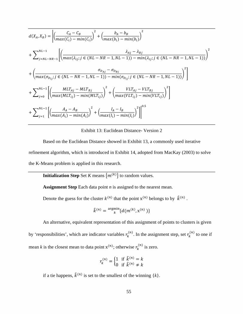
55

𝑑(𝑋𝐴,𝑋𝐵) = ��𝐼𝐴 − 𝐼𝐵

𝑚𝑙𝑥(𝐼𝑖) −𝑚𝑖𝑛(𝐼𝑖)�2

+ �𝑏𝐴 − 𝑏𝐵

𝑚𝑙𝑥(𝑏𝑖) −𝑚𝑖𝑛(𝑏𝑖)�2

+ � ��𝜆𝐴𝑗 − 𝜆𝐵𝑗

𝑚𝑙𝑥(𝜆𝑖𝑗; 𝑗 ∈ (𝑁𝐶 − 𝑁𝑅 − 1,𝑁𝐶 − 1)) −𝑚𝑖𝑛 (𝜆𝑖𝑗; 𝑗 ∈ (𝑁𝐶 − 𝑁𝑅 − 1,𝑁𝐶 − 1))�2𝑁𝐿−1

𝑗=𝑁𝐿−𝑁𝑅−1

+ �𝜎𝐷𝐴𝑗 − 𝜎𝐷𝐵𝑗

𝑚𝑙𝑥(𝜎𝐷𝑖𝑗; 𝑗 ∈ (𝑁𝐶 − 𝑁𝑅 − 1,𝑁𝐶 − 1)) −𝑚𝑖𝑛 (𝜎𝐷𝑖𝑗; 𝑗 ∈ (𝑁𝐶 − 𝑁𝑅 − 1,𝑁𝐶 − 1))�2

�

+ � ��𝑀𝐶𝐺𝐴𝑗 − 𝑀𝐶𝐺𝐵𝑗

𝑚𝑙𝑥(𝑀𝐶𝐺𝑖𝑗) −𝑚𝑖𝑛 (𝑀𝐶𝐺𝑖𝑗)�2

+ �𝑉𝐶𝐺𝐴𝑗 − 𝑉𝐶𝐺𝐵𝑗

𝑚𝑙𝑥(𝑉𝐶𝐺𝑖𝑗) −𝑚𝑖𝑛 (𝑉𝐶𝐺𝑖𝑗)�2

�𝑁𝐿−1

𝑗=0

+ � ��𝐴𝐴 − 𝐴𝐵

𝑚𝑙𝑥(𝐴𝑖) −𝑚𝑖𝑛 (𝐴𝑖)�2

+ �𝐼𝐴 − 𝐼𝐵

𝑚𝑙𝑥(𝐼𝑖) −𝑚𝑖𝑛 (𝐼𝑖)�2�

𝑁𝐿−1

𝑗=1�0.5

Exhibit 13: Euclidean Distance- Version 2

Based on the Euclidean Distance showed in Exhibit 13, a commonly used iterative

refinement algorithm, which is introduced in Exhibit 14, adopted from MacKay (2003) to solve

the K-Means problem is applied in this research.

Initialization Step Set K means �𝑚(𝑘)� to random values.

Assignment Step Each data point n is assigned to the nearest mean.

Denote the guess for the cluster 𝑘(𝑛) that the point x(𝑛) belongs to by 𝑘� (𝑛) .

𝑘� (𝑛) = {𝑑(𝑚(𝑘), x(𝑛) )}𝑘 argmin

An alternative, equivalent representation of this assignment of points to clusters is given

by ‘responsibilities’, which are indicator variables 𝑟𝑘(𝑛). In the assignment step, set 𝑟𝑘

(𝑛) to one if

mean k is the closest mean to data point x(𝑛); otherwise 𝑟𝑘(𝑛) is zero.

𝑟𝑘(𝑛) = �1 if 𝑘� (𝑛) = 𝑘

0 if 𝑘� (𝑛) ≠ 𝑘

if a tie happens, 𝑘� (𝑛) is set to the smallest of the winning {k}.

56

Update Step The model parameters, the means, are adjusted to match the sample means

of the data points that they are responsible for.

m(𝑘) =∑ 𝑟𝑘

(𝑛)𝑛

𝑅(𝑘)

where 𝑅(𝑘) is the total responsibility of mean k,

𝑅(𝑘) = �𝑟𝑘(𝑛)

𝑛

If 𝑅(𝑘) = 0, keep m(𝑘).

Repeat the assignment step and update step until the assignments do not change.

Exhibit 14: The K-Means Algorithm

The K-Means clustering algorithm requires the number of clusters K as an input

parameter. This parameter affects the performance of the clustering results significantly; thus, it

should be determined carefully. Tibshirani et al. (2001) develop a gap statistic approach to find

the optimal number of clusters based on the within-cluster scatter. Supposing the data {𝑥𝑖𝑗}, i=1,

2,…, n, j=1, 2,…, p, is composed of p dimensional space on n observations, supposing the

observations are partitioned in k clusters, 𝐼1, 𝐼2,…, 𝐼𝑘, and denoting 𝐼𝑟 as the indices of

observations in cluster r, Tibshirani et al. (2001) propose an error measure 𝑊𝑘, as following:

𝑊𝑘 = � �1

2𝑛𝑟� 𝑑𝑖𝑖′𝑖,𝑖′∈𝐼𝑟

�𝑘

𝑟=1

Where

𝑑𝑖𝑖′ ≡ The Euclidean distance between two observations i and 𝑖′

𝑛𝑟 ≡ The number of observations in k-th cluster

Exhibit 15: Error Measure

57

Their estimate of the optimal number of clusters is the value of k satisfying following

condition:

𝑀𝑙𝑥𝑖𝑚𝑖𝑧𝑖 𝐺𝑙𝑝𝑛(𝑘) = 𝐸𝑛∗{log(𝑊𝑘)} − log(𝑊𝑘)

Where

𝐸𝑛∗ ≡ The expectation under a sample of size n based on the reference distribution

Exhibit 16: Gap Statistic

The authors conclude that the uniform distribution is the most appropriate distribution to

perform a gap test. Considering partitioning n uniform data points in p dimensions with k centers,

and assuming that the centers are equally aligned, the expectation of log(𝑊𝑘) can be

approximately expressed as (Tibshirani et al. 2001):

log(𝑝𝑛 12⁄ ) − (2 𝑝⁄ ) log(𝑘) + 𝑐𝑐𝑛𝑖𝑖𝑙𝑛𝑖

Thus, using the uniform distribution as the reference distribution, the gap statistic can be

expressed as:

𝐺𝑙𝑝𝑛(𝑘) = log(𝑝𝑛 12⁄ ) − (2 𝑝⁄ ) log(𝑘) − log(𝑊𝑘) + 𝑐𝑐𝑛𝑖𝑖𝑙𝑛𝑖

Exhibit 17: Gap Statistic for Uniform Distribution

As shown, the last part of the expression in Exhibit 17 is a constant, which is independent

of n, p and k; thus, the constant can be ignored when comparing the value of Gap Statistic for

different k.

As discussed previously, the intuition behind the NIT classification is that structural

attributes (NIT in this research) prevents the grouping of items (Lenard and Roy 1995). The

relaxation of this assumption leads to another clustering method, i.e., clustering the items based

on both structural and non-structural attributes. The measurement for both structural and non-

structural attributes is the distance metrics for mixed-type attributes. Maimon and Rokach (2005)

58

suggest a way to calculate distance metrics for mixed-type attributes between two instances

using the Euclidean distance metric where the difference between binary attributes is calculated

as 0 or 1, and the difference between numeric attributes is calculated as the distance between

their normalized values. In this research, the non-structural attributes are numeric attributes and

the NIT attribute can be represented as a set of binary attributes, each of which represents the

existence of a location with the value 1 meaning “exist” and the value 0 meaning “not-exist”.

Therefore, the number of the clustering attributes for an item increases from (2𝑁𝑅 + 4𝑁𝐶) to

(3𝑁𝑅 + 4𝑁𝐶) where NR is the number of retail stores and 𝑁𝐶 is the number of locations. Among

the (3𝑁𝑅 + 4𝑁𝐶) clustering attributes, (2𝑁𝑅 + 4𝑁𝐶) clustering attributes are non-structural

attributes with numerical values, and 𝑁𝑅 clustering attributes are structural attributes with binary

values. The attribute list with both structural and non-structural attributes can be organized as

follows:

𝐴𝑖𝑖𝑟𝑖𝑏𝑑𝑖𝑖 𝐶𝑖𝑖𝑖

= (𝐸𝑖(𝑁𝐿−𝑁𝑅−1), … ,𝐸𝑖(𝑁𝐿−1),𝐼𝑖 , 𝑏𝑖 , 𝜆𝑖(𝑁𝐿−𝑁𝑅−1), … , 𝜆𝑖(𝑁𝐿−1),𝜎𝐷𝑖(𝑁𝐿−𝑁𝑅−1), … ,𝜎𝐷(𝑁𝐿−1),

𝐴𝑖1 … ,𝐴𝑖(𝑁𝐿−1), 𝐼𝑖1, … , 𝐼𝑖(𝑁𝐿−1),𝑀𝐶𝐺𝑖0, … ,𝑀𝐶𝐺𝑖(𝑁𝐿−1),𝑉𝐶𝐺𝑖0, … , 𝑉𝐶𝐺𝑖(𝑁𝐿−1))

Where

𝐸𝑖𝑗 ≡ the existence of location j for item i

𝐼𝑖 ≡ unit cost of item i

𝑏𝑖 ≡ lost sales cost of item i

𝜆𝑖𝑗 ≡ demand rate of item i at retail store j

𝜎𝐷(𝑖𝑗) ≡ standard deviation of demand of item i at retail store j

𝐴𝑖𝑗 ≡ ordering cost of item i at location j

𝐼𝑖𝑗 ≡ inventory holding charge item i at location j

59

𝑀𝐶𝐺𝑖𝑗 ≡ mean lead time at location j for item i

𝑉𝐶𝐺𝑖𝑗 ≡ variance of lead time at location j for item i

Exhibit 18: Attribute List for both Structural and Non-Structural Attributes

Maimon and Rokach (2005) define the dissimilarity 𝑑(𝑥𝑖 , 𝑥𝑗) between two instances

consisting of p attributes of mixed type as:

𝑑�𝑥𝑖 , 𝑥𝑗� =∑ 𝛿𝑖𝑗

(𝑛)𝑑𝑖𝑗(𝑛)𝑝

𝑛=1

∑ 𝛿𝑖𝑗(𝑛)𝑝

𝑛=1

Where

𝛿𝑖𝑗(𝑛) = 0 if one of the values is missing

If the attribute is binary, 𝑑(𝑛)�𝑥𝑖 , 𝑥𝑗� = 0 if 𝑥𝑖𝑛 = 𝑥𝑗𝑛; otherwise 𝑑(𝑛)�𝑥𝑖 , 𝑥𝑗� = 1

If the attribute is continuous-valued, 𝑑𝑖𝑗(𝑛) = � 𝑥𝑖𝑖− 𝑥𝑗𝑖�

𝑚𝑚𝑥ℎ𝑥ℎ𝑖−𝑚𝑖𝑛ℎ𝑥ℎ𝑖, where h runs over all non-

missing instances for n-th attribute.

Exhibit 19: Distance Metrics for Mixed-Type Attributes

Using the distance measures in Exhibit 19 and the aforementioned K-Means algorithm,

the items can be partitioned using both structural and non-structural attributes.

3.3.4 The categories of grouping techniques

The terms “Classification” and “Clustering” have similar meanings. Both of them refer to

cluster observations into smaller groups. However, the processes of classification and clustering

have some subtle differences. Their differences can be summarized into three perspectives: (1)

classification has determined labels before the grouping process, but clustering does not; (2)

while classification uses a clearly declared rule to group observations, clustering clusters

60

observations based on the distance measurement; (3) classification is one kind of supervised

process, but clustering is unsupervised process.

The ABC analysis and NIT grouping methods are categorized as classification techniques

and K-Means is a clustering technique. A summary of the comparison of ABC classification,

NIT classification, and K-Means clustering is illustrated in Table 5.

Table 5: Grouping Categories

Classification Clustering ABC NIT K-Means

Label Pre-determined A, B, C NIT1, NIT2,… None Grouping Method Pareto principle Same NIT structure Based on Euclidean distance

3.3.5 The Grouping Technique Evaluation

Bonner (1964) first argued that “there is no universal definition for what is a good

clustering”; the qualities of the clustering are determined based on the beholders experience. In

this dissertation, the clustering results are tested to quantitatively compare the clustering

techniques applied from both effectiveness (statistical and optimization) and efficiency (grouping

time) perspectives.

3.3.5.1 SSE as an Evaluation Criteria

From the statistical perspective, the compactness of the clusters is measured using Sum of

Squared Error (SSE). The SSE is chosen as the compactness measurement since it is the simplest

and most widely used criterion measure for clustering (Maimon and Rokach 2005). SSE can be

calculated as follows:

𝑆𝑆𝐸 = ����𝑥𝑖𝑗 − �̅�𝑗(𝑟)�

2𝑚

𝑗=1𝑖∈𝐼𝑟

𝑘

𝑟=1

Where k ≡ the number of clusters

61

m ≡ the number of dimensions of an observation

Cr ≡r-th centroid

x�j(r) ≡ the value of j-th dimension of r-th centroid

xij ≡ the value of j-th dimension of i-th observation

i ∈ Ci ≡ i-th observation in the group determined by i-th centroid

Exhibit 20: Sum of Squared Error

3.3.5.2 Penalty Cost as an Evaluation Criteria

From the optimization perspective, the Hadley and Whitin’s Model discussed in Section

3.2 is used to calculate the total inventory cost. The clustering penalty cost (CPC), which is the

increased cost caused by clustering, is used to measure the clustering effectiveness. The

clustering penalty cost can be expressed as following:

𝐼𝐶𝐼 = 𝐼𝐼(𝑁,𝑝,𝑚,𝐴𝑞,𝑘) − 𝐼𝐼(𝑁,𝑝,𝑚)

Where 𝐼𝐼 ≡ total inventory cost

𝑁 ≡ the set of item types

𝑝 ≡ inventory control policy, which is continuous (r, Q) policy

𝑚 ≡ inventory control model, which is Hadley and Whitin’s Model

𝐴𝑞 ≡ clustering algorithms q

𝑘 ≡ the number of clusters

Exhibit 21: Clustering Penalty Cost

It can be seen from Exhibit 21 that CPC is calculated by total cost after grouping, i.e.

𝐼𝐼(𝑁, 𝑝,𝑚,𝐴𝑞, 𝑘), minus total cost before grouping, i.e. 𝐼𝐼(𝑁,𝑝,𝑚). The total cost before

grouping is calculated based on following steps:

62

Step 1: for each item type in the system, optimize r and Q for each items as shown on

Exhibit 6. And then, using formula (17), which is defined based on p and m, the inventory cost

before grouping is calculated. Appendix 1 shows an example of calculating a single item’s total

cost.

Step 2: summing all item’s inventory cost before grouping results the total inventory cost

before grouping.

The difference between the calculation of before and after grouping total cost is that after

grouping total cost is calculated based on the group inventory policy. Based on selected 𝐴𝑞 and 𝑘,

items are grouped into different groups, and each group is treated as an aggregate item. The

aggregate item inventory policy related parameters are calculated based on formulas (9)-(12).

The total cost after grouping is calculated based on following steps:

Step 1: for each aggregate item in the system, optimize r and Q for each items as shown

on Exhibit 6.

Step 2: for each item, apply optimized r and Q from the corresponding aggregate item

(group) to calculate the total inventory cost using formula (17).

Step 3: sum all item’s inventory cost using group policy to obtain the total inventory cost

after grouping.

The %CPC measures the percent deviation with respect to the optimal individual

inventory policy. The value of %CPC shows the percent increase of total inventory cost when the

group policy is applied.

The %CPC is calculated using following equation:

63

%CPC =𝐺𝑐𝑖𝑙𝑙 𝐼𝑐𝑖𝑖 𝑙𝑎𝑖𝑖𝑟 𝑐𝑙𝑑𝑖𝑖𝑖𝑟𝑖𝑛𝑖 − 𝐺𝑐𝑖𝑙𝑙 𝐼𝑐𝑖𝑖 𝑏𝑖𝑎𝑐𝑟𝑖 𝑐𝑙𝑑𝑖𝑖𝑖𝑟𝑖𝑛𝑖

𝐺𝑐𝑖𝑙𝑙 𝐼𝑐𝑖𝑖 𝑏𝑖𝑎𝑐𝑟𝑖 𝑐𝑙𝑑𝑖𝑖𝑖𝑟𝑖𝑛𝑖

=𝐺𝑐𝑖𝑙𝑙 𝐼𝑐𝑖𝑖 𝑑𝑖𝑖𝑛𝑖 𝐺𝑟𝑐𝑑𝑝 𝐶𝑐𝑙𝑖𝑐𝑃 − 𝐺𝑐𝑖𝑙𝑙 𝐼𝑐𝑖𝑖 𝑑𝑖𝑖𝑛𝑖 𝐼𝑛𝑑𝑖𝐼𝑖𝑑𝑑𝑙𝑙 𝐶𝑐𝑙𝑖𝑐𝑃

𝐺𝑐𝑖𝑙𝑙 𝐼𝑐𝑖𝑖 𝑑𝑖𝑖𝑛𝑖 𝐼𝑛𝑑𝑖𝐼𝑖𝑑𝑑𝑙𝑙 𝐶𝑐𝑙𝑖𝑐𝑃

The %CPC is used to measure the effectiveness from the optimization perspective in the

rest of this dissertation.

3.3.5.3 The Grouping Time

From the efficiency perspective, the grouping time is used to assess the quality of

different grouping techniques. The lower the grouping time, the more efficient the grouping

technique. As discussed in Maimon and Rokach (2005), the time complexity of K-Means

algorithm relates to three attributes: 1) the number of instances (items); 2) the number of clusters;

and 3) the number of iterations used by the algorithm to converge. Besides these three attributes,

the number of clustering attributes is also an important factor affecting the clustering time, since

the more clustering attributes, the more computational memory is required to execute the

clustering. The effects of the aforementioned four factors on the grouping time of K-Means are

investigated in section 6.3. In addition, the comparisons of grouping time between different

grouping techniques are discussed in section 6.4.

64

4 Data Modeling and Generation

This Chapter first represents the system, item characteristics and their relations using data

modeling. Based on the data models created during the data modeling process, the data

generation procedures are discussed. The goal of data modeling and data generation discussed in

this chapter is to provide data for the research of grouping techniques.

4.1 Data Modeling

The characteristics of the inventory system of interest including the item characteristics

need to be represented in mathematical and computer data structure format to facilitate analysis

of the grouping methods. The data modeling process deals with the 1st research question

mentioned in the Introduction Chapter. The way to mathematically model structural attribute

NIT is discussed in section 3.3.2. This section explains the data modeling process applied in this

research from the computer data perspective.

The system of interest is made of large number of system elements that interact with each

other system wide. The item types in the inventory system are also the system elements, and they

interact with each other and with the other system elements as well. This means that quantifying

item type characteristics requires the quantification of other interacting elements with item types.

In brief, the quantification of the inventory system is to quantify the inventory system elements

and their relations. There are a variety of system element interactions, such as an item type can

be stored at specific locations, or an item type can be sold at certain locations, etc. To understand

the inventory system better, careful study of the interactions among system characteristics is

essential.

65

In the data modeling research, a top-down methodology is used to conduct the modeling

process, in which, the real world scenario is constructed first, and then the entities and

associations are identified. The steps of the data modeling process are as follows:

a) Summarizing the system characteristics

b) Building the E-R diagram

c) Mapping the E-R diagram to the relational model

Following, each step is summarized briefly.

4.1.1 Summarizing System Characteristics

The system characteristics involve a set of system element characteristics. The system

elements are identified based on the system description in Chapter 1, the optimization model

discussed in section 3.2, and the clustering attributes discussed in section 3.3. The identifying

system elements process basically is to identify the entities that independently exist in the system

and can be uniquely identified. These entities are item type, location, inventory policy, and

probability distribution. Based on these entities, the following section builds the related E-R

diagram.

4.1.2 Building the E-R Diagram

The E-R diagram is built through following steps: 1) identifying entities and drawing the

entity diagram; 2) identifying associations and drawing the association diagrams; and 3)

specifying the domain for each attribute. To illustrate the quantifiable aspects of the inventory

system of interest, such as relationships, behavior, structure etc., the UML diagram is employed

to draw the E-R diagram. A class is used to describe a group of objects with similar attributes,

common operations, common relationships to other objects, and common semantics (Rumbaugh

1991). In UML diagram, the notation for class and association are represented as shown in

66

Figure 4 and Figure 5 respectively. The multiplicity in Figure 5 specifies “the number of

instances of one class that may relate to a single instance of an associated class” (Rumbaugh

1991). The values for the multiplicity can be zero (0), one (1), or many (*). The multiplicity is

specified as [lower limit .. upper limit], where lower limit corresponds to the minimum

multiplicity and upper limit corresponds to maximum multiplicity. The notations in Figure 4 and

Figure 5 are used to draw the UML diagram for the entire inventory system.

Figure 4: UML Diagram Notation for Class

Figure 5: UML Diagram Notation for Association

The complete UML diagram of the inventory system is illustrated in Figure 6. The

detailed data modeling procedures are documented in Appendix 2, which includes the E-R

diagram, as shown on Figure 6, building process in details.

67

Figure 6: The E-R Diagram of the Inventory System

4.1.3 Mapping the E-R Diagram to the Relational Model

Based on the E-R diagram derived in the previous section, this section discusses how to

design the relational tables corresponding to the entity and association classes. The schema of the

tables is shown in the following format:

Table Name (Primary Key(s), Attribute 1, Attribute 2, … , Attribute N)

Normal forms are rules used to provide the guidance of designing tables. The tables

corresponding to the E-R diagram are built based on the third normal form. The tables are in

third normal form if they satisfy all the following criteria:

1) For each row, attributes must be atomic with only one value

2) Each non-primary key field is fully functional dependent on every key of the table

3) Each non-primary key field is non-transitively dependent on every key of the table

68

Exhibit 22: The Criteria for Third Normal Form

After mapping the UML diagram in Figure 6 to the relational models, there are six tables

resulted: Distribution, Location, Item Type, Demand Generator, SKU, and Shipment. The

detailed mapping process is described in Appendix 2.

4.1.4 Two Special Data Models

Based on the relational data models developed in the previous sections, this section

discusses two special data models: (1) Network of Item Type (NIT) and (2) Inventory System

(IS).

NIT data model contains two attributes: locations and the supply relation between

locations. The NIT for a specific item type can be derived using SKU table and Shipment table,

and an example is given in Appendix 2. When the ID of the item type is available, all the

locations of the corresponding item can be obtained from SKU table. Given the location IDs, the

related supply relation can be found in the Shipment table.

All the system elements are part of the Inventory System; thus, IS data model is an

aggregate of all the aforementioned data models.

The implementation of the data models in Java is recorded in Appendix 3.The next

section discusses the data generation procedure based on the data models developed in this

section.

4.2 Data Generation

This section discusses a method to generate large-scale datasets that represent the

inventory system and facilitate the testing of grouping methodologies. Based on the data models

designed in previous section, a data generation procedure was developed and used to generate

69

large-scale datasets. The basic goal of the data generation procedure is to generate a large scale

dataset including information of item types, locations, and SKUs, etc. To generate such a large

dataset, some automated procedure using programming tools such as Java, was needed to

conveniently and efficiently generate objects of SKUs holding both item type information and

location information.

This section is organized into four parts: 1) the relationships between data modeling and

data generation; 2) data generation procedure; 3) data quantification for inputs; and 4) data

generation evaluation.

4.2.1 Relationships between Data Modeling and Data Generation

The data modeling process determines the attributes of the objects contained in the

inventory system of interest and the relationships among the system objects. The connections

between data modeling and data generation can be summarized as follows:

1) The attributes of data models resulting from the data modeling process determine

what needs to be generated during the data generation process. The data generation

process generates new values and assigns the generated values to the attributes of the

data models.

2) The data modeling process determines the relations among the data models and some

relations are used to facilitate the data generation process. For example, each Item

Type model contains one Location Network data model. The SKUs, which are

determined by item type and locations, can be generated by iterating the locations in

the location network of the corresponding item type.

3) The data modeling process determines the structure of the storage files. After data

generation, the generated inventory system needs to be stored in files (such as CSV

70

files). During the clustering process, the information of the inventory system is read

from the files. The structures of the files are specified by the data models.

4.2.2 Data Generation Procedure

This section first discusses the generation of NIS and NIT, and then discusses the entire

data generation process.

4.2.2.1 NIS and NIT Generation

As discussed in Chapter 1, all the NITs combined form the network of inventory system

(NIS); this means that each NIT is a sub-network of the NIS. Both NIS and NIT are location

networks. During the data generation process, the NIS is first built; then, NIT for each item type

is built based on NIS and stored in the corresponding item type object.

Two kinds of inputs are needed to build the NIS: (1) the probability distribution for

number of echelons, and (2) the probability distribution(s) for number of customers for a supplier

location. The NIS building process follows the assumption that each customer location has only

one supplier location for item type. Figure 7 illustrates the process of building a three echelon

inventory system, in which there is 1 external supplier at echelon 0, 1 location at echelon 1, 2

locations at echelon 2, and 5 locations at echelon 3. The first step is to create a single External

Supplier. The following steps are to add locations from the highest echelon to the lowest. 𝑁𝐼𝑙

represents the number of customer locations for a supplier location l. As shown in Figure 7 (A),

where 𝑁𝐼0 = 1 means there is 1 customer location for the external supplier (with location ID 0),

adding locations starts from echelon 1 by putting 1 location at this echelon; on (B), where 𝑁𝐼1 =

2 means that there are 2 customer locations for location 1, 2 customer locations are assigned for

the location 1; on (C), 𝑁𝐼2=2 and 𝑁𝐼3=3 indicates there are 2 customer locations for location 2,

and 3 customer locations for location 2. Two customer locations are assigned to location 2 and

71

three customer locations are assigned to location 3 and this finishes the building of the entire

supply network.

Figure 7: Building the Supply Network

In reality, if an item type exists at a number of retail stores, which is located at the lowest

echelon, its entire supply network locations (or NIT) can be determined based on the assumption

that a customer location has only one supplier location for an item type. In the data generation

process, it is assumed that the item type’s existence at a retail store follows a probability

distribution. Based on this assumption, the lowest echelon IHPs are randomly determined

72

(generated). Once the retail stores having the item type are found, the item type’s supply network

can be decided; therefore the NIT is fixed as aforementioned.

Based on the supply network (NIS) built in Figure 7, Figure 8 illustrates the NIT building

process. Suppose an item type is stored at location 4, 5, 6, and 7, which are located at echelon 3

of the supply network as shown in Figure 8 (A). Since location 4 and 5 have single supplier

location 2, and location 6 and 7 has supplier location 3 as shown in Figure 7, the location 2 and 3

are decided as located at echelon 2 of the NIT as in Figure 8 (B). Further, since both locations 2

and 3 have single supplier 1, location 1 is determined as located at echelon 1 of the NIT as in

Figure 8 (C). Finally, since the External Supplier supplies the IHPs at echelon 1 and there is only

location 1 at the echelon, External Supplier is connected to location 1, and this finishes building

of the entire NIT as in Figure 8 (D). In sum, besides the two inputs needed to build the NIS (the

number of echelons, and number of customer locations for each supplier location), the NIT

building process requires one more input, i.e., the probability of item type’s existence at a

location located at the lowest echelon.

Figure 8: Building the Network of Item Type (NIT)

73

In reality, the number of retail stores is usually larger than the number of warehouses，

this indicates the number of customers at lower echelons is larger than the number of customers

at upper echelons. This characteristic of location networks can be achieved by applying a set of

uniform distributions satisfying the condition as following:

𝑈𝐵𝑒−1 ≤ 𝐶𝐵𝑒

Where

𝑈𝐵𝑒−1 ≡ upper bound of the number of customers for locations at echelon e-1

𝐶𝐵𝑒 ≡ lower bound of the number of customers for locations at echelon e

An example implementation of the mechanism above is illustrated in Table 6.

Table 6：Implementation of Uniform Distributions

Echelon Distribution for number of customers for a supplier location l (𝑁𝐼𝑙)

0 ~ Uniform(1, 2) 1 ~ Uniform(2, 3) 2 ~ Uniform(3, 5) … …

Another consideration about NIT is the lead time at IHPs. Usually, the lead time at the

lower echelons is shorter than that of upper echelons. This condition is satisfied using the

mechanism illustrated as follows:

(1) Generate the lead time at the External Supplier (LTatES).

(2) For the IHP other than the External Supplier, the lead time is set as the product of the

lead time of its supplier and a random variable from a Uniform (0.5, 1).

74

4.2.2.2 Summary of the Data Generation Procedure

This section presents the inputs and overview of the data generation procedure to create a

large-scale dataset that can quantitatively represent the multi-item multi-echelon inventory

system of interest.

The inputs of the data generation can be summarized as follows:

𝐷𝑁𝑁: The probability distribution for number of echelons

𝐷𝑁𝐼: The probability distribution for number of customers for a supplier location

𝐶𝐼: Probability of Item Type’s existence at a retail store (across any retailer location)

NI: Number of Item Types

𝐷𝑈𝐼: The probability distribution of item’s Unit Cost

𝐷𝐿𝑆𝐼: The probability distribution of item’s Lost-Sale-Cost-to-Unit-Cost Ratio

𝐷𝑂𝐼: The probability distribution of ordering cost

𝐷𝐻𝐼: The probability distribution of holding cost rate

𝐷𝐷𝑅: The probability distribution for demand rate

𝐷𝐷𝐷: The probability distribution for Demand Variance-to-Mean Ratio

𝐷𝐿𝐿𝑁𝑆: Lead Time distribution at External Supplier (day)

𝐷𝐿𝐿𝐼𝐻𝐿: Lead Time distribution at IHP (day)

𝐷𝐿𝐿𝐷: Lead Time Variance-to-Mean Ratio

The overview of data generation procedure can be summarized as in Figure 9. As shown,

the first step is to generate the physical network of inventory system (NIS), which holds the

entire inventory system. The second step is to generate the item types in the inventory system.

The third step deals with generating SKUs. The last step is to generate demands at the retailer

75

level. The rest of this section discusses the data generation procedure based on the inputs and the

aforementioned steps.

Generate NIS Generate Items Generate SKUs Generate Demand Parameters

Figure 9：Overview of data generation procedure

Step 1: Generating NIS

The number of echelons of the inventory system is randomly determined based on the

probability distribution 𝐷𝑁𝑁, which can be any discrete distribution; the discrete uniform

distributions is used in this research.

Once the number of echelons is determined, the physical inventory network system is

generated from top to bottom as discussed in 4.2.2.1. An example of a generated NIS is shown in

Figure 7 (C).

Step 2: Generating Items

This step first generates the structural attribute (NIT), and then generates the remaining

item attribute values for the corresponding items. The generation process of NIT is discussed in

4.2.2.1, and an example of generated NIT is given in Figure 8 (D). And then, the non-structural

attributes such as unit cost, lost sale cost, mean and variance of lead time at external supplier are

generated using distributions 𝐷𝑈𝐼, 𝐷𝐿𝑆𝐼, 𝐷𝐿𝐿𝑁𝑆, and 𝐷𝐿𝐿𝐷. All the items are generated by

repeating these two steps.

Step 3：Generating SKUs

Generation of SKUs for an item follows two steps. First, for an item type, iterate the

location information (location ID) sequentially in an NIT and combine this information with the

item type information (item type ID) stored at the corresponding location. This method forms

SKUs by combining item type ID and location ID automatically. This process is illustrated in

76

Figure 10. Second, for each SKU, ordering cost, inventory holding cost rate, and the mean and

variance of the Lead Time distribution between IHPs are generated using 𝐷𝑂𝐼, 𝐷𝐻𝐼 , 𝐷𝐿𝐿𝐼𝐻𝐿 and

𝐷𝐿𝐿𝐷. These two steps are repeated for all items.

Figure 10: SKU Generation Process

Step 4: Generating Demand Characteristics

Generation of demand for an item type also follows two steps. First, iterate all the SKUs

associated with the item, and create a demand generator for each SKU at the lowest echelon.

This process is illustrated on Figure 11. Second, for each Demand Generator, generate mean and

variance of demand rate using 𝐷𝐷𝑅 and 𝐷𝐷𝐷. These two steps are repeated for all item types.

Figure 11: Demand Generation Process

The pseudo code of the data generation procedure is recorded in Appendix 3.

4.2.3 Data Quantification for Inputs

Before the implementation of data generation, the values for input attributes and the

relationship between the attributes should be quantified. This section discusses these two issues.

77

4.2.3.1 The Range of Input Values

The input attributes are the ones that affect the system performance, for instance, total

inventory cost in this research. Based on the study of Chaharsooghi and Heydari (2010),

Deshpande et al. (2003), Ehrhardt (1984), Lee et al. (1997), Metters (1997), REM Associates,

and a case study from Tmall.com, the range of the input values are summarized in Table 7. The

detailed discussion about the data in Table 7 is in Appendix 4.

Table 7: Summary of Input Range

Attribute Range Reference Unit Cost ($) [1, 200,000] Deshpande et al. (2003) ,data from Tmall Lost-Sale-Cost-to-Unit-Cost Ratio [0.1,1] Metters (1997) Ordering Cost ($) [100,10000] Lee et al.(1997) Inventory Holding Charge ($/$/year) [12%,35%] REM Associates Demand Rate (yearly) [1,2000000] Deshpande et al. (2003), data from Tmall Demand Variance-to-Mean Ratio [0.1,4] Metters (1997), Lee et al.(1997) Mean lead time at ES (day) [10,250] Deshpande et al. (2003) Mean Lead Time at an IHP (day) [10,55] Deshpande et al. (2003) Lead Time Variance-to-Mean Ratio [0.01, 2]

Chaharsooghi and Heydari (2010), Ehrhardt (1984)

4.2.3.2 The Relationship between the Attributes

As mentioned in section 2.4, the motivation of generating data in this research is to

provide large-scale controllable datasets that closely reflect real inventory systems. This means

that, on the one hand, the large scale inventory dataset is not conveniently available from the

industry; on the other hand the real data from the industry cannot be manipulated to satisfy the

experimental needs in the research.

78

One of the important system characteristics in an inventory system is that some of the

system attributes interact with each other system wide, therefore their relations need to be closely

modeled to reflect the real world scenarios. Generally speaking, the generated data in this

research should have the characteristics such as 1) large scale; 2) the inputs can be controlled so

that different inventory systems can be generated according to the research objectives; 3) the

interactions (relationships) between the system characteristics should be closely modeled.

Keeping these perspective in mind, in the following data generation steps, first a set of data was

generated based on Rossetti and Achlerkar (2011), and then a regression analysis was

implemented to build three models reflecting the relationships between unit cost and lead time at

external supplier, ordering cost, and demand respectively.

Based on the literature and experience, some of the attribute relations in an inventory

system can be summarized as follows:

1) Average annual demand of an item is inversely proportional to its unit cost.

2) Average annual demand of an item is inversely proportional to the mean of its

replenishment lead time from External Supplier.

3) The ordering cost of an item is directly proportional to its unit cost.

4) The replenishment lead time of an item from External Supplier is directly proportional

to its unit cost.

Exhibit 23: The Assumptions about the Relationships between Attributes

The first two assumptions can also be found in Deshpande et al. (2003) and Rossetti and

Achlerkar (2011). The 3rd assumption is summarized based on experience. One of the reasons for

the high ordering cost for the items with high unit cost is that the shipping cost is more expensive

due to the higher insurance cost for more expensive items (the insurance cost is proportional to

79

the value of items in practice). In this research, the shipping cost is included in the ordering cost.

The 4th assumption is assumed based on the 1st and 2nd assumptions. In the real business world,

the fast-moving consumer goods have relatively low cost and high demand. The production

efficiency for these products is relatively high to meet the customer demands; thus, their

replenishment lead time is relatively short. The 1st and 3rd assumptions are also verified by the

regression analysis discussed in Appendix 4.

The mechanism to deal with relationships between attributes is developed based on

Rossetti and Achlerkar (2011). They use a sequence of conditional probability distributions to

randomly generate the attribute values. Their mechanism is illustrated using Table 8 (Adopted

from Rossetti and Achlerkar, (2011)).

Table 8: Attribute Values

% of Total Average Annual Demand Unit Cost Mean Lead Time

60% [100-500]H

[1000-10000]M-30% [5-20]M-30% [1-1000]L-60% [1-5]L-60% [10000-100000]H-10% [20-200]H-10%

30% [10-100]M

[10000-100000]H-30% [1-5]L-30% [1000-10000]M-60% [5-20]M-60% [1-1000]L-10% [20-200]H-10%

10% [0.5-10]L

[1-1000]L-30% [1-5]L-30% [10000-100000]H-60% [20-200]H-60% [1000-10000]M-10% [5-20]M-10%

The mechanism developed by Rossetti and Achlerkar (2011) follows several rules:

• Each attribute is associated with three uniform distributions: one for generating low

range values, one for generating medium range values, and one for generating high

range values. The ranges of these three distributions are continuous but not overlapped.

80

• The values of average annual demand are generated first, then, the values of other

attributes, such as unit cost and mean lead time, are generated based on their relations to

average annual demand.

• The generation of the value of average annual demand follows two steps: first, a discrete

probability distribution function is used to select the high, medium or low demand

category based on the discrete probabilities specified for each demand category. For

example, according to the “% of Total” column, the average annual demand has 60%

chance to be high category, 30% chance to be medium category, and 10% chance to be

low category; the second step is to generate the average annual demand value according

to the distribution specified for that category.

• The generation of attribute values other than average annual demand also follows two

steps. The generation of Mean Lead Time is described here as an example. The Mean

Lead Time also has three value distribution category, i.e., high, medium and low. First,

the chance of value category is determined by the direct or inverse relationship between

average annual demand and Mean Lead Time and by the value category of the average

annual demand. Suppose the values generated for average annual demand belongs to the

high category. Since the average annual demand of an item is inversely proportional to

the mean of its replenishment lead time, the low category value for Mean Lead Time has

more chance and high category has less chance. As a result, because the average annual

demand belongs to the high category, the value category for Mean Lead Time is

determined by the discrete probability distribution function with 10% for high category,

30% for medium category and 60% for low category; second, the values of the Mean

Lead Time is generated according to the distribution selected in the first step.

81

As mentioned previously, these data generation rules used in Rossetti and Achlerkar

(2011) are applied in this dissertation to deal with the relations between attributes mentioned in

Exhibit 23. Table 9 and Table 10 are the results of attribute values assignment according to the

mechanism proposed by Rossetti and Achlerkar (2011); these results satisfy the attribute

relationships in Exhibit 23. The corresponding range for High (H), Medium (M) and Low (L) is

specified in Table 11. The difference between their method and the method implemented in this

dissertation is that instead of generating average annual demand, this dissertation first generates

the values for unit cost, and then determine the attribute values for the other related attributes.

Table 9: Attribute Values for Assumption 1, 3 and 4

Unit Cost Ordering Cost Average Annual Demand Replenishment Lead Time

H H-60% H-10% H-60% M-30% M-30% M-30% L-10% L-60% L-10%

M H-20% H-20% H-20% M-60% M-60% M-60% L-20% L-20% L-20%

L H-10% H-60% H-10% M-30% M-30% M-30% L-60% L-10% L-60%

Table 10: Attribute Values for Assumption 2

Average Annual Demand Replenishment Lead Time

H H-10% M-30% L-60%

M H-30% M-60% L-10%

L H-60% M-30% L-10%

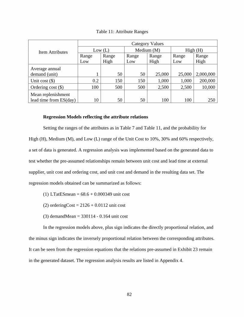
82

Table 11: Attribute Ranges

Item Attributes

Category Values Low (L) Medium (M) High (H)

Range Low

Range High

Range Low

Range High

Range Low

Range High

Average annual demand (unit) 1 50 50 25,000 25,000 2,000,000 Unit cost ($) 0.2 150 150 1,000 1,000 200,000 Ordering cost ($) 100 500 500 2,500 2,500 10,000 Mean replenishment lead time from ES(day) 10 50 50 100 100 250

Regression Models reflecting the attribute relations

Setting the ranges of the attributes as in Table 7 and Table 11, and the probability for

High (H), Medium (M), and Low (L) range of the Unit Cost to 10%, 30% and 60% respectively,

a set of data is generated. A regression analysis was implemented based on the generated data to

test whether the pre-assumed relationships remain between unit cost and lead time at external

supplier, unit cost and ordering cost, and unit cost and demand in the resulting data set. The

regression models obtained can be summarized as follows:

(1) LTatESmean = 68.6 + 0.000349 unit cost

(2) orderingCost = 2126 + 0.0112 unit cost

(3) demandMean = 330114 - 0.164 unit cost

In the regression models above, plus sign indicates the directly proportional relation, and

the minus sign indicates the inversely proportional relation between the corresponding attributes.

It can be seen from the regression equations that the relations pre-assumed in Exhibit 23 remain

in the generated dataset. The regression analysis results are listed in Appendix 4.

83

4.2.4 Data Generation Evaluation

In this dissertation, the effectiveness of the data generation methodology is measured by

the diversity of the data that represent the system of interest. A data generation process that

provides wide variety of inventory systems will facilitate the investigation of the large scale

multi item multi echelon inventory system characteristics. As discussed in the previous sections,

the multi-item multi-echelon inventory systems include structural and non-structural attributes.

To measure the system diversity quantitatively, these attributes should be mathematically

represented, so that the statistic diversity measurements can be applied in the process.

In the following section, first the representation of structural attributes, NIS and NIT is

discussed, and then the calculation process of the diversity measurement (SSE) is presented

accordingly. Since the non-structural attributes are represented using decimal numbers, and their

diversity can be calculated directly based on these values using statistical diversity measurement

such as SSE, the non-structural attribute diversity is not specifically discussed. Based on the

evaluation criterion SSE, the diversities of the NIS and NIT are discussed in the following

sections. In addition, a 20-item two-echelon inventory system is generated to visualize the

distances of the generated data and the grouping results.

4.2.4.1 The Representation of the Structural Attributes and the Diversity measurement

As previously indicated, SSE can be used as the diversity measurement for both structural

and non-structural attributes. In one set of generated data, the diversity means the differences

between the system elements in that dataset. Since the calculation of SSE for NIS and NIT is the

same, an instance involving two NISes is used to discuss the structural attribute diversity

(difference) in this section.

84

Traditionally in a binary system, 1 represents the existence and 0 the non-existence.

Therefore, the structural attribute NIS (or NIT) can be represented as a list of 0 and 1, each of

which represents the status of existence of a location in the NIS. Figure 12 shows two NISes, and

they can be represented using a list of 0 and 1 as in Table 12.

Figure 12: Two NISes

Table 12: Binary representation of NIS

NIS1 Location (j) 0 1 2 3

𝑥1𝑗 1 1 1 1

NIS2 Location (j) 0 1 2 3

𝑥2𝑗 1 1 0 1

Based on the binary representation of the NISes, their corresponding diversity

measurement, SSE can be calculated using following formula:

� � �𝑥𝑖𝑗 − 𝑥𝚥��2𝑛−1

𝑗=0

𝑚

𝑖=1

where 𝑥𝑖𝑗 ≡ jth dimention (location)of ith observation(NIS 𝑖)

𝑥𝚥� ≡ the mean of jth dimention

n ≡ number of locations

m≡number of NISes/NITs

The SSE calculation process for the above example is summarized on Table 13, in which

the difference between the two NISes is measured using SSE=0.5.

85

Table 13: the Calculation of SSE for the NISes

�̅�𝑗 1 1 0.5 1 𝑥1𝑗 − �̅�𝑗 NIS1 0 0 0.5 0 𝑥2𝑗 − �̅�𝑗 NIS2 0 0 -0.5 0

(𝑥1𝑗 − �̅�𝑗)2 NIS1 0 0 0.25 0 (𝑥2𝑗 − �̅�𝑗)2 NIS2 0 0 0.25 0

∑ ∑ (𝑥𝑖𝑗 − �̅�𝑗)23𝑗=0

2𝑖=1 0.5

Based on the calculation process above, it can be seen that SSE is a positive value, which

could result in larger values when applied to the larger networks, and smaller values for smaller

networks comparison. Therefore, the relative comparison measurement, adjusted SSE is applied

for comparing the NISes in this research. The adjusted SSE can be calculated using following

formula:

𝑆𝑆𝐸𝑚𝑎𝑗 = 𝑆𝑆𝐸 𝑁𝐶𝑚𝑚𝑥⁄

Where 𝑁𝐶𝑚𝑚𝑥 ≡ 𝑖ℎ𝑖 𝑚𝑙𝑥𝑖𝑚𝑑𝑚 𝑛𝑑𝑚𝑏𝑖𝑟 𝑐𝑎 𝑙𝑐𝑐𝑙𝑖𝑖𝑐𝑛𝑖 𝑙𝑚𝑐𝑛𝑖 𝑖ℎ𝑖 𝑁𝐼𝑆𝑖𝑖 𝑖𝑖𝑛𝑖𝑟𝑙𝑖𝑖𝑑

It can be seen from the discussion above that the NIS shape decides the difference

between the NISes. Also, it can be seen from the discussion in section 4.2.2.1, that the shape of a

NIS is decided by the number of echelon, and the probability distribution used to generate the

number of customers locations; this means that by changing number of echelon, and the

parameters of the probability distribution, the diversity (shape difference) of the generated NISes

can be changed. To control the NIS diversity in a set of generated data, finding out which input

parameters affect the diversity most has practical value. In this dissertation, Discrete Uniform

(DU) distribution is selected to generate the number of customer locations.

86

4.2.4.2 Diversity of NIS

Based on two kinds of experiments, by controlling the input parameters, mean and

variance, of selected DU, the sensitivity of the diversity as output to these input parameters is

discussed. The two sets of experiments can be summarized as 1) varying the mean of DU while

controlling variance of it; 2) varying the variance of the DU, while controlling it’s mean. Simply

put, the goal is to investigate how the diversity of the NIS is affected by the mean and variance

of distribution of number of customer locations. All the test cases are two echelon location

networks, and 1000 NISes are generated to perform the experiments. The experimental input

parameters and the results are organized into two scenarios as follows.

Scenario 1: Control Variance of the DU, and Vary the Mean of DU

This experiment is carried out based on three cases. In all cases, the variance is set to 0.67.

The mean for these cases are set to 2, 3, and 4 respectively. The settings are listed on Table 14.

Table 14: Parameters for Scenario 1

LB UB Mean Var

case 1 1 3 2 0.67

case 2 2 4 3 0.67

case 3 3 5 4 0.67

Figure 13 shows the resulting different NIS frequency. Each bar on the figure represents

the number of the same NISes generated. It can be seen that the NIS with 5 locations shown on

Figure 14 is generated most with 168 occurrences. Figure 15 and Figure 16 show the results of

case 2, in which the network with 9 locations is generated the most with 116 occurrences. Figure

17 and Figure 18 illustrates the results of case 3, from which it can be seen that a16 location

network is generated 92 times with the highest frequency.

87

Figure 13: Plot for count of different NISes for case 1

Figure 14: The NIS with 5 Locations

Figure 15: Plot for count of different NISes for case 2

123 107

168

51

125 114 115

81 79

28 9

0

50

100

150

200

3 4 5 6 7 8 9 10 11 12 13number of locations

Count of Different NISes for Case 1

Count

54 70

116

86 81 70

82 93

83

59

87

62 45

9 3 0

20406080

100120140

7 8 9 10 11 12 13 14 15 16 17 18 19 20 21

number of locations

Count of Different NISes for Case 2

Count

88

Figure 16: The NIS with 9 Locations

Figure 17: Plot for count of different NISes for case 3

Figure 18: The NIS with 16 Locations

15

47

72

92 86

56

46

66 75 75

65

48

61 64 72

34

20

6

0

10

20

30

40

50

60

70

80

90

100

13 14 15 16 17 18 19 20 21 22 23 24 25 26 27 28 29 30

number of locations

Count of Different NISes for Case 3

Count

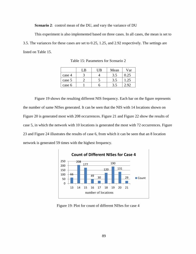
89

Scenario 2: control mean of the DU, and vary the variance of DU

This experiment is also implemented based on three cases. In all cases, the mean is set to

3.5. The variances for these cases are set to 0.25, 1.25, and 2.92 respectively. The settings are

listed on Table 15.

Table 15: Parameters for Scenario 2

LB UB Mean Var case 4 3 4 3.5 0.25 case 5 2 5 3.5 1.25 case 6 1 6 3.5 2.92

Figure 19 shows the resulting different NIS frequency. Each bar on the figure represents

the number of same NISes generated. It can be seen that the NIS with 14 locations shown on

Figure 20 is generated most with 208 occurrences. Figure 21 and Figure 22 show the results of

case 5, in which the network with 10 locations is generated the most with 72 occurrences. Figure

23 and Figure 24 illustrates the results of case 6, from which it can be seen that an 8 location

network is generated 59 times with the highest frequency.

Figure 19: Plot for count of different NISes for case 4

66

208 177

49 30

120

190

131

29

050

100150200250

13 14 15 16 17 18 19 20 21

number of locations

Count of Different NISes for Case 4

Count

90

Figure 20: The NIS with 14 Locations

Figure 21: Plot for count of different NISes for case 5

Figure 22: The NIS With 10 Locations

15

30

50

72

63 60 55

35

60 56 53

61 64 64

45

54 56

33 32

19

7 11

2 3

0

10

20

30

40

50

60

70

80

7 8 9 10 11 12 13 14 15 16 17 18 19 20 21 22 23 24 25 26 27 28 29 30

number of locations

Count of Different NISes for Case 5

Count

91

Figure 23: Plot for count of different NISes for case 6

Figure 24: The NIS with 8 Locations

The experimental results of the two scenarios are summarized on following Table 16 and

Table 17.

Table 16: Results for Scenario 1

Scenario 1 case 1 case 2 case 3 Mean of DU 2 3 4 Var of DU 0.67 0.67 0.67 SSE of NISes 1536.43 2057.84 2546.18 SSEadj 118.19 97.99 82.13 # of locations of the most frequent location network 5 9 16 # of different networks 11 15 18

33 27

33 34 36

59

35 36 36 36 39 42 34 37 36

23

49 41 40

32 35 42

36 29

23 18 17 15

11 11 4

10 5

1 5

0

10

20

30

40

50

60

70

3 5 7 9 11 13 15 17 19 21 23 25 27 29 31 33 35 37

number of locations

Count of Different NISes for Case 6

Count

92

Table 17: Results for Scenario 2

Scenario 2 case 4 case 5 case 6 Mean of DU 3.5 3.5 3.5 Var of DU 0.25 1.25 2.92 SSE of NISes 1397.32 3079.21 4703.04 SSEadj 66.54 99.33 109.37 # of locations of the most frequent location network 14 10 8 # of different networks 9 24 35

From the SSE perspective, as shown in Table 16, when the variance of DU is controlled,

the SSE increases with the increase of mean of DU; and, when the mean of DU is controlled, as

shown in Table 17, the SSE increases with the increase of variance of DU.

From the adjusted SSE perspective, when the variance of DU is controlled, the SSEadj

decreases with the increase of mean of DU; and, when the mean of DU is controlled, the SSEadj

increases with the increase of variance of DU.

From the number of different networks generated, the number of different networks

generated is increased considerably following the increase of the mean while the variance is kept

unchanged (Table 16); and when the mean is kept unchanged, the number of different networks

generated is also increased considerably following the increase of the variance (Table 17).

From the number of locations of the most frequently generated perspective, in scenario 1,

the number of locations of the most frequently generated increases following increase of mean;

and, in scenario 2 it decreases following increase of variance. This helps to diversify generation

of NIS, and since NITs are generated based on NISes, therefore it decides the diversity of NITs

indirectly.

93

4.2.4.3 Diversity of NIT

The diversity of NIT is affected by two parameters: number of retailers at lowest echelon

(NR) and probability of existence of an item at a retail store (PE). Two sets of experiments are

implemented to investigate the impact of these two parameters on the diversity of NITs

generated. The experiments can be summarized as: (1) control the NR and investigate how PE

affects the adjusted SSE; and (2) investigate how NR affects the adjusted SSE.

Experiment 1

This experiment is carried out based on the NIS, which has four retailers. The PEs used

to generate the NIT are 0.1, 0.3, 0.5, 0.7, and 0.9. Using these PEs, 1000 NITs are generated and

the resulting adjusted SSEs are plotted in Figure 25.

Figure 25: Adjusted SSE of 4 Retailers

For each PE, the distributions of the generated NITs are plotted as shown in Figure 26 to

Figure 30. In the figures from Figure 26 to Figure 30, 1 to 4 on the horizontal axis are the NITs

with 1 retailer; 5-10 are the NITs with 2 retailers; 11-14 are the NITs with 3 retailers; and 15 is

the NITs with 4 retailers.

138.28 159.31 165.98

135.25

60.28

0.00

50.00

100.00

150.00

200.00

0 0.2 0.4 0.6 0.8 1

Adjusted SSE: 4 Retailers

adjSSE

94

Figure 26: Plot for count of different NITs when PE=0.1

Figure 27: Plot for count of different NITs when PE=0.3

Figure 28: Plot for count of different NITs when PE=0.5

0

50

100

150

200

250

1 2 3 4 5 6 7 8 9 10 11 12 13 14 15

Count: PE=0.1

Count

0

50

100

150

200

1 2 3 4 5 6 7 8 9 10 11 12 13 14 15

Count: PE=0.3

Count

0

20

40

60

80

100

1 2 3 4 5 6 7 8 9 10 11 12 13 14 15

Count: PE=0.5

Count

95

Figure 29: Plot for count of different NITs when PE=0.7

Figure 30: Plot for count of different NITs when PE=0.9

Based on the results of experiment 1, the following conclusions can be made:

(1) The adjusted SSEs of NITs increase when PE has range 0.1 to 0.5 and decrease when

it has range 0.5 to 1.

(2) When the values of PE increase, the generated NITs tend to have larger number of

locations.

Experiment 2

In order to investigate how NR affects the adjusted SSE of the generated NITs, the values

of NR are set to 3, 4 and 5. Since PE also affects the SSE of the generated NIT, five values of PE,

i.e., 0.1, 0.3, 0.5, 0.7, and 0.9, are used to generate NITs for each value of NR. For experiment 2,

1000 NITs are generated to calculate SSE, and the experiment results are summarized in Table

050

100150200250300

1 2 3 4 5 6 7 8 9 10 11 12 13 14 15

Count: PE=0.7

Count

0

200

400

600

800

1 2 3 4 5 6 7 8 9 10 11 12 13 14

Count: PE=0.9

Count

96

18. For 3 retailer and 5 retailer cases, the changing patterns of SSE according to different PEs are

illustrated in Figure 31 and Figure 32.

Table 18: Experiment Results for Experiment 2

PE Adjusted SSE for 3 NR Adjusted SSE for 4 NR Adjusted SSE for 5 NR 0.1 140.06 138.28 131.95 0.3 148.65 159.31 164.35 0.5 147.50 165.98 178.39 0.7 121.45 135.25 152.35 0.9 49.63 60.28 62.85

Figure 31: Adjusted SSE of 3 Retailers

Figure 32: Adjusted SSE of 5 Retailers

140.06 148.65 147.50

121.45

49.63

0.0020.0040.0060.0080.00

100.00120.00140.00160.00

0 0.2 0.4 0.6 0.8 1

Adjusted SSE: 3 Retailers

adjSSE

131.95

164.35 178.39

152.35

62.85

0.00

50.00

100.00

150.00

200.00

0 0.2 0.4 0.6 0.8 1

Adjusted SSE: 5 Retailers

adjSSE

97

Based on the results of experiment 2, the following can be concluded:

(1) Adjusted SSEs of NITs increase when PE ranges from 0.1 to 0.5 and decrease when it

ranges from 0.5 to 1 for different values of NR.

(2) It can be seen from Table 18 that when PE equals 0.1, the adjusted SSE decreases

with the increasing of NR. When the value of PE is larger than 0.1, the adjusted SSE increases

with the increasing of NR.

These conclusion help to set PE values when generating NITs, for example, to get higher

SSE, which is the diversity measurement of diversity of NITs, for NITs generated, one can set

PE value closer to 0.5.

4.2.4.4 Data Generation and Grouping of the data

As part of the evaluation process of the generated data, this section first illustrates the

generated data using normalized Euclidean Distance between items and the Mean Item. The

Mean Item is obtained by averaging attribute values of all items generated. And then, the

generated items are tentatively grouped using K-Means clustering to see whether the generated

data is “good” for grouping.

In this instance of data, the structure of the NIS is a two echelon inventory system with

one location on echelon 1 and two locations on echelon 2. The figure of the NIS can be found in

Figure 7(B). Using the data generation process discussed in section 4.2.2, and the mechanism

discussed in section 4.2.3.2, which generates the values of the attributes keeping the relations, 20

items were generated. The attributes listed in section 3.3.3, i.e. the attribute list for non-structural

attributes (attribute list 1) and the attribute list for both structural and non-structural attributes

(attribute list 2) are discussed respectively. For each item, normalized Euclidean distances

98

between its attributes and the Mean Item attributes based on both attribute lists 1 and attribute

lists 2 are calculated and stored in Table 19.

Table 19: The Euclidean Distance between Items and the Mean Item

Item# Distance of Non-Structural Attributes

Distance of Non-Structural and Structural Attributes

1 3.58 4.29 2 0.79 0.89 3 2.01 2.12 4 2.87 3.57 5 0.95 1.05 6 2.75 3.35 7 3.03 3.63 8 1.69 1.79 9 4.2 4.9

10 2.62 3.23 11 1.84 1.94 12 2.53 2.63 13 2.9 3.6 14 2.08 2.19 15 2.15 2.25 16 1.42 1.52 17 3.57 4.17 18 1.89 2 19 2.9 3.5 20 1.28 1.38

In order to visualize the distances between items, the normalized Euclidean distances

between items and the Mean Item are drawn in Figure 33 for both attribute list 1 and attribute list

2. It can be seen from Figure 33 that, there are three items, which are item 4, 13 and 19, having

different relative distances (or the relative sequence based on the distance) to the Mean Item; this

means that when applying attributes in list 1 and list 2 separately, the items show different

grouping tendency when the grouping is based on the Euclidean Distance.

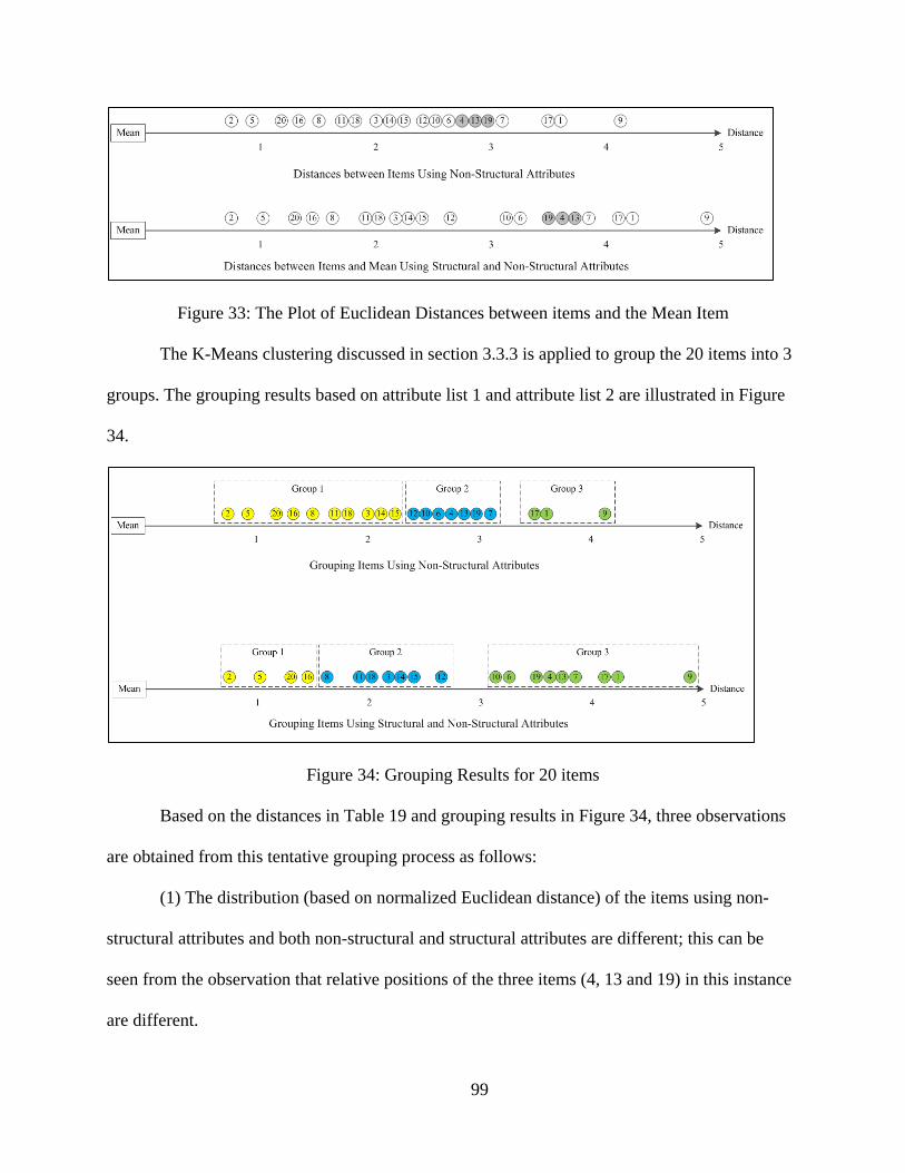
99

Figure 33: The Plot of Euclidean Distances between items and the Mean Item

The K-Means clustering discussed in section 3.3.3 is applied to group the 20 items into 3

groups. The grouping results based on attribute list 1 and attribute list 2 are illustrated in Figure

34.

Figure 34: Grouping Results for 20 items

Based on the distances in Table 19 and grouping results in Figure 34, three observations

are obtained from this tentative grouping process as follows:

(1) The distribution (based on normalized Euclidean distance) of the items using non-

structural attributes and both non-structural and structural attributes are different; this can be

seen from the observation that relative positions of the three items (4, 13 and 19) in this instance

are different.

100

(2) The generated items show some data patterns that can be grouped, which means that

items “visually near” based on normalized Euclidean distance tend to be grouped together.

(3) For the same dataset, the grouping results could be different when using different

grouping attributes.

The generated data in this research will be systematically evaluated further in the

following chapters based on more specific and larger data instances.

101

5 Experimental Design

Based on the guidelines for designing an experiment suggested by Montgomery (2001),

this chapter identifies the research problems; selects the factors, levels to answer the research

questions; the corresponding response variables for the questions; and, the experimental designs

accordingly. This chapter first investigates the research factors and their levels, and then

discusses the experimental design for this research.

5.1 Research Factors Analysis

As illustrated in Exhibit 1, the research factors considered are categorized into 5 main

factor categories. The inventory control policy studied in this dissertation is continuous reorder

point reorder quantity policy; this factor is fixed to one level. Also, the cost model is fixed to the

cost model discussed in 3.2. Except for these two factors, the impacts of other three main factor

categories are studied in this research. This section investigates these main research factor

categories and the levels of the factors.

5.1.1 The Factor Category 𝑁

The factor Category 𝑁 (characteristics of the inventory system) can be classified into

three sub-categories. The 1st category is non-structural attributes. There are 9 factors belonging

to this category, and they can be found in Table 7. The 2nd category is structural attributes;

number of locations, number of echelons and NIT is considered for this category. The 3rd

category is the number of items. The 1st and 2nd categories are the characteristics of one single

item, and the 3rd category describes the scale of the items involved.

102

5.1.2 The factor category 𝑨𝑨 and 𝒌

The factor category 𝐴𝑞 is the grouping methods. Three grouping techniques were

discussed in section 3.3. The study of this factor is a focus of this dissertation. This sub-section

discusses the research questions that are specific for ABC classification and K-Means clustering.

5.1.2.1 Research Questions regarding ABC Classification

The research questions are considered from two perspectives: 1) classification criterion

and 2) the number of groups.

1) The classification criterion

In order to evaluate the effectiveness of the clustering criterion NIC, the traditional ABC

classification criterion, i.e., annual dollar usage is also implemented. The formula used to

calculate the network annual dollar usage (𝑁𝐴𝐷𝑈) is as following:

𝑁𝐴𝐷𝑈 = ��𝜆𝑖𝑗 × 𝐼𝑖

𝑟

𝑗=1

𝑛

𝑖=1

Where

𝑛 ≡ number of item types

𝑟 ≡ number of retail stores

𝐼𝑖 ≡ unit cost of item i

𝜆𝑖𝑗 ≡ annual demand of item i at location j

2) The number of groups

As discussed in Teunter et al. (2010), typical A, B, and C classes contain around 20%,

30%, and 50% of all SKUs respectively. Teunter et al. (2010) proposes an extension of 3 classes

to 6 classes ABC classification with 4% for A class, 7% for B class, 10% for C class, 16 % for D

class, 25% for E class, and 38% for F class. In this research, the typical three classes ABC

103

classification, and a seven classes ABC classification extended from Teunter et al. (2010)’s 6

classes ABC classification are implemented. The details about the extension from 6 classes to 7

classes are introduced in section 6.2.

In sum, there are two specific research questions related to ABC Classification:

A1: Whether the classification criterion NIC is better than NADU?

A2: Whether 7-group is better than 3-group for ABC classification?

5.1.2.2 Research Questions regarding K-Means Clustering

Six K-Means Clustering related research questions are discussed in this section.

K1: Which non-structural attributes are significant?

The selection of clustering attributes is critical for K-Means clustering. From the

efficiency perspective, the more clustering attributes, the more clustering time will be taken. Too

many clustering attributes may make clustering time infeasible. From the effectiveness

perspective, adding some not significant clustering attributes may reduce the system performance.

Thus, this research question is to identify the significant non-structural attributes.

K2: Whether the item types having the same NIT structure tend to be clustered into the

same group?

After grouping the items using the K-Means clustering, a study of main NIT is performed

to identify the dominating structure in each group. An example of main NIT analysis is

illustrated in Table 33. If in each group, a majority of items have the same NIT structure, then it

can be concluded as a trend that to group items with same NIT together exists.

K3: Whether the structural attributes affect the clustering results?

The structural attribute considered in this research is NIT. The binary expression for NIT

(illustrated in Table 4) is used as the structural attributes values for K-Means. In other words, the

104

structural attributes is a set of binary variables, each of which represent the existence of a retail

store. Experiments are designed to test the changes of effectiveness and efficiency when

structural attributes are involved.

K4: Which factors affect the K-Means clustering time?

The clustering time (in seconds) is crucial for large scale grouping. Maimon and Rokach

(2005) summarize three factors affecting the K-Means clustering time: the number of instances,

the number of clusters, and the number of iterations used by the algorithm to converge. Besides

these three factors, the number of clustering attributes is also considered for the study of

clustering time.

K5: How does the number of clusters k affect the clustering results?

As mentioned previously, the number of clusters affects clustering performance which

are measured based on %CPC (Percent Grouping Penalty Cost), SSE, and GT (Grouping Time)

in this research. Two levels of k, i.e., 3 and 7 groups are used to investigate the changes of the

selected performance measures.

5.1.2.3 Research Questions for comparing different grouping techniques

The three grouping techniques, ABC, NIT, and K-means need to be compared based on

the same number of groups. Since NIT classification can have 7 groups when the number of

retailer locations is 3, and the number of groups for ABC classification can be legitimately

extended to 7 groups, while K-means clustering has the flexibility of setting the number of

groups K, the number of groups for comparison of the grouping techniques is set to 7 groups.

Basing the comparison of the grouping techniques on 7 groups rather than 3 groups is also

because 7-group case results better performance measures for both ABC and K-means grouping

techniques.

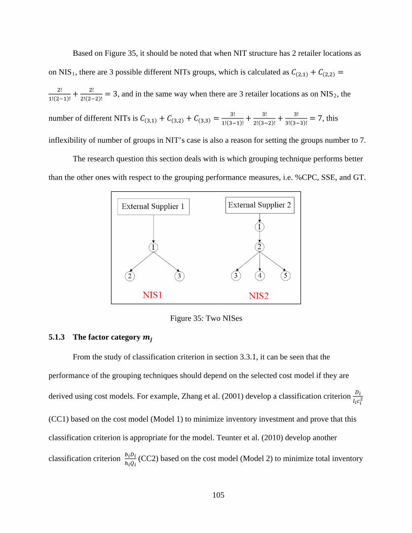
105

Based on Figure 35, it should be noted that when NIT structure has 2 retailer locations as

on NIS1, there are 3 possible different NITs groups, which is calculated as 𝐼(2,1) + 𝐼(2,2) =

2!1!(2−1)!

+ 2!2!(2−2)!

= 3, and in the same way when there are 3 retailer locations as on NIS2, the

number of different NITs is 𝐼(3,1) + 𝐼(3,2) + 𝐼(3,3) = 3!1!(3−1)!

+ 3!2!(3−2)!

+ 3!3!(3−3)!

= 7, this

inflexibility of number of groups in NIT’s case is also a reason for setting the groups number to 7.

The research question this section deals with is which grouping technique performs better

than the other ones with respect to the grouping performance measures, i.e. %CPC, SSE, and GT.

Figure 35: Two NISes

5.1.3 The factor category 𝒎𝒎

From the study of classification criterion in section 3.3.1, it can be seen that the

performance of the grouping techniques should depend on the selected cost model if they are

derived using cost models. For example, Zhang et al. (2001) develop a classification criterion 𝐷𝑖𝑙𝑖𝑐𝑖

2

(CC1) based on the cost model (Model 1) to minimize inventory investment and prove that this

classification criterion is appropriate for the model. Teunter et al. (2010) develop another

classification criterion 𝑏𝑖𝐷𝑖ℎ𝑖𝑄𝑖

(CC2) based on the cost model (Model 2) to minimize total inventory

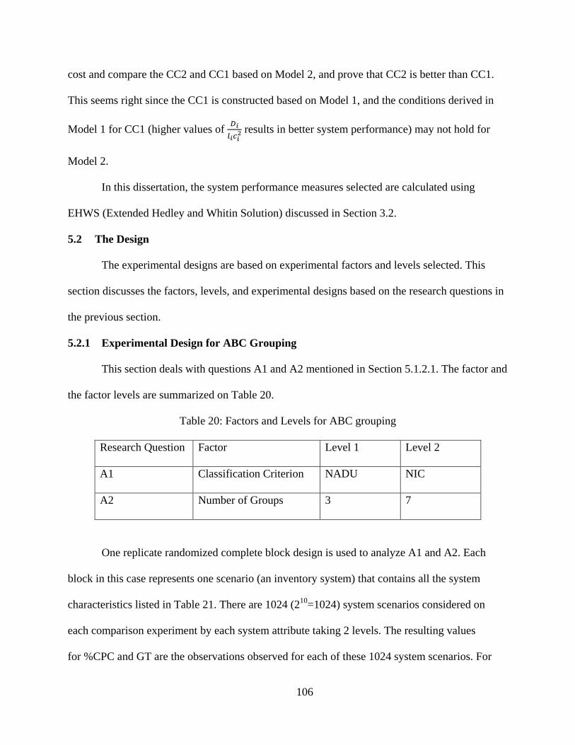
106

cost and compare the CC2 and CC1 based on Model 2, and prove that CC2 is better than CC1.

This seems right since the CC1 is constructed based on Model 1, and the conditions derived in

Model 1 for CC1 (higher values of 𝐷𝑖𝑙𝑖𝑐𝑖

2 results in better system performance) may not hold for

Model 2.

In this dissertation, the system performance measures selected are calculated using

EHWS (Extended Hedley and Whitin Solution) discussed in Section 3.2.

5.2 The Design

The experimental designs are based on experimental factors and levels selected. This

section discusses the factors, levels, and experimental designs based on the research questions in

the previous section.

5.2.1 Experimental Design for ABC Grouping

This section deals with questions A1 and A2 mentioned in Section 5.1.2.1. The factor and

the factor levels are summarized on Table 20.

Table 20: Factors and Levels for ABC grouping

Research Question Factor Level 1 Level 2

A1 Classification Criterion NADU NIC

A2 Number of Groups 3 7

One replicate randomized complete block design is used to analyze A1 and A2. Each

block in this case represents one scenario (an inventory system) that contains all the system

characteristics listed in Table 21. There are 1024 (210=1024) system scenarios considered on

each comparison experiment by each system attribute taking 2 levels. The resulting values

for %CPC and GT are the observations observed for each of these 1024 system scenarios. For

107

CPC and %CPC calculation process refer to Section 3.3.5.2. A complete block is an

experimental setup that tests the two levels of the factors by putting them in one scenario. For

example, for A1 use both NIC and NADU to implement ABC classification; for A2 use both 3

groups and 7 groups to implement ABC classification. In an experiment, randomization is used

to control unknown and uncontrolled nuisance factors (Montgomery (2001)). For example, setup

time is one of the uncontrolled nuisance factors. When running a 1024-scenario experiment, at

the beginning the computer start allocating resources such as RAM for the calculation, therefore

the scenarios implemented during this period run relatively slowly than the scenarios

implemented after the setting up; this results in the variances on GT. To control the effect of the

setting up process to the experimental results, the randomization is implemented by randomizing

the sequence of the levels within each block experiment.

Table 21: The Factor Index for Item Characteristics

Factor Index Attribute Low High A Unit Cost ($) [1,10] [1,20] B Lost-Sale-Cost-to-Unit-Cost Ratio [0.1,0.2] [0.1, 0.5] C Ordering Cost ($) [10,20] [10,50] D Inventory Holding Charge ($/$/year) [1%,10%] [1%,20%] E Demand Rate (yearly) [1,100] [1,200] F Demand Variance-to-Mean Ratio [0.1,0.2] [0.1, 0.5] G Mean lead time at ES (day) [10,20] [10,50] J Lead Time Variance-to-Mean Ratio [0.1,0.2] [0.1, 0.5] K Number of Items 1100 2200 L Number of IHPs 3 5

Since there are 1 factor 2 level in dealing with A1 and A2, Paired t-test is used to analyze the

performance measures %CPC and GT.

5.2.2 Experimental Design for K-Means Clustering

The research question K1 is to identify the most significant non-structural attributes for

the grouping process. As shown in Table 21, 8 (A to J) factors (attributes) are investigated to

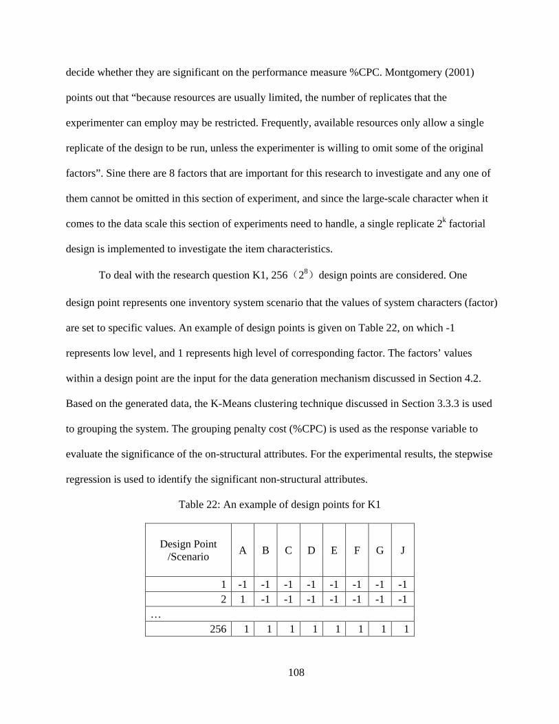
108

decide whether they are significant on the performance measure %CPC. Montgomery (2001)

points out that “because resources are usually limited, the number of replicates that the

experimenter can employ may be restricted. Frequently, available resources only allow a single

replicate of the design to be run, unless the experimenter is willing to omit some of the original

factors”. Sine there are 8 factors that are important for this research to investigate and any one of

them cannot be omitted in this section of experiment, and since the large-scale character when it

comes to the data scale this section of experiments need to handle, a single replicate 2k factorial

design is implemented to investigate the item characteristics.

To deal with the research question K1, 256（28）design points are considered. One

design point represents one inventory system scenario that the values of system characters (factor)

are set to specific values. An example of design points is given on Table 22, on which -1

represents low level, and 1 represents high level of corresponding factor. The factors’ values

within a design point are the input for the data generation mechanism discussed in Section 4.2.

Based on the generated data, the K-Means clustering technique discussed in Section 3.3.3 is used

to grouping the system. The grouping penalty cost (%CPC) is used as the response variable to

evaluate the significance of the on-structural attributes. For the experimental results, the stepwise

regression is used to identify the significant non-structural attributes.

Table 22: An example of design points for K1

Design Point /Scenario A B C D E F G J

1 -1 -1 -1 -1 -1 -1 -1 -1 2 1 -1 -1 -1 -1 -1 -1 -1

…

256 1 1 1 1 1 1 1 1

109

5.2.3 Experimental Design for Comparing the Three Grouping Methods

The goal of the experiment is to compare the three grouping methods. The research factor

is the grouping method, and there are three factor levels, i.e., ABC classification, NIT

classification, and K-Means clustering implemented in this research.

The experiments implement one replicate randomized complete block design. Each block

in this case represents one scenario (inventory system). A complete block is an experimental

setup that tests the three methods by putting them in one scenario. The randomization is

implemented by randomizing the sequence of the experiments corresponding to each of the

grouping methods within each block. To compare the grouping methods based on 7 groups, the

number of IHP is seleceted as 5 (3 echelon 3-retailer case). The 9 attributes with indices from A

to K on Table 21 are considered on each experiment. There are 512 (29=512) system scenarios

(blocks) considered on each comparison experiment. In this three grouping method comparison

experiment, since the grouping method factor has 3 levels, therefore there are three design points

as shown on Table 23. The resulted block design is shown on Table 24. Each scenario (block) is

generated using the data generation mechanism discussed in Section 4.2.

Table 23: Design Points for the Three Grouping Method Comparison

Design Point Grouping Method 1 ABC classification 2 NIT classification 3 K-Means clustering

Table 24: Block Design for the Three Grouping Method Comparison

Grouping Method Block 1 2 … 512

(1)ABC classification y11 y12 … y1_512 (2)NIT classification y21 y22 … y2_512 (3)K-Means clustering y31 y32 … y3_512

110

The response variables for the experiments are %CPC, SSE, and GT. ANOVA is used to

analyze the experimental results. If the null hypotheses are rejected, the Fisher’s LSD method is

used to conduct multiple comparisons.

111

6 Experimental Results and Analysis

The datasets generated for the experiments in this chapter are based on the analysis of the

system characteristics of large scale multi-item, multi-echelon inventory systems in the previous

sections. The non-structural and structural attributes selected for the grouping are listed on Table

21. As discussed in the previous sections these attributes are chosen based on the inventory

system characteristics summarized in Cohen et al. (1986) and the cost model used in this

research. The data generation process is summarized on Section 4.2.2.2. The relationships

between the attributes generated are introduced in Section 4.2.3.2.

Based on the data generation mechanism discussed on chapter 4, values of the system

characteristics for the experiments in this chapter are generated. To introduce the generated

attribute values and their characteristics, a pilot experiment is presented. Using this pilot

experiment the three grouping methods are implemented based on three attributes, i.e. Unit Cost,

Ordering Cost (on a specific location), and Demand Rate (on a specific location) to illustrate the

relationships between clusters and the performance measures, i.e. %CPC and SSE, visually. Also,

in this pilot experiment, the consistency between these performance measures is visually

presented. After clarifying these relationships, the following sections implement more specific

experiments regarding the grouping methods of interest based on the same data generation

mechanism.

Following the pilot experiment, rest of this chapter analyzes the experimental results of

ABC classification and K-Means clustering, and then the comparison of the three individual

grouping techniques is conducted.

112

6.1 Pilot Experiment

This section presents some pilot experiments to help better understanding of the

following experiments carried out in rest of this chapter using visual tools, such as plots, charts,

etc.

6.1.1 Data for Pilot Experiment

The NIS selected (the NIS2 as shown in Figure 35) for this part of the experiment is a

three-echelon structure, which has one location on echelon 1, one location on echelon 2, and

three locations on echelon 3. Since the goal is to show visually the experimental results in this

section, only one scenario is considered. The high level ranges of the non-structural attributes as

shown on Table 21 are selected as the attribute value ranges in this part of experiment, except the

value of number of items, which is set as 10000.

For overall generated data, we need more spread out data with some data points

compacted in certain areas so that we can check whether the grouping methods are grouping the

compacted data together. To present better the grouping mechanism visually, the following steps

are taken to generate data that shows clear pattern:

1) Use data generation mechanism mentioned in Chapter 4 to generate 10,000 items. The

generated data is plotted in Figure 36 to visualize the data points. In Section 6.3.1, the

significance of non-structural attributes is studied using stepwise regression analysis. The results

show that ordering cost, demand and unit cost are the most significant non-structural attributes

which affect the grouping penalty cost; thus, these three attributes are selected to plot the items.

In addition, the items located at location 3 are selected to plot the items. The values of the

selected attributes are normalized to plot the data points as shown in Figure 36.

113

Figure 36: 10,000 Items

2) It should be noted that the data points on Unit Cost axis represent the item types that

are not stored at location 3, and this can be seen based on the NIT structures on Figure 37. On

Figure 37, it can be seen that the item types stored at location 3 have NITs as shown on part (a),

and the item types not stored at location 3 have NITs as shown on part (b). It can also be seen

from the plot that the NIT structure, which represents an item type’s storage structure in an

inventory network, affects the data pattern as shown on Figure 36.

114

Figure 37: NIT structures

As mentioned in Lenard and Roy (1995), the storage structure is the attribute that prevent

items grouping together. NIT represents the storage structure of a specific item type in an

inventory network, and it represents the supplier and customer relationships between the

locations for the item type. Therefore, it can be seen that the data points on the Unit Cost axis

tend to be clustered separate to the other data points that not falling on to the Unit Cost axis.

The goal of the data generation in this pilot experiment section is to obtain data points

with clear cluster patterns visually (in 3D plot). To obtain this kind of data points, the entire

space shown on Figure 36 is divided into 27 cubic spaces based on Table 25, on which LB and

UB represent Lower Bound and Upper Bound respectively.

115

Table 25: 27 Modules

Module Unit Cost Demand Ordering Cost LB UB LB UB LB UB

1 0.15 0.4 0.15 0.4 0.15 0.4 2 0.15 0.4 0.15 0.4 0.45 0.7 3 0.15 0.4 0.15 0.4 0.75 1 4 0.15 0.4 0.45 0.7 0.15 0.4 5 0.15 0.4 0.45 0.7 0.45 0.7 6 0.15 0.4 0.45 0.7 0.75 1 7 0.15 0.4 0.75 1 0.15 0.4 8 0.15 0.4 0.75 1 0.45 0.7 9 0.15 0.4 0.75 1 0.75 1

10 0.45 0.7 0.15 0.4 0.15 0.4 11 0.45 0.7 0.15 0.4 0.45 0.7 12 0.45 0.7 0.15 0.4 0.75 1 13 0.45 0.7 0.45 0.7 0.15 0.4 14 0.45 0.7 0.45 0.7 0.45 0.7 15 0.45 0.7 0.45 0.7 0.75 1 16 0.45 0.7 0.75 1 0.15 0.4 17 0.45 0.7 0.75 1 0.45 0.7 18 0.45 0.7 0.75 1 0.75 1 19 0.75 1 0.15 0.4 0.15 0.4 20 0.75 1 0.15 0.4 0.45 0.7 21 0.75 1 0.15 0.4 0.75 1 22 0.75 1 0.45 0.7 0.15 0.4 23 0.75 1 0.45 0.7 0.45 0.7 24 0.75 1 0.45 0.7 0.75 1 25 0.75 1 0.75 1 0.15 0.4 26 0.75 1 0.75 1 0.45 0.7 27 0.75 1 0.75 1 0.75 1

To obtain 7 groups of data showing clustering patterns that this section of experiments

require, 6 spaces with the largest number of data points and the Unit Cost axis data points are

selected (this is to keep the location related attributes in the clustering patterns). To obtain

clusters that having enough between cluster distances, the spaces of data points that close to

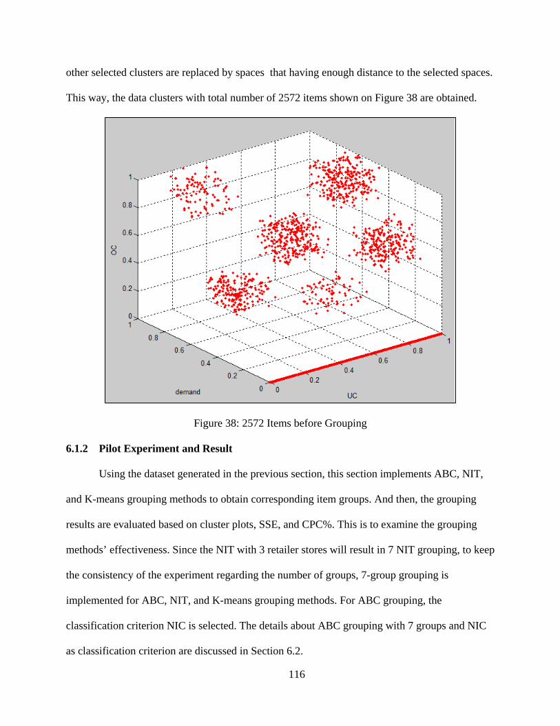
116

other selected clusters are replaced by spaces that having enough distance to the selected spaces.

This way, the data clusters with total number of 2572 items shown on Figure 38 are obtained.

Figure 38: 2572 Items before Grouping

6.1.2 Pilot Experiment and Result

Using the dataset generated in the previous section, this section implements ABC, NIT,

and K-means grouping methods to obtain corresponding item groups. And then, the grouping

results are evaluated based on cluster plots, SSE, and CPC%. This is to examine the grouping

methods’ effectiveness. Since the NIT with 3 retailer stores will result in 7 NIT grouping, to keep

the consistency of the experiment regarding the number of groups, 7-group grouping is

implemented for ABC, NIT, and K-means grouping methods. For ABC grouping, the

classification criterion NIC is selected. The details about ABC grouping with 7 groups and NIC

as classification criterion are discussed in Section 6.2.

117

The grouping results of K-means, NIT, and ABC are plotted as on Figure 39, Figure 40,

and Figure 41. The resulted SSE and CPC% values are summarized on Table 26. In Figure 39 to

Figure 41, each color represents items which are grouped in the same group. It can be seen from

Figure 39 that K-means results the completely separated clusters with unique color for each

cluster. For the convenience in the rest of this research, the clusters grouped by K-means

clustering are referred as K-Means cluster. Figure 40 and Figure 41 show the NIT and ABC

grouping results with mixed colors compared to corresponding K-Means clusters. This indicates

that items which are close to each other based on the distance of ordering cost, demand and unit

cost are grouped together when K-means clustering is used, but are separated to different groups

when NIT and ABC classification are applied. It should be noted that, on Figure 40, the clusters

not on Unit Cost axis are mixed with 4 colors, while Unit Cost axis clusters are mixed with 3

colors. This is due to the structures shown on Figure 37, i.e., the items on Unit Cost Axis belongs

to one of the three structures in part (b) of the figure, and remaining ones belong to one of the

structures in part (a) of the figure. And, on Figure 41, all the clusters are mixed with 7 colors.

From the degree of mixture of the colors, it can be seen that NIT clusters are better grouped than

ABC’s, for items which are close to each other based on the distance of ordering cost, demand

and unit cost are separated to more different groups in ABC than in NIT classification. This is

consistent with the corresponding SSE and CPC% results in Table 26. On Table 26, both SSE

and CPC% values of K-means clustering are lower than NIT and ABC’s; while NIT’s SSE and

CPC% values are lower than ABC’s.

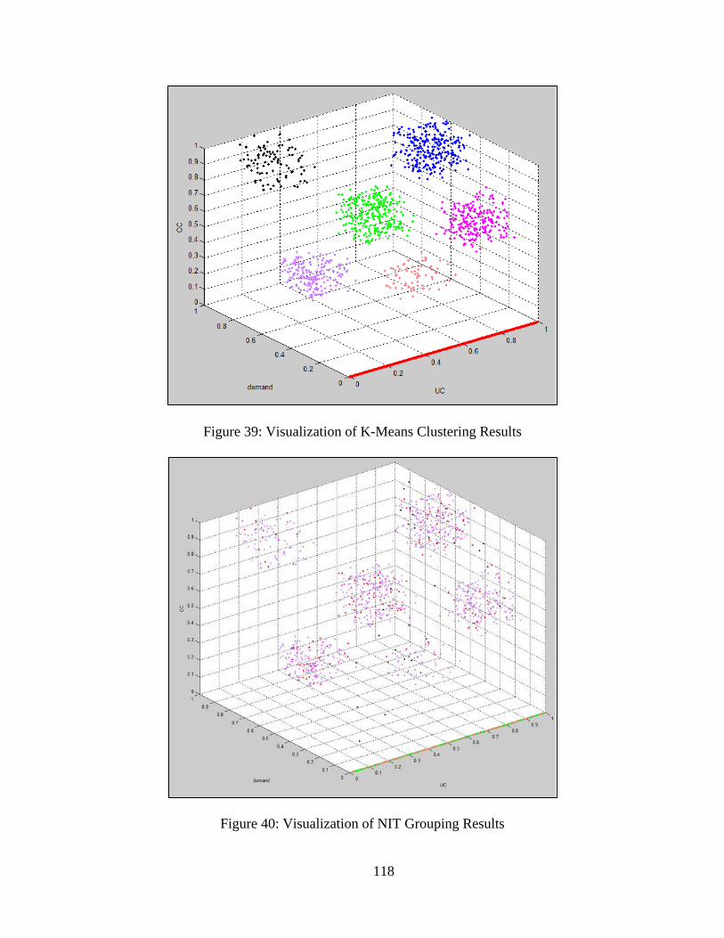
118

Figure 39: Visualization of K-Means Clustering Results

Figure 40: Visualization of NIT Grouping Results

119

Figure 41: Visualization of ABC Grouping Results

Table 26: Grouping Result of Three Method

%CPC SSE K-Means 9.2 10.78

NIT 10.4 3350.27 ABC 12.3 4342.32

It can be seen from the results that the visual results (plots), the SSE and CPC% are

consistent. This consistency can be found between SSE and CPC% values; this is because CPC%

as SSE also reflects the distance (difference) between items that are grouped.

The following two tables, Table 27 and Table 28, show the percentage of items that are in

common between K-means groups and ABC groups and between K-Means groups and NIT

groups respectively. Since K-means performs the best in grouping, it is taken as benchmark in

these comparisons. In the tables, the decimal numbers represent the percentage of the items that

common in the grouping results for both of the grouping methods compared. In Table 27, not

120

including the last row, each column on the table is the comparison between each ABC resulted

group against all the K-means resulted groups. The resulting maximum percentage from the

comparison is put on the last row. This percentage is taken as the maximum similarity percentage

between one ABC group and all the K-means groups. It can be seen from Table 27 that

maximum percentage similarity ranges from 0.13 to 0.53 for the comparison of K-means and

ABC methods. Similarly, it can be seen from Table 28 that the maximum percentage similarity

ranges from 0.06 to 0.72 for the comparison of K-means and NIT methods. When comparing

ABC and NIT groups to K-means groups, since the average maximum similarity percentage in

ABC case is 28.71% and it’s 30.29% in NIT case, it can be concluded that relative to ABC

method, NIT results more similar groups to K-means method.

Table 27: Common items within groups between K-means and ABC

K-means Group/ABC Group 1 2 3 4 5 6 7 1 0.53 0.01 0.02 0.04 0.06 0.11 0.24 2 0.02 0.06 0.09 0.18 0.24 0.27 0.15 3 0.01 0.13 0.21 0.18 0.16 0.21 0.1 4 0.1 0.01 0.06 0.07 0.17 0.33 0.26 5 0.38 0 0 0.02 0.07 0.17 0.36 6 0.11 0.08 0.08 0.08 0.22 0.21 0.23 7 0.08 0 0.02 0.08 0.16 0.26 0.39

Max% 0.53 0.13 0.21 0.18 0.24 0.33 0.39

Table 28: Common items within groups between K-means and NIT

K-means Group/NIT Group 1 2 3 4 5 6 7 1 0 0.74 0.13 0.13 0 0 0 2 0.15 0 0 0 0.72 0.12 0.02 3 0.14 0 0 0 0.73 0.11 0.02 4 0.09 0 0 0 0.77 0.09 0.06 5 0.15 0 0 0 0.7 0.12 0.02 6 0.11 0 0 0 0.76 0.1 0.04 7 0.1 0 0 0 0.79 0.09 0.01

Max% 0.15 0.74 0.13 0.13 0.79 0.12 0.06

121

In this section, the three grouping methods are compared using the three attributes selected,

and the results are visually presented using figures. The results show that K-means has lowest

CPC% and SSE. More comprehensive investigation and comparison of these methods are carried

out in the following sections.

6.2 Analysis of ABC Classification results

This part of experiment is to answer questions A1 and A2 mentioned in Section 5.1.2.1.

12 factors are used in this ABC classification experiment, including all the characteristics of item

types (10 factors listed in Table 21) plus number of groups (NG) and classification criterion. The

same scenarios (210=1024) are used for both levels of A1 and A2, and the sequence of the levels

are randomly decided; therefore, the randomized complete block designs are implemented for

dealing with questions A1 and A2 respectively.

A1：whether the classification criterion NIC is better than NADU?

The two classification criteria are compared based on two response variables, the

percentage of clustering penalty cost (%CPC) and the grouping time (GT). The %CPC indicates

the effectiveness of the grouping technique, and GT represents the efficiency of the grouping

technique.

The comparisons of the across scenario means of %CPC and GT for NADU and NIC are

shown in Figure 42. The Appendix 5 illustrates the organization of the experimental results and

the calculation of the across scenario means.

122

Figure 42: Comparisons between NADU and NIC

Figure 42 shows that NIC has lower %CPC and shorter GT. Paired t-test is further

implemented to investigate whether there are significant differences between NIC and NADU for

the two response variables. Paired t-test is the most appropriate analysis in this case because (1)

the NIC and NADU are calculated based on the same scenarios (subjects), and their calculations

involve the same inputs such as unit cost and annual demand rate, which satisfy the “related

paired observations” assumption of t-test; and (2) a paired t-test does not require both samples to

have equal variance. The test is based on the mean value of % CPC (percent-clustering penalty

cost) and the mean value of the ABC classification time (GT). Minitab is used for the following

tests.

The NIC and NADU test based on % CPC uses the following hypothesis:

H0: µ1 - µ2 = 0 (% CPC does not change using NIC and NADU)

H1: µ1 - µ2 < 0 (NIC results smaller % CPC than NADU)

(µ1: mean of %CPC for NIC; µ2: mean of %CPC for NADU; α=0.05)

0.0 4.0 8.0 12.0 16.0

Grouping Time(0.01 Second)

%CPC

7.3810

14.22

7.3157

13.88

NICNADU

123

The test results of NIC and NADU testing based on % CPC are shown in Exhibit 24. The

resulted P-Value (0.000) indicates that the mean difference within pairs is statistically significant,

therefore it can be concluded that NIC performs better as an ABC classification criterion than

NADU for the case of interest. This is consistent with the trend shown in Figure 42. It can be

seen that NIC results 0.34% less CPC in average.

Paired T-Test and CI: %CPC_NIC, %CPC_NADU Paired T for %CPC_NIC - %CPC_NADU

N Mean StDev SE Mean

%CPC_NIC 2048 13.8830 1.3361 0.0295

%CPC_NADU 2048 14.2228 1.3390 0.0296

Difference 2048 -0.33979 0.18106 0.00400

95% upper bound for mean difference: -0.33321

T-Test of mean difference = 0 (vs < 0): T-Value = -84.93 P-Value = 0.000

Exhibit 24: Paired T-Test for Penalty Cost (A1)

The NIC and NADU test based on GT uses the following hypothesis:

H0: µ1 - µ2 = 0 (GT does not change using NIC and NADU)

H1: µ1 - µ2 < 0 (NIC results smaller GT than NADU)

(µ1: mean of GT for NIC; µ2: mean of GT for NADU; α=0.05)

Exhibit 25 shows the test results of NIC and NADU testing based on GT. The resulted P-

Value (0.000) indicates that the mean difference within pairs is statistically significant, therefore

it can be concluded that NIC based ABC classification uses considerably less time than NADU.

Paired T-Test and CI: GT_NIC, GT_NADU Paired T for GT_NIC - GT_NADU

N Mean StDev SE Mean

GT_NIC 2049 0.073157 0.039922 0.000882

GT_NADU 2049 0.073810 0.040363 0.000892

Difference 2049 -0.000653 0.005250 0.000116

95% upper bound for mean difference: -0.000462

124

T-Test of mean difference = 0 (vs < 0): T-Value = -5.63 P-Value = 0.000

Exhibit 25: Paired T-Test for Grouping Time (A1)

A2：whether 7 groups are better than 3 groups for ABC classification?

In answering this question, 7 groups are considered due to: 1) to investigate how the

number of groups affects the grouping results for ABC grouping, a group number more than 3

should be selected; 2) the comparison between ABC, NIT and K-Means grouping methods

should be carried out based on same number of groups, and the selected NIT structure allows 7

group classification for the NIT method; 3) Teunter et al. (2010)’s suggestion on the percentage

of number of items for each group for a 6-group ABC classification can be extended

conveniently to the 7-group case.

Teunter et al. (2010) suggests 4%, 7%, 10%, 16%, 25% and 38% for a 6-group ABC

classification case. The ratios between the adjacent two groups in this case can be summarized as

on Table 29; it can be seen that the average of this ratio is 1.57. By lowering this ratio to 1.5, this

research extends the 6-group case to 7-group case as on Table 30.

Table 29: ABC Setup in Teunter et al. (2010)

A B C D E F % 4 7 10 16 25 38 Ratio 1.75 1.43 1.6 1.56 1.52

Table 30: ABC Setup for 7 Groups

A B C D E F G 3 5 7 11 16 23 35

The comparisons of the across scenario means of %CPC and GT for 3 and 7-group cases

are shown in Figure 43.

125

Figure 43: Comparisons between 3 and 7 groups for ABC

Figure 43 shows that 7-group has lower %CPC and slightly longer GT. Paired t-test is

further implemented to investigate whether there are significant differences between 3 and 7-

group cases for the two response variables.

Paired t-test is used for the analysis in this case for the same reasons as mentioned

previously (in A1).

The 3-group and 7-group test based on % CPC uses the following hypothesis:

H0: µ1 - µ2 = 0 (% CPC does not change in 3-group and 7-group cases)

H1: µ1 - µ2 < 0 (7-group case have smaller % CPC than 3-group case)

(µ1: mean of %CPC for 7-group case; µ2: mean of %CPC for 3-group case; α=0.05)

The test results of 3-group and 7-group testing based on % CPC are shown in Exhibit 26.

The resulted P-Value (0.000) indicates that the mean difference within pairs is statistically

significant, therefore it can be concluded that 7-group is better than 3-group grouping for ABC

classification, and the average of %CPC of 7 group is 4.48% lower than that of 3 group case.

This is consistent with the trend shown in Figure 43. This is consistent with the commonly held

view that the more groups the items are divided into the less the resulting penalty cost will be.

0.0 5.0 10.0 15.0

Grouping Time(0.01 Second)

%CPC

7.3456

14.10

7.3587

9.62

73

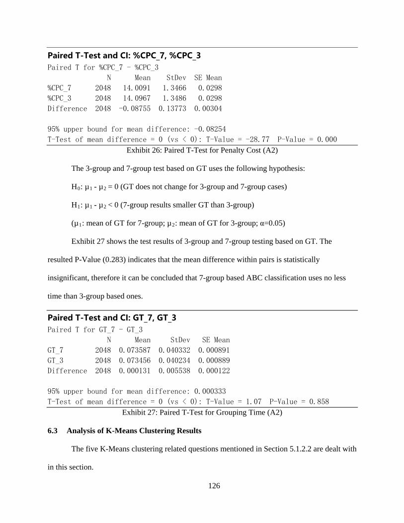
126

Paired T-Test and CI: %CPC_7, %CPC_3 Paired T for %CPC_7 - %CPC_3

N Mean StDev SE Mean

%CPC_7 2048 14.0091 1.3466 0.0298

%CPC_3 2048 14.0967 1.3486 0.0298

Difference 2048 -0.08755 0.13773 0.00304

95% upper bound for mean difference: -0.08254

T-Test of mean difference = 0 (vs < 0): T-Value = -28.77 P-Value = 0.000

Exhibit 26: Paired T-Test for Penalty Cost (A2)

The 3-group and 7-group test based on GT uses the following hypothesis:

H0: µ1 - µ2 = 0 (GT does not change for 3-group and 7-group cases)

H1: µ1 - µ2 < 0 (7-group results smaller GT than 3-group)

(µ1: mean of GT for 7-group; µ2: mean of GT for 3-group; α=0.05)

Exhibit 27 shows the test results of 3-group and 7-group testing based on GT. The

resulted P-Value (0.283) indicates that the mean difference within pairs is statistically

insignificant, therefore it can be concluded that 7-group based ABC classification uses no less

time than 3-group based ones.

Paired T-Test and CI: GT_7, GT_3 Paired T for GT_7 - GT_3

N Mean StDev SE Mean

GT_7 2048 0.073587 0.040332 0.000891

GT_3 2048 0.073456 0.040234 0.000889

Difference 2048 0.000131 0.005538 0.000122

95% upper bound for mean difference: 0.000333

T-Test of mean difference = 0 (vs < 0): T-Value = 1.07 P-Value = 0.858

Exhibit 27: Paired T-Test for Grouping Time (A2)

6.3 Analysis of K-Means Clustering Results

The five K-Means clustering related questions mentioned in Section 5.1.2.2 are dealt with

in this section.

127

6.3.1 The Significant Non-Structural Attributes

This section deals with Question K1 (which non-structural attributes are significant?) in

Section 5.1.2.2. As illustrated in Table 21, the non-structural attributes are indexed with A to J.

The stepwise regression, the most widely used variable selection technique, is applied to find

significant variables. A detailed introduction of stepwise regression can be found in

(Montgomery and Runger 2003). Based on the response variable percentage of clustering penalty

cost (%CPC), Exhibit 28 illustrates the Minitab stepwise regression output for K-Means

clustering with 7 groups for the scenario of 2200 items and 5 IHPs.

Results for: k7-2200items-Ihp5

Regression Analysis: %CPC versus A, B, C, D, E, F, G, J

Stepwise Selection of Terms

Candidate terms: A, B, C, D, E, F, G, J

------Step 1----- ------Step 2------ ------Step 3------

Coef P Coef P Coef P

Constant 4.994 5.825 6.396

C 0.11651 0.000 0.11651 0.000 0.11651 0.000

E -0.01102 0.000 -0.01102 0.000

A -0.03172 0.000

B

D

J

G

S 0.657049 0.597227 0.548275

R-sq 64.06% 70.43% 75.17%

R-sq(adj) 63.92% 70.19% 74.88%

R-sq(pred) 63.49% 69.72% 74.38%

Mallows’ Cp 298.25 202.83 132.13

------Step 4------ ------Step 5------ ------Step 6------

Coef P Coef P Coef P

Constant 7.080 6.451 6.722

C 0.11651 0.000 0.11651 0.000 0.11651 0.000

128

E -0.01102 0.000 -0.01102 0.000 -0.01102 0.000

A -0.03172 0.000 -0.03172 0.000 -0.03172 0.000

B -3.036 0.000 -3.036 0.000 -3.036 0.000

D 7.86 0.000 7.86 0.000

J -1.203 0.002

G

S 0.498906 0.458661 0.450382

R-sq 79.52% 82.76% 83.45%

R-sq(adj) 79.20% 82.42% 83.05%

R-sq(pred) 78.70% 81.93% 82.50%

Mallows’ Cp 67.50 19.91 11.45

------Step 7------

Coef P

Constant 6.891

C 0.11651 0.000

E -0.01102 0.000

A -0.03172 0.000

B -3.036 0.000

D 7.86 0.000

J -1.203 0.001

G -0.00755 0.044

S 0.447605

R-sq 83.72%

R-sq(adj) 83.26%

R-sq(pred) 82.65%

Mallows’ Cp 9.33

α to enter = 0.05, α to remove = 0.05 Exhibit 28: Minitab Stepwise Regression Output

At the level of significance (Alpha) of 0.05, 7 of the 8 factors have significant effect on

the %CPC. Figure 44 is the main effects plot for %CPC. The magnitude of the vertical

displacement indicates the strength of the main effect of the corresponding factor. As shown in

Figure 44, factor with index “C” (Ordering Cost) has significantly stronger effect than any other

factors; therefore, it is the most significant factor. The main effects plot also shows the direction

129

of the main effects. In addition, from the analysis of the stepwise regression results (in Exhibit

28), it can be seen that the main effect plots of factor “F” (Demand Variance-to-Mean Ratio) is

very flat; this means that only factor “F” is not significant when Alpha equals to 0.05. The

residual plot for the analysis of main effects for %CPC is shown in Figure 45. The residual plot

supports the normality assumption of the residuals.

Figure 44: Main Effects Plot for %CPC

Figure 45: Residual Plot for Significant Factor Analysis

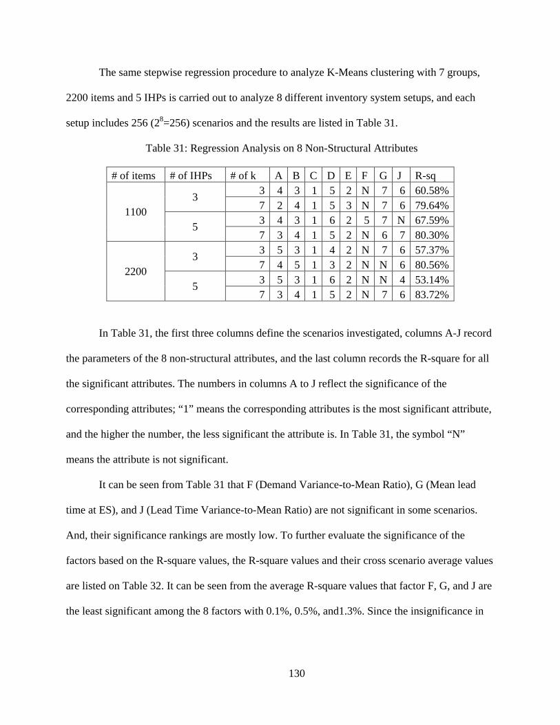
130

The same stepwise regression procedure to analyze K-Means clustering with 7 groups,

2200 items and 5 IHPs is carried out to analyze 8 different inventory system setups, and each

setup includes 256 (28=256) scenarios and the results are listed in Table 31.

Table 31: Regression Analysis on 8 Non-Structural Attributes

# of items # of IHPs # of k A B C D E F G J R-sq

1100 3 3 4 3 1 5 2 N 7 6 60.58%

7 2 4 1 5 3 N 7 6 79.64%

5 3 4 3 1 6 2 5 7 N 67.59% 7 3 4 1 5 2 N 6 7 80.30%

2200 3 3 5 3 1 4 2 N 7 6 57.37%

7 4 5 1 3 2 N N 6 80.56%

5 3 5 3 1 6 2 N N 4 53.14% 7 3 4 1 5 2 N 7 6 83.72%

In Table 31, the first three columns define the scenarios investigated, columns A-J record

the parameters of the 8 non-structural attributes, and the last column records the R-square for all

the significant attributes. The numbers in columns A to J reflect the significance of the

corresponding attributes; “1” means the corresponding attributes is the most significant attribute,

and the higher the number, the less significant the attribute is. In Table 31, the symbol “N”

means the attribute is not significant.

It can be seen from Table 31 that F (Demand Variance-to-Mean Ratio), G (Mean lead

time at ES), and J (Lead Time Variance-to-Mean Ratio) are not significant in some scenarios.

And, their significance rankings are mostly low. To further evaluate the significance of the

factors based on the R-square values, the R-square values and their cross scenario average values

are listed on Table 32. It can be seen from the average R-square values that factor F, G, and J are

the least significant among the 8 factors with 0.1%, 0.5%, and1.3%. Since the insignificance in

131

certain scenarios and the very low corresponding R-square values of these three factors, this

research rules out them from the grouping processes as insignificant attributes.

Table 32: Regression Analysis on 9 Non-Structural Attributes – R-square

# of items

# of locations

# of k A B C D E F G J R-sq

1100

3 3 3.0% 5.2% 39.7% 2.3% 7.0% 0.0% 1.3% 2.1% 60.6% 7 5.6% 3.2% 61.9% 3.0% 4.6% 0.0% 0.5% 0.8% 79.6%

5 3 2.6% 4.8% 46.8% 0.8% 10.9% 1.0% 0.7% 0.0% 67.6% 7 4.9% 3.7% 60.6% 1.2% 9.1% 0.0% 0.6% 0.4% 80.3%

2200

3 3 2.7% 4.0% 33.9% 3.7% 10.5% 0.0% 0.8% 1.8% 57.4% 7 4.3% 3.9% 60.8% 5.2% 5.6% 0.0% 0.0% 0.8% 80.6%

5 3 2.6% 5.9% 29.1% 0.9% 10.7% 0.0% 0.0% 3.9% 52.0% 7 4.7% 4.4% 64.1% 3.2% 6.4% 0.0% 0.3% 0.7% 83.7%

Average 3.8% 4.4% 49.6% 2.5% 8.1% 0.1% 0.5% 1.3% 70.2%

6.3.2 The Tendency of Clustering Same NIT Structures Together

This section deals with Question K2 (whether the item types having the same NIT

structure tend to be clustered into the same group when using Non-Structural attributes?) in

Section 5.1.2.2.

The non-structural attributes are listed in Table 21 with Factor Indices from A to J,

among which C (Ordering Cost), D (Inventory Holding Charge), E (Demand Rate), F (Demand

Variance-to-Mean Ratio) are location related attributes. Location related attributes means when

an item is not stored on a specific location, the corresponding location related attribute value

should not be numerically involved in the grouping process. However, it should be noted that

location related attributes are considered on the locations where the specific item is stored. The

non-structural attributes for K-means clustering method are organized as shown in Exhibit 10,

where all the non-structural attributes on the corresponding locations of the inventory system are

listed (represented). This means that the location related attributes should be involved in the

132

grouping process to reflect the storage status of an item in the inventory network system. As

mentioned in 3.3.2, an item type’s existence at a specific location can be represented using

binary system, i.e. 0 represents non-existence, and 1 existence. Considering the numeric

characteristic of the non-structural attributes involved in the K-means clustering process, the

non-existing non-structural attribute on a specific location needs to be numerically represented.

Therefore, the 0’s representing the non-existence of a specific item on a specific location is

treated as numeric 0 rather than binary 0 in this part of the research. Further, to avoid the

confusion, these numeric 0s are substituted by 0.0001, which is a sufficiently small value that

does not affect the calculation of the grouping performance measures. With all these adjustments,

it should be noted that, following the input structure (representation) of the non-structural

attributes on Exhibit 10, the non-structural attributes all together actually carries storage

structural information by reflecting whether certain items exist on certain locations and by

reflecting the storage networks as whole for the item types. This means that NIT structural

information is put into the clustering process by this way of representation (organization) of the

clustering attribute input values.

From the discussion so far, there are three ways to take the storage structure into

consideration in the clustering process; first is to have binary system represent the storage status

of the item types in the inventory network; second is to use non-structural attributes organized in

the way described in the immediately previous paragraph; and third is to use both first and

second ways together. Considering this section investigates K-means clustering method

characteristics, and the first way is actually the NIT classification process, in this section of the

research the second way is investigated to find out whether the involvement of the storage

structural information in the clustering process using aforementioned non-structural clustering

133

attributes representation evidently affects the clustering results. The third way is the research

topic of next section.

As shown in Exhibit 10, 8 non-structural attributes (factors A to J in the Table 21) are

used in the clustering. And then, statistical analysis is conducted for each resulted cluster to see

whether the items with certain storage structure dominate the entire group. Dominate here means

whether majority of the item types in the same clusters have the same NITs. This is measured by

calculating the percentage of the same NITs in a resulting cluster. Table 33 is an illustration of

the main (dominating) NIT analysis. For group 1, 22 out of total 26 items, which means 85% of

the items, have the storage structure NIT A. Thus, the main NIT for group 1 is NIT A. Similarly,

the main NIT for group 2 is NIT B dominating by 81% as the main structure, and the main NIT

for group 3 is NIT C and 79% of the items in this group have this structure. In this case, the

average percentage of the main structure across the clusters is the average of 85%, 81% and 79%,

which is 81.7%.

Table 33: An Example of Main NIT Analysis

NIT A NIT B NIT C Main Structure % of Main Structure Group 1 22 3 1 NIT A 85 Group 2 3 22 2 NIT B 81 Group 3 3 3 23 NIT C 79

Considering the 5 significant non-structural attributes selected in the previous section and

inventory system setup shown in Table 31, 3-group and 7-group K-means clustering was

implemented to answer whether the item types having the same NIT structure tend to be

clustered into the same group when using significant Non-Structural attributes. The results show

that in 3-group case the across scenario average of % of Main Structure means is 81.3 (variance

69.6), 7-group case the across scenario average of % of Main Structure means is 90.6 (variance

134

56.0). With more than 80% of NITs having the same structure, the results show that the same

NIT tends to be grouped together during the K-Means clustering process. It should also be noted

from the results that when the grouping number increases, the tendency of clustering the same

NIT structures together is more significant.

6.3.3 The Effect of Structural Attributes on the Clustering Results

This section deals with Question K3 (whether the structural attributes affect the

clustering results?) in Section 5.1.2.2 by adding structural attributes into the K-means attribute

list in the clustering process.

The binary expression (illustrated in section 3.3.2 ) is used to represent structural attribute

NIT, i.e., one NIT is represented as a set of binary values, each of which represent the existence

of a retail store at a location. Table 34 records the results of 4 response variables, SSE, %CPC

(the percentage of clustering penalty cost), average percentage of main NIT, and GT (Grouping

Time). Each response in Table 34 is the average value of 1024 (210=1024) scenarios involving

the 10 factors in Table 21.

Table 34: Results for Structural and Non-Structural Attributes

# of Groups SSE(102) %CPC Avg % of Main NIT

GT (0.01secs)

Significant Non-Structural Attributes

3 13.46 10.00 81.27 7.07

Structural and Significant Non-Structural Attributes

3 15.72 11.55 87.19 12.27

Significant Non-Structural Attributes

7 10.43 8.98 90.55 9.80

Structural and Significant Non-Structural Attributes

7 10.64 9.20 96.66 21.77

Figure 46 and Figure 47 show the changes of the four response variables in this

experiment.

135

Figure 46: Comparisons between Significant Non-Structural Attributes and Structural and

Significant Non-Structural Attributes (3-group Case)

Figure 47: Comparisons between Significant Non-Structural Attributes and Structural and

Significant Non-Structural Attributes (7-group Case)

Figure 46 is the comparisons between K-Means clustering using significant non-

structural attributes and clustering using structural and significant non-structural attributes in the

136

3-group case. From Figure 46, it can be seen that adding the structural attributes increase

SSE, %CPC, Avg % of Main NIT, and GT. In addition, Figure 47 is the comparisons between K-

Means clustering using significant non-structural attributes and clustering using structural and

significant non-structural attributes in the 7-group case. This figure also indicates that adding the

structural attributes increases the values of the four responses.

The results show that values of SSE, %CPC, Avg % of Main NIT increase 16.8%, 15.5%,

and 7.3% respectively in 3-group case while the increase on GT is 73.5%, and 2.0%, 2.5%, and

6.7%respectively in 7-group case, while the increase on GT is 122.2%. The increase on %CPC

and SEE shows that the repeated involvement of structural attributes with 0 and 1 values, while

the important non-structural attributes already are carrying the structural information (refer to

Section 6.3.2), causes the unfavorable increase on these performance measures. In other words,

the repeated involvement of the structural attributes in distance calculation in grouping procedure

results larger distance between items, and this affects the grouping results, therefore causes

higher %CPC and SSE. Since the K-means clustering using the significant non-structural

attributes includes the structural information as previously discussed, and the consistent increases

on SSE, %CPC, and Avg % of Main NIT are trivial compared to the increase of GT, for the

reason of experimental efficiency and unfavorable increase on %CPC, SSE, the following

experiments are implemented based on significant non-structural attributes.

6.3.4 The Factors Affecting the K-Means Clustering Time

This section deals with Question K4 (which factors affect the K-Means clustering time?)

in Section 5.1.2.2.

As discussed in Maimon and Rokach (2005), the time complexity of K-Means algorithm

relates to three factors: 1) the number of instances; 2) the number of clusters; and 3) the number

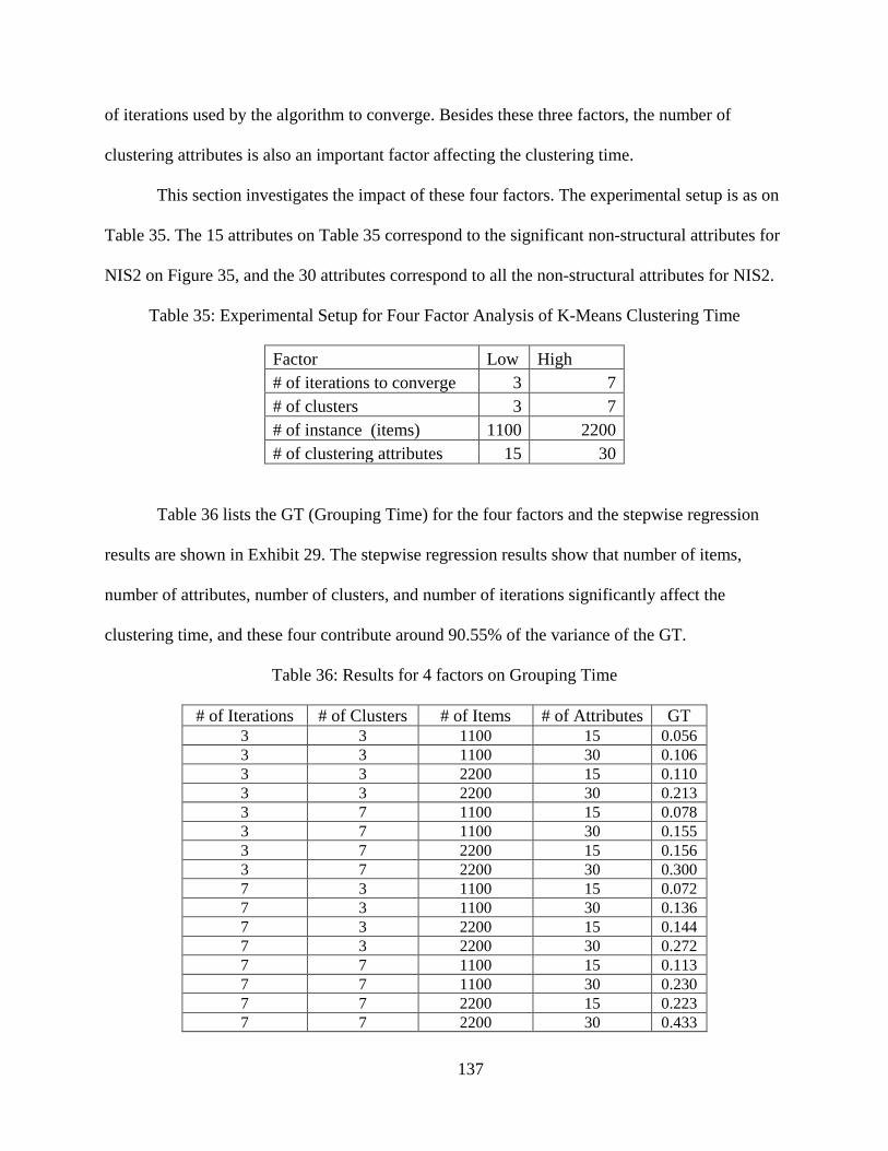
137

of iterations used by the algorithm to converge. Besides these three factors, the number of

clustering attributes is also an important factor affecting the clustering time.

This section investigates the impact of these four factors. The experimental setup is as on

Table 35. The 15 attributes on Table 35 correspond to the significant non-structural attributes for

NIS2 on Figure 35, and the 30 attributes correspond to all the non-structural attributes for NIS2.

Table 35: Experimental Setup for Four Factor Analysis of K-Means Clustering Time

Factor Low High # of iterations to converge 3 7 # of clusters 3 7 # of instance (items) 1100 2200 # of clustering attributes 15 30

Table 36 lists the GT (Grouping Time) for the four factors and the stepwise regression

results are shown in Exhibit 29. The stepwise regression results show that number of items,

number of attributes, number of clusters, and number of iterations significantly affect the

clustering time, and these four contribute around 90.55% of the variance of the GT.

Table 36: Results for 4 factors on Grouping Time

# of Iterations # of Clusters # of Items # of Attributes GT 3 3 1100 15 0.056 3 3 1100 30 0.106 3 3 2200 15 0.110 3 3 2200 30 0.213 3 7 1100 15 0.078 3 7 1100 30 0.155 3 7 2200 15 0.156 3 7 2200 30 0.300 7 3 1100 15 0.072 7 3 1100 30 0.136 7 3 2200 15 0.144 7 3 2200 30 0.272 7 7 1100 15 0.113 7 7 1100 30 0.230 7 7 2200 15 0.223 7 7 2200 30 0.433

138

Stepwise Regression: CT versus iterations, clusters, items, attributes

Stepwise Selection of Terms

Candidate terms: Iterations, Clusters, Items, Attributes

-------Step 1------ -------Step 2------ -------Step 3------

Coef P Coef P Coef P

Constant 0.0050 -0.1624 -0.2529

Items 0.000103 0.017 0.000103 0.002 0.000103 0.000

Attributes 0.00744 0.003 0.00744 0.000

Clusters 0.01811 0.010

Iterations

S 0.0834502 0.0605775 0.0471744

R-sq 34.45% 67.93% 82.05%

R-sq(adj) 29.77% 62.99% 77.56%

R-sq(pred) 14.38% 51.41% 68.08%

Mallows’ Cp 64.30 27.33 12.90

-------Step 4------

Coef P

Constant -0.3232

Items 0.000103 0.000

Attributes 0.00744 0.000

Clusters 0.01811 0.002

Iterations 0.01406 0.009

S 0.0357464

R-sq 90.55%

R-sq(adj) 87.11%

R-sq(pred) 80.01%

Mallows’ Cp 5.00

α to enter = 0.05, α to remove = 0.05 Exhibit 29: Stepwise Regression Analysis on GT based on 4 factors

The R-Squares for the significant factors affecting the grouping time is plotted in Figure

48. The results show that the number of items is the most significant factor which contributes to

34.45% of the R-Squares, the number of clustering attributes is the second significant factor

139

which explains 33.48% of the R-Squares, the number of clusters is the third significant factor

which explains 14.12% of the R-Squares, and the number of iteration for K-Means to converge is

the fourth significant factor which contributes to 8.5% of the R-Squares.

Figure 48: Grouping Time Analysis for Four Factors

6.3.5 The Effect of the Number of Clusters K on the Clustering Results

This section deals with Question K5 (how the number of clusters k affects the clustering

results?) in Section 5.1.2.2.

This experiment is conducted based on two scenarios by comparing the trend on both gap

statistic mentioned in section 3.3.3 and the SSE values for different number of groups. In both

scenarios, the 10 attributes (listed on Table 21) including the structural attributes, non-structural

attributes, and the number of items are used to generate data for the K-Means clustering. For the

1st scenario, all the 10 factors are chosen at their low levels. And for the 2nd scenario, all the 10

factors are chosen at their high levels.

34.45%

33.48%

14.12%

8.50%

9.45%

Grouping Time Analysis for 4 Factors

# of Items# of Attributes# of Clusters# of Iterationsother

140

The maximum number of groups is calculated based on the simple rule of sum (𝑘 ≈

�𝑛/2). In the 2nd scenario, there are 2200 items. Thus, the maximum number of groups is set to

be 33.

The results of the adjusted SSE and gap statistics (refer to Section 3.3.3) are illustrated in

Figure 49 and Figure 50. In these figures, the horizontal axis is number of groups, and the

vertical axis is the % of change of Gap_adj (Adjusted Gap) and SSE_adj (Adjusted SSE). The

original values of SSE are adjusted to the percent ratio of the original value to the maximum SSE,

and the original values of gap statistics are adjusted to the percentage ratio of the original value

to the maximum gap statistic. The purpose of adjusting values of SSE and gap statistics is to see

the trends of SSE and gap statistic in the same figure.

Figure 49: Trend of SSE and Gap Statistics for Scenario 1

141

Figure 50: Trend of SSE and Gap Statistics for Scenario 2

Figure 49 shows that SSE is not monotonically decreasing with k, this may be due to the

randomness of choosing initial seeds; however, its overall trend is decreasing as shown. Also, the

gap statistic is not monotonically increasing; however, its overall trend is increasing. The same

conclusions can be derived based on Figure 50. These trends indicate that in general, the larger

the k value is, the better the clustering results are. This means that in practice, a simple way to

determine k is to fix its values to the largest acceptable value.

6.4 Comparison between Grouping Methods

This section compares the ABC classification, NIT classification, and K-Means

clustering. The comparisons are based on following experimental setups, which are derived

based on previous individual grouping methods related experiments, for the three grouping

methods respectively:

ABC classification:

• NIC is selected as the classification criteria

142

• 7-group classification is selected to implement the comparison with the other

grouping techniques

K-means clustering:

• significant non-structural attributes are selected as the clustering attributes

• 7-group clustering is selected to implement the comparison with the other

grouping techniques

• Number of iteration is set to 3

NIT classification:

• Based on an inventory system with 3 echelon 3 retailers, which allows comparing

NIT with the other grouping methods based on 7 groups

The ABC classification, NIT classification, and K-means clustering methods are

compared based on the following experimental design:

• Number of replication is 1

• Randomized Complete Block Design

The system characteristics used in the experiments are listed on Table 21. To compare the

grouping methods based on 7 groups, the number of IHP is seleceted as 5 (3 echelon 3-retailer

case). The other 9 attributes listed on Table 21 takes 2 levels as shown on the table. This way,

there are 512 (29=512) system scenarios considered on each comparison experiment. The

experiments implement Randomized Complete Block Design. Each block in this case represents

one scenario. A complete block is an experimental setup that tests the three methods by putting

them in one scenario. The randomization is implemented by randomizing the sequence of the

experiments corresponding to each of the grouping methods within each block. Following are the

hypothesis and the corresponding statistical analysis.

143

Experiment based on %CPC

The hypothesis of comparing the three grouping methods:

H0: µ1 = µ2 = µ3 (% CPC does not change for the three grouping methods)

H1: µ1 ≠ µ2 ≠µ3 (% CPC for the three different grouping methods are different)

(µ1: mean of %CPC for ABC; µ2: mean of %CPC for NIT; mean of %CPC for K-means;

α=0.05)

ANOVA is used to compare the means of %CPC for the three grouping methods, and the results

are on Exhibit 30. It can be seen from Exhibit 30 that the Null hypothesis is rejected (P-value =

0,000), which means that %CPC changes for the three grouping methods. Since the null

hypothesis is rejected in the ANOVA, it can be concluded that some of the factor level means are

different. Considering ANOVA does not identify which means are different, Fisher’s least

significant difference (LSD) method as the multiple comparisons method is implemented to

compare the three methods.

The result of Fisher’s LSD is on Figure 51. The comparison results show that K-means, NIT, and

ABC grouping methods have significant differences respect to %CPC. It can be seen that K-

means clustering out performs both NIT and ABC classifications, while NIT grouping performs

better than ABC classification.

One-way ANOVA: %CPC versus Grouping Method

Method

Null hypothesis All means are equal

Alternative hypothesis At least one mean is different

Significance level α = 0.05 Equal variances were assumed for the analysis.

Factor Information

Factor Levels Values

Grouping Method 3 ABC, K-Means, NIT

144

Analysis of Variance

Source DF Adj SS Adj MS F-Value P-Value

Grouping Method 2 5426 2712.76 2307.90 0.000

Error 1533 1802 1.18

Total 1535 7227

Model Summary

S R-sq R-sq(adj) R-sq(pred)

1.08417 75.07% 75.04% 74.97%

Means

Grouping

Method N Mean StDev 95% CI

ABC 512 12.9424 1.0840 (12.8484, 13.0364)

K-Means 512 8.7984 1.0283 ( 8.7045, 8.8924)

NIT 512 12.6070 1.1375 (12.5130, 12.7010)

Pooled StDev = 1.08417

Fisher Pairwise Comparisons

Grouping Information Using the Fisher LSD Method and 95% Confidence

Grouping

Method N Mean Grouping

ABC 512 12.9424 A

NIT 512 12.6070 B

K-Means 512 8.7984 C

Means that do not share a letter are significantly different.

Fisher Individual Tests for Differences of Means

Difference of Difference SE of Adjusted

Levels of Means Difference 95% CI T-Value P-Value

K-Means - ABC -4.1439 0.0678 (-4.2769, -4.0110) -61.16 0.000

NIT - ABC -0.3354 0.0678 (-0.4683, -0.2024) -4.95 0.000

NIT - K-Means 3.8086 0.0678 ( 3.6757, 3.9415) 56.21 0.000

Simultaneous confidence level = 87.81%

Exhibit 30: Minitab Analysis of Variance Output for %CPC

145

Figure 51: Fisher’s Pairwise Comparisons for % CPC

Experiment based on SSE

The hypothesis of comparing the three grouping methods:

H0: µ1 = µ2 = µ3 (SSE does not change for the three grouping methods)

H1: µ1 ≠ µ2 ≠µ3 (SSE for the three different grouping methods are different)

(µ1: mean of SSE for ABC; µ2: mean of SSE for NIT; mean of SSE for K-means; α=0.05)

It can be seen from Exhibit 31 that the Null hypothesis is rejected (P-value = 0,000),

which means that SSE changes for the three grouping methods. Since the null hypothesis is

rejected in the ANOVA, it can be concluded that some of the factor level means are different.

The result of Fisher’s LSD is on Figure 52. The comparison results show that K-means,

NIT, and ABC grouping methods have significant differences respect to SSE. It can be seen that

146

K-means clustering out performs both NIT and ABC classifications, while NIT grouping

performs better than ABC classification.

One-way ANOVA: SSE versus Grouping Method

Method

Null hypothesis All means are equal

Alternative hypothesis At least one mean is different

Significance level α = 0.05 Equal variances were assumed for the analysis.

Factor Information

Factor Levels Values

Grouping Method 3 ABC, K-Means, NIT

Analysis of Variance

Source DF Adj SS Adj MS F-Value P-Value

Grouping Method 2 649503647 324751824 559.15 0.000

Error 1533 890366386 580800

Total 1535 1539870033

Model Summary

S R-sq R-sq(adj) R-sq(pred)

762.102 42.18% 42.10% 41.95%

Means

Grouping

Method N Mean StDev 95% CI

ABC 512 2954.9 969.4 (2888.8, 3020.9)

K-Means 512 1372.5 466.3 (1306.4, 1438.6)

NIT 512 2321.5 764.9 (2255.4, 2387.5)

Pooled StDev = 762.102

Fisher Pairwise Comparisons

Grouping Information Using the Fisher LSD Method and 95% Confidence

Grouping

Method N Mean Grouping

ABC 512 2954.9 A

147

NIT 512 2321.5 B

K-Means 512 1372.5 C

Means that do not share a letter are significantly different.

Fisher Individual Tests for Differences of Means

Difference of Difference SE of Adjusted

Levels of Means Difference 95% CI T-Value P-Value

K-Means - ABC -1582.4 47.6 (-1675.8, -1488.9) -33.22 0.000

NIT - ABC -633.4 47.6 ( -726.8, -540.0) -13.30 0.000

NIT - K-Means 949.0 47.6 ( 855.6, 1042.4) 19.92 0.000

Simultaneous confidence level = 87.81%

Exhibit 31: Minitab Analysis of Variance Output for SSE

Figure 52: Fisher’s Pairwise Comparisons for SSE

Experiment based on GT

The hypothesis of comparing the three grouping methods:

H0: µ1 = µ2 = µ3 (GT does not change for the three grouping methods)

H1: µ1 ≠ µ2 ≠µ3 (GT for the three different grouping methods are different)

(µ1: mean of GT for ABC; µ2: mean of GT for NIT; mean of GT for K-means; α=0.05)

148

It can be seen from Exhibit 32 that the Null hypothesis is rejected (P-value = 0,000),

which means that GT changes for the three grouping methods. Since the null hypothesis is

rejected in the ANOVA, it can be concluded that some of the factor level means are different.

The result of Fisher’s LSD is on Figure 53. The comparison results show that K-means

have significant difference with NIT and ABC grouping methods respect to GT, while NIT and

ABC do not have significant difference. It can be seen that K-means takes longer clustering time

than both NIT and ABC classifications.

One-way ANOVA: GT versus Grouping Method

Method

Null hypothesis All means are equal

Alternative hypothesis At least one mean is different

Significance level α = 0.05 Equal variances were assumed for the analysis.

Factor Information

Factor Levels Values

Grouping Method 3 ABC, K-Means, NIT

Analysis of Variance

Source DF Adj SS Adj MS F-Value P-Value

Grouping Method 2 0.2185 0.109264 68.49 0.000

Error 1533 2.4455 0.001595

Total 1535 2.6640

Model Summary

S R-sq R-sq(adj) R-sq(pred)

0.0399405 8.20% 8.08% 7.84%

Means

Grouping

Method N Mean StDev 95% CI

ABC 512 0.09046 0.04480 (0.08699, 0.09392)

K-Means 512 0.11520 0.03902 (0.11174, 0.11866)

NIT 512 0.08937 0.03545 (0.08591, 0.09284)

Pooled StDev = 0.0399405

149

Fisher Pairwise Comparisons

Grouping Information Using the Fisher LSD Method and 95% Confidence

Grouping

Method N Mean Grouping

K-Means 512 0.11520 A

ABC 512 0.09046 B

NIT 512 0.08937 B

Means that do not share a letter are significantly different.

Fisher Individual Tests for Differences of Means

Difference of Difference SE of Adjusted

Levels of Means Difference 95% CI T-Value P-Value

K-Means - ABC 0.02474 0.00250 ( 0.01985, 0.02964) 9.91 0.000

NIT - ABC -0.00108 0.00250 (-0.00598, 0.00381) -0.43 0.665

NIT - K-Means -0.02583 0.00250 (-0.03072, -0.02093) -10.35 0.000

Simultaneous confidence level = 87.81%

Exhibit 32: Minitab Analysis of Variance Output for GT

Figure 53: Fisher’s Pairwise Comparisons for GT

150

6.5 Conclusions on the Grouping Methods

The experimental results regarding the grouping methods can be summarized as

following:

ABC classification

• NIC as the classification criteria out performs NADU regarding to both %CPC

and GT

• 7-group classification is significantly better than 3-group case according

to %CPC values, and the resulted GT shows there is no significant difference

between 7-group and 3-group cases

K-means Clustering

• The significant non-structural attributes identified in this research are Unit Cost,

Lost-Sale-Cost-to-Unit-Cost Ratio, Ordering Cost, Inventory Holding Charge,

Demand Rate

• Structural information can be put in the K-means algorithm by identifying and

representing location related attribute values to form clusters that having

structural within group similarity

• After considering location related attributes in the K-means clustering, there is no

need to add structural attributes represented in binary values

• Among the four factors that affect the GT, the number of items is the most

significant factor, the number of clustering attributes is the second significant

factor, the number of clusters is the third significant factor, and the number of

iteration for K-Means to converge is the fourth significant factor

• In general, the larger the k value is, the better the clustering results are

151

Comparison between the Three Grouping Techniques

• Based on %CPC and SSE, K-means clustering out performs both NIT and ABC

classifications, while NIT grouping performs better than ABC classification

• Based on GT, K-means takes longer clustering time than both NIT and ABC

classifications, while there is no significant difference between NIT and ABC

152

7 Summary

This chapter discusses the conclusions, suggestions, and future work.

7.1 Conclusions

The main focus of this research is to investigate the grouping techniques for large scale

multi-item multi-echelon inventory system. The whole research is driven by six main research

questions (Q1 to Q6) discussed in the introduction chapter.

The 1st research question is about the representation of the inventory system of interest

and the inventory items to facilitate analysis and implementation of grouping methods. In order

to deal with this question, the characteristics of the inventory items are categorized as structural

and non-structural attributes. The most important structural attribute is the network of item type

(NIT) which demonstrates the storage structure of an item. This attribute can be including in the

grouping process either by represented using binary system (in NIT classification and K-means

clustering), or in the way of organizing the grouping attributes listed in Exhibit 10. Involving the

NIT by representing it using binary system in K-means clustering is not suggested based on the

corresponding experimental results. This research is the first study that models the structural

attribute of an item using its supply network, or put it in other words, using the network of item

type (NIT). In section 3.3.2, the NIT is modeled using graph theory representation (binary

expression). Compared to ABC classification and K-Means clustering, the experimental results

show that the NIT classification using binary expression uses the shortest time to group large

number of items. The non-structural attributes are modeled as continuous decimal values to

calculate the Euclidean distance between items.

The 2nd research question is about the data generation method. A multi-item multi-

echelon (MIME) data generation procedure is developed to generate different datasets

153

representing a variety of large scale inventory systems. The inputs of the data generation are user

configurable, so that controllable large scale MIME inventory system datasets are generated.

This helps the experiments and facilitates the testing of the grouping methods. The data

generation procedure is designed using the Java Classes developed in the process of dealing with

1st research question. It is believed that this dissertation is the first research that uses the NIT for

data generation. As illustrated in Section 4.2.2.2, the structural attribute NIT facilitates the

generation of SKUs and demands in the data generation process for the large scale inventory

system of interest. To make the generated dataset more realistic, six directly related papers are

studied to determine the range of data generation inputs, and a procedure involving a sequence of

conditional probability distributions suggested by Rossetti and Achlerkar (2011) is used to

satisfy the direct or inverse proportional relationships between a pair of input attributes.

The 3rd research question is about which system and item characteristics should be used

in the grouping process. The answer to this question depends on the grouping method. For ABC

classification, the characteristics that are involved in the classification criterion participate in the

grouping process. For NIT classification, the structural attribute NIT is used for separating the

items. For K-Means clustering, the characteristics that involved in the cost model are used as the

clustering attributes. As discussed in Section 6.3, not all system and item characteristics that are

involved in the cost model significantly affect the clustering results. Also, the experimental

results show that including structural attributes in the K-Means clustering attributes increase

clustering penalty cost and consumes more clustering time. Thus, structural attributes are not

suggested to be directly involved in the K-Means clustering.

The 4th research question related investigation deals with the importance-based

classification from the network perspective. This research question also relates to the question

154

A1 and A2 discussed in Section 4.2.4.4 and 6.2. This dissertation discusses the process of

selecting appropriate ABC classification criterion by reviewing Zhang et al. (2001) and Teunter

et al. (2010), and summarizes the rules of selecting/developing classification criterion. Based on

the summarized rules, two network-based classification criteria are developed. The 1st

classification criterion, the network inventory cost (NIC), which is shown in Equation (13) of

Section 3.3.1, is developed based on Hadley and Whitin (1963)’s Model to calculate the

inventory cost of the entire network. The 2nd classification criterion, the network annual dollar

usage (NADU), is the sum of traditionally applied annual dollar usage of an item in the entire

inventory network. The purpose of the 2nd classification criterion is to evaluate the new

classification criterion NIC. Two paired-t tests are implemented to compare the effectiveness and

efficiency of NIC and NADU. The measurement for effectiveness is the clustering penalty cost

and the measurement for efficiency is the grouping time. The results show that NIC is

significantly better than NADU from both effectiveness and efficiency perspectives. Also, the

experimental results show that compared to 3 groups, using 7 groups results in smaller clustering

penalty cost.

The 5th research question relates to K-Means clustering. According to Maimon and

Rokach (2005), only K-Means clustering and its equivalent have been successfully applied to

grouping large scale datasets. In order to understand the performance of the K-Means clustering

for the large scale inventory system of interest, five K-Means related research questions (K1 to

K5) are investigated in Section 6.3. The experimental results lead to following suggestions: 1)

structural attributes should not be involved as the clustering attributes in K-Means clustering; 2)

the simplest way to determine k is to set its value to the maximum allowed value; 3) number of

items, number of clustering attributes, number of clusters, and number of iterations significantly

155

affect the clustering time; and 4) items having the same NIT structure tend to be clustered into

the same group.

7.2 Suggestions on Combining the Grouping Techniques in Practice

Individually, ABC classification, NIT classification, and K-Means clustering have their

own unique advantages and disadvantages. This validates Ratliff and Nulty (1997)’s view of

“there is no single best approach, best representation, best model, or best algorithm for

optimizing logistics decisions”. This indicates that it is reasonable to explore the ways to

combine these techniques so that they can be used to their best advantages while avoiding their

disadvantages in practice. It should be also noted from the analysis in the previous section that

the sequence of applying these importance-based classifications and operation-based clustering

may affect the grouping results and practical meaning of the groups. This could lead to different

inventory management strategies in practice. In the following, the possible ways of integrating

classification and clustering techniques are discussed in the context of two stage grouping and

three stage grouping.

ABC Classification + K-Means Clustering

When individually used, ABC classification as an importance-based grouping technique

identifies the important item types in the entire inventory system. It helps management to

prioritize the items according to their importance for the management and financial resources

allocation, so that the inventory items can be managed more effectively. When individually

implemented, K-means clustering as an operational-attributes-based clustering technique groups

together items with similar (close) characteristics from the operational perspective; this

facilitates the implementation of inventory control policy so that lower penalty cost and higher

156

service level can be achieved effectively. These techniques can be combined sequentially

according to the management goal.

If the grouping is carried out in the sequence of the ABC classification first and then the

K-Means clustering, the items will be grouped into 3 or 7 groups first that are prioritized

according to the importance of the item types; in this way, each item is labeled as A item, B item,

or C item indicating their importance. Then, using K-Means clustering, each resulting group

from first step is further divided into item groups based on the operational-attributes; this

facilitates determining the optimal group policy for the items while making the importance of the

items identifiable. This combination of network-based ABC classification and K-Means

clustering extends the traditional single-location-based ABC classification to the network-based

and cost model involved grouping level.

If the grouping is carried out in the sequence of the K-Means clustering first and then the

ABC classification, the items will firstly be grouped into operational groups, each of which holds

item types with similar operational characteristics. In this way, the number of item groups is not

restricted to 3 or 7 at the first stage. Further, classifying each of these operational groups using

the ABC classification developed in this research labels the items in each group according to

their importance to the management. This combination of network-based K-Means clustering

and ABC classification extends the K-Means clustering to item importance involved grouping

level.

NIT Classification + K-Means Clustering

As mentioned previously, as a classification technique based on the storage structure

attribute, NIT classification makes it possible to group the items in such a way that the items in

the same group share exactly the same storage structure. This corresponds to Lenard and Roy

157

(1995)’s suggestion that the differences between the storage structure of items prevent the items

being grouped together for the function of the warehouse is different at different echelons.

If the grouping is implemented in the sequence of the NIT classification first and then the

K-Means clustering, the items with identical storage structures are grouped together first, and

then the resulting item groups are further divided into groups based on the operation-based

attributes. This facilitates the group inventory policy calculation for the items with the same

structural attributes. The ultimate groups will strictly have their own identical structures.

If the grouping is implemented in the sequence of the K-Means clustering first and then

the NIT Classification, the resulted ultimate groups will also strictly have their own identical

structures.

NIT Classification + ABC Classification

The items grouped together using NIT classification and ABC classification sequentially

share the same storage structure and have the importance labels such as A, B, or C. Grouping

first using NIT classification and then ABC classification helps prioritizing the items having the

same storage structure by determining the importance of the items. On the other hand, grouping

first using ABC classification and then NIT classification helps with identifying the storage

structure of items with the same importance (priority); in other words, it helps to group the items

with the same importance and same structure together.

ABC Classification +NIT Classification + K-Means Clustering

A three stage grouping that combine all the three grouping techniques introduced so far in

this research sequentially can result in groups with more complete involvement of the system

characteristics, which may be very favorable in some cases in practice. There are 6 ways of

combination for these methods, and they would result different final groups. It should be noted

158

that no matter in which sequences the grouping is implemented using these three grouping

techniques together, the final resulted groups will have their own unique storage structure due to

the involvement of NIT in the grouping process; they will have importance labels for each item

type included; and they will have operational-attributes with similar (close) values. The diversity

of the resulting groups from applying different sequences in the grouping process provides a

means of investigating a wide variety of clustering scenarios.

The different grouping techniques have their own advantages according to the

management goal. From the three aspects of resulted groups, whether importance of items are

identified, whether have same structure, whether have similar operations-related attributes, the 7

grouping techniques can be compared as in Table 37.

Table 37: Characteristics of the 7 Grouping Techniques

Grouping Method Identifying Important Items

Having Same Structure

Having Similar Operations-Related Attributes

K-Means

Yes ABC Yes

NIT

Yes ABC+ K-Means Yes

Yes

NIT+K-Means

Yes Yes NIT+ABC Yes Yes ABC+NIT+K-Means Yes Yes

Yes

7.3 Future Work

For grouping techniques, there are still many aspects need to be investigated. This section

recommends three aspects to further investigate.

One of the five main factor categories affecting the grouping results is the cost model.

The future research can use the cost model applied by the companies to test the performance of

the network based ABC classification, NIT classification and K-Means clustering, and select the

159

most appropriate grouping method or a combination of grouping methods. The cost model

applied by the companies can be further investigated based on the methodologies developed in

this research.

From the NIT perspective, the NIT modeling can be further investigated and applied to

more realistic scenarios when industrial data is available. Currently, there are several

assumptions about NIT modeling, such as each customer location has only one supply location.

These assumptions may be relaxed after analyzing the characteristics of the storage structures in

the industry. In this research, NIT is studied based on inventory control related activities. NIT

can be investigated to integrate the inventory control, transportation and warehousing activities.

For K-Means clustering technique, the quality of the clustering results relates to the

selection of initial seeds. This research did not investigate this field. The knowledge gained from

the industry could help set up some rules for the selection of initial seeds, which are the centroids

of each group setup in the Initialization Step in Exhibit 14. In addition, industrial instances could

provide some insights into the clustering attributes selection, choosing optimal number of groups,

etc.

160

References

Al-Sultan, K. S., & Khan, M. M. (1996). Computational experience on four algorithms for the hard clustering problem. Pattern Recognition Letters, 17(3), 295-308.

Axsäter, S. (2006). Inventory control (international series in operations research & management

science). Springer, Berlin. Bonner, R. E. (1964). On some clustering techniques. IBM journal of research and development,

8(1), 22-32.. Chaharsooghi, S. K., & Heydari, J. (2010). LT variance or LT mean reduction in supply chain

management: Which one has a higher impact on SC performance?. International Journal of Production Economics, 124(2), 475-481.

Codd, E. F. (1970). A relational model of data for large shared data banks. Communications of

the ACM 13(6), 377–387. Cohen, M. A., Kleindorfer, P. R., & Lee, H. L. (1986). Optimal stocking policies for low usage

items in multi‐echelon inventory systems. Naval Research Logistics Quarterly, 33(1), 17-38.

Cohen, M., and R. Ernst (1988). Multi-item classification and generic inventory stock control

policies. Production and Inventory Management Journal 29 (3), 6–8. Deshpande, V., Cohen, M. A., & Donohue, K. (2003). An empirical study of service

differentiation for weapon system service parts. Operations Research, 51(4), 518-530. Ehrhardt, R. (1984). (s, S) policies for a dynamic inventory model with stochastic lead times.

Operations Research, 32(1), 121-132. Ernst, R., & Cohen, M. A. (1990). Operations related groups (ORGs): a clustering procedure for

production/inventory systems. Journal of Operations Management, 9(4), 574-598. Flores, B. E., & Clay Whybark, D. (1986). Multiple criteria ABC analysis. International Journal

of Operations & Production Management, 6(3), 38-46. Flores, B. E., Olson, D. L., & Dorai, V. K. (1992). Management of multicriteria inventory

classification. Mathematical and Computer modelling, 16(12), 71-82. Guvenir, H. A., & Erel, E. (1998). Multicriteria inventory classification using a genetic

algorithm. European journal of operational research, 105(1), 29-37. Hadley, G., & Whitin, T. M. (1963). Analysis of inventory systems. Englewood Cliffs, N.J:

Prentice-Hall.

161

Hopp, W. J., Spearman, M. L., & Zhang, R. Q. (1997). Easily implementable inventory control policies. Operations Research, 45(3), 327-340.

Hopp, W. J., & Spearman, M. L. (2001) Factory Physics: Foundations of Manufacturing

Management. New York: Irwin-McGraw-Hill. Van Kampen, T. J., Akkerman, R., & Pieter van Donk, D. (2012). SKU classification: a literature

review and conceptual framework. International Journal of Operations & Production Management, 32(7), 850-876.

Lee, H. L., Padmanabhan, V., & Whang, S. (1997). The bullwhip effect in supply chains. MIT

Sloan Management Review, 38(3), 93. Lenard, J. D., & Roy, B. (1995). Multi-item inventory control: A multicriteria view. European

Journal of Operational Research, 87(3), 685-692. MacKay, D. J. C. (2003). Information theory, inference, and learning algorithms. Cambridge,

UK: Cambridge University Press. Montgomery, D. C. (2001). Design and analysis of experiments. New York: John Wiley. Montgomery, D. C., & Runger, G. C. (2003). Applied statistics and probability for engineers.

John Wiley & Sons. Maimon, O., & Rokach, L. (Eds.). (2005). Data mining and knowledge discovery handbook (Vol.

2). New York: Springer. Metters, R. (1997). Quantifying the bullwhip effect in supply chains. Journal of operations

management, 15(2), 89-100. Nahmias, S. (1997). Production and operations analysis. Chicago: Irwin. Ramanathan, R. (2006). ABC inventory classification with multiple-criteria using weighted

linear optimization. Computers & Operations Research 33(3), 695–700. Rumbaugh, J., Blaha, M., Premerlani, W., Eddy, F., & Lorensen, W. E. (1991). Object-oriented

modeling and design (Vol. 199, No. 1). Englewood Cliffs, NJ: Prentice-hall. Ratliff, H. D., & Nulty, W. G. (1997). Logistics composite modeling. In The planning and

scheduling of production systems (pp. 10-53). Springer US. REM ASSOCIATES, R. (n.d.). Methodology of Calculating Inventory Carrying Costs. Retrieved

August 6, 2013, from http://www.remassoc.com/portals/0/remprecc.pdf Romesburg, H.C. (1984) Cluster Analysis for Researchers, 1st ed., Lifetime Learning

Publications, California.

162

Rossetti, M. D., & Achlerkar, A. V. (2011). Evaluation of segmentation techniques for inventory

management in large scale multi-item inventory systems. International Journal of Logistics Systems and Management, 8(4), 403-424.

Rossetti, M. D., & Chen, Y. (2012, December). A cloud computing architecture for supply chain

network simulation. In Proceedings of the 2012 Winter Simulation Conference (WSC) (pp. 1-12). IEEE.

Silverston, L., Inmon, W. H., & Graziano, K. (1997). The data model resource book: a library of

logical data models and data warehouse designs. John Wiley & Sons, Inc.. Silver, E. A., Pyke, D. F., & Peterson, R. (1998). Inventory management and production

planning and scheduling (Vol. 3, p. 30). New York: Wiley. Tan, P., M. Steinbach, V. Kumar, et al. (2006). Introduction to data mining. Pearson Addison

Wesley Boston. Teunter, R. H., Babai, M. Z., & Syntetos, A. A. (2010). ABC classification: service levels and

inventory costs. Production and Operations Management, 19(3), 343-352. Tibshirani, R., Walther, G., & Hastie, T. (2001). Estimating the number of clusters in a data set

via the gap statistic. Journal of the Royal Statistical Society: Series B (Statistical Methodology), 63(2), 411-423.

West, M. (2011). Developing high quality data models. Elsevier. Xu, Z., Ke, Y., Wang, Y., Cheng, H., & Cheng, J. (2012, May). A model-based approach to

attributed graph clustering. In Proceedings of the 2012 ACM SIGMOD International Conference on Management of Data (pp. 505-516). ACM.

Zhang, R. Q., Hopp, W. J., & Supatgiat, C. (2001). Spreadsheet implementable inventory control

for a distribution center. Journal of Heuristics, 7(2), 185-203. Zheng, Y. S. (1992). On properties of stochastic inventory systems. Management science, 38(1),

87-103. Zhou, Y., Cheng, H., & Yu, J. X. (2009). Graph clustering based on structural/attribute

similarities. Proceedings of the VLDB Endowment, 2(1), 718-729.

163

Appendix 1: A Case Study of the Multi-Echelon Inventory Cost Model

In this appendix, using a small instance, the cost model is illustrated by setting the

optimal policies for a single-item two-echelon inventory system. As shown in Figure 54,

consider a warehouse located at echelon 1 that supplies two retail stores at echelon 2.

Figure 54: Multi-Echelon Inventory Cost Model Example

The continuous reorder point reorder quantity policy is used for this two echelon

inventory system. The data used to calculate the cost are listed as follows:

𝐼 ≡ unit cost = 100 dollars

𝑏 = lost sales cost = 50 dollars

𝐴1 ≡ ordering cost at location 3 = 500 dollars

𝐴2 ≡ ordering cost at location 2 = 200 dollars

𝐴3 ≡ ordering cost at location 3 = 300 dollars

𝐼1 ≡ inventory holding charge at location 1 = 0.15 $/$/unit/year

𝐼2 ≡ inventory holding charge at location 2 = 0.2 $/$/unit/year

𝐼3 ≡ inventory holding charge at location 2 = 0.25 $/$/unit/year

𝜆2 ≡ demand rate at location 2 = 1500 𝑑𝑛𝑖𝑖𝑖/𝑃𝑖𝑙𝑟

𝜎𝐷_2 ≡ standard deviation of demand at location 2 = 20 units/year

𝜆3 ≡ demand rate at location 3 = 2000 units/year

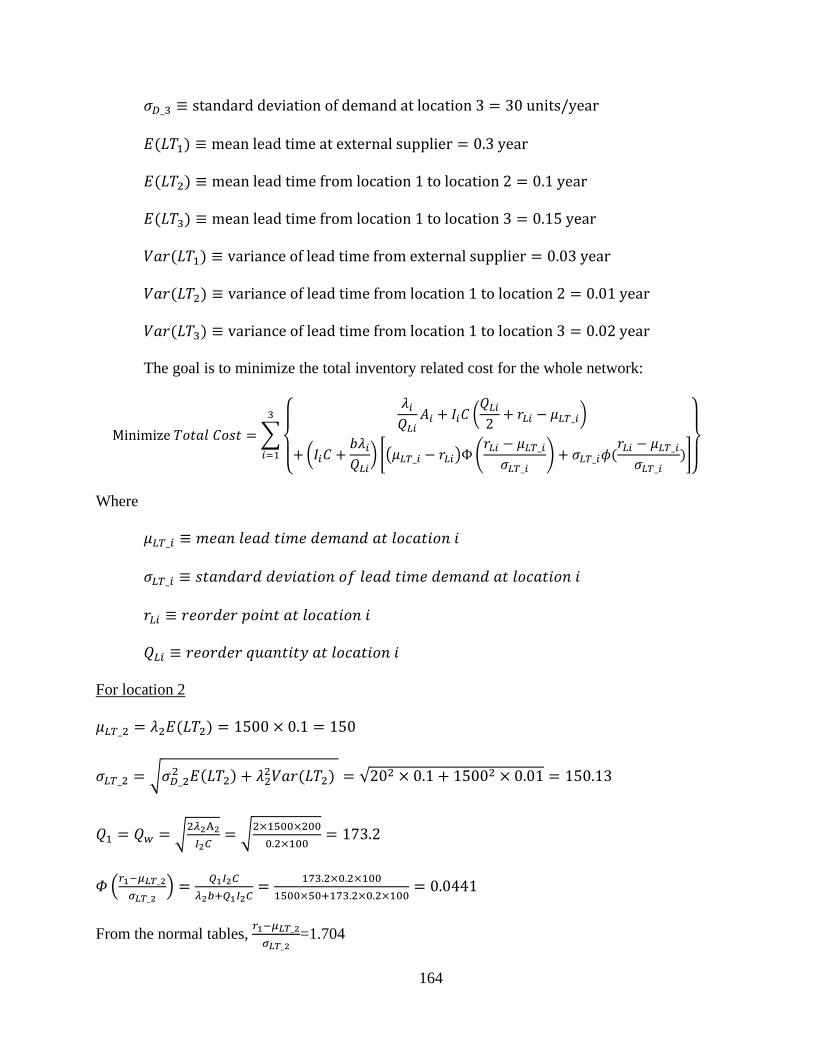
164

𝜎𝐷_3 ≡ standard deviation of demand at location 3 = 30 units/year

𝐸(𝐶𝐺1) ≡ mean lead time at external supplier = 0.3 year

𝐸(𝐶𝐺2) ≡ mean lead time from location 1 to location 2 = 0.1 year

𝐸(𝐶𝐺3) ≡ mean lead time from location 1 to location 3 = 0.15 year

𝑉𝑙𝑟(𝐶𝐺1) ≡ variance of lead time from external supplier = 0.03 year

𝑉𝑙𝑟(𝐶𝐺2) ≡ variance of lead time from location 1 to location 2 = 0.01 year

𝑉𝑙𝑟(𝐶𝐺3) ≡ variance of lead time from location 1 to location 3 = 0.02 year

The goal is to minimize the total inventory related cost for the whole network:

Minimize 𝐺𝑐𝑖𝑙𝑙 𝐼𝑐𝑖𝑖 = �

⎩⎪⎨

⎪⎧ 𝜆𝑖

𝑄𝐿𝑖𝐴𝑖 + 𝐼𝑖𝐼 �

𝑄𝐿𝑖2

+ 𝑟𝐿𝑖 − 𝜇𝐿𝐿_𝑖�

+ �𝐼𝑖𝐼 +𝑏𝜆𝑖𝑄𝐿𝑖

� ��𝜇𝐿𝐿_𝑖 − 𝑟𝐿𝑖�Φ�𝑟𝐿𝑖 − 𝜇𝐿𝐿_𝑖

𝜎𝐿𝐿_𝑖� + 𝜎𝐿𝐿_𝑖𝜙(

𝑟𝐿𝑖 − 𝜇𝐿𝐿_𝑖

𝜎𝐿𝐿_𝑖)�⎭⎪⎬

⎪⎫3

𝑖=1

Where

𝜇𝐿𝐿_𝑖 ≡ 𝑚𝑖𝑙𝑛 𝑙𝑖𝑙𝑑 𝑖𝑖𝑚𝑖 𝑑𝑖𝑚𝑙𝑛𝑑 𝑙𝑖 𝑙𝑐𝑐𝑙𝑖𝑖𝑐𝑛 𝑖

𝜎𝐿𝐿_𝑖 ≡ 𝑖𝑖𝑙𝑛𝑑𝑙𝑟𝑑 𝑑𝑖𝐼𝑖𝑙𝑖𝑖𝑐𝑛 𝑐𝑎 𝑙𝑖𝑙𝑑 𝑖𝑖𝑚𝑖 𝑑𝑖𝑚𝑙𝑛𝑑 𝑙𝑖 𝑙𝑐𝑐𝑙𝑖𝑖𝑐𝑛 𝑖

𝑟𝐿𝑖 ≡ 𝑟𝑖𝑐𝑟𝑑𝑖𝑟 𝑝𝑐𝑖𝑛𝑖 𝑙𝑖 𝑙𝑐𝑐𝑙𝑖𝑖𝑐𝑛 𝑖

𝑄𝐿𝑖 ≡ 𝑟𝑖𝑐𝑟𝑑𝑖𝑟 𝑞𝑑𝑙𝑛𝑖𝑖𝑖𝑃 𝑙𝑖 𝑙𝑐𝑐𝑙𝑖𝑖𝑐𝑛 𝑖

For location 2

𝜇𝐿𝐿_2 = 𝜆2𝐸(𝐶𝐺2) = 1500 × 0.1 = 150

𝜎𝐿𝐿_2 = �𝜎𝐷_22 𝐸(𝐶𝐺2) + 𝜆22𝑉𝑙𝑟(𝐶𝐺2) = √202 × 0.1 + 15002 × 0.01 = 150.13

𝑄1 = 𝑄𝑤 = �2𝜆2A2𝐼2𝐼

= �2×1500×2000.2×100

= 173.2

𝛷 �𝑟1−𝜇𝐿𝐿_2𝜎𝐿𝐿_2

� = 𝑄1𝐼2𝐼𝜆2𝑏+𝑄1𝐼2𝐼

= 173.2×0.2×1001500×50+173.2×0.2×100

= 0.0441

From the normal tables, 𝑟1−𝜇𝐿𝐿_2𝜎𝐿𝐿_2

=1.704

165

𝑟1 = 1.704 × 𝜎𝐿𝐿_2 + 𝜇𝐿𝐿_2 = 1.704 × 150.13 + 150 = 405.82

𝜙 �𝑟1−𝜇𝐿𝐿_2𝜎𝐿𝐿_2

� = 𝜙(1.704) = 0.0933

𝜂(𝑟1) = �𝜇𝐿𝐿_2 − 𝑟1�𝛷 �𝑟1−𝜇𝐿𝐿_2𝜎𝐿𝐿_2

� + 𝜎𝐿𝐿2𝜙 �𝑟1−𝜇𝐿𝐿_2𝜎𝐿𝐿_2

�

= (150 − 405.82) ∗ 0.0441 + 150.13 ∗ 0.0933 =2.7254

𝑄2 = �2𝜆2[𝐴2+𝑏∗𝜂(𝑟1)]𝐼2𝐼

= �2×1500×[200+50×2.7254]0.2×100

= 224.59

𝛷 �𝑟2−𝜇𝐿𝐿_2𝜎𝐿𝐿_2

� = 𝑄2𝐼2𝐼𝜆2𝑏+𝑄2𝐼2𝐼

= 224.59×0.2×1001500×50+224.59×0.2×100

= 0.0565

From the normal tables, 𝑟2−𝜇𝐿𝐿_2𝜎𝐿𝐿_2

=1.579

𝑟2 = 1.579 × 𝜎𝐿𝐿_2 + 𝜇𝐿𝐿_2 = 1.579 × 150.13 + 150 = 387.05

Then, the stop criterion is checked. In this example, the stop criterion is 𝑟1−𝑟2𝑟1

≤ 0.02.

Since 𝑟1−𝑟2𝑟1

= 405.82−387.05405.82

= 0.046 > 0.02, continue to search the optimal solution.

𝜙 �𝑟2−𝜇𝐿𝐿_2𝜎𝐿𝐿_2

� = 𝜙(1.579) = 0.1147

𝜂(𝑟2) = �𝜇𝐿𝐿_2 − 𝑟2�𝛷 �𝑟2−𝜇𝐿𝐿_2𝜎𝐿𝐿_2

� + 𝜎𝐿𝐿_2𝜙 �𝑟2−𝜇𝐿𝐿_2𝜎𝐿𝐿_2

�

= (150 − 387.05) ∗ 0.0565 + 150.13 ∗ 0.1147 = 3.8265

𝑄3 = �2𝜆2[𝐴2+𝑏∗𝜂(𝑟2)]𝐼2𝐼

= �2×1500×[200+50×3.8265]0.2×100

= 242.28

𝛷 �𝑟3−𝜇𝐿𝐿_2𝜎𝐿𝐿_2

� = 𝑄3𝐼2𝐼𝜆2𝑏+𝑄3𝐼2𝐼

= 242.28×0.2×1001500×50+ 242.28×0.2×100

= 0.0607

From the normal tables, 𝑟2−𝜇𝐿𝐿_2𝜎𝐿𝐿_2

=1.552

𝑟3 = 1.552 × 𝜎𝐿𝐿_2 + 𝜇𝐿𝐿_2 = 1.552 × 150.13 + 150 = 383

Since 𝑟2−𝑟3𝑟2

= 387.05−383387.05

= 0.01 < 0.02, the optimal solution is obtained.

166

The optimal reorder point for location 2: 𝑟𝐿2∗ = 𝑟3 = 383

The optimal reorder quantity for location 2: 𝑄𝐿2∗ = 𝑄3 = 242.28 ≈ 242

The total cost for location 2:

𝜆2𝑄𝐿2∗

𝐴2 + 𝐼2𝐼 �𝑄𝐿2∗

2+ 𝑟𝐿2∗ − 𝜇𝐿𝐿_2� + �𝐼2𝐼 +

𝑏𝜆2𝑄𝐿2∗

� ��𝜇𝐿𝐿_2 − 𝑟𝐿2∗ �𝛷 �𝑟𝐿2∗ − 𝜇𝐿𝐿_2

𝜎𝐿𝐿_2� + 𝜎𝐿𝐿_2𝜙 �

𝑟𝐿2∗ − 𝜇𝐿𝐿_2

𝜎𝐿𝐿_2��

=1500242

× 200 + 0.2 × 100 × �242

2+ 383 − 150� + �0.2 × 100 +

50 × 1500242 �

× �(150 − 383)𝛷 �383 − 150

150.13 � + 150.13 × 𝜙 �383 − 150

150.13 �� = 9334.76

For location 3

𝜇𝐿𝐿_3 = 𝜆3𝐸(𝐶𝐺3) = 2000 × 0.15 = 300

𝜎𝐿𝐿_3 = �𝜎𝐷_32 𝐸(𝐶𝐺3) + 𝜆32𝑉𝑙𝑟(𝐶𝐺3) = √302 × 0.15 + 20002 × 0.02 = 283.08

𝑄1 = 𝑄𝑤 = �2𝜆3A3𝐼3𝐼

= �2×2000×3000.25×100

= 219.09

𝛷 �𝑟1−𝜇𝐿𝐿_3𝜎𝐿𝐿_3

� = 𝑄1𝐼3𝐼𝜆3𝑏+𝑄1𝐼3𝐼

= 219.09×0.25×1002000×50+219.09×0.25×100

= 0.0519

From the normal tables, 𝑟1−𝜇𝐿𝐿_2𝜎𝐿𝐿_2

=1.626

𝑟1 = 1.626 × 𝜎𝐿𝐿_2 + 𝜇𝐿𝐿_2 = 1.626 × 283.08 + 300 = 760.29

𝜙 �𝑟1−𝜇𝐿𝐿_3𝜎𝐿𝐿_3

� = 𝜙(1.626) = 0.1063

𝜂(𝑟1) = �𝜇𝐿𝐿_3 − 𝑟1�𝛷 �𝑟1−𝜇𝐿𝐿_3𝜎𝐿𝐿_3

� + 𝜎𝐿𝐿_3𝜙 �𝑟1−𝜇𝐿𝐿_3𝜎𝐿𝐿_3

�

= (300 − 760.29) ∗ 0.0519 + 283.08 ∗ 0.1063 =6.202

𝑄2 = �2𝜆3[𝐴3+𝑏∗𝜂(𝑟1)]𝐼3𝐼

= �2×2000×[300+50×6.202]0.25×100

= 312.43

𝛷 �𝑟2−𝜇𝐿𝐿_3𝜎𝐿𝐿_3

� = 𝑄2𝐼3𝐼𝜆3𝑏+𝑄2𝐼3𝐼

= 312.43×0.25×1002000×50+312.43 ×0.25×100

= 0.0724

167

From the normal tables, 𝑟2−𝜇𝐿𝐿_3𝜎𝐿𝐿_3

=1.447

𝑟2 = 1.447 × 𝜎𝐿𝐿_3 + 𝜇𝐿𝐿_3 = 1.447 × 283.08 + 300 = 709.62

Since 𝑟1−𝑟2𝑟1

= 760.29−709.62760.29

= 0.067 > 0.02, continue to search the optimal solution.

𝜙 �𝑟2−𝜇𝐿𝐿_3𝜎𝐿𝐿_3

� = 𝜙(1.447) = 0.1401

𝜂(𝑟2) = �𝜇𝐿𝐿_3 − 𝑟2�𝛷 �𝑟2−𝜇𝐿𝐿_3𝜎𝐿𝐿_3

� + 𝜎𝐿𝐿2𝜙 �𝑟2−𝜇𝐿𝐿_3𝜎𝐿𝐿_3

�

= (300 − 709.62) ∗ 0.0724 + 283.08 ∗ 0.1401 = 10.003

𝑄3 = �2𝜆3[𝐴3+𝑏∗𝜂(𝑟2)]𝐼3𝐼

= �2×2000×[300+50×10.003]0.25×100

= 357.8

𝛷 �𝑟3−𝜇𝐿𝐿_3𝜎𝐿𝐿_3

� = 𝑄3𝐼3𝐼𝜆3𝑏+𝑄3𝐼3𝐼

= 357.8 ×0.25×1002000×50+ 357.8 ×0.25×100

= 0.0821

From the normal tables, 𝑟2−𝜇𝐿𝐿_3𝜎𝐿𝐿_3

=1.396

𝑟3 = 1.396 × 𝜎𝐿𝐿_3 + 𝜇𝐿𝐿_3 = 1.396 × 283.08 + 300 = 695.18

Since 𝑟2−𝑟3𝑟2

= 709.62−695.18709.62

= 0.02 ≤ 0.02, the optimal solution is obtained.

The optimal reorder point for location 3: 𝑟𝐿3∗ = 𝑟3 = 695.18 ≈ 695

The optimal reorder quantity for location 3: 𝑄𝐿2∗ = 𝑄3 = 357.8 ≈ 358

The total cost for location 3:

𝜆3𝑄𝐿3∗ 𝐴3 + 𝐼3𝐼 �

𝑄𝐿3∗

2+ 𝑟𝐿3∗ − 𝜇𝐿𝐿_3� + �𝐼3𝐼 + 𝑏𝜆3

𝑄𝐿3∗ � ��𝜇𝐿𝐿_3 − 𝑟𝐿3∗ �𝛷 �

𝑟𝐿3∗ −𝜇𝐿𝐿_3𝜎𝐿𝐿_3

� + 𝜎𝐿𝐿_3𝜙 �𝑟𝐿3∗ −𝜇𝐿𝐿_3𝜎𝐿𝐿_3

��

=2000358

× 300 + 0.25 × 100 × �358

2+ 695 − 300� + �0.25 × 100 +

50 × 2000358 �

× �(300 − 695)𝛷 �695 − 300

283.08 � + 283.08 × 𝜙 �695 − 300

283.08 �� = 18142.14

For location 1

The mean demand rate at location 1: 𝜆1 = 𝜆2 + 𝜆3 = 1500 + 2000 = 3500

168

The standard deviation of demand at location 1: 𝜎𝐷_1 = �𝜎𝐷_22 + 𝜎𝐷_3

2 = √202 + 302 = 36

𝜇𝐿𝐿_1 = 𝜆1𝐸(𝐶𝐺1) = 3500 × 0.3 = 1050

𝜎𝐿𝐿_1 = �𝜎𝐷_12 𝐸(𝐶𝐺1) + 𝜆12𝑉𝑙𝑟(𝐶𝐺1) = √362 × 0.3 + 35002 × 0.03 = 606.54

𝑄1 = 𝑄𝑤 = �2𝜆1A1𝐼1𝐼

= �2×3500×5000.15×100

= 483.05

𝛷 �𝑟1−𝜇𝐿𝐿_1𝜎𝐿𝐿_1

� = 𝑄1𝐼1𝐼𝜆1𝑏+𝑄1𝐼1𝐼

= 483.05×0.15×1003500×50+483.05×0.15×100

= 0.0398

From the normal tables, 𝑟1−𝜇𝐿𝐿_1𝜎𝐿𝐿_1

=1.7535

𝑟1 = 1.7535 × 𝜎𝐿𝐿_1 + 𝜇𝐿𝐿_1 = 1.7535 × 606.54 + 1050 = 2113.57

𝜙 �𝑟1−𝜇𝐿𝐿_1𝜎𝐿𝐿_1

� = 𝜙(1.7535) = 0.0857

𝜂(𝑟1) = �𝜇𝐿𝐿_1 − 𝑟1�𝛷 �𝑟1−𝜇𝐿𝐿_1𝜎𝐿𝐿_1

� + 𝜎𝐿𝐿_1𝜙 �𝑟1−𝜇𝐿𝐿_1𝜎𝐿𝐿_1

�

= (1050 − 2113.57) ∗ 0.0398 + 606.54 ∗ 0.0857 =9.6504

𝑄2 = �2𝜆1[𝐴1+𝑏∗𝜂(𝑟1)]𝐼1𝐼

= �2×3500×[500+50×9.6504]0.15×100

= 677.13

𝛷 �𝑟2−𝜇𝐿𝐿_1𝜎𝐿𝐿_1

� = 𝑄2𝐼1𝐼𝜆1𝑏+𝑄2𝐼1𝐼

= 677.13 ×0.15×1003500×50+677.13 ×0.15×100

= 0.0549

From the normal tables, 𝑟2−𝜇𝐿𝐿_1𝜎𝐿𝐿_1

=1.59

𝑟2 = 1.59 × 𝜎𝐿𝐿_3 + 𝜇𝐿𝐿_3 = 1.59 × 606.54 + 1050 = 2014.4

Since 𝑟1−𝑟2𝑟1

= 2113.57−2014.4 2113.57

= 0.047 > 0.02, continue to search the optimal solution.

𝜙 �𝑟2−𝜇𝐿𝐿_1𝜎𝐿𝐿_1

� = 𝜙(1.59) = 0.1126

𝜂(𝑟2) = �𝜇𝐿𝐿_1 − 𝑟2�𝛷 �𝑟2−𝜇𝐿𝐿_1𝜎𝐿𝐿_1

� + 𝜎𝐿𝐿2𝜙 �𝑟2−𝜇𝐿𝐿_1𝜎𝐿𝐿_1

�

= (1050 − 2014.4) ∗ 0.0549 + 606.54 ∗ 0.1126 = 15.35

169

𝑄3 = �2𝜆1[𝐴1+𝑏∗𝜂(𝑟2)]𝐼1𝐼

= �2×3500×[500+50×15.35]0.15×100

= 769

𝛷 �𝑟3−𝜇𝐿𝐿_1𝜎𝐿𝐿_1

� = 𝑄3𝐼1𝐼𝜆1𝑏+𝑄3𝐼1𝐼

= 769 ×0.15×1003500×50+769 ×0.15×100

= 0.0618

From the normal tables, 𝑟2−𝜇𝐿𝐿_3𝜎𝐿𝐿_3

=1.545

𝑟3 = 1.545 × 𝜎𝐿𝐿_3 + 𝜇𝐿𝐿_3 = 1.545 × 606.54 + 1050 = 1987.1

Since 𝑟2−𝑟3𝑟2

= 2014.4−1987.1 2014.4

= 0.013 ≤ 0.02, the optimal solution is obtained.

The optimal reorder point for location 1: 𝑟𝐿1∗ = 𝑟3 = 1987.1 ≈ 1987

The optimal reorder quantity for location 1: 𝑄𝐿1∗ = 𝑄3 = 769

The total cost for location 1:

𝜆1𝑄𝐿1∗ 𝐴1 + 𝐼1𝐼 �

𝑄𝐿1∗

2+ 𝑟𝐿1∗ − 𝜇𝐿𝐿_1� + �𝐼1𝐼 + 𝑏𝜆1

𝑄𝐿1∗ � ��𝜇𝐿𝐿_1 − 𝑟𝐿1∗ �𝛷 �

𝑟𝐿1∗ −𝜇𝐿𝐿_1𝜎𝐿𝐿_1

� + 𝜎𝐿𝐿_1𝜙 �𝑟𝐿1∗ −𝜇𝐿𝐿_1𝜎𝐿𝐿_1

��

=3500769

× 500 + 0.15 × 100 × �769

2+ 1987 − 1050� + �0.15 × 100 +

50 × 3500769 �

× �(1050 − 1987)𝛷 �1987 − 1050

606.54 � + 606.54 × 𝜙 �1987 − 1050

606.54 ��

= 24618.42

In sum, the total cost for the whole network= total cost for location 1+ total cost for location 2+

total cost for location 3=24618.42 + 9334.76 + 18142.14 = 52095.32. The summary of final

policies and costs are shown in following table.

Table 38: The Summary of the Final Policies and Costs

r Q cost Location 1 1987 769 24618.42 Location 2 383 242 9334.76 Location 3 695 358 18142.14

170

Appendix 2: Data Modeling

This Appendix implements the steps mentioned in Section 4.1.2 and 4.1.3 to build the

data models. The E-R diagram is built and then mapped to relational tables. Based on the system

characteristics discussed in Section 1, this appendix first discusses the process to build the E-R

diagram, and then implements the mapping process from E-R diagram to relational models. At

the end of this Appendix, an example is given to illustrate the deriving process of the NIT for a

specific item based on the SKU table and the Shipment table.

a) E-R Diagram Building Process

This section models the inventory system through following steps: (1) identifying entities

and drawing the entity diagram; (2) identifying associations and drawing the association

diagrams; and (3) specifying the domain for each attribute. It should be noted that the third step

“specifying the domain for each attribute” is completed during the step 1 and step 2.

Step 1: Identifying the Entities

Based on the inventory system characteristics, there are four entities: probability

distribution, item type, location, and inventory policy. The entities and their attributes are

summarized and represented using UML diagram notation as in Figure 55.

Figure 55: Entity Classes

As it is shown in Figure 55, the Distribution entity has three attributes: description,

distribution name, and parameters. The description attribute is a string that describes the usage of

171

the probability distribution. The distribution name attribute is a string that represents the

distribution type such as normal, exponential, uniform etc. The parameters attribute is a string

that stores the parameters of the distribution. If there are more than one parameter values, they

are separated by a comma.

The Item Type entity has five attributes: name, unit cost, lost sales cost, weight, and cube.

The name attribute is a string that describes the item type. The unit cost attribute is a positive

decimal that records the cost of a single unit of the item. The lost sales cost attribute is a positive

decimal that indicates the penalty cost for lost sales. The weight attribute is a positive decimal

that represents the weight of the item. The cube attribute is also a positive decimal that shows the

size of the item.

The Location entity represents an IHP or an external supplier. The Location entity has

two attributes: name and echelon. The name attribute is a string that represents the location. The

echelon attribute is an integer value that represents the echelon at which the location is located.

The default echelon value for the external supplier is zero.

The Inventory Policy entity has two attributes: policy name and parameters. The policy

name attribute is a string that describes the ordering policy. The parameter attribute is a string

that stores the parameters of the policy. If there are more than one parameter values, they are

separated by a comma.

Step 2: Identifying the Association

Based on the entities described in previous section, this section discusses each association

in detail.

172

Item Type – Distribution Association

Association description: each item type has an associated probability distribution that

represents the lead time at external supplier.

Multiplicity: One item type has one and only one lead time distribution. One distribution

belongs to zero or many item types. Distributions can be used to represent lead time at the

external suppler, demand rate, transportation time etc. The distributions that are not used to

represent the lead time have no relationship with item type, thus the minimum cardinality from

distribution to item type is zero. A distribution can be used to represent the lead time for more

than one item type, thus the maximum cardinality is many. The Item Type – Distribution

Association is illustrated as in Figure 56.

Figure 56: Item Type – Distribution Association

Arrive at Association

Association description: end customer demands arrive at retail stores. It is assumed that

each customer demand only associates with a single item type; therefore the customer demand

can be modeled as the item type. In reality a customer demand may contain multiple item types;

in this case the customer demand is separated into different item types. The “arrive at”

association has two related probability distributions, one represents the time between arrivals

(TBA), and the other represents the demand size. The attributes of the “arrive at” association are

stored in the Demand Generator association class. The name attribute is a string which represents

the descriptive name for the generator.

173

Multiplicity: a customer demand arrives at one or more retail stores, and one location

may have many customer demands or may have no customer demand arrival. This is because

only the retail stores directly face the end customer demands; the IHPs at higher echelons do not

have customer demand. A demand generator has one and only one TBA distribution. A demand

generator has zero or one demand size distribution. When a demand generator has no demand

size distribution, it is assumed that the demand size has constant value 1. A TBA distribution

may associate with zero or many demand generators. The distribution can represent TBA

distribution, demand size distribution, etc. If a distribution is not used to model a TBA, its

multiplicity is zero; and if it is used to model many TBAs, its multiplicity is many. The demand

size distribution has the same multiplicity as TBA distribution. Figure 57 illustrates the “arrive at”

association.

Figure 57: Arrive at Association

Store at Association

Association description: items are stored at the IHPs. Attributes of the “store at”

association are stored in the SKU association class. SKU association class has four attributes:

initial on hand, backorder cost, ordering cost, and holding charge. The initial on hand attribute is

a non-negative integer, and it is the initial amount of inventory on hand. The backorder cost

174

attribute is a positive decimal, and it is the backorder cost in $/unit/time. The ordering cost is a

positive decimal, and it is the cost of an order in $/order. The holding charge cost is a positive

decimal, and it is the cost of holding inventory in $/$/time. Each SKU has an inventory policy.

Multiplicity: an item type is stored at one or many locations. A location may have zero or

many item types. The zero multiplicity corresponds to the assumption that the external supplier

does not hold any inventory. Each SKU has one and only one inventory policy, and one

inventory policy can be applied to one or many SKUs. Figure 58 illustrates the “store at”

association.

Figure 58: Store at Association

Supply association

Association description: as mentioned in Section 1, each IHP is supplied by an IHP that

located at the immediate higher echelon, except those IHPs located at the first echelon, which are

supplied by the external suppler. Supply association has one attribute, which is the shipping cost.

The shipping cost is a positive decimal, and it is the cost of shipping from supplier to the

customer in $/shipment. The attribute of the “supply” association are stored in the shipment

association class. The shipment association class has a transportation time distribution.

Multiplicity: as it is discussed in Section 1, there are three different customer-supplier

relations: End Customer Demand-IHP, IHP-IHP, and IHP-External Supplier. The End Customer

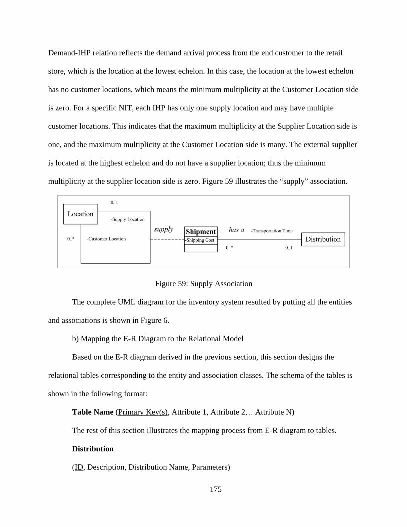
175

Demand-IHP relation reflects the demand arrival process from the end customer to the retail

store, which is the location at the lowest echelon. In this case, the location at the lowest echelon

has no customer locations, which means the minimum multiplicity at the Customer Location side

is zero. For a specific NIT, each IHP has only one supply location and may have multiple

customer locations. This indicates that the maximum multiplicity at the Supplier Location side is

one, and the maximum multiplicity at the Customer Location side is many. The external supplier

is located at the highest echelon and do not have a supplier location; thus the minimum

multiplicity at the supplier location side is zero. Figure 59 illustrates the “supply” association.

Figure 59: Supply Association

The complete UML diagram for the inventory system resulted by putting all the entities

and associations is shown in Figure 6.

b) Mapping the E-R Diagram to the Relational Model

Based on the E-R diagram derived in the previous section, this section designs the

relational tables corresponding to the entity and association classes. The schema of the tables is

shown in the following format:

Table Name (Primary Key(s), Attribute 1, Attribute 2… Attribute N)

The rest of this section illustrates the mapping process from E-R diagram to tables.

Distribution

(ID, Description, Distribution Name, Parameters)

176

The Distribution entity is mapped to Distribution Table. An ID field is added as the

primary key of the Distribution Table.

Location

(ID, Name, Echelon)

The Location entity is mapped to Location Table. An ID field is added as the primary key

of the Location Table.

Item Type

(ID, Name, Unit Cost, Lost sales Cost, Weight, Cube, LeadTimeID(references

Distribution Table), LeadTimeMean, LeadTimeVar)

The Item Type entity is mapped to Item Type Table. An ID field is added as the primary

key of the Item Type Table. Item Type Table has a buried attribute LeadTimeID that implements

Item Type – Distribution association in Figure 56. The lead time mean(LeadTimeMean) and lead

time variance(LeadTimeVar) for the lead time distribution are also stored in the Item Type table.

Demand Generator

(ItemTypeID(reference Item Type Table), LocationID(reference Location Table), Name,

TBAID(reference Distribution Table), DemandSizeID(reference Distribution Table),

AnnualDemandMean, AnnualDemandVar)

The “arrive at” association in Figure 57 is mapped to Demand Generator Table. The

association attribute, name, is turned into an attribute column in the Demand Generator Table.

The TBAID is buried into Demand Generator Table to implement the “has a TBA” association.

The DemandSizeID is buried into Demand Generator Table to implement the “has a Demand

Size” association. The mean of annual demand (AnnualDemandMean) and the variance of

annual demand (AnnualDemandVar) are also stored in the Demand Generator table.

177

SKU

(ItemTypeID(reference Item Type Table), LocationID(reference Location Table), Initial

on Hand, Backorder Cost, Ordering Cost, Holding Charge, Policy Name, ReorderPoint,

ReorderQuantity, Min, Max, ReviewPeriod, LeadTimeMean, LeadTimeVar)

The “store at” association in Figure 58 is mapped to SKU Table. The association

attributes, initial on hand, backorder cost, ordering cost, holding charge, are turned into attribute

columns in the SKU Table. The lead time mean (LeadTimeMean) and lead time variance

(LeadTimeVar) of the SKU reordering time are also stored in the SKU table.

In order to satisfy the requirements of third normal form, the Inventory Policy entity

should be mapped to an Inventory Policy table, and the primary key of Inventory Policy Table

should be buried into SKU Table. This would increase the complexity of the table structure and

the data input process. Two revisions are made to solve this problem: (1) the attributes of the

Inventory Policy entity are stored in the SKU Table, and (2) the parameters of the inventory

policy are separated into five columns. As a result, the SKU Table violates the second normal

form since some of the attributes, such as ReorderPt, ReorderQty, Min, Max, and ReviewPeriod,

are not dependent on the primary keys. These columns are determined by the non-primary key

column Policy Name. As aforementioned, the purpose of denormalizing the SKU table is to

reduce the complexity of the data structure. Compared to storing the information of Inventory

Policy in a separate table, putting it in the SKU table makes it easier to input all the SKU

information in one table.

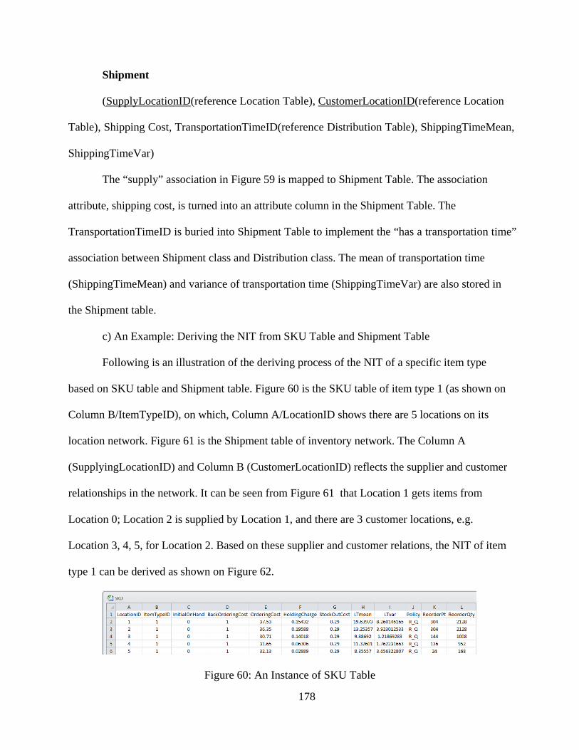
178

Shipment

(SupplyLocationID(reference Location Table), CustomerLocationID(reference Location

Table), Shipping Cost, TransportationTimeID(reference Distribution Table), ShippingTimeMean,

ShippingTimeVar)

The “supply” association in Figure 59 is mapped to Shipment Table. The association

attribute, shipping cost, is turned into an attribute column in the Shipment Table. The

TransportationTimeID is buried into Shipment Table to implement the “has a transportation time”

association between Shipment class and Distribution class. The mean of transportation time

(ShippingTimeMean) and variance of transportation time (ShippingTimeVar) are also stored in

the Shipment table.

c) An Example: Deriving the NIT from SKU Table and Shipment Table

Following is an illustration of the deriving process of the NIT of a specific item type

based on SKU table and Shipment table. Figure 60 is the SKU table of item type 1 (as shown on

Column B/ItemTypeID), on which, Column A/LocationID shows there are 5 locations on its

location network. Figure 61 is the Shipment table of inventory network. The Column A

(SupplyingLocationID) and Column B (CustomerLocationID) reflects the supplier and customer

relationships in the network. It can be seen from Figure 61 that Location 1 gets items from

Location 0; Location 2 is supplied by Location 1, and there are 3 customer locations, e.g.

Location 3, 4, 5, for Location 2. Based on these supplier and customer relations, the NIT of item

type 1 can be derived as shown on Figure 62.

Figure 60: An Instance of SKU Table

179

Figure 61: An Instance of Shipment Table

Figure 62: NIT of Item Type 1

180

Appendix 3: Data Representation in Java Classes and the Data Generation Algorithm

This appendix contains two parts. The first part illustrates the implementation of data

models (discussed in Section 4.1 and Appendix 2) using Java classes. Based on the developed

Java classes, the second part demonstrates the data generation processes (discussed in Section

4.2.2.2) using several algorithms.

Data Representation in Java Classes

Each table designed in the Data Modeling process is implemented as a Java class. The

attributes and data types of these Java classes are summarized in the data modeling appendix. In

this table, the first column is the Java Class name, the second column is the corresponding table

name, the third column is the attribute name in the tables, the fourth column is the corresponding

attributes represented in Java, and fifth column is the Java data type for the fourth column. The

data types presented in the fifth column could be the original Java data types or the data types

(classes) created in this research. Except for the foreign keys, the Java data type is selected based

on the attribute description in the table design. The data types of the foreign keys are

implemented by the data type where the foreign keys reference to. For example, in Item Type

table, the attribute LeadTimeID is used to reference Distribution Table; in the corresponding

Java class ItemTypeDM, the LeadTimeID attribute is implemented by a class attribute

myLeadTime, whose data type is CDFInfo class (since the Distribution Table is implemented as

CDFInfo class). The attribute myLocationNetwork and the data type LocationNetwork in

ItemTypeDM class will be discussed later. The domain of the data type CDFName is {Normal,

Beta, Lognormal, Gamma, Weibull, PearsonType5, PearsonType6, Triangular, Bernoulli,

Geometric, ShiftedGeometric, Poisson,VConstant, Exponential, DUniform, Uniform, JohnsonB,

LogLogistic, NegativeBinomial, Binomial, DEmpirical}.

181

Table 39: Java Classes Based on Tables

Java Class Name Table Name Attributes in Table Attributes in Java Data Type CDFInfo Distribution

ID myID int Description myDescription String Distribution Name myType CDF name Parameters myParams String

LocationDM Location ID myID int Name myName String Echelon myLevel int

ItemTypeDM Item Type ID myID int Name myName String Unit Cost myCost double Lost sales Cost myLostSaleCost double Weight myWeight double Cube myCube double LeadTimeID myLeadTime CDFInfo LeadTimeMean myLeadTimeATESmean double LeadTimeVar myLeadTimeATESvar double myLocationNetwork LocationNetw

ork SKUDM SKU LocationID myLocation LocationDM

ItemTypeID myItemType ItemTypeDM Initial on Hand myInitialOnHand int Ordering Cost myOrderingCost double Holding Charge myHoldingCharge double Stockout Cost myStockOutCost double Policy Name myPolicy String ReorderPoint myReorderPt int ReorderQuantity myReorderQty int ReviewPeriod myReviewPeriod double Min myMin int Max myMax int LeadTimeMean myLeadTimeMean double LeadTimeVar myLeadTimeVar double

ShipmentDM Shipment SupplyLocationID mySupplyingLocation LocationDM CustomerLocationID myCustomerLocation LocationDM TransportationTimeID myShippingTime CDFInfo ShippingTimeMean myShippingTimeMean double ShippingTimeVar myShippingTimeVar double Shipping Cost myShippingCost double

DemandGeneratorDM

Demand Generator

LocationID mySupplier LocationDM ItemTypeID myItemType ItemTypeDM TBAID myTimeBtwEvents CDFInfo DemandSizeID myAmt CDFInfo Name myName String AnnualDemandMean myAnnualDemandMean double AnnualDemandVar myAnnualDemandVar double

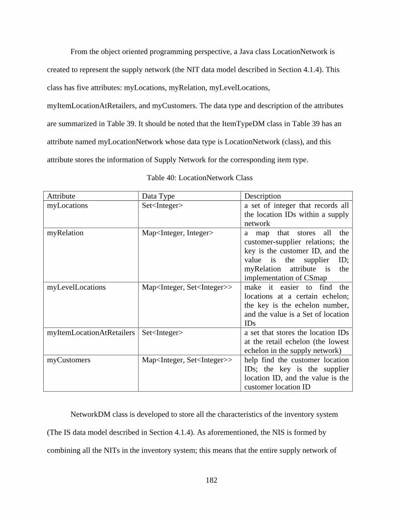
182

From the object oriented programming perspective, a Java class LocationNetwork is

created to represent the supply network (the NIT data model described in Section 4.1.4). This

class has five attributes: myLocations, myRelation, myLevelLocations,

myItemLocationAtRetailers, and myCustomers. The data type and description of the attributes

are summarized in Table 39. It should be noted that the ItemTypeDM class in Table 39 has an

attribute named myLocationNetwork whose data type is LocationNetwork (class), and this

attribute stores the information of Supply Network for the corresponding item type.

Table 40: LocationNetwork Class

Attribute Data Type Description myLocations Set<Integer> a set of integer that records all

the location IDs within a supply network

myRelation Map<Integer, Integer> a map that stores all the customer-supplier relations; the key is the customer ID, and the value is the supplier ID; myRelation attribute is the implementation of CSmap

myLevelLocations Map<Integer, Set<Integer>> make it easier to find the locations at a certain echelon; the key is the echelon number, and the value is a Set of location IDs

myItemLocationAtRetailers Set<Integer> a set that stores the location IDs at the retail echelon (the lowest echelon in the supply network)

myCustomers Map<Integer, Set<Integer>> help find the customer location IDs; the key is the supplier location ID, and the value is the customer location ID

NetworkDM class is developed to store all the characteristics of the inventory system

(The IS data model described in Section 4.1.4). As aforementioned, the NIS is formed by

combining all the NITs in the inventory system; this means that the entire supply network of

183

inventory system information can be represented by modeling the NIS. The NIS is implemented

as an attribute myLocationNetwork in the NetworkDM whose data type is LocationNetwork . As

mentioned in Section 2.1 and repeated here as a reminder, Cohen et al. (1986) point out that the

characteristics of an multi-echelon multi-item inventory system includes: 1) number of products,

(2) number of echelons, (3) network structure (series, arborescence, general), (4) periodic versus

continuous review, (5) cost/service tradeoff measures, (6) demand process class, and (7) lead

time and distribution mechanisms, etc. The attributes of NetworkDM class will store all of these

characteristics. The data type and description of the attributes are summarized in Table 41.

Table 41: NetworkDM Class

Attribute Data Type Description myCDFs Map<Integer, CDFInfo> Store the CDFInfo objects

(distributions) that are used in inventory systems; the Integer stores the ID of the CDFInfo object

myItemTypes Set<ItemTypeDM> Store the item types in the inventory systems

myLocations Map<Integer, LocationDM> Store the locations in the inventory systems

myLevelLocations Map<Integer, LocationDM> Permits easy look up of locations by echelon.

myShipments Map<LocationDM, ShipmentDM>

Store the shipping information for each customer location.

mySKUs Set<SKUDM> Store the SKUs in the inventory systems.

myDemandGeneratorDMs Set<DemandGeneratorDM> Store the DemandGeneratorDM objects in the inventory systems

myLocationNetwork LocationNetwork Store the Supply Network of the inventory systems

Data Generation Algorithms

The rest of this appendix uses several algorithms to illustrate the data generation

processes. The inputs of the data generation and four main data generation steps are summarized

184

in Section 4.2.2.2. The step 1 corresponds to Algorithm 2. Step 2, 3 and 4 correspond to the three

for loops in Algorithm 1.

Algorithm 1: The data generation procedure generate a NetworkDM object networkdm; generate an integer value NE using 𝐷𝑁𝑁; create a LocationNetwork object LN and initialize its attributes; (refer to Algorithm 2) set networkdm.myLocationNetwork= LN; create and add the LocationDM objects to networkdm.myLocations using LN ;(refer to Algorithm 4) create and add the ShipmentDM objects to networkdm.myShipments using LN (refer to Algorithm 5) for loopCounter = 1 to NI create an ItemTypeDM object itemtypedm; set itemtypedm.myID = loopCounter; set itemtypedm.myName = “Item Type loopCounter”; generate a double value dblUnitCost using 𝐷𝑈𝐼; set itemtypedm.myCost = dblUnitCost; generate a double value dblLSCR using 𝐷𝐿𝑆𝐼; set itemtypedm. myLostSaleCost= dblUnitCost* dblLSCR; generate a double value dblLeadTime using 𝐷𝐿𝐿𝑁𝑆; generate a double value dblLTVTMR Value using 𝐷𝐿𝐿𝐷; set dblLeadTimeVar = dblLeadTime * doubleLTVTMR; set itemtypedm. myLeadTimeATESmean= dblLeadTime; set itemtypedm. myLeadTimeATESvar= dblLeadTimeVar; add itemtypedm to networkdm.myItemTypes; increase loopCounter by 1; end for for each itemtypedmElement in networkdm.myItemTypes create a LocationNetwork object locationNetwork; set the attributes of locationNetwork using buildNewNIT method; (refer to Algorithm 6) for each intLocaitonID in locationNetwork.myLocations get locationdm from networkdm.myLocations using intLocaitonID; set intEchelonValue = the locationdm.myLevel; if (!intEchelonValue == 0) then create a SKUDM object skudm; set skudm.myLocation = locationdm; set skudm.myItemType = itemtypedmElement; generate a double value dblHoldingCharge by 𝐷𝐻𝐼;

185

set skudm.myHoldingCharge = dblHoldingCharge; generate a double value dblOrderingCost by 𝐷𝑂𝐼; set skudm.myOrderingCost = dblOrderingCost; set skudm. myStockOutCost= itemtypedmElement.myLostSaleCost; generate a double value dblLTMean using 𝐷𝐿𝐿𝐼𝐻𝐿; set skudm. myLeadTimeMean= dblLTMean; generate a double value dblLTVTMR Value using 𝐷𝐿𝐿𝐷; set dblLTV= dblLTMean * dblLTVTMR; set skudm. myLeadTimeVar= dblLTV; add skudm to networkdm.mySKUs; end if end for each set itemtypedmElement.myLocationNetwork = locationNetwork; end for each for each skudmElement in networkdm.mySKUs set locationdm = skudmElement.myLocation; set intEchelonValue = locationdm.myLevel; if (intEchelonValue == NE) set skudmElement.myPolicy =” R_Q”; set skudmElement.myReorderPt = 1; set skudmElement.myReorderQty = 1; set intLocationID = locationdm.myID ; set itemtypedm =skudmElement.myItemType; set intItemTypeID = itemtypedm.myID; generate a double value dblDM using 𝐷𝐷𝑅; generate a double value dblDVTMR using 𝐷𝐷𝐷; set dblDV= dblDM * dblDVTMR; create a DemandGeneratorDM object dgdm; set dgdm.myName = “DG for Item Type intItemTypeID Location intLocationID” ; set dgdm.mySupplier = locationdm; set dgdm.myItemType = itemtypedm; set dgdm. myAnnualDemandMean = dblDM; set dgdm. myAnnualDemandVar = dblDV; add dgdm to networkdm.myDemandGeneratorDMs; end if end for each Algorithm 2: generateNetwork() in LocationNetwork class addLocation(0, 0) ;(refer to Algorithm 3) set intCumulativeNum = 0; set intCurrentLevel = 1; define Set<Integer> locationSet;

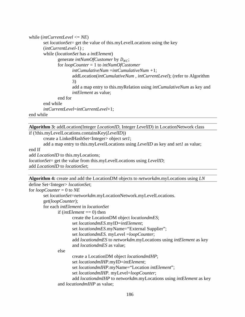
186

while (intCurrentLevel <= NE) set locationSet= get the value of this.myLevelLocations using the key (intCurrentLevel-1) ; while (locationSet has a intElement) generate intNumOfCustomer by 𝐷𝑁𝐼; for loopCounter = 1 to intNumOfCustomer intCumulativeNum =intCumulativeNum +1; addLocation(intCumulativeNum , intCurrentLevel); (refer to Algorithm 3) add a map entry to this.myRelation using intCumulativeNum as key and intElement as value; end for end while intCurrentLevel=intCurrentLevel+1; end while Algorithm 3: addLocation(Integer LocationID, Integer LevelID) in LocationNetwork class if (!this.myLevelLocations.containsKey(LevelID)) create a LinkedHashSet<Integer> object set1; add a map entry to this.myLevelLocations using LevelID as key and set1 as value; end If add LocationID to this.myLocations; locationSet= get the value from this.myLevelLocations using LevelID; add LocationID to locationSet; Algorithm 4: create and add the LocationDM objects to networkdm.myLocations using LN define Set<Integer> locationSet; for loopCounter = 0 to NE set locationSet=networkdm.myLocationNetwork.myLevelLocations. get(loopCounter); for each intElement in locationSet if (intElement == 0) then create the LocationDM object locationdmES; set locationdmES.myID=intElement; set locationdmES.myName=“External Supplier”; set locationdmES. myLevel =loopCounter; add locationdmES to networkdm.myLocations using intElement as key and locationdmES as value; else create a LocationDM object locationdmIHP; set locationdmIHP.myID=intElement; set locationdmIHP.myName=“Location intElement”; set locationdmIHP. myLevel=loopCounter; add locationdmIHP to networkdm.myLocations using intElement as key and locationdmIHP as value;

187

end if end for each increase loopCounter by 1; end for Algorithm 5: create and add the ShipmentDM objects to networkdm.myShipments using LN for each mapEntry in networkdm. myRelation.entrySet() set intCustomerID = the key of the mapEntry; set intSupplierID = the value of the mapEntry; generate a double value dblShippingTime using 𝐷𝐿𝐿𝐼𝐻𝐿; generate a double value dblLTVTMR value using 𝐷𝐿𝐿𝐷; set dblLTV= dblShippingTime * dblLTVTMR; create a ShipmentDM object shipmentdm; set shipmentdm.mySupplyingLocation.myID= intSupplierID; set shipmentdm.myCustomerLocation.myID= intCustomerID; set shipmentdm.myShippingTimeMean= dblShippingTime; set shipmentdm.myShippingTimeVar= dblLTV; end for each Algorithm 6: buildNewNIT method in LocationNetwork class For each itemtypedmElement in networkdm.myItemTypes create a new LocationNetwork object locationNetwork; set locationNetwork =networkdm.myLocationNetwork; set intLocationIDSet=get the value of locationNetwork.myLevelLocations using the key NE; for each intElement in intLocationIDSet generate a double value dblProb~Uniform(0,1); if (dblProb <= 𝐶𝐼) then add intElement to locationNetwork.myItemLocationAtRetailers; end if end for each for loopCounter= NE to 1 set intLevelLocationsSet = get the value of locationNetwork. myLevelLocations using the key loopCounter; if (loopCounter == NE) for each intElement in intLevelLocationsSet if (locationNetwork. myItemLocationAtRetailers does not contain the element intElement ) delete the element intElement from locationNetwork. myLocations; delete the element intElement from intLevelLocationsSet; delete the entry from locationNetwork.myRelation using the key intElement; end if

188

end for each else for each intElement in intLevelLocationsSet set intCustomerIDSet=get the value of locationNetwork.myLevelLocations using the key (loopCounter+1); set existCustomer=False; for each intElement2 in intCustomerIDSet if ( exist an entry using intElement2 as the key and intElement as value in locationNetwork.myRelation) set existCustomer=True; end if end for each if (existCustomer=False) delete the element intElement from locationNetwork.myLocations; delete the element intElement from intLevelLocationsSet; delete the entry from locationNetwork.myRelation using the key intElement; end if end for each end if decrease loopCounter by 1; end for end for each

189

Appendix 4: Data Analysis for Inputs

This appendix shows the details about the data analysis processes. The purpose of data

analysis is to generate data that represents real world inventory system. The data analysis serves

two main goals: 1) determine the data range for the attributes, and 2) investigate the relationships

between attributes.

The attributes studied in this appendix are as follows:

𝐼 ≡ unit cost of an item

𝑏 ≡ lost sales cost of an item

𝜆 ≡ demand rate at retail store

𝜎𝑅 ≡ standard deviation of demand at retail store R

𝐴 ≡ ordering cost

𝐼 ≡ inventory holding charge

𝐸(𝐶𝐺𝑁𝑆) ≡ mean lead time at external supplier

𝐸(𝐶𝐺𝐼𝐻𝐿) ≡ mean lead time at an inventory holding point

𝑉𝑙𝑟(𝐶𝐺𝑁𝑆) ≡ variance of lead time at external supplier

𝑉𝑙𝑟(𝐶𝐺𝐼𝐻𝐿) ≡ variance of lead time at an inventory holding point

Exhibit 33: Attributes List for the Study

The rest of this appendix discusses the quantification of these attributes.

The Range of Input Values

The inventory holding charge is calculated by dividing the inventory holding cost using

the number of on hand inventory. The inventory holding charge consists of capital costs,

inventory service costs, storage space costs, and inventory risk cost (REM Associates). REM

Associates collect the estimate of carrying costs as a percentage of inventory value from 13

190

textbooks. According to the values from these textbook, the range of the inventory holding

charge is from 12%-35%.

The ordering cost is the expense spent on placing an order. This cost includes the

activities related to ordering process, such as making invoices, billing, arranging shipping, etc.

P&G estimated that the cost of each invoicing is between $35 to $75 (Lee et al. 1997). In this

dissertation, the shipping cost is also included as part of the ordering cost. In the scenario

discussed in Section 1, the inventory system considered is an international business that sourcing

the products from different countries; thus, the cost of international shipping should be

considered. Considering shipping a 40 foot container from China to the US as an example, a total

of $7,000 shipping cost may occur with the $4000 for ocean freight and $3000 for inland

trucking. It should be noted that this international shipping cost only occurs from external

supplier to the warehouses located at echelon 1. Thus, the ordering cost range for inventory

holding points (IHPs) located at 1st echelon and other echelons should be different. Based on

above observations, in this dissertation the range of ordering cost is determined as [3,000, 10,000]

for IHPs located at 1st echelon, and [100, 3000] for other IHPs. It’s assumed here that each order

triggers a shipment, and the consolidation of different items in one shipment is not considered.

The research conducted by Deshpande et al. (2003) provides some insights about

attribute values, such as unit cost, demand rate and lead time. The authors investigate the data

from the U.S. military weapon system. They select a representative 21 weapon system containing

200,000 service parts and conduct a series of data analysis. Table 42 and Table 43 summarize

some statistics that directly related to this dissertation. This inventory system has characteristics

of low demand, high item cost and long production lead time. In Table 42, the production lead

time is related to the lead time at external supplier. Also, the LRT in Table 43 corresponds to the

191

lead time at an inventory holding point. LRT is the abbreviation for Logistics Response Time

which means the lead time needed to fulfill a customer order.

Table 42: Part Attributes for Weapon System

Mean Std Production Lead Time ($) 173 102 Demand Frequency (yearly) 16 86 Unit Price ($) 242.5 314

Table 43: Average Response Time (LRT) by Cost Categories

Unit Price Very Low(VL) Low (L) Medium (M) High (H) Very High (VH) ($) [$0,$150] [$150,$500] [$500,$1000] [$10,000,$200,000] [$200,000+]

Average LRT (days) 26.3 29 33.7 54.8 97.4 No. of Parts 19.80% 14.70% 40.80% 22.70% 2%

The inventory system described in Section 1 has some differences with the system

studied in Deshpande et al. (2003). The products sold in the inventory system described in

Section 1 are categorized as Consumer Packaged Goods (CPG) which has characteristics of high

demand, low cost and short production lead time. In order to get some insights in the CPG, data

from Tmall.com was collected, the largest B2C (business-to-consumer) online retail platform in

Asia.

The data collection from Tmall.com serves the following two purposes: 1) investigate the

values range for unit cost, annual demand and shipping cost; and 2) investigate the direct or

inverse proportional relationship between unit cost, annual demand and shipping cost. Sixty

observations that covering 15 major categories and 60 sub-categories were collected. Each

observation is the top seller in that sub-category. Data for three attributes are collected: 1) the

unit price in Chinese Yuan (CNY), 2) monthly demand in units, and 3) shipping cost in CNY.

192

The collected data is shown in Table 44. It should be noted that: 1) the estimated annual sales for

each item is calculated by the monthly sales times twelve, and 2) in the shipping cost column, the

asterisk before some values means that the shipping cost is not available for that category, and

the values are found from similar items.

193

Table 44: Data from Tmall

Category Sub-Category Price

(CNY) Estimated Annual Sales Shipping Cost (CNY) 1 Appliances Air Conditioners 3499 17,580 *180

Humidifiers 89 486,648 20 Laundry 1299 21,924 *380 Microwave Ovens 699 22,392 300 Refrigerators 1399 46,596 *100 Vacuums 2035 101,148 200

2 Automotive Interior Accessories 26 139,932 20 Tools & Equipment 248 90,312 500 Wheels & Tires 460 2,628 500

3 Baby Baby Food 182.4 80,748 37 Baby Toys 1.5 1,884,336 15

4 Beaty Bath 129 214,536 30 fragrance 19.9 129,840 20 Hair Care 68 209,724 15 Makeup 9.98 337,140 5 skin care 9.9 986,352 8

5 Books Biographies 46.8 49,452 30 Children's Books 69 118,500 15 Education & Reference 36.8 134,472 15

6 clothing men's clothing 19.8 947,268 20 women's clothing 23.98 1,304,376 30 underwear 6.5 1,193,004 20 accessories 1.68 2,292,780 18

7 Electronics Camera 559 27,552 50 Cell Phone 75 166,368 15 Desktops 3940 2,700 300 Kitchen 65 167,328 20 Laptops 5146.5 13,944 50 Office Electronics 58 66,456 20

8 Health &

Personal Care

House Supplies 4.9 276,000 *15 Personal Care 29.9 1,079,424 *20 Medical Supplies 299 120,360 *20 Nutrition 11 625,596 *15

9 Home Bedding 889 106,680 20 Cleaning Supplies 65 323,028 20 Decorating 226 33,660 20 Furniture 1698 14,772 *320 Storage 329 31,296 *120

10 Jewelry Bracelets 46.8 93,984 20 Earrings 218 7,788 35 Necklaces 179 59,628 20 Rings 65 37,944 20 watch 399 254,940 20

11 Luggage &

Bag

Backpacks 320 66,012 30 Briefcases 198 293,520 20 Luggage 239 311,652 50 wallet 69 236,352 20

12 Office Products office furniture 299 38,016 *175 office supplies 4.7 90,540 15

13 shoe men's shoe 98.82 212,232 60 women's shoe 138 108,792 20

14 Software Accounting 480 2,316 *20 Business & Office 328 2,688 *20 Education & Reference 13 368,196 *15

15 Sports &

Outdoors

Bikes 1399 16,668 *100 Water Sports 59 642,864 22 Fitness 228.58 39,816 150 Golf 29 26,436 15 Fishing 129.92 24,876 60 Clothing 59 93,924 20

194

A summary of the major statistics for Tmall data is listed in Table 45. The unit price and

the shipping cost are converted from CNY to USD (US dollar) based on the exchange rate of

6.2:1.

Table 45: The Main Statistics for Tmall Data

Min 20th percentile

80th percentile Max Mean Std

Unit Price ($) 0.24 3.87 74.19 830.08 77.35 157.51 Annual Demand 2,316 24,876 323,028 2,292,780 281,600 457,710 Shipping Cost($) 0.81 2.42 16.13 80.65 11.91 18.69

Even though the research conducted by Deshpande et al. (2003) and the data collected

from Tmall.com provide the insights into the mean demand values, the variance of an item

demand is not available. The study of demand variance can be found in Lee et al. (1997) and

Metters (1997). Lee et al. (1997) investigate the product data from two specific corporate

examples and conclude that the ranges of demand variance-to-mean ratio are [0.23, 4.7] and

[0.49, 3.37] respectively. Based on this observation, Metters (1997) conducts an experimental

design to test the bullwhip effect using the variance-to-mean ratios as 0.5, 2 and 4. Based on the

information from aforementioned two articles, in this dissertation, the range of demand variance-

to-mean ratio is considered as [0.1, 4].

The lost-sale penalty cost occurs when the demand is unsatisfied. In the experimental

design conducted by Metters (1997), the lost-sale penalty cost is set to be 0, 50% or 100% of the

production cost. Based on these values, the range of the lost-sale-cost-to-unit-cost ratio is set to

be [0.1,1] in this dissertation.

Ehrhardt (1984) and Chaharsooghi and Heydari (2010) study the impact of lead time on

SC performances. Both of these two studies investigate the effects of variance of lead time on the

supply chain performance such as inventory holding cost. In the experiments, Ehrhardt (1984)

195

vary the lead time variance-to-mean ratio from 0 to 100%, and Chaharsooghi and Heydari (2010)

select the lead time variance-to-mean ratio from 1.7% to 200%. Based on these two studies, the

range of lead time variance-to-mean ratio is selected as [0.01, 2] in this dissertation.

Based on the aforementioned studies, the range of input values are summarized in Table

7.

The Relationship between Attributes

The purpose in this part is to test the relationships between three attributes (unit price,

mean annual demand and shipping cost) collected from Tmall (Table 44), especially to test the

1st and 3rd assumptions mentioned in Exhibit 23. The simple linear regression considering a

single repressor x and response variable Y is used to analyze the two assumptions.

Assumption 1: Average annual demand of an item is inversely proportional to its unit

cost.

Selecting the Price as x and the Estimated Annual Sales as Y, the regression analysis from

Minitab is shown in Exhibit 34. From the ANOVA table, it can be seen that the regression model

is significant at p=0.05. The regression coefficient is -119, which means that the annual demand

is inversely proportional to price.

Regression Analysis: Annual Demand versus Price The regression equation is Annual Demand = 338856 - 119 Price Predictor Coef SE Coef T P Constant 338856 64311 5.27 0.000 Price -119.39 59.51 -2.01 0.050 S = 446412 R-Sq = 6.5% R-Sq(adj) = 4.9% Analysis of Variance

196

Source DF SS MS F P Regression 1 8.02006E+11 8.02006E+11 4.02 0.050 Residual Error 58 1.15584E+13 1.99283E+11 Total 59 1.23604E+13

Exhibit 34: Regression Analysis: Annual Demand versus Price

Assumption 3: The ordering cost is directly proportional to its unit cost.

Selecting the Price as x and the Shipping cost as Y, the regression analysis from Minitab

is shown in Exhibit 35. From the ANOVA table, it can be noted that the regression is significant

at p=0.003. The regression coefficient is 0.0448, which means that the shipping cost is directly

proportional to price.

Regression Analysis: Shipping Cost versus Price The regression equation is Shipping Cost = 52.3 + 0.0448 Price Predictor Coef SE Coef T P Constant 52.33 15.59 3.36 0.001 Price 0.04484 0.01443 3.11 0.003 S = 108.226 R-Sq = 14.3% R-Sq(adj) = 12.8% Analysis of Variance Source DF SS MS F P Regression 1 113136 113136 9.66 0.003 Residual Error 58 679348 11713 Total 59 792484

Exhibit 35: Regression Analysis: Shipping Cost Versus Price

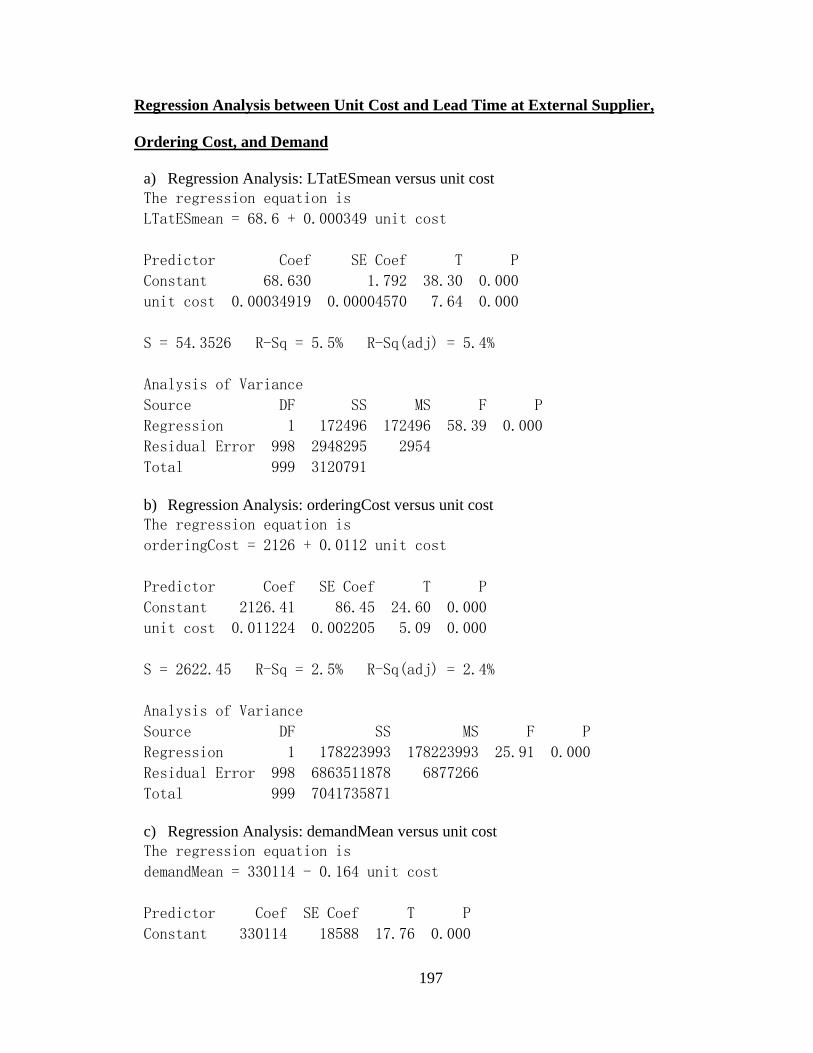
197

Regression Analysis between Unit Cost and Lead Time at External Supplier,

Ordering Cost, and Demand

a) Regression Analysis: LTatESmean versus unit cost The regression equation is

LTatESmean = 68.6 + 0.000349 unit cost

Predictor Coef SE Coef T P

Constant 68.630 1.792 38.30 0.000

unit cost 0.00034919 0.00004570 7.64 0.000

S = 54.3526 R-Sq = 5.5% R-Sq(adj) = 5.4%

Analysis of Variance

Source DF SS MS F P

Regression 1 172496 172496 58.39 0.000

Residual Error 998 2948295 2954

Total 999 3120791

b) Regression Analysis: orderingCost versus unit cost The regression equation is

orderingCost = 2126 + 0.0112 unit cost

Predictor Coef SE Coef T P

Constant 2126.41 86.45 24.60 0.000

unit cost 0.011224 0.002205 5.09 0.000

S = 2622.45 R-Sq = 2.5% R-Sq(adj) = 2.4%

Analysis of Variance

Source DF SS MS F P

Regression 1 178223993 178223993 25.91 0.000

Residual Error 998 6863511878 6877266

Total 999 7041735871 c) Regression Analysis: demandMean versus unit cost The regression equation is

demandMean = 330114 - 0.164 unit cost

Predictor Coef SE Coef T P

Constant 330114 18588 17.76 0.000

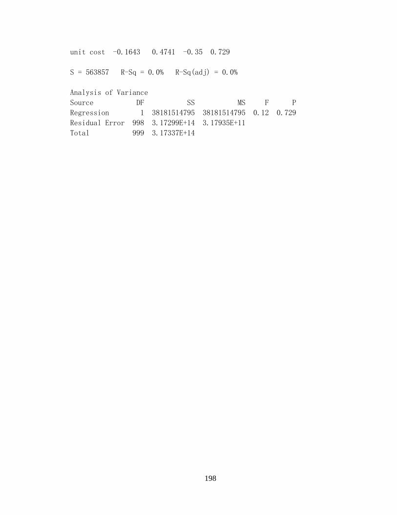
198

unit cost -0.1643 0.4741 -0.35 0.729

S = 563857 R-Sq = 0.0% R-Sq(adj) = 0.0%

Analysis of Variance

Source DF SS MS F P

Regression 1 38181514795 38181514795 0.12 0.729

Residual Error 998 3.17299E+14 3.17935E+11

Total 999 3.17337E+14

199

Appendix 5: The Experimental Data for ABC Classification

This appendix illustrates the organization of the experimental results and the calculation

of the across scenario means. The experimental data for ABC Classification is introduced as an

example in this appendix, and the experimental results for NIT classification and K-Means

clustering follow the same organization. After implementing the ABC classification, the

performances of the ABC classification are listed in Table 46. The levels for the experiment

parameters (factor A to L are introduced in Table 21) are recorded in the columns from A to L.

The low level is represented using “-1” and the high level is represented as “1”. In addition, the

column “NG” records the levels for number of groups and the column “S1” records the levels for

classification criteria. The last three columns record the performance measures, i.e., percent

increase of clustering penalty cost (%CPC), SSE and grouping time (GT).

A total of 1024 scenarios are used to compare the classification criteria NIC and NADU.

Table 46: The Performance of ABC Classification

No. A B C D E F G H J K L NG S1 %CPC SSE GT 1 -1 -1 -1 -1 -1 -1 -1 -1 -1 -1 -1 -1 -1 19.5 1.26E+09 0.169 2 -1 -1 -1 -1 -1 -1 -1 1 -1 -1 1 -1 -1 16.6 2.44E+09 0.089 3 -1 -1 -1 -1 1 1 -1 -1 -1 1 1 -1 -1 15.2 2.24E+10 0.228 4 -1 1 1 1 1 1 -1 -1 1 1 1 -1 -1 16.2 2.90E+10 0.132 5 -1 1 1 1 1 1 -1 1 -1 -1 -1 -1 -1 19.2 6.83E+09 0.033

… … -1 -1 -1 -1 -1 -1 -1 -1 -1 -1 -1 -1 17.5 1.23E+09 0.024 1023 -1 1 1 1 1 1 1 1 1 1 1 -1 -1 15.7 2.91E+10 0.123 1024 1 -1 -1 -1 -1 -1 -1 -1 -1 -1 1 -1 -1 15.5 2.39E+09 0.042

The across scenario mean for a response variable is the average of the values of all

scenarios. For example, the across scenario mean for grouping time is shown as following:

𝐺𝐺𝑚𝑐𝑟𝑡𝑎𝑎−𝑎𝑐𝑒𝑛𝑚𝑟𝑖𝑡 = � 𝐺𝐺𝑖

1024

𝑖=1

The across scenario mean for %CPC and SSE follow the same formulation.