Group Sequential Methods

for Clinical Trials

Christopher Jennison,

Dept of Mathematical Sciences,

University of Bath, UK

http://www.bath.ac.uk/�mascj

PSI, London,

22 October 2003

1

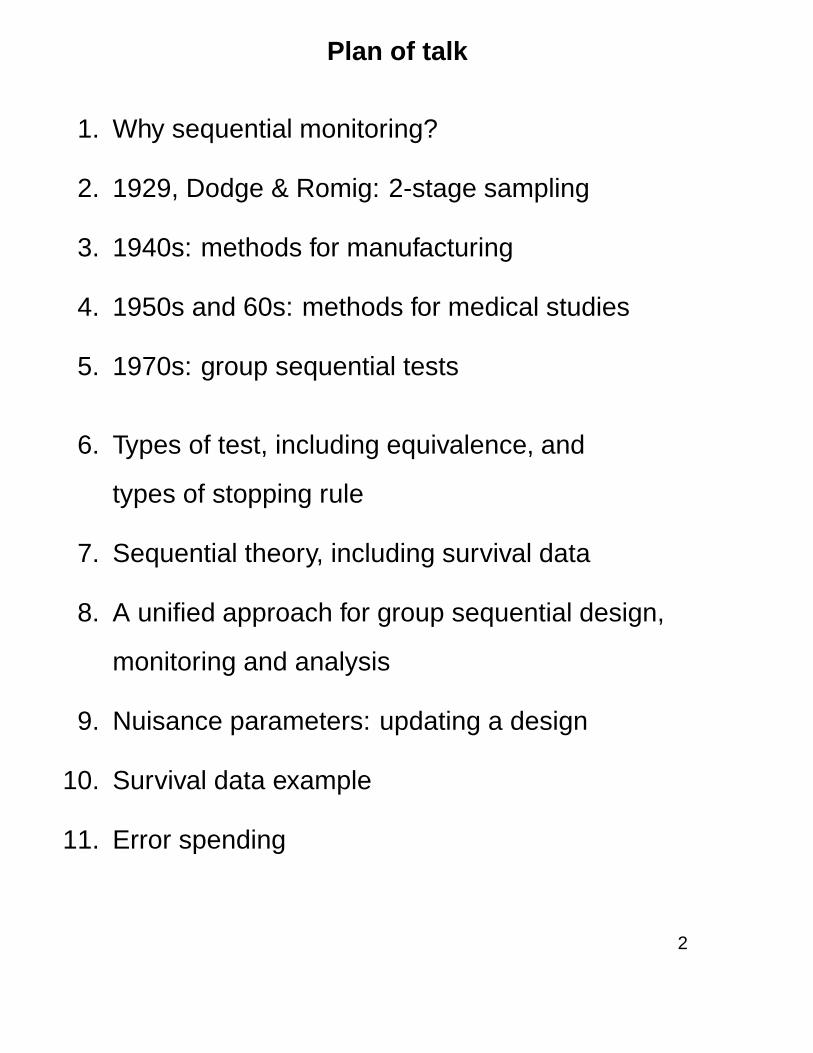
Plan of talk

1. Why sequential monitoring?

2. 1929, Dodge & Romig: 2-stage sampling

3. 1940s: methods for manufacturing

4. 1950s and 60s: methods for medical studies

5. 1970s: group sequential tests

6. Types of test, including equivalence, and

types of stopping rule

7. Sequential theory, including survival data

8. A unified approach for group sequential design,

monitoring and analysis

9. Nuisance parameters: updating a design

10. Survival data example

11. Error spending

2

1. Motivation of interim monitoring

In clinical trials, animal trials and epidemiological studies

there are reasons of

ethics

administration (accrual, compliance, . . . )

economics

to monitor progress and accumulating data.

Subjects should not be exposed to unsafe, ineffective or

inferior treatments. National and international guidelines

call for interim analyses to be performed — and reported.

It is now standard practice for medical studies to have a

Data and Safety Monitoring Board to oversee the study

and consider the option of early termination.

3

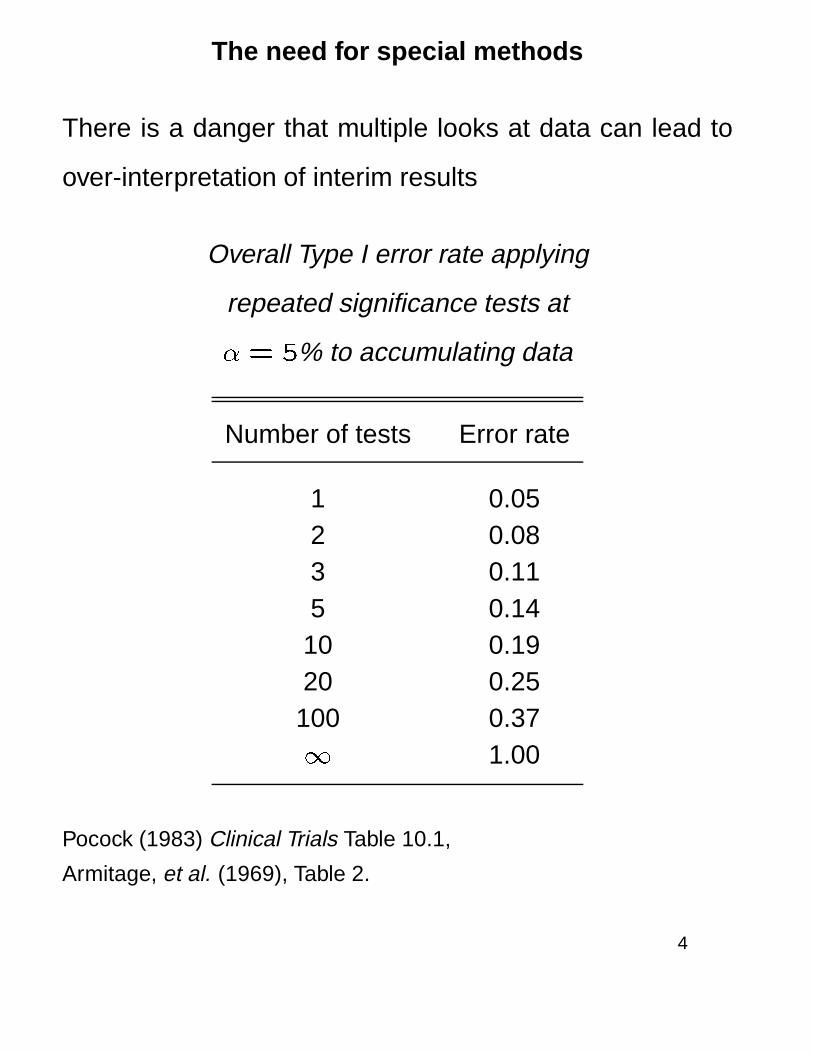
The need for special methods

There is a danger that multiple looks at data can lead to

over-interpretation of interim results

Overall Type I error rate applying

repeated significance tests at

�= 5% to accumulating data

Number of tests Error rate

1 0.052 0.083 0.115 0.14

10 0.1920 0.25

100 0.371 1.00

Pocock (1983) Clinical Trials Table 10.1,

Armitage, et al. (1969), Table 2.

4

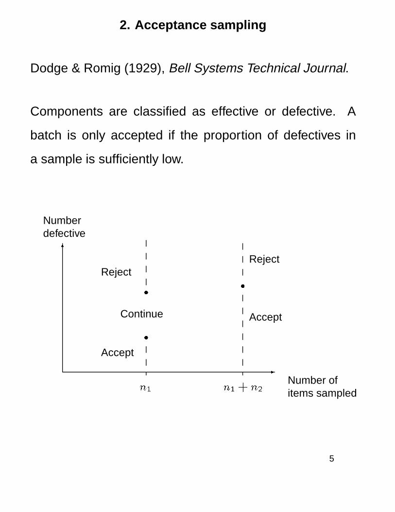
2. Acceptance sampling

Dodge & Romig (1929), Bell Systems Technical Journal.

Components are classified as effective or defective. A

batch is only accepted if the proportion of defectives in

a sample is sufficiently low.

-

Number ofitems sampled

n1 n1+ n2

6

Numberdefective

Reject

�

Continue

�

Accept

Reject

�

Accept

5

3. Manufacturing production

Barnard and Wald developed methods for industrial

production and development.

Wald (1947) published his Sequential Probability Ratio

Test (SPRT) for testing between two simple hypotheses.

Stopping boundaries and continuation region

-

n

6

Sample sum

Sn

@��X�

��X���

6

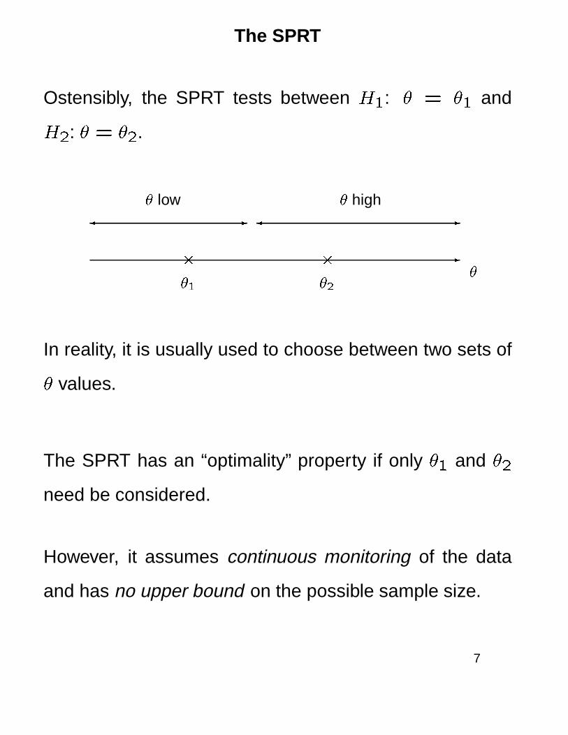
The SPRT

Ostensibly, the SPRT tests between H1: � = �1 and

H2: � = �2.

-

��

�1

�

�2

-�

� low-�

� high

In reality, it is usually used to choose between two sets of

� values.

The SPRT has an “optimality” property if only �1 and �2

need be considered.

However, it assumes continuous monitoring of the data

and has no upper bound on the possible sample size.

7

4. Sequential monitoring of clinical trials

In the 1950s, Armitage and Bross took sequential testing

from industrial applications to comparative clinical trials.

Their plans were fully sequential but with a bounded

maximum sample size.

The “restricted” test, Armitage (1957),

-

n

6

Sn

((((((((

((((((((

((((((((

((((((

hhhhhhhhhhhhhhhhhhhhhhhhhhhhhh

Accept H0

Reject H0

Reject H0

testing H0: � = 0 against � 6= 0, where � is the treatment

difference.

8

Armitage’s repeated significance test

Armitage, McPherson & Rowe (1969) applied a

significance test of H0: � = 0 after each new pair of

observations.

Numerical calculations gave the “nominal” significance

level �0 to use in each of N repeated significance tests

for an overall type I error probability �.

-

n

6

Sn

���,���

!!��

�����

��

((((((

((((

AA@lQHHaaPPPPXXXXX```````hhhhhhhhhh

Accept H0

Reject H0

Reject H0

9

5. Group sequential tests

In practice, one can only analyse a clinical trial on a small

number of occasions.

Shaw (1966): talked of a “block sequential” analysis.

Elfring & Schultz (1973): gave “group sequential” designs

to compare two binary responses.

McPherson (1974): use of repeated significance tests at a

small number of analyses.

Pocock (1977): provided clear guidelines for group

sequential tests with given type I error and power.

O’Brien & Fleming (1979): an alternative to Pocock’s

repeated significance tests.

10

Pocock’s repeated significance test

To test H0: � = 0 against � 6= 0.

Use standardised test statistics Zk, k = 1; : : : ;K.

Stop to reject H0 at analysis k if

jZkj > c:

If H0 has not been rejected by analysis K, stop and

accept H0.

-

k

6Zk

� � � �

� � � �

Reject H0

Reject H0

Accept H0

11

6. Types of hypothesis testing problems

Two-sided test:

testing H0: � = 0 against � 6= 0.

One-sided test:

testing H0: � � 0 against � > 0.

Equivalence tests:

one-sided — to show treatment A is as

good as treatment B, within a margin Æ.

two-sided — to show two treatment

formulations are equal within an

accepted tolerance.

12

A two-sided equivalence test

Conduct a test of H0: � = 0 vs � 6= 0 with type I error

rate � and power 1� � at � = �Æ.

Declare equivalence if H0 is accepted.

-

��Æ 0 Æ

6

1��

�. . .

...

.

.... . . . .

...

.

... . . .

....

.

.... . . .

...

.

....

PrfDeclare

equivalenceg

Here, � represents the “consumer’s risk.”

In design and implementation, give priority to attaining

power 1� � at � = �Æ.

13

Types of early stopping

1. Stopping to reject H0: no treatment difference

� Allows progress from a positive outcome

� Avoids exposing further patients to the inferior

treatment

� Appropriate if no further checks are needed on, say,

treatment safety or long-term effects.

2. Stopping to accept H0: no treatment difference

� Stopping “ for futility” or “abandoning a lost cause”

� Saves time and effort when a study is unlikely to lead

to a positive conclusion.

14

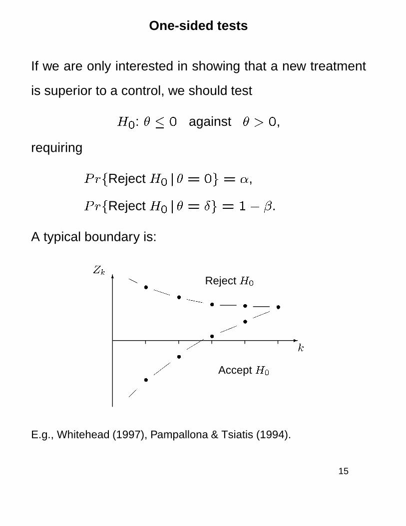
One-sided tests

If we are only interested in showing that a new treatment

is superior to a control, we should test

H0: � � 0 against � > 0,

requiring

PrfReject H0 j � = 0g = �,

PrfReject H0 j � = Æg = 1� �.

A typical boundary is:

-

k

6Zk

��

� � �

�

�

�

�

HH

PPP``̀

��

���

"""

!!!

!!!

Reject H0

Accept H0

E.g., Whitehead (1997), Pampallona & Tsiatis (1994).

15

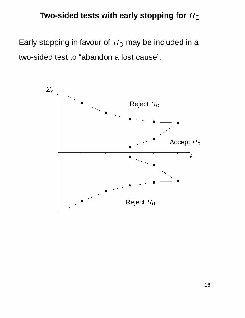
Two-sided tests with early stopping for H0

Early stopping in favour of H0 may be included in a

two-sided test to “abandon a lost cause”.

-

k

6Zk

�

��

� �

�

�

�

��

� �

�

�

HH

aaaXXX

hhh

���

���

��

!!!

���(((

PPP

QQQ

��

!!!

���(((

PPP

QQQ

Reject H0

Reject H0

Accept H0

16

One-sided tests of H0: � = 0 vs � > 0

Early stopping to

reject H0 or

accept H0

-

Ik

6Zk

�� � �

�

�

�

Reject H0

Accept H0

Early stopping only

to reject H0

-

Ik

6Zk

�� � �

Reject H0

Accept H0

Abandoning a lost

cause:

Early stopping only

to accept H0

-

Ik

6Zk

�

�

�

�

Reject H0

Accept H0

17

Two-sided tests of H0: � = 0 vs � 6= 0

Early stopping to

reject H0

-

Ik

6Zk

�� � �

�� � �

Reject H0

Reject H0

Accept H0

An inner wedge:

Early stopping to

reject H0 or

accept H0

-

Ik

6Zk

�� � �

��

�� � �

��

Reject H0

Reject H0

Accept H0

Abandoning a lost

cause:

Only an inner wedge

-

Ik

6Zk

�

��

�

��

Reject H0

Reject H0

Accept H0

18

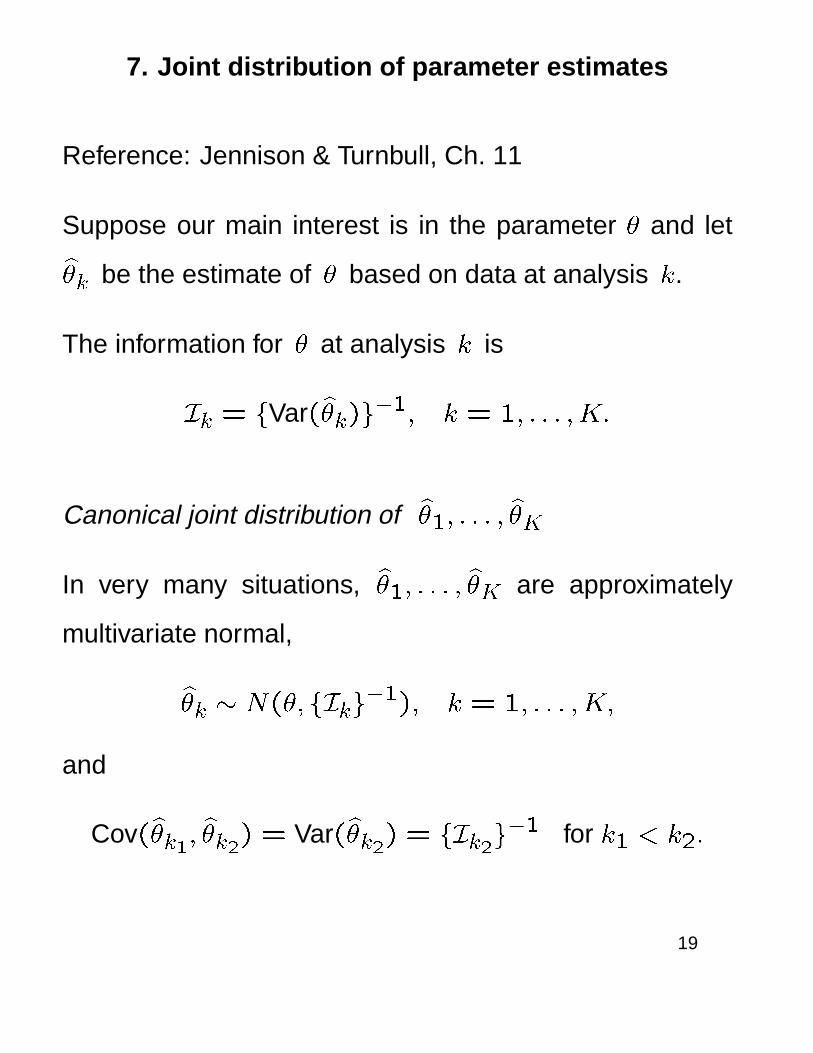
7. Joint distribution of parameter estimates

Reference: Jennison & Turnbull, Ch. 11

Suppose our main interest is in the parameter � and let

b�k be the estimate of � based on data at analysis k.

The information for � at analysis k is

Ik = fVar(b�k)g�1; k = 1; : : : ;K:

Canonical joint distribution of b�1; : : : ; b�KIn very many situations, b�1; : : : ; b�K are approximately

multivariate normal,

b�k � N(�; fIkg�1); k = 1; : : : ;K;

and

Cov(b�k1; b�k2) = Var(b�k2) = fIk2g�1 for k1 < k2:

19

Sequential distribution theory

The preceding results for the joint distribution of

b�1; : : : ; b�K can be demonstrated directly for:

� a single normal mean,

� = �A � �B; the effect size in a comparison of two

normal means.

The results also apply when � is a parameter in:

a general normal linear,

a general model fitted by maximum likelihood (large

sample theory).

So, we have the theory to support general comparisons,

including adjustment for covariates if required.

20

Canonical joint distribution of z-statistics

In testing H0: � = 0, the standardised statistic at analysis

k is

Zk =b�kq

Var(b�k) = b�kpIk:

For this,

(Z1; : : : ; ZK) is multivariate normal,

Zk � N(�pIk;1); k = 1; : : : ; K,

Cov(Zk1; Zk2) =qIk1=Ik2 for k1 < k2.

21

Canonical joint distribution of score statistics

The score statistics Sk = ZkpIk, are also multivariate

normal with

Sk � N(� Ik; Ik); k = 1; : : : ;K:

The score statistics possess the “independent increments”

property,

Cov(Sk � Sk�1; Sk0 � Sk0�1) = 0 for k 6= k0:

It can be helpful to know the score statistics behave as

Brownian motion with drift � observed at times I1; : : : ;IK .

22

Survival data

The canonical joint distributions also arise for

a) the estimates of a parameter in Cox’s proportional

hazards regression model

b) a sequence of log-rank statistics (score statistics)

for comparing two survival curves

— and to z-statistics formed from these.

For survival data, observed information is roughly

proportional to the number of failures seen.

Special types of group sequential test are needed to

handle unpredictable and unevenly spaced information

levels: see error spending tests.

23

8. Group sequential design, monitoring and analysis

To have the usual features of a fixed sample study,

� Randomisation, stratification, etc.,

� Adjustment for baseline covariates,

� Appropriate testing formulation,

� Inference on termination,

plus the opportunity for early stopping.

Response distributions:

� Normal, unknown variance

� Binomial

� Cox model or log-rank test for survival data

� Normal linear models

� Generalized linear models

24

General approach

Think through a fixed sample version of the study.

Decide on the type of early stopping, number of analyses,

and choice of stopping boundary: these will imply

increasing the fixed sample size by a certain “inflation

factor”.

In interim monitoring, compute the standardised statistic

Zk at each analysis and compare with critical values

(calculated specifically in the case of an error spending

test).

On termination, one can obtain P-values and confidence

intervals possessing the usual frequentist interpretations.

25

Example of a two treatment comparison,

normal response, 2-sided test

Cholesterol reduction trial

Treatment A: new, experimental treatment

Treatment B: current treatment

Primary endpoint: reduction in serum cholesterol level

over a four week period

Aim: To test for a treatment difference.

High power should be attained if the mean cholesterol

reduction differs between treatments by 0.4 mmol/l.

DESIGN — MONITORING — ANALYSIS

26

DESIGN

How would we design a fixed-sample study?

Denote responses by

XAi, i= 1; : : : ; nA , on treatment A,

XBi, i = 1; : : : ; nB , on treatment B.

Suppose each

XAi � N(�A; �2) and XBi � N(�B; �

2):

Problem: to test H0: �A = �B with

two-sided type I error probability � = 0:05

and power 0.9 at j�A � �Bj = Æ = 0:4.

We suppose �2 is known to be 0.5.

(Facey, Controlled Clinical Trials, 1992)

27

Fixed sample design

Standardised test statistic

Z =�XA � �XBq

�2=nA+ �2=nB

:

Under H0, Z � N(0;1) so reject H0 if

jZj > ��1(1� �=2):

Let �A � �B = �. If nA = nB = n,

Z � N(�q

2�2=n;1)

so, to attain desired power at � = Æ, aim for

n = f��1(1� �=2) +��1(1� �)g2 2�2=Æ2

= (1:960 + 1:282)2(2� 0:5)=0:42 = 65:67;

i.e., 66 subjects on each treatment.

28

Group sequential design

Specify type of early termination:

stop early to reject H0

Number of analyses:

5 (fewer if we stop early)

Stopping boundary:

O’Brien & Fleming.

Reject H0 at analysis k, k = 1; : : : ;5,

if jZkj > cpf5=kg,

-

k

6Zk �

� � � �

�� � � �

where Zk is the standardised statistic

based on data at analysis k.

29

Example: cholesterol reduction trial

O’Brien & Fleming design

From tables (JT, Table 2.3) or computer software

c = 2:040 for �= 0:05

so reject H0 at analysis k if

jZkj > 2:040q5=k:

Also, for specified power, inflate the fixed sample size

by a factor (JT, Table 2.4)

IF = 1:026

to get the maximum sample size

1:026� 65:67 = 68:

Divide this into 5 groups of 13 or 14 observations per

treatment.

30

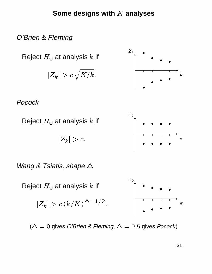
Some designs with K analyses

O’Brien & Fleming

Reject H0 at analysis k if

jZkj > cqK=k:

-

k

6Zk �

� � �

�� � �

Pocock

Reject H0 at analysis k if

jZkj > c:-

k

6Zk

� � � �

� � � �

Wang & Tsiatis, shape �

Reject H0 at analysis k if

jZkj > c (k=K)��1=2:-

k

6Zk

� � � �

� � � �

(�= 0 gives O’Brien & Fleming, �= 0:5 gives Pocock)

31

Example: cholesterol reduction trial

Properties of different designs

Sample sizes are per treatment.

Fixed sample size is 66.

K Maximum Expected sample sizesample size �=0 �=0:2 �=0:4

O’Brien & Fleming

2 67 67 65 565 68 68 64 50

10 69 68 64 48

Wang & Tsiatis, �= 0:25

2 68 67 64 525 71 70 65 47

10 72 71 64 44

Pocock

2 73 72 67 515 80 78 70 45

10 84 82 72 44

32

MONITORING

Implementing the OBF test

Divide the total sample size of 68 per treatment into 5

groups of roughly equal size, e.g.,

14 in groups 1 to 3, 13 in groups 4 and 5.

At analysis k, define

�X(k)A =

1

nAk

nAkXi=1

XAi; �X(k)B =

1

nBk

nBkXi=1

XBi

and

Zk =�X(k)A � �X

(k)Bq

�2(1=nAk +1=nBk):

Stop to reject H0 if

jZkj > 2:040q5=k; k = 1; : : : ;5:

Accept H0 if jZ5j < 2:040.

33

Implementing the 5-analysis OBF test

The stopping rule gives

type I error rate �= 0:050 and

power 0.902 at � = 0:4

if group sizes are equal to their design values.

Note the minor effects of discrete group sizes.

Perturbations in error rates also arise from small variations

in the actual group sizes.

For major departures from planned group sizes, we should

really follow the “error spending” approach — see later.

34

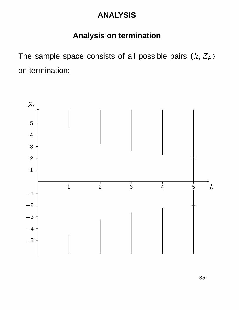
ANALYSIS

Analysis on termination

The sample space consists of all possible pairs (k; Zk)

on termination:

-

k1 2 3 4 5

6Zk

1

2

3

4

5

�1

�2

�3

�4

�5

35

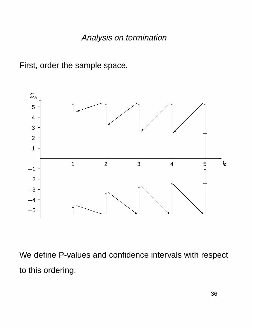
Analysis on termination

First, order the sample space.

-

k1 2 3 4 5

6Zk

1

2

3

4

5

�1

�2

�3

�4

�5

6

6

6

6

6

6

6

6

6

6

PPPPPPPq

�������)

ZZZZZZZZ~

��������=

@@@@@@@R

�������

@@@@@@@@R

��������

We define P-values and confidence intervals with respect

to this ordering.

36

The P-value for H0: �A = �B is the probability under H0

of observing such an extreme outcome.

-

k1 2 3 4 5

6Zk

1

2

3

4

5

�1

�2

�3

�4

�5

6

6

6

6

6

6

6

6

6

6

PPPPPPPq

�������)

ZZZZZZZZ~

��������=

@@@@@@@R

�������

@@@@@@@@R

���������

�

���

��

�����

����

��

��

E.g., if the test stops at analysis 3 with Z3 = 4:2, the

two-sided P-value is

Pr�=0fjZ1j � 4:56 or jZ2j � 3:23 or jZ3j � 4:2g

= 0:0013:

37

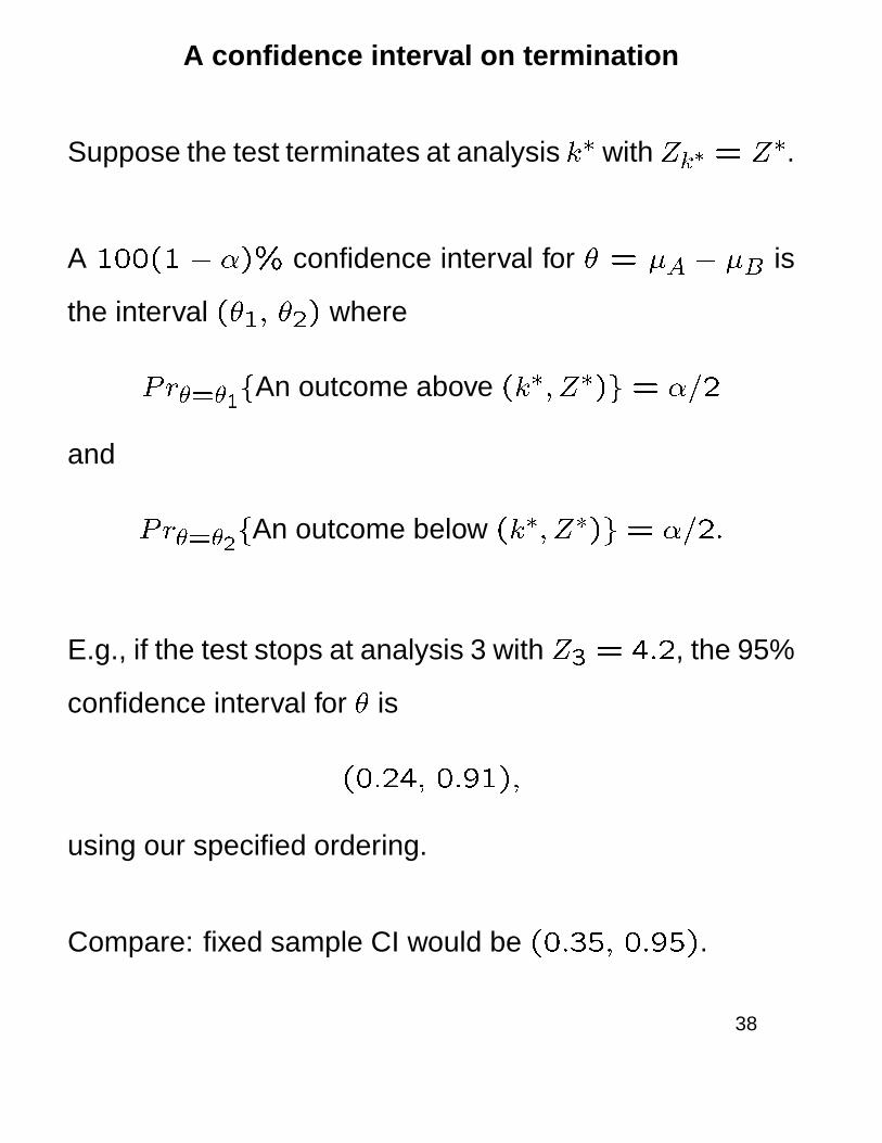
A confidence interval on termination

Suppose the test terminates at analysis k� with Zk� = Z�.

A 100(1 � �)% confidence interval for � = �A � �B is

the interval (�1; �2) where

Pr�=�1fAn outcome above (k�; Z�)g = �=2

and

Pr�=�2fAn outcome below (k�; Z�)g= �=2:

E.g., if the test stops at analysis 3 with Z3 = 4:2, the 95%

confidence interval for � is

(0:24; 0:91);

using our specified ordering.

Compare: fixed sample CI would be (0:35; 0:95).

38

9. Updating a design as a nuisance

parameter is estimated

The case of unknown variance

We can design as for the case of known variance but

use an estimate of �2 initially.

If in doubt, err towards over-estimating �2 in order to

safeguard the desired power.

At analysis k, estimate �2 by

s2k =

P(XAi � �X

(k)A )2+

P(XBi � �X

(k)B )2

nAk+ nBk � 2:

In place of Zk, define t-statistics

Tk =�X(k)A � �X

(k)Bq

s2k(1=nAk+1=nBk);

then test at the same significance level used for Zk when

�2 is known.

39

Updating the target sample size

Recall, maximum sample size is set to be the fixed sample

size multiplied by the Inflation Factor.

In a 5-group O’Brien & Fleming design for the cholesterol

example this is

1:026� f��1(1� �=2) +��1(1� �)g2 2�2=Æ2

= 134:8� �2:

After choosing the first group sizes using an initial estimate

of �2, at each analysis k = 1;2; : : : we can re-estimate

the target for nA5 and nB5 as

134:8� s2k

and modify future group sizes to achieve this.

40

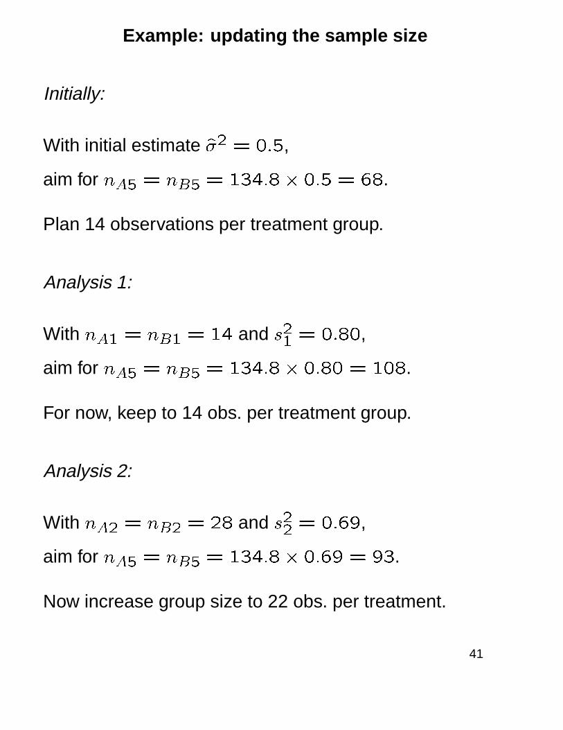
Example: updating the sample size

Initially:

With initial estimate �̂2 = 0:5,

aim for nA5 = nB5 = 134:8� 0:5 = 68.

Plan 14 observations per treatment group.

Analysis 1:

With nA1 = nB1 = 14 and s21= 0:80,

aim for nA5 = nB5 = 134:8� 0:80 = 108.

For now, keep to 14 obs. per treatment group.

Analysis 2:

With nA2 = nB2 = 28 and s22= 0:69,

aim for nA5 = nB5 = 134:8� 0:69 = 93.

Now increase group size to 22 obs. per treatment.

41

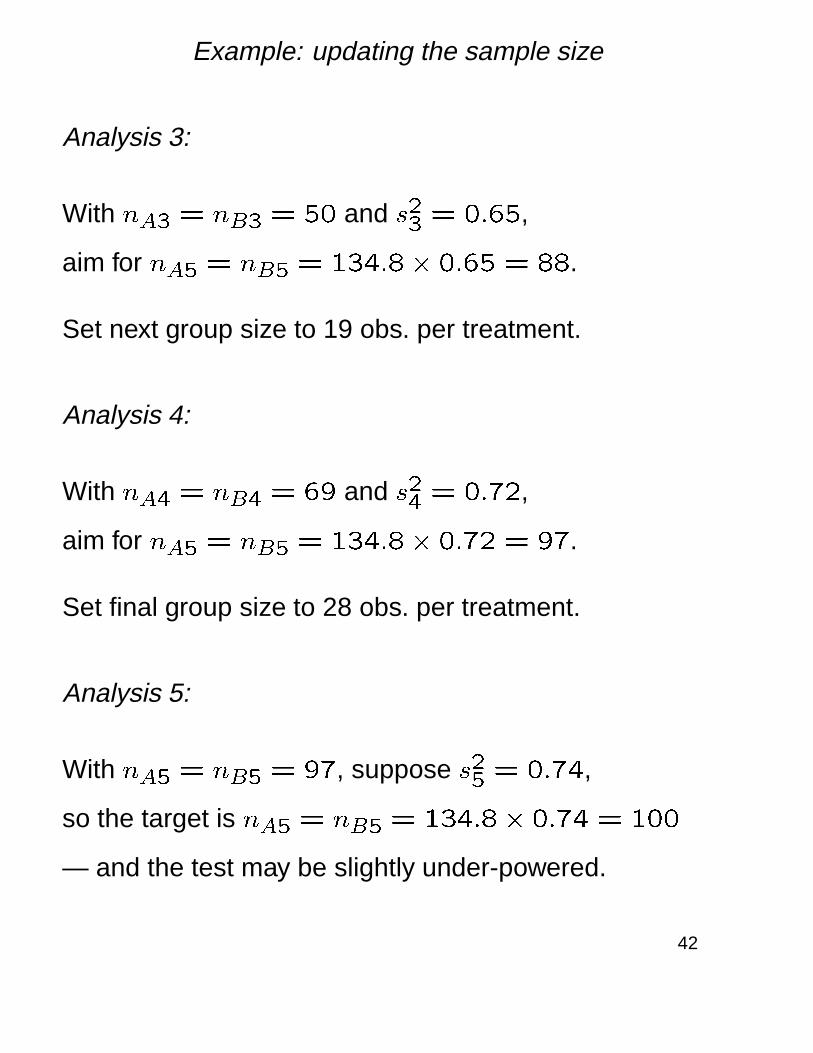
Example: updating the sample size

Analysis 3:

With nA3 = nB3 = 50 and s23= 0:65,

aim for nA5 = nB5 = 134:8� 0:65 = 88.

Set next group size to 19 obs. per treatment.

Analysis 4:

With nA4 = nB4 = 69 and s24= 0:72,

aim for nA5 = nB5 = 134:8� 0:72 = 97.

Set final group size to 28 obs. per treatment.

Analysis 5:

With nA5 = nB5 = 97, suppose s25= 0:74,

so the target is nA5 = nB5 = 134:8� 0:74 = 100

— and the test may be slightly under-powered.

42

Remarks on “re-estimating” sample size

The target information for � = �A � �B is

Imax = IF � f��1(1� �=2) +��1(1� �)g2 =Æ2

= 1:026� (1:960 + 1:282)2=0:42 = 67:4:

The relation between information and sample size

Ik =��

1

nAk+

1

nBk

��2��1

involves the unknown �2. Hence, the initial uncertainty

about the necessary sample size.

In effect, we proceed by monitoring observed information:

-�

I1

�

I2

�

I3

�

I4

�

I5

Imax

= 67:4

Information

NB, state Imax = 67:4 in the protocol, not n = : : :

43

Recapitulation

Designing a group sequential test:

� Formulate the testing problem

� Create a fixed sample study design

� Choose number of analyses and boundary shape

parameter

� Set maximum sample size equal to fixed sample size

times the inflation factor

Monitoring:

� Find observed information at each analysis

� Compare z-statistics with critical values

Analysis:

� P-value and confidence interval on termination

This method can be applied to many response

distributions and statistical models.

44

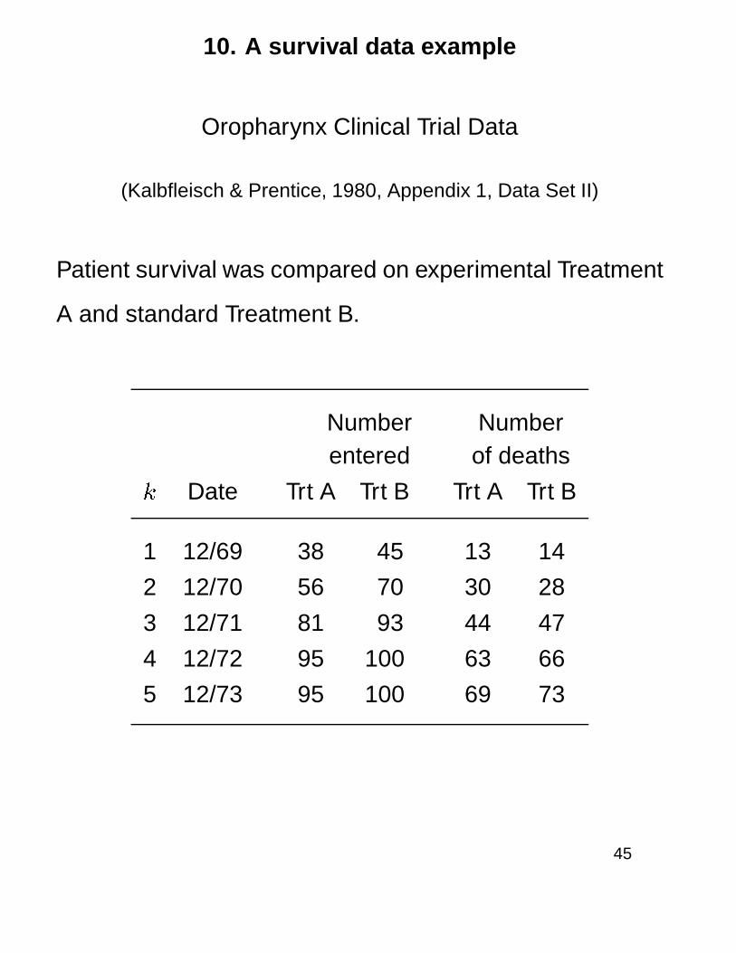
10. A survival data example

Oropharynx Clinical Trial Data

(Kalbfleisch & Prentice, 1980, Appendix 1, Data Set II)

Patient survival was compared on experimental Treatment

A and standard Treatment B.

Number Numberentered of deaths

k Date Trt A Trt B Trt A Trt B

1 12/69 38 45 13 14

2 12/70 56 70 30 28

3 12/71 81 93 44 47

4 12/72 95 100 63 66

5 12/73 95 100 69 73

45

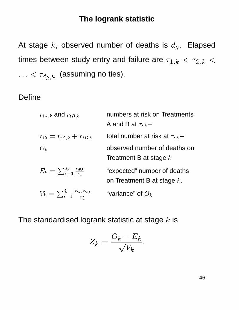
The logrank statistic

At stage k, observed number of deaths is dk. Elapsed

times between study entry and failure are �1;k < �2;k <

: : : < �dk;k (assuming no ties).

Define

riA;k and riB;k numbers at risk on Treatments

A and B at �i;k�

rik = riA;k + riB;k total number at risk at �i;k�

Ok observed number of deaths on

Treatment B at stage k

Ek =Pdk

i=1

riB;k

rik“expected” number of deaths

on Treatment B at stage k.

Vk =Pdk

i=1

riA;kriB;k

r2ik

“variance” of Ok

The standardised logrank statistic at stage k is

Zk =Ok � Ekp

Vk:

46

Proportional hazards model

Assume hazard rates hA on Treatment A and hB on

Treatment B are related by

hB(t) = �hA(t):

The log hazard ratio is � = ln(�).

Then, approximately,

Zk � N(�pIk; 1)

and

Cov(Zk1; Zk2) =p(Ik1=Ik2); 1 � k1 � k2 � K;

where Ik = Vk.

For � � 1, we have Ik � Vk � dk=4.

47

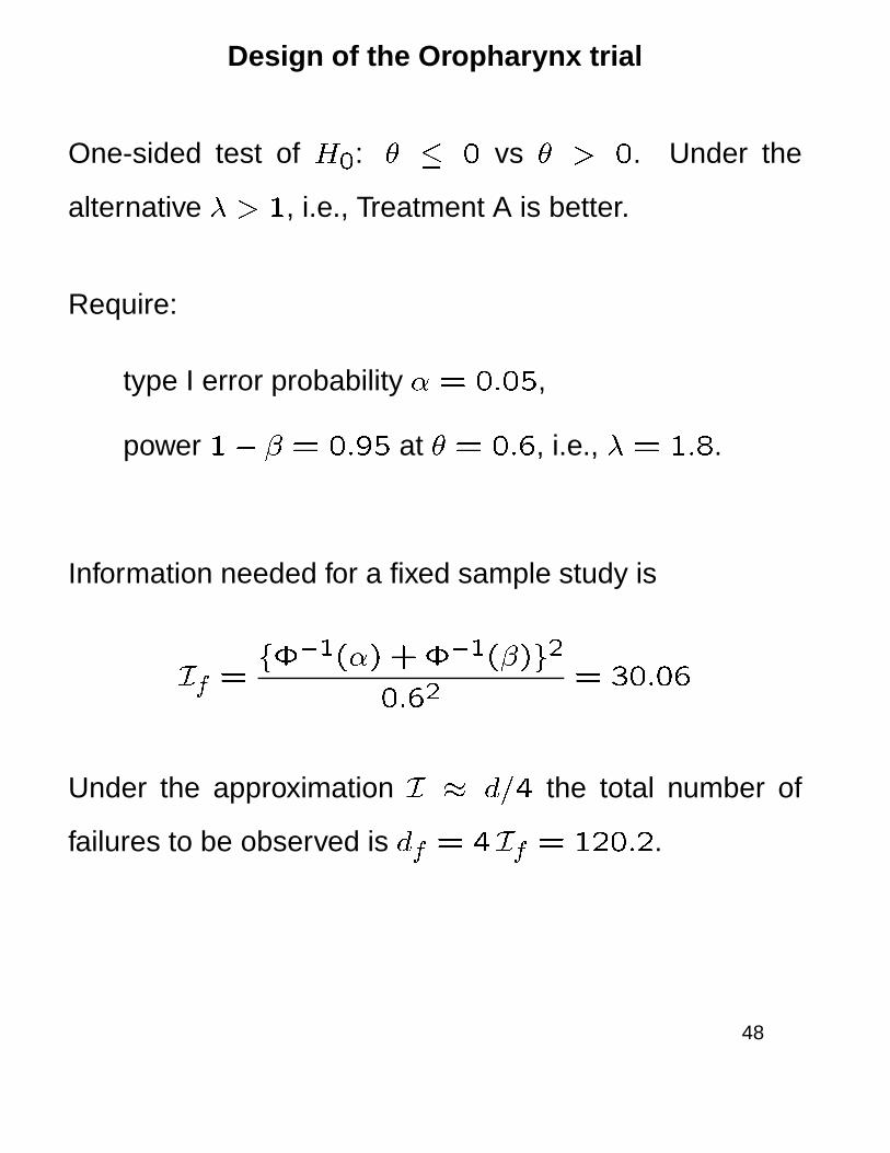
Design of the Oropharynx trial

One-sided test of H0: � � 0 vs � > 0. Under the

alternative � > 1, i.e., Treatment A is better.

Require:

type I error probability �= 0:05,

power 1� � = 0:95 at � = 0:6, i.e., � = 1:8.

Information needed for a fixed sample study is

If =f��1(�) +��1(�)g2

0:62= 30:06

Under the approximation I � d=4 the total number of

failures to be observed is df = 4 If = 120:2.

48

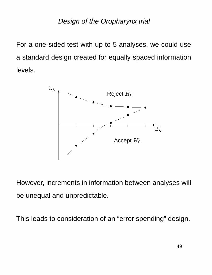
Design of the Oropharynx trial

For a one-sided test with up to 5 analyses, we could use

a standard design created for equally spaced information

levels.

-

Ik

6Zk

��

� � �

�

�

�

�

HH

PPP``̀

��

���

"""

!!!

!!!

Reject H0

Accept H0

However, increments in information between analyses will

be unequal and unpredictable.

This leads to consideration of an “error spending” design.

49

11. Error spending tests

Lan & DeMets (1983) presented two-sided tests which

“spend” type I error as a function of observed information.

Maximum information design:

Error spending function f(I)

-

IkImax

6f(I)

�

��!!�

"����#��#����"�!!��

Set the boundary at analysis k to give cumulative Type I

error f(Ik).

Accept H0 if Imax is reached without rejecting H0.

50

Error spending tests

Analysis 1:

Observed information I1.

Reject H0 if jZ1j > c1 where

Pr�=0fjZ1j > c1g= f(I1):

-

I1 k

6Zk

�

�

Analysis 2:

Cumulative information I2.

Reject H0 if jZ2j > c2 where

Pr�=0fjZ1j < c1; jZ2j > c2g

= f(I2)� f(I1):

-

I1 I2 k

6Zk

��

��

etc.

51

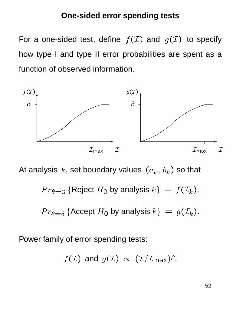
One-sided error spending tests

For a one-sided test, define f(I) and g(I) to specify

how type I and type II error probabilities are spent as a

function of observed information.

-

IImax

6f(I)

�

��!!�"

����������"�

!!��

-

IImax

6g(I)

�

��!!�"����������"�!!��

At analysis k, set boundary values (ak; bk) so that

Pr�=0 fReject H0 by analysis kg = f(Ik);

P r�=Æ fAccept H0 by analysis kg = g(Ik):

Power family of error spending tests:

f(I) and g(I) / (I=Imax)�.

52

One-sided error spending tests

1. Values fak; bkg are easily computed using iterative

formulae of McPherson, Armitage & Rowe (1969).

2. Computation of (ak; bk) does not depend on future

information levels, Ik+1;Ik+2; : : : .

3. In a “maximum information design”, the study

continues until the boundary is crossed or an analysis

is reached with Ik � Imax.

4. The value of Imax should be chosen so that

boundaries converge at the final analysis under a

typical sequence of information levels, e.g.,

Ik = (k=K) Imax; k = 1; : : : ;K:

53

Over-running

If one reaches IK > Imax , solving for aK and bK is

liable to give aK > bK .

-

k

6Zk

��

� � � bK

Æ aK

�

�

�

�

HH

PPP``̀

��

���

"""

"""

"""

........

Reject H0

Accept H0

Keeping bK as calculated guarantees type I error

probability of exactly �.

So, reduce aK to bK — and gain extra power.

Over-running may also occur if IK = Imax but the

information levels deviate from the equally spaced values

(say) used in choosing Imax.

54

Under-running

If a final information level IK < Imax is imposed, solving

for aK and bK is liable to give aK < bK .

-

k

6Zk

��

� � � bKÆ aK�

�

�

�

HH

PPP``̀

��

���

"""

!!!

(((........

Reject H0

Accept H0

Again, with bK as calculated, the type I error probability

is exactly �.

This time, increase aK to bK — and attained power will

be a little below 1� �.

55

A one-sided error spending design for

the Oropharynx trial

Specification:

one-sided test of H0: � � 0 vs � > 0,

type I error probability �= 0:05,

power 1� � = 0:95 at � = ln(�) = 0:6.

At the design stage, assume K = 5 equally spaced

information levels.

Use a power-family test with � = 2, i.e., error spent is

proportional to (I=Imax)2.

Information of a fixed sample test is inflated by a factor

R(K;�; �; �) = 1:101 (JT, Table 7.6).

So, we require Imax = 1:101 � 30:06 = 33:10, which

needs a total of 4� 33:10 = 132:4 deaths.

56

Summary data and critical values for the

Oropharynx trial

We construct error spending boundaries for the

information levels actually observed.

This gives boundary values (a1; b1); : : : ; (a5; b5) for the

standardised statistics Z1; : : : ; Z5.

Number Number

k entered of deaths Ik ak bk Zk

1 83 27 5.43 �1.60 3.00 �1.04

2 126 58 12.58 �0.37 2.49 �1.00

3 174 91 21.11 0.63 2.13 �1.21

4 195 129 30.55 1.51 1.81 �0.73

5 195 142 33.28 1.73 1.73 �0.87

This stopping rule would have led to termination at the

2nd analysis.

57

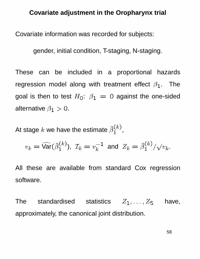
Covariate adjustment in the Oropharynx trial

Covariate information was recorded for subjects:

gender, initial condition, T-staging, N-staging.

These can be included in a proportional hazards

regression model along with treatment effect �1. The

goal is then to test H0: �1 = 0 against the one-sided

alternative �1 > 0.

At stage k we have the estimate �̂(k)1

,

vk =dVar(�̂(k)

1), Ik = v�1k and Zk = �̂

(k)1

=pvk.

All these are available from standard Cox regression

software.

The standardised statistics Z1; : : : ; Z5 have,

approximately, the canonical joint distribution.

58

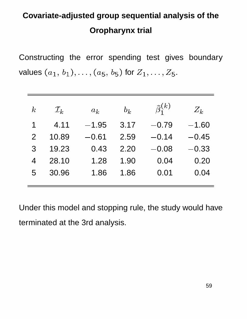
Covariate-adjusted group sequential analysis of the

Oropharynx trial

Constructing the error spending test gives boundary

values (a1; b1); : : : ; (a5; b5) for Z1; : : : ; Z5.

k Ik ak bk �̂(k)1

Zk

1 4.11 �1.95 3.17 �0.79 �1.60

2 10.89 �0.61 2.59 �0.14 �0.45

3 19.23 0.43 2.20 �0.08 �0.33

4 28.10 1.28 1.90 0.04 0.20

5 30.96 1.86 1.86 0.01 0.04

Under this model and stopping rule, the study would have

terminated at the 3rd analysis.

59

Further topics

Chapters of Jennison & Turnbull,

Group Sequential Methods with Applications

to Clinical Trials:

Ch 9. Repeated confidence intervals

Ch 10. Stochastic curtailment

Ch 12. Special methods for binary data

Ch 15. Multiple endpoints

Ch 16. Multi-armed trials

Ch 17. Adaptive treatment assignment

Ch 18. Bayesian approaches

Ch 19. Numerical computations for group

sequential tests

60