Embed Size (px)
Citation preview

ORIGINAL PAPER
Groundwater flow and residence time in a karst aquifer using ionand isotope characterization
M. A. Dıaz-Puga1 • A. Vallejos1 • F. Sola1 • L. Daniele2,3 • L. Molina1 •
A. Pulido-Bosch1
Received: 11 January 2016 / Revised: 4 July 2016 /Accepted: 17 August 2016 / Published online: 7 September 2016
� Islamic Azad University (IAU) 2016
Abstract In order to identify the origin of the main pro-
cesses that affect the composition of groundwater in a
karstic aquifer, a hydrogeochemical and isotopic study was
carried out of water from numerous observation wells
located in Sierra de Gador, a semiarid region in SE Spain.
Several natural and anthropogenic tracers were used to
calculate groundwater residence time within this complex
aquifer system. Analysis of major ions enabled the prin-
cipal geochemical processes occurring in the aquifer to be
established, and the samples were classified into four dis-
tinctive solute groups according to this criterion. Dissolu-
tion of carbonate rocks determines the chemical
composition of less mineralized water. In another group,
the concurrent dissolution of dolomite and precipitation of
calcite in gypsum-bearing carbonate aquifer, where the
dissolution of relatively soluble gypsum controls the
reaction, are the dominant processes. Marine intrusion
results in highly mineralized waters and leads to base
exchange reactions. The groundwater enrichment of minor
and trace elements allowed classification of the samples
into two classes that are linked to different flow patterns.
One of these classes is influenced by a slow and/or deep
regional flow, where the temperature is generally elevated.
The influence of sulphate reduces by up to 40 % the barium
concentration due to the barite precipitation. Isotope data
(T, 14C) confirm the existence of recent local flows, and
regional flow system, and ages of ground water may reach
8000 years. The importance of gypsum dissolution in this
aquifer is proved by the d34S content.
Keywords Karst � Hydrogeochemistry � Minor ions �Isotopes � Groundwater age
Introduction
Karstic carbonate massifs are complex aquifer mediums, in
which the circulation of recharge water occurs via frac-
tures, fissures, stratification and/or dissolution surfaces on
the rock. Along the flowpath, the chemistry of the water is
modified as a function of the materials it traverses due to
the water–rock interaction (Moral et al. 2008; Wu et al.
2009). Carbonate aquifers are particularly important in
semiarid, densely populated regions such as in the
Mediterranean Basin, where they can account for 50 % of
the water resources that supply its population (Margat
2008; Caetano Bicalho et al. 2012). Overexploitation of
groundwater can lead to a change in its hydrogeochemical
characteristics, generally leading to a deterioration in water
quality due to processes such as salinization through dis-
solution of evaporites (Reynauld et al. 1999; Martos-
Rosillo and Moral 2015; Vallejos et al. 2015a), or marine
intrusion processes (Terzic et al. 2008; Sdao et al. 2012).
The carbonate massif of Sierra de Gador comprises the
principal recharge area for the aquifer that has developed
beneath this mountain range, as well as for the whole of its
southern extension, which lies beneath the coastal plain of
Campo de Dalias. The latter represents one of the main
Editorial responsibility: J. Trogl.
& A. Vallejos
1 Department of Hydrogeology, University of Almerıa, 04120
Almerıa, Spain
2 Department of Geology, FCFM, University of Chile,
Santiago, Chile
3 Andean Geothermal Center of Excellence (CEGA), Fondap-
Conicyt, Santiago, Chile
123
Int. J. Environ. Sci. Technol. (2016) 13:2579–2596
DOI 10.1007/s13762-016-1094-0
areas of fruit and vegetable production in the whole of
Europe, with a surface area under greenhouse cultivation
exceeding 20,000 ha. The pronounced overexploitation of
its groundwaters for irrigation and urban water supply has
provoked a marked fall in piezometric levels, in addition to
an advance in the saline front that has caused water
salinization in some areas (Daniele et al. 2013a; Vallejos
et al. 2015b). The structural complexity of this extensive
aquifer system, combined with its lithological variability
and the presence of numerous mineralizations dispersed
across a fair proportion of its surface area (Daniele et al.
2013b), means that the physicochemistry of its ground-
waters cover a wide range.
Various hydrochemical tools can be used to understand
the processes that cause the chemical enrichment of the
groundwaters (Sanchez et al. 2015). Hydrogeochemical
and isotope analyses can additionally help to construct a
conceptual model of the hydrogeological functioning of the
aquifer with greater precision (Barbieri et al. 2005). Major,
minor and trace ions can be very useful in identifying
groundwater mixing or rock–water interactions, as well as
in characterizing groundwater flows (Gimenez-Forcada and
Vega-Alegre 2015). The major ions allow differentiation of
the most important causal processes of the bulk of the
chemical load carried in the water, which arises from the
interaction of the aqueous flow with the main lithological
components of the aquifer medium. However, to under-
stand the processes in more detail, it is necessary to turn to
the minor ions. Thus, the concentration of ions like Ba or
Sr will be controlled by the solubility of the barite and
celestite, respectively (Hanor 2004; Underwood et al.
2009). Natural uranium present relates to the mobilization
of this element from minerals and rocks that form the
aquifer or adjacent geological formations (Liesch et al.
2015). For most of the minor elements (i.e. Li, F, Ti, V, Cr,
Ni, Cu, Zn, As, Br, Rb, I and Cs), the high concentrations
are related to high salinity waters, which are representative
of the deep circulation inside the carbonate-evaporite
aquifer (Morgantini et al. 2009). These aquifers are char-
acterized by the presence of carbonate rocks (dolostone and
limestone) with interlayers of more soluble mineral phases
(e.g. anhydrite, gypsum and minor halite and fluorite) and
are often confined under a low permeability cover (Chio-
dini et al. 1995). Groundwater circulation in the deep
aquifer is generally characterized by long residence times.
Radiogenic isotopes like 3H or 14C allow the mean resi-
dence times of the water in the aquifer to be determined
(Xanke et al. 2015)—using tritium for periods of less than
60 years (Gonfiantini et al. 1998) and 14C for older waters
(Plummer 2005).
The purpose of this study was to determine the principal
hydrogeochemical processes occurring in the Sierra de
Gador aquifer, as well as the residence time of its waters.
To this end, we analysed the ionic ratios of certain major,
minor and trace ions and the values of stable and
radioactive isotopes (July 2009). Additionally, the geo-
chemistry of certain minor elements (e.g. barium, rubid-
ium, uranium, caesium) supplies extra information on the
coexistence of groundwater flows with different chemical
compositions.
Hydrogeological setting
The study was carried out in the Sierra de Gador, situated
in the province of Almeria in the extreme southeast of
Spain (Fig. 1). The surface area of this coastal mountain
chain is close to 1000 km2. The climate is Mediterranean,
characterized by warm, dry summers and mild winters. The
amount of water available depends on the rainfall regime—
and it rains seldom and irregularly. The semiarid character
of the area arises due to the combination of a lack of
precipitation (400 mm on the southern slopes of Sierra de
Gador), strong insolation (around 2900 h year-1), inter-
annual variability in precipitation (22–35 %) and high
potential evaporation (about 900 mm year-1). Tempera-
ture increases from a mean of 16 �C on the top of the
mountains to 18.7 �C at the foot. January is the coldest
month (10 �C), and August is the hottest (27.2 �C) (Martın-
Rosales et al. 2007). The inflows feeding the aquifers are
basically infiltration from rainfall over the unit, as well as
runoff from the slopes of the Sierra de Gador. Current
outflows are almost exclusively the result of pumped
abstractions.
Geologically, it belongs to the Internal Zones of the
Betic Cordillera (Alpujarride Complex). The structure of
the Alpujarride Complex is characterized by the superpo-
sition of a number of tectonic units or nappes. The entire
superimposed nappe structure has been subject to impor-
tant tensional and strike-slip events (Sanz de Galdeano
et al. 1985), which have led to the development of basins,
now filled with Neogene and Quaternary detrital material.
Two tectonic units have been identified in the area:
Gador and Felix. The Gador unit consists of a basal layer of
phyllite with quartzite intercalations, which has been
assigned to the Permian–Triassic. The transition from this
underlying formation to the limestone-dolomite layer
above is usually a layer of calcoschist and marly limestone
(Martin-Rojas et al. 2009). The upper part of the series is
dolomitic, with limestone predominating towards the top.
The whole series is approximately 1000 m thick. The
formations of the Felix unit, like those of the Gador one,
consist of a basal metapellitic layer with a carbonate layer
above. The carbonate layer is much thinner than its Gador
counterpart, normally less than 100 m. It is also Middle-
Upper Triassic in age. The Gador unit covers almost all the
2580 Int. J. Environ. Sci. Technol. (2016) 13:2579–2596
123
whole of Sierra de Gador, exposing small klippen of the
overlying Felix unit.
Above these materials are the Miocene deposits, made
up of calcarenite in the outcropping sectors, and marl and
gypsum beneath a Plioquaternary infill (Rodrıguez-Fer-
nandez and Martın-Penela 1993). Quaternary deposits are
present along the whole of the base of the southern face of
the Sierra, making up large alluvial fans that occasionally
exceed 150 m in thickness. In the western sector, the Berja
intra-mountain basin is filled with Neogene and Quaternary
deposits. The carbonates of the Gador and Felix units are
highly permeable. The schist, phyllite and quartzite of both
Alpujarride units are practically impermeable. With respect
to the post-orogenic materials, the Miocene and Pliocene
calcarenite and the Quaternary materials are also perme-
able. The Sierra de Gador aquifers are geometrically
complex as a consequence of the intense alpine compres-
sional tectonics of the region.
Numerous reconnaissance boreholes have provided
evidence of their structural complexity by revealing the
variable thicknesses of Quaternary materials and the
faulting, which has resulted in substantial vertical and
horizontal compartmentalization of the carbonate rocks.
Materials and methods
A sampling survey was carried out to monitor water quality
and assess the main physicochemical processes in this
aquifer. In July 2009, 78 samples of groundwater were
collected from springs and wells (Fig. 1). The springs of
Sierra de Gador show high discharge variability (70 % of
the springs less than 5 L/s and the rest 20–100 L/s). The
wells have a varying depth, between a few and a hundred of
metres. Temperature, electrical conductivity (EC) and pH
were determined in situ. Alkalinity (as HCO3) was deter-
mined by titration at the time of sampling. Samples were
taken in duplicate, filtered using a 0.45-lm Millipore filter
and stored in polyethylene bottles at 4 �C. For cation anal-
ysis, one bottle of each sample was acidified to pH\ 2 with
environmental grade (ultra-pure) nitric acid to avoid prob-
lems of absorption or precipitation (Vallejos et al. 2015b).
Sample composition was determined by means of an ICP-
Mass Spectrometer at Acme Labs (Vancouver, Canada).
The analytical results obtained are summarized in Table 1.
The mineral saturation indices (SI) indicate the degree of
saturation in a particular mineral phase compared to the
aqueous solution in contact. Based on this SI value, the trend
of precipitation or dilution of the mineral phases can be
deduced. The SI was obtained using the PHREEQC code,
version 3 (Parkhurst and Appelo 2013). According to the
characteristics of the study plot, the phases analysed were
calcite, dolomite, gypsum and halite (Vallejos et al. 2015b).
d34SSO4, d18OSO4 and d18OH2O isotope measurements
were determined at the Stable Isotope Laboratory of the
Zaidin Experimental Station (Granada, Spain). The pre-
treatment of samples for isotope analysis d34S and d18Ofrom SO4 implies to convert the sulphate to BaSO4 by the
addition of barium chloride. Firstly, it was necessary to
acidify the samples with HCl, to get the pH below 3.5. In
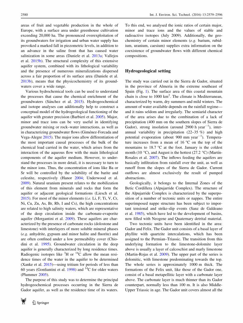
Fig. 1 Location of the study area and sampling points in different colours according to the groups identified. 1 cross section; 2 fault; 3 thrust
fault; 4 well; 5 spring; 6 marine intrusion area
Int. J. Environ. Sci. Technol. (2016) 13:2579–2596 2581
123

Table 1 Results of chemical analyses of water samples
Sample Group Class T EC pH Cl SO4 HCO3 Na Mg Ca K Br
(8C) lS/cm mg/L
1 G4 A 26 1549 7.44 405.6 64.2 250.1 138.1 66.0 79.8 3.6 0.10
2 G4 A 25.4 1115 7.55 240.3 61.5 256.2 83.2 52.2 67.5 2.9 0.06
3 G2-B A 25.3 782 7.88 71.1 76.1 292.8 40.9 39.5 63.7 2.7 0.04
4 G2-B A 24.1 827 7.53 123.2 59.1 286.7 49.4 44.2 63.1 3.0 0.05
5 G4 A 27.4 1080 7.71 228.3 53.5 286.7 101.4 42.9 55.4 5.6 0.06
6 G4 A 24.2 1040 7.85 183.3 41.3 250.1 53.3 49.5 75.6 2.0 0.05
7 G2-B B 22.8 557 7.7 31.0 42.7 280.6 17.6 32.7 54.2 1.2 0.03
8 G2-B A 24.2 670 7.54 96.1 38.7 256.2 34.1 38.0 51.2 2.7 0.03
9 G2 B 21.8 403 7.66 27.0 20.1 207.4 12.8 25.2 38.8 1.0 0.02
10 G2 B 21.6 460 7.72 43.1 19.0 219.6 21.0 26.5 41.6 1.0 0.02
11 G2-B B 21.5 419 7.63 27.0 20.9 219.6 13.6 26.5 41.4 1.0 0.08
12 G2-B B 20.9 459 7.6 32.0 18.2 237.9 15.4 28.4 45.9 0.9 0.03
13 G2-B B 20.5 453 7.56 28.0 25.2 244.0 13.8 29.3 44.8 0.9 0.03
14 G2-B A 26.1 502 7.44 21.0 35.0 280.6 12.1 35.1 50.3 1.9 0.02
15 G2-B B 22.8 548 7.62 33.0 33.8 298.9 16.3 30.0 54.4 5.3 0.02
16 G2 A 22.7 570 7.46 26.0 50.9 298.9 13.8 38.6 57.9 1.8 0.03
17 G2 A 23.3 664 7.64 60.1 40.5 280.6 27.6 35.6 53.1 6.6 0.02
18 G4 B 21.5 1046 7.91 229.3 40.2 256.2 71.1 41.0 80.0 1.3 0.02
19 G4 A 20.7 1579 7.58 329.5 57.7 256.2 140.0 47.8 105.3 6.0 0.05
20 G3 B 22.5 1072 7.35 211.3 50.6 305.0 66.5 46.8 86.3 1.3 0.30
21 G4 A 15.9 3380 7.49 784.1 98.7 213.5 396.6 78.8 148.4 3.1 0.56
22 G1 B 16.8 541 7.42 26.0 8.8 347.6 10.4 27.9 69.9 0.7 0.13
23 G3 B 17.3 326 8.17 11.0 6.0 195.2 6.8 25.5 31.4 0.3 0.33
24 G2 B 18.9 449 7.7 22.0 36.2 250.1 11.9 25.6 48.3 5.1 0.11
25 G2 B 16.3 390 7.76 12.0 7.8 262.3 6.8 29.5 40.2 0.5 0.18
26 G2 B 17.4 394 7.8 17.0 19.6 268.4 8.3 30.5 36.0 0.5 0.11
27 G4 A 22.6 2930 7.55 761.1 292.3 317.1 371.3 95.5 114.4 6.9 0.12
28 G4 A 27.8 1266 7.55 256.4 89.5 317.1 152.6 45.7 44.9 9.3 0.09
29 G1 A 42.5 915 7.03 19.0 217.3 384.2 19.4 42.6 123.5 4.2 0.07
30 G1 A 30.9 932 7.36 15.0 224.7 445.2 8.9 47.7 127.4 9.5 0.11
31 G1 A 28.9 839 7.19 15.0 140.6 445.2 10.7 49.3 105.3 6.9 0.08
32 G2 A 22.7 939 6.98 25.0 92.7 616.0 9.4 70.3 124.7 4.6 0.22
33 G1 A 22.7 980 7.08 16.0 120.6 561.1 8.3 62.2 129.6 1.2 0.08
34 G1 A 24.1 967 7.01 12.0 182.1 512.3 7.4 59.8 122.7 3.1 0.06
35 G2-B B 18.2 561 7.55 10.0 34.9 378.1 4.9 35.0 63.2 3.6 0.08
36 G2-B A 20.1 599 7.68 10.0 54.3 365.9 6.8 39.3 70.6 1.0 0.07
37 G1 B 16.7 538 8.44 9.0 79.7 283.6 6.2 30.0 77.5 0.9 0.05
38 G1 A 19.1 765 7.85 17.0 170.9 347.6 15.3 36.0 115.0 1.0 0.06
39 G1 B 15.2 368 7.58 6.0 61.6 189.1 3.7 16.4 54.7 2.5 0.03
40 G1 B 12.1 259 8.18 4.0 3.5 219.6 1.4 17.9 30.9 0.3 0.09
41 G2 B 14.4 271 7.97 7.0 13.4 161.7 3.2 17.9 30.9 0.5 0.04
42 G1 A 23.2 859 7.16 17.0 179.9 414.7 17.9 52.3 113.2 2.7 0.17
43 G2 A 20.6 676 7.95 24.0 112.7 305.0 23.3 38.6 75.2 1.6 0.04
44 G3 A 24.1 740 8.71 45.1 152.4 247.0 41.3 38.0 72.7 3.2 0.02
45 G1 B 8.9 301 8.07 3.0 17.6 189.1 1.4 14.9 38.7 2.5 0.08
46 G1 B 17.1 345 8.42 5.0 65.5 164.7 3.7 19.7 38.0 0.5 0.07
47 G2 B 17.8 356 8.12 9.0 42.3 207.4 7.4 23.5 42.0 0.5 0.23
2582 Int. J. Environ. Sci. Technol. (2016) 13:2579–2596
123

Table 1 continued
Sample Group Class T EC pH Cl SO4 HCO3 Na Mg Ca K Br
(8C) lS/cm mg/L
48 G2 A 23.4 844 7.41 43.1 122.3 372.0 29.1 53.6 72.5 3.9 0.07
49 G2 B 23.7 384 8.43 8.0 33.3 201.3 7.4 22.6 41.3 0.3 0.04
50 G1 B 16.7 483 8.09 7.0 108.3 201.3 2.7 27.1 58.5 3.6 0.06
51 G1 B 16.7 302 7.93 5.0 10.7 213.5 2.0 20.0 35.9 0.4 0.07
52 G2 B 15.2 300 8.13 5.0 13.1 231.8 1.8 20.4 35.3 0.5 0.72
53 G2 B 20.6 536 7.75 14.0 82.3 244.0 11.4 30.2 55.2 1.4 0.05
54 G4 A 24.1 1735 7.4 347.5 72.4 286.7 142.9 60.0 114.2 2.2 0.10
55 G1 B 18.5 553 7.71 6.0 132.1 207.4 4.2 26.0 61.1 2.2 0.10
56 G1 B 18 557 7.87 8.0 141.3 207.4 3.5 30.1 71.6 4.7 0.26
57 G1 B 17.1 542 7.85 10.0 135.6 201.3 3.7 33.2 70.7 0.8 0.31
58 G2 B 17.9 611 7.69 15.0 125.8 237.9 14.2 34.0 67.1 0.9 0.31
59 G2 A 21.1 1072 7.47 52.1 127.4 396.4 40.4 74.7 76.2 3.1 0.29
60 G4 B 20.3 761 7.47 16.0 168.2 359.8 11.5 42.9 91.0 5.1 0.23
61 G1 B 20.3 734 7.52 14.0 172.8 280.6 9.4 41.3 88.7 5.4 0.23
62 G3 B 20.3 1479 7.26 42.1 456.9 115.9 22.9 125.1 139.4 16.0 0.61
63 G3 A 24.2 1428 7.46 126.2 321.1 341.5 62.2 84.6 123.5 3.4 0.36
64 G3 A 22.4 1464 7.48 153.2 183.1 291.5 22.0 62.0 86.7 55.2 0.57
65 G3 A 22.7 1228 7.34 109.2 218.0 323.2 67.7 67.1 96.6 4.2 0.13
66 G3 A 21.9 1155 7.45 106.1 214.3 268.4 64.9 56.5 98.5 5.2 0.07
67 G3 B 20.1 1556 7.27 65.1 515.1 372.0 32.4 116.0 161.8 6.9 0.67
68 G3 B 21.5 1478 7.3 47.1 364.5 402.5 33.4 107.6 158.4 3.8 1.46
69 G3 B 19.2 2260 7.18 121.2 664.1 463.5 48.4 191.0 216.3 7.9 0.86
70 G3 B 20.4 1782 7.17 68.1 490.8 463.5 43.5 135.5 183.3 6.6 0.80
71 G3 B 19.7 1853 7.23 70.1 464.6 475.7 45.3 144.7 183.2 5.3 0.69
72 G3 B 20.2 1701 7.1 75.1 509.1 445.2 39.4 128.7 183.0 3.4 0.80
73 G3 B 20.3 974 7.5 30.0 213.4 320.2 26.9 61.7 105.7 5.8 1.18
74 G3 A 24.4 2530 8.01 369.5 565.6 341.5 230.0 80.9 252.7 8.2 3.18
75 G2 B 16.5 415 6.62 16.0 20.9 237.9 10.7 26.8 31.3 4.2 2.75
76 G2 B 18.3 329 8.05 11.0 13.0 201.3 4.5 19.5 31.1 4.2 0.67
77 G2 B 17.9 343 8.3 13.0 21.6 195.2 5.9 26.2 21.4 5.0 1.27
78 G2 B 20.3 331 9.12 16.0 16.0 201.3 6.4 20.4 27.8 7.1 0.07
SW 15.3 55.000 8.32 21,308.0 3426.0 35.4 13,584.0 1564.0 468.0 412.0 73.0
Sample Ba Cs Li Rb Si Sr U Saturation index
lg/L Barite Celestite Gypsum
1 202 1.0 9.2 2.6 5651 1763 3.2 0.29 -1.86 -1.93
2 153 0.7 8.9 2.0 5604 1392 3.3 0.23 -1.93 -1.95
3 85 0.5 8.4 1.9 5920 1258 3.9 0.11 -1.83 -1.84
4 135 0.8 7.0 1.8 5903 1230 3.6 0.22 -1.96 -1.96
5 124 1.7 18.2 3.8 7546 1897 1.4 0.12 -1.83 -2.08
6 265 0.5 4.8 1.6 6050 874 2.0 0.33 -2.27 -2.06
7 112 0.3 2.7 0.7 5265 542 2.8 0.09 -2.39 -2.1
8 107 1.0 8.1 2.1 6128 855 2.0 -0.02 -2.25 -2.19
9 196 0.2 1.7 0.5 4486 264 1.4 0.09 -2.97 -2.5
10 202 0.2 4.7 0.5 4359 277 1.5 0.07 -2.98 -2.51
11 185 0.2 1.9 0.5 4581 285 1.4 0.09 -2.93 -2.47
12 193 0.3 1.9 0.5 4672 255 1.8 -0.03 -3.05 -2.5
Int. J. Environ. Sci. Technol. (2016) 13:2579–2596 2583
123

Table 1 continued
Sample Ba Cs Li Rb Si Sr U Saturation index
lg/L Barite Celestite Gypsum
13 170 0.2 4.0 0.5 4592 249 1.6 0.13 -2.92 -2.37
14 124 0.5 5.1 1.6 5999 657 1.2 0 -2.39 -2.22
15 150 0.3 2.6 0.8 5100 280 2.4 0.13 -2.77 -2.19
16 88 0.4 4.5 1.4 5674 504 1.5 0.05 -2.37 -2.01
17 61 0.1 4.9 2.2 5464 425 2.1 -0.22 -2.53 -2.14
18 220 0.4 3.0 0.9 4540 495 2.4 0.3 -2.54 -2.04
19 183 0.5 3.7 1.2 4421 548 2.9 0.32 -2.4 -1.82
20 231 0.3 3.8 0.8 5111 530 2.8 0.38 -2.43 -1.93
21 262 0.4 3.8 1.2 3359 466 1.5 0.65 -2.38 -1.57
22 21 0.0 1.4 0.3 3527 173 0.7 -0.76 -2.81 -2.2
23 9 0.0 0.7 0.1 3761 38 0.1 -1.64 -4.28 -3..09
24 45 0.0 0.8 0.8 2933 87 0.3 -0.27 -3.22 -2..18
25 28 0.0 0.7 0.1 3294 46 0.3 -1.05 -4.14 -2.9
26 34 0.0 1.6 0.1 3923 79 0.6 -0.6 -3.52 -2.55
27 80 0.5 11.9 4.0 6321 944 4.9 0.41 -1.64 -1.26
28 80 1.0 25.8 5.3 6136 687 3.8 0.06 -2.08 -1.97
29 61 18.9 63.1 13.6 13.740 2548 2.3 0.03 -1.16 -1.21
30 37 9.2 23.2 7.5 8572 2700 1.6 -0.02 -1.14 -1.19
31 53 6.0 25.4 6.3 7557 1896 2.6 0.01 -1.44 -1.43
32 85 1.4 13.6 2.1 5916 1194 4.4 0.12 -1.89 -1.58
33 52 1.6 10.8 2.1 6027 1447 3.6 0.02 -1.69 -1.44
34 41 2.0 11.5 2.8 5736 1697 2.3 0.04 -1.44 -1.29
35 94 0.3 2.4 0.9 4279 223 2.5 0 -2.88 -2.13
36 65 0.6 4.5 1.1 4234 338 2.8 -0.03 -2.53 -1.92
37 40 0.1 4.2 0.5 4050 744 1.6 -0.02 -2.01 -1.69
38 59 0.0 6.4 0.5 10.076 902 2.5 0.33 -1.68 -1.28
39 65 0.0 3.1 0.5 4395 785 1.1 0.17 -2 -1.86
40 14 0.0 0.3 0.1 1586 61 0.2 -1.58 -4.3 -3.29
41 48 0.0 1.1 0.1 3401 227 0.5 -0.49 -3.15 -2.71
42 38 2.1 26.8 3.5 5797 1831 3.4 0.07 -1.4 -1.31
43 39 0.1 20.0 0.7 5445 936 2.5 0.01 -1.8 -1.6
44 36 0.3 89.6 1.9 6146 1064 3.2 0 -1.62 -1.51
45 26 0.0 4.6 0.4 3191 198 0.4 -0.54 -3.07 -2.48
46 45 0.0 1.0 0.2 3673 508 0.5 0.03 -2.16 -1.99
47 47 0.0 1.8 0.3 3808 571 0.9 -0.15 -2.31 -2.15
48 37 0.9 18.6 4.3 5461 1817 3.9 -0.07 -1.51 -1.62
49 48 0.0 1.5 0.2 3892 400 0.7 -0.33 -2.56 -2.27
50 34 0.0 1.5 0.4 3530 915 2.8 0.06 -1.76 -1.65
51 111 0.0 0.7 0.2 3452 303 1.5 -0.29 -3.14 -2.77
52 188 0.0 0.8 0.3 3508 481 1.4 0.06 -2.85 -2.69
53 45 0.1 2.8 0.4 4668 770 2.2 0 -1.95 -1.8
54 87 0.4 5.5 1.3 5026 863 2.8 0 -2.14 -1.73
55 34 0.0 2.1 0.4 3459 1440 2.5 0.04 -1.5 -1.56
56 38 0.2 2.8 0.6 4059 1566 2.8 0.15 -1.44 -1.48
57 36 0.0 2.7 0.4 4149 1653 3.0 0.12 -1.44 -1.51
58 52 0.1 3.5 0.5 4495 1348 2.6 0.25 -1.69 -1.56
59 104 0.4 10.8 1.7 6931 1062 4.3 0.38 -1.77 -1.62
2584 Int. J. Environ. Sci. Technol. (2016) 13:2579–2596
123

this way, the co-precipitation of others barium salts is
avoided. d18OH2O determination was carried out using a Gas
Bench II Analyses (GC-IRMS), d34SSO4 with a Fisons NA
1500 NC elemental analyser and d18OSO4 using a thermal
conversion elemental analyser (Thermo Finnigan TC/EA).
The analytical uncertainties (1r) for d34S, d18OSO4 and
d18OH2O are ±0.1, ±0.5 and ±0.2 %, respectively.
Forty-three groundwater samples were collected for 3H
analysis in 1 L high-density polyethylene bottles. The
samples were analysed at the University of Miami Tritium
Laboratory (USA). Tritium was measured by internal Gas
Proportional Counting of H2 gas made from the water
sample. Low-level water samples go through an elec-
trolytic enrichment step whereby tritium concentrations are
increased about 60-fold by means of volume reduction.
Accuracy of the low-level measurement with enrichment is
0.10 TU (0.3 pCi L-1 of H2O, Vallejos et al. 2015b).
In addition, eight measurements of 14C activity with d13Cwere available. These samples were analysed at Hertelendi
Laboratory of Environmental Studies (Debrecen, Hungary).
The 14C activities were measured by precipitation of TDIC
in the form of BaCO3. The volume of the sampling con-
tainer is usually 60 l, which is sufficient for extracting about
2.5 g of carbon from water with a concentration of about
250 ppm of bicarbonates. BaCl2 solution is added to the
water sample after adjusting the pH to convert all bicar-
bonates to carbonates (carbon-free concentrated NaOH is
added until pH reaches about 8.5). Normally such a pre-
cipitate is fine grained and requires a day to settle com-
pletely. Carbon dioxide is evolved from the precipitate by
adding concentrated H2SO4 or H3PO4. The chemically pre-
treated sample is combusted or acid digested CO2 being
obtained in a controlled oxygen stream. Gaseous impurities
are removed by passing the produced CO2 through a hot
copper furnace. The purified CO2 is trapped into stainless
steel vessel and measured by gas proportional counting. The
precision was ±0.5 % pMC for 14C activities.
Results and discussion
Major constituents
The chemical composition of groundwater samples along
Sierra de Gador shows the complexity of this aquifer sys-
tem is mainly determined by its lithology. In order to
characterize the hydrochemistry of the groundwater based
on major ions, the analytical data were plotted on a mod-
ified Durov diagram (Fig. 2). In this diagram, the cation
and anion triangles are recognized and separated along the
Table 1 continued
Sample Ba Cs Li Rb Si Sr U Saturation index
lg/L Barite Celestite Gypsum
60 58 0.1 4.1 1.0 4604 2077 3.7 0.31 -1.32 -1.38
61 57 0.1 4.0 1.2 4840 1975 3.6 0.26 -1.32 -1.37
62 68 0.2 9.4 2.4 6296 3382 7.0 0.57 -0.85 -0.94
63 45 15.1 148.9 10.6 6450 3295 6.7 0.24 -1.11 -1.11
64 50 17.2 105.3 12.2 6022 3084 8.8 0.19 -1.16 -1.42
65 53 18.6 94.3 11.7 6356 3295 8.4 0.25 -1.07 -1.31
66 64 18.3 101.0 12.2 6142 3507 7.9 0.33 -1.04 -1..3
67 71 0.0 9.1 1.5 7059 3810 7.0 0.62 -0.77 -0.85
68 49 0.1 12.0 0.6 7172 2878 7.0 0.32 -1.03 -0.99
69 67 0.0 19.3 0.6 9378 5075 10.9 0.63 -0.65 -0.72
70 50 0.1 13.3 0.5 7780 3164 8.2 0.42 -0.91 -0.85
71 63 0.0 15.2 0.7 8508 3616 9.1 0.51 -0.88 -0.87
72 42 3.0 15.3 4.9 10.561 4581 9.5 0.34 -0.72 -0.83
73 65 0.0 7.1 1.0 5655 2164 4.9 0.36 -1.24 -1.26
74 36 64.5 553.8 42.0 6232 5708 6.3 0.23 -0.63 -0.69
75 25 0.0 3.2 0.4 4025 146 2.3 -0.67 -3.18 -2.56
76 28 0.0 1.3 0.2 4118 112 0.4 -0.79 -3.49 -2.74
77 30 0.0 1.7 0.4 3935 102 0.8 -0.58 -3.32 -2.7
78 19 0.0 1.3 0.3 4060 234 0.6 -0.97 -3.09 -2.75
SW 19 0.0 0.2 131 500 8.45 3.2
EC electrical conductivity. Location of sampling points in Fig. 1
Int. J. Environ. Sci. Technol. (2016) 13:2579–2596 2585
123

25 % axes so that the main field is conveniently divided
into nine subfields (Al-Bassam et al. 1997; Al-Bassam and
Khalil 2012). Four groups can be recognized according to
the data distribution on this graph. These groups were
identified as G-1, G-2, G-3 and G-4. Group G-1 is char-
acterized by calcium bicarbonate samples with low min-
eralization. G-2 contains samples that are more magnesic
than G-1, apparently affected by a process of dolomite
dissolution. The calcium–magnesium–bicarbonate facies
from groups (G-1 and G-2) indicates recharge from lime-
stone and dolostone, main rock of this aquifer system.
Group 3 shows the influence of sulphate dissolution, and
samples have a higher saline content than in G-1 or G-2.
G-4 contains the samples with the highest saline content,
some of which have a sodium chloride facies. This fact,
and their proximity to the coast, could indicate that these
samples are affected by marine intrusion.
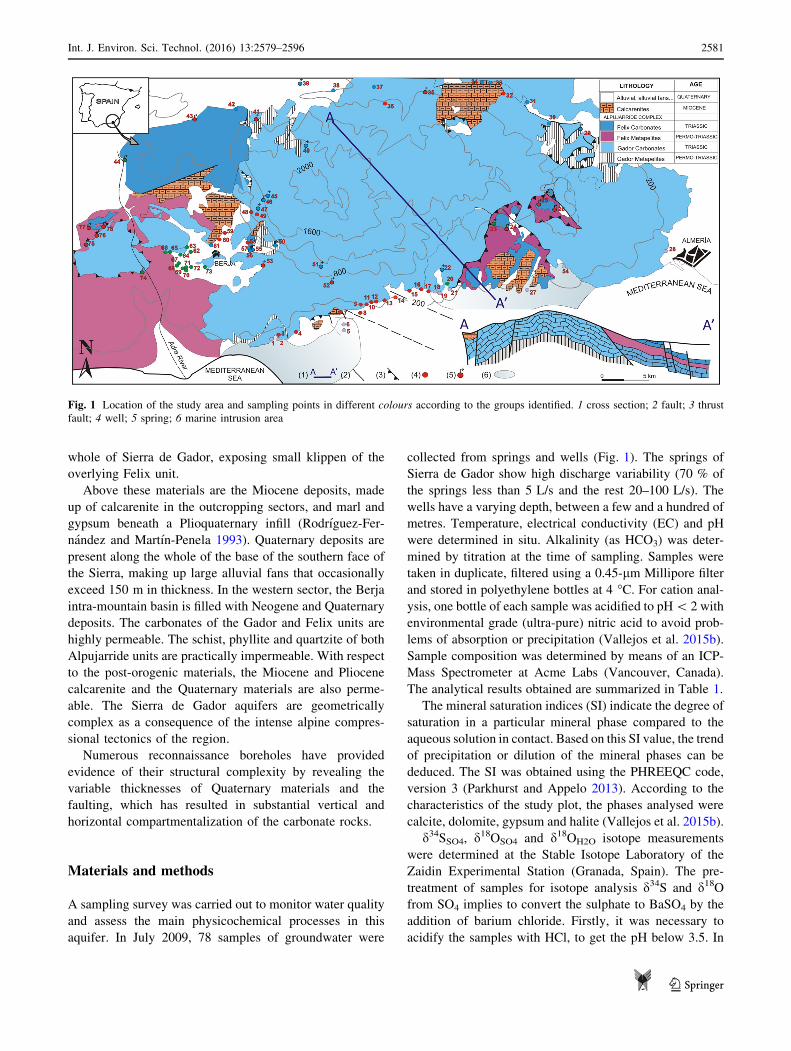
The relationships among some major ions were studied
with the goal of recognizing the main hydrogeochemical
processes that affect the defined groups. Figure 3a shows
the relationship for HCO3 versus Ca ? Mg-SO4. This
relationship reveals the carbonate dissolution processes
excluding the influence of sulphate. The 1:1 line depicts the
dolomite dissolution processes. Samples from G-1 and G-2
are distributed along this straight line, while those from
G-3 and G-4 are above the line. In order to determine the
sulphate influence, the HCO3 ? SO4 versus Ca ? Mg
graph was used (Fig. 3b). In this case, samples from G-1,
G-2 and G-3 are on the 1:1 line showing that the carbonate
and sulphate dissolution are the dominant processes
affecting these samples. The sulphate influence on samples
in G-3 is remarkable. On the other side, samples in G-4
show an excess in Ca or Mg linked to an additional con-
tribution of Mg due to marine processes. The marine
influence on G-4 samples can be determined thanks to the
graph Cl vs. Br (Fig. 3c), being the distribution of G-4
samples close to the line defined by Cl/Br seawater ratio
(Vengosh et al. 1999).
Figure 3d, which shows the relationship between Mg
and HCO3, clarifies which processes determine the ion
distribution of the samples. A ratio of 1:2 indicates con-
gruent dissolution of dolomite. Groups G-1 and G-2 are
slightly about this ratio. Nevertheless, samples in group
G-3 clearly have an excess of magnesium. The process that
could explain this is dedolomitization. An excess of dis-
solved calcium is produced as a consequence of the
Fig. 2 Expanded Durov
diagram corresponding to
groundwater samples
2586 Int. J. Environ. Sci. Technol. (2016) 13:2579–2596
123
dissolution of gypsum; it provokes the precipitation of
calcite, so increasing the quantity of dissolved magnesium
(Back et al. 1983; Deike 1990; Saunders and Toran 1994;
Ma et al. 2011). The net result is that the dissolution of
gypsum induces the transformation of dolomite to calcite in
the rock and produces waters with increased Mg2?.
Approximately 95 % of the SI values for calcite and
dolomite in the groundwater samples were greater than
zero (Vallejos et al. 2015b).
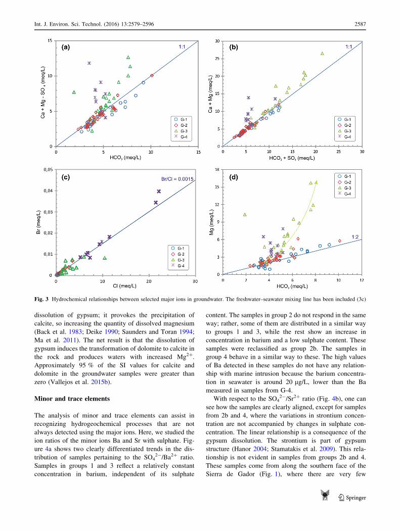
Minor and trace elements
The analysis of minor and trace elements can assist in
recognizing hydrogeochemical processes that are not
always detected using the major ions. Here, we studied the
ion ratios of the minor ions Ba and Sr with sulphate. Fig-
ure 4a shows two clearly differentiated trends in the dis-
tribution of samples pertaining to the SO42-/Ba2? ratio.
Samples in groups 1 and 3 reflect a relatively constant
concentration in barium, independent of its sulphate
content. The samples in group 2 do not respond in the same
way; rather, some of them are distributed in a similar way
to groups 1 and 3, while the rest show an increase in
concentration in barium and a low sulphate content. These
samples were reclassified as group 2b. The samples in
group 4 behave in a similar way to these. The high values
of Ba detected in these samples do not have any relation-
ship with marine intrusion because the barium concentra-
tion in seawater is around 20 lg/L, lower than the Ba
measured in samples from G-4.
With respect to the SO42-/Sr2? ratio (Fig. 4b), one can
see how the samples are clearly aligned, except for samples
from 2b and 4, where the variations in strontium concen-
tration are not accompanied by changes in sulphate con-
centration. The linear relationship is a consequence of the
gypsum dissolution. The strontium is part of gypsum
structure (Hanor 2004; Stamatakis et al. 2009). This rela-
tionship is not evident in samples from groups 2b and 4.
These samples come from along the southern face of the
Sierra de Gador (Fig. 1), where there are very few
Fig. 3 Hydrochemical relationships between selected major ions in groundwater. The freshwater–seawater mixing line has been included (3c)
Int. J. Environ. Sci. Technol. (2016) 13:2579–2596 2587
123
intercalated gypsums within the limestone, hence the low
sulphate concentrations in the samples. The increment in
strontium would be linked to a longer residence time of this
water, which increases the concentration of this ion in
dissolution. Something similar occurs with barium. The
increment in barium observed in these samples is not
related to their sulphate concentration. The samples
belonging to these groups were taken from deep boreholes
where the flow was probably part of a slow, regional flow;
this would favour concentration in these ions. In turn,
samples in groups 1, 2 and 3 had higher sulphate and lower
barium concentrations. These low concentrations of barium
would be a result of barite precipitation. An increase in
sulphate favours saturation in barite and its precipitation, so
that the concentration of dissolved barium is reduced
(Underwood et al. 2009; Gimenez-Forcada and Vega-
Alegre 2015).
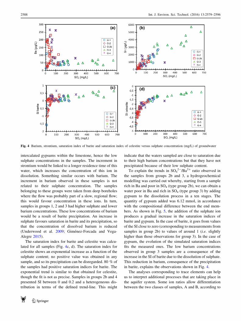
The saturation index for barite and celestite was calcu-
lated for all samples (Fig. 4c, d). The saturation index for
celestite shows an exponential increase as a function of the
sulphate content; no positive value was obtained in any
sample, and so its precipitation can be disregarded. 80 % of
the samples had positive saturation indices for barite. The
exponential trend is similar to that obtained for celestite,
though the fit is not as precise. Samples in groups 2b and 4
presented SI between 0 and 0.2 and a heterogeneous dis-
tribution in terms of the defined trend-line. This might
indicate that the waters sampled are close to saturation due
to their high barium concentrations but that they have not
precipitated because of their low sulphate content.
To explain the trends in SO42-/Ba2? ratio observed in
the samples from groups 2b and 3, a hydrogeochemical
modelling was carried out whereby, starting from a sample
rich in Ba and poor in SO4 (type group 2b), we can obtain a
water poor in Ba and rich in SO4 (type group 3) by adding
gypsum to the dissolution process in a ten stages. The
quantity of gypsum added was 6.12 mmol, in accordance
with the compositional difference between the end mem-
bers. As shown in Fig. 5, the addition of the sulphate ion
produces a gradual increase in the saturation indices of
barite and gypsum. In the case of barite, it goes from values
of the SI close to zero (corresponding to measurements from
samples in group 2b) to values of around 1 (i.e. slightly
higher than those observations for group 3). In the case of
gypsum, the evolution of the simulated saturation indices
fits the measured ones. The low barium concentrations
observed in group 3 samples are a consequence of the
increase in the SI of barite due to the dissolution of sulphate.
This reduction in barium, consequence of the precipitation
in barite, explains the observations shown in Fig. 4.
The analyses corresponding to trace elements can help
us to interpret additional processes that are taking place in
the aquifer system. Some ion ratios allow differentiation
between the two classes of samples, A and B, according to
Fig. 4 Barium, strontium, saturation index of barite and saturation index of celestite versus sulphate concentration (mg/L) of groundwater
2588 Int. J. Environ. Sci. Technol. (2016) 13:2579–2596
123

two well defined trends (Fig. 6). These trends can be
observed in the Rb/Sr ratio (Fig. 6a), where Rb concen-
tration increases according to an exponential distribution
function with respect to Sr (class A) and, in contrast, where
the Rb values remain constant and independent of the Sr
concentration (class B). In terms of the U/Li ratio, samples
in class B were positively aligned in accordance with the
increase in both uranium and lithium concentrations.
Nevertheless, the samples classified as A do not exhibit any
relationship existing between these two ions (Fig. 6b).
These different patterns of enrichment in trace ions in the
two classes could be linked to contrasting flow patterns.
The samples belonging to class A—which show higher
rates of ionic enrichment in trace elements than in class
B—could be determined by slower and/or deeper flowpaths
that are more regional in nature, i.e. covering greater dis-
tances. In general, these samples had higher temperatures
than the corresponding samples from class B (Table 1).
The concentrations in uranium in the analysed samples
showed a highly significant correlation with silica for class
B (Fig. 6c). This would be an indicator that the bulk of the
uranium has a detritic source. In fact, the samples with the
highest uranium concentrations ([7 lg/L) were taken from
boreholes in the Berja basin (Fig. 1), where detritic sedi-
ments overlie the Triassic carbonates. The samples in class
A do not show this correlation, probably as a consequence
of the thermal character of these waters, which favours the
mobilization of these ions (Valentino and Stanzione 2003).
The effect of temperature in the class A samples is par-
ticularly obvious for ions like Rb and Cs, causing them to
be mobilized and incorporated into the groundwater.
Figure 6d shows how the increase in such ions in samples
of class A is linear above a concentration of 5 lg/L in Rb,
while it is practically nil for the remainder of the samples
in this class and in class B.
The differentiation of samples into two classes, A and B,
established from the ion ratios between certain minor and
trace ions was utilized to see whether the behaviour in
groups 1, 2, 3 and 4, established from the ion ratios of the
major ions, is homogeneous. The criterion to distinguish
the classes A and B has been only geochemical. Never-
theless, there is a clear correlation between class A and
deep samples and class B and shallow samples, due to the
fact these classes are differentiated by their regional
character and residence time. Classes A and B are condi-
tioned by temperature and by the velocity and length of the
flowpath. With the aim of discovering whether these fac-
tors condition the major ion content of the groundwaters,
we plotted graphs of SO4 vs. Ca and HCO3 vs. Mg, which
identify the various groups subdivided according to whe-
ther they belong to class A or B (Fig. 7). Group 4 is not
included in either graph given that external processes
(marine intrusion) affect the ionic content of certain ions
like Mg, as well as temperature, so masking any other
processes occurring. Figure 7a shows that the established
groups can be differentiated by looking at the class to
which they belong. The differentiation between classes A
and B is clear for the samples belonging to group 1, and
this is also true for samples in group 2. In both groups,
samples in class A exhibit higher ion concentrations than
samples in class B; this is explained by a more effective
dissolution as a consequence of the more regional character
of the flows and the higher temperatures. Samples in group
3 also show a different distribution between A and B.
However, in this case, the ion concentrations of the sam-
ples belonging to class B are higher than in class A.
Samples belonging to 3-B were taken from boreholes in a
part of the carbonate aquifer overlain by detritic deposits,
with abundant intercalated layers of gypsum. The results
obtained based on the HCO3/Mg ratio (Fig. 7b) are very
similar. There is a good differentiation between groups 1
and 2 belonging to classes A and B, though this is not true
for the samples in group 3. In this case, the 3-B samples
have higher sulphate concentrations, since they are affected
more by a dedolomitization process, which in the end leads
to a greater enrichment in bicarbonate and magnesium.
Isotopic composition of groundwater
Sulphur isotopes of sulphate (d34S and d18O)
The use of several isotopes, coupled with hydrogeological
and hydrochemical information, has proved to be a useful
tool for assessing the origin of solutes. Krouse (1980)
Fig. 5 Comparison between barite and gypsum saturation indices
obtained with measured and simulated water versus sulphate
concentration (mg/L). The simulated data were obtained from an
initial sample, adding gypsum in ten steps
Int. J. Environ. Sci. Technol. (2016) 13:2579–2596 2589
123

suggested that d34S is useful for identifying natural and
anthropogenic sources of dissolved sulphate. In the area
studied, the d34S-SO4 values ranged from -2.8 to 20.6 %,
while d18O-SO4 values ranged between 2.5 and 16.1 %(Fig. 8a; Table 1). According to these data, any direct
anthropogenic impact on SO4 concentrations (sewage,
fertilizers) can be excluded. Therefore, the study of the
source of the SO4 focussed on natural sources such as
pyrite oxidation and gypsum dissolution. Figure 8a shows
the mixing processes affecting d34S from gypsum disso-
lution and sulphide oxidation. The influence of seawater is
not significant due to the low percentage of seawater in
groundwater samples. Regarding natural sources, the d34S-SO4 values of Triassic sulphates are between ?15.1 and
?16 % for d34S and between ?10.8 and ?16.3 % for
d18O (Ortı et al. 2014), while the d34S-SO4 of sulphides is
between ?0.4 and ?2.6 % for d34S and between 0 and
?5 % for d18O (Arribas and Arribas 1995; Garcıa-Lorenzo
et al. 2014). The majority of the samples are related to a
gypsum dissolution exceeding 40 %. This linear relation-
ship—where the top end is in the region associated with
evaporites and the bottom end can be extrapolated into the
region associated with sulphide-mineral oxidation—has
also been observed at a mining site in an arid climate in the
Monument Valley site, Arizona (Miau et al. Miao et al.
2013). Very few of the samples collected (Fig. 8b) lie
within the sulphide oxidation field defined by Van Stem-
pvoort and Krouse (1994), which is the zone where the
Fig. 6 Hydrochemical relationships between selected minor ions in groundwater. The trend-line of the samples is shown
Fig. 7 (a) SO4/Ca and (b) HCO3/Mg ratios. All data are in meq/L. The samples have been classified in groups (G1 to G3) and classes (A and B)
2590 Int. J. Environ. Sci. Technol. (2016) 13:2579–2596
123

isotope data would be plotted if the oxygen of sulphate and
water were in isotopic equilibrium. High values of d18O of
sulphate indicate the influence from gypsum/anhydrite
dissolution or mixing with such waters.
Tritium and carbon-14 isotopes
Of the 43 samples analysed for 3H, 21 samples contained no3H above the detection limit of 0.1 TU (Table 1). This
indicates these 21 samples are likely to bemore than 60 years
old. Most of the groundwaters with no measured 3H were
from the northern and southern Sierra de Gador. The maxi-
mum value was 5.77 TU, indicating that the contribution of
rainfall to the groundwater recharge during the last years is
very low. Values of[4 TU correspond to areas of klippen
and some contact springs on the upper part of the mountain,
where groundwater can be considered shallow.
Rb was used to identify the main trends in tritium
content, since the concentration of this ion shows a clear
relationship with the flowpath and the residence time; thus,
samples with short flowpaths have a Rb concentration of
around 0 lg/L (class B), whereas the Rb concentration
increases in samples corresponding to regional flows
(Fig. 6a). Samples classified as A and B according to minor
and trace elements were plotted on a graph of Rb vs. tri-
tium (Fig. 9). Most of the samples from class A have low
tritium values of less than 1 TU and variable concentrations
in Rb. Three samples in this class had tritium concentra-
tions in excess of 1 TU. These samples are affected by
marine intrusion (group 4), and, in this case, the tritium
content comes from the seawater mixing, which is a recent
water (Yechieli et al. 2001; Sivan et al. 2005). Samples
belonging to class B have a very low Rb content and
variable tritium. However, two groups of samples can be
recognized by looking at their tritium concentration.
Samples with a concentration of more than 4 TU would
come from faster-flowing groundwater flowpaths, while
concentrations of less than 3 TU show longer residence
times and can be identified with an intermediate flow
(Fig. 9).
The ages of the samples were determined using the
carbonate dissolution correction-factor calculation pro-
posed by Fontes and Garnier (1979) based on their d13C and14C content. This method was selected because it requires
the fewest parameter estimates. For calculation purposes,
certain values had to be assumed since they were not
measured: these included d13CCO2 = -17 %, a value
obtained for areas with a semiarid climate (Rightmire 1967;
Kunkler 1969); d13Ccarb = 1.4 %, taken from data mea-
sured in a carbonate aquifer from northern France (Fontes
Fig. 8 (a) Plot of d34S-SO4 versus d34S-H2O. Gypsum values are
taken from Ortı et al. (2014) and sulphide values from Arribas and
Arribas (1995) and Garcıa-Lorenzo et al. (2014). Rainwater values are
taken from Bottrell et al. (2008) and seawater values from Hosono
et al. (2011). (b) Plot of d18O-H2O versus d18O-SO4. The shaded area
corresponds to the isotopic sulphide oxidation zone defined by Van
Stempvoort and Krouse (1994)
Fig. 9 Rb (lg/L) versus T (TU). The samples have been plotted
according to classes A and B
Int. J. Environ. Sci. Technol. (2016) 13:2579–2596 2591
123

Table 2 Results of isotopic analyses of water samples
Sample Group Class T d34S d18OSO4 d18OH2O14C d13C Age
TU ±1r % % PMC ±1r % Ka
1 G4 A
2 G4 A 1.50 0.09 12 7.8 -7.6 35 0.17 - M
3 G2-B A 0.30 0.09 12 8.3 -8.1
4 G2-B A 0.00 0.09 9.6 7.8 -8.1
5 G4 A 0.00 0.09 9.9 7.7 -8.3 10 0.05 -6 7.9
6 G4 A 0.53 0.09
7 G2-B B 0.07 0.09 11 4 -8.2
8 G2-B A 0.00 0.09 9.4 6.7 -8.2 22 0.11 -7 5.4
9 G2 B
10 G2 B
11 G2-B B 10 5.9 -8.1
12 G2-B B 0.10 0.09 8.1 5.8 -8.2
13 G2-B B 0.00 0.09 10 7.8 -8.1 42 0.21 -9 3.6
14 G2-B A 0.00 0.09 5.2 6.7 -8.4
15 G2-B B 0.05 0.09 11 8.8 -8.3 28 0.14 -7 1.8
16 G2 A 0.00 0.09
17 G2 A 0.09 0.09 6.5 8.6 -8.2
18 G4 B 2.39 0.09
19 G4 A 0.00 0.09 14 8 -8.9
20 G3 B 1.00 0.09
21 G4 A 4.79 0.12 60 0.30 -8 M
22 G1 B 2.43 0.10 8.4 4.8 -7.5
23 G3 B 5.17 0.12
24 G2 B 4.31 0.12 12 9.5 -7.3
25 G2 B 2.51 0.10
26 G2 B 5.77 0.12 6.8 6.6 -7.3
27 G4 A 0.15 0.09 5.4 6.2 -6.3 34 0.17 -7 1.0
28 G4 A 12 8.8 -6.6
29 G1 A 3.6 16.1 -8.4
30 G1 A 13 8.5 -7.6
31 G1 A 11 10.2 -8.4
32 G2 A
33 G1 A 10 8.2 -8.4
34 G1 A 4.1 11.1 -8.5
35 G2-B B -2.8 10.5 -8.4
36 G2-B A 0.8 2.5 -8.1
37 G1 B 9.3 8.4 -8.9
38 G1 A
39 G1 B 14 11 -9
40 G1 B 5.05 0.12
41 G2 B 12 8.2 -8.8
42 G1 A 14 11.5 -8.6
43 G2 A 5.6 6.5 -8.4
44 G3 A 10 7.1 -8
45 G1 B 10 4.1 -6.9
46 G1 B 2.56 0.10 16 13 -7.9
47 G2 B 1.93 0.09
2592 Int. J. Environ. Sci. Technol. (2016) 13:2579–2596
123

and Garnier 1979); the 14C activity of the soil CO2 (Ag) was
taken as 100 pmC and the 14C activity of solid (Ac) as 0
pmC. Certain values had to be calculated, including the
concentration of carbon of inorganic origin from ion bal-
ance; the concentration of total dissolved carbon was taken
to be that defined by Mook (1976), and the isotope frac-
tionation factor was calculated from Emrich et al. (1970) for
the corresponding groundwater temperature.
Using this information, the value of initial 14C activities
can be calculated. Substituting these data into the
radioactive decay equation yields a mean age for the water
samples. The results show that, in general, the waters in the
carbonate rocks of the Sierra de Gador are several thousand
years old (Tables 1 and 2). The tritium content indicates
that, in some cases, this water is mixed with more recent
water. They correspond to the sectors closest to the coast,
where the effects of sea water intrusion are seen.
Figure 10 shows a conceptual model of the study area,
where the relationship between groundwater flow, hydro-
geochemical processes and transit time is summarized.
Conclusions
The hydrochemical and isotopic study of the Sierra de
Gador aquifer macrosystem has enabled us to recognize a
series of processes that explains the chemical differentia-
tion of its waters. The major ion ratios reveal the main
Table 2 continued
Sample Group Class T d34S d18OSO4 d18OH2O14C d13C Age
TU ±1r % % PMC ±1r % Ka
48 G2 A 14 9.2 -7.7
49 G2 B 1.50 0.09
50 G1 B 0.90 0.09 16 13.5 -9.6
51 G1 B 0.92 0.09
52 G2 B 0.55 0.09
53 G2 B 0.67 0.09 14 9.6 -8.3
54 G4 A 1.43 0.09 12 7.8 -8.2 42 0.21 -8 2.1
55 G1 B 0.69 0.09 15 11.5 -9.6
56 G1 B 0.77 0.09 16 11.5 -9.6
57 G1 B
58 G2 B 13 10.8 -9
59 G2 A
60 G4 B 0.68 0.09
61 G1 B 15 12.1 -9.6
62 G3 B 11 8.4 -9.1
63 G3 A 0.63 0.09 21 8.4 -9.3
64 G3 A 12 8.6 -8.4
65 G3 A 12 8.8 -8.5
66 G3 A 0.47 0.09 13 9.6 -8.4
67 G3 B 12 7.8 -8.3
68 G3 B 10 7.3 -8.8
69 G3 B 10 5.5 -7.4
70 G3 B 10 6.8 -6.9
71 G3 B 10 7.3 -8
72 G3 B
73 G3 B 1.00 0.09
74 G3 A 2.47 0.09 15 12 -8.5
75 G2 B 5.07 0.12
76 G2 B 4.66 0.12
77 G2 B 4.42 0.12
78 G2 B 4.41 0.12 11 8.8 -7.1
SW 2.3 0.1 1.06
Location of sampling points in Fig. 1 (M: modern water)
Int. J. Environ. Sci. Technol. (2016) 13:2579–2596 2593
123

causal processes of the mineralization of the waters sam-
pled, classifying them into four groups according to their
composition (G1 to G4). These processes are: (1) dissolu-
tion of limestone, (2) dissolution of dolomite, (3) dissolu-
tion of evaporites, (4) mixing with seawater. Nevertheless,
small changes in composition in the minor ions allowed us
to recognize some hydrogeochemical processes. The con-
tent of Ba and Sr is controlled by sulphate concentration. In
the case of Ba, as sulphate increases, so does the SI of the
barite, which markedly reduces the barium concentration
due to the precipitation of barite. For its part, the Sr con-
centration of many of the samples was proportional to the
sulphate concentration, which is a clear indicator that the
Sr forms part of the structure of the gypsum mineralization.
Another reason for the increase in certain minor ions is the
residence time of water in the aquifer. The samples were
classified into two classes (A and B) according to their
content in minor ions. Class A corresponded to samples
taken from deep boreholes that tapped waters with a long
and slow flowpath through the aquifer and which, in some
cases, had a higher temperature. Their concentrations of
Rb, Cs and U were markedly higher than those in class B.
In turn, samples in class B came from springs or shallow
boreholes, with shorter residence times. In these, the U/Si
ratio showed a linear increase, which indicates that the U
comes from the leaching of the detritic deposits.
The study of the radioactive isotopes T and 14C cor-
roborated the apparent residence times of the water in the
aquifer. The values of TU in waters in class B generally
exceeded 1 TU, indicating a short transit time. On the other
hand, class A comprised samples with TUs of less than 1
TU, with the exception of those affected by marine intru-
sion (in which case the mixing with recent seawater
increased the tritium content). The activity of 14C led to
estimates of age of between 2 and 8 ky for samples in this
class.
Acknowledgments This work takes part of the general research lines
promoted by the CEI-MAR Campus of International Excellence as a
joint initiative between the universities of Almeria, Granada, Huelva
and Malaga, headed by the University of Cadiz. This work was
supported by the Andalusia Regional Government, Spain, through the
Excellence Research Project P06-RNM-01696 and by MINECO-
FEDER, through Project CGL2015-67273-R.
References
Al-Bassam AM, Khalil AR (2012) DurovPwin: a new version to plot
the expanded Durov diagram for hydro-chemical data analysis.
Comput Geosci 42:1–6
Al-Bassam AM, Awad HS, Al-Alawi JA (1997) DurovPlot a
computer program for processing and plotting hydro-chemical
data. Groundwater 35(2):362–367
Arribas A, Arribas A (1995) Caracteres metalogenicos y geoquımica
isotopica del azufre y el plomo de los yacimientos de minerales
metalicos del Sureste de Espana. Boletın Geologico y Minero
106(1):23–62
Back W, Hanshaw BB, Plummer LN, Rahn PH, Rightmire CT, Rubin
M (1983) Process and rate of dedolomitization: mass transfer and14C dating in a regional carbonate aquifer. Geol Soc Am Bull
94:1415–1429
Barbieri M, Boschetti T, Petitta M, Tallini M (2005) Stable isotope
(2H, 18O and 87Sr/86Sr) and hydrochemistry monitoring for
groundwater hydrodynamics analysis in a karst aquifer (Gran
Sasso, central Italy). Appl Geochem 20:2063–2081
Fig. 10 Scheme of
hydrogeochemical processes,
groundwater flow and transit
time in Sierra de Gador aquifer
system based on (a) major ions,
(b) minor ions and (c) isotopes.G1 to G4 correspond to the
different established groups, A
and B are the defined classes,
and T is the tritium content. The
groundwater age has also been
indicated
2594 Int. J. Environ. Sci. Technol. (2016) 13:2579–2596
123

Bottrell S, Tellam J, Bartlett R, Hughes A (2008) Isotopic compo-
sition of sulfate as a tracer of natural and anthropogenic
influences on groundwater geochemistry in an urban sandstone
aquifer, Birmingham, UK. Appl Geochem 23:2382–2394
Caetano Bicalho C, Batiot-Guilhe C, Seidel JL, Van Exter S, Jourde
H (2012) Geochemical evidence of water source characterization
and hydrodynamic responses in a karst aquifer. J Hydrol
450–451:206–218
Chiodini G, Frondini F, Marini L (1995) Theoretical geothermome-
ters and pCO2 indicators for aqueous solution coming from
hydrothermal systems of medium-low temperature hosted in
carbonate–evaporite rocks. Application to the thermal springs of
the Etruscan Swell, Italy. Appl Geochem 10:337–346
Daniele L, Vallejos A, Corbella M, Molina L, Pulido-Bosch A
(2013a) Geochemical simulations to assess water–rock interac-
tions in complex carbonate aquifers: the case of Aguadulce (SE
Spain). Appl Geochem 29:43–54
Daniele L, Corbella M, Vallejos A, Diaz-Puga M, Pulido-Bosch A
(2013b) Geochemical simulations to assess the fluorine origin in
Sierra de Gador groundwater. J Geofluids 13(2):221–231
Deike RG (1990) Dolomite dissolution rates and possible Holocene
dedolomitization of water-bearing units in the Edwards aquifer,
South-Central Texas. J Hydrol 112:335–373
Emrich K, Ehhalt D, Vogel JC (1970) Carbon isotope fractionation
during the precipitation of calcium carbonate. Earth Planet Sci
Lett 8:363–371
Fontes JC, Garnier JM (1979) Determination of the initial 14C activity
of the total dissolved carbon: a review of the existing models and
a new approach. Water Resour Res 15(2):399–413
Garcıa-Lorenzo ML, Martınez-Sanchez MJ, Perez-Sirvent C, Agudo
I, Recio C (2014) Isotope geochemistry of waters affected by
mining activities in Sierra Minera and Portman Bay (SE, Spain).
Appl Geochem 51:139–147
Gimenez-Forcada E, Vega-Alegre M (2015) Arsenic, barium, stron-
tium and uranium geochemistry and their utility as tracers to
characterize groundwaters from the Espadan-Calderona Triassic
Domain, Spain. Sci Total Environ 512–513:599–612
Gonfiantini R, Frohlich K, Araguas-Araguas L, Rozanski K (1998)
Isotopes in groundwater hydrology. In: Kendall C, McDonnell J
(eds) Isotope tracers in catchment hydrology. Elservier, Ams-
terdam, pp 203–246
Hanor JS (2004) A model for the origin of large carbonate- and
evaporite-hosted celestine (SrSO4) deposits. J Sediment Res
74:168–175
Hosono T, Delinom R, Nakano T, Kagabu M, Shimada J (2011)
Evolution model of d34S and d18O in dissolved sulfate in
volcanic fan aquifers from recharge to coastal zone and through
the Jakarta urban area, Indonesia. Sci Total Environ
409:2541–2554
Krouse HR (1980) Sulphur isotopes in our environment. In: Fritz P,
Fontes JC (eds) Isotope geochemistry, vol 1., The terrestrial
environmentElsevier, Amsterdam, pp 435–471
Kunkler JF (1969) The sources of carbon dioxide in the zone of
aeration of the Bandelier Tuff, near Los Alamos, New Mexico,
U.S. Geol. Surv. Prof Pap. 650-B, B 185–B 188
Liesch T, Hinrichsen A, Goldscheider N (2015) Uranium in
groundwater—fertilizers versus geogenic sources. Sci Total
Environ 536:981–995
Ma R, Wang Y, Sun Z, Zheng C, Ma T, Prommer H (2011)
Geochemical evolution of groundwater in carbonate aquifers in
Taiyuan, Northern China. Appl Geochem 26(5):884–897
Margat J (2008) Les eaux souterraines dans le monde. Orleans/
France, BGRM/UNESCO 187 pMartin-Rojas I, Somma R, Delgado F, Estevez A, Iannace A, Perrone
V, Zamparelli V (2009) Triassic continental rifting of Pangaea:
direct evidence from the Alpujarride carbonates, Betic Cordil-
lera, SE Spain. J Geol Soc 166:447–458
Martın-Rosales W, Gisbert J, Pulido-Bosch A, Vallejos A, Fernandez-
Cortes A (2007) Estimating groundwater recharge induced by
engineering systems in a semiarid area (southeastern Spain).
Environ Geol 52:985–995
Martos-Rosillo S, Moral F (2015) Hydrochemical changes due to
intensive use of groundwater in the carbonate aquifers of Sierra
de Estepa (Seville, Southern Spain). J Hydrol 528:249–263
Miao A, Carroll KC, Brusseau ML (2013) Characterization and
quantification of groundwater sulfate sources at a mining site in
an arid climate: the monument valley site in Arizona, USA.
J Hydrol 504:207–215
Mook WG (1976) The dissolution-exchange model for dating
groundwater with 14C. Interpretation of Environmental Isotope
and Hydrochemical Data in Groundwater Hydrology. IAEA,
Vienna, pp 213–225
Moral F, Cruz-Sanjulian JJ, Olıas M (2008) Geochemical evolution of
groundwater in the carbonate aquifers of Sierra de Segura (Betic
Cordillera, southern Spain). J Hydrol 360:281–296
Morgantini N, Frondini F, Cardellini C (2009) Natural trace elements
baselines and dissolved loads in groundwater from carbonate
aquifers of central Italy. Phys Chem Earth 34:520–529
Ortı F, Perez-Lopez A, Garcıa-Veigas J, Rosell L, Cendon DI, Perez-
Valera F (2014) Sulfate isotope compositions (d34S, d18O) andstrontium isotopic ratios (87Sr/86Sr) of Triassic evaporates in the
Betic cordillera (SE Spain). Rev Soc Geol Esp 27(1):79–90
Parkhurst DL, Appelo CAJ (2013) Description of input and examples
for PHREEQC version 3–A computer program for speciation,
batch- reaction, one-dimensional transport, and inverse geo-
chemical calculations: U.S. Geological Survey Techniques and
Methods, book 6, chap. A43
Plummer LN (2005) Dating of young groundwater. Isotopes in the
water cycle. Springer, Dordrecht, pp 193–218
Reynauld A, Guglielmi J, Mudry J, Mangan C (1999) Hydrochemical
approach to the alteration of the recharge of a karst aquifer
consecutive to a long pumping period: example taken from
Pinchinade Graben (Mouans-Sartoux, French Riviera). Ground-
water 37:414–417
Rightmire CT (1967) A radiocarbon study of the age and origin of
caliche deposits. M.A. thesis, University of Texas, Department
of Geology Science, Austin
Rodrıguez-Fernandez J, Martın-Penela AJ (1993) Neogene evolution
of the Campo de Dalias and surrounding off-shore areas
(Northeastern Alboran Sea). Geodin Acta 6:255–270
Sanchez D, Barbera JA, Mudarra M, Andreo B (2015) Hydrogeo-
chemical tools applied to the study of carbonate aquifers:
examples from some karst systems of Southern Spain. Environ
Earth Sci 74:199–215
Sanz de Galdeano C, Rodriguez-Fernandez J, Lopez-Garrido AC
(1985) A strike-slip fault corridor within the Alpujarra moun-
tains (Betic Cordilleras, Spain). Geol Rundsch 74:641–655
Saunders JA, Toran LE (1994) Evidence for dedolomitization and
mixing in paleozoic carbonates near Oak Ridge, Tennessee. Gr
Water 32(2):207–214
Sdao F, Parisi S, Kalisperi D, Pascale S, Soupios P, Lydakis-
Simantiris N, Kouli M (2012) Geochemistry and quality of the
groundwater from the karstic and coastal aquifer of geropotamos
river basin at north-central Crete, Greece. Environ Earth Sci
67:1145–1153
Sivan O, Yechieli Y, Herut B, Lazar B (2005) Geochemical evolution
and timescale of seawater intrusion into the coastal aquifer of
Israel. Geochim Cosmochim Acta 69:579–592
Stamatakis MG, Tziritis EP, Evelpidou N (2009) The geochemistry of
Boron-rich groundwater of the Karlovassi Basin, Samos Island,
Greece. Cent Eur J Geosci 1(2):207–218
Int. J. Environ. Sci. Technol. (2016) 13:2579–2596 2595
123

Terzic J, Markovic T, Pekas Z (2008) Influence of sea-water intrusion
and agricultural production on the Blato Aquifer, Island of
Korcula, Croatia. Environ Geol 54:719–729
Underwood EC, Ferguson GA, Betcher R, Phipps G (2009) Elevated
Ba concentrations in a sandstone aquifer. J Hydrol 376:126–131
Valentino GM, Stanzione D (2003) Source processes of the thermal
waters from the Phlegraean Fields (Naples, Italy) by means of
the study of selected minor and trace elements distribution.
Chem Geol 195:245–274
Vallejos A, Andreu JM, Sola F, Pulido-Bosch A (2015a) The
anthropogenic impact on Mediterranean karst aquifers: cases of
some Spanish aquifers. Environ Earth Sci 74:185–198
Vallejos A, Dıaz-Puga MA, Sola F, Daniele L, Pulido-Bosch A
(2015b) Using ion and isotope characterization to delimitate a
hydrogeological macrosystem. Sierra de Gador (SE, Spain).
J Geochem Explor 155:14–25
Van Stempvoort DR, Krouse HR (1994) Controls of d18O in sulfate—
Review of experimental data and application to specific
environments, In: Alpers CN, Blowes DW (eds) Environmental
geochemistry of sulfide oxidation: American Chemical Society
Symposium Series 550, 446–480
Vengosh A, Spivack AJ, Artzi Y, Ayalon A (1999) Geochemical and
boron, strontium, and oxygen isotopic constraints on the origin
of the salinity in groundwater from the Mediterranean coast of
Israel. Water Resour Res 35:1877–1894
Wu P, Tang C, Zhu L, Liu C, Cha X, Tao X (2009) Hydrogeochem-
ical characteristics of surface water and groundwater in the karst
basin, southwest China. Hydrol Process 23(14):2012–2022
Xanke J, Goeppert N, Sawarieh A, Liesch T, Kinger J, Ali W, Hotzl
H, Hadidi K, Goldscheider N (2015) Impact of managed aquifer
recharge on the chemical and isotopic composition of a karst
aquifer, Wala reservoir, Jordan. Hydrogeol J 23:1027–1040
Yechieli Y, Sivan O, Lazar B, Vengosh A, Ronen D, Herut B (2001)
Radiocarbon in seawater intruding into the Israeli Mediterranean
coastal aquifer. Radiocarbon 43:773–781
2596 Int. J. Environ. Sci. Technol. (2016) 13:2579–2596
123