GROUND VIBRATION TEST USING ACOUSTIC EXCITATION: … · 2018-10-27 · considering the tradeoff between refinement of the results and experimental time. The mesh consists of 62 points,

1

Abstract

Ground vibration testing is essential for the

accurate determination of the dynamic behavior

of structural components, especially in

aerospace industry. The information obtained

from these tests helps the validation and

improvement of dynamic models used in various

stages of design. Among other functions, these

models predict the natural frequencies and mode

shapes of the structure. The most common

methods for vibration test make use of an

electromechanical shaker. This type of driver

may cause problems both for the test as to the

structure. This paper presents the application of

a vibration test methodology using acoustic

excitation. It aims at reducing the number of

equipment needed to perform the test as well to

obtain a form of excitation less intrusive to the

structure. The test was performed in a composite

wing with known numerical frequencies. Its

fundamental frequencies and mode shapes

obtained from analytical and numerical way

were compared with experimental results and

showed good results. In addition, several factors

that influence the results of modal analyzes, such

as noise effects, frequency response function

(FRF) estimators and data processing, are

evaluated.

1 Introduction

An aircraft wing is an elastic structure and in

presence of aerodynamic loads, it starts to

vibrate. Because of self-excitation, the natural

frequencies change during flight. If the changes

of natural frequencies occur in a direction in

which the magnitude of the bending and torsional

frequencies of the wing are the same, the aircraft

will experience a catastrophic phenomenon

called flutter [1]. The design of an aircraft must

avoid it. One way to predict the occurrence of it

is the use of dynamic models of the aircraft.

These models use, among others information, the

aircraft vibrational behavior. The natural

frequencies and modal shapes can be obtained by

several ways, including finite elements analysis

and modal experiments, known as Ground

Vibration Testing (GVT).

GVT of aircraft is typically performed very

late in the development test. The main objective

of a GVT is to determine experimentally the low-

frequencies modes of the aircraft for validating

and improving its dynamic model. More complex

aircraft design and the usage of composite

materials raised additional testing requirements.

At the same time, there is only a short period in

which the fully assembled aircraft is available for

testing, due to limited schedule and high cost of

down time [2]. This scenario has motivated a lot

of international research.

A typical laboratory vibration test often

involves a single force applied in one direction

by a high impedance electrodynamic shaker [3].

In contrast, when in flight, an aerial vehicle is

excited over its external surface by normal and

tangential fluid forces in all directions. It should

be noted that attach the structure to the shaker

significantly alters its dynamics response.

Moreover, some structures are very fragile and

can be damaged during the experimental testing.

One solution for the excitation problem is

use a pressure wave to excite the aircraft. It

would avoid problems with contact and can

excite the whole structure [4]. Acoustic

excitation is used for many purposes, including

GROUND VIBRATION TEST USING ACOUSTIC EXCITATION: APPLICATION ON A COMPOSITE WING

Leonardo de Paula Silva Ferreira*, Lazaro Valentim Donadon*, Paulo Henriques Iscold

Andrade de Oliveira*

*Federal University of Minas Gerais – Mechanical Engineering Department

Keywords: Ground vibration test, acoustic excitation, modal analysis

FERREIRA, L. P. S, DONADON, L. V., ISCOLD, P. H.

2

damage detection [5], load simulation [6], fluid

flow [7] and many others.

Several configurations are possible, but the

simplest is an amplifier and a speaker sending

known waves to the structure. Moreover, the test

can be faster than the traditional ones, since the

initial setup is easier. The operator just need to

select the wave, turn on the speaker and move a

sensor through the structure, e.g., an

accelerometer or a piezo electric sensor (PZT).

Recently, Ferreira et al. [4] validated the

technique using a plate with known vibrational

behavior and proposed improvements, as the

usage of a microphone to get better coherence

between the results.

In this work, the wing of the Anequim,

which is a prototype airplane developed by the

CEA (from Portuguese, Center for Aeronautical

Studies) of the UFMG, was submitted to the

modal analysis testing using acoustic excitation.

The experimental modal parameters, natural

frequencies and mode shapes, were compared

with the theoretical modal parameters calculated

using Finite Element Method.

2 Theory

2.1 Modal Analysis

For extracting modal parameters such as

natural frequency, damping factor and vibration

modes, we can use the Theoretical Modal

Analysis and Experimental Modal Analysis [8].

The first procedure is the formulation of a

mathematical model of the structure under study

through a discretization technique, as the Finite

Element Method (FEM). The second procedure

uses the experimental data obtained from the

system response, which are usually given by

Frequency Response Function (FRF). In modal

analysis technique, the FRF of the structure can

be measured at a single point, with the impulsive

excitation applied elsewhere in the structure, or

by the principle of reciprocity, the structure can

be excited at a single point, using random

broadband signals, with the frequency response

function measured at various points of the

structure.

Ferreira et al. [4] used acoustic excitation to

measure the natural frequencies and mode shapes

of a carbon plate. They obtained results with less

than 10% of difference when compared to the

numerical model, and less than 5% compared to

a modal analysis with impact excitation. In

addition, they pointed some limitations of the

technique, as the difficulty to excite the system

below 10 Hz and low data coherence below 15

Hz.

There are several ways to treat the data

obtained from the system FRF. For the

experimental analysis, the method of Chebyshev

Orthogonal Polynomials [9] was implemented in

a Matlab® code. Further explanations of the

method can be obtained from Arruda et al. [10].

2.2 Anequim Project

Anequim is a racer airplane 100% build

with carbon fiber materials using computerized

machine systems. It was designed and built at

Center for Aeronautical Studies of Federal

University of Minas Gerais (CEA –UFMG),

using 3D design tools and supported by

computational codes for aerodynamic design,

structural and aero-elastic analysis. Anequim

uses an aeronautical four-cylinder engine with

displacement of 360 in3 and achieves a project

top-level speed of 575 km/h (310 kts). With this

velocity, Anequim is the world’s fastest four-

cylinder airplane ever built and set five world in

the FAI C1a category (maximum take-off weight

under 300 kg). For average speed over 3 km with

restricted altitude, Anequim reached 521.08

km/h (323.78 mph), beating the previous record

of 466.83 km/h (290.07 mph). This velocity

range brings the need of a detailed flutter

analysis. Figure 1 shows the Anequim project.

To perform flutter analysis, Silva [11]

developed a Finite Element Model (FEM) of

Anequim wing using the software FEMAP®/NX

NASTRAN®. The model used a mixed mesh,

and it is composed of CQUAD4 elements, with

LAMINATE formulation, to model the principal

structural components (spar, ribs and panels).

RBE2 rigid elements were used to model the

aileron articulation line. MASS elements were

used to model the fuel mass and properties of the

GROUND VIBRATION TEST USING ACOUSTIC EXCITATION:

APPLICATION ON A COMPOSITE WING

Fig. 1. Anequim project

airplane`s gravity center. RBE3 elements were

used to transfer the mass weight to the structure.

SPRING elements were used to model the

aileron`s command stiffness. Figure 2 shows the

model constructed by Silva [11].

Fig. 2. Detail of the wing used into FEM. [11]

The frequencies obtained from this model

(Tab. 1) were used comparison basis to the

results of the GVT

Tab. 1. Wing numerical frequencies - Adapted from Silva

(2014)

Mode Frequency [Hz]

(1) Mode shape

1 19.6 First bending

2 37.81/36.48 Local Modes

3 0, 20 and 40(2) Aileron rotation

4 62.3 Second Bending

5 69.7 First Torsion

(1) Modes with two frequencies correspond to Symmetric

and Antisymmetric cases, respectively;

(2) Values of command stiffness were adjusted to obtain

these results, according to aeronautical standards;

2.3 FRF Estimators

Noise is inevitable and is always present in

an experimental measurement, so one must

consider it in the results obtained. Analyzing Fig.

3, one can see that the frequency response

function for the system in question, 𝐻(𝜔) , is

given by the relation between 𝑋(𝜔) and 𝐹(𝜔).

However, it is not possible to measure the real

values of 𝑥(𝑡) and 𝑓(𝑡) since they are

contaminated by noise 𝑛(𝑡) and 𝑚(𝑡) ,

respectively. Therefore, in experimental

analyzes, we use estimators obtained from the

noise data to characterize the system.

Fig. 3. Open mesh measurement system with external

reference signal

According to Maia e Silva [12], the

estimators 𝐻1(𝜔) , 𝐻2(𝜔) and 𝐻3(𝜔) are the

most used in the practical analysis. They are

defined from direct and crossed power spectra of

the signals:

Signal generator

Excitation system

Force transductor

h(t)“H(ω)”

r(t)R(ω) m(t)

M(ω)

f’(t)F’(ω)

n(t)N(ω)

x'(t)X’(ω)

x(t)X(ω)

f(t)F(ω)

SYSTEM


4

𝐻1(𝜔) =𝑆𝑓´𝑥´(𝜔)

𝑆𝑓´𝑓´(𝜔) (1)

𝐻2(𝜔) =𝑆𝑥´𝑥´(𝜔)

𝑆𝑥´𝑓´(𝜔)

(2)

𝐻3(𝜔) =𝑆𝑟´𝑥´(𝜔)

𝑆𝑟´𝑓´(𝜔)

(3)

Where 𝑆𝑓´𝑥´(𝜔) is the cross spectrum between

the input and output with noise, 𝑆𝑓´𝑓´(𝜔) is the

auto spectrum of the output with noise,

𝑆𝑥´𝑥´(𝜔) is the auto spectrum of the input with

noise, 𝑆𝑥´𝑓´(𝜔) is the cross spectrum between the

output and input with noise, 𝑆𝑟´𝑥´(𝜔) is the cross

spectrum between the reference signal and output

with noise and 𝑆𝑟´𝑓´(𝜔) is the cross spectrum

between the reference signal and input with noise

Since 𝐻1(𝜔) and 𝐻2(𝜔) are based only on

the signals of 𝑥(𝑡) and 𝑓(𝑡), they should provide

the same result. Thus, the relationship between

these two estimators defines a quality indicator

of the analysis called ordinary coherence:

𝐻1(𝜔)

𝐻2(𝜔)=

𝑆𝑓′𝑥′(𝜔)

𝑆𝑓′𝑓′(𝜔)

𝑆𝑥′𝑓′(𝜔)

𝑆𝑥′𝑥′(𝜔)=

𝑆𝑓′𝑥′(𝜔)

𝑆𝑓′𝑓′(𝜔)

𝑆𝑓′𝑥′∗(𝜔)

𝑆𝑥′𝑥′(𝜔)

𝛾2(𝜔) =|𝑆𝑓′𝑥′(𝜔)|

2

𝑆𝑓′𝑓′(𝜔)𝑆𝑥′𝑥′(𝜔)

where 𝛾2(𝜔) is the ordinary coherence of the

system.

Coherence is a normalized coefficient of

correlation between the measured force and the

measured response signal at each frequency

value. In practice, the coherence function is

always greater than zero and less than one.

According to Maia and Silva [12], coherence

drops are caused by one or more of the following

conditions

• The system that relates 𝑓(𝑡) e 𝑥(𝑡) is not

linear;

• FRF estimators have systematic errors

(polarization);

• External noise is present in FRF

measurements;

• The measured response is due to other

external excitations besides 𝑓(𝑡)

3 Experimental setup for the modal analysis

All experiments were made at the airplane’s

left wing. The wing was removed from the

airplane and fixed by two points to simulate

cantilevered. The choice of the quantity and

location of the measurement points was made

considering the tradeoff between refinement of

the results and experimental time. The mesh

consists of 62 points, with refinement close to the

aileron and wing tip, as shown in Fig. 3.

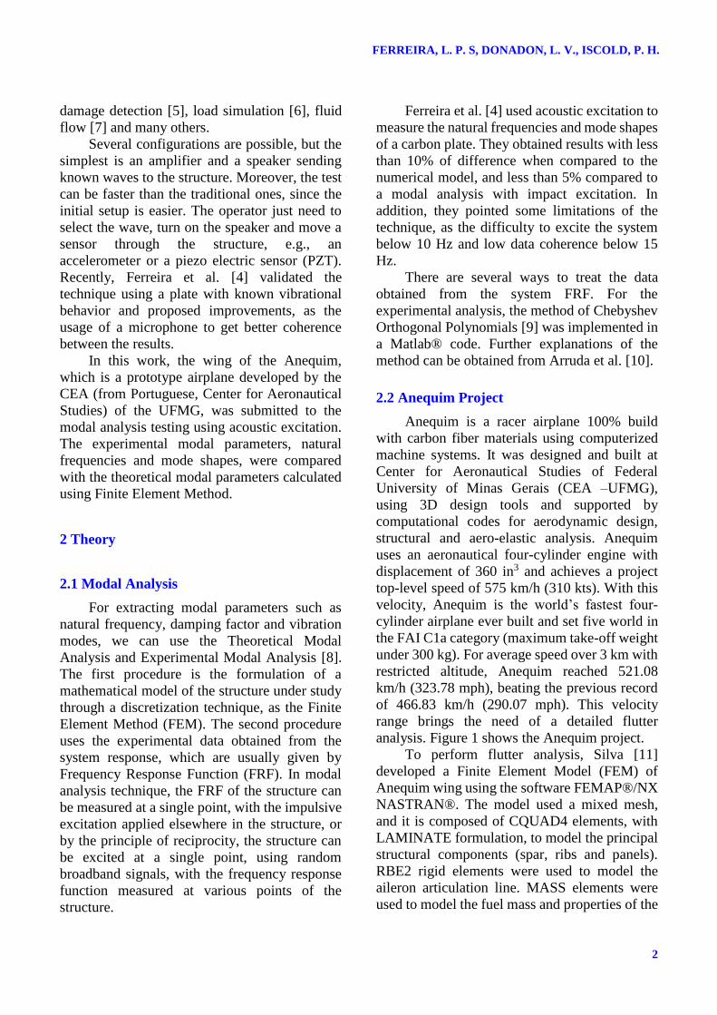
The wing was excited using a self-made 12

inches speaker and the response measured with a

PCB 333A3 accelerometer in each one of the 62

points (Fig. 4). The vibration data-

logger/analyzer used to record the signals was

LDS PHOTON II. The data were analyzed using

a Matlab® code with Chebycheff Orthogonal

Polynomials method to extract the experimental

natural frequencies and the mode shapes. The

LDS PHOTON II was used to generate the

excitation signal and send to the speaker. A PCB

microphone was placed between the speaker and

the wing to be used as the refence for the

Frequency Response Functions (FRFs). The

speaker was located under the wing around 200

mm. It is important to mention that the

experiments showed that the best excitation was

obtained with the speaker at the wing tip. The

experimental setup is shown in Fig. 5.

Fig. 4. Schematic diagram of the measurement points

0,00

0,15

0,30

0,45

0,60

0,75

0,90

-2,8 -2,4 -2,0 -1,6 -1,2 -0,8 -0,4 0,0

Ch

ord

Wingspan

5



According to Silva [11], the first five

fundamental frequencies occurs below 90 Hz.

Therefore, the excitation frequencies were

generated using a Sweep Sine with variable

amplitude and frequency from 5 Hz to 90 Hz in

three seconds. The measurements were

performed using a 240 Hz of sampling frequency

with 0.16 Hz of discretization frequency using

Hanning window. The system made 10

measurements and took the results average.

PHOTONCH1 CH2 CH3 CH4

SIGNAL

AC

CE

LE

RO

ME

TE

R

MIC

RO

PH

ON

E

WING

SPEAKER

SIGNAL GENERATOR

OR

Fig. 5. Acoustic excitation experimental assembly

4 Results and Discussions

4.1 Natural frequencies and modal shapes

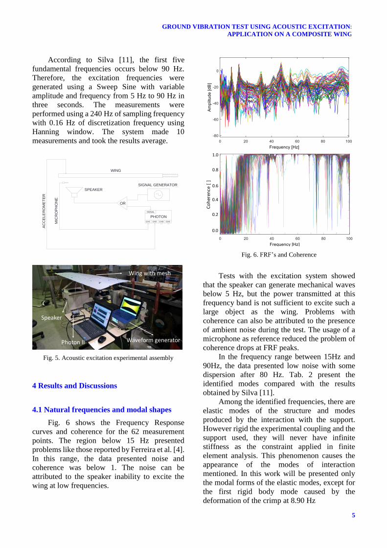
Fig. 6 shows the Frequency Response

curves and coherence for the 62 measurement

points. The region below 15 Hz presented

problems like those reported by Ferreira et al. [4].

In this range, the data presented noise and

coherence was below 1. The noise can be

attributed to the speaker inability to excite the

wing at low frequencies.

Fig. 6. FRF’s and Coherence

Tests with the excitation system showed

that the speaker can generate mechanical waves

below 5 Hz, but the power transmitted at this

frequency band is not sufficient to excite such a

large object as the wing. Problems with

coherence can also be attributed to the presence

of ambient noise during the test. The usage of a

microphone as reference reduced the problem of

coherence drops at FRF peaks.

In the frequency range between 15Hz and

90Hz, the data presented low noise with some

dispersion after 80 Hz. Tab. 2 present the

identified modes compared with the results

obtained by Silva [11].

Among the identified frequencies, there are

elastic modes of the structure and modes

produced by the interaction with the support.

However rigid the experimental coupling and the

support used, they will never have infinite

stiffness as the constraint applied in finite

element analysis. This phenomenon causes the

appearance of the modes of interaction

mentioned. In this work will be presented only

the modal forms of the elastic modes, except for

the first rigid body mode caused by the

deformation of the crimp at 8.90 Hz

Waveform generatorPhoton II

Speaker

Wing with mesh

0 10 20 30 40 50 60 70 80 90 1000

0.1

0.2

0.3

0.4

0.5

0.6

0.7

0.8

0.9

1

Frequency [Hz]

Co

he

ren

ce

[ ]

Co

her

ence

[ ]

1.0

0.8

0.6

0.4

0.2

0.0


6

Tab. 2. Comparison between experimental and numerical

frequencies from 15 Hz to 90 Hz

Mode

Numerical

Frequency

[Hz]

Experimental

Frequency

[Hz]

Mode

1 - 8.90 Rigid Body

2 19.6 14.7 First bendig

3 62.3 41.7 Second

Bending

4 69.7 49.4 Torsion

The natural frequencies obtained for all

modes were lower than the numerical ones. This

may be related to problems in the crimping, mass

differences between the model and the

simulation and differences in material properties.

Finite element models usually overestimate the

system stiffness. The adjustment of the numerical

model is beyond the scope of this work and will

be left as suggestions for future work. As an

example of a mode caused by the boundary

condition, Fig. 7 presents the mode of rotation

about the support.

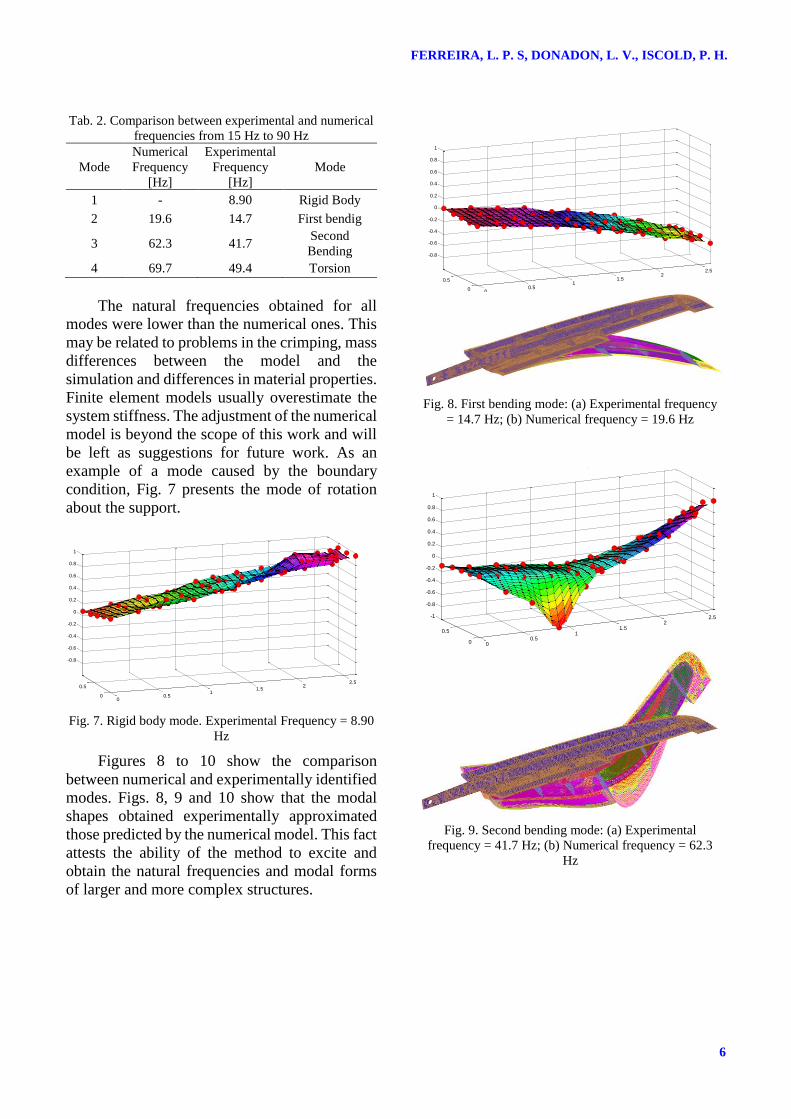
Fig. 7. Rigid body mode. Experimental Frequency = 8.90

Hz

Figures 8 to 10 show the comparison

between numerical and experimentally identified

modes. Figs. 8, 9 and 10 show that the modal

shapes obtained experimentally approximated

those predicted by the numerical model. This fact

attests the ability of the method to excite and

obtain the natural frequencies and modal forms

of larger and more complex structures.

Fig. 8. First bending mode: (a) Experimental frequency

= 14.7 Hz; (b) Numerical frequency = 19.6 Hz

Fig. 9. Second bending mode: (a) Experimental

frequency = 41.7 Hz; (b) Numerical frequency = 62.3

Hz

00.5

11.5

22.5

0

0.5

-0.8

-0.6

-0.4

-0.2

0

0.2

0.4

0.6

0.8

1

Mode Shape

00.5

11.5

22.5

0

0.5

-0.8

-0.6

-0.4

-0.2

0

0.2

0.4

0.6

0.8

1

Mode Shape

00.5

11.5

22.5

0

0.5

-1

-0.8

-0.6

-0.4

-0.2

0

0.2

0.4

0.6

0.8

1

Mode Shape

7



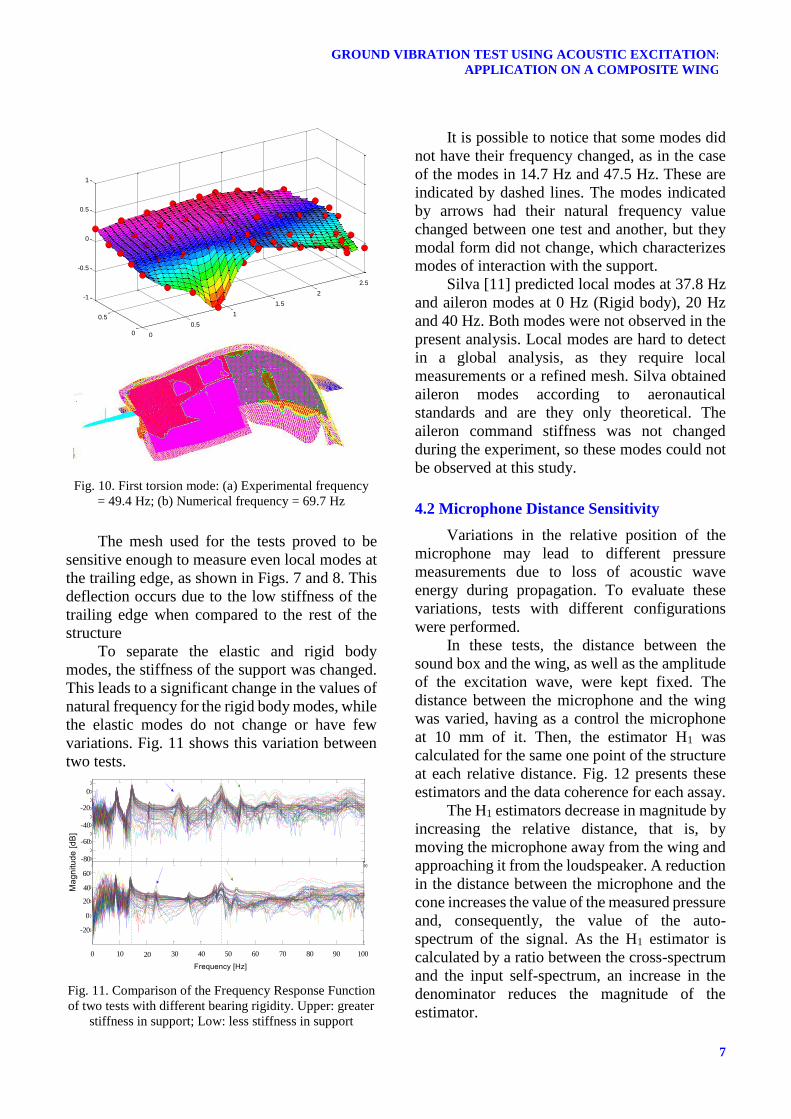
Fig. 10. First torsion mode: (a) Experimental frequency

= 49.4 Hz; (b) Numerical frequency = 69.7 Hz

The mesh used for the tests proved to be

sensitive enough to measure even local modes at

the trailing edge, as shown in Figs. 7 and 8. This

deflection occurs due to the low stiffness of the

trailing edge when compared to the rest of the

structure

To separate the elastic and rigid body

modes, the stiffness of the support was changed.

This leads to a significant change in the values of

natural frequency for the rigid body modes, while

the elastic modes do not change or have few

variations. Fig. 11 shows this variation between

two tests.

Fig. 11. Comparison of the Frequency Response Function

of two tests with different bearing rigidity. Upper: greater

stiffness in support; Low: less stiffness in support

It is possible to notice that some modes did

not have their frequency changed, as in the case

of the modes in 14.7 Hz and 47.5 Hz. These are

indicated by dashed lines. The modes indicated

by arrows had their natural frequency value

changed between one test and another, but they

modal form did not change, which characterizes

modes of interaction with the support.

Silva [11] predicted local modes at 37.8 Hz

and aileron modes at 0 Hz (Rigid body), 20 Hz

and 40 Hz. Both modes were not observed in the

present analysis. Local modes are hard to detect

in a global analysis, as they require local

measurements or a refined mesh. Silva obtained

aileron modes according to aeronautical

standards and are they only theoretical. The

aileron command stiffness was not changed

during the experiment, so these modes could not

be observed at this study.

4.2 Microphone Distance Sensitivity

Variations in the relative position of the

microphone may lead to different pressure

measurements due to loss of acoustic wave

energy during propagation. To evaluate these

variations, tests with different configurations

were performed.

In these tests, the distance between the

sound box and the wing, as well as the amplitude

of the excitation wave, were kept fixed. The

distance between the microphone and the wing

was varied, having as a control the microphone

at 10 mm of it. Then, the estimator H1 was

calculated for the same one point of the structure

at each relative distance. Fig. 12 presents these

estimators and the data coherence for each assay.

The H1 estimators decrease in magnitude by

increasing the relative distance, that is, by

moving the microphone away from the wing and

approaching it from the loudspeaker. A reduction

in the distance between the microphone and the

cone increases the value of the measured pressure

and, consequently, the value of the auto-

spectrum of the signal. As the H1 estimator is

calculated by a ratio between the cross-spectrum

and the input self-spectrum, an increase in the

denominator reduces the magnitude of the

estimator.

0

0.5

1

1.5

2

2.5

0

0.5

-1

-0.5

0

0.5

1

Mode Shape

0 10 20 30 40 50 60 70 80 90 100

-80

-70

-60

-50

-40

-30

-20

-10

0

10

Am

plitu

de

[d

B]

Frequência [Hz]

0 10 20 30 40 50 60 70 80 90 100

-20

0

20

40

60

Am

plitu

de

[d

B]

Frequência [Hz]100 20 30 40 50 60 70 80 90 100

-20

20

0

40

-80

60

-60

-40

-20

0


8

Fig. 12. FRF Estimator H1 (a) and coherence (b) for the

sensitivity test of the microphone position

The coherence of the data practically does

not change with the distance. This is because the

phase change between the wave picked up by the

microphone and the one that reaches the wing is

negligible. Considering excitations between 5 Hz

and 150 Hz, we have wavelengths of 68.0 m and

2.27 m, respectively. These wavelength values

are greater than the longer distance tested.

For the tests, a fixed distance equal to 10

mm between the wing and the microphone was

adopted to avoid compatibility problems between

FRF's.

4.3 External noise

As a method via acoustic excitation, the

result of the tests is influenced by ambient noise.

This occurs mainly in regions of low frequency

where the signal/noise ratio is lower. To

characterize the influence of noise on FRF,

measurements were taken at the CEA (Center for

Aeronautical Studies) where the tests were

performed both during the day, with people

working and machines in operation, and at dawn

when the ambient noise is lower. Fig. 12 shows

the frequency spectrum picked up by the

microphone for both conditions.

Fig. 13. Ambient noise where the tests were performed:

(a) at dawn and (b) during the day

One may notice an increase in peak

frequency in the spectrum captured during the

day. Spikes in a narrow frequency range are

assigned to structures or machines that generate

well-defined disturbances, such as motors or

pneumatic tools. In these, the frequency of

rotation or oscillation is practically constant,

which leads to narrow peaks in the spectrum. As

an example, the numerical cutting machine

present in the workshop operates at 8000 RPM or

133.3 Hz. This value can be observed in the

frequency spectrum as the last peak indicated to

the right.

In addition, an increase in the region

between 50 and 120 Hz can be observed, which

explains in part the noise observed in FRF's.

However, in this region the signal/noise ratio is

high, which reduces the influence of noise. The

evaluation of the influence of noise according to

the region can be done by observing Fig. 13. Here

we have the noise spectrum (a), two FRF's (b)

and the respective coherences (c). The functions

were chosen to portray the influence of noise on

points of different signal-to-noise ratios. Point 3

is located at the root of the wing, 400 mm from

the trailing edge. In addition, it is close to the

wing spar, which leads it to have few

displacements. Point 53 is located on the same

line along the chord, but at the tip of the wing,

which leads to large displacements, especially in

flexion or torsion modes.

(a)

(b)

9



Fig. 14. Evaluation of the influence of ambient noise: (a)

Noise spectrum, (b) FRF estimators and (c) Coherence

Observing Figs. 14 (b) and (c), although

both points have an abrupt coherence drop near

12 Hz, point 3 is more influenced by the presence

of low frequency noise. The decrease in 12 Hz is

caused by an increase in noise in this value, as

can be seen in Fig. 14 (a). However, after this

drop the coherence of point 53 returns to values

close to 1 and remains in this range, except for

some falls in peaks of antiresonance. Point 3 has

low coherence up to 20 Hz and still has a drop in

some noisy frequencies, such as 18 Hz, 38 Hz

and 75 Hz. This shows how much a low

displacement point is subject to noise

interference.

For this test, low-frequency vibrations are

the most difficult to treat because, in addition to

being inaudible, they are usually caused by large

structures that either are part of the environment

or are difficult to move. Vibrations of higher

frequencies, in addition to being audible, are

often attached to machines or people, which can

be turned off or minimized. Noise in an

experiment with acoustic excitation is difficult to

eliminate, especially when performed in an

environment such as a workshop or hangar.

However, the method proved to be robust enough

to identify vibration modes even with active

noises. In view of the application of the

technique, this robust character is essential, since

the movement of an aircraft or a large structure

to a different location for testing purposes is

impracticable. As a suggestion for noise

reduction, the test can be performed outside

working hours, such as night or dawn. This

would avoid displacement of the structure and

minimize noise caused by machines and

processes near the test site.

4.4 Evaluation of FRF estimators influence

According to Maia e Silva [12], the

estimators 𝐻1 , 𝐻2 and 𝐻3 are the most used in

the practical analysis. Also, the 𝐻3 estimator is

the one that suffers the least influence of external

noises.

The Photon II acquisition system allows

recording of data in time domain for the

subsequent treatment and calculation of the

desired estimator or the analysis in the frequency

domain with the real-time calculation of the 𝐻1

or 𝐻2estimators.

For the evaluation of the influence of the

estimators on the results, data were recorded in

time domain and the estimators were calculated

from it. In this comparison, an acquisition

frequency of 375 Hz was used and data were

recorded for 120 seconds at each measurement

point. For the frequency domain treatment, a

block size of 2000 points and the Hanning

window were used. Fig. 15 shows the mean of

the estimators in the frequency domain

calculated with the 62 measurements.

It can be noted that the three estimators

behaved similarly in the central region of the

frequency range, differing mainly in the

extremities. The 𝐻1 and 𝐻3 estimators present

less noise at low frequencies when compared

with the 𝐻2 estimator. In addition, they remain

very close throughout the frequency range,

except for the region below 5 Hz.

Fig. 15. Comparison between estimators H1, H2 e H3


10

5 Conclusion

The experiment showed that acoustic

excitation is a feasible technique in the studied

frequency range. This approach aims to facilitate

Groung Vibration Testing (GVT) and cause less

interference of electromechanical shakers in the

structure.

The technique was able to identify both the

overall modes of the structure and the rigid body

modes. Because it is a more complex structure, it

also has local modes that were identified mainly

in the trailing edge region, due to their lower

stiffness.

The influence of microphone distance,

ambient noise and different frequency response

function (FRF) estimators were also analyzed.

The results obtained attest to the ability of

the technique to excite and to identify modes of

vibrations of complex structures. They also prove

the robustness of the method to the influence of

external noise, since the tests were carried out in

a typical place of construction and storage of

aircraft. This is desirable because the movement

of an aircraft to a place of low ambient noise,

such as an anechoic chamber, is logistically

complicated.

However, more studies are needed to

determine the source of the problem with the

coherence below 15 Hz. As a suggestion for

future works would be to use a focused excitation

in this frequency with a bigger speaker or a

different type of signal. Another suggestion is to

measure the acceleration of both wings to

determine asymmetric and antisymmetric

configurations.

6 References

[1] Scanian, R.H., Rosenbaum, R. Aircraft vibration and

flutter; 1996.

[2] Allen, B., Harris, C., Lange, D., An inertially

referenced noncontact sensor for ground vibration

tests. Sound and Vibration, January 2010.

[3] Daborn, P.M., Ind, P.R., Ewins, D.J., Enhanced

ground-based vibration testing for aerodynamic

environments, Mechanical Systems and Signal

Processing, Volume 49, Issues 1–2, 20 December

2014, Pages 165-180.

[4] Ferreira, L. P. S., Donadon, L. V., Iscold, P. H,

Ribeiro, G. M., Modal analysis via acoustic

excitation – Application on a carbon plate. In

Proccedings of the International Symposium on

Solids Mechanics – MecSol 2015. Belo Horizonte,

Brasil

[5] Collini, L., Garziera, R., Mangiavacca, F.,

Development, experimental validation and tuning of

a contact-less technique for the health monitoring of

antique frescoes, NDT & E International, Volume 44,

Issue 2, March 2011, Pages 152-157.

[6] Assmus, M., Jack, S., Weiss, K.-A. and Koehl, M.

(2011), Measurement and simulation of vibrations of

PV-modules induced by dynamic mechanical loads.

Prog. Photovolt: Res. Appl., 19: 688–694.

[7] Zhang, M.M., Katz, J., Prosperetti, A., Enhancement

of channel wall vibration due to acoustic excitation of

an internal bubbly flow, Journal of Fluids and

Structures, Volume 26, Issue 6, August 2010, Pages

994-1017

[8] Souza, F.S., Análise modal em materiais compósitos

com adição de nanoparticulas. Term paper,

Universidade Federal de Minas Gerais, Belo

Horizonte, 2008

[9] Mason, J.C., Handscomb, D., Chebyshev

Polynomials. Chaoman & Hall/CRC, 2003

[10] Arruda, J. R. F. ; Rio, S. A. V. ; Santos, L. A. S. B. .

A space-frequency data compression method for

spatially dense laser Doppler vibrometer

measurements. Shock and Vibration, New York, NY,

v. 3, n. 2, p. 127-133, 1996.

[11] Silva, G. S, Análise De Flutter da Aeronave CEA 311

Anequim. Term paper, Universidade Federal de

Minas Gerais, Belo Horizonte, 2014

[12] Maia, N. M. M., Silva, J. M. M., Theoretical and

Experimental Modal Analysis, Hertfordshire,

Research Studies Press, 1997

7 Contact Author Email Address

mailto:[email protected]

Copyright Statement

The authors confirm that they, and/or their company or

organization, hold copyright on all of the original material

included in this paper. The authors also confirm that they

have obtained permission, from the copyright holder of any

third party material included in this paper, to publish it as

part of their paper. The authors confirm that they give

permission, or have obtained permission from the

copyright holder of this paper, for the publication and

distribution of this paper as part of the ICAS proceedings

or as individual off-prints from the proceedings.

Documents

GROUND VIBRATION TEST USING ACOUSTIC EXCITATION: … · 2018-10-27 · considering the tradeoff between refinement of the results and experimental time. The mesh consists of 62 points,